Finance and Economics Discussion SeriesDivisions of Research & Statistics and Monetary Affairs

Federal Reserve Board, Washington, D.C.

Machine Learning, the Treasury Yield Curve and RecessionForecasting

Michael Puglia and Adam Tucker

2020-038

Please cite this paper as:Puglia, Michael, and Adam Tucker (2020). “Machine Learning, the TreasuryYield Curve and Recession Forecasting,” Finance and Economics Discussion Se-ries 2020-038. Washington: Board of Governors of the Federal Reserve System,https://doi.org/10.17016/FEDS.2020.038.

NOTE: Staff working papers in the Finance and Economics Discussion Series (FEDS) are preliminarymaterials circulated to stimulate discussion and critical comment. The analysis and conclusions set forthare those of the authors and do not indicate concurrence by other members of the research staff or theBoard of Governors. References in publications to the Finance and Economics Discussion Series (other thanacknowledgement) should be cleared with the author(s) to protect the tentative character of these papers.

Machine Learning, the Treasury Yield Curve and Recession Forecasting

Michael Puglia Adam Tucker

michael.t.puglia@frb.gov adam.c.tucker@frb.gov

December 5, 2019

Abstract We use machine learning methods to examine the power of Treasury term spreads and other

financial market and macroeconomic variables to forecast US recessions, vis-à-vis probit regression. In particular we propose a novel strategy for conducting cross-validation on classifiers trained with macro/financial panel data of low frequency and compare the results to those obtained from standard k-folds cross-validation. Consistent with the existing literature we find that, in the time series setting, forecast accuracy estimates derived from k-folds are biased optimistically, and cross-validation strategies which eliminate data “peeking” produce lower, and perhaps more realistic, estimates of forecast accuracy. More strikingly, we also document rank reversal of probit, Random Forest, XGBoost, LightGBM, neural network and support-vector machine classifier forecast performance over the two cross-validation methodologies. That is, while a k-folds cross-validation indicates that the forecast accuracy of tree methods dominates that of neural networks, which in turn dominates that of probit regression, the more conservative cross-validation strategy we propose indicates the exact opposite, and that probit regression should be preferred over machine learning methods, at least in the context of the present problem. This latter result stands in contrast to a growing body of literature demonstrating that machine learning methods outperform many alternative classification algorithms and we discuss some possible reasons for our result. We also discuss techniques for conducting statistical inference on machine learning classifiers using Cochrane’s Q and McNemar’s tests; and use the SHapley Additive exPlanations (SHAP) framework to decompose US recession forecasts and analyze feature importance across business cycles.

Keywords: tree ensemble, Random Forest, XGBoost, LightGBM, neural network, support-vector machine, probit, recession, Treasury yield curve, Shapley

JEL Codes: C53, C45, E37

1

I. Introduction

It is well documented that an inverted Treasury yield curve is a strong signal of recession in the United States. In May 2018, the term spread between the 3-month Treasury bill discount and 10-year on-the-run yield-to-maturity – one of several common measures of the yield curve’s slope - narrowed to less than one percentage point for the first time since the Great Recession. The spread continued to decline and in May 2019 the yield curve inverted; that is to say, the 10-year yield-to-maturity fell below level of the 3-month bill discount. At time of writing (October 2019), the yield curve’s slope is 11 basis points.

The long-standing literature on forecasting recessions from financial market and macroeconomic data has used probit classification as its workhorse method. The predictive power of term spreads to forecast recession during the Volcker Era was particularly strong and the results of a probit regression of Treasury term spreads against an indicator of recession over a one- to four-quarter horizon will bear that out. Studies dating to the early 1990’s were first to make this case formally.

Virtually every study of this topic following those first published in the 1990’s has used some version of the probit method to investigate the problem, each extending the original studies in a new direction. Some researchers have sought out new data to augment the feature space, and credit or more broadly financial conditions appear to be an important input now, particularly during the Great Moderation. Other researchers, rather than seek out new features, have extended the probit method itself to test and control for a variety of the time-series properties of terms spreads and other inputs over recession.

In addressing the shortcomings of the standard probit method, all previous efforts essentially contend with one simple fact, which is that the probit framework is rigid. That rigidity can be credited to the probit link function. In order to classify data, the probit method attempts to draw a hyperplane through the feature space by minimizing a cost function. In doing so, the optimization must trade off goodness of fit in some areas of the feature space (by fitting the hyperplane separator well in those regions) against poorness of fit in other areas.

Machine learning methods - rooted in statistics and computer science - are an attractive alternative to the probit classification methods traditionally used in time-series macroeconometrics, particularly those that extend probit regression in complex ways (so as to address dynamic coefficient variation, structural breaks and serial correlation, etc.). Whereas probit methods must typically introduce additional parameters in order to create model flexibility, with machine learning flexibility is more often an innate feature of the methods, saving the researcher the task of reworking model specifications or the econometric approach when results are not satisfactory. That said, machine learning methods have the tendency to over-fit data, unless controlled sufficiently via a set of hyperparameters, which is not a problem that arises when probit methods are applied. Thus, the flexibility of machine learning methods also presents the researcher with new difficulties, which are managed via a bias-variance tradeoff.

In this paper we attempt a survey of machine learning methods and investigate their performance relative to probit methods in forecasting US recessions from financial market and macroeconomic data. Specifically we study artificial neural networks, support-vector machines and the

2

Random Forest, XGBoost and LightGBM algorithms (the latter three being presently some of the most popular tree ensemble methods in use). In service of this goal, we propose a novel strategy for conducting cross-validation on classifiers trained with macro/financial panel data of monthly frequency and compare the results to those obtained from standard k-folds cross-validation. We also discuss techniques for conducting statistical inference on machine learning classifiers using Cochrane’s Q and McNemar’s tests; and use the SHapley Additive exPlanations (SHAP) framework of Lundberg and Lee (2017) to decompose US recession forecasts and analyze feature importance across business cycles.

In a slight preview of our results we find that, consistent with established results, forecast accuracy estimates derived from k-folds cross-validation in time series settings are biased optimistically. Furthermore, we confirm that more conservative cross-validation strategies which eliminate data “peeking” produce lower, and perhaps more realistic, estimates of forecast accuracy. More strikingly, we also document rank reversal of probit, Random Forest, XGBoost, LightGBM, neural network and support-vector machine classifier performance over the two cross-validation methodologies we use. That is, while a k-folds cross-validation indicates that the forecast accuracy of tree methods dominates that of neural networks, which in turn dominates that of probit regression, the more conservative cross-validation strategy we propose indicates the exact opposite, and that probit regression should be preferred over machine learning methods, at least in the context of the present problem. This latter result stands in contrast to a growing body of literature demonstrating that machine learning methods outperform many alternative classification algorithms and we discuss some possible reasons for our result.

This paper is structured as follows. In the next section we survey the literature on forecasting recession from financial market data using probit methods, as well as the related machine learning literature. In Section III we describe the data used throughout the study. In Section IV we describe how the features in the data set are combined into a nest of models, to which classification algorithms (probit regression, neural networks, support-vector machines, Random Forest, XGBoost and LightGBM) are applied, and in Section V we describe the classification algorithms themselves. In Section VI we describe a novel cross-validation strategy for hyperparameter selection and forecast performance estimation, as well as our approach to classifier comparison and statistical inference. In Section VII we discuss the methods used to calculate feature importances. In Section VIII we present the results of cross-validation and compare classification methods. Those results are followed in Section IX by a discussion of the some of the salient features and economic implications of our findings, interpretation of the machine learning classifier outputs and forecast attribution using the SHAP framework. In Section X we conclude.

II. Review of the Literature

Prior to the 1990’s, econometric research examining the predictive power of financial variables was focused on forecasting macroeconomic outcomes such as real output and inflation. Much research since then – and that most relevant to the current paper - has examined the predictive power of financial variables to forecast future states of recession, rather than continuous measures of activity.

Estrella and Mishkin (1996, 1998) are early and oft-cited works that use financial and macroeconomic variables in a probit framework to forecast recession. They find that “stock prices are

3

useful with one- to three-quarter horizons, as are some well-known macroeconomic indicators,” for predicting recession. For longer horizons, however, they conclude that “the slope of the yield curve emerges as the clear individual choice and typically performs better by itself out-of-sample than in conjunction with other variables.” Indeed, for the recessions occurring during and before the Volcker Era, negative terms spreads turned out to be a very strong signal of impending recession.

The slope of the yield curve largely failed to predict the 1990-91 recession, however, or at least not as strongly as it had those before in the 1970’s and 1980’s. Dueker (1997, 2002) uses Markov switching in the probit framework to allow for coefficient variation and also investigates issues surrounding the application of probit methods to time-series data. He finds that, while it is important to allow for dynamic serial correlation of term spreads in the probit framework, “allowance for general coefficient variation is not particularly significant at horizons less than one year.”

Just prior to the onset of the 2001 recession, Chauvet and Potter (2001) extended the probit method to investigate the instability of the term spread’s predictive power and the possible existence of structural breaks. Using Bayesian techniques and several specifications of the probit method that variously allow for business-cycle dependence and autocorrelated errors, they find that “allowing for business-cycle-specific innovation variance and an autoregressive component has a much better in-sample fit than the original model of [Estrella and Mishkin].” They also find that recession forecasts from their more complicated extensions of the probit framework “are very different from the ones obtained from the standard probit specification.”

As the Great Recession loomed, and as the yield curve was beginning to invert again for first time since the 2001 recession, Wright (2006) re-examined the standard probit specification, looking more closely at the policy instruments and other financial variables of interest to the Federal Open Market Committee (FOMC). Including the level of the effective federal funds rate, the real federal funds rate (inflation) and a measure of term premiums in his analysis, he finds that adding the effective federal funds rate to a measure of the term spread improves predictive power and that “there is more information in the shape of the yield curve about the likely odds of recession than that provided by term spreads alone.” Around that same time, King, Levin and Perli (2007) embed credit spreads in the probit framework along with term spreads and find that predictive ability is improved, and type I error is reduced.1 They also incorporate Bayesian model averaging into the analysis, in another break with the standard probit framework, and find that “optimal (Bayesian) model combination strongly dominates simple averaging of model forecasts in predicting recessions.”

More recently, Fornani and Lemke (2010) extend the probit approach by endogenizing the dynamics of the regressors using a VAR and study the US, Germany and Japan. Liu and Moench (2016) use the receiver operating curve to assess predictive performance of a number of previously proposed variables. They find that, while “the Treasury term spread has the highest predictive power at horizons four to six quarters ahead, adding lagged observations of the term spread significantly improves the predictability of recessions at shorter horizons.” Favara, Gilchrist, Lewis and Zakrajsek (2016) decompose credit spreads and show that their power to predict recession is contained in a measure of investor risk appetite called the Excess Bond Premium (EBP), which is a feature used in this paper. Finally, Johansson and Meldrum (2018) use the principal components of the yield curve, as well as a measure of term

1 Unlike many of the previous studies, they limit their analysis to post-1987 data.

4

premiums to predict recession and Engstrom and Sharpe (2018) investigate the forecast power of near-term forward term spreads.

The methods used in the research described to this point (probit regression, Markov switching, Bayesian techniques, etc.) are well established in the field of econometrics. In contrast, the methods that we use in this paper have roots in statistics and computer science and - though used in industrial applications such as for credit scoring, actuarial modeling, online marketing, demand forecasting, etc. - have only in recent years found application in macroeconometric analysis. Fornaro (2016) uses large panels of predictors (several to hundreds) and adds to the probit framework a Bayesian methodology with a shrinkage prior for the parameters to predict recession. Ng (2014) dispenses with the probit framework altogether and applies a tree ensemble classifier2 to a panel of 132 real and financial features and their lags to do so. In contrast to Ng, in this paper we study a small panel of just 9 features and investigate the recession forecasting power of a broad cross-section of machine learning classifiers vis-à-vis probit methods. As previously mentioned, the methods we explore are artificial neural networks, support-vector machines, and the Random Forest, XGBoost and LightGBM algorithms. Finally, Holopainen and Sarlin (2017) use many of the machine learning methods used in this paper (and more) for the purpose of creating an early-warning/crisis detection mechanism for the Euro area. After conducting a horse race between the methods, their focus turns to model aggregation and ensemble voting techniques for producing forecasts from multiple classifiers. They also investigate the statistical significance of their results by means of bootstrap procedures.

In contrast to Holopainen and Sarlin’s work, in this paper we propose a very conservative nested time-series cross-validation procedure and explore strategies for contending with the time-series properties of macro panel data containing multiple structure breaks. Furthermore, we conduct statistical inference and classifier comparison by means of joint omnibus (Cochrane’s Q) and pairwise post hoc (McNemar’s) tests, rather than via bootstrap methods. We also apply the SHapley Additive exPlanations framework of Lundberg and Lee (2017) to investigate feature importance and decompose the forecasts of our classifiers.

The Random Forest method is a stable, well-studied tree-based ensemble algorithm used for both classification and regression. Its origins can be traced as far back as the 1960’s, when Morgan and Sonquist (1963) published the first paper on decision tree analysis, describing their AID (automatic interaction and detection) algorithm. In the early 1980’s, Breiman et al (1984) published the CART (Classification and Regression Trees) algorithm and reignited interest in decision trees. Decision tree classifiers suffer from several shortcomings however. Notably they are prone to over-fit and are sensitive to small perturbations in data, which render it difficult to balance bias and variance with them in supervised learning applications.

The Random Forest method proposed by Breiman (2001) corrects for these faults by introducing randomness into the decision tree algorithm and then aggregating the results of many decision trees. Each decision tree in a random forest is fit with a random subset of features from the pool of predictors and is trained on data sampled with replacement from the training set, a process known as bagging (bootstrap aggregating). Breiman shows that the Random Forest is robust to over-fitting and limits the bias traded against variance in supervised learning applications in ways that decision trees cannot.

2 Gradient boosting machines and the GBM package in R

5

The XGBoost (eXtreme Gradient Boosting) algorithm of Chen et al (2016) is a recent example of a general gradient boosting algorithm (to contrast with bagging algorithms like Random Forest). Gradient boosting methods were first proposed by Friedman (2001, 2002) and Mason et al (1999a, 1999b), and can also be used for both classification and regression. Tree-based boosting classifiers build decision trees sequentially, re-weighting misclassified instances on each iteration, and employ gradient descent to minimize a loss function. The AdaBoost algorithm of Freund and Schapire (1999) is an early example of a boosting algorithm that has found widespread use, but now it is but one of many and a growing number of such algorithms. XGBoost has been shown to possess a number of advantages over previous alternatives, notably speed and scalability.

Like XGBoost, LightGBM is a tree-based gradient boosting algorithm developed at Microsoft DMTK by Ke et al (2017) and open-sourced for public use. Though newer than XGBoost and not as widely used or tested, it has garnered interest in machine learning applications for its speed and, because its hyperparameter interface is very similar to XGBoost’s, ease of use.

Artificial neural networks trace their history the 1940’s. Early developments include Rosenblatt’s perceptron (1958), a simplified mathematical model of how biological neurons operate, which was subsequently implemented in computer hardware. Though developments towards today’s neural network architecture continued through the 1960’s, interest cooled considerably after Minsky and Papert (1969) proved the limits of the direction research on the topic had taken. During a relatively dormant period of work in the area, Werbos applied backpropagation (1974) to neural networks, which along with gradient descent forms the basis of modern-day training methods. Research interest gradually picked up again in the 1980’s with the advent of distributed, parallel computing, or connectionism as it was called at the time. Further development of the technology continued through the rest of the 20th century, but it has been the growing availability of commodity computing hardware over the past two decades that has made rapid advancement and widespread commercial application possible. Many open-source software packages for developing and training neural networks now exist, including scikit-learn, Tensorflow (Google) and PyTorch (Facebook) among others.

Support-vector machines were originally invented by Vapnik and Chervonenkis (1963) and grew in popularity after Boser, Guyon and Vapnik (1992) proposed the kernel trick for creating non-linear classifiers. Cortes and Vapnik (1995) introduced the soft margin classifier for handling noisy data. For a time these methods enjoyed a high degree of popularity among machine-learning practitioners, but more recently they have been surpassed in power by neural networks for many applications.

The empirical performance of machine learning methods on problems outside of the fields of finance and economics are well-documented. Fernandez-Delgado et al. (2014) studied 179 different binary classifiers on the 121 datasets in the UCI Machine Learning Data Repository.3 They found that, on average, Random Forest methods achieved the highest accuracy among all other families of classifiers, followed by support-vector machines and neural networks, and that in many cases the differences at the top of the list where not statistically significant. A similar study by Wainer (2016), using more robust hyperparameter searches, found Random Forest and gradient boosting to be two of the three top performing methods for classification, with the differences between the two methods also not

3 https://archive.ics.uci.edu/ml/index.php

6

statistically significant. Neither study utilized the (more recent) XGBoost or LightGBM packages specifically, but the former is currently the dominant statistical package in online data science competitions hosted by Kaggle4.

III. Data

The primary focus of this paper is to compare probit regression - used in most of the existing literature on forecasting recessions from financial market and macroeconomic data – to machine learning classifier algorithms. Our purpose is not to identify new features for forecasting recessions. As such, most of the features we have chosen for the analysis (6 of 9) are fairly standard in the literature and our results for models estimated via probit methods should be fairly well known. That said, we have experimented with two or three features that have not received much use in the published literature on this topic.

For a measure of terms spreads, or yield curve slope (Slope hereafter), we use the monthly average of the 10-year Treasury spot yield of Gurkaynak, Sack, and Wright (2006) less the monthly average of the 3-month Treasury bill discount in the Federal Reserve’s H.15 series. Consistent with Estrella and Mishkin (1998), we use the 3-month log difference of end-of-month S&P 500 index values (SP500 hereafter) to capture equity market developments. For a measure of credit market conditions, we use the Excess Bond Premium (EBP hereafter) of Gilchrist and Zakrajsek (2012), which is a monthly series. As in Wright (2006), the end-of-month values of the effective federal funds rate (FF) is used as the short-term rate of interest. In addition, we include the Federal Reserve Bank of Chicago’s National Financial Conditions Index (NFCI hereafter) as a measure of financial conditions more broad than that captured by the Excess bond premium and to our knowledge this is its first use in the literature.

In addition to these financial market inputs, we augment our feature space with two macroeconomic/business conditions indexes and a survey-based measure of recession probability. The 3-month log difference of the Conference Board’s Leading Economic Index (LEI hereafter), previously studied by Estrella and Mishkin (1998) and Dueker (1997) in the context of the present problem, is used in this study to capture macroeconomic conditions writ large. The highly correlated monthly average of the Aruoba-Diebold-Scotti business conditions index (ADS hereafter), which is comprised of several of the same macroeconomic data series5, is also used6. For our survey-based measure, we use the cumulative probability of recession over four quarters calculated from the Federal Reserve Bank of Philadelphia’s Survey of Professional Forecasters7 (SPF hereafter).

4 https://www.kaggle.com/ 5 Specifically, the index is comprised of (seasonally adjusted) weekly initial jobless claims, monthly payroll employment, industrial production, personal income less transfer payments, manufacturing trade and sales and quarterly real GDP. 6 Note that the ADS index - like the financial variables - is available in real-time, while the LEI and SPF are only available at a lag. This motivates our use of the ADS index, despite its high correlation (77%) with changes in the LEI. We must credit Viktors Stebunovs with introducing us to this feature and its use in the context of recession forecasting. 7 That is, the cumulated probability of recession assuming independence between quarters calculated from RECESS2 through RECESS5

7

Finally, we add a measure of term premiums to the analysis, with one small twist. While Wright (2006) and Johansson and Meldrum (2018) included measures of term premiums in their analysis (Cochrane and Piazzesi’s return forecasting factor and the 10-year term premium of Kim and Wright, respectively), here we use changes in term premiums, rather than levels. Specifically we use the 6-month percentage point change in the 5-year term premium of Adrian, Crump and Moench (ACM, 2013). We have chosen to use changes in term premiums (hereafter ACM5D) due to the well documented fact that the most widely used term structure “models produce different estimates for the levels of the term premia, but broadly agree on the trends and dynamics” (Cohen et al, 2018). We have chosen to use the ACM model specifically due to the widely held view that term premium estimates derived from the model are less persistent than alternative models (and so, in our view, perhaps more able to capture changes in the outlook for recession in a timely manner).

The recession indicator used in the analysis is the same as that used in most of the existing literature as well. For any given month, it is defined as true if any of the following twelve months falls within a recession, as defined by the National Bureau of Economic Research (NBER), and is false otherwise.8

All data is monthly, and covers the period from January 19729 to June 2019 (558 months or observations). Figure 1 below summarizes the nine data series. Shaded regions indicate recessions.

8 The Federal Reserve Bank of St. Louis, NBER based Recession Indicators for the United States from the Peak through the Trough [USRECM] series is used to define the latter occurrence. 9 January 1972 is the first month for which Excess Bond Premium is available.

8

Figure 1 - Summary of features. All series are monthly. 3m/10y Slope is the monthly average of the 10-year Treasury spot yield of Gurkaynak, Sack, and Wright (GSW) less the monthly average of the 3-month Treasury bill discount in the Federal Reserve’s H.15 series. Excess Bond Premium (EBP) is that of Gilchrist and Zakrajsek (2012). National Financial Conditions Index (NFCI) comes from the Federal Reserve Bank of Chicago. ADS Index is the monthly average of the Aruoba-Diebold-Scotti Business Conditions Index. LEI is the 3-month log-difference of the Conference Board’s Leading Economic Index. S&P500 is the 3-month log-difference of the equity index. The effective federal funds rate is month-end. SPF is the cumulative 4-quarter probability of recession calculated from the Federal Reserve Bank of Philadelphia’s Survey of Professional Forecasters RECESS series. ACM 5-year term premiums is a month-end value from the model of Adrian, Crump and Moench. The 6-month change in the ACM 5-year term premium of Adrian, Crump and Moench is a first difference in levels of average daily values. Shaded regions indicate recessions. Source: S&P 500 data from Bloomberg Finance LP, Bloomberg Per Security Data License.

The unconditional probability of the indicator across the entire dataset is 25.4% while the unconditional probability of recession in any given month over the entire dataset is 14.0%. The static moments, monthly volatility10, and the end-of-sample (June 2019) values of each series are summarized in Table 1.

Slope NFCI EBP S&P500 FF ADS LEI SPF ACM5D

Unconditional Mean 175 bps -0.02 6 bps 1.7% 5.17% -0.11 0.37% 53% -2 bps

Standard Deviation 140 bps 1.01 53 bps 7.3% 4.03% 0.89 1.86% 15% 47 bps

Monthly Volatility 40 bps 0.21 24 bps 5.1% 0.56% 0.39 0.71% 3.3% 29 bps

End-of-Sample Value (June 2019) -8 bps -0.78 -15 bps 3.0% 2.38% -0.15 0.00% 54% -24 bps

50% Prob. Level, Univariate Probit 34 bps 0.51 61 bps -11.3% 9.29% -0.81 -0.65% 65% 96 bps

Table 1 - Static Moments and Monthly Volatility of the Features

10 Monthly volatility is calculated assuming innovations are normally distributed.

9

In order to see more clearly the signal in the noise, Figure 2 shows the same data when each series is truncated at the level of 50% probability in a univariate probit regression against the recession indicator11, then rebased to zero. The last row of Table 1 lists the 50% probability level for each feature. Recessions prior the mid-1980’s were preceded by periods of strong inversion in term spreads and high short-term interest rates, while recessions after 1991 have been preceded by high levels of EBP (which is closely related to adverse credit conditions and/or credit investor risk aversion).12 The NFCI is partially correlated with the EBP, but fails to predict the recessions of 1991 and 2000. The ADS, LEI and SPF features appear to capture the 1991 recession more strongly than did the financial variables. Given the small, sparse nature of the data set, these facts likely explain most of its predictive power.

11 For the slope regression, this level is 34 basis points (i.e. yields curves flatter than 34 basis points signal greater than 50% probability of recession in the following 12 months.) For the EBP regression, this level is 61 basis points (i.e. EBP greater than 61 basis points signals greater than 50% probability of recession in the following 12 months). For the ADS regression, this level is -0.81 (i.e. an index level less than -0.81 signals greater than 50% probability of recession in the following 12 months). And so on… 12 Estrella and Mishkin (1996) noted that “restrictive monetary policy probably induced the 1973-75, 1980 and 1981-82 recessions but it played a much smaller role in the 1990-91 recession.” The latter could perhaps also be said of the 2001 recession and Great Recession as well.

10

Figure 2 – Recession signals in the data. All features are truncated at the level of 50% probability in a univariate probit regression against the occurrence of an NBER recession in the following 12 months, then rebased to zero. This is for expository and display purposes only; all analysis uses original data series. All series are monthly. Shaded regions indicate recessions.

11

IV. Models

Let us begin the present discussion by clarifying terminology. In machine learning studies generally, the concepts of a model, an algorithm and a classifier can be difficult to distinguish and the terms are often used interchangeably. Furthermore, there is a great deal of precedent in the fields of economics and finance that does not conform to conventions used in the disperse fields from which machine learning methods are derived. Here we use the following nomenclature:

• Model - A specification or collection of features (possibly transformed) representing the underlying economic system (e.g. a linear combination of variables, such as in the right hand side of a linear regression specification, or just a loose collection of features to be fed as one into a machine learning algorithm). Also called a hypothesis.

• Algorithm - A strategy or set of instructions for approximating a target function using a model

specification and data observations. In the present case, the target function is a recession forecast probability (or equivalently one that maps a recession label to a data point). Examples of classifier algorithms would include probit regression, neural networks or any other machine learning or econometric method. Also called a classifier algorithm or a learning algorithm. For practical purposes, algorithms exist as software packages to which researchers are able to apply models and data for the purpose of creating classifiers.

• Classifier - The result of applying a model and data to a classifier algorithm. A classifier is an

object that resides in computer memory after estimation is complete. In econometric terms, it is a sample from the space defined by a model and an algorithm over the data population. In order to compare the performance of two models or two algorithms, two classifiers must be estimated and the comparison must be made through the classifier samples. In contrast to the previous two concepts, which are abstract concepts for the present purposes, a classifier is a tangible machine that an econometrician can work on and study.

In this paper we study a large number of nested models, which is the subject of the present section. Denote the feature values in month t as 𝑆𝑆𝑆𝑆𝑆𝑆𝑆𝑆𝑆𝑆𝑡𝑡, 𝑁𝑁𝑁𝑁𝑁𝑁𝑁𝑁𝑡𝑡 , 𝐸𝐸𝐸𝐸𝐸𝐸𝑡𝑡, 𝑁𝑁𝑁𝑁𝑡𝑡, 𝑆𝑆𝐸𝐸500𝑡𝑡, 𝐴𝐴𝐴𝐴𝑆𝑆𝑡𝑡, 𝐿𝐿𝐸𝐸𝑁𝑁𝑡𝑡, 𝑆𝑆𝐸𝐸𝑁𝑁𝑡𝑡, 𝐴𝐴𝑁𝑁𝐴𝐴5𝐴𝐴𝑡𝑡. Furthermore, denote the response indicator, which takes a value of 1 if there is an NBER-dated recession in any of the twelve months following month t and is 0 otherwise, as 𝑁𝑁𝐸𝐸𝐸𝐸𝑁𝑁𝑡𝑡+1,𝑡𝑡+12. Finally, denote Φ() as the probit link function (the standard normal cumulative distribution), 𝑁𝑁𝑁𝑁() as neural network classifier algorithm over a collection of features, 𝑆𝑆𝑆𝑆𝐴𝐴() as a support-vector machine algorithm over a collection of features, 𝑁𝑁𝑁𝑁() as a Random Forest binary classifier algorithm over a collection of features, 𝑋𝑋𝑋𝑋𝐸𝐸() as an XGBoost binary classifier algorithm over a collection of features, and 𝐿𝐿𝑋𝑋𝐸𝐸() as a LightGBM binary classifier algorithm over a collection of features.

The first batch of nine models are univariate in each of the nine features. In the case of the Slope model, the probability of the indicator conditional on the model features for each classifier (i.e. the Slope classifiers to be estimated from the Slope model using the learning algorithms) is given by:

12

𝐸𝐸𝑃𝑃𝑃𝑃𝑃𝑃𝑃𝑃𝑃𝑃𝑃𝑃𝑡𝑡�𝑁𝑁𝐸𝐸𝐸𝐸𝑁𝑁𝑡𝑡+1,𝑡𝑡+12 = 1� = Φ(𝛼𝛼0 + 𝛼𝛼1𝑆𝑆𝑆𝑆𝑆𝑆𝑆𝑆𝑆𝑆𝑡𝑡)𝐸𝐸𝑃𝑃𝑁𝑁𝑁𝑁𝑁𝑁𝑃𝑃𝑁𝑁𝑁𝑁 𝑁𝑁𝑁𝑁𝑡𝑡𝑁𝑁𝑃𝑃𝑃𝑃𝑁𝑁�𝑁𝑁𝐸𝐸𝐸𝐸𝑁𝑁𝑡𝑡+1,𝑡𝑡+12 = 1� = 𝑁𝑁𝑁𝑁(𝑆𝑆𝑆𝑆𝑆𝑆𝑆𝑆𝑆𝑆𝑡𝑡)

𝐸𝐸𝑃𝑃𝑆𝑆𝑁𝑁𝑆𝑆𝑆𝑆𝑃𝑃𝑃𝑃𝑡𝑡−𝑉𝑉𝑁𝑁𝑉𝑉𝑡𝑡𝑃𝑃𝑃𝑃 𝑀𝑀𝑁𝑁𝑉𝑉ℎ𝑃𝑃𝑖𝑖𝑁𝑁�𝑁𝑁𝐸𝐸𝐸𝐸𝑁𝑁𝑡𝑡+1,𝑡𝑡+12 = 1� = 𝑆𝑆𝑆𝑆𝐴𝐴(𝑆𝑆𝑆𝑆𝑆𝑆𝑆𝑆𝑆𝑆𝑡𝑡)𝐸𝐸𝑃𝑃𝑅𝑅𝑁𝑁𝑖𝑖𝑅𝑅𝑃𝑃𝑅𝑅 𝐹𝐹𝑃𝑃𝑃𝑃𝑁𝑁𝐹𝐹𝑡𝑡�𝑁𝑁𝐸𝐸𝐸𝐸𝑁𝑁𝑡𝑡+1,𝑡𝑡+12 = 1� = 𝑁𝑁𝑁𝑁(𝑆𝑆𝑆𝑆𝑆𝑆𝑆𝑆𝑆𝑆𝑡𝑡)𝐸𝐸𝑃𝑃𝑋𝑋𝑋𝑋𝑋𝑋𝑃𝑃𝑃𝑃𝐹𝐹𝑡𝑡�𝑁𝑁𝐸𝐸𝐸𝐸𝑁𝑁𝑡𝑡+1,𝑡𝑡+12 = 1� = 𝑋𝑋𝑋𝑋𝐸𝐸(𝑆𝑆𝑆𝑆𝑆𝑆𝑆𝑆𝑆𝑆𝑡𝑡)𝐸𝐸𝑃𝑃𝑋𝑋𝑋𝑋𝑋𝑋𝑃𝑃𝑃𝑃𝐹𝐹𝑡𝑡�𝑁𝑁𝐸𝐸𝐸𝐸𝑁𝑁𝑡𝑡+1,𝑡𝑡+12 = 1� = 𝐿𝐿𝑋𝑋𝐸𝐸(𝑆𝑆𝑆𝑆𝑆𝑆𝑆𝑆𝑆𝑆𝑡𝑡) ⎭

⎪⎪⎬

⎪⎪⎫

(1)

Note that a constant is included when the probit method is used.

In the second batch of eight bivariate models, the Slope feature is combined with each of the other eight features. In the case of the Slope/LEI pair, the probability of the indicator conditional on the features for each classifier (i.e. the Slope/LEI classifiers to be estimated from the Slope/LEI model using the learning algorithms) is given by:

𝐸𝐸𝑃𝑃𝑃𝑃𝑃𝑃𝑃𝑃𝑃𝑃𝑃𝑃𝑡𝑡�𝑁𝑁𝐸𝐸𝐸𝐸𝑁𝑁𝑡𝑡+1,𝑡𝑡+12 = 1� = Φ(𝛼𝛼0 + 𝛼𝛼1𝑆𝑆𝑆𝑆𝑆𝑆𝑆𝑆𝑆𝑆𝑡𝑡 + 𝛼𝛼2𝐿𝐿𝐸𝐸𝑁𝑁𝑡𝑡)𝐸𝐸𝑃𝑃𝑁𝑁𝑁𝑁𝑁𝑁𝑃𝑃𝑁𝑁𝑁𝑁 𝑁𝑁𝑁𝑁𝑡𝑡𝑁𝑁𝑃𝑃𝑃𝑃𝑁𝑁�𝑁𝑁𝐸𝐸𝐸𝐸𝑁𝑁𝑡𝑡+1,𝑡𝑡+12 = 1� = 𝑁𝑁𝑁𝑁(𝑆𝑆𝑆𝑆𝑆𝑆𝑆𝑆𝑆𝑆𝑡𝑡 , 𝐿𝐿𝐸𝐸𝑁𝑁𝑡𝑡)

𝐸𝐸𝑃𝑃𝑆𝑆𝑁𝑁𝑆𝑆𝑆𝑆𝑃𝑃𝑃𝑃𝑡𝑡−𝑉𝑉𝑁𝑁𝑉𝑉𝑡𝑡𝑃𝑃𝑃𝑃 𝑀𝑀𝑁𝑁𝑉𝑉ℎ𝑃𝑃𝑖𝑖𝑁𝑁�𝑁𝑁𝐸𝐸𝐸𝐸𝑁𝑁𝑡𝑡+1,𝑡𝑡+12 = 1� = 𝑆𝑆𝑆𝑆𝐴𝐴(𝑆𝑆𝑆𝑆𝑆𝑆𝑆𝑆𝑆𝑆𝑡𝑡 , 𝐿𝐿𝐸𝐸𝑁𝑁𝑡𝑡)𝐸𝐸𝑃𝑃𝑅𝑅𝑁𝑁𝑖𝑖𝑅𝑅𝑃𝑃𝑅𝑅 𝐹𝐹𝑃𝑃𝑃𝑃𝑁𝑁𝐹𝐹𝑡𝑡�𝑁𝑁𝐸𝐸𝐸𝐸𝑁𝑁𝑡𝑡+1,𝑡𝑡+12 = 1� = 𝑁𝑁𝑁𝑁(𝑆𝑆𝑆𝑆𝑆𝑆𝑆𝑆𝑆𝑆𝑡𝑡 , 𝐿𝐿𝐸𝐸𝑁𝑁𝑡𝑡)𝐸𝐸𝑃𝑃𝑋𝑋𝑋𝑋𝑋𝑋𝑃𝑃𝑃𝑃𝐹𝐹𝑡𝑡�𝑁𝑁𝐸𝐸𝐸𝐸𝑁𝑁𝑡𝑡+1,𝑡𝑡+12 = 1� = 𝑋𝑋𝑋𝑋𝐸𝐸(𝑆𝑆𝑆𝑆𝑆𝑆𝑆𝑆𝑆𝑆𝑡𝑡 , 𝐿𝐿𝐸𝐸𝑁𝑁𝑡𝑡)𝐸𝐸𝑃𝑃𝑋𝑋𝑋𝑋𝑋𝑋𝑃𝑃𝑃𝑃𝐹𝐹𝑡𝑡�𝑁𝑁𝐸𝐸𝐸𝐸𝑁𝑁𝑡𝑡+1,𝑡𝑡+12 = 1� = 𝐿𝐿𝑋𝑋𝐸𝐸(𝑆𝑆𝑆𝑆𝑆𝑆𝑆𝑆𝑆𝑆𝑡𝑡 , 𝐿𝐿𝐸𝐸𝑁𝑁𝑡𝑡) ⎭

⎪⎪⎬

⎪⎪⎫

(2)

The third batch of tri-variate models combines Slope with two other variables that scored highly among the batch of 2-feature models. We continue in this fashion, forming batches of 4-, 5-, 6-, 7- and 8- feature models using the features appearing in the highest-performing models from the previous batch and combining with each of the remaining features. Due to computing constraints it is not feasible to estimate classifiers on models with all combinations of 1 to 9 features, so some subjective judgement is required between batches to identify those that are likely to perform well or otherwise be of interest to the analysis.

In total we compare 106 models, each estimated with all six algorithms using two cross-validation strategies, producing a total of 1272 classifiers. The models are listed in the Appendix in Table 13. Many of the models have been studied previously in the literature, particularly those that combine some of the Slope, LEI, EBP, SP500, FF and SPF features.

V. Algorithms

In this section, we provide a more detailed look at the machine learning methods studied in this

paper, and provide a more rigorous mathematical treatment of the training and prediction processes. Specifically, we cover the Random Forest, boosting (XGBoost and LightGBM), support-vector machine, and neural network algorithms. That said, we only seek to provide a greater intuition for these so-called “black box” methods, and encourage the interested reader to explore the cited papers more fully. In order to keep mathematical notation consistent, for the remainder of this section denote 𝑋𝑋 as the

13

design matrix of dimension 𝑛𝑛 × 𝑆𝑆 where each of the 𝑆𝑆 columns is a feature vector with 𝑛𝑛 observations. Similarly, define 𝑌𝑌 = (𝑦𝑦1,𝑦𝑦2, … , 𝑦𝑦𝑖𝑖) as the binary response vector. The classical binary response is typically coded as 𝑦𝑦𝑃𝑃 ∈ {0,1}; however, for the mathematical formulations of boosting and support vector machines, each 𝑦𝑦𝑃𝑃 ∈ {−1,1}. Finally, let 𝐿𝐿(𝑋𝑋′,𝑌𝑌′) be an arbitrary loss function with some inputs 𝑋𝑋′,𝑌𝑌′. Further notation will be introduced as needed.

As previously introduced, the Random Forest, formulated by Breiman (2001), is an ensemble of many decision trees, each trained over random bootstrap samples from the original data. Bootstrap resampling of training data is a process known as bagging (as in bootstrap aggregating) in the machine learning literature. In addition to bagging, the Random Forest method employs another process called feature bagging to further decorrelate the trees. Feature bagging is the selection of a random subset without replacement of features to be considered in the fitting process for each decision tree. That is, only bagged features are considered at each split in the tree. Training of the decision tree (i.e. determining the splits in the tree) is accomplished via the Classification and Regression Tree (CART) algorithm (Breiman et al 1984). Illustrating the algorithm is most easily done through the following pseudocode, where we define 𝑡𝑡(𝑋𝑋′,𝑌𝑌′) to represent a decision tree trained on some inputs 𝑋𝑋′,𝑌𝑌′ that optimizes some loss function 𝐿𝐿(𝑋𝑋′,𝑌𝑌′):

Algorithm 1: Random Forest For s =1 to S do

- Sample observations with replacement from 𝑋𝑋,𝑌𝑌 to create new training data, 𝑋𝑋𝐹𝐹,𝑌𝑌𝐹𝐹, of size 𝑛𝑛 (bagging) - Train a decision tree 𝑡𝑡𝐹𝐹(𝑋𝑋𝐹𝐹,𝑌𝑌𝐹𝐹), where each split in the tree considers 𝑘𝑘, 1 ≤ 𝑘𝑘 ≤ 𝑆𝑆, randomly sampled

without replacement feature vectors of 𝑋𝑋𝐹𝐹, optimizing 𝐿𝐿(𝑋𝑋𝐹𝐹,𝑌𝑌𝐹𝐹) (feature bagging)

End for

Classify new observations by taking the majority class vote of the 𝑆𝑆 trees trained, i.e. 𝑌𝑌� = 1 if 1𝑆𝑆∑ 𝑡𝑡𝐹𝐹(𝑋𝑋) ≥ 0.5𝑆𝑆𝐹𝐹=1

𝑆𝑆 and 𝑘𝑘 are taken to be free parameters in this algorithm and are tuned via cross-validation. There are additional regulation parameters 𝜔𝜔 that can be used to further tune the algorithm and control the bias-variance tradeoff (for instance, to control how deep a tree may be grown or how many nodes a tree may contain) but details on these other parameters are omitted for the sake of brevity13.

The loss function most commonly employed by the Random Forest and other methods using the CART algorithm is Gini impurity, which measures the chance of a randomly chosen element being misclassified, given the distributions of classes in the problem. Each split in the tree 𝑡𝑡𝐹𝐹(𝑋𝑋𝐹𝐹,𝑌𝑌𝐹𝐹) maximizes the amount of Gini impurity removed from the classification task over the 𝑘𝑘 variables considered. Other common choices of loss function are information gain, from information theory, for classification and variance reduction for regression.

Next, we present the general boosting framework first introduced by Friedman (2001, 2002) and Mason et al (1999a, 1999b) to describe the XGBoost and LightGBM methods. Boosting employs an iterative gradient descent algorithm to approximate a function, 𝐸𝐸(𝑋𝑋), that minimizes expected loss. This approximation to 𝐸𝐸(𝑋𝑋), denoted by 𝐸𝐸�(𝑋𝑋), is a weighted sum of many decision trees such that 𝐸𝐸�(𝑋𝑋) minimizes the empirical risk. In contrast to bagging in the Random Forest, the boosting method, at a

13 Some other parameters are explored in section VI. In addition, exploring package documentation, such as for the RandomForestClassifer class in the scikit-learn Python package, can be helpful.

14

general iteration step 𝑠𝑠, fits a new decision tree on the vector of “pseudo-residuals” in a greedy14 fashion rather than on the response 𝑌𝑌. More specifically, define the “pseudo-residuals” as:

𝜉𝜉𝐹𝐹� = − �𝛿𝛿𝐿𝐿�𝐸𝐸�(𝑋𝑋), 𝑌𝑌�

𝛿𝛿𝐸𝐸�(𝑋𝑋)�𝑋𝑋�(𝑋𝑋)=𝑋𝑋�𝑠𝑠−1(𝑋𝑋)

so that at step 𝑠𝑠, the boosting tree fits 𝑡𝑡𝐹𝐹(𝑋𝑋, 𝜉𝜉𝐹𝐹� ) rather than the bagged tree 𝑡𝑡𝐹𝐹(𝑋𝑋𝑆𝑆 ,𝑌𝑌𝐹𝐹) in the Random Forest algorithm. In other words, boosting methods train on the error of the previous iteration, so as to pass more weight on to misclassified examples and less to correctly classified examples. Again, using pseudocode to describe this procedure from Friedman (2001):

Algorithm 2: General boosting framework Create a base classifier to initialize the fitting process 𝐸𝐸�0(𝑋𝑋) = 𝑎𝑎𝑃𝑃𝑎𝑎𝑎𝑎𝑎𝑎𝑛𝑛𝜋𝜋𝐿𝐿(𝜋𝜋,𝑌𝑌) For s =1 to S do

Compute “pseudo-residuals” 𝜉𝜉𝐹𝐹� = −�𝛿𝛿𝛿𝛿(𝑋𝑋�(𝑋𝑋),𝑌𝑌)𝛿𝛿𝑋𝑋�(𝑋𝑋) �

𝑋𝑋�(𝑋𝑋)=𝑋𝑋�𝑠𝑠−1(𝑋𝑋)

Fit 𝑡𝑡𝐹𝐹�𝑋𝑋, 𝜉𝜉𝐹𝐹� � Find optimal 𝜋𝜋𝐹𝐹 by solving 𝑎𝑎𝑃𝑃𝑎𝑎𝑎𝑎𝑎𝑎𝑛𝑛𝜋𝜋𝐿𝐿�𝐸𝐸�(𝑋𝑋)𝐹𝐹−1 + 𝜋𝜋𝑡𝑡𝐹𝐹�𝑋𝑋, 𝜉𝜉𝐹𝐹� �,𝑌𝑌� Set 𝐸𝐸𝐹𝐹�(𝑋𝑋) = 𝐸𝐸�𝐹𝐹−1(𝑋𝑋) + 𝜋𝜋𝐹𝐹𝑡𝑡𝐹𝐹(𝑋𝑋, 𝜉𝜉𝐹𝐹� ) End for Classify new observations using 𝐸𝐸𝑆𝑆�(𝑋𝑋)

𝑆𝑆 is taken to be a free parameter in this algorithm to be tuned during cross-validation. In most implementations there will exist other free parameters 𝜔𝜔 can be used to further tune the algorithm (for instance, to control the depth of trees or the maximum number of nodes in any tree). Similarly to Random Forests, boosting is adaptive to a variety of loss functions. The choice of function depends on the problem at hand - classification or regression - and on the utility of the econometrician. In this study, we utilize binary logistic loss for boosting methods.

The Random Forest and boosting methods share the free parameters 𝑆𝑆 and 𝜔𝜔, which control the number of trees grown in the algorithms, as well as the depth and number of nodes in any particular tree. Each individual tree grown can be described as a weak learner in that the generalization of any tree is often poor. However, combining many of these weak learners in an ensemble is what drives the predictive power of the methods. Our choice of 𝜔𝜔 is the solution to a bias-variance tradeoff problem in classical statistics, with the added wrinkle that we must also consider computational feasibility when working with most boosting algorithms. A small 𝜔𝜔 may increase computational efficiency and bias, while keeping prediction variance low. Conversely, a large 𝜔𝜔 may increase the variance and computational load, but reduces bias. The following section presents more information on the various parameters encountered in the algorithms and our cross-validation strategy for tuning them.

Moving on we present the support-vector machine method originally proposed by Vapnik and Chervonenkis (1963). A support-vector machine classifier attempts to construct a pair of parallel hyperplanes to separate data with the largest possible margin between classes. For illustrative purposes, we consider a linear support-vector machine in 2-dimensions with data that is perfectly separable (or hard-margin, to contrast with soft-margin). In this simple case, there are many lines that

14 Greedy in this context refers to an algorithm that makes a locally optimal decision at each iteration with the intent to converge on a global optimum.

15

define a margin separating the classes in the data; however the support-vector machine finds those which maximize the distance to the nearest data point in each class. Consider two parallel lines defined by:

𝑤𝑤��⃗ ∙ �⃗�𝑥 − 𝑏𝑏 = ±1

As shown in the figure below by the two dashed black lines, if the parameters of the lines are chosen appropriately, a margin between the classes in the data is formed. The distance between these lines is given by:

2‖𝑤𝑤��⃗ ‖

To maximize the distance between the lines, minimize ‖𝑤𝑤��⃗ ‖ subject to the constraint 𝑦𝑦𝑃𝑃(𝑤𝑤��⃗ ∙ �⃗�𝑥 − 𝑏𝑏) ≥ 1 (i.e. so that no data points fall inside the margin). The solution to this problem defines the classifier �⃗�𝑥 →sgn(𝑤𝑤��⃗ ∙ �⃗�𝑥 − 𝑏𝑏).

Figure 3 - Illustration of a support-vector machine. This is a simple depiction of a (hard-margin) linear support-vector machine in two dimensions. The data points are color-coded by class. The sample on the margins of the dashed black lines are support vectors and the region between the lines is the maximum margin. The red line in the center of the margin is the maximum-margin hyperplane.

In this simple case, the support-vector machine is not that different from a probit regression, but the support-vector machine can be modified to be more flexible. For example, for data that is not separable, the hinge loss function can be introduced (soft-margin). For non-linear boundaries, kernel functions can be introduced. In our application, we search over 2nd, 3rd, and 4th order polynomial kernel functions during cross-validation.

To conclude this section, we turn to the artificial neural network classifier. Artificial neural networks approximate non-linear regression and classification functions through a collection of nodes organized into multiple layers. The figure below depicts a simple example of a neural network classifier with three input vectors, two hidden layers with four nodes each and a single output node.

16

Figure 4 - Illustration of a feed-forward neural network. This is a simple feed-forward neural network shown for illustrative purposes. It contains two hidden layers, with four nodes each. Data from the leftmost layer, the input layer, is passed into the hidden layers, which transform the data. Values from the hidden layers are passed to the rightmost layer, the output layer, which is an indicator of class probability in classification problems. Bias (constant) nodes may also be employed, but are omitted in the figure.

The first layer, the input layer, passes the data vectors 𝑥𝑥1, 𝑥𝑥2, 𝑥𝑥3 into hidden layer 1. Each node 𝑦𝑦𝑃𝑃 in hidden layer 1 uses a weighting vector 𝑎𝑎𝑃𝑃 (displayed as edges or arrows into the node) to linearly transform the information from the input layer, 𝑎𝑎𝑃𝑃0 + 𝑎𝑎𝑃𝑃1𝑥𝑥1 + 𝑎𝑎𝑃𝑃2𝑥𝑥2 + 𝑎𝑎𝑃𝑃3𝑥𝑥3, and then employs a (possibly) non-linear activation function f to construct the layer outputs at each node:

𝑦𝑦𝑃𝑃 = 𝑓𝑓(𝑎𝑎𝑃𝑃0 + 𝑎𝑎𝑃𝑃1𝑥𝑥1 + 𝑎𝑎𝑃𝑃2𝑥𝑥2 + 𝑎𝑎𝑃𝑃3𝑥𝑥3)

Common choices of the activation function include the hyperbolic tangent function and the logistic function amongst others. In this study the rectified linear unit (ReLU) is used. This procedure continues to the right for each node in each hidden layer. The last layer of the neural network, the output layer, transforms the values from the final hidden layer into the output values of the network, which in the binary classification setting is a single node denoting the indicator class probability.

Like the neural network depicted above, in this study we use a relatively simple architecture, consisting of just two hidden layers. We make no attempt to cross-validate over the number of nodes in each layer (or over more exotic architectures such as recurrent or convolution networks or those employing other features such as dropout). The number of nodes used in each layer is a stepwise function of the number of features in the model being trained, as follows (neglecting the bias nodes):

17

# of Model Features, k # Nodes, Hidden Layer 1 # Nodes, Hidden Layer 2 0<k≤3 9 5 3<k≤6 12 6

k≥7 18 9 Table 2 - Neural Network Architectures. The neural network architectures used in this study, as a function of model features is shown above. Bias nodes are not included in the counts.

Neural networks are trained on data (i.e. the weights are chosen) using backpropagation and gradient descent. Backpropagation is an iterative method that exploits the chain rule to update node weights in a neural networks so as to minimize a loss function. In this study cross-entropy loss is targeted.

VI. Classifiers and Cross-Validation

In this section we outline our approach to 1) selecting hyperparameters for the algorithms, 2) estimating the out-of-sample forecast performance of each classifier and 3) comparing classifiers across models and algorithms. Ultimately our goal is to determine what, if any, value the machine learning methods add to our ability to forecast recession vis-à-vis the probit method. The data set presents several challenges that motivate our overall strategy for doing so. Those challenges can be summarized as follows:

- The data set is serially correlated, which violates the i.i.d. assumption required to use many of the cross-validation methods most popular in the machine learning literature, such as k-folds, leave-p-out, etc. Furthermore, because the data is time-series and not cross-sectional in nature, attempting k-folds cross validation on the data set would result in “data peeking” and overly optimistic estimations of forecast performance.

- The data set likely contains one if not multiple structural breaks (delineated by the Volcker Fed, the Great Moderation and the Financial Crisis perhaps), further violating the i.i.d. assumption and also making standard time-series cross-validation methods such as sliding or expanding windows problematic.

- The indicator (recession) is unbalanced in the data set (unconditional mean of ~25%) and occurs temporally in clusters of varying length at the end of each business cycle, further complicating the use of standard time-series cross-validation methods such as sliding or expanding windows.

- The data set is relatively short (558 observations) and sparse over the joint feature space.

Our strategy for contending with these features of the data is to implement a 4-fold nested time-series (NTS) cross-validation to estimate out-of-sample forecast performance for each combination of the 106 models and 6 algorithms under study. Originally designed by Varma and Simon (2006) for use on small datasets to address the unique difficulties they pose, according to Raschka (2018) nested cross-validation “shows a low bias in practice where reserving data for independent test sets is not feasible.” We augment the standard nested cross-validation strategy to incorporate several features that make it more amenable to conducting time-series analysis on the small macro/financial panel dataset under study in this paper, and to address the serial correlation, indicator imbalance and structural breaks that

18

are present (hence the name nested time-series cross-validation). In particular, we overlay standard nested cross validation with an expanding window, so as to respect the time ordering of the data and prevent future leakage. We add one wrinkle to this feature in that, rather than forward chaining the window over a single data point or a fixed-size block of data points, we forward chain the outer loop of the NTS cross validation over business cycles.

The NTS cross-validation procedure we use is most easily described by means of the following pseudo-code algorithm:

Algorithm 3: Nested Time-Series (NTS) Cross-Validation Algorithm Function: nested_time_series_cv(model, algo, data, grid, metric) Input: model (specification of features used to forecast recession), algo (classification algorithm, such as probit, neural network, random forest, etc.), data (dataset of feature and indicator observations stratified into k = 7 folds by business cycle), grid (discrete set in algo’s hyperparameter space to be searched for optimal performance), metric (forecast performance metric function and basis for model/algo comparison, e.g. accuracy, AUCROC) Output: performance (forecast performance estimate for model/algo combination, in units of metric) OUTER LOOP (expanding window cross-validation) For i = 3 to k-1 do Hold out data fold i+1 for use as an outer loop test set. Use data folds 1 to i as an outer loop training set. Stratify the outer loop training set by fold, shuffle over the stratified classes and divide into 3 folds of equal size. HYPERPARAMETER GRID SEARCH Foreach j ∈ grid do INNER LOOP (standard 3-fold stratified/shuffled cross-validation) For m = 1 to 3 do Hold out fold m from the outer loop training set as an inner loop test set. Use the folds {n:n∈{1,2,3},∼(n∈{m})} of the outer loop training set as an inner loop training set. Estimate a classifier for model using algo, the inner loop train set and hyperparameters j. inner score[m] ← calculate forecast performance for inner loop m using metric and the inner loop test set. End for hyperparameter score[j] ← average of inner score[1:3] for hyperparameters j. End foreach optimal hyperparameters[i] ← element in grid with the highest hyperparameter score Estimate a classifier for model using algo, the outer loop train set and optimal hyperparameters[i] outer score[i] ← calculate forecast performance for outer loop i using metric and the outer loop test set. End for performance ← average of outer scores[3:k]. Return performance

To be more concrete, consider the top panel of Figure 5, where we plot real GDP growth over our sample period, indicating recession periods in gray above the x-axis. Colored regions below the x-axis demarcate the individual business cycles that comprise the data; each colored region begins in a period of economic growth and ends when the NBER recession period following the period of growth terminates.

19

Figure 5 - Data Folds Used in Time-Series Nested Cross Validation Procedure. In the top panel, Real GDP growth is plotted over the sample period. Gray shaded regions above the x-axis indicate recession periods. Colored regions below the x-axis demarcate the business cycles that comprise the data set. In the lower panel, the correspondence between the business cycles and the data folds used in cross-validation is shown.

The bottom panel of Figure 5 shows each iteration of the NTS cross-validation outer loop in a row. Within each iteration of the outer loop, a stratified/shuffled 3-fold cross-validation is conducted over each training set (labeled Train) to determine optimal hyperparameters. The optimal hyperparameters are then used to estimate a classifier over the full training set, and the outer loop iteration is scored by calculating forecast performance (e.g. accuracy) over the test set (labeled Test) using the estimated classifier. When all 4 iterations of the outer loop are complete, the model/algorithm pair is scored by the average out-of-sample forecast performance over the 4 iterations.

The first three business cycles are used for training in the first iteration of the outer loop due to their relatively short durations, and to ensure a large enough sample for classifier estimation. It is our opinion that the division of the data and the NTS cross-validation strategy described above represents the best balance that can be achieved between 1) size of the training/test sets on one hand, 2) sample size of the outer loop forecast accuracy estimate and 3) indicator imbalance in the data.

Two main alternatives to this cross-validation strategies exist, but when applied to time series data they become problematic, in that they do not always respect the time ordering of data. The first alternative is a standard k-folds cross-validation strategy, originally developed for use on cross-sectional

20

data that obeys an i.i.d. assumption. It is widely recognized that this strategy is not appropriate for time series data and results is overly optimistic estimates of forecast performance. The second alternative is a hybrid approach, somewhat between a standard k-folds cross-validation strategy and the NTS cross-validation strategy described above. While it is generally accepted that the time-ordering of data must be respected when estimating classifier forecast performance, it is less clear whether it is necessary to respect the time-ordering of data when determining the optimal hyperparameters of the classifier algorithm. A strategy in which optimal hyperparameters are chosen through a strategy such as k-folds cross-validation on the entire data set, but then forecast performance is estimated using a rolling or expanding window strategy and the optimal hyperparameters determined by k-folds, would respect the time-ordering of data during the latter half of the exercise, but violate it during the former. Holopainen and Sarlin (2016) implement a hybrid strategy similar to this and find ultimately that “conventional statistical approaches are outperformed by more advanced machine learning methods.” In this paper we’ve taken a more conservative approach in using the NTS cross validation strategy, precluding any violation of the time-ordering of data during the study. In a later section we will discuss the possible implications of our choice, and we present results from NTS cross-validation and k-folds cross-validation side-by-side for comparison.

With regards to the forecast performance metric, we use accuracy as the target value over which hyperparameters are selected and out-of-sample forecast performance is measured. Our choice of forecast accuracy as a scoring metric within the NTS cross validation procedure is motivated by several considerations. Though we would have preferred to use average precision (AP) of the precision-recall curve to score forecast performance, the last business cycle in the sample does not yet contain a positive instance of the indicator (recession),15 and so AP is ill-conditioned in that business cycle during NTS cross-validation. We also considered area under the receiver operating curve (ROCAUC). Like AP, however, ROCAUC is also ill-conditioned when a positive instance of the indicator does not exist and in any case Davis and Goadrich (2006) show that, in this setting, the area under the receiver operating characteristic curve does not give a complete picture of a classification method’s performance16. Since accuracy and Brier score are well-behaved over the last business cycle, they remain as the best candidates for scoring forecast performance. For the present analysis we have chosen to use accuracy as the target metric.

The grid search that is used in the inner loop of the NTS cross-validation procedure is the principle means by which variance is traded against bias for the machine learning algorithms. For example, if the tree-based methods (Random Forest, XGBoost, LightGBM) are allowed to grow too deeply, or if neural networks with a large number of neurons and hidden layers are used, the methods are prone to overfit data, resulting in high forecast variance, which is perhaps the main difficulty that arises in working with the algorithms.

For each of the tree-based algorithms, we search over a subset of about five of the hyperparameters exposed. Since each of the algorithms has a different set of hyperparameters it is

15 The current business cycle began in 2009 and continues to present without recession, representing the longest uninterrupted economic expansion in U.S. history. As such the latter 10 years of data, or about 21% of the sample, contains no positive instances of a recession indicator. 16 Furthermore they show that any method that dominates in the precision-recall space also dominates in the receiver operating characteristic space.

21

difficult to draw direct comparisons between them, but generally there are a few main parameters used in each to control overfitting and balance speed of estimation against accuracy. The ensemble methods’ hyperparameter “number of iterations” or “number of trees” dictates the number of weak learners created. Setting this number too low can cause models to not capture the signal in the data, but setting this number too high will almost certainly result in an infeasible computation time. For the Random Forest and XGBoost algorithms, the “maximum depth” hyperparameter (exposed in all of the major implementations of these algorithms) is a strong control. LightGBM also has a maximum depth hyperparameter, but a separate parameter controlling the maximum number of leaves in an individual tree is more readily able to control overfitting. For the 1-feature models, maximum depth is limited to be at most 3 in the grid search; for the 2-feature models it is limited to 4; while for all other models it is limited to 5. While this restriction may seem arbitrary, we found its interpretation and symmetry to be pleasing.17 As a practical matter, we also found the restriction to be very necessary in light of our very small and sparse dataset.

Where the neural network and the support-vector machines are concerned, the situation is greatly simplified. We were able to obtain satisfactory results using neural networks with a simple two hidden-layer architecture of roughly 12 and 6 neurons respectively (slightly less for the models with just a couple features, and slightly more for models with seven or eight, as shown in Table 2). We made no attempt to optimize over the neural network architecture, though it is possible our results could be improved by doing so. For support-vector machines, the kernel function search was limited to 2nd, 3rd and 4th order polynomials. Finally, note that, since the probit method does not have hyperparameters, grid-search cross-validation is not necessary and the inner loop can be forgone, which renders our strategy equivalent to time-series expanding windows (over business cycles) cross-validation in this special case.

After applying the NTS cross-validation strategy to our models, algorithms and data, we will be left with 636 estimates of forecast performance across all combinations of 106 models and 6 algorithms, from which we hope to choose those that work best for the problem at hand. Accounting for estimation uncertainty is critical to this exercise. Unfortunately this is a topic of research that is still developing in the machine learning literature and there does not yet exist a generally accepted approach to statistical inference or classifier comparison. In this paper we rely heavily on the strategies suggested in Raschka (2018).

The first stage of our model comparison amounts to what is effectively an omnibus F-test over our classifiers. Rather than group all of our classifiers into a single test, however, we group them once by model and again by algorithm, to identify the dimensions along which large, statistically significant differences in forecast performance may exist, and those along which they do not. More specifically, we use Cochran’s Q Test, which tests the null hypothesis that there is no difference between the grouped classifier forecast accuracy estimates. Consider the group of six classifiers for a single model x (the 1-feature Slope model, for instance). The null hypothesis 𝐻𝐻0 is:

𝐻𝐻0:𝐴𝐴𝑥𝑥,Φ = 𝐴𝐴𝑥𝑥,𝑁𝑁𝑁𝑁 = 𝐴𝐴𝑥𝑥,𝑆𝑆𝑉𝑉𝑀𝑀 = 𝐴𝐴𝑥𝑥,𝑅𝑅𝐹𝐹 = 𝐴𝐴𝑥𝑥,𝑋𝑋𝑋𝑋𝑋𝑋 = 𝐴𝐴𝑥𝑥,𝛿𝛿𝑋𝑋𝑋𝑋

17 That is, for the Random Forest and XGBoost algorithms, a 1-feature model could have up to 8 leaves (23), a 2-feature model up to 16 (24) and a 3-feature model up to 32 (25). The breakdown for LightGBM is slightly more complicated.

22

where 𝐴𝐴𝑥𝑥,𝑦𝑦 is the forecast accuracy of the classifier estimated on model x, algorithm y. If the 𝑎𝑎 = 6 classifiers for the model do not differ in forecast performance, then Cochran’s Q statistic for model x, defined below, will be distributed approximately χ2 with 𝑎𝑎 − 1 degrees of freedom:

𝑄𝑄𝑥𝑥 = (𝑎𝑎 − 1)𝑎𝑎∑ 𝑋𝑋𝑃𝑃2 − 𝑇𝑇𝑥𝑥2𝑅𝑅

𝑃𝑃=1

𝑎𝑎𝑇𝑇 − ∑ 𝑎𝑎𝑗𝑗2𝑖𝑖

𝑗𝑗=1

where 𝑛𝑛 = 558 is the total number of observations in the data set; 𝑎𝑎𝑗𝑗 is the number of classifiers out of m that correctly classified the jth observation in the data set; 𝑐𝑐𝑥𝑥,𝑦𝑦,𝑗𝑗 is 1 if the classifier for model x, algorithm y correctly identified the jth observation and 0 otherwise; and:

𝑋𝑋𝑃𝑃 = ∑ 𝑎𝑎𝑗𝑗𝑖𝑖𝑗𝑗=1 𝑇𝑇𝑥𝑥 = ∑ ∑ 𝑐𝑐𝑥𝑥,𝑃𝑃,𝑗𝑗

𝑖𝑖𝑗𝑗=1

𝑅𝑅𝑃𝑃=1

Similarly we could group the classifiers by algorithm (neural networks for instance) and conduct the omnibus test in that dimension. In this case the null hypothesis 𝐻𝐻0 is:

𝐻𝐻0:𝐴𝐴𝑥𝑥1,𝑁𝑁𝑁𝑁 = 𝐴𝐴𝑥𝑥2,𝑁𝑁𝑁𝑁 = ⋯ = 𝐴𝐴𝑥𝑥𝑘𝑘,𝑁𝑁𝑁𝑁

where again 𝐴𝐴𝑥𝑥,𝑦𝑦 is the forecast accuracy of the classifier estimated on model x, algorithm y. If the 𝑎𝑎 =106 classifiers for the algorithm do not differ in forecast performance, then Cochran’s Q statistic for algorithm y, defined below, will be distributed approximately χ2 with 𝑎𝑎 − 1 degrees of freedom:

𝑄𝑄𝑦𝑦 = (𝑎𝑎 − 1)𝑎𝑎∑ 𝑋𝑋𝑃𝑃2 − 𝑇𝑇𝑦𝑦2𝑅𝑅

𝑃𝑃=1

𝑎𝑎𝑇𝑇 − ∑ 𝑎𝑎𝑗𝑗2𝑖𝑖

𝑗𝑗=1

where

𝑇𝑇 = ��𝑐𝑐𝑃𝑃,𝑦𝑦,𝑗𝑗

𝑖𝑖

𝑗𝑗=1

𝑧𝑧

𝑃𝑃=1

and all other quantities are the same as for 𝑄𝑄𝑥𝑥.

Note that in the case of 𝑄𝑄𝑥𝑥, the grouping of classifiers by sixes keeps the individual tests reasonably small. In effect, the hypothesis that 𝑄𝑄𝑥𝑥 tests is along the lines of “does it matter which algorithm is used to estimate this model?” If the null hypothesis is rejected, it suggests that at least one classifier is greatly outperforming or underperforming the others, and that further investigation is warranted. In the case of 𝑄𝑄𝑦𝑦, however, grouping 106 classifiers at a time is fairly pointless. In a sample so large it is almost certain that one classifier will perform differently than the rest. In order to address this issue (that is, to pose a more reasonable hypothesis) some a priori means of first filtering among the 106 models is required before applying Cochran’s Q test along that dimension. In a later section we will discuss the means by which we select down from 106 to just 8 classifiers before applying the test.

If the null hypothesis is rejected during one of the omnibus tests, we have reason to conclude that a statistically significant difference in forecast performance exists among the classifiers. In the second stage of our model comparison, we conduct pairwise post-hoc tests, with adjustments for multiple comparisons, to determine where the differences occur. In particular, we use pairwise McNemar (1947) or Chi-square within-subjects tests between all classifiers in the grouping. To do so, we first construct 2x2 contingency tables for each pairing of classifiers in the group, shown below:

23

c2 correct c2 incorrect c1 correct A B

c1 incorrect C D

In the contingency table, A is the number of observations out of n=558 that both classifier 1 and 2 classified correctly. B is the number of observations that classifier 1 classified correctly and classifier 2 identified incorrectly, and vice-versa for C. D is the number of observations that both classified incorrectly. Note that 𝐴𝐴 + 𝐸𝐸 + 𝑁𝑁 + 𝐴𝐴 = 𝑛𝑛 and that the accuracy of classifier 1 and 2 is:

𝐴𝐴𝑐𝑐𝑐𝑐𝐴𝐴𝑃𝑃𝑎𝑎𝑐𝑐𝑦𝑦1 = 𝐴𝐴+𝑋𝑋𝑖𝑖

𝐴𝐴𝑐𝑐𝑐𝑐𝐴𝐴𝑃𝑃𝑎𝑎𝑐𝑐𝑦𝑦2 = 𝐴𝐴+𝐶𝐶𝑖𝑖

Note also that the differences between the classifiers are captured by B and C, so these are the natural quantities of interest to the problem at hand. If the null hypothesis is that the probabilities of B and C are equal (i.e. both classifiers have the same rate of error), then McNemar’s statistic, defined below, will be distributed χ2 with one degree of freedom.

McNemar′s χ2 =(𝐸𝐸 − 𝑁𝑁)2

𝐸𝐸 + 𝑁𝑁

Edwards (1948) proposed a continuity correction to this statistic, which becomes:

McNemar′s χ2 =(|𝐸𝐸 − 𝑁𝑁| − 1)2

𝐸𝐸 + 𝑁𝑁

If the null hypothesis is rejected after application of McNemar’s test to a pairing of classifiers, we may conclude that the classifier with the higher forecast accuracy estimate outperforms the other and that the difference is statistically significant.

VII. Feature Importances

After the forecast performances of all models and algorithms have been determined in NTS cross validation and weighed against one another by means of the omnibus Cochran’s Q and pairwise McNemar tests presented in the previous sections, it is natural to ask which of the nine features under study contributed to the overall performance of the classifier and how. In this section we outline a few methods for doing so.

At this point of the analysis we dispense with NTS cross-validation and calculate our feature importance metrics in-sample. That is, we use the entire data set as a training sample, use k-folds cross-validation to determine optimal hyperparameters, then estimate classifiers using the optimal hyperparameters, and then calculate feature importances by means of the estimated classifiers. It is not clear whether this is a valid approach. We know that the (out-of-sample) forecasts from NTS cross-validation differ greatly from in-sample forecasts, and forecasts estimates are an important input to some of the metrics we use (e.g. SHAP values) as will be shown below. We also know that it is

24

preferable to calculate some importance metrics (e.g. permutation importance or mean decrease in accuracy) out-of-sample, but it is generally common practice to calculate them in-sample. Our reason for calculating feature importance in-sample is mainly practical. First, it would require a great deal of new machinery to integrate the metrics into the NTS cross-validation strategy we propose. Second, even if that were theoretically possible (which is not yet clear) we would have serious issues of computational feasibility to contend with. As such, we move forward using in-sample metrics from this point and leave those considerations to future work.

The feature importance metrics that we consider fall into two broad categories: those that are specific to only one or a few algorithms and those that can be applied broadly to all algorithms. In the probit literature referenced in Section II, it is common practice to report the sensitivity or marginal effects of an estimated model as a measure of variable importance. This is an example of the former type of feature importance, since it relies on the parametric nature of the probit method and cannot be applied directly to the machine learning methods we study. The sensitivity metric has many variations, but in essence all of them are partial derivatives of the output probability with respect to the inputs at some point in the feature space. One commonly used variation of the metric calculates these partial derivatives at each point in the dataset used for estimation and averages over all observations. That is, the sensitivity of the probit classifier to the kth feature fk is:

𝑆𝑆𝑆𝑆𝑛𝑛𝑠𝑠𝑎𝑎𝑡𝑡𝑎𝑎𝑖𝑖𝑎𝑎𝑡𝑡𝑦𝑦𝑓𝑓𝑘𝑘 =1𝑛𝑛�

𝜕𝜕Φ�𝛼𝛼0 + ∑ 𝛼𝛼𝑗𝑗𝑓𝑓𝑗𝑗𝑅𝑅𝑗𝑗=1 �

𝜕𝜕𝑓𝑓𝑁𝑁�𝑓𝑓1..𝑚𝑚=𝑂𝑂𝑃𝑃𝐹𝐹𝑖𝑖

𝑖𝑖

𝑃𝑃=1

where k=1…m; m is the total number of features in the model; αk, k=1…m are the estimated coefficients; Obsi is the set of feature values in observation i=1…n; and n is the total number of observations. Other variations may use the partial derivative evaluated at some other point in the feature space, such as the unconditional mean of the features.

A more useful importance metric for the present study is the permutation importance, or mean decrease in accuracy (MDA) metric. Originally proposed by Breiman (2001), the calculation of this metric uses bootstrap methods, allowing it to be applied broadly to any classifier. The algorithm is most easily described via the pseudo-code below:

Algorithm 4: Permutation Importance (Mean Decrease in Accuracy) Algorithm Function: permutation_importance(classifier, data, n_iter, frac) Input: classifier (an estimated classifier on a model/algo pair, data (dataset of n observations of m features and indicator), n_iter (number of iterations) frac (fraction of data observations sampled without replacement on each iteration) Output: mda (vector permutation importances or mean decrease in accuracy for each feature) For i = 1 to n_iter do Randomly sample frac% of observations from data to create a bootstrap set data_i acc_base_i←calculate accuracy of classifier on data_i For j = 1 to m do Permute column j in data_i to create bootstrap/permuted set data_i_j acc_ij←calculate accuracy of classifier on data_i_j da[i][j]←acc_base_i – acc_ij End for End for mda[j=1..m]← average of da[j=1..m] over all n_iter iterations Return mda

25

For each iteration in the outer loop of the algorithm, a fraction of the observations (perhaps 70%) are sampled from the data to create a bootstrap sample. Baseline accuracy for the sample set is then calculated and recorded, before entering the inner loop of the algorithm. On each iteration of the inner loop, a single feature’s column is permuted to break the association between the feature and indicator in the data. Accuracy of the classifier on the bootstrap/permuted data set is then calculated, and the decrease in accuracy from the baseline level that results is recorded. When all iterations (perhaps 10 or 100, depending on sample size) of the outer loop are complete, the sampled decreases in accuracy for each feature are averaged over the number of outer loop iterations to produce the mean decreases in accuracy for each feature. Features with large MDA’s indicate that classifier accuracy will suffer if removed from the model and re-estimated, and those with low MDA’s indicate that classifier accuracy will not change greatly if removed.

An argument can be made that a classifier’s MDA should not be calculated on the same data used to train the classifier, but rather a test or validation set that is held out. Due to the many data issues described already, and because we will have documented forecast performance prior to calculating these feature importance metrics, we calculate MDA on our entire data sample. While this may be cause for criticism, most of the recession forecasting literature uses in-sample data when calculating probit classifier sensitivities as well. We also feel that, while absolute forecast performance estimates will likely be overstated if the time ordering of the data is not respected during cross validation (necessitating the proper use of test sets and cross-validation methods that preclude data peeking) it is not clear that relative feature importances (which are probably more germane to this discussion than absolute feature importances) will be so greatly impacted if calculated using in-sample data.

Data issues aside, the feature importance metrics described so far - probit sensitivities and permutation importances – belong to a class of so-called global feature attribution methods, in that they score the value of a feature to a classifier as a whole through a single summary metric. No further decomposition of individual predictions is possible under this class of methods.

If feature attribution at the level of a single observation is desired, a local method is required. The SHapley Additive exPlanations (SHAP) framework of Lundberg and Lee (2017) provides an example. While other local feature attribution methods exist, such as LIME (Reibero et al, 2016) and DeepLIFT (Shrikumar et al, 2017), Lundberg and Lee demonstrate that SHAP unifies these approaches and others under a more general framework for decomposing individual predictions and attributing feature importance.

At the core of the SHAP framework, the Shapley value is a concept from coalitional game theory that prescribes how gains or “payouts” resulting from a cooperative game should be divided amongst players in proportion to their contribution to the outcome. In the present case, the players are the features in the dataset and the “payout” is the forecast probability output by the classifier given the observations at time t18. More technically, consider the set f of m features in the dataset at time t, and a classifier prediction function v that maps the feature values at t to a probability forecast 𝑖𝑖(𝑓𝑓) ∶ 2𝑅𝑅 →

18 The payout can also be interpreted as the forecast probability of the classifier in excess of the naïve or (unconditional) mean forecast probability of the classifier over all observations.

26

Ρ . If s is a coalition or subset of features 𝑠𝑠⊂𝑓𝑓, then v(s) describes the worth of coalition s, or the total “payout” (i.e. probability) that the members of s can expect to receive by working together.

The Shapley value suggests a way to distribute the total forecast probability to the grand coalition of all features f after considering all possible coalitions and their individual worths. The Shapley value, which in the present case is the amount of “probability” apportioned to feature i in f at t, is given by:

𝜑𝜑𝑃𝑃(𝑖𝑖) = �|𝑠𝑠|! (𝑎𝑎 − |𝑠𝑠| − 1)!

𝑎𝑎!𝐹𝐹⊆𝑓𝑓\{𝑃𝑃}�𝑖𝑖(𝑠𝑠 ∪ 𝑎𝑎) − 𝑖𝑖(𝑠𝑠)�

The second term inside the summation can be interpreted as the amount of payout fairly credited to feature i if i were to join coalition s. The summation is conducted over all subsets s of f not containing feature i, or rather all permutations of coalitions s that i does not belong to but could join. In effect, feature i’s total payout is the average of its payouts over all those permutations.

The Shapley value is considered to be a fair attribution of the total probability in the sense that it possesses a few desirable properties. Those pertinent to the present discussion are summarized as follows:

• Efficiency - The Shapley values for all features in the set f add up to the total payout v. That is ∑ 𝜑𝜑𝑃𝑃(𝑣𝑣)

𝑅𝑅𝑃𝑃=1 = 𝑖𝑖(𝑓𝑓). In other words, the Shapley values for the features f at time t

sum up to the probability forecast of the classifier given the observation at time t.

• Symmetry - If two features contribute equally to all permutations of coalitions, then their Shapley values are equal. That is, if features i and j satisfy 𝑖𝑖(𝑠𝑠 ∪ {𝑎𝑎}) = 𝑖𝑖(𝑠𝑠 ∪ {𝑗𝑗}) for every coalition 𝑠𝑠⊆𝑓𝑓\{𝑎𝑎, 𝑗𝑗} then 𝜑𝜑𝑃𝑃(𝑖𝑖) = 𝜑𝜑𝑗𝑗(𝑖𝑖).

• Null Player - If a feature cannot contribute to any coalition to which it is not a member, than its Shapley value is zero. That is, if 𝑖𝑖(𝑠𝑠 ∪ {𝑎𝑎}) = 𝑖𝑖(𝑠𝑠) for every coalition 𝑠𝑠⊆𝑓𝑓\{𝑎𝑎} then 𝜑𝜑𝑃𝑃(𝑖𝑖) = 0.

Though these ideas form the basis of the SHAP framework, direct implementation of Shapley values in a machine learning setting is generally not feasible, since it may require the classifier to be retrained on all the permutations of 𝑠𝑠⊆𝑓𝑓\{𝑎𝑎} for each feature i in the data set (as well as all observations t). In order to apply Shapley values in practice, an approximation is required. The SHAP framework unifies several local Shapley value approximation methods under a more general conditional expectation function of an abstract machine learning model. In general, each of these local approximation methods maps to a single class of machine learning algorithms. The SHAP methods relevant to the present discussion and the algorithms they map to are:

• TreeSHAP –SHAP value approximation for tree ensembles (Lundberg et al, 2018). We apply TreeSHAP to the Random Forest, XGBoost and LightGBM classifiers in this study.

• DeepSHAP – SHAP value approximations for deep neural networks. This method wraps DeepLIFT (Shrikumar et al, 2017). Though we study neural network classifiers in this paper,

27

the DeepSHAP framework will not integrate with our implementation19, and so we use the more generally applicable KernelSHAP for neural network SHAP value decomposition.

• KernelSHAP – SHAP value approximations for general functions. This method uses LIME (Reibero et al, 2016) to locally approximate any classifier function. We apply KernelSHAP to the probit, support-vector machine and neural network classifiers in this paper (i.e. all except the tree ensembles).

VIII. Results

We begin by presenting the results of NTS cross-validation across all models and all algorithms. As mentioned in the previous section, we have chosen accuracy to score the models. Table 14 in the appendix shows accuracy estimates for each model and classifier with standard errors, as well as the mean accuracies conditional on the model. Rows are sorted in order of decreasing mean accuracy conditional the model. The top 5 individual classifiers are highlighted in dark orange. The “best-in-class” nest of models (to be defined shortly) is highlighted in light orange.

Much of the information in Table 14 can be summarized and more easily ascertained in Figure 6 below, which scatterplots the estimates of classifier forecast accuracy against the number of features in its model. The points are color-coded by algorithm. The dashed lines connect the means of the forecast accuracy estimates conditional on algorithm and number of features.

19 DeepSHAP integrates with neural networks built in Tensorflow/Keras and PyTorch but not scikit-learn. We have used scikit-learn.

28

Figure 6 - Nested Time-Series Cross-Validation Results. Mean out-of-sample forecast accuracy for each model and classifier, estimated using nested time-series cross-validation, is scattered against the number of features in its model above. Points are color-coded by algorithm. The dashed lines connect the means of estimated forecast accuracies conditional on algorithm and number of features and are color-coded consistent with the scatter points. Data can be found in Table 14.

The first column of Table 3 below repeats the bottom row of Table 14, which is the mean forecast accuracy, conditional on algorithm, across all 106 models, with conditional standard errors in parenthesis. The second column weights the conditional mean and standard errors calculation (Cochran 1977) to control for the varying sample size within each tier of models with the same number of features (because some algorithms perform better with a few number of features, and others may perform better on many features). The results are generally consistent between the two methods of calculation. As a first order consideration, probit performs the best, followed generally by neural networks and/or LightGBM, then XGBoost, Random Forest and/or support-vector machines.

Algorithm Mean Forecast Accuracy (SE)

Averaged over Models Averaged over Models and # Features Probit 0.878 (0.0046) 0.868 (0.0176)

NN 0.867 (0.0054) 0.858 (0.0171) LightGBM 0.865 (0.0052) 0.861 (0.0181) XGBoost 0.863 (0.0061) 0.853 (0.0176)

RF 0.854 (0.0065) 0.841 (0.0168) SVM 0.854 (0.0075) 0.842 (0.0157)

Table 3 – Nested Time-Series CV Mean Forecast Accuracy, Conditional on Algorithm. Mean out-of-sample forecast accuracy across all models, conditional on algorithm, using nested time-series cross-validation is reported in the table above. Standard errors of the mean accuracy estimate are in parenthesis.

29

Table 16 in the Appendix reports the means of the estimated forecast accuracies, conditional on algorithm and number of features. They are plotted below as well (and in Figure 6 as dotted lines).

Figure 7 - Nested Time-Series Cross-Validation Conditional Mean of Estimated Forecast Accuracy. Means of estimated forecast accuracy conditional on algorithm and number of features, as well as means of the estimated forecast accuracy conditional on the model and number of features. Select models are label with their name. Data can be found in Table 16.

A few features stand out in the figures above and their table equivalents in the appendix:

1) Before considering the statistical significance of the results, the probit methods seem to outperform the other algorithms generally across all models, at least up through 6 features. Neural networks appear to be a close second over many models, though LightGBM is sometimes competitive. XGBoost, Random Forest and support-vector machines generally round out the bottom of the ranking, in that order.

2) The best single model generally was the 7-feature Slope/LEI/ACM5D/NFCI/EBP/SPF/SP500

model. This model also nests many of best-performing 2-, 3-, 4-, 5- and 6-feature models as well, as highlighted in light orange in Table 14. The best single classifier was the 6-feature Slope/ADS/NFCI/EBP/ACM5D/SPF probit classifier, highlighted in dark orange in Table 14. Two of the top five classifiers were probit classifiers and two were neural networks.

30

3) Among the 1-feature models, the forecast performance of LEI, NFCI, SPF and ADS exceeded that of Slope, in that order. Slope outperformed EBP, SP500, ACM5D and FF, which is consistent with the literature.

4) The 2-Feature Slope/LEI model is ranked 12th in Table 14, and the 3-feature Slope/LEI/ACM5D is ranked 7th, both higher than many models with far more features. This highlights the high degree of forecast power that Slope and LEI contain.

5) The worst performing models generally include the effective federal funds rate.20 Even when combined with other features that together perform well, the federal funds rate appears to diminish the power of a model, particularly if estimated by probit regression.

6) Accuracy increases generally in the number of features used, up to 7 features, then declines. It seems that 4 features is better than 1, but it is not clear that 7 is necessarily better than 4, after taking into account classifier variance. This topic will be addressed in more detail shortly.

Next we compare the results of NTS cross-validation to 5-fold cross validation. Stratification is used when forming folds, due to the class imbalance in the indicator series and to ensure that the training and testing sets contain similar proportions of positive and negative instances. Furthermore, shuffling is employed to contend with the existence of structural breaks in the data.21 Table 15 in the appendix shows the results of 5-fold cross-validation for each model and classifier, as well as the averages conditional on the model. Rows are sorted in order of decreasing mean accuracy conditional the model. The top 5 individual classifiers are highlighted in dark orange. The “best-in-class” nest of models from NTS cross-validation (which again will be defined shortly) is highlighted in light orange, for comparison.

For the purposes of comparing the two cross-validation strategies, we have included one 12-feature and one 20-feature model, in addition to those described in Section IV. The 12-feature model begins with the nine features under study and adds the natural rate of interest (r-star) of Laubach and Williams (2003), GARCH(1,1) conditional volatility of West Texas Intermediate (WTI) spot crude oil prices and GARCH(1,1) conditional volatility of the Federal Reserve’s Trade Weighted U.S. Dollar Index. All three of these features have very low recession forecasting power and essentially amount to noise in the algorithms. The 20-feature model further adds 1) the near-term forward term spread of Engstrom and Sharpe (2018), the 6-month percentage point change in the 10-year term premium as well as the levels of the 5-year and 10-year term premiums of Adrian, Crump and Moench (ACM, 2013), the Treasury 3-month bill discount, the real Federal Funds rate (as defined in Wright, 2006) and the default and “GZ” spread of Gilchrist and Zakrajsek (2012), all of which also either amount to noise in the algorithms or are highly correlated with some of the nine features under study. Our purpose for doing this is mainly to investigate the robustness of both the algorithms and the cross-validation methodologies to noisy or redundant (co-linear) features.

20 Though Wright (2006) found this feature to have predictive power, that study was conducted prior to recent experience with the effective lower bound. 21 In particular, the StratifiedKFold cross-validator in the scikit-learn package is used, with shuffling enabled.

31

The results are displayed in Figure 8 below in two panels. The panel on the left shows the results from NTS cross validation, and like Figure 6 it scatterplots the estimates of classifier forecast accuracy against the number of features in each model, color-coding points by algorithm and showing the means of the forecast accuracy estimates conditional on algorithm and number of features as dashed lines. The panel on the right shows the results from 5-fold cross-validation in the same format.

Figure 8 – Comparison of Nested Time-Series and k-Folds Cross-Validation Results. The panel on the left displays the results of nested time-series cross-validation, while the panel on the right shows the same information for 5-fold cross-validation. Both panels display the number of features on the x-axis, and the estimates of mean forecast accuracy on the y-axis. Both panels are scatterplots of the estimates of classifier forecast accuracy against the number of features in each model estimated, and are color-coded by algorithm. The dashed lines are the means of the forecast accuracy estimates conditional on algorithm and number of features. Data can be found in Table 14 and Table 15.

A few conclusions may be drawn from the figure:

- The accuracy estimates from k-folds cross-validation are higher than the estimates from NTS cross-validation. This seems to hold no matter the criteria used to make this assessment. The highs are higher, the lows are higher, and the means and medians are higher all along the curves shown. This is consistent with the existing literature and here we have it is very clear visual form.

- The accuracy estimates from NTS cross-validation, conditional on algorithm and number of features have much higher variance than k-folds cross-validation. This calls into question whether the k-folds cross-validated classifiers, which have been allowed to “peek” at future data before forecasting a sample that is held out, are truly able to forecast recession or have merely memorized the joint time-series of recession and the features.

- Both cross-validation strategies suggest that there is value in using up to 4 or 5 features and possibly up to 7 or 8 to forecast recession. The NTS cross-validation suggests that the addition 3 to 11 more features, beyond the 9 under study, causes forecast accuracy to deteriorate for all algorithms. The k-folds cross-validation suggests that, while there is perhaps little to be gained by adding 3 to 11 more features, there is little to be lost either. With the exception of the probit

32

method, all of the algorithms are able to handle a large number of features fairly well, according to the k-folds cross-validation.

Another salient feature of this comparison between cross-validation methods is more difficult to see in the figure above. Similar to Table 3, the first column of Table 4 below repeats the bottom row of Table 15, which is the mean forecast accuracy, conditional on algorithm, across all 106 models, with conditional standard errors in parenthesis. The second column weights the conditional mean and standard error calculation to control for the varying sample size. Though the results are generally consistent between the two methods of calculation, they stand in stark contrast to the results in Table 3, in that they indicate rank reversal of probit, neural network and the tree ensemble classifier forecast performance over the two cross-validation methodologies. That is, the NTS cross-validation shows that probit regression is generally the best of all methods, followed by neural networks and the tree ensembles, while the k-folds cross-validation indicates the exact opposite. Under 5-fold cross validation, LightGBM, Random Forest and XGBoost perform best, in that order, followed by support vector machines, neural networks and probit regression. We take that as some evidence, however incomplete, that caution should be used when assessing the performance of machine learning algorithms vis-à-vis probit regression when data peeking or future leakage occurs during cross-validation.

Algorithm Mean Forecast Accuracy (SE)

Averaged over Models Averaged over Models and # Features LightGBM 0.928 (0.0040) 0.937 (0.0236)

RF 0.926 (0.0035) 0.931 (0.0231) XGBoost 0.925 (0.0036) 0.930 (0.0229)

SVM 0.921 (0.0037) 0.927 (0.0226) NN 0.920 (0.0037) 0.926 (0.0227)

Probit 0.911 (0.0034) 0.909 (0.0209) Table 4 – k-Folds CV Mean Forecast Accuracy, Conditional on Algorithm. Mean out-of-sample forecast accuracy across all models, conditional on algorithm, using 5-fold cross-validation is reported in the table above. Standard errors of the mean accuracy estimate are in parenthesis.

We may now ask why in particular the probit method has outperformed the other methods in NTS cross-validation. Upon inspection of the outer loop scores from the nested-cross validation algorithm, it appears that the outperformance occurs broadly over all outer loop iterations. The table below averages the outer scores for each iteration in the NTS cross validation across all of the classifiers all 106 models and for each of the algorithms. The figure following shows the same information in chart format.

Outer Loop Probit NN LightGBM XGBoost RF SVM Average Range

1 0.798 (0.0134) 0.791 (0.0132) 0.802 (0.0136) 0.812 (0.0123) 0.794 (0.0129) 0.776 (0.0163) 0.795 (0.0056) 0.035

2 0.897 (0.0048) 0.876 (0.0061) 0.852 (0.0063) 0.839 (0.0053) 0.836 (0.0055) 0.858 (0.0077) 0.860 (0.0026) 0.062

3 0.841 (0.0061) 0.835 (0.0061) 0.830 (0.0065) 0.839 (0.0066) 0.821 (0.0074) 0.815 (0.0113) 0.830 (0.0031) 0.026

4 0.977 (0.0025) 0.968 (0.0075) 0.977 (0.0024) 0.964 (0.0106) 0.963 (0.0105) 0.967 (0.0073) 0.969 (0.0031) 0.014

Average 0.878 (0.0051) 0.867 (0.0054) 0.865 (0.0052) 0.863 (0.0054) 0.854 (0.0057) 0.854 (0.0066) 0.864 (0.0023) 0.025

Table 5 – Nested Time-Series Cross Validation Outer Scores. The averages of the outer scores for each iteration in the nested time-series cross-validation across all models and for each algorithm are listed in the table. The average across the iterations is shown in the bottom rows and the average and range across the algorithms is shown in the right columns.

33

Figure 9 – Nested Time-Series Cross Validation Outer Scores. The averages of the outer scores for each iteration in the nested time-series cross-validation across all models and for each algorithm are listed in the figure. Data can be found in Table 5.

In the figure above, it is clear that the outperformance of the probit method occurs broadly across iterations (and hence business cycles). In a later section we discuss some possible reasons for this result, and how it may be interpreted. For now, this concludes our presentation of results from k-folds cross-validation, and from this point forward we consider only the results of NTS cross-validation unless otherwise noted, assuming these to be the more conservative results where recession forecasting accuracy is concerned. Next we turn to matters of statistical inference, before concluding this section.

After considering all of these results, and in light of the discussion in section VI on the omnibus Cochrane’s Q and pairwise McNemar’s test and the need to pre-filter on our 106 models in order to make those exercises feasible, at this juncture we will appeal to intuition and limit all further analysis to what we’ll call the eight “best-in-class” nest of models, mentioned above and listed in Table 6. On the grounds that these are essentially best-in-class for any given number of features, all subsequent analysis will be conducted on these models – listed below for clarity – only. The other 98 models we will consider to be either inferior or at least not statistically different from the eight chosen.

34

# Features Model 1 Slope 2 Slope/LEI 3 Slope/LEI/ACM5D 4 Slope/LEI/NFCI/ACM5D 5 Slope/LEI/NFCI/EBP/ACM5D 6 Slope/LEI/NFCI/EBP/ACM5D/SP500 7 Slope/LEI/NFCI/EBP/ACM5D/SP500/SPF 8 Slope/LEI/NFCI/EBP/ACM5D/SP500/SPF/FF

Table 6 - “Best-in-Class” Nested Family Models. All subsequent analysis will be conducted on classifiers estimated from the models listed.

The forecast accuracy estimates from NTS cross-validation for these models are shown below in Figure 10. This figure is exactly the same as Figure 6, except that it isolates the eight models of present interest.

Figure 10 - Nested Time-Series Cross-Validation Results for “Best in Class” Models. Mean out-of-sample forecast accuracy for each model listed in Table 6, estimated using nested time-series cross-validation, is scattered against the number of features in its model above. Points are color-coded by algorithm.

Finally we consider formal tests of significance of our results. To this point we have appealed to intuition or left the matter unspoken, but the omnibus Cochrane’s Q and pairwise McNemar tests suggested by Raschka (2018) and described in Section VI provide a framework for incorporating classifier

35

uncertainty into the analysis. In Table 7 below we first present Cochrane’s Q for joint tests on each of the models in Table 6 across algorithms. That is, we conduct 8 omnibus tests on the test set forecasts (outer loop/out-of-sample) from NTS cross-validation, one on each of the best-in-class models model and each test containing 6 classifiers corresponding to the 6 learning algorithms under study.

Model χ2 p-value

Slope 45.49 0.000** Slope/LEI 8.71 0.121 Slope/LEI/ACM5D 1.25 0.940 Slope/LEI/NFCI/ACM5D 15.40 0.009** Slope/LEI/NFCI/EBP/ACM5D 5.64 0.343 Slope/LEI/NFCI/EBP/ACM5D/SP500 29.28 0.000** Slope/LEI/NFCI/EBP/ACM5D/SP500/SPF 19.79 0.001** Slope/LEI/NFCI/EBP/ACM5D/SP500/SPF/FF 11.00 0.051

Table 7 – Cochrane’s Q Test by Model. χ2 and p-values of omnibus Cochrane’s Q tests on each of the 7 models in Table 6 and over the six classifiers. **p<0.01, *p<0.05.

The first obvious point to draw out of Table 7 is that the six classifiers for each of the 2-, 3-, 5- and 8-feature models are not statistically different from one another. At almost any reasonable threshold we fail to reject the null hypothesis. This is an interesting result in light of the considerable attention that variations on the probit method have received in the literature over the past two decades, particularly those that extend the method on 2- and 3-variable models to adjust for the time-series properties of the data. It suggests that, though we may throw a great deal technological firepower at the problem, there are limits to the amount of information or forecasting power that can be extracted from a monthly panel of 2 or 3 macro/financial series and that more data in the time-series dimension may be what’s really necessary to improve forecasts. The null hypothesis for the 1-, 4-, 6, and 7-feature models is rejected at the 1% level. For these four models, pairwise McNemar tests are required to determine where the differences can be found, which we will present shortly.

In addition to running the omnibus tests for each of the 8 models over the algorithms, we also run them for each of the 6 algorithms over the 8 models. In Table 8 below we present Cochrane’s Q tests on each of the algorithms, across the models in Table 6. In this case we reject the null hypothesis in all cases. This should come as little surprise however, as it is tantamount to saying that the 7-feature model always performs better than the 1-feature model, regardless of the algorithm used, which is more or less evident in Figure 6 even before testing for significance.

Algorithm χ2 p-value Probit 74.45 0.000**

NN 158.52 0.000** LightGBM 135.34 0.000** XGBoost 57.29 0.000**

RF 133.53 0.000** SVM 114.05 0.000**

Table 8 – Cochrane’s Q Test by Algorithm. χ2 and p-values of omnibus Cochrane’s Q tests on each of the six classifiers and over the seven models in Table 1. **p<0.01, *p<0.05.

Turning to the pairwise McNemar tests by model, Table 9 below displays four matrices of pairwise p-values, one matrix for each of the four models for which the null hypothesis was rejected in

36

Table 7 after running joint Cochrane’s Q tests. Cells highlighted in light orange indicate that the null hypothesis of no difference in error rates between the classifiers is rejected at the 5% level, dark orange indicates rejection at the 1% threshold. A few points can be drawn from the table:

- The results for the 1-feature Slope model suggest that that probit and XGBoost classifiers outperform the other four algorithms. Furthermore, the probit and XGBoost are not distinguishable from each other and, likewise, the other four algorithms are not distinguishable from each other. This is consistent with the results shown in Figure 10.

- The results for the 4-feature models suggests that LightGBM underperformed generally, but the other algorithms are indistinguishable, also consistent with casual inspection of Figure 10.

- The results for the 6-feature model suggests that the neural network outperformed all other algorithms, and that the probit method underperformed most, also consistent with casual inspection of Figure 10.

- The results for the 7-feature model suggests that the neural network and support-vector machine outperformed XGBoost and LightGBM, but the Random Forest and probit were indistinguishable from all, consistent with Figure 10.

37

Slope NN Probit RF SVM XGBoost

LightGBM 0.182 0.000** 0.109 0.072 0.000** NN 0.000** 0.377 0.307 0.000** Probit 0.009** 0.031* 0.546 RF 0.831* 0.000** SVM 0.003**

Slope/LEI/NFCI/ACM5D NN Probit RF SVM XGBoost

LightGBM 0.003** 0.002** 0.067 0.035* 0.074 NN 1.000 0.371 0.211 0.302 Probit 0.322 0.146 0.263 RF 1.000 1.000 SVM 0.890

Slope/LEI/NFCI/EBP/ACM5D/SP500 NN Probit RF SVM XGBoost

LightGBM 0.006** 0.030* 0.239 0.874 0.286 NN 0.000** 0.000** 0.011* 0.001** Probit 0.280 0.038* 0.280 RF 0.280 0.831 SVM 0.280

Slope/LEI/NFCI/EBP/ACM5D/SP500/SPF NN Probit RF SVM XGBoost

LightGBM 0.026* 0.635 0.571 0.026* 0.264 NN 0.134 0.078 0.803 0.001** Probit 0.883 0.134 0.123 RF 0.089 0.078 SVM 0.001**

Table 9 - Pairwise McNemar Tests by Model. The table above displays 4 matrices of p-values from pairwise McNemar tests conducted between every algorithm for the listed model. Only those models for which the null hypothesis is rejected at the 5% level in Table 7 are shown. **p<0.01, *p<0.05.

Table 17 in the appendix displays six matrices of pairwise p-values, one matrix for each of the algorithms for which the null hypothesis was rejected in Table 8 after running joint Cochrane’s Q tests. Cells highlighted in dark orange indicate that the null hypothesis of no difference in error rates between the classifiers is rejected at the 1% level, light orange for 5%. The results for LightGBM are representative of the general pattern in the data, which is that, within a given classifier, the 1-feature model is statistically different than all other models. The differences stop there however and we fail to reject the null hypothesis of no difference between classifiers with 2 or more features. This is consistent the results shown in Figure 10, which shows great forecast accuracy improvement if LEI is added to the Slope model, but no consistent marginal benefit to adding more features.22 This again highlights the explanatory power contained in just these two features, and the limitations posed by the sparse dataset.

22 The results for all 106 classifiers scatterplotted in Figure 5 suggest that more broadly there may be benefit to adding more than two features, particularly if LEI is not used.

38

This concludes the discussion on tests of significance. In closing this section a few feature importances are presented. Recall that, having estimated the forecast accuracies of the classifiers, we will dispense with the NTS cross-validation from this point forward use classifiers that have been trained on all of the data, so all results are in-sample.23

Probit sensitivities are shown in Table 10 below. As would be expected, the Slope coefficient is strongly significant, and the marginal effect is consistent with previously published estimates, as is LEI. NFCI is also very significant, and absorbs much of the explanatory power of EBP, which is a new result. ACM5D is modestly significant while SP500, SPF and FF add little to the regression after considering the other features. The R2 of the regressions grow rapidly as features are added to the univariate model, but beyond five features there less to be gained, consistent with many of our previous results.

Model/Feature Slope LEI ACM5D NFCI EBP SP500 SPF FF McFadden McKelvey-Zavoina

1 - Slope -0.140 (0.009)**

24% 39%

2 - Slope/LEI -0.066 (0.011)**

-0.101 (0.009)**

61% 78%

3 - Slope/LEI/ACM5D -0.079 (0.013)**

-0.083 (0.008)**

0.124 (0.027)**

64% 81%

4 - Slope/LEI/NFCI/ACM5D -0.066 (0.011)**

-0.053 (0.008)**

0.116 (0.030)**

0.093 (0.020)**

76% 91%

5 - Slope/LEI/NFCI/EBP/ACM5D -0.086 (0.016)**

-0.020 (0.021)

0.136 (0.058)*

0.072 (0.025)**

0.126 (0.053)*

81% 94%

6 - Slope/LEI/NFCI/EBP/ACM5D/SP500 -0.042 (0.017)*

-0.067 (0.019)**

0.029 (0.049)

0.069 (0.022)**

0.005 (0.049)

0.002 (0.001)

72% 85%

7 - Slope/LEI/NFCI/EBP/ACM5D/SP500/SPF -0.068 (0.019)**

-0.040 (0.018)*

0.036 (0.041)

0.070 (0.021)**

0.118 (0.050)*

0.002 (0.001)

-0.022 (0.098)

78% 91%

8 - Slope/LEI/NFCI/EBP/ACM5D/SP500/SPF/FF -0.078 (0.016)**

-0.074 (0.015)**

0.024 (0.039)

0.068 (0.030)*

0.096 (0.042)*

0.002 (0.001)

-0.013 (0.061)

-0.007 (0.007) 73% 90%

Table 10 - Probit Sensitivities. Average sensitivity of the probit classifier probabilities to the features at the estimated coefficients over all observations are reported in the above table. Standard errors are in parenthesis and calculated using a bootstrap. **p<0.01, *p<0.05. n = 555 observations. The McFadden and McKelvey-Zavoina R2 are shown in the right columns.

The next table displays the permutation importances of the features for each classifier for only the 7-feature “best-in-class” model, with standard errors in parenthesis. Notice that not all algorithms rank Slope highest along this measure, including the probit method. In general, however, the rank ordering is similar to that of the probit sensitivities for this model. NFCI is ranked generally higher than EBP, and in some cases NFCI is ranked 2nd. At the bottom of the list the permutation importances are generally low and there is noticeably less agreement and statistical significance among the results.

23 Hyperparameters for the machine learning classifiers have been chosen through k-folds cross-validation conducted on the entire dataset.

39

Feature/Algorithm Probit NN LightGBM RF XGBoost SVM

Slope 5.6% (0.003)** 15.1% (0.004)** 4.9% (0.002)** 4.0% (0.002)** 4.2% (0.002)** 17.1% (0.003)**

LEI 9.6% (0.004)** 5.4% (0.002)** 5.6% (0.002)** 6.3% (0.002)** 5.6% (0.002)** 7.1% (0.003)**

NFCI 5.7% (0.003)** 8.6% (0.003)** 3.4% (0.002)** 3.7% (0.002)** 1.3% (0.001)** 10.8% (0.003)**

EBP 2.2% (0.003)** 5.6% (0.002)** 1.8% (0.001)** 1.2% (0.001)** 1.9% (0.001)** 6.1% (0.002)**

ACM5D 1.3% (0.002)** 4.7% (0.002)** 1.5% (0.001)** 0.9% (0.001)** 0.7% (0.001)** 5.6% (0.002)**

SPF 0.2% (0.001)* 0.0% (0.000) 1.6% (0.002)** 1.4% (0.001)** 2.0% (0.001)** 0.7% (0.001)**

SP500 0.0% (0.001) 1.1% (0.001)** 0.2% (0.001) 0.0% (0.001) 0.0% (0.001) 1.5% (0.002)**

Table 11 – Permutation Importances. Permutation importances or mean decrease in accuracy (MDA) are reported in the table above for each feature in the 7-feature Slope/LEI/ACM5D/NFCI/EBP/SP500/SPF model. Features with the highest MDA are highlighted. Standard error of the MDA is in parenthesis. **p<0.01, *p<0.05. n = 100 bootstrap observations.

For purposes of comparison to the global feature importance metrics just presented, the mean absolute SHAP values for the 7-feature best-in-class model are shown below for each classifier. After decomposing the classifier outputs at the level of the observation, the metrics are aggregated up to a global level to get a sense of feature importance across time. Note that the values for LightGBM and XGBoost are in units of log-odds, while the others are in percent. As with the MDA metric, LEI is ranked highly and often above the Slope measure. NFCI largely outranks EBP, which outranks ACM5D. Overall the results are consistent with the probit sensitivities and MDAs. In the next section we will discuss the decomposition of the SHAP values over observations in more depth.

Features/Algorithm Probit NN RF SVM LightGBM XGBoost Slope 11% 17% 7% 16% 0.84 1.20

LEI 14% 5% 12% 8% 0.97 1.05 NFCI 7% 11% 8% 10% 0.74 0.54 EBP 4% 9% 4% 6% 0.40 0.59

ACM5D 0% 6% 2% 6% 0.34 0.47 SPF 1% 1% 6% 3% 0.51 0.51

SP500 1% 2% 1% 2% 0.13 0.14 Table 12 – Mean Absolute SHAP values. Mean absolute SHAP values over the entire data set are reported in the table above for each feature in the 7- feature Slope/LEI/ACM5D/NFCI/EBP/SP500/SPF model. Values for the LightGBM and XGBoost algorithms are log-odds, while all others are in percent.

To conclude this section, our results show that – across all 106 models studied - probit classifiers outperform machine learning classifiers for the problem at hand when NTS cross-validation (which precluded data peeking) is used. When considering only the eight “best-in-class” subset of models, the probit method stands out, at least when four or fewer features are used, as shown in Figure 10, statistical significance notwithstanding. This stands in contrast to a body of research documenting the superior performance of the machine learning methods investigated here to other algorithms, including probit regression (Fernandez-Delgado et al. [2014], Wainer [2016]). That said, the differences among classifier performances across algorithms for the 2-, 3-, 5- and 8-feature best-in-class models are not statistically significant. Furthermore, for all of the classifier algorithms tested, there is little to distinguish the 2- through 8-feature models from one another, and it appears that there is not much to be gained by including more features in the models, after using Slope and LEI.

We believe this mixed, but generally consistent evidence that machine learning classifiers underperform the probit method to be consequence of the relatively small, sparse data that has been used. As described in Section VI, the data used, though standard in the literature and the best available for the task at hand, is of monthly frequency and extends back to only 1972. Furthermore, the data is

40

serially correlated and contains multiple structural breaks, and the binary indicator we are attempting to forecast is unbalanced and occurs temporally in clusters. The machine methods that we are using, however, have been developed and optimized for application on much larger data sets and much of the existing literature on their use presumes independence and identical distribution of data.

The challenges posed by the dataset are likely to be common to many applications of machine learning methods to macroeconometric problems. Though machine learning methods and their power against large datasets have advanced greatly in recent years, time-series macroeconomic data is still accrued at the same rate it always has been: slowly over the course of business cycles and generations. And even if the collection of macroeconomic data too is accelerating in many ways, our ability to backfill newer sets with data from even ten years ago, let alone the 20th century is questionable at best. In the next section we discuss the implications of the small size and sparseness of the data set vis-à-vis machine learning methods and what can be gleaned from these algorithms about recession forecasting (inferior performance notwithstanding). Even if the machine learning classifiers do not outperform the probit method on the basis of forecast accuracy, there is still much to be learned by attempting to interpret their output.

IX. Interpretation

In the analysis that follows, we present some salient details of our results. Again we limit the discussion to just the eight models listed in Table 6. As in the presentation on feature importance, we use classifiers that have been trained on all of the data, so all results are in-sample.

1-Feature Slope Model

Beginning with the 1-feature Slope model, Figure 11 shows the model-implied probability of the indicator as a function of the Slope variable for each of the algorithms. Going forward we will refer to this as the decision function, for the sake of simplicity. Recall that, after application of the McNemar test, it was shown that the XGBoost and probit algorithms outperformed the other algorithms for this model. Note that all algorithms place the 50% decision threshold at nearly the same place in the narrow range of 2bps to 36 bps and only 31 of 558 observations (5.6% of the sample) fall in this range.

There are some noticeable differences between the classifiers in Figure 11. First, the machine learning classifiers closely track each other across the Slope domain, but differ from the probit classifier in important ways. As Slope falls from high values towards 1 percentage point (pp), the machine learning probabilities remain stable at less than 20% generally. As Slope crosses the 1 pp threshold and continues to fall further, however, the machine learning probabilities rise quickly over a range of 1.5 pps, reaching about 85% at a Slope of -0.5 pp. (The probability of the indicator in the data, conditional on Slope < -0.5 pps is 100%, as can be seen in the scatter of red and black dots in Figure 11 to the left of that level.) In contrast, the probit probabilities rise gradually over the full range of Slope displayed, in a manner determined strictly by the probit link function. Additionally, the machine learning probabilities generally do not fall below 10%, while the probit probabilities approach zero asymptotically for high values of Slope. Given that the probability of the indicator in the data conditional on Slope > 1.5 pps is

41

11.5%, it would appear that the machine learning estimates and in particular the ensemble tree probabilities are about right.

These results suggest that the flexibility of the machine learning methods allows them to capture the empirical distribution of the recession indicator in ways that the probit classifier cannot. Finally note that the neural network classifier combines the best qualities of all methods: while capturing the non-linear nature of the decision function in ways that only the machine learning methods can, the neural network decision boundary is a smooth curve like the probit decision function with asymptotic properties more appealing than the support-vector machine, and places the 50% threshold at nearly the same point in the Slope domain.

Figure 11 - 1-Feature Slope Model - Decision Function. Probability of a recession in the following 12-months as a function of 3m/10y slope is displayed above. Recession indicators code the occurrence of an NBER recession in the next 12 months in the sample data and are shaded black (0) and red (1).

The policy implications of all these facts, when attempting to judge recession probabilities from probit regression should be clear. In the introduction, we pointed out that, at time of writing, the spread between the 3-month Treasury bill discount and the Treasury 10-year note yield-to-maturity was 11 bps. Though our data set ends in June 2019 and we do not show forecast values past that date in Figure 1, at time of writing the value of the term spread used here and in Figure 11 is about 14bps. According to the machine learning classifiers (which together forecast recession in the following 12-months with 58% probability at this level of Slope), a further decrease of just 50bps (the equivalent of two hikes of the short term interest rate) would signal a coming recession with over 85% probability.

42

The probit method on the other hand (which places the probability of recession at 55% at the current level of Slope) suggests there remains much more room for term spreads to run (about 161 bps or roughly six interest rate hikes) before that high level of probability is reached. To the extent that policymakers use a 1-feature Slope model for the purpose of forecasting recessions, attention to this result is warranted in our view.

2-Feature Slope/LEI Model

Next we take up the 2-feature Slope/LEI model. Recall that, though the probit classifier outperformed during NTS cross validation, the classifiers were not found to be statistically different across algorithms for this model. Also recall the Slope/LEI model performed very highly among the 126 models in the overall study, and better than many 3-, 4- and 5- feature models, suggesting this pair of features contains a high degree of explanatory power.

In Figure 12 the Slope and LEI data is shown in a scatter plot, along with the probit boundaries for 25%, 50% and 75% probability. The points in the scatter are red if the indicator variable is true and black otherwise and all points are labeled with the year in which they were observed. Data from the Volcker and pre-Volcker recessions mainly concentrate to the left of the LEI axis, and data from the Great Recession mainly concentrates in the lower right of the fourth quadrant, with the 1991 and 2001 recessions in between.

43

Figure 12 – 2-Feature Slope/LEI Model - Probit Decision Function. Probability of a recession in the following 12-months as a function of 3m/10y slope and 3-month log-difference of the Conference Board’s Leading Economic Index is displayed above. Indicators code the occurrence of an NBER recession in the next 12 months in the sample data and are shaded black (0) and red (1).

The results from the probit classifier are relatively well documented in the literature. Before moving on to the machine learning classifiers, we will point out a few features in the plot. First we might question whether a linear separator, regardless of whether it is estimated by probit regression, logistic regression, support-vector machines or any other method is the appropriate separator for this data. The data is sparse, and while admittedly a linear separator performs well near the center of the mass around the 1991 and 2001 recessions, it is less clear that a linear separator is appropriate in the regions where Slope is negative or LEI below 1% or so. Certainly there is no theoretical justification for extending the probit line to infinity in both directions. The justification for doing so at this point is merely a practical one, since our sample includes very few realizations in the tail regions of the joint distribution.

As an alternative to a linear separator, we posit there exists a critical level of Slope below which the level of LEI ceases to matter. If that were so, we would consider the recession probability everywhere in the left half-plane defined by that critical Slope level to be very high. Conversely, if macro conditions are severe enough – as in the Great Recession – it could be argued that there ceases to be

44

any level of Slope steep enough (or perhaps any monetary policy accommodative enough) to avert recession. As such, we would consider the probability of recession everywhere in the lower half-plane defined by that critical LEI level to be very high as well.

Next we move to the Random Forest decision function in Figure 13 to consider what the ensemble tree methods have to say about these matters. Here we have plotted the decision function in detail, color coding the model probabilities. Red shading denotes degree of probability above 50% and gray shading denotes the degree of probability below 50%. The white region separating the red and gray is the region of 50% probability, and constitutes the decision boundary. The decision function has been overlaid with the contents of Figure 12 for comparison.

Figure 13 – 2-Feature Slope/LEI Model - Random Forest Decision Function. Probability of a recession in the following 12-months as a function of 3m/10y slope and 3-month log-difference of the Conference Board’s Leading Economic Index is displayed above. Indicators code the occurrence of an NBER recession in the next 12 months in the sample data and are shaded black (0) and red (1). Results from a probit classifier are overlaid for comparison.

In the 1-feature Slope model, there was little to distinguish the decision boundary of the probit classifier from that of the ensemble methods; for all methods the boundary existed as a point in the feature space. Here, in two dimensions, the distinction becomes more obvious. While the probit method linearly separates the data by drawing a line (hyperplane) through the feature space, the

45

decision boundary for the Random Forest classifier (and all tree ensembles) is a piece-wise continuous collection of axis-aligned line segments always intersecting at right angles to one another. In the limit that we allow the Random Forest algorithm to grow an infinity of trees with unlimited depth on a sample closely approximating the population, the decision boundary will asymptotically approach a smooth curve (or even a line if need be). Our sparse sample and the bias-variance tradeoff however have forced us to limit the depth of the trees, and computing constraints force us to grow a finite number of them. This in turn limits the number of line segments available to create a decision boundary and makes the discrete nature of its estimated form more observable.

Figure 14 shows the decision function for the XGBoost algorithm. The power and propensity of these methods to overfit data becomes clear in this plot. That said, forecast variance seems to have been controlled enough during cross validation to obtain results that are not statistically different from any of the other Slope/LEI classifiers.

Figure 14 – 2-Feature Slope/LEI Model - XGBoost Decision Function. Probability of a recession in the following 12-months as a function of 3m/10y slope and 3-month log-difference of the Conference Board’s Leading Economic Index is displayed above. Indicators code the occurrence of an NBER recession in the next 12 months in the sample data and are shaded black (0) and red (1). Results from a probit classifier are overlaid for comparison.

46

Figure 15 shows the decision function for the LightGBM algorithm. The decision boundaries, particularly that for LEI is very consistent across the three tree ensemble classifiers presented so far.

Figure 15 - 2-Feature Slope/LEI Model - LightGBM Decision Function. Probability of a recession in the following 12-months as a function of 3m/10y slope and 3-month log-difference of the Conference Board’s Leading Economic Index is displayed above. Indicators code the occurrence of an NBER recession in the next 12 months in the sample data and are shaded black (0) and red (1). Results from a probit classifier are overlaid for comparison.

Figure 16 shows the decision function for the neural network algorithm. As in the 1-feature Slope model, this algorithm appears to combine the best qualities of all models. On the one hand it is a non-linear separator and captures the underlying phenomenon in ways that the probit method cannot, and on the other it has managed the bias-variance tradeoff well and produced a smooth decision function that is easy to interpret vis-à-vis the tree ensemble methods.

47

Figure 16 – 2-Feature Slope/LEI Model – Neural Network Decision Function. Probability of a recession in the following 12-months as a function of 3m/10y slope and 3-month log-difference of the Conference Board’s Leading Economic Index is displayed above. Indicators code the occurrence of an NBER recession in the next 12 months in the sample data and are shaded black (0) and red (1). Results from a probit classifier are overlaid for comparison.

Finally, Figure 17 shows the decision function for the support-vector machine algorithm. Note that a 2nd order polynomial was chosen as the kernel function in cross-validation, and underlies these results. As in the 1-feature Slope model, its main flaw appears to be its asymptotic properties. In short, while the decision boundary for this algorithm displays many of the qualities of the neural network classifier, it retains a degree of rigidity similar to the probit method that (in conjunction with the requirement that the researcher choose a kernel function for this algorithm) is difficult to manage, particularly in a high number of dimensions or on sparse data.

48

Figure 17 – 2-Feature Slope/LEI Model – Support-Vector Machine Decision Function. Probability of a recession in the following 12-months as a function of 3m/10y slope and 3-month log-difference of the Conference Board’s Leading Economic Index is displayed above. Indicators code the occurrence of an NBER recession in the next 12 months in the sample data and are shaded black (0) and red (1). Results from a probit classifier are overlaid for comparison.

Where policy considerations are concerned, at time of writing and using the latest data available, the LEI (3-month log-difference) is -0.1%, placing the most recent observation to the right of the origin at (-0.1%, 11bps). Together the algorithms forecast an average probability of recession in the next 12 months of about 36% (standard error 3.3%), which is about 22 percentage points lower than the 1-feature Slope model forecast average across algorithms (58%, standard error 3.6%). Recall that the pairwise McNemar tests across models for each algorithm suggested that there exists a statistically meaningful difference between these 1- and 2- feature models. This highlights the value to including a macroeconomic indicator alongside term spreads in a recession forecasting model, regardless of which classifier algorithm is used.

5-Feature Slope/LEI/ACM5D/NFCI/EBP Model

49

For models with more than two features it becomes more difficult to interpret classifier output. Even in three dimensions it can be difficult to visualize decision boundaries as done above for the 1- and 2-feature models. In this section we show how the SHAP value framework can be used to assist in classifier interpretation, as well as to decompose recession forecasts among features in a model. The 5-feature Slope/LEI/NFCI/EBP/ACM5D model is used for this part of the discussion, since it was not statistically different from the best-performing 7-feature model across classifiers but is more parsimonious.

In Figure 18 below, the SHAP values for the Slope feature are scatter-plotted against the feature values for each algorithm. High-order polynomials are fit to the scatter (except for XGBoost) to make the direction of the marginal effect more clear. Note that XGBoost and LightGBM SHAP values are in units of log odds (right-hand side) while the others are in units of probability. The direction of interaction is consistent for all algorithms (downward slope) and the probit and Random Forest classifiers are less sensitive to Slope (shallower slope) than the neural network and SVM classifiers. It is difficult to compare LightGBM and XGBoost directly to the other classifiers due to the different units in which they are expressed, but generally the scatters for these two classifiers are similar. All of these results are consistent with the permutation importances and mean absolute SHAP values report in Table 11 and Table 12.

Figure 18 – 5-feature Model - Slope SHAP Value Scatter-plot. SHAP values for the Slope feature in the 5-feature Slope/LEI/ACM5D/NFCI/EBP model are scatter-plotted against the feature values for each algorithm. The scatter for all algorithms is fit with a high-order polynomial, except for XGBoost and LightGBM. Note that XGBoost and LightGBM SHAP values are in units of log odds (rhs) while all others are in units of probability.

50

A similar plot for the ACM5D feature in the 5-feature Slope/LEI/NFCI/EBP/ACM5D model is shown below in Figure 19. While this feature has a lower mean absolute SHAP value than the Slope feature (as evidenced in Table 12 and confirmed below by the lower range displayed for the y-axis), all algorithms identify the same direction of interaction (upward slope). Though the ACM5D feature lacks the importance of Slope, LEI and NFCI in this model, this result indicates that rising term premiums are a feature of impending recession.

Figure 19 – 5-feature Model – ACM5D SHAP Value Scatter-plot. SHAP values for the ACM5D feature in the 5-feature Slope/LEI/ACM5D/NFCI/EBP model are scatter-plotted against the feature values for each algorithm. The scatter for all algorithms is fit with a high-order polynomial, except for XGBoost and LightGBM. Note that XGBoost and LightGBM SHAP values are in units of log odds (rhs) while all others are in units of probability.

Figure 20 and Figure 21 below display the probabilities of the recession indicator for each classifier on the 5-feature Slope/LEI/NFCI/EBP/ACM5D model. It is clear from these chart that the recession forecasts of the various classifiers differ greatly in many instances.24

24 Note again that the forecast probabilities are in-sample, which is necessary to calculate SHAP values. The forecast probabilities from nested time-series cross-validation (out-of-sample, not shown) differ between algorithms in much greater ways.

51

Figure 20 - 5-Feature Model – Forecast Recession Probability (1973-1995). Recession probabilities for each classifier on the 5-feature Slope/LEI/ACM5D/NFCI/EBP model. Observed NBER recessions are shaded in gray.

Figure 21 - 5-Feature Model – Forecast Recession Probability (1995-2019). Recession probabilities for each classifier on the 5-feature Slope/LEI/ACM5D/NFCI/EBP model. Observed NBER recessions are shaded in gray.

Using the SHAP value framework, we decompose these forecasts to attribute the predictions (and discrepancies) to specific features. Figure 22 below displays the SHAP values for the probit classifier on the 5-feature model as a stacked bar chart, and Figure 23 shows the same data for the neural network classifier. When SHAP values for an observation are summed with its expected (unconditional) model forecast (~25%) the results equal the classifier-implied recession probability for the observation, as displayed in Figure 20 and Figure 21.

52

Recall that both of these classifiers performed similarly in NTS cross-validation. Note the correspondence below between their SHAP decompositions across the sample. At the end of the sample, the recession signal emanating from the term spread (Slope) signal is canceled by an even mix of low term premiums (ACM5D), easy credit (EBP) and financial (NFCI) conditions. The neural network appears to view macroeconomic conditions (LEI) more favorably than the probit classifier, however.

Figure 22 – 5-Feature Model – Probit Classifier SHAP Value Decomposition. Probit classifier SHAP values for all features in the Slope/LEI/NFCI/EBP/ACM5D model are plotted as stacked bars. For every observation, the sum of the SHAP values and the expected forecast value of 25.8% equals the recession probability for the probit classifier shown in Figure 21.

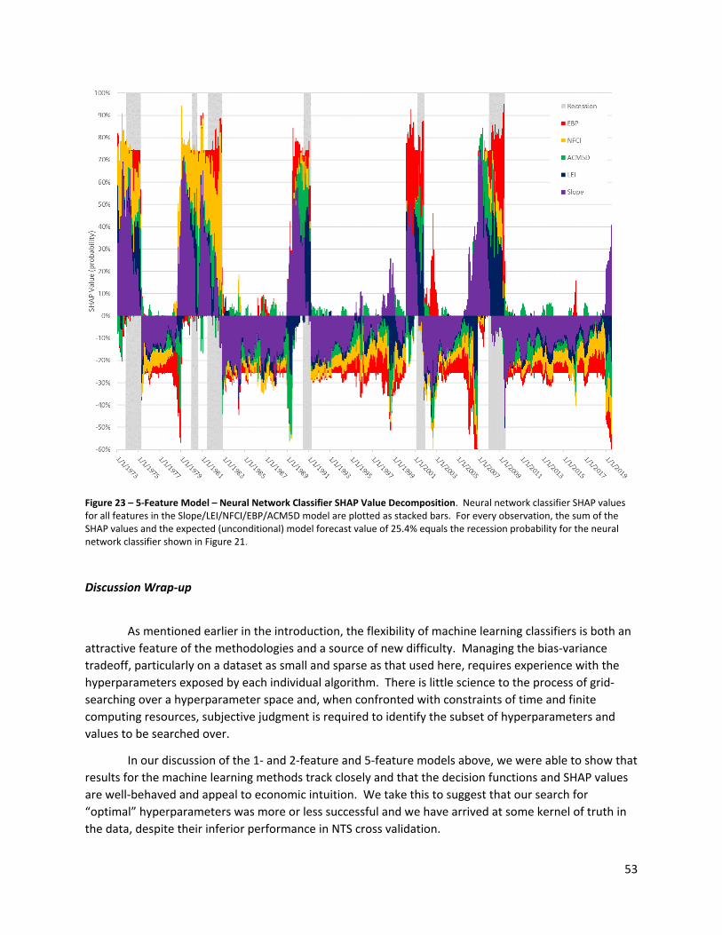
53

Figure 23 – 5-Feature Model – Neural Network Classifier SHAP Value Decomposition. Neural network classifier SHAP values for all features in the Slope/LEI/NFCI/EBP/ACM5D model are plotted as stacked bars. For every observation, the sum of the SHAP values and the expected (unconditional) model forecast value of 25.4% equals the recession probability for the neural network classifier shown in Figure 21.

Discussion Wrap-up

As mentioned earlier in the introduction, the flexibility of machine learning classifiers is both an attractive feature of the methodologies and a source of new difficulty. Managing the bias-variance tradeoff, particularly on a dataset as small and sparse as that used here, requires experience with the hyperparameters exposed by each individual algorithm. There is little science to the process of grid-searching over a hyperparameter space and, when confronted with constraints of time and finite computing resources, subjective judgment is required to identify the subset of hyperparameters and values to be searched over.

In our discussion of the 1- and 2-feature and 5-feature models above, we were able to show that results for the machine learning methods track closely and that the decision functions and SHAP values are well-behaved and appeal to economic intuition. We take this to suggest that our search for “optimal” hyperparameters was more or less successful and we have arrived at some kernel of truth in the data, despite their inferior performance in NTS cross validation.

54

The dataset used in this analysis is sparse, and it is doubtful any method is able to estimate recession probabilities in the tails of the joint feature space well. This fact needs to be considered when assessing any of the figures discussed here. It also highlights the importance of using visualization to supplement the more technical results of the previous section when assessing performance of any binary classifier.

Setting aside these caveats, we might still ask what can be learned from the present discussion that could not be learned from previous studies using probit methods. We summarize the answer to that question as follows:

- In the discussion of the 1-feature Slope models it was shown that the machine learning decision functions are generally steeper and more “non-linear” than the probit decision function. Although perhaps not shown as clearly, this idea can be extended to the 2- and higher- feature models as well. This result should be considered when setting policy.

- Adding a leading indicator of macroeconomic conditions (such as the Conference Board’s

Leading Economic Indicators, or the Philadelphia Fed’s ADS Index) to term spreads greatly improves forecast power at little cost, regardless of the classifier algorithm used for the purpose.

- The Chicago Fed’s NFCI appears to capture some aspects of financial conditions that the

Excess Bond Premium does not. - Rising term premiums may be a subtle forecaster of recession.

We close this discussion with a few comments on the use of machine learning methods in macroeconometrics more generally. Many of the lessons learned here are likely applicable to other studies using the same or similar data.

As we mentioned earlier, the machine learning methods we’ve used are perhaps more appropriately applied to datasets larger than our panel of monthly time-series data. An online retailer deploying these algorithms to build recommender systems, or a credit card company using them to score applicants will collect every minute if not every second new data equivalent in size to the entire 50-year macro/financial panel we’ve used in this paper. It is our opinion that studies employing machine learning methods on new sources of “big” macro and micro data for which most machine learning algorithms are optimized represent an exciting new frontier in econometrics. We also believe that the vast majority of those studies using supervised classification algorithms on “big” data will find that machine learning methods do outperform probit methods along many dimensions, consistent with the growing literature on the subject.

For macroeconometric studies like ours, which employ more traditional monthly and quarterly macro and financial time-series data to (re-)explore parts of the established literature, we believe the challenges posed by the small size and sparse nature of those sets are considerable. In contrast to the large data sets employed by the online retailers and credit card companies of the world, which closely approximate a population and for which standard i.i.d. assumptions often hold, a 50-year time-series of monthly financial market and macroeconomic observations will exhibit not only serial correlation but also multiple structural breaks and, if categorical features like recession are involved, class imbalance as

55

well. It is not clear (to the authors at least) that current technology offers all the tools necessary to contend with these problems.

Complicating our situation further is the fact that the major cross-validation methodologies (such as k-folds, leave-p-out, etc.) commonly used to estimate models using machine learning algorithms and manage the bias-variance tradeoff are also built for application on i.i.d. data, rather than serially correlated time-series data. Though expanding and sliding windows cross-validation are available for the latter type of data, and are likely work well on time-series of daily or higher frequency and many years or decades in length, in cases such as ours these methods presents difficulties.

All this notwithstanding, in managing the bias-variance tradeoff, most of our lessons learned so far are encapsulated in the cross-validation methodology we’ve employed. After many attempts with other strategies, the NTS cross-validation strategy that we have arrived at achieves, we believe, a good balance between training/test set size and validation set size given the constraints posed by serial correlation, class imbalance and structural breaks in the data. It is also sure to provide a very conservative estimate of forecast performance. While allowing hyperparameters to be chosen and out-of-sample forecast error to be estimated simultaneously, the NTS cross-validation strategy:

- Avoids the creation of a test set, to be held out entirely from training for the purpose of out-of-sample forecast error estimation. Holding out the roughly 20-30% of sample data that is commonly needed for this purpose is very costly on small datasets and can result in much higher forecast variance if the time-series available for training is made 20-30% shorter. In cases such as ours, when a positive instance of the indicator does not exist in the most recent 20% of the data, it is perhaps fatal to the study.

- Mitigates class imbalance and problems that arise when sampling unbalanced categorical data, through the use of stratification. Some business cycles are long and some business cycles are short, and likewise some recessions are long and some recessions are short. Stratifying by business cycles ensures that all recession and non-recession periods in the data are sampled from in a balance manner.

- Mitigates some of the problems posed by sampling without replacement from data containing structural breaks, by chaining forward over entire business cycles, rather than data blocks of fixed size. If data blocks of fixed size are used, individual folds of data may end up containing zero instances of a positive indicator, or may bridge business cycles, structural breaks and recession periods awkwardly.

- Simplifies model diagnosis since the samples of forecast error (the outer loop scores) are mapped to specific business cycles. If the forecast error estimate of an outer loop iteration is poor or unusual, the cause is more readily linked back to the idiosyncrasies of the business cycle it is attempting to forecast.

- Avoids data peeking or future leakage, since it is always the case that forecast error is estimated from a test set consisting of observations occurring strictly after all those used to train the classifier.

56

X. Conclusion

Machine learning methods have gained widespread use and acceptance in binary classification problems outside of finance and economics. This paper has investigated their use in forecasting US recessions from term spreads and other financial market and macroeconomic data. To date, most studies examining the problem at hand have used probit methods exclusively.

It has been documented by others in previous work that Treasury term spreads and many of the other financial market and macroeconomic data used in this study (the Excess Bond Premium of Gilchrist and Zakrajsek, the Conference Board’s Leading Economic Index and the Survey of Professional Forecasters, etc.) are forecasters of recession in the US. In this study we show that the Aruoba-Diebold-Scotti (ADS) business conditions index, 6-month changes in ACM 5-year term premiums and the Chicago Fed’s NFCI index also have power to predict US recession.

Although the machine learning methods generally underperform probit regression in NTS cross validation, there is still something to be learned from them. We have shown that machine learning methods are able to capture important features of the joint empirical distribution of Treasury yields and other financial market and macroeconomic data over a recession indicator that probit methods cannot. In particular, machine learning methods, due to their flexibility, are able to capture the “non-linear” nature of those empirical distributions.

We have noted that the data set we have used is very sparse. This presents many challenges in navigating the bias-variance tradeoff when estimating models via ensemble methods. The algorithms we used are designed for application on much larger data sets and even then are prone to over-fit data. Still, in the discussion of our results, we were able to show visually that the results of the machine learning methods (the decision functions) exhibit many of the features of probability distributions and, for practical if not theoretical purposes, can be considered as such. Furthermore, the hyperparameters determined in grid search cross-validation have enabled us to produce results that generally conform to financial and economic intuition. As term spreads flatten, as the credit and financial conditions tighten or macro conditions deteriorate… recession probabilities rise across all of our models and methods. We also showed that the machine learning methods are able to identify characteristics of the empirical distribution of our features over recession that the probit method cannot.

In closing, we offer this analysis (technical, visual and qualitative) to suggest that machine learning methods be included among the standard tools now used to forecast US recession from financial and macroeconomic data.

57

References

1. Adrian, Tobias, Nina Boyarchenko and Domenico Giannone (2016). “Vulnerable Growth,” Federal Reserve Bank of New York Staff Reports, no. 794, September 2016, revised November 2017.

2. Aruoba, S.B., Francis X. Diebold, F.X. and Chiara Scotti (2009). "Real-Time Measurement of Business Conditions," Journal of Business and Economic Statistics, 27:4: 417-27. https://www.philadelphiafed.org/-/media/research-and-data/real-time-center/business-conditions-index/real-time-measurement-of-business-conditions14.pdf?la=en

3. Breiman, Leo, Jerome Friedman, R. A. Olshen, and Charles Stone (1984). Classification and Regression Trees. Belmont: Wadsworth.

4. Breiman, Leo (2001). "Random Forests," Machine Learning. 45 (1): 5–32. https://www.stat.berkeley.edu/~breiman/randomforest2001.pdf

5. Chauvet, Marcelle and Jeremy Piger (2008). “A Comparison of the Real-Time Performance of Business Cycle Dating Methods,” Journal of Business and Economic Statistics, 26(1): 42-49. http://pages.uoregon.edu/jpiger/research/published-papers/chauvet-and-piger_2008_jour.pdf

6. Chauvet, Marcelle and Simon Potter (2005). "Predicting Recessions Using the Yield Curve," Journal of Forecasting 24(2): 77-103. https://doi.org/10.1002/for.932

7. Chen, Tianqi and Carlos Guestrin (2016). “XGBoost: A Scalable Tree Boosting System,” Proceedings of the 22nd ACM SIGKDD International Conference on Knowledge Discovery and Data Mining, August 13-17, 2016, San Francisco, California, USA. https://arxiv.org/pdf/1603.02754.pdf

8. Cochrane, Courtney, “Time Series Nested Cross-Validation,” Towards Data Science, May 18, 2018. https://towardsdatascience.com/time-series-nested-cross-validation-76adba623eb9

9. Cochrane, W. G. (1950). “The comparison of percentages in matched samples,” Biometrika, 37(3/4):256-266.

10. Cohen, Benjamin, Peter Hördahl and Dora Xia (2018). "Term premia: models and some stylised facts," BIS Quarterly Review, Bank for International Settlements, March.

11. Davis, Jesse and Mark Goadrich (2006). “The relationship between Precision-Recall and ROC curves,” Proceedings of the 23rd international conference on Machine learning (ICML '06). ACM, New York, NY, USA, 233-240. DOI: https://doi.org/10.1145/1143844.1143874

12. Dietterich, Thomas G. (1997), “Approximate Statistical Tests for Comparing Supervised Classification Learning Algorithms,” Journal Neural Computation, Volume 10 Issue 7, Oct. 1998, pp. 1895-1923. https://dl.acm.org/citation.cfm?id=303237

13. Dueker, Michael (1997). “Strengthening the Case for the Yield Curve as a Predictor of U.S. Recessions.” Federal Reserve Bank of St. Louis Review, March/April 1997, 79(2): 41-51. https://files.stlouisfed.org/files/htdocs/publications/review/97/03/9703md.pdf

14. Dueker, Michael (2002). "Regime-dependent recession forecasts and the 2001 recession," Review, Federal Reserve Bank of St. Louis, November/December 2002, 84(6): 29-36. https://files.stlouisfed.org/files/htdocs/publications/review/02/11/Dueker.pdf

15. Edwards, A. L. (1948). “Note on the ‘correction for continuity’ in testing the significance of the difference between correlated proportions,” Psychometrika, 13(3):185-187.

16. Engstrom, Eric, and Steve Sharpe (2018). “The Near-Term Forward Yield Spread as a Leading Indicator: A Less Distorted Mirror," Finance and Economics Discussion Series 2018-055. Washington: Board of Governors of the Federal Reserve System, https://doi.org/10.17016/FEDS.2018.055

58

17. Estrella, Arturo and Frederic S. Mishkin (1996). “The Yield Curve as a Predictor of U.S. Recessions,” Current Issues in Economics and Finance, Federal Reserve Bank of New York Research Paper Series, June 1996, 2(7): 1-6. https://ssrn.com/abstract=1001228

18. Estrella, Arturo, and Frederic S. Mishkin (1998). "Predicting U.S. Recessions: Financial Variables as Leading Indicators," The Review of Economics and Statistics, 80(1), 45-61. http://www.jstor.org/stable/2646728

19. Estrella, Arturo, and Mary R. Trubin (2006). “The Yield Curve as a Leading Indicator: Some Practical Issues,” Current Issues in Economics and Finance, Federal Reserve Bank of New York Research Paper Series, July/August 2006, 12(5): 1-8. https://papers.ssrn.com/sol3/papers.cfm?abstract_id=931184

20. Gilchrist, Siman and Egon Zakrajsek (2012). “Credit Spreads and Business Cycle Fluctuations,” American Economic Review, 102(4): 1692-1720. https://pubs.aeaweb.org/doi/pdfplus/10.1257/aer.102.4.1692

21. Gürkaynak, Refet S., Brian Sack, and Jonathan H. Wright (2007), “The U.S. Treasury Yield Curve: 1961 to the Present,” Journal of Monetary Economics, 54(8): 2291–2304. https://www.federalreserve.gov/pubs/feds/2006/200628/200628abs.html

22. Favara, Giovanni, Simon Gilchrist, Kurt F. Lewis, and Egon Zakrajsek (2016). "Recession Risk and the Excess Bond Premium," FEDS Notes. Washington: Board of Governors of the Federal Reserve System, April 8, 2016. http://dx.doi.org/10.17016/2380-7172.1739

23. Favara, Giovanni, Simon Gilchrist, Kurt F. Lewis, and Egon Zakrajsek (2016). "Updating the Recession Risk and the Excess Bond Premium," FEDS Notes. Washington: Board of Governors of the Federal Reserve System, October 6, 2016. https://www.federalreserve.gov/econresdata/notes/feds-notes/2016/updating-the-recession-risk-and-the-excess-bond-premium-20161006.html

24. Fernandez-Delgado, Manuel, Eva Cernadas, Senen Barro, and Dinani Amorim (2014). “Do we Need Hundreds of Classifiers to Solve Real World Classification Problems?” Journal of Machine Learning Research, 15: 3133-3181. http://jmlr.org/papers/volume15/delgado14a/delgado14a.pdf

25. Fornari, Fabio and Wolfgang Lemke (2010). “Predicting Recession Probabilities with Financial Variables Over Multiple Horizons,” European Central Bank, Working Paper Series No. 1255, October 2010. https://ssrn.com/abstract=1685168

26. Fornaro, Paolo (2016). “Forecasting US Recessions with a Large Set of Predictors,” Journal of Forecasting, 35(6): 477–492.

27. Freund, Yoav and Robert Schapire (1999). “A Short Introduction to Boosting,” Journal of Japanese Society for Artificial Intelligence, 14: 771-780. http://www.site.uottawa.ca/~stan/csi5387/boost-tut-ppr.pdf

28. Friedman, Jerome H. (2001). “Greedy function approximation: A gradient boosting machine,” The Annals of Statistics, 29(5):1189-1232. https://projecteuclid.org/euclid.aos/1013203451

29. Friedman, Jerome H. (2002), “Stochastic Gradient Boosting,” Computational Statistics & Data Analysis, 38(4): 367-378.

30. Hastie, T., Tibshirani, R., Friedman, J. H. (2009). The Elements of Statistical Learning. Springer, New York.

31. Holopainen, Markus and Peter Sarlin (2017). “Toward robust early-warning models: A horse race, ensembles and model uncertainty,” Journal of Quantitative Finance, 17(12).

32. Johansson, Peter, and Andrew Meldrum (2018). "Predicting Recession Probabilities Using the Slope of the Yield Curve," FEDS Notes. Washington: Board of Governors of the Federal Reserve System, March 1, 2018, https://doi.org/10.17016/2380-7172.2146

59

33. Joseph, Andreas (2019). “Shapley Regressions: A Framework for Statistical Inference on Machine Learning Models,” Bank of England Working Paper No. 784 (2019), https://ssrn.com/abstract=3351091.

34. Ke, Guolin, Qi Meng, Thomas Finley, Taifeng Wang, Wei Chen, Weidong Ma, Qiwei Ye, Tie-Yan Liu (2017), “Light-GBM: A highly efficient gradient boosting decision tree,” Advances in Neural Information Processing Systems, 30: 3146–3154. https://pdfs.semanticscholar.org/ab2a/5df5c6db9c8fc55117ff71c44f27ba82a087.pdf

35. King, Thomas B. and Levin, Andrew and Perli, Roberto (2007). “Financial Market Perceptions of Recession Risk (October 2007),” Finance and Economics Discussion Series 2007-57. Washington: Board of Governors of the Federal Reserve System. https://ssrn.com/abstract=1049081

36. Kohavi, Ron. (1995). “A Study of Cross-Validation and Bootstrap for Accuracy Estimation and Model Selection,” Proceedings of the 14th International Joint Conference on Artificial intelligence, p.1137-1143, August 20-25, 1995, Montreal, Quebec, Canada. http://ai.stanford.edu/~ronnyk/accEst.pdf

37. Liaw, A. and M. Wiener (2002). Classification and Regression by randomForest. R News 2(3): 18-22. 38. Liu, Weiling and Emanuel Moench (2016). "What Predicts US Recessions?" International Journal of

Forecasting, 32(4): 1138-1150. http://www.sciencedirect.com/science/article/pii/S0169207016300279

39. Loh, Wei-Yin (2014). “Fifty years of classification and regression trees (with discussion),” International Statistical Review, 34: 329-370. https://pdfs.semanticscholar.org/f1c3/683cacc3dc7898f3603753af87565f8ad677.pdf

40. Lundberg, Scott M and Su-In Lee (2017). "A Unified Approach to Interpreting Model Predictions," Advances in Neural Information Processing Systems 30, ed. I. Guyon and U. V. Luxburg and S. Bengio and H. Wallach and R. Fergus and S. Vishwanathan and R. Garnett. http://papers.nips.cc/paper/7062-a-unified-approach-to-interpreting-model-predictions.pdf

41. Lundberg, Scott, Gabriel G. Erion and Su-In Lee (2018). “Consistent Individualized Feature Attribution for Tree Ensembles” https://arxiv.org/abs/1802.03888

42. Mason, Llew, Jonathan Baxter, Peter Bartlett and Marcus Frean. (1999). “Boosting Algorithms as Gradient Descent in Function Space.” https://www.maths.dur.ac.uk/~dma6kp/pdf/face_recognition/Boosting/Mason99AnyboostLong.pdf

43. Mason, Llew, Jonathan Baxter, Peter Bartlett and Marcus Frean. (1999). “Boosting Algorithms as Gradient Descent.” http://papers.nips.cc/paper/1766-boosting-algorithms-as-gradient-descent.pdf

44. McNemar, Q. (1947). “Note on the sampling error of the difference between correlated proportions or percentages,” Psychometrika, 12(2):153-157.

45. Morgan, J.N. and Sonquist, J.A. (1963). “Problems in the analysis of survey data, and a proposal,” Journal of the American Statistical Association, 58 (302): 415–434. https://pdfs.semanticscholar.org/9577/28a4244d3b323e98e351098a0125382f1199.pdf

46. Ng, Serena (2014). “Viewpoint: Boosting Recessions,” Canadian Journal of Economics, 47(1): 1-34. https://doi.org/10.1111/caje.12070

47. Pedregosa et al. (2011), Scikit-learn: Machine Learning in Python, JMLR 12: 2825-2830. 48. Picard, Richard and R. Dennis Cook (1984). “Cross-Validation of Regression Models,” Journal of the

American Statistical Association, 79(387): 575-583. https://www.jstor.org/stable/pdf/2288403.pdf?refreqid=excelsior%3Ab00b387334471ec5185de4462f095bf5

60

49. Raschka, Sebastian (2018). “Model Evaluation, Model Selection, and Algorithm Selection in Machine Learning,” CoRR, abs/1811.12808. https://arxiv.org/abs/1811.12808

50. Ribeiro, Marco Tulio, Sameer Singh and Carlos Guestrin (2016), “’Why Should I Trust You?’: Explaining the Predictions of Any Classifier,” KDD '16 Proceedings of the 22nd ACM SIGKDD International Conference on Knowledge Discovery and Data Mining, 1135-1144

51. Seabold, Skipper, and Josef Perktold (2010). “Statsmodels: Econometric and statistical modeling with python.” Proceedings of the 9th Python in Science Conference. 2010. http://www.statsmodels.org/stable/index.html

52. Shrikumar, Avanti, Peyton Greenside, and Kundaje Anshul (2017). “Learning Important Features Through Propagating Activation Differences,” arXiv:1602.04938

53. Tashman, Leonard J. (2000), “Out-of-sample tests of forecasting accuracy: an analysis and review,” International Journal of Forecasting, 16, pp. 437-450.

54. Varma, Sudhir and Richard Simon (2006), “Bias in error estimation when using cross-validation for model selection,” BMC Bioinformatics, 7(91), February 2006. https://www.researchgate.net/publication/7273753_Bias_in_Error_Estimation_When_Using_Cross-Validation_for_Model_Selection_BMC_Bioinformatics_71_91

55. Wainer, Jacques. (2016). Comparison of 14 different families of classification algorithms on 115 binary datasets. https://arxiv.org/pdf/1606.00930.pdf

56. Westfall, Peter, James F. Troendle and Gene Pennello (2010), “Multiple McNemar Tests,” Biometrics, Vol. 66, No.4, pp. 1185-1191. https://www.jstor.org/stable/40962515

57. Wright, Jonathan H. (2006). “The Yield Curve and Predicting Recessions,” Finance and Economics Discussion Series 2006-7. Washington: Board of Governors of the Federal Reserve System. https://ssrn.com/abstract=899538

61

Appendix – Select Tables

1 Feature 2 Features 3 Features 4 Features 5 Features 6 Features 7 Features 8 Features

ACM5D ADS/NFCI Slope/ADS/ACM5D Slope/ADS/ACM5D/FF Slope/ADS/ACM5D/SP500/SPF Slope/ADS/EBP/ACM5D/SP500/SPF Slope/ADS/NFCI/EBP/ACM5D/SP500/SPF Slope/ADS/NFCI/EBP/ACM5D/SP500/SPF/FF

ADS LEI/NFCI Slope/ADS/EBP Slope/ADS/ACM5D/SP500 Slope/ADS/EBP/ACM5D/SP500 Slope/ADS/NFCI/ACM5D/SP500/SPF Slope/LEI/NFCI/EBP/ACM5D/SP500/SPF Slope/LEI/NFCI/EBP/ACM5D/SP500/SPF/FF

EBP Slope/ACM5D Slope/ADS/FF Slope/ADS/ACM5D/SPF Slope/ADS/EBP/ACM5D/SPF Slope/ADS/NFCI/EBP/ACM5D/SP500

FF Slope/ADS Slope/ADS/NFCI Slope/ADS/EBP/ACM5D Slope/ADS/EBP/SP500/SPF Slope/ADS/NFCI/EBP/ACM5D/SPF

LEI Slope/EBP Slope/ADS/SP500 Slope/ADS/EBP/FF Slope/ADS/NFCI/ACM5D/SP500 Slope/ADS/NFCI/EBP/SP500/SPF

NFCI Slope/FF Slope/ADS/SPF Slope/ADS/EBP/SP500 Slope/ADS/NFCI/ACM5D/SPF Slope/LEI/EBP/ACM5D/SP500/SPF

Slope Slope/LEI Slope/EBP/ACM5D Slope/ADS/EBP/SPF Slope/ADS/NFCI/EBP/ACM5D Slope/LEI/NFCI/ACM5D/SP500/SPF

SP500 Slope/NFCI Slope/EBP/FF Slope/ADS/NFCI/ACM5D Slope/ADS/NFCI/EBP/SP500 Slope/LEI/NFCI/EBP/ACM5D/SP500

SPF Slope/SP500 Slope/EBP/SP500 Slope/ADS/NFCI/EBP Slope/ADS/NFCI/EBP/SPF Slope/LEI/NFCI/EBP/ACM5D/SPF

Slope/SPF Slope/EBP/SPF Slope/ADS/NFCI/FF Slope/ADS/NFCI/SP500/SPF Slope/LEI/NFCI/EBP/SP500/SPF

Slope/LEI/ACM5D Slope/ADS/NFCI/SP500 Slope/LEI/ACM5D/SP500/SPF

Slope/LEI/EBP Slope/ADS/NFCI/SPF Slope/LEI/EBP/ACM5D/SP500

Slope/LEI/FF Slope/ADS/SP500/FF Slope/LEI/EBP/ACM5D/SPF

Slope/LEI/NFCI Slope/ADS/SP500/SPF Slope/LEI/EBP/SP500/SPF

Slope/LEI/SP500 Slope/ADS/SPF/FF Slope/LEI/NFCI/ACM5D/SP500

Slope/LEI/SPF Slope/LEI/ACM5D/FF Slope/LEI/NFCI/ACM5D/SPF

Slope/NFCI/ACM5D Slope/LEI/ACM5D/SP500 Slope/LEI/NFCI/EBP/ACM5D

Slope/NFCI/EBP Slope/LEI/ACM5D/SPF Slope/LEI/NFCI/EBP/SP500

Slope/NFCI/FF Slope/LEI/EBP/ACM5D Slope/LEI/NFCI/EBP/SPF

Slope/NFCI/SP500 Slope/LEI/EBP/FF Slope/LEI/NFCI/SP500/SPF

Slope/NFCI/SPF Slope/LEI/EBP/SP500

Slope/LEI/EBP/SPF

Slope/LEI/NFCI/ACM5D

Slope/LEI/NFCI/EBP

Slope/LEI/NFCI/FF

Slope/LEI/NFCI/SP500

Slope/LEI/NFCI/SPF

Slope/LEI/SP500/FF

Slope/LEI/SP500/SPF

Slope/LEI/SPF/FF

Table 13 – Model Definitions. Definitions for all models used in the paper, named according to the features they contain. Each column collects models with an equal number of features (i.e. the first column contains all 1-feature models). Each of these models is estimated by all six classification algorithms studied in the paper.

62

Rank Feature

Model Probit NN LightGBM XGBoost RF SVM Uncond. 1 7 Slope/LEI/NFCI/EBP/ACM5D/SP500/SPF 0.909 (0.031) 0.931 (0.026) 0.901 (0.031) 0.887 (0.042) 0.911 (0.030) 0.932 (0.026) 0.912 (0.031) 2 6 Slope/LEI/NFCI/EBP/SP500/SPF 0.910 (0.040) 0.912 (0.023) 0.892 (0.040) 0.925 (0.025) 0.903 (0.030) 0.916 (0.034) 0.910 (0.032) 3 5 Slope/LEI/NFCI/EBP/SP500 0.902 (0.045) 0.906 (0.037) 0.913 (0.029) 0.919 (0.029) 0.916 (0.021) 0.899 (0.051) 0.909 (0.035) 4 5 Slope/LEI/NFCI/EBP/ACM5D 0.915 (0.033) 0.915 (0.038) 0.899 (0.035) 0.897 (0.039) 0.907 (0.032) 0.924 (0.027) 0.909 (0.034) 5 5 Slope/LEI/NFCI/ACM5D/SP500 0.904 (0.037) 0.913 (0.031) 0.901 (0.032) 0.898 (0.032) 0.900 (0.033) 0.915 (0.034) 0.905 (0.033) 6 4 Slope/LEI/NFCI/ACM5D 0.920 (0.033) 0.920 (0.028) 0.876 (0.047) 0.903 (0.033) 0.905 (0.030) 0.904 (0.033) 0.905 (0.034) 7 3 Slope/LEI/ACM5D 0.912 (0.039) 0.895 (0.035) 0.906 (0.036) 0.906 (0.027) 0.903 (0.028) 0.906 (0.037) 0.904 (0.034) 8 6 Slope/LEI/NFCI/EBP/ACM5D/SP500 0.875 (0.040) 0.943 (0.023) 0.908 (0.033) 0.894 (0.039) 0.894 (0.035) 0.908 (0.039) 0.904 (0.035) 9 6 Slope/LEI/NFCI/EBP/ACM5D/SPF 0.917 (0.032) 0.906 (0.033) 0.891 (0.038) 0.912 (0.030) 0.874 (0.053) 0.917 (0.032) 0.903 (0.037)

10 5 Slope/LEI/EBP/ACM5D/SPF 0.899 (0.027) 0.887 (0.044) 0.891 (0.035) 0.901 (0.032) 0.911 (0.030) 0.924 (0.031) 0.902 (0.033) 11 5 Slope/LEI/NFCI/ACM5D/SPF 0.906 (0.041) 0.901 (0.035) 0.889 (0.039) 0.922 (0.028) 0.890 (0.039) 0.899 (0.039) 0.901 (0.037) 12 2 Slope/LEI 0.917 (0.023) 0.898 (0.029) 0.893 (0.018) 0.899 (0.027) 0.887 (0.029) 0.905 (0.030) 0.900 (0.026) 13 6 Slope/ADS/NFCI/EBP/ACM5D/SPF 0.954 (0.017) 0.908 (0.037) 0.903 (0.035) 0.893 (0.036) 0.885 (0.037) 0.856 (0.066) 0.900 (0.038) 14 7 Slope/ADS/NFCI/EBP/ACM5D/SP500/SPF 0.899 (0.043) 0.922 (0.034) 0.911 (0.036) 0.864 (0.051) 0.873 (0.040) 0.926 (0.028) 0.899 (0.039) 15 4 Slope/ADS/EBP/ACM5D 0.920 (0.019) 0.855 (0.054) 0.909 (0.032) 0.887 (0.036) 0.900 (0.030) 0.921 (0.020) 0.899 (0.032) 16 5 Slope/ADS/ACM5D/SP500/SPF 0.903 (0.025) 0.903 (0.025) 0.876 (0.042) 0.895 (0.033) 0.902 (0.038) 0.913 (0.033) 0.899 (0.033) 17 4 Slope/LEI/NFCI/SP500 0.896 (0.039) 0.926 (0.024) 0.884 (0.039) 0.921 (0.025) 0.859 (0.042) 0.907 (0.025) 0.899 (0.032) 18 5 Slope/ADS/EBP/ACM5D/SP500 0.895 (0.023) 0.890 (0.046) 0.909 (0.021) 0.914 (0.024) 0.893 (0.028) 0.890 (0.021) 0.899 (0.027) 19 5 Slope/ADS/NFCI/EBP/SP500 0.897 (0.051) 0.904 (0.045) 0.911 (0.036) 0.916 (0.034) 0.867 (0.045) 0.897 (0.040) 0.899 (0.042) 20 4 Slope/LEI/ACM5D/SP500 0.911 (0.036) 0.870 (0.045) 0.896 (0.039) 0.897 (0.024) 0.901 (0.025) 0.909 (0.026) 0.897 (0.032) 21 5 Slope/LEI/NFCI/SP500/SPF 0.896 (0.039) 0.897 (0.031) 0.896 (0.030) 0.928 (0.031) 0.872 (0.040) 0.894 (0.034) 0.897 (0.034) 22 6 Slope/ADS/NFCI/EBP/ACM5D/SP500 0.910 (0.033) 0.908 (0.043) 0.897 (0.034) 0.882 (0.041) 0.859 (0.046) 0.928 (0.032) 0.897 (0.038) 23 6 Slope/LEI/EBP/ACM5D/SP500/SPF 0.922 (0.020) 0.878 (0.048) 0.879 (0.033) 0.898 (0.032) 0.905 (0.029) 0.901 (0.029) 0.897 (0.032) 24 6 Slope/LEI/NFCI/ACM5D/SP500/SPF 0.895 (0.041) 0.903 (0.033) 0.904 (0.032) 0.869 (0.055) 0.904 (0.034) 0.905 (0.031) 0.897 (0.038) 25 3 Slope/LEI/SP500 0.903 (0.028) 0.888 (0.033) 0.896 (0.026) 0.903 (0.029) 0.880 (0.025) 0.910 (0.020) 0.897 (0.027) 26 4 Slope/ADS/SP500/SPF 0.902 (0.024) 0.902 (0.014) 0.903 (0.030) 0.901 (0.028) 0.884 (0.031) 0.887 (0.026) 0.896 (0.026) 27 4 Slope/ADS/NFCI/EBP 0.898 (0.044) 0.897 (0.031) 0.889 (0.050) 0.904 (0.032) 0.906 (0.038) 0.884 (0.046) 0.896 (0.040) 28 6 Slope/ADS/EBP/ACM5D/SP500/SPF 0.899 (0.027) 0.873 (0.044) 0.920 (0.016) 0.901 (0.031) 0.876 (0.037) 0.908 (0.025) 0.896 (0.030) 29 5 Slope/LEI/ACM5D/SP500/SPF 0.903 (0.046) 0.889 (0.029) 0.876 (0.044) 0.898 (0.032) 0.886 (0.039) 0.921 (0.022) 0.896 (0.035) 30 3 Slope/LEI/SPF 0.920 (0.027) 0.879 (0.027) 0.870 (0.040) 0.908 (0.024) 0.884 (0.040) 0.908 (0.027) 0.895 (0.031) 31 5 Slope/ADS/EBP/ACM5D/SPF 0.902 (0.036) 0.872 (0.064) 0.915 (0.021) 0.903 (0.027) 0.872 (0.041) 0.904 (0.026) 0.895 (0.036) 32 5 Slope/LEI/EBP/ACM5D/SP500 0.877 (0.035) 0.911 (0.024) 0.884 (0.032) 0.909 (0.028) 0.900 (0.026) 0.883 (0.037) 0.894 (0.030) 33 5 Slope/ADS/NFCI/EBP/ACM5D 0.931 (0.036) 0.897 (0.034) 0.914 (0.029) 0.885 (0.041) 0.869 (0.049) 0.866 (0.055) 0.894 (0.041) 34 3 Slope/ADS/SP500 0.891 (0.021) 0.912 (0.013) 0.908 (0.028) 0.873 (0.029) 0.885 (0.037) 0.894 (0.024) 0.894 (0.025) 35 5 Slope/ADS/NFCI/EBP/SPF 0.901 (0.042) 0.888 (0.038) 0.903 (0.044) 0.897 (0.044) 0.921 (0.029) 0.851 (0.066) 0.894 (0.044) 36 4 Slope/LEI/ACM5D/SPF 0.911 (0.039) 0.874 (0.042) 0.916 (0.021) 0.886 (0.039) 0.905 (0.030) 0.869 (0.060) 0.893 (0.038) 37 8 Slope/LEI/NFCI/EBP/ACM5D/SP500/SPF/FF 0.894 (0.047) 0.906 (0.045) 0.889 (0.041) 0.862 (0.059) 0.898 (0.034) 0.907 (0.042) 0.893 (0.045) 38 5 Slope/ADS/NFCI/ACM5D/SP500 0.902 (0.046) 0.891 (0.037) 0.893 (0.036) 0.867 (0.048) 0.888 (0.037) 0.915 (0.031) 0.893 (0.039) 39 6 Slope/ADS/NFCI/EBP/SP500/SPF 0.889 (0.046) 0.910 (0.046) 0.886 (0.039) 0.921 (0.025) 0.855 (0.046) 0.892 (0.037) 0.892 (0.040) 40 5 Slope/ADS/NFCI/ACM5D/SPF 0.918 (0.031) 0.887 (0.038) 0.900 (0.033) 0.864 (0.051) 0.897 (0.041) 0.885 (0.036) 0.892 (0.039) 41 5 Slope/LEI/EBP/SP500/SPF 0.873 (0.042) 0.872 (0.035) 0.895 (0.029) 0.906 (0.026) 0.899 (0.035) 0.900 (0.033) 0.891 (0.033) 42 4 Slope/LEI/EBP/ACM5D 0.883 (0.033) 0.848 (0.068) 0.890 (0.035) 0.907 (0.033) 0.888 (0.038) 0.925 (0.030) 0.890 (0.039) 43 3 Slope/ADS/EBP 0.875 (0.032) 0.905 (0.031) 0.877 (0.042) 0.898 (0.023) 0.878 (0.042) 0.906 (0.032) 0.890 (0.034) 44 6 Slope/ADS/NFCI/ACM5D/SP500/SPF 0.942 (0.020) 0.874 (0.045) 0.887 (0.036) 0.867 (0.049) 0.873 (0.043) 0.895 (0.030) 0.890 (0.037) 45 4 Slope/ADS/ACM5D/SP500 0.893 (0.026) 0.872 (0.030) 0.882 (0.034) 0.887 (0.034) 0.890 (0.032) 0.915 (0.034) 0.890 (0.032) 46 4 Slope/LEI/NFCI/SPF 0.902 (0.038) 0.895 (0.029) 0.897 (0.030) 0.907 (0.032) 0.868 (0.046) 0.870 (0.046) 0.890 (0.037) 47 5 Slope/LEI/NFCI/EBP/SPF 0.895 (0.049) 0.874 (0.032) 0.916 (0.034) 0.915 (0.029) 0.897 (0.038) 0.841 (0.055) 0.890 (0.039) 48 4 Slope/LEI/NFCI/EBP 0.900 (0.043) 0.847 (0.034) 0.894 (0.037) 0.912 (0.033) 0.895 (0.036) 0.888 (0.039) 0.889 (0.037) 49 4 Slope/ADS/NFCI/SP500 0.896 (0.042) 0.890 (0.037) 0.893 (0.036) 0.880 (0.039) 0.877 (0.052) 0.895 (0.033) 0.889 (0.040) 50 5 Slope/ADS/EBP/SP500/SPF 0.880 (0.041) 0.876 (0.022) 0.903 (0.029) 0.903 (0.018) 0.858 (0.029) 0.906 (0.032) 0.888 (0.029) 51 3 Slope/ADS/ACM5D 0.895 (0.030) 0.882 (0.033) 0.871 (0.057) 0.878 (0.035) 0.878 (0.034) 0.922 (0.024) 0.888 (0.036) 52 4 Slope/LEI/SP500/SPF 0.902 (0.028) 0.897 (0.030) 0.876 (0.033) 0.862 (0.040) 0.891 (0.026) 0.896 (0.034) 0.887 (0.032) 53 2 LEI/NFCI 0.910 (0.029) 0.891 (0.036) 0.887 (0.024) 0.870 (0.044) 0.864 (0.039) 0.901 (0.028) 0.887 (0.033) 54 3 Slope/ADS/NFCI 0.901 (0.042) 0.869 (0.052) 0.900 (0.037) 0.866 (0.050) 0.888 (0.038) 0.893 (0.040) 0.886 (0.043) 55 4 Slope/LEI/EBP/SP500 0.881 (0.037) 0.875 (0.031) 0.879 (0.011) 0.912 (0.023) 0.881 (0.030) 0.886 (0.034) 0.886 (0.028) 56 4 Slope/ADS/EBP/SP500 0.877 (0.033) 0.890 (0.033) 0.879 (0.033) 0.899 (0.020) 0.892 (0.045) 0.876 (0.034) 0.885 (0.033) 57 4 Slope/ADS/NFCI/SPF 0.899 (0.042) 0.862 (0.053) 0.895 (0.037) 0.883 (0.039) 0.883 (0.037) 0.885 (0.047) 0.885 (0.043) 58 4 Slope/ADS/EBP/SPF 0.874 (0.038) 0.862 (0.039) 0.890 (0.030) 0.922 (0.027) 0.882 (0.028) 0.872 (0.041) 0.884 (0.034) 59 5 Slope/ADS/NFCI/SP500/SPF 0.898 (0.043) 0.891 (0.037) 0.913 (0.030) 0.859 (0.046) 0.862 (0.047) 0.878 (0.024) 0.883 (0.038) 60 4 Slope/LEI/EBP/SPF 0.884 (0.044) 0.833 (0.047) 0.894 (0.020) 0.892 (0.032) 0.899 (0.028) 0.887 (0.050) 0.882 (0.037) 61 3 Slope/ADS/SPF 0.918 (0.018) 0.882 (0.037) 0.853 (0.058) 0.869 (0.041) 0.870 (0.035) 0.890 (0.029) 0.880 (0.036) 62 4 Slope/ADS/ACM5D/SPF 0.919 (0.020) 0.851 (0.061) 0.856 (0.058) 0.882 (0.037) 0.868 (0.037) 0.898 (0.029) 0.879 (0.040) 63 4 Slope/ADS/NFCI/ACM5D 0.914 (0.033) 0.867 (0.043) 0.846 (0.058) 0.883 (0.044) 0.874 (0.041) 0.888 (0.037) 0.879 (0.043) 64 3 Slope/LEI/NFCI 0.905 (0.035) 0.861 (0.050) 0.893 (0.035) 0.869 (0.052) 0.860 (0.037) 0.879 (0.039) 0.878 (0.041) 65 1 LEI 0.878 (0.033) 0.886 (0.036) 0.867 (0.025) 0.870 (0.031) 0.862 (0.025) 0.900 (0.037) 0.877 (0.031) 66 2 Slope/ADS 0.889 (0.031) 0.888 (0.029) 0.864 (0.042) 0.870 (0.041) 0.868 (0.040) 0.881 (0.027) 0.877 (0.035) 67 3 Slope/LEI/EBP 0.868 (0.040) 0.883 (0.039) 0.891 (0.024) 0.884 (0.035) 0.877 (0.038) 0.852 (0.064) 0.876 (0.040) 68 8 Slope/ADS/NFCI/EBP/ACM5D/SP500/SPF/FF 0.896 (0.038) 0.910 (0.040) 0.868 (0.043) 0.831 (0.063) 0.851 (0.049) 0.893 (0.039) 0.875 (0.045) 69 12 Large(12-Variable) 0.906 (0.043) 0.868 (0.047) 0.905 (0.038) 0.844 (0.045) 0.897 (0.029) 0.793 (0.079) 0.869 (0.047) 70 4 Slope/LEI/SP500/FF 0.902 (0.039) 0.892 (0.042) 0.894 (0.042) 0.854 (0.057) 0.848 (0.054) 0.821 (0.086) 0.869 (0.053) 71 2 ADS/NFCI 0.881 (0.036) 0.864 (0.046) 0.863 (0.032) 0.865 (0.031) 0.876 (0.041) 0.861 (0.047) 0.868 (0.039) 72 4 Slope/LEI/ACM5D/FF 0.920 (0.030) 0.894 (0.020) 0.871 (0.049) 0.858 (0.057) 0.864 (0.059) 0.791 (0.053) 0.866 (0.045) 73 3 Slope/EBP/SPF 0.888 (0.048) 0.883 (0.057) 0.857 (0.051) 0.850 (0.038) 0.824 (0.053) 0.878 (0.044) 0.863 (0.048) 74 4 Slope/ADS/ACM5D/FF 0.888 (0.044) 0.877 (0.055) 0.865 (0.044) 0.866 (0.044) 0.850 (0.051) 0.828 (0.089) 0.862 (0.054) 75 4 Slope/ADS/SP500/FF 0.880 (0.042) 0.880 (0.049) 0.871 (0.048) 0.863 (0.044) 0.829 (0.064) 0.833 (0.065) 0.859 (0.052) 76 3 Slope/NFCI/EBP 0.887 (0.055) 0.898 (0.037) 0.839 (0.062) 0.834 (0.053) 0.828 (0.052) 0.866 (0.046) 0.859 (0.051) 77 3 Slope/EBP/ACM5D 0.900 (0.031) 0.853 (0.065) 0.845 (0.044) 0.836 (0.051) 0.824 (0.050) 0.887 (0.034) 0.858 (0.046) 78 4 Slope/LEI/NFCI/FF 0.893 (0.044) 0.894 (0.036) 0.877 (0.047) 0.879 (0.044) 0.886 (0.039) 0.716 (0.119) 0.857 (0.055) 79 2 Slope/SPF 0.879 (0.051) 0.879 (0.034) 0.835 (0.062) 0.858 (0.051) 0.827 (0.048) 0.843 (0.038) 0.853 (0.047) 80 3 Slope/NFCI/SPF 0.853 (0.052) 0.831 (0.071) 0.886 (0.040) 0.834 (0.058) 0.846 (0.052) 0.870 (0.045) 0.853 (0.053) 81 3 Slope/NFCI/SP500 0.859 (0.052) 0.849 (0.057) 0.857 (0.039) 0.846 (0.053) 0.841 (0.050) 0.839 (0.057) 0.848 (0.052) 82 1 NFCI 0.847 (0.048) 0.851 (0.046) 0.863 (0.050) 0.844 (0.052) 0.839 (0.052) 0.834 (0.058) 0.846 (0.051) 83 4 Slope/ADS/NFCI/FF 0.887 (0.033) 0.849 (0.037) 0.884 (0.041) 0.855 (0.050) 0.855 (0.047) 0.748 (0.146) 0.846 (0.059) 84 3 Slope/LEI/FF 0.887 (0.045) 0.911 (0.039) 0.832 (0.081) 0.857 (0.057) 0.847 (0.054) 0.738 (0.127) 0.845 (0.067) 85 3 Slope/NFCI/ACM5D 0.874 (0.046) 0.835 (0.061) 0.858 (0.045) 0.810 (0.064) 0.830 (0.055) 0.852 (0.047) 0.843 (0.053) 86 2 Slope/NFCI 0.845 (0.061) 0.865 (0.053) 0.855 (0.058) 0.814 (0.062) 0.809 (0.061) 0.861 (0.048) 0.841 (0.057) 87 4 Slope/ADS/SPF/FF 0.792 (0.102) 0.897 (0.037) 0.851 (0.050) 0.863 (0.043) 0.840 (0.058) 0.777 (0.101) 0.837 (0.065) 88 3 Slope/ADS/FF 0.865 (0.046) 0.870 (0.052) 0.858 (0.043) 0.826 (0.068) 0.820 (0.070) 0.779 (0.112) 0.836 (0.065)

63

89 3 Slope/EBP/SP500 0.853 (0.051) 0.838 (0.058) 0.798 (0.054) 0.810 (0.039) 0.811 (0.050) 0.837 (0.057) 0.824 (0.052) 90 4 Slope/ADS/EBP/FF 0.831 (0.084) 0.870 (0.047) 0.781 (0.113) 0.845 (0.049) 0.828 (0.072) 0.790 (0.086) 0.824 (0.075) 91 1 SPF 0.822 (0.090) 0.822 (0.090) 0.824 (0.091) 0.806 (0.107) 0.806 (0.107) 0.809 (0.099) 0.815 (0.097) 92 2 Slope/EBP 0.859 (0.044) 0.829 (0.043) 0.794 (0.057) 0.822 (0.049) 0.792 (0.053) 0.788 (0.063) 0.814 (0.052) 93 4 Slope/LEI/SPF/FF 0.816 (0.101) 0.861 (0.059) 0.871 (0.044) 0.860 (0.057) 0.864 (0.045) 0.612 (0.091) 0.814 (0.066) 94 4 Slope/LEI/EBP/FF 0.847 (0.082) 0.822 (0.083) 0.798 (0.111) 0.889 (0.040) 0.843 (0.061) 0.627 (0.072) 0.804 (0.075) 95 2 Slope/SP500 0.799 (0.060) 0.807 (0.056) 0.772 (0.053) 0.788 (0.056) 0.790 (0.052) 0.824 (0.058) 0.797 (0.056) 96 1 ADS 0.776 (0.088) 0.796 (0.067) 0.792 (0.087) 0.778 (0.088) 0.775 (0.089) 0.844 (0.068) 0.794 (0.081) 97 2 Slope/ACM5D 0.836 (0.074) 0.804 (0.065) 0.763 (0.075) 0.809 (0.065) 0.768 (0.069) 0.779 (0.070) 0.793 (0.070) 98 3 Slope/NFCI/FF 0.836 (0.036) 0.842 (0.025) 0.795 (0.051) 0.792 (0.050) 0.787 (0.062) 0.664 (0.112) 0.786 (0.056) 99 1 Slope 0.800 (0.067) 0.753 (0.070) 0.744 (0.070) 0.807 (0.065) 0.773 (0.081) 0.768 (0.072) 0.774 (0.071)

100 20 Large(20-Variable) 0.749 (0.142) 0.732 (0.177) 0.800 (0.095) 0.867 (0.039) 0.710 (0.155) 0.713 (0.169) 0.762 (0.130) 101 3 Slope/EBP/FF 0.798 (0.109) 0.806 (0.096) 0.765 (0.102) 0.775 (0.074) 0.765 (0.080) 0.624 (0.076) 0.755 (0.089) 102 1 EBP 0.743 (0.166) 0.751 (0.158) 0.746 (0.144) 0.765 (0.130) 0.747 (0.135) 0.743 (0.164) 0.749 (0.149) 103 1 SP500 0.723 (0.141) 0.691 (0.154) 0.652 (0.158) 0.684 (0.166) 0.681 (0.166) 0.695 (0.176) 0.688 (0.160) 104 2 Slope/FF 0.797 (0.086) 0.740 (0.139) 0.706 (0.113) 0.562 (0.126) 0.483 (0.120) 0.734 (0.106) 0.670 (0.115) 105 1 ACM5D 0.687 (0.127) 0.680 (0.122) 0.663 (0.131) 0.637 (0.150) 0.666 (0.133) 0.685 (0.174) 0.670 (0.140) 106 1 FF 0.746 (0.114) 0.551 (0.132) 0.734 (0.124) 0.558 (0.135) 0.558 (0.135) 0.570 (0.150) 0.619 (0.132)

Unconditional 0.878 (0.047) 0.867 (0.048) 0.865 (0.047) 0.863 (0.046) 0.854 (0.049) 0.854 (0.054) 0.864 (0.048)

Table 14 – Nested Time-Series Cross-Validation Results. Mean out-of-sample forecast accuracy for each model and classifier estimated using nested time-series cross-validation is reported in the table above. Standard errors of the accuracy estimate are in parenthesis. The top 5 individual classifiers are highlighted in dark orange. The best class of nested models is highlighted in light orange.

Rank Feature

Model Probit NN LightGBM XGBoost RF SVM Uncond 1 6 Slope/ADS/NFCI/EBP/ACM5D/SPF 0.950 (0.015) 0.952 (0.010) 0.975 (0.010) 0.952 (0.018) 0.950 (0.013) 0.964 (0.006) 0.957 (0.012) 2 6 Slope/LEI/NFCI/EBP/ACM5D/SPF 0.946 (0.016) 0.966 (0.012) 0.968 (0.007) 0.946 (0.015) 0.955 (0.010) 0.957 (0.008) 0.956 (0.011) 3 7 Slope/ADS/NFCI/EBP/ACM5D/SP500/SPF 0.934 (0.010) 0.955 (0.009) 0.968 (0.010) 0.955 (0.016) 0.948 (0.015) 0.959 (0.007) 0.953 (0.011) 4 8 Slope/LEI/NFCI/EBP/ACM5D/SP500/SPF/FF 0.941 (0.011) 0.948 (0.009) 0.968 (0.007) 0.950 (0.014) 0.950 (0.016) 0.957 (0.013) 0.952 (0.012) 5 12 Large(12-Variable) 0.930 (0.011) 0.950 (0.010) 0.971 (0.011) 0.957 (0.013) 0.961 (0.011) 0.946 (0.013) 0.952 (0.011) 6 6 Slope/ADS/NFCI/ACM5D/SP500/SPF 0.946 (0.013) 0.946 (0.009) 0.961 (0.014) 0.952 (0.015) 0.952 (0.014) 0.957 (0.014) 0.952 (0.013) 7 5 Slope/ADS/EBP/ACM5D/SPF 0.939 (0.012) 0.959 (0.011) 0.957 (0.012) 0.957 (0.011) 0.948 (0.006) 0.952 (0.007) 0.952 (0.010) 8 5 Slope/LEI/NFCI/EBP/ACM5D 0.943 (0.015) 0.948 (0.009) 0.953 (0.010) 0.948 (0.011) 0.950 (0.009) 0.964 (0.008) 0.951 (0.010) 9 7 Slope/LEI/NFCI/EBP/ACM5D/SP500/SPF 0.919 (0.018) 0.959 (0.010) 0.962 (0.011) 0.943 (0.012) 0.952 (0.012) 0.964 (0.011) 0.950 (0.012)

10 20 Large(20-Variable) 0.889 (0.028) 0.957 (0.010) 0.975 (0.008) 0.959 (0.014) 0.968 (0.007) 0.950 (0.010) 0.950 (0.013) 11 8 Slope/ADS/NFCI/EBP/ACM5D/SP500/SPF/FF 0.932 (0.019) 0.946 (0.018) 0.971 (0.011) 0.957 (0.014) 0.950 (0.013) 0.944 (0.014) 0.950 (0.015) 12 5 Slope/ADS/NFCI/ACM5D/SPF 0.939 (0.012) 0.943 (0.011) 0.966 (0.010) 0.943 (0.021) 0.952 (0.010) 0.950 (0.012) 0.949 (0.013) 13 5 Slope/LEI/NFCI/ACM5D/SPF 0.946 (0.008) 0.948 (0.007) 0.957 (0.011) 0.948 (0.011) 0.948 (0.011) 0.948 (0.015) 0.949 (0.010) 14 4 Slope/ADS/EBP/ACM5D 0.941 (0.010) 0.950 (0.011) 0.948 (0.008) 0.952 (0.012) 0.943 (0.013) 0.955 (0.010) 0.948 (0.011) 15 5 Slope/ADS/NFCI/EBP/ACM5D 0.946 (0.014) 0.946 (0.012) 0.955 (0.010) 0.952 (0.018) 0.943 (0.014) 0.948 (0.015) 0.948 (0.014) 16 6 Slope/ADS/EBP/ACM5D/SP500/SPF 0.925 (0.011) 0.946 (0.015) 0.959 (0.018) 0.959 (0.012) 0.950 (0.010) 0.948 (0.006) 0.948 (0.012) 17 5 Slope/LEI/EBP/ACM5D/SPF 0.941 (0.013) 0.946 (0.013) 0.957 (0.011) 0.941 (0.009) 0.943 (0.008) 0.952 (0.007) 0.947 (0.010) 18 4 Slope/LEI/EBP/ACM5D 0.932 (0.011) 0.953 (0.006) 0.959 (0.008) 0.946 (0.014) 0.939 (0.010) 0.950 (0.009) 0.946 (0.010) 19 6 Slope/LEI/EBP/ACM5D/SP500/SPF 0.943 (0.013) 0.950 (0.009) 0.950 (0.008) 0.946 (0.011) 0.943 (0.008) 0.946 (0.012) 0.946 (0.010) 20 6 Slope/ADS/NFCI/EBP/ACM5D/SP500 0.932 (0.008) 0.950 (0.009) 0.955 (0.014) 0.955 (0.014) 0.939 (0.013) 0.948 (0.008) 0.946 (0.011) 21 6 Slope/LEI/NFCI/EBP/ACM5D/SP500 0.930 (0.020) 0.946 (0.013) 0.955 (0.009) 0.943 (0.010) 0.950 (0.009) 0.955 (0.010) 0.946 (0.012) 22 6 Slope/LEI/NFCI/ACM5D/SP500/SPF 0.934 (0.010) 0.946 (0.013) 0.950 (0.012) 0.946 (0.010) 0.946 (0.011) 0.953 (0.015) 0.946 (0.012) 23 4 Slope/LEI/NFCI/ACM5D 0.950 (0.015) 0.948 (0.013) 0.943 (0.010) 0.943 (0.012) 0.943 (0.007) 0.943 (0.009) 0.945 (0.011) 24 4 Slope/ADS/NFCI/EBP 0.937 (0.012) 0.952 (0.009) 0.948 (0.012) 0.948 (0.017) 0.937 (0.014) 0.950 (0.011) 0.945 (0.012) 25 5 Slope/ADS/NFCI/EBP/SPF 0.930 (0.013) 0.948 (0.009) 0.959 (0.011) 0.941 (0.021) 0.946 (0.012) 0.948 (0.009) 0.945 (0.013) 26 4 Slope/ADS/ACM5D/FF 0.937 (0.008) 0.934 (0.008) 0.946 (0.013) 0.959 (0.012) 0.946 (0.009) 0.941 (0.007) 0.944 (0.009) 27 4 Slope/LEI/ACM5D/FF 0.939 (0.011) 0.939 (0.012) 0.950 (0.008) 0.946 (0.015) 0.946 (0.010) 0.941 (0.015) 0.943 (0.012) 28 5 Slope/LEI/NFCI/EBP/SPF 0.939 (0.015) 0.943 (0.008) 0.957 (0.008) 0.941 (0.020) 0.939 (0.012) 0.934 (0.013) 0.942 (0.013) 29 4 Slope/ADS/ACM5D/SPF 0.916 (0.016) 0.952 (0.015) 0.941 (0.015) 0.943 (0.017) 0.952 (0.010) 0.946 (0.010) 0.942 (0.014) 30 6 Slope/ADS/NFCI/EBP/SP500/SPF 0.930 (0.018) 0.939 (0.014) 0.957 (0.010) 0.946 (0.017) 0.943 (0.015) 0.937 (0.012) 0.942 (0.014) 31 5 Slope/ADS/NFCI/ACM5D/SP500 0.939 (0.014) 0.932 (0.013) 0.952 (0.007) 0.946 (0.014) 0.937 (0.015) 0.939 (0.009) 0.941 (0.012) 32 4 Slope/ADS/NFCI/FF 0.925 (0.015) 0.953 (0.007) 0.941 (0.006) 0.948 (0.011) 0.937 (0.013) 0.939 (0.008) 0.940 (0.010) 33 4 Slope/LEI/NFCI/EBP 0.937 (0.015) 0.943 (0.008) 0.943 (0.007) 0.937 (0.011) 0.939 (0.008) 0.941 (0.004) 0.940 (0.009) 34 5 Slope/ADS/EBP/ACM5D/SP500 0.923 (0.009) 0.943 (0.018) 0.946 (0.009) 0.948 (0.014) 0.934 (0.013) 0.946 (0.014) 0.940 (0.013) 35 5 Slope/LEI/NFCI/ACM5D/SP500 0.907 (0.020) 0.941 (0.012) 0.952 (0.012) 0.946 (0.013) 0.948 (0.009) 0.944 (0.017) 0.940 (0.014) 36 4 Slope/ADS/NFCI/SPF 0.923 (0.016) 0.934 (0.009) 0.952 (0.014) 0.937 (0.020) 0.941 (0.016) 0.946 (0.008) 0.939 (0.014) 37 4 Slope/ADS/NFCI/ACM5D 0.937 (0.009) 0.930 (0.007) 0.941 (0.015) 0.946 (0.014) 0.937 (0.011) 0.941 (0.007) 0.939 (0.010) 38 5 Slope/LEI/EBP/ACM5D/SP500 0.934 (0.013) 0.939 (0.014) 0.948 (0.008) 0.937 (0.012) 0.934 (0.011) 0.939 (0.012) 0.938 (0.012) 39 5 Slope/LEI/NFCI/EBP/SP500 0.937 (0.015) 0.930 (0.012) 0.950 (0.008) 0.934 (0.010) 0.939 (0.008) 0.941 (0.012) 0.938 (0.011) 40 5 Slope/ADS/NFCI/EBP/SP500 0.934 (0.013) 0.932 (0.019) 0.943 (0.010) 0.946 (0.017) 0.937 (0.014) 0.937 (0.012) 0.938 (0.014) 41 3 Slope/ADS/NFCI 0.923 (0.016) 0.943 (0.011) 0.934 (0.013) 0.943 (0.013) 0.939 (0.012) 0.943 (0.013) 0.938 (0.013) 42 5 Slope/ADS/ACM5D/SP500/SPF 0.921 (0.018) 0.923 (0.016) 0.943 (0.012) 0.946 (0.019) 0.948 (0.008) 0.939 (0.014) 0.937 (0.014) 43 6 Slope/LEI/NFCI/EBP/SP500/SPF 0.928 (0.016) 0.930 (0.014) 0.952 (0.012) 0.939 (0.016) 0.939 (0.018) 0.932 (0.011) 0.937 (0.015) 44 4 Slope/LEI/NFCI/FF 0.925 (0.015) 0.932 (0.015) 0.939 (0.011) 0.937 (0.019) 0.943 (0.017) 0.939 (0.015) 0.936 (0.015) 45 5 Slope/ADS/NFCI/SP500/SPF 0.925 (0.015) 0.921 (0.014) 0.955 (0.006) 0.941 (0.018) 0.946 (0.012) 0.923 (0.017) 0.935 (0.014) 46 4 Slope/ADS/EBP/SPF 0.909 (0.013) 0.932 (0.016) 0.946 (0.010) 0.941 (0.019) 0.948 (0.013) 0.934 (0.021) 0.935 (0.015) 47 3 Slope/EBP/SPF 0.923 (0.015) 0.932 (0.011) 0.943 (0.010) 0.932 (0.017) 0.946 (0.010) 0.932 (0.016) 0.935 (0.013) 48 4 Slope/LEI/EBP/SPF 0.930 (0.015) 0.930 (0.014) 0.943 (0.016) 0.932 (0.017) 0.941 (0.014) 0.932 (0.018) 0.935 (0.016) 49 4 Slope/ADS/SPF/FF 0.909 (0.016) 0.937 (0.014) 0.939 (0.010) 0.939 (0.017) 0.948 (0.012) 0.932 (0.014) 0.934 (0.014) 50 4 Slope/ADS/EBP/FF 0.923 (0.014) 0.928 (0.013) 0.941 (0.012) 0.941 (0.015) 0.941 (0.017) 0.930 (0.019) 0.934 (0.015) 51 4 Slope/ADS/NFCI/SP500 0.923 (0.014) 0.937 (0.016) 0.943 (0.015) 0.939 (0.011) 0.928 (0.016) 0.932 (0.012) 0.934 (0.014) 52 3 Slope/LEI/NFCI 0.919 (0.013) 0.939 (0.015) 0.939 (0.014) 0.932 (0.018) 0.937 (0.011) 0.937 (0.013) 0.934 (0.014) 53 4 Slope/LEI/NFCI/SPF 0.919 (0.013) 0.943 (0.008) 0.941 (0.009) 0.932 (0.015) 0.941 (0.012) 0.923 (0.008) 0.933 (0.011) 54 4 Slope/LEI/SPF/FF 0.928 (0.013) 0.925 (0.020) 0.946 (0.011) 0.930 (0.020) 0.943 (0.015) 0.928 (0.008) 0.933 (0.014) 55 4 Slope/LEI/EBP/FF 0.925 (0.013) 0.923 (0.015) 0.946 (0.007) 0.934 (0.019) 0.937 (0.016) 0.934 (0.017) 0.933 (0.014) 56 4 Slope/LEI/ACM5D/SPF 0.923 (0.016) 0.925 (0.006) 0.941 (0.008) 0.937 (0.017) 0.941 (0.010) 0.930 (0.009) 0.933 (0.011) 57 5 Slope/LEI/EBP/SP500/SPF 0.925 (0.015) 0.923 (0.013) 0.943 (0.016) 0.932 (0.016) 0.939 (0.011) 0.932 (0.016) 0.932 (0.014) 58 3 Slope/ADS/FF 0.905 (0.015) 0.934 (0.012) 0.928 (0.018) 0.943 (0.015) 0.948 (0.010) 0.934 (0.015) 0.932 (0.014) 59 3 Slope/LEI/FF 0.928 (0.013) 0.937 (0.014) 0.934 (0.010) 0.934 (0.024) 0.941 (0.016) 0.916 (0.015) 0.932 (0.015) 60 5 Slope/LEI/ACM5D/SP500/SPF 0.925 (0.015) 0.923 (0.016) 0.946 (0.008) 0.934 (0.013) 0.939 (0.008) 0.921 (0.013) 0.931 (0.012) 61 3 Slope/LEI/ACM5D 0.932 (0.008) 0.916 (0.009) 0.934 (0.009) 0.925 (0.015) 0.939 (0.012) 0.937 (0.010) 0.931 (0.010) 62 5 Slope/ADS/EBP/SP500/SPF 0.894 (0.022) 0.916 (0.026) 0.948 (0.017) 0.943 (0.017) 0.943 (0.012) 0.930 (0.022) 0.929 (0.019)

64

63 3 Slope/ADS/ACM5D 0.912 (0.014) 0.919 (0.014) 0.932 (0.013) 0.941 (0.016) 0.930 (0.015) 0.934 (0.008) 0.928 (0.013) 64 4 Slope/LEI/ACM5D/SP500 0.923 (0.011) 0.921 (0.018) 0.939 (0.012) 0.930 (0.011) 0.937 (0.012) 0.919 (0.019) 0.928 (0.014) 65 4 Slope/ADS/ACM5D/SP500 0.914 (0.017) 0.925 (0.014) 0.930 (0.015) 0.946 (0.016) 0.930 (0.020) 0.921 (0.018) 0.928 (0.016) 66 5 Slope/LEI/NFCI/SP500/SPF 0.921 (0.013) 0.916 (0.015) 0.939 (0.015) 0.932 (0.018) 0.941 (0.015) 0.916 (0.020) 0.928 (0.016) 67 3 Slope/EBP/ACM5D 0.930 (0.009) 0.941 (0.010) 0.912 (0.006) 0.921 (0.010) 0.921 (0.010) 0.939 (0.007) 0.927 (0.009) 68 4 Slope/LEI/NFCI/SP500 0.916 (0.013) 0.921 (0.018) 0.939 (0.006) 0.930 (0.017) 0.932 (0.010) 0.925 (0.019) 0.927 (0.014) 69 3 Slope/NFCI/SPF 0.912 (0.020) 0.909 (0.007) 0.948 (0.011) 0.930 (0.022) 0.939 (0.016) 0.923 (0.015) 0.927 (0.015) 70 4 Slope/LEI/SP500/FF 0.923 (0.015) 0.919 (0.017) 0.939 (0.013) 0.932 (0.020) 0.937 (0.014) 0.912 (0.017) 0.927 (0.016) 71 4 Slope/ADS/SP500/FF 0.916 (0.018) 0.907 (0.021) 0.932 (0.016) 0.941 (0.018) 0.937 (0.015) 0.925 (0.019) 0.926 (0.018) 72 3 Slope/ADS/EBP 0.903 (0.009) 0.928 (0.015) 0.925 (0.010) 0.937 (0.010) 0.937 (0.015) 0.928 (0.019) 0.926 (0.013) 73 4 Slope/LEI/EBP/SP500 0.918 (0.013) 0.925 (0.008) 0.937 (0.004) 0.923 (0.010) 0.923 (0.013) 0.916 (0.017) 0.924 (0.011) 74 3 Slope/ADS/SPF 0.903 (0.021) 0.921 (0.013) 0.934 (0.011) 0.930 (0.019) 0.932 (0.013) 0.923 (0.010) 0.924 (0.015) 75 3 Slope/LEI/EBP 0.916 (0.014) 0.923 (0.007) 0.921 (0.013) 0.925 (0.014) 0.928 (0.011) 0.928 (0.009) 0.923 (0.011) 76 3 Slope/NFCI/ACM5D 0.932 (0.011) 0.914 (0.011) 0.921 (0.019) 0.916 (0.012) 0.925 (0.009) 0.930 (0.004) 0.923 (0.011) 77 2 LEI/NFCI 0.928 (0.014) 0.916 (0.014) 0.923 (0.010) 0.919 (0.013) 0.928 (0.013) 0.921 (0.013) 0.922 (0.013) 78 4 Slope/ADS/EBP/SP500 0.898 (0.011) 0.916 (0.016) 0.939 (0.006) 0.932 (0.014) 0.930 (0.013) 0.918 (0.015) 0.922 (0.013) 79 3 Slope/NFCI/EBP 0.928 (0.009) 0.916 (0.008) 0.921 (0.010) 0.919 (0.015) 0.925 (0.009) 0.923 (0.007) 0.922 (0.009) 80 4 Slope/ADS/SP500/SPF 0.912 (0.020) 0.907 (0.018) 0.925 (0.014) 0.930 (0.019) 0.932 (0.017) 0.918 (0.021) 0.921 (0.018) 81 3 Slope/LEI/SPF 0.909 (0.018) 0.914 (0.009) 0.923 (0.011) 0.928 (0.016) 0.928 (0.011) 0.907 (0.007) 0.918 (0.012) 82 4 Slope/LEI/SP500/SPF 0.909 (0.019) 0.903 (0.013) 0.928 (0.018) 0.925 (0.015) 0.928 (0.013) 0.907 (0.014) 0.917 (0.015) 83 3 Slope/LEI/SP500 0.903 (0.017) 0.914 (0.015) 0.914 (0.011) 0.918 (0.008) 0.921 (0.012) 0.914 (0.012) 0.914 (0.013) 84 2 Slope/SPF 0.903 (0.022) 0.907 (0.015) 0.907 (0.008) 0.925 (0.019) 0.923 (0.014) 0.914 (0.019) 0.913 (0.016) 85 2 Slope/LEI 0.912 (0.015) 0.898 (0.015) 0.905 (0.014) 0.916 (0.009) 0.923 (0.013) 0.910 (0.009) 0.911 (0.012) 86 3 Slope/NFCI/FF 0.885 (0.018) 0.914 (0.010) 0.914 (0.020) 0.916 (0.018) 0.919 (0.010) 0.912 (0.015) 0.910 (0.015) 87 3 Slope/ADS/SP500 0.887 (0.016) 0.903 (0.017) 0.907 (0.015) 0.914 (0.012) 0.916 (0.018) 0.909 (0.021) 0.906 (0.016) 88 2 Slope/ADS 0.887 (0.019) 0.903 (0.013) 0.903 (0.008) 0.914 (0.012) 0.907 (0.013) 0.905 (0.017) 0.903 (0.014) 89 2 ADS/NFCI 0.898 (0.022) 0.905 (0.017) 0.894 (0.018) 0.905 (0.020) 0.910 (0.019) 0.900 (0.016) 0.902 (0.019) 90 2 Slope/NFCI 0.880 (0.019) 0.907 (0.009) 0.903 (0.019) 0.903 (0.015) 0.909 (0.012) 0.905 (0.009) 0.901 (0.014) 91 3 Slope/NFCI/SP500 0.894 (0.021) 0.898 (0.022) 0.905 (0.020) 0.914 (0.013) 0.903 (0.015) 0.889 (0.017) 0.900 (0.018) 92 1 LEI 0.898 (0.008) 0.896 (0.007) 0.891 (0.008) 0.894 (0.009) 0.894 (0.008) 0.900 (0.004) 0.896 (0.007) 93 3 Slope/EBP/FF 0.887 (0.015) 0.887 (0.014) 0.891 (0.010) 0.907 (0.014) 0.916 (0.015) 0.880 (0.020) 0.895 (0.014) 94 3 Slope/EBP/SP500 0.875 (0.013) 0.876 (0.013) 0.885 (0.013) 0.882 (0.015) 0.889 (0.013) 0.878 (0.015) 0.881 (0.014) 95 2 Slope/EBP 0.871 (0.015) 0.880 (0.012) 0.880 (0.021) 0.882 (0.012) 0.880 (0.012) 0.876 (0.015) 0.878 (0.014) 96 1 SPF 0.875 (0.018) 0.875 (0.018) 0.875 (0.018) 0.882 (0.019) 0.882 (0.019) 0.875 (0.018) 0.878 (0.018) 97 1 NFCI 0.871 (0.022) 0.873 (0.016) 0.873 (0.019) 0.866 (0.019) 0.871 (0.017) 0.869 (0.017) 0.871 (0.018) 98 2 Slope/FF 0.853 (0.018) 0.864 (0.014) 0.867 (0.012) 0.867 (0.014) 0.876 (0.012) 0.848 (0.019) 0.862 (0.015) 99 2 Slope/ACM5D 0.867 (0.004) 0.858 (0.008) 0.851 (0.012) 0.860 (0.006) 0.862 (0.002) 0.871 (0.009) 0.861 (0.007)

100 1 ADS 0.855 (0.008) 0.851 (0.010) 0.851 (0.011) 0.855 (0.009) 0.857 (0.008) 0.857 (0.008) 0.854 (0.009) 101 2 Slope/SP500 0.837 (0.018) 0.833 (0.019) 0.833 (0.021) 0.835 (0.015) 0.839 (0.021) 0.839 (0.012) 0.836 (0.018) 102 1 FF 0.810 (0.018) 0.812 (0.026) 0.828 (0.018) 0.830 (0.019) 0.830 (0.019) 0.821 (0.020) 0.822 (0.020) 103 1 Slope 0.812 (0.015) 0.803 (0.011) 0.810 (0.009) 0.815 (0.012) 0.812 (0.009) 0.815 (0.004) 0.811 (0.010) 104 1 EBP 0.808 (0.013) 0.806 (0.012) 0.806 (0.012) 0.799 (0.011) 0.806 (0.012) 0.796 (0.013) 0.803 (0.012) 105 1 SP500 0.762 (0.011) 0.774 (0.013) 0.762 (0.013) 0.774 (0.017) 0.774 (0.017) 0.762 (0.010) 0.768 (0.013) 106 1 ACM5D 0.762 (0.010) 0.760 (0.008) 0.749 (0.012) 0.771 (0.009) 0.767 (0.008) 0.771 (0.009) 0.764 (0.009)

Unconditional 0.912 (0.014) 0.919 (0.013) 0.928 (0.012) 0.925 (0.015) 0.926 (0.012) 0.921 (0.013) 0.922 (0.013)

Table 15 – k-Folds Cross-Validation Results. Mean out-of-sample forecast accuracy for each model and classifier estimated using 5-fold cross-validation is reported in the table above. Standard errors of the accuracy estimate are in parenthesis. The top 5 individual classifiers are highlighted in dark orange. The best class of nested models determined during nested time-series cross-validation is highlighted in light orange.

# Features # Samples Probit Neural Network LightGBM XGBoost Random Forest SVM Unconditional

1 9 0.780 (0.021) 0.759 (0.035) 0.765 (0.026) 0.750 (0.034) 0.745 (0.032) 0.761 (0.033) 0.759 (0.029)

2 10 0.861 (0.013) 0.846 (0.016) 0.823 (0.019) 0.816 (0.030) 0.796 (0.037) 0.838 (0.018) 0.830 (0.024)

3 21 0.880 (0.006) 0.870 (0.006) 0.860 (0.008) 0.853 (0.008) 0.849 (0.008) 0.847 (0.018) 0.860 (0.010)

4 30 0.888 (0.006) 0.876 (0.004) 0.877 (0.005) 0.885 (0.004) 0.874 (0.004) 0.847 (0.015) 0.875 (0.008)

5 20 0.900 (0.003) 0.892 (0.003) 0.900 (0.003) 0.900 (0.004) 0.890 (0.004) 0.895 (0.005) 0.896 (0.004)

6 10 0.911 (0.008) 0.900 (0.006) 0.897 (0.004) 0.896 (0.006) 0.882 (0.006) 0.903 (0.006) 0.898 (0.007)

7 2 0.904 (0.005) 0.931 (0.009) 0.906 (0.005) 0.876 (0.012) 0.892 (0.019) 0.929 (0.003) 0.906 (0.016)

8 2 0.895 (0.001) 0.900 (0.009) 0.879 (0.010) 0.846 (0.016) 0.875 (0.024) 0.900 (0.007) 0.884 (0.018)

12 1 0.906 0.868 0.905 0.844 0.897 0.793 0.869 (0.045)

20 1 0.749 0.732 0.800 0.867 0.710 0.713 0.762 (0.061)

Unconditional 2 0.878 (0.033) 0.867 (0.039) 0.865 (0.038) 0.863 (0.044) 0.854 (0.047) 0.854 (0.055) 0.864 (0.043)

Table 16 – Nested Time-Series Cross-Validation Conditional Mean of Estimated Forecast Accuracy. Means of estimated forecast accuracy conditional on algorithm and number of features is shown in the table above, with conditional standard errors in parenthesis.

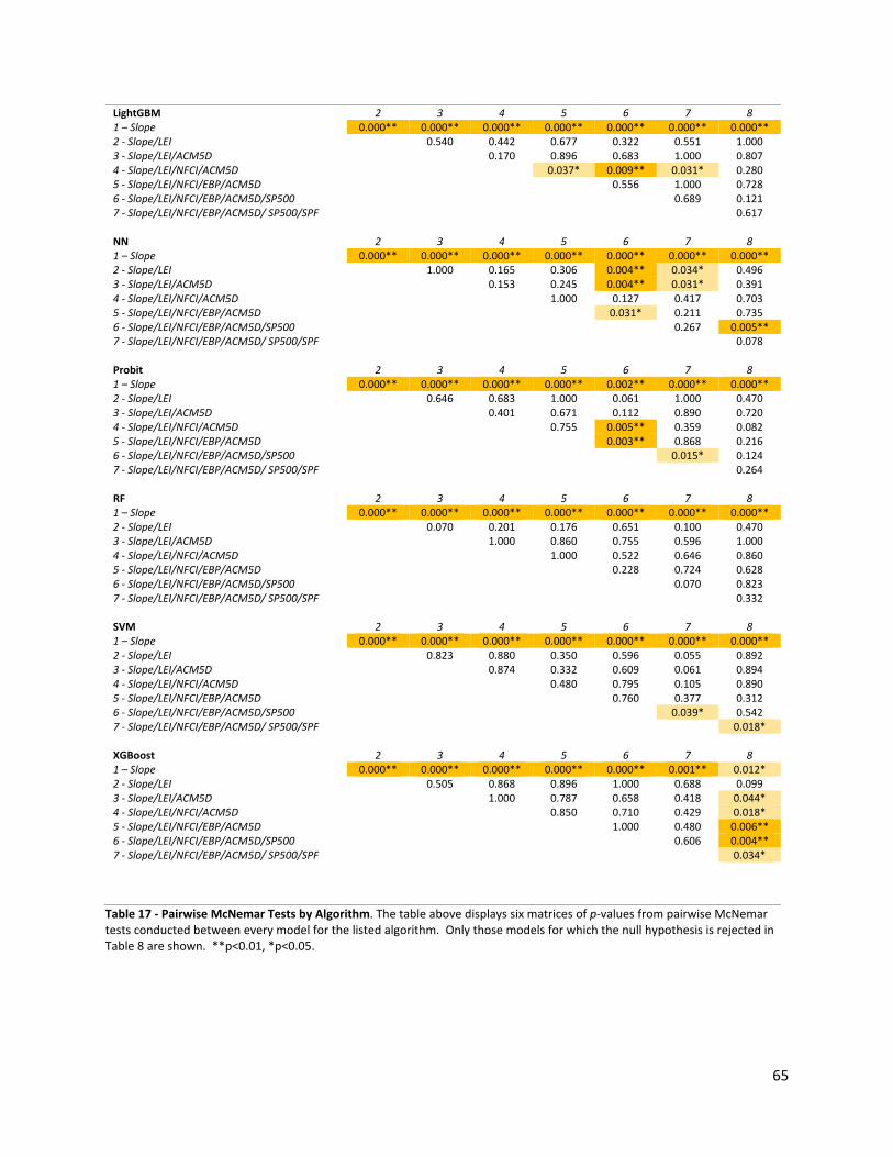
65

LightGBM 2 3 4 5 6 7 8 1 – Slope 0.000** 0.000** 0.000** 0.000** 0.000** 0.000** 0.000** 2 - Slope/LEI

0.540 0.442 0.677 0.322 0.551 1.000

3 - Slope/LEI/ACM5D

0.170 0.896 0.683 1.000 0.807 4 - Slope/LEI/NFCI/ACM5D

0.037* 0.009** 0.031* 0.280

5 - Slope/LEI/NFCI/EBP/ACM5D

0.556 1.000 0.728 6 - Slope/LEI/NFCI/EBP/ACM5D/SP500

0.689 0.121

7 - Slope/LEI/NFCI/EBP/ACM5D/ SP500/SPF

0.617

NN 2 3 4 5 6 7 8 1 – Slope 0.000** 0.000** 0.000** 0.000** 0.000** 0.000** 0.000** 2 - Slope/LEI

1.000 0.165 0.306 0.004** 0.034* 0.496

3 - Slope/LEI/ACM5D

0.153 0.245 0.004** 0.031* 0.391 4 - Slope/LEI/NFCI/ACM5D

1.000 0.127 0.417 0.703

5 - Slope/LEI/NFCI/EBP/ACM5D

0.031* 0.211 0.735 6 - Slope/LEI/NFCI/EBP/ACM5D/SP500

0.267 0.005**

7 - Slope/LEI/NFCI/EBP/ACM5D/ SP500/SPF

0.078 Probit 2 3 4 5 6 7 8 1 – Slope 0.000** 0.000** 0.000** 0.000** 0.002** 0.000** 0.000** 2 - Slope/LEI

0.646 0.683 1.000 0.061 1.000 0.470

3 - Slope/LEI/ACM5D

0.401 0.671 0.112 0.890 0.720 4 - Slope/LEI/NFCI/ACM5D

0.755 0.005** 0.359 0.082

5 - Slope/LEI/NFCI/EBP/ACM5D

0.003** 0.868 0.216 6 - Slope/LEI/NFCI/EBP/ACM5D/SP500

0.015* 0.124

7 - Slope/LEI/NFCI/EBP/ACM5D/ SP500/SPF

0.264

RF 2 3 4 5 6 7 8 1 – Slope 0.000** 0.000** 0.000** 0.000** 0.000** 0.000** 0.000** 2 - Slope/LEI

0.070 0.201 0.176 0.651 0.100 0.470

3 - Slope/LEI/ACM5D

1.000 0.860 0.755 0.596 1.000 4 - Slope/LEI/NFCI/ACM5D

1.000 0.522 0.646 0.860

5 - Slope/LEI/NFCI/EBP/ACM5D

0.228 0.724 0.628 6 - Slope/LEI/NFCI/EBP/ACM5D/SP500

0.070 0.823

7 - Slope/LEI/NFCI/EBP/ACM5D/ SP500/SPF

0.332

SVM 2 3 4 5 6 7 8 1 – Slope 0.000** 0.000** 0.000** 0.000** 0.000** 0.000** 0.000** 2 - Slope/LEI

0.823 0.880 0.350 0.596 0.055 0.892

3 - Slope/LEI/ACM5D

0.874 0.332 0.609 0.061 0.894 4 - Slope/LEI/NFCI/ACM5D

0.480 0.795 0.105 0.890

5 - Slope/LEI/NFCI/EBP/ACM5D

0.760 0.377 0.312 6 - Slope/LEI/NFCI/EBP/ACM5D/SP500

0.039* 0.542

7 - Slope/LEI/NFCI/EBP/ACM5D/ SP500/SPF

0.018*

XGBoost 2 3 4 5 6 7 8 1 – Slope 0.000** 0.000** 0.000** 0.000** 0.000** 0.001** 0.012* 2 - Slope/LEI 0.505 0.868 0.896 1.000 0.688 0.099 3 - Slope/LEI/ACM5D

1.000 0.787 0.658 0.418 0.044*

4 - Slope/LEI/NFCI/ACM5D

0.850 0.710 0.429 0.018* 5 - Slope/LEI/NFCI/EBP/ACM5D

1.000 0.480 0.006**

6 - Slope/LEI/NFCI/EBP/ACM5D/SP500

0.606 0.004** 7 - Slope/LEI/NFCI/EBP/ACM5D/ SP500/SPF

0.034*

Table 17 - Pairwise McNemar Tests by Algorithm. The table above displays six matrices of p-values from pairwise McNemar tests conducted between every model for the listed algorithm. Only those models for which the null hypothesis is rejected in Table 8 are shown. **p<0.01, *p<0.05.