Machining Accuracy Improvement Through Visual Control of an

Proceedings of 2011 NSF Engineering Research and Innovation Conference, Atlanta, Georgia Grant #0800507

Machining Accuracy Improvement Through Visual Control of an Active Display

Laine Mears, Ph.D., P.E.

Clemson University – International Center for Automotive Research

John Ziegert, Ph.D., P.E. Clemson University – International Center for Automotive Research

Abstract: The objective of this research is to formulate a physics-based predictive model relating achievable resolution of a new class of positioning system to a limited set of design parameters. The manufacturing lab at the Clemson University International Center for Automotive Research (CU-ICAR) has developed a new type of position sensing method using computer vision instead of optical position sensor. This new method is potentially to be implemented to a two dimensional motion control devices such as a CNC milling machine to provide better accuracy and high quality product, but is subject to fundamental control and image processing barriers. Thus, the goal of this project is to model the spatial resolution for this new class of position measurement system, and to explore the predictive efficacy of the model for spatial positioning. It is anticipated that sensing of a controllable array of pixel elements will allow high-precision motion control of simultaneous-axis positioning without need for error mapping and inversion. The prototype system is tested on a two-axis positioning stage for simultaneous axis closed-loop motion control.

1. Introduction: Computer Numerical Control (CNC) equipment is widely used in mass production to enable high-volume manufacturing with high accuracy. One of the determining factors for the resolution and accuracy of such equipment is the feedback sensing system used for axis positioning, typically linear or rotary encoders. However, in multi-axis motion systems, the feedback devices do not directly sense the position of the control point. Instead, the spatial position of the control point is estimated using the outputs of the position feedback sensors and a kinematic model of the machine. Inevitably, the kinematic model does not exactly describe the actual machine due to imperfect straightness of the axis guideways, non-squareness of their motion directions, and thermal variations with time, resulting in positioning errors. These errors have

traditionally been compensated using inverted error mapping applied to axis commands. This is a complex and expensive approach, and suffers from the fact that the error map is static and cannot compensate time-dependent effects. Alternative approaches suggest the use of other sensors, such as the system introduced in [1], which uses a 3D laser ball bar to measure the error of multi-axis machines. In [2], a new approach to multi-axis position feedback is presented, whereby a vision feedback system is implemented to directly sense the tool position rather than through the use of the traditional kinematic model. This system utilizes a ground-based camera trained on an active pixel display fixed to the stage being controlled. Target images on the active display are generated and then acquired by the camera, with the difference between the desired and actual target position on the camera image plane used to generate the error vector for drive commands (see Figure 1).

Figure 1: 2-Axis Stage Control through a Fixed Camera Acquiring Pixel Array Image from Position-Controlled Screen In this work, the achievable resolution of the described system is investigated when using a target image consisting of two intersecting curves displayed in pure

NSF GRANT # 0800507 NSF PROGRAM NAME: Manufacturing Construction Machines and Equipment


black/white form, i.e. no grayscale or color modulation of the target image is considered. The camera images this target, and analytic functions of the proper form are best-fit to the pixel data using a least-squares technique. The intersection of these functions is defined as the target location, which is then used to drive a positioning control scheme.

2. Background 2.1 Vision-Based Control: Manufacturing equipment must perform displacement measurements for feedback purposes in position control, typically in the micron and sometimes sub-micron range. In order to perform these measurements using vision acquisition devices imaging a target displayed on a flat panel display, sub-pixel resolution algorithms must be developed, since the typical pixel size of a camera or liquid crystal display screen is one or two orders of magnitude higher than the desired resolution. A brief review of vision-based motion control research is presented. Control of positioning through camera input has been accomplished in the past to a certain degree of accuracy. In Figure 2, the image capture and thresholding processing techniques capture a hand image, determine its outline, and quantify that information as an input to path planning for a motion system [3]. However, only lower accuracy positioning (in the order of 50µm) has been achieved with independent vision servoing.

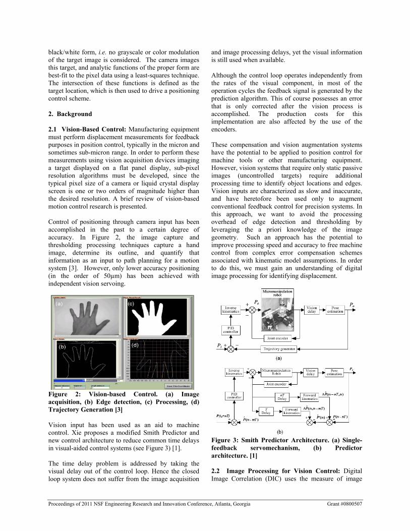
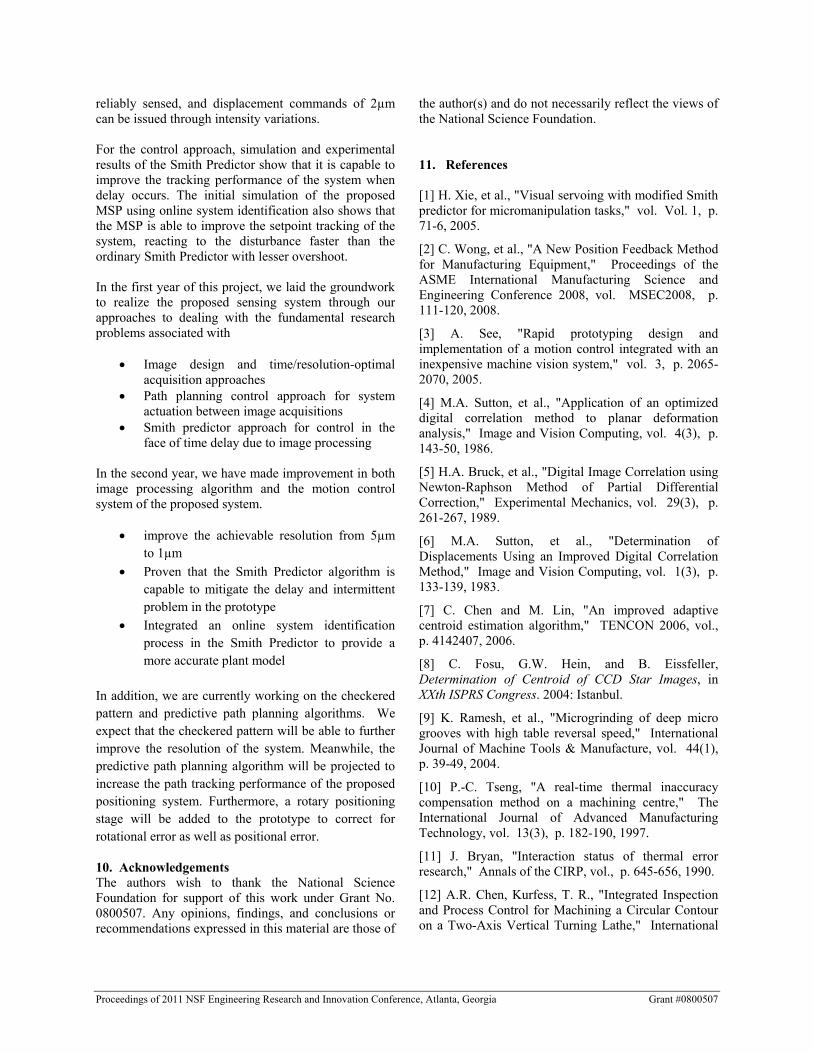
Figure 2: Vision-based Control. (a) Image acquisition, (b) Edge detection, (c) Processing, (d) Trajectory Generation [3] Vision input has been used as an aid to machine control. Xie proposes a modified Smith Predictor and new control architecture to reduce common time delays in visual-aided control systems (see Figure 3) [1]. The time delay problem is addressed by taking the visual delay out of the control loop. Hence the closed loop system does not suffer from the image acquisition

and image processing delays, yet the visual information is still used when available. Although the control loop operates independently from the rates of the visual component, in most of the operation cycles the feedback signal is generated by the prediction algorithm. This of course possesses an error that is only corrected after the vision process is accomplished. The production costs for this implementation are also affected by the use of the encoders. These compensation and vision augmentation systems have the potential to be applied to position control for machine tools or other manufacturing equipment. However, vision systems that require only static passive images (uncontrolled targets) require additional processing time to identify object locations and edges. Vision inputs are characterized as slow and inaccurate, and have heretofore been used only to augment conventional feedback control for precision systems. In this approach, we want to avoid the processing overhead of edge detection and thresholding by leveraging the a priori knowledge of the image geometry. Such an approach has the potential to improve processing speed and accuracy to free machine control from complex error compensation schemes associated with kinematic model assumptions. In order to do this, we must gain an understanding of digital image processing for identifying displacement.

Figure 3: Smith Predictor Architecture. (a) Single-feedback servomechanism, (b) Predictor architecture. [1] 2.2 Image Processing for Vision Control: Digital Image Correlation (DIC) uses the measure of image


correlation to optimize the parameters of transformation matrices between an acquired image and the known image geometry. Sutton initially described this approach in his establishment of a method to obtain full-field in-plane deformations of an object [4]. In his description, Sutton highlights the importance of pixel grayscale intensity in image digitization, and a transformation to a continuous representation form. DIC was successfully applied to large-scale planar deformation for measuring linear displacement using an efficient computation method [4]. However, in direct strain measurement using DIC, the method is found to have large variability in the computational result. Bruck enhanced the method using partial differential correction via a Newton-Raphson numerical approximation, and improved the ability to accurately measure strain [5]. In order to improve the system accuracy beyond the size of a discrete unit (pixel), forms of intensity-weighted distributions and bilinear interpolation have been implemented to discrete systems in order to represent the data in a continuous form. Sutton performed fundamental work with digital image correlation to represent image data in a continuous form which accounts for individual pixel intensity weighting [6]. This intensity-based representation allows for applications of mapping functions to transform the data for optimal correlation with the undeformed data set. Chen estimates the center of a discrete data set using an adaptive estimation algorithm, which improves the result of previous approaches to identification of the center of intensity of a noisy signal [7]. Such results are directly applicable to the centroid calculation on the image of imperfect screen pixel geometry. Finally, Fosu et al. determines the location of star images acquired by a discrete Charge-Coupled Device (CCD) microcircuit [8] using a point spread function and centroid calculation. Such results gained in the field of astronomy for accurately locating the positions of stars are readily applicable to determining the accurate location of manufacturing equipment position. 2.3 Machine Error: Based on the current configurations, one could argue that virtually all computer controlled multi-axis positioning systems operate under overall open-loop conditions. Although the individual axes of these machines do have positional feedback sensors and closed-loop control, the

actual coordinates of the tool control point (TCP) are not directly sensed. Instead, the axis positions, as measured by the sensors, are combined in a kinematic model of the machine to estimate the tool coordinates. For low precision applications, this approach is entirely adequate, but for high precision applications (e.g. coordinate measuring machines or semiconductor manufacturing equipment), the “as-built” machine does not exactly match the designed kinematic model, resulting in tool point positioning errors. The position error is the difference between the actual position and the desired position. For a typical 3-axis Cartesian machine, such as a milling machine, the tool coordinates are typically obtained directly from the readings of the X, Y, and Z axis position sensors. However, due to the imperfect construction of the guideways and the drive systems, as well as thermal expansion, and finite stiffness of the structure, these machines also possess 6 small positioning error components for each axis that are a function of the axis position: displacement errors along the 3 coordinate directions, rotational errors about the 3 coordinate axes, and 3 squareness errors associated to the relative alignments of the axes.

In general, there are three major sources of positioning error in machining equipment: geometric errors (including straightness, squareness and rotational error), temperature-induced errors caused by thermal expansion of the components, and force induced errors (e.g. cutting force during machining).

Thermal errors are typically the largest contributor to machine tool inaccuracies. Different heat sources, such as that coming from the machine drives or heat generated by the cutting process, affect the thermal state of the machine and the workpiece. The time-variant nature of these errors, the required assumptions about the temperature distributions between the discrete temperature sensors, and the difficulty in analyzing the heat flow in the machine structure, increase the difficulty and complexity of the corresponding correction algorithms [9-12].

2.4 Error Compensation: In order to increase the accuracy of machine tools, hardware improvement and software error compensation methods are desired [13]. Therefore, many studies and research have been carried out in investigating machine tool accuracy. A variety of error compensation solutions, such as error mapping, Homogeneous Transformation Matrices (HTM), rigid body kinematics and artificial intelligence control have been developed to address these issues. Some researchers even combine thermal and geometric models to predict the state of the machine under different conditions [14].


Although error compensation methods are able to correct positioning errors to a certain level of accuracy, this only happens after performing error mapping on the machine and after the correction signal is fed back through the control loop; this, of course, is time consuming and inefficient [13]. Even when using complex and detailed models, the individual error for the mathematical equation still has to be measured or predicted [15].

Additionally, other studies have used neural networks to address and compensate the thermal induced errors of a machine [16-20]. Although the induced error is indeed reduced, it takes several days to collect the data just to initiate the training process of the neural network [17].

A common pattern of most error compensation algorithms is the tedious task of creating geometric and thermal models and performing measurements required to parameterize these models. Additionally, the selection of calibration instruments, sensor placement, and complexity of thermal deformations represent major challenges in improving the accuracy of the system [21]. As more sensors are added to the machine, calibration and tuning become more complicated. 3. Direct Tool Position Sensing Most error compensation algorithms serve mainly as path correction sub-systems to the original CNC motion control system. These sub-systems supply corrected input signals, based on the error mapping algorithm. Figure 4(a) shows the nominal kinematic model of a position control machine, assuming perfect axis geometry, i.e. perfectly linear motion and orthogonal axes. However, the “as-built” machine guides look more like the dashed lines on the same figure. When one wishes to position the tool at some arbitrary spatial coordinate, the commands to the individual axes are obtained from the nominal (imperfect) kinematic model. The individual axis controllers then move the machine to this position as indicated by the axis scales. Thus, the imperfections in the nominal kinematic model lie outside the feedback loop, and therefore cannot be sensed nor corrected. Error compensation schemes simply modify the commanded positions to the axis controllers based on a pre-calibrated model of the machine. Figure 4 (b) shows the same machine with a multi-DOF spatial position sensor, used to directly monitor the position of the tool. When a position command is issued, the position error vector is the difference between the actual position, as measured by the multi-DOF sensor, and the commanded position. The vector

is then decomposed into individual axis position errors by the imperfect machine model. If the model errors are relatively small, the system will drive the tool towards the correct position. In this case, the imperfect machine model is inside the feedback loop, and its effects on the machine accuracy are reduced or eliminated.

(a)

(b)

Figure 4: (a) Conventional machine control system with independent axes b) Direct sensing coordinate system. In this research, direct 2-DOF sensing of the tool position is provided by visual feedback, from an actively controlled image on an LCD screen, using a digital camera. 4. Vision Approach The previous CMMI report in 2009 showed that the vision approach uses only two simple crossed lines as the dynamic target with a resolution of 5µm. This year, a newer vision approach has been further refined so that


the resolution of the system can be lower than 5µm, as presented in the following chapter. 4.1 Cross-Hair Dynamic Target: The first approach is to use the intersection of two perpendicular lines displayed on the LCD, i.e. a crosshair target. Previous tests have shown that for an 8-bit display, with pixel intensities varying from 0 (lowest, black) to 255 (highest: R, G or B), the optimal configuration is achieved by displaying a high-intensity target over black background (Figure 5 (a)). Aside from the crosshair target, four reference elements are displayed close to the intersection. These reference elements are spaced by known distances on the LCD and are used to estimate the magnification, f/Z, of a thin-lens perspective projection model, where f is the focal length and Z is the out-of-plane distance between the lens and the LCD. If the principal point PP on the CCD (Figure 5 (b)) is regarded as the reference, then an in-plane position error vector can be defined at any time t, with respect to this reference. As such, a target point C on the LCD would have an error vector e(t)=c on the CCD. This vector can be used as the control loop position error, where the controller’s goal is to bring the target to the reference position, i.e. PP.

(a) (b) Figure 5(a) Pixelated dynamic target on LCD with four Reference Elements, and (b) pinhole camera

model. 4.1.1 2-dimensional absolute positing through Newton Raphson interactive: The procedure for locating the target, once captured as a digital image though a CCD monochrome camera, is described in three steps: 1. Fine point location and definition of the line sets; 2. Constrained curve fitting through Newton-Raphson method; and 3. Estimation of pixel magnification using Reference Elements. 4.1.2 Fine Point Location and Definition of Sets: A fine point location on the CCD is achieved by calculating the intensity weighted center of mass or centroid around an intensity transition. An intensity

transition of interest is defined as a vertical or horizontal transition that starts in a black region, goes through a saturation point at 255 and finally goes back to a black region. For a discrete-valued function such as an image, I(x,y), where x varies in a discrete manner over a horizontal array of pixels e.g. 0 1∈ −[ , ]x m , and y is fixed to the current row under analysis e.g. y=j, the center of mass is

( )

( )

1

01

0

−

=−

=

=∑

∑,

,

,

m

i ii

C j m

ii

x I x jX

I x j (1)

The vertical centroid can be easily calculated by fixing x to a given column and letting y vary within a vertical neighborhood of interest. The target orientation, governed by θ, is measured with respect to the CCD X-axis and is used to determine the type of transitions present in the target image Figure 6. If 15θ ≤ ° then the image processing algorithm searches for both horizontal and vertical intensity transitions. Only horizontal transitions are analyzed, otherwise. The threshold value of 15° is selected based on trial and error tests using experimental data. Once the centroids are calculated they are separated in two sets later associated to two different lines.

Figure 6: Target orientation θ.

4.1.3 Constrained Curve Fitting: The location of the target is obtained by calculating the two lines that best fit the data collected in the previous step, and then analytically computing the intersection of these lines. The two data sets obtained from the previous step are denoted as DS1 and DS2 and are known to contain n1 and n2 data points, respectively. The best fit lines are constrained to be perpendicular with respect to each other. The previous statement is equivalent to finding ymodel, where

0 1 0 1

2 21

11 2

+ ∈ ∈⎧⎪= ⎨ − ∈ ∈⎪⎩

, , and

, andmodel

a a x a a R x DSy

a x a R x DSa

(2)

such that


( )

( )

2

0 1 2

22

0 1 21 2 1

1

= −

⎛ ⎞= − − + − +⎜ ⎟

⎝ ⎠

∑

∑ ∑

modely y( , , ) idata

i i i iDS DS

S a a a

y a a x y a xa

(3)

is minimized. The minimum is obtained by finding a0, a1, and a2 such that

0 10 0∂ ∂= =∂ ∂,S S

a a and

20∂ =∂

Sa .

From0 2

0 0∂ ∂= =∂ ∂,S Sa a

, respectively, the following

two equations result

( )0 2 1 11

1= −a v a v

n

(4)

2 2 12 1

1 1⎛ ⎞= +⎜ ⎟

⎝ ⎠a w w

n a (5)

where 2

1 2 3 41 1 1 1

= = = =∑ ∑ ∑ ∑, , ,i i i i iDS DS DS DS

v x v y v x y v x

and wi, i=1,..,4, is equivalent to vi but using DS2. The calculation of

10∂ =∂

Sa , knowing the results from (4)

and (5), yields a nonlinear equation of the form f(a1)=0, where f is assumed to have a continuous first derivative f’. This is

21 2 1

1 3 1 41 1

21 2 1

3 42 32 21 1

1 1 0

⎛ ⎞= − + − +⎜ ⎟

⎝ ⎠⎛ ⎞⎛ ⎞

− + − =⎜ ⎟⎜ ⎟⎝ ⎠ ⎝ ⎠

( )v v v

f a v a vn n

w w ww w

n na a

(6)

Equation (6) is solved using Newton-Raphson’s iterative method, which implies calculating

11 1

1

1 1 2+ = − =( ( ))

( ) ( ) , , ,...,'( ( ))

f a na n a n n k

f a n (7)

until

1 1 11 ε+ − ≤( ) ( ) ( )a n a n a n (8)

where a1(n) represents a constant value given to the variable a1, k is the total number of iterations, ɛ is an arbitrary threshold and the factor 1a n( ) in (8) is required in case of roots of very large or very small absolute value. Once a value for a1, satisfying (8), is found (4) and (5) can be calculated and (2) is fully defined. If the criterion diverges for a given target image, unconstrained curve fitting can still be conducted using the same datasets to obtained an alternative estimate.

4.1.4 Magnification: The magnification between the LCD- and CCD- pixels is obtained by determining the distance between the four Reference Elements on the CCD and comparing it with the real LCD spacing between these points. The locations of the Reference Elements on the target image are calculated with subpixel resolution using (1) over the areas containing these elements. 4.1.5 Command Issue-ing: One LCD pixel consists of three individual stripes (RGB). The intensity of a single LCD-pixel stripe is usually defined in an 8-bit scale. Color intensities on the LCD map to grayscale intensities on the CCD (also in the in an 8-bit scale for an 8-bit camera). Displacement commands are given by changing the intensity weighted centroid on the LCD target pixels, and thereby moving the target by increments in the order of microns. In practice, the camera cannot reliably distinguish between all possibly intensity states of the LCD display. Therefore, a thee-tone intensity basis, used to generate horizontal displacement commands, is selected and applies only to those pixels on the target vertical line:

{ }0 127 255= , ,XBI . Hence, a displacement basis can be

defined: ( ) { }0 00 32 58 49 00= ± ±. , . , .XBD I µm (Table 1).

From Figure 7it should be clear that the horizontal displacement basis only needs to cover a 0- to ±49µm range, starting from a reference stripe X0. For displacement bigger than |49|, a different reference stripe is selected. Table 1: Horizontal centroid change as a function of the intensities I(0) and I(1), corresponding to two adjacent stripes for LCD pixel size of 294x292µm

I(0) I(1) ΔXC (µm) 255 0 0.00 255 127 32.58 255 255 49.00

In order to command horizontal displacements of a fraction of the displacements provided by the basis, the LCD pixels on the target vertical line that lie within the camera FOV are divided in two sets; this is, a percentage of those pixels is set to exhibit a centroid in one location and the other percentage is set to exhibit a displaced centroid. For example, if a displacement command of 34µm was to be issued, 88% of the pixels in the vertical line would present a centroid at 32.58µm and 12% would present a centroid at 49.00µm. Notice that, 34≈0.88*32.58+0.12*49, with an error of less than one micron. For the case of vertical displacement commands a five-tone intensity basis is selected:


{ }0 80 130 180 255= , , , ,YBI A corresponding vertical

displacement basis is defined: ( ) { }0 00 58 26 82 40 101 00 122 00= ± ± ± ±. , . , . , . .Y

BD I µm. Due to the construction of the LCD pixels, vertical displacements are represented by intensity changes of whole pixels along the horizontal target line, as the individual stripes do not play a significant role for this matter. In general for any given orientation, θ, of the target with respect to the CCD plane, a 2-D displacement command ΔXCCD will require a displacement ΔXLCD of the target on the LCD screen. These two quantities are related through a rotation matrix Rθ, i.e. LCD θ CCDΔX = R ΔX .

Figure 7: One LCD pixel consisting of three stripes: R, G and B. 4.2 Checkered Pattern Identification: A second algorithm is proposed, where the object of interest on the display is embodied by four homogeneous grayscale-intensity areas, forming a checkered pattern (Figure 8 (a)). The main idea is to identify the location of the edges with high accuracy, correlate this data with two perpendicular lines and then, again, define the position of the target as the intersection of these lines. An important feature of the checkered pattern is the type of intensity transitions present in the image. This aspect is demonstrated when calculating the intensity gradient along the image X-axis (or Y-axis for vertical transitions), as shown in Figure 9. In order to estimate the position of the midpoint of an intensity impulse function, such as those in the cross-hairs target, an image processing algorithm based on edge-detection would have to deal with inaccuracies in the location of two edges (Figure 9 (a)). The checkered pattern presents potential advantages in this regard, as only one intensity transition happens around the pixels of interest (Figure 9 (b)).

(a) (b) Figure 8: (a) Theoretical active target represented by a checkered pattern and (b) corresponding 3D intensity plot. The checkered pattern method initiates with the calculation of the image gradient, for coarse-location of the edges. An edge is defined as a transition starting at a low-intensity pixel and ending at a high-intensity pixel (or the opposite of this: starting at a saturation point and ending at a low-intensity pixel), within a given pixel window. Fine point identification is performed by fitting a 1D Gaussian curve, to a horizontal or vertical array of pixels around an intensity peak in the gradient image, and taking the mean of the Gaussian curve as the fine location of the edge. This leads to the definition of two data sets, associated to two lines and containing the two-dimensional coordinates of the edges. The final step consists of determining the two perpendicular lines that best fit the two data sets.

(a)

(b)

Figure 9: (a) Intensity impulse function and corresponding gradient, plotted against image X-axis. (b) Intensity step function and corresponding gradient, plotted against image X-axis.

Step 1: Coarse point check through image gradient The first step consists in computing the image gradient. Although there are highly elaborated gradient filters, this step is intended for coarse point location only. A simple gradient operator, such as Prewitt, satisfies this initial criterion. Figure 10 shows a digital image of a checkered pattern, as captured through the camera. The 3D gradient graph in Figure 10 exhibits local maximums, not only around the target edges, but also in areas that map from high intensities pixels (white

Proceedings o

regions) oncamera is (black) gapwhen sensis also conminimumsintensity Ldistinguishgaps, witho

Figure 10(middle-leright) andright).

Figure 11rows of transition A valid edmaximum pixels (Y-athrough a hfinally goeshows thre

of 2011 NSF Engi

n the LCD. Thable to recog

ps that physicing high inten

nfirmed in the s are found inLCD pixels. A h between realout data losses

0: Snapshot oeft); correspond correspondin

: 2D gradienta checkered area of intere

ge is defined inin a row of pi

axis), that startshigh-intensity es back to a loee 2D gradien

neering Research

his phenomenongnize the smacally separate sity patterns o3D intensity p

n regions that robust algorith

l target edges .

of experimentnding 3D inteng 3D gradien

t curves for thpattern ima

est

n the gradient xels (X-axis) os at a low-intenpoint (not neceow-intensity re

nt curves, extra

and Innovation Co

n reveals that tall low intensthe LCD pixe

on the LCD. Thplot, where locmap from hi

hm is requiredand LCD pix

al target imaensity plot (tont plot (bottom

hree consecutiage, covering

image, as a locor in a column nsity pixel, goessarily 255) aegion. Figure acted from thr

onference, Atlanta

the sity els, his cal igh

d to els

age op-m-

ive

a

cal of

oes and 11 ree

consecusame tacontaintarget istated tfifth piincremthirteenintensitedge stpixel. Nrows 2 desiredcurve-fOn the does noThe loctwo arrtransititransiticonfuse Step 2: A fineGaussiaverticaldimensform

( ,f x A with x∈σx and is fittedThen, fcoordinwhere Gaussiaedge. Tthe posbut usivalue oThereforepresey va∈

curve tEdges care disrprocessedges htwo setlines.

a, Georgia

utive rows (Rarget image. Cn information mage. Based othat Row 2 preixel (pixels in ents of 1) andnth, dependingty threshold). tarting at the siNotice that the and 3 follow a

d as it can helpfitting process

contrary, the got comply withcal maximumsrows, in Figureons mapped ons can be thoed with target e

Fine edge lo

edge locationan curves thal edges, identifsional Gaussia

, , )xA Aμ σ =

[ , ], ,a b a b∈maximum amp

d to the rows ofor a valid hornates of the ed

x valid ed∈an curve that b

The same procesition of a vertiing pixels witof the x-coordinore, a vertical eented the alid edge anthat best fits close to the intregarded to avsing times. Ohave been idents, DSE1 and

Row 1, Row 2 learly, the pixeabout a hori

on the previousesents a valid this figure ared ending at thg the arbitraryLikewise, Rowixth pixel and ebehavior of th

a similar path; p improve thethat will be p

gradient curveh the requirems found in the ae 11, are clearly

from LCD ught of as noisedges for meas

ocus though Ga

n is achievedat best fit the fied in the grad

an function is

2

2( )

2x

x

x

Aeμ−

−σ

(9)

∈ , mean µplitude A. For f pixels containrizontal edge ldge on the imdge and µx best fits the daedure is followical edge with thin vertical ednate to the coledge located at

coordinates nd µy is the mthe data pointersection of th

void confusionnce the coord

ntified, these poDSE2 associa

Grant #0

and Row 3) els inside thesezontal edge os definition, it cedge, starting

e equally spache twelfth pixy value of thew 3 presents aending at the twhe gradient curthis characteri

e repeatability performed in se associated to

ment for a validarea enclosed by related to intpixel gaps.

se, and should surement purpo

aussian-curve f

d by calculatinvalid horizon

dient image. Thknown to hav

x, standard devhorizontal edgning the valid located at rowage plane are is the mean oata points with

wed when calcusub-pixel resoldges and fixinlumn under ant column j, wo

(j,µy), ean of the Ga

nts within the he checkered p

n and increase dinates of all oints are separaated to two dif

0800507

of the e rows on the can be at the

ed, by xel (or e low-a valid welfth rves in istic is of the

step 2. Row1

d edge. by the tensity These not be

oses.

fitting

ng the ntal or he one ve the

viation ges (9) edges.

w i, the (µx,i),

of the hin the ulating lution, ng the

nalysis. ould be

where aussian

edge. pattern image valid

ated in fferent

Proceedings o

Step 3: Cid

The locatiotwo perpenand DSE2analyticallyThis procecross-hairscalculated 5. ControIn the preapproach problem inthat the Sresponses w This year,prototype hmethod wenhanceme(MSP), to in the cont 5.1: Smithovercome the primarsystem mopotentiallyinstability. One of tmethods isform, an adpath in-bcontroller in Figure 1

In the outphysical sedead time the inner lo

of 2011 NSF Engi

Constrained cdentification

tanZθ−=

on of the targendicular lines t2 collected in y computing tedure is the ss target. The for a range of

ol Approach evious CMMIwas proposed

n the system. TSmith Predictowhen the delay

the Smith Phardware, and as implementeent termed thprovide a betteroller.

h Predictor: Tdelays in a cl

ry gains to incrore robust to thy leads to

the well knos the Smith Pdditional inneretween actuausing a genera

12[15].

Figure 12:

ter loop of thervo motor of or delay that coop, C(s) is th

neering Research

curve fitting

1

1

1a

− ⎛ ⎞⎜ ⎟⎝ ⎠ (10)

et is obtained bthat best fit the

the previousthe intersectioname as the derelative targe

[-π/2,π/2] throu

I report, the d to mitigate The simulationor is able toy occurs even w

Predictor was an online syst

ed to the Smhe Modified er estimation o

The most comosed loop systrease the damp

he delays[22]. sluggish pe

own dead-timPredictor (SP). r loop is includal feedback alized system

Smith Predic

he block diagrthe system, wh

caused by the vhe controller of

and Innovation Co

g and targ

by calculating te data sets DSE

s step, and thn of these lineveloped for tet orientation ugh (10)

Smith Predicthe time del

n results show provide robuwith high gains

deployed to tem identificatiith predictor, Smith Predic

of the model us

mmon method tem is by tuniping, making tHowever, this

erformance a

me compensati In this cont

ded to predict tsignals to tmodel as show

ctor

ram, G(s) is thich contains tvision system. f the plant, Geo

onference, Atlanta

get

the SE1 hen nes. the

is

tor lay

wed ust s.

the ion an tor sed

to ing the s is and

ion trol the the wn

the the In

o is

the delmodel. While during consistmodelsof y [23is show

SP

Once thcomparerror ecorrecttheoretieffectivthere arThe sysis constknown problem Thus, mhave bindustrymajor eare ovcontrolimprov 5.1.1: SPredictto be othe modlast yeathe acidentifi Figure simulatprocesssweep close es

a, Georgia

ay free plant m

the controller the dead tim

s of the both s will output an3]. The genera

wn in Eq. (11)

( )1 (

P sC s

=+

he actual feedbre with the de

ea to correct ths the actual pical analysis ovely mitigate dre still some flstem will havetant and the inin advance, in

m.

many Modifiedeen created foy. Simulationeffects on deadvercome, dynller are solved ved[24].

System Identitor, the plant mobtained. Thisdel order usingar’s report usinctual plant mication method

13 shows the ted signal of s based on a 0stimulus sign

stimation of th

model and Ge

waits for theme window, t

the delay freen emulated pa

al Smith Predic

0

( ))( ( )e e

C ss G s G−

back y is obtainsired setpoint he predicted epath of the syof the SP formdead time in c

flaws to be take steady state enitial conditionsn order for SP t

d Smith Predicor different den shows that d time of affecamic interactand overall ou

fication: In ormodel of the pros is first approg theoretical mng a second ordmodel was obd.

results of botthe offline sy

0.01-10Hz, 20Vnal. The simuhe actual measu

Grant #0

is the delayed

e actual feedbthe inner loope and delayed ath, v as a predctor transfer fu

( ))e s (1

ned, it is then uto output the

error, ee, whichystem. Althougm shows that closed loop coe into consider

error if the deas of the plant ato cure the dea

ctor (MSP) schead time systethe MSP has

cted systems: tions of delautput performa

rder to test the oposed system ached by estim

modeling, as shoder model. Thisbtained via s

th the measureystem identifiV peak-to-peaulated signal ured data.

0800507

d plant

ack, y p that servo

diction unction

11)

used to actual h also gh the it can ontrol, ration. d time are not ad time

hemes ems in s three delays

ays to ance is

Smith needs

mating own in s year, system

ed and ication ak sine shows


Figure 13: Measured (Dotted line) and simulated output (Solid line) waveforms

2

3 2

0.0000013445 0.0000047939 0.00000106079( )2.6119 2.23397 0.622284Model

z zG zz z z

+ +=

− + − (12)

Eq. (12) shows the plant model’s discrete transfer function generated by the offline system identification process. This model was used in the simulation and the hardware experiment of the Smith Predictor. The model is in the discrete to enable deployment into the micro-controller to validate the system performance. 5.2: Modified Smith Predictor (MSP): In order to update the plant model during the process, an online system identification process was integrated to the Smith Predictor as shown in Figure 14. Since the Smith Predictor relies heavily on the plant model to assist the system during the delay, online system identification process will be able to provide better estimation of the actual system. Similar to the ordinary Smith Predictor layout, a mathematical plant model, GModel(z) is used to serve as path predictor for the actual plant, GActual(z) during the delay period. Unlike the ordinary Smith Predictor, GModel(z) will be updated in real time rather than remaining static[9]. Although online system identification has been implemented in some industrial applications, it has typically been used to obtain better controller gains for the application[10]. However, online system identification is proposed to be integrated with the Smith Predictor to update the plant model, represented by the dotted line in Figure 14. As a result, disturbances such as thermal expansion and wear of machine components can also be taken into account and compensated automatically.

Figure 14: Modified Smith Predictor

Many online system identification methods have been developed to predict the plant model in real time: Least Mean Square, Normalized Least Mean Squares, Recursive Least Squares, and Kalman Filter. The Kalman Filter algorithm is chosen for this research to perform the online system identification because this algorithm will include quantification of the measurement noise and process noise when estimating the model. This is essential because the output of the plant model will be used as the actual path feedback during the delay period. In general, the Kalman Filter algorithm minimizes the mean square error between the actual plant position and the estimated model output position so that the predicted plant model has a closer approximation of the actual plant dynamics. 6: Path planning Path planning for this novel positioning system is also being developed uniquely due to the time delay and intermittent feedback within the system. 6.1 Predictive path planning: This algorithm uses a curve fitting algorithm not only to perform path planning but also to compensate the path error of the system. Step 1: Subdividing the desire path into fixed interval sections Before the machine starts, the a-priori position from initial position to the final position of the X-axis,

( )Apr 0 ft : tx of a desired design parts are known

ahead of time as shown in Figure 15. These points are typically generated by the Computer-Aided Manufacturing (CAM) software. In order to better represent the desired path accurately and improve the computational performance of the path planning algorithm, the desired path will be subdivided

into m section, ( )Apr m sectiontx in which the interval of


each m section, Tm is equal to 4τ, shown in Eq. (13). The selection of 4τ is because the curve fitting algorithm that will be discussed in later steps required 4 important position points: 2 previous actual data, a current estimated point and one future display point, to perform error compensation. At the same time, the system has a time delay, τ so each mentioned position points can only be obtained every τ ms. For instance, if τ is 500ms, then Tm is equal to 2000ms as illustrated in Figure 15.

4mT τ= (13)

Figure 15: A-priori position broken into sections

with fixed interval Step 2: Pixelation

Once each ( )Apr m sectiontx is generated, a set of pixel

coordinate for each section, ( ) m sectiontDisx will also

be generated using Eq. (14) so that these ( )tDisx can

be displayed on the digital display.

0 4, ,...,( ) ( ( ) )Dis apr of t t t

x t C x t xτ τ

= ⋅ + (14)

C is the scaling constant from axis displacement, mm to the digital display displacement unit. For example, if an LCD is used as the digital display, then the unit for C will be [mm/pixel]. xof is the offset value of the digital display to position the starting location of the axis at the zero coordinates pixel. Due to the image processing

time τ, ( )Dis tx will only be displayed or updated in the

intervals of time delay, as presented in Figure 17.

Figure 16: Pixelation- converting A-priori position to digital display position

Figure 17: Pixelation (Close up) Step 3: Obtain the previous actual positions

Once the machine is started, the obtained vision position at time t, ( )vx t is actually the actual position

at ( )t τ− , ( )vx t τ− .This is mainly due to the slow image processing time, τ causing the obtained position to be delayed by τ. Since the displayed locations of the previous points, ( )Disx t nτ− are known, where n is the number of previous display point, the previous position error, ( )ce t nτ− can be calculated using Eq.(15). For t=0, the previous errors will be assumed to be zero until the actual error of the system is obtained after τ.

1( ) ( ) ( ) nc Dis v ne t n x t n x t nτ τ τ =− = − − −

(15)

Figure 18 shows the algorithm of this step, where the green X represents ( )vx t nτ− , the blue X represents

( )Disx t and the red arrow represents ( )ce t nτ− .


Figure 18: Known previous vision positions with respect to their desired positions

Step 4: Estimate the current position Since the obtained position at time t, ( )vx t is actually

equal to ( )vx t τ− , the actual position at t will be

estimated, ˆ ( )vx t using extrapolation method. As an

initial phase, a second order predictor is proposed to predict the current position using the previous vision feedbacks. The second order predictor formulation is shown below:

2y at bt c= + +

21

2-2

-2 1

-2 1

1 22

^2

1

At 0,

At T,

At 2T, 4 2

4 2 3

4 3 2

2 2

n

n n

n n

n n n

n n n

n n n

n

t y c

t y aT bT y

t y aT bT y

y y bT y

y y ybT

y y yaT

y aT bT c

−

−

−

− −

+

= =

= − = − +

= − = − +

⇒ − = −

− +=

− + +=

∴ = + +

^

1 21 3 3n n nny y y y− −+ = − + (16)

Eq. (16) is the general formulation of the second order predictor, but in this case, ny is equal to ( )vx t τ− ,

1ny − is equal to ( 2 )vx t τ− , and 2ny − is equal to

( 3 )vx t τ− so Eq. (16) can be rewritten as Eq. (17)

ˆ ( ) 3 ( ) 3 ( 2 ) ( 3 )V V Dis V Dis V Disx t x t t x t t x t t= − − − + − (17) Then, the position error at time t, ˆ ( )ce t can also be predicted shown in Eq.(18)

( ) ( )cˆ ˆe t (t)- x t Dis Vx= (18)

Figure 19 shows the ˆ ( )vx t in the solid black star and

the ˆ ( )ve t in hollow arrow.

Figure 19: Previous errors and the estimated error

Step 5: Obtaining the correcting point Error compensation needs to be performed to drive the current position back to the desired position. This can be done by first obtaining the correcting points of the path, and then perform a curve fitting algorithm of these points to generate a new correction path from t to t+τ. Thus, the goal of this step is to obtain all the correcting points. As an initial phase of this new proposed algorithm, 4 correcting points: ( 2 )cx t τ− , ( )cx t τ− ,

ˆ ( )cx t and ( )Disx t τ+ ,are needed to generate the

correction path. Eq. 8 to 12 shows the formulation of each correcting point. ˆ ( )cx t has two options, either

( )x̂ tV or ( ) ( )cˆx̂ t e t V − which depend on the

correction options that will be discussed in the following step. Figure 20 shows the correcting points of the algorithm.

( 2 ) ( 2 ) ( 2 )c Dis cx t x t e tτ τ τ− = − − −

(19)

( ) ( ) ( )c Dis cx t x t e tτ τ τ− = − − −

(20)

( ) ( )( ) ( )

Smooth Correction c

c Instantaneous Correction

x̂ tˆ t

ˆx̂ t e t V

V

x⎡

= ⎢ −⎣ (21)


( ) ( )t+ t+c Disx xτ τ=

(22)

Figure 20: Obtaining the correcting points

Step 6: Generating correcting path

Once the correcting points are obtained, a set of interpolation setpoints denoted Virtual Intermittent

Setpoints (VIS), ( )VIS t : t x τ+⎡ ⎤⎣ ⎦ from ( )Disx t to

( )Disx t τ+ will be generated using curve fitting algorithm. As an initial phase, a cubic spline algorithm shown in Eq. (23) is used to perform the interpolation

of 4 selected correcting points, ( ) 2t tc tx τ

τ+−

ˆ( : ) [ ( 2 ), ( ), ( ), ( )]VIS c c c Disx t t spline x t x t x t x tτ τ τ τ+ = − − + (23)

The general formulation of spline interpolation algorithm used in the system is shown below:

2 21

2 1 2 2[ ]t i ii t i i

d x d xspline x Ax Bx C Ddt dt

ττ

+ +− += + + + (24)

Where

1

1

3 21

3 21

11 ( )( )61 ( )( )6

i

i i

i i

i i

t tAt t

B A

C A A t t

D B B t t

+

+

+

+

−=

−= −

= − −

= − −

Depending on the corection options: 1) Smooth correction or 2) Instantaneuos correction, the

( )VIS t : t x τ+⎡ ⎤⎣ ⎦will be generated differently. Figure

21 and Figure 22 shows the correction path of option 1 and 2, respectively.

Figure 21: Smooth correction path

Figure 22: Instantaneous correction path

Step 7: Repeat to Step 3 7. Prototype System For the proof of concept of the new approach, the independent axis position feedback sensors of an X-Y positioning stage are replaced by the combination of a digital camera and an active pixel array target. The testbed consists of an LCD monitor attached upside-down on top of a moving stage. A stationary camera is mounted below the stage as shown in Figure 1. Figure 23 shows the hardware configuration of the testbed. This configuration includes an NI 9014 CompactRIO real time controller with Field Programmable Gate Array (FPGA) and two NI 9505 H-Bridge Brushed DC Servo Drive Modules. Image acquisition and image processing are achieved using an IEEE-1394 camera connected to an NI Compact Vision System (CVS-1450). The communication between the different hardware components (Laptop-CompactRIO-CVS) is done through Ethernet.


Figure 23: Prototype system using servo-driven positioning of X-Y with camera capture of LCD

screen image. In this testbed, the desired motion trajectory of the stage is embodied as a time-varying sequence of images streamed on the LCD screen. The illuminated pixels on the display are captured in real time by the digital camera, and the stage motion control system attempts to keep the displayed image in the proper location with respect to the camera image plane. The result is an innovative online multi-DOF position feedback system. Hence, the design is more similar to a vision-based tracking controller than to a typical multi-axis machine. Additionally, because the sensor (camera) simultaneously monitors multiple degrees-of-freedom of the moving stage (X and Y displacements and Z rotation), the machine controller now becomes a MIMO (multi-input, multi-output) system as opposed to an assembly of SISO (single input-single output) systems. Therefore, the proposed camera-LCD sensing setup eliminates the reliance on the kinematic model, used to derive position targets for independent axes. This method also avoids traditional error compensation techniques, along with their associated cost and complexity. 8. Results Simulation, hardware prototyping, and data acquisition was performed to validate the proposed algorithms of the vision system, and motion controller. 8.1 Image Processing Algorithm: Experimental data is collected using bitmapped images, in order to minimize information losses due to image compression techniques. Multiple samples of the same static target presented standard deviations on the order of 0.2±0.1µm.

Figure 24: Zoom-in target image, showing a

horizontal displacement command.

Figure 25:11 horizontal displacement commands of

2µm are represented on the target image. The resulting best fit line has a slope of

1.8243µm/command and a regression coefficient of 0.9931.

Figure 26: 6 vertical displacement commands of 2µm are represented on the target image. The

resulting best fit line has a slope of 2.0304µm/command and a regression coefficient of

0.9962. 8.2 Smith Predictor: Simulation and hardware deployment of the Smith Predictor were performed. Before integrating the Smith Predictor with the vision sensor, the rotary encoder of the servo motor was used to emulate the vision sensor, by enforcing the time delay within the feedback loop from the encoder to the

y = 1.8243x ‐ 2.7296R² = 0.9931

‐5

0

5

10

15

20

0 5 10Vision Sensor (u

m)

Displacement Commands During 12 Time Steps

y = 2.0304x ‐ 2.1491R² = 0.9962

‐5

0

5

10

15

0 2 4 6Vision Sensor (u

m)

Displacement Commands During 7 Time Steps


motion controller. Two controllers were used in the simulation: 1) proportional-integral (PI) controller and 2) Smith Predictor using a PI controller, so that the results can be compared directly. Table 2 shows the gains used in both controllers. These gains were tuned to have less than 5% overshoot and less than 1% steady state error.

Table 2: Gains used in simulations

Smith Predictor PI Controller Delays P I P I 100ms 16 0.5 4.2 0.5 300ms 14 0.6 2 0.5

Figure 27: Simulation response with 100ms delay

Figure 28: Simulation response with 300ms delay

Figure 29: Simulation response with 100ms delay using same gains, P=16 and I=0.5

Table 3: Performance comparison for 100ms delay

Smith Predictor PI controller Rise Time 0.225s 0.741s Settling time 0.295s 1.352s

Figure 27 and Figure 28 illustrate the comparison of the Smith Predictor (Broken line) and PI controller (Dotted line) to track the setpoint (Solid Black) with 100ms and 300ms delays respectively. Based on the simulation results, it can be inferred that the Smith Predictor is

capable to improve the setpoint tracking performance of the system. The step response of the Smith Predictor shown in Figure 27 and Figure 28 has faster settling time and rise time than the ordinary PI controller, shown in Table 3. Due to the delay in the feedback, the P gain of the PI controller cannot be further increased to improve the step response performance while complying with the system requirement. The PI controller will have introduce oscillation if the P gain increased, as seen in Figure 29, where the P and I gain of the PI controller were configured to have the same values as the Smith Predictor Controller’s gains. In order to verify the performance, the Smith Predictor Controller was deployed to the microcontroller of the prototype and the actual responses are presented in Figure 30. During the hardware experiments, the Smith Predictor has 4.5% overshoot as seen in Figure 30, which complies with the system requirement, and has better performance than the PI controller.

Figure 30: Prototype response using square wave

reference Based on the preliminary experimental results of the simulation and the hardware experiments, it shows that the Smith Predictor controller (Broken line) has better tracking capability than the normal PI controller (Dotted line).

8.3 Modified Smith Predictor: To further improve the accuracy of the plant model used in the Smith Predictor, preliminary study and simulation of online system identification was also performed. Figure 31 shows the simulated feedback signal of the system. From 0 to 2.5 sec, no noise was injected but the Gaussian noise was injected into the feedback signal after 2.5 sec to emulate process or measured disturbance of the system. Figure 32 shows the predicted model output of the online system identification algorithm using the simulated output signal in Figure 31.


Figure 31: Actual signal with and without noise

Figure 32: Online system identification model’s

output Figure 33 shows the model denominator coefficients of the discrete plant model before and after the noise were injected. Before the noise was injected, all the coefficients’ values were constant, and were also close to the offline model’s coefficients generated by the offline system identification, shown in Eq.(12). When the Gaussian noise was injected to the output signal at 2.5 sec, the online system identification sensed the changes in the output signal and start predicting the plant model recursively with respect to the measured output. Figure 34and Figure 35 shows the close up look of the numerator and denominator coefficients of the discrete transfer function predicted by the online system identification when the noise was injected to the system.

Figure 33: Changes of the denominator’s coefficients

of the model when noise was injected at 2.5 sec

Figure 34: Changes of the denominator’s coefficients

of the model (scaled in time 3 to 6.5 sec)

Figure 35: Changes of the numerator’s coefficients

of the model when noise was injected at 2.5 sec

Figure 36: Simulation of the proposed MSP

Comparison between proposed MSP using online system identification to the ordinary Smith Predictor was also performed where a step input as the disturbance was injected to the feedback signal of the system shown in Figure 36. The simulation result shows that the MSP (Broken line) is capable to react faster than the SP (Solid line) when the disturbance (Broken Dotted line) was detected. In addition, the ordinary Smith Predictor has overshoot while recovering from the disturbance as can be seen at time 1.8s and 3.8s at the same time the ordinary Smith Predictor reacts 68ms slower than the MSP. Based on the simulation, it can be seen that the online system identification enhances the disturbance rejection performance of the system. 9. Conclusions and Continuing Work A 2-D position feedback method for real time control applications was presented. Experimental results demonstrate that resolutions on the order of 1µm can be


reliably sensed, and displacement commands of 2µm can be issued through intensity variations. For the control approach, simulation and experimental results of the Smith Predictor show that it is capable to improve the tracking performance of the system when delay occurs. The initial simulation of the proposed MSP using online system identification also shows that the MSP is able to improve the setpoint tracking of the system, reacting to the disturbance faster than the ordinary Smith Predictor with lesser overshoot. In the first year of this project, we laid the groundwork to realize the proposed sensing system through our approaches to dealing with the fundamental research problems associated with

• Image design and time/resolution-optimal acquisition approaches

• Path planning control approach for system actuation between image acquisitions

• Smith predictor approach for control in the face of time delay due to image processing

In the second year, we have made improvement in both image processing algorithm and the motion control system of the proposed system.

• improve the achievable resolution from 5µm to 1µm

• Proven that the Smith Predictor algorithm is capable to mitigate the delay and intermittent problem in the prototype

• Integrated an online system identification process in the Smith Predictor to provide a more accurate plant model

In addition, we are currently working on the checkered pattern and predictive path planning algorithms. We expect that the checkered pattern will be able to further improve the resolution of the system. Meanwhile, the predictive path planning algorithm will be projected to increase the path tracking performance of the proposed positioning system. Furthermore, a rotary positioning stage will be added to the prototype to correct for rotational error as well as positional error.

10. Acknowledgements The authors wish to thank the National Science Foundation for support of this work under Grant No. 0800507. Any opinions, findings, and conclusions or recommendations expressed in this material are those of

the author(s) and do not necessarily reflect the views of the National Science Foundation. 11. References [1] H. Xie, et al., "Visual servoing with modified Smith predictor for micromanipulation tasks," vol. Vol. 1, p. 71-6, 2005.

[2] C. Wong, et al., "A New Position Feedback Method for Manufacturing Equipment," Proceedings of the ASME International Manufacturing Science and Engineering Conference 2008, vol. MSEC2008, p. 111-120, 2008.

[3] A. See, "Rapid prototyping design and implementation of a motion control integrated with an inexpensive machine vision system," vol. 3, p. 2065-2070, 2005.

[4] M.A. Sutton, et al., "Application of an optimized digital correlation method to planar deformation analysis," Image and Vision Computing, vol. 4(3), p. 143-50, 1986.

[5] H.A. Bruck, et al., "Digital Image Correlation using Newton-Raphson Method of Partial Differential Correction," Experimental Mechanics, vol. 29(3), p. 261-267, 1989.

[6] M.A. Sutton, et al., "Determination of Displacements Using an Improved Digital Correlation Method," Image and Vision Computing, vol. 1(3), p. 133-139, 1983.

[7] C. Chen and M. Lin, "An improved adaptive centroid estimation algorithm," TENCON 2006, vol., p. 4142407, 2006.

[8] C. Fosu, G.W. Hein, and B. Eissfeller, Determination of Centroid of CCD Star Images, in XXth ISPRS Congress. 2004: Istanbul.

[9] K. Ramesh, et al., "Microgrinding of deep micro grooves with high table reversal speed," International Journal of Machine Tools & Manufacture, vol. 44(1), p. 39-49, 2004.

[10] P.-C. Tseng, "A real-time thermal inaccuracy compensation method on a machining centre," The International Journal of Advanced Manufacturing Technology, vol. 13(3), p. 182-190, 1997.

[11] J. Bryan, "Interaction status of thermal error research," Annals of the CIRP, vol., p. 645-656, 1990.

[12] A.R. Chen, Kurfess, T. R., "Integrated Inspection and Process Control for Machining a Circular Contour on a Two-Axis Vertical Turning Lathe," International


Journal of Manufacturing Research, vol. 1(1), p. 101-117, 2006.

[13] B.A. Woody, et al., "A technique for enhancing machine tool accuracy by transferring the metrology reference from the machine tool to the workpiece," Journal of Manufacturing Science and Engineering, Transactions of the ASME, vol. 129(3), p. 636-643, 2007.

[14] R.J. Hocken, Trumper, D. L. , Wang, C., "Dynamics and Control of the UNCC/MIT Sub-Atomic Measuring Machine," CIRP Annals - Manufacturing Technology, vol. 50(1), p. 373-376, 2001.

[15] J. Mou and M.A. Donmez, "Integrated inspection system for improved machine performance," vol. 2063, p. 22-31, 1993.

[16] J.-S. Chen, "Computer-aided accuracy enhancement for multi-axis CNC machine tool," International Journal of Machine Tools & Manufacture, vol. 35(4), p. 593-605, 1995.

[17] N. Srinivasa and J.C. Ziegert, "Automated measurement and compensation of thermally induced error maps in machine tools," Precision Engineering, vol. 19(2-3), p. 112-132, 1996.

[18] J. Mou, Domez, M. A., and Cetinkunt, S., An Adaptive Error Correction Method Using Feature-Based Analysis Techniques for Machine Performance Improvement, Part 1: Theory Derivation,” in American Society for Mechanical Engineers Winter Annual Meeting Symposium of Intelligent Machine Tool System. 1994: Chicago. p. 584-590.

[19] C.D.Z. Mize, John C., "Durability evaluation of software error correction on a machining center," International Journal of Machine Tools and Manufacture, vol. 40(10), p. 1527-1534, 2000.

[20] C.D. Mize and J.C. Ziegert, "Neural network thermal error compensation of a machining center," Precision Engineering, vol. 24(4), p. 338-346, 2000.

[21] J. Ni, "CNC machine accuracy enhancement through real time error compensation," Transactions of the ASME. Journal of Manufacturing Science and Engineering, vol. 119(4B), p. 717-25, 1997.

[22] T.P. Sim, G.S. Hong, and K.B. Lim, "Multirate predictor control scheme for visual servo control," IEE Proceedings: Control Theory and Applications, vol. 149(2), p. 117-124, 2002.

[23] Z. Palmor, Time-delay compensation - Smith predictor and its modifications. 1996, CRC Press. p. 224-237.

[24] C. Brown, "Gaze controls with interactions and delays," IEEE Transactions on Systems, Man and Cybernetics, vol. 20(2), p. 518-527, 1990.

[25] R. Dunia and J. Gutierrez, Graphical MPC For Fast Dynamic Systems, in Manufacturing Science and Engineering Conference 2008: Evanston, Illinois, USA.

[26] I. National, Control design user manual 2008.

[27] Edmund Optics, "Electronic Imaging Resource Guide," vol. (13Oct2008), Available from: http://www.edmundoptics.com/TechSupport/DisplayArticle.cfm?articleid=286, 2008.

Documents

Machining Accuracy Improvement Through Visual Control of an