Macro Economics Introuction

8/14/2019 Macro Economics Introuction

http://slidepdf.com/reader/full/macro-economics-introuction 1/62

ECOS2002

Intermediate Macroeconomics

Lecturer: Matthew Smith

Topic 2

National Accounting, the KeynesianIncome-Expenditure Model and FiscalPolicy

School of EconomicsFaculty of Arts and Social Science



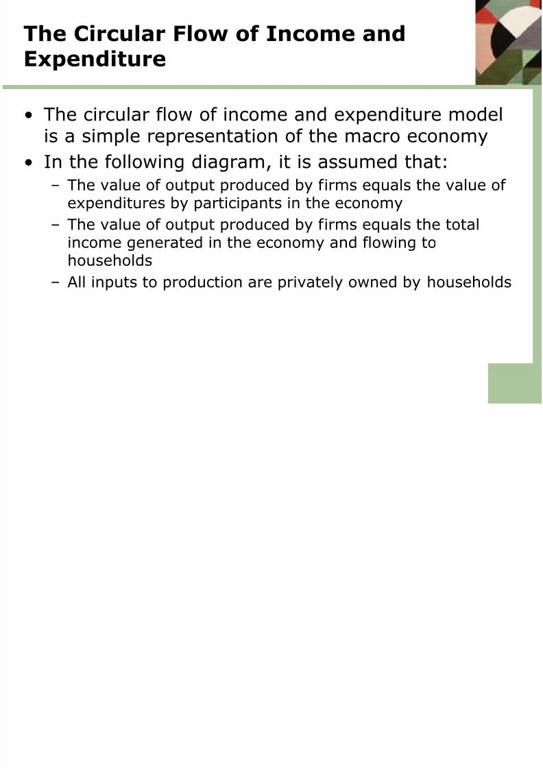
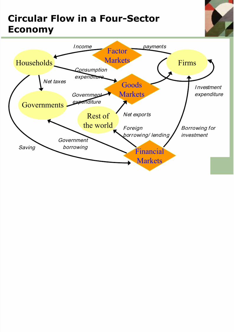
The Circular Flow of Income andExpenditure

• The circular flow of income and expenditure modelis a simple representation of the macro economy

• In the following diagram, it is assumed that:

– The value of output produced by firms equals the value ofexpenditures by participants in the economy

– The value of output produced by firms equals the totalincome generated in the economy and flowing tohouseholds

– All inputs to production are privately owned by households



Goods

Markets

Financial

Markets

Circular Flow in a Four-SectorEconomy

Governments

Rest of

the world

Government

borrowing

Foreign

borrowing/ lending

Household

s

Net taxes

Consumption

expenditure

Net expor ts

Borrowing for

investment

Government

expenditure

I nvestment

expenditure

Saving

Factor

Markets Firms

I ncome payments

Households



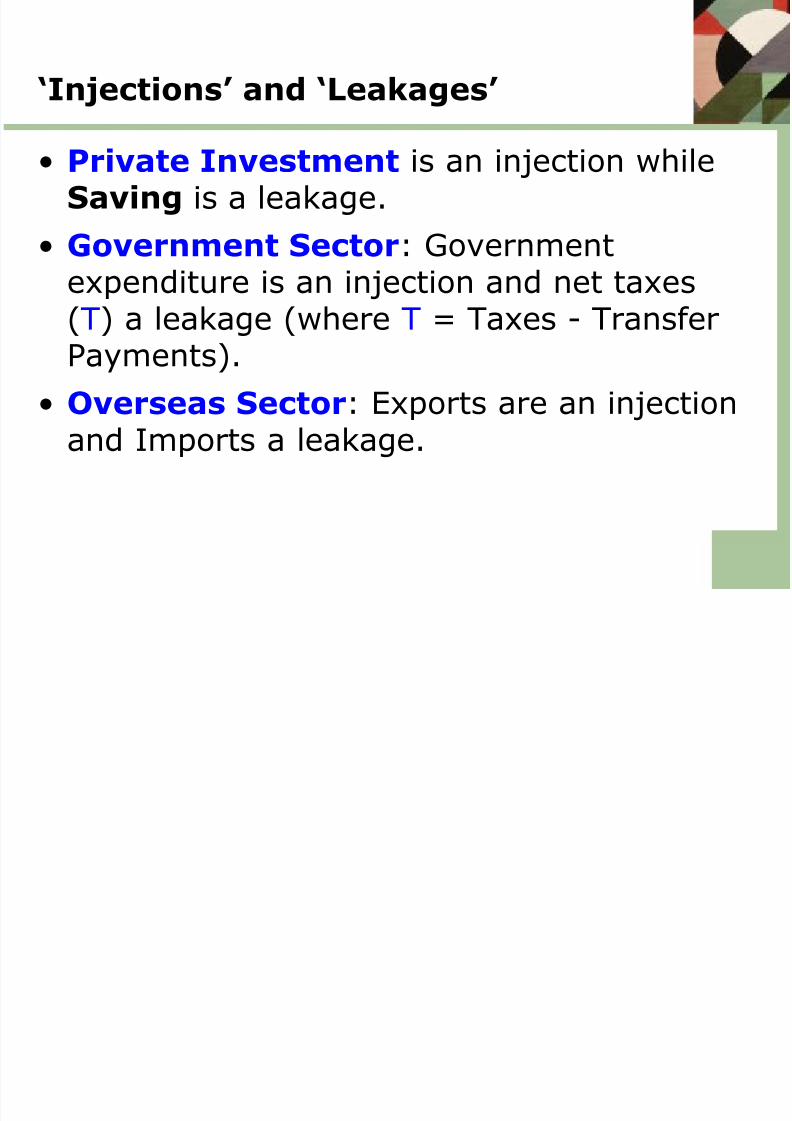
‘Injections’ and ‘Leakages’

• Private Investment is an injection whileSaving is a leakage.

• Government Sector: Government

expenditure is an injection and net taxes(T) a leakage (where T = Taxes - TransferPayments).

• Overseas Sector: Exports are an injectionand Imports a leakage.



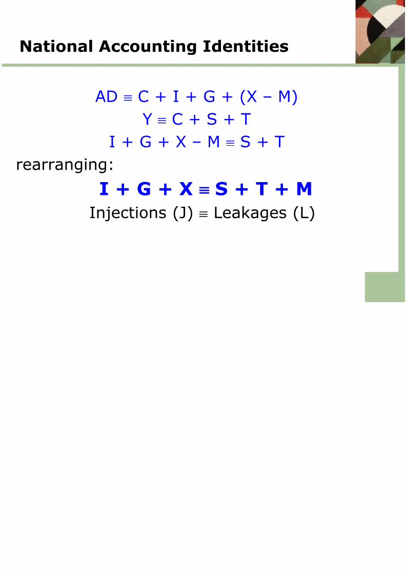
National Accounting Identities

AD C + I + G + (X – M)

Y C + S + T

I + G + X – M S + Trearranging:

I + G + X S + T + M

Injections (J) Leakages (L)



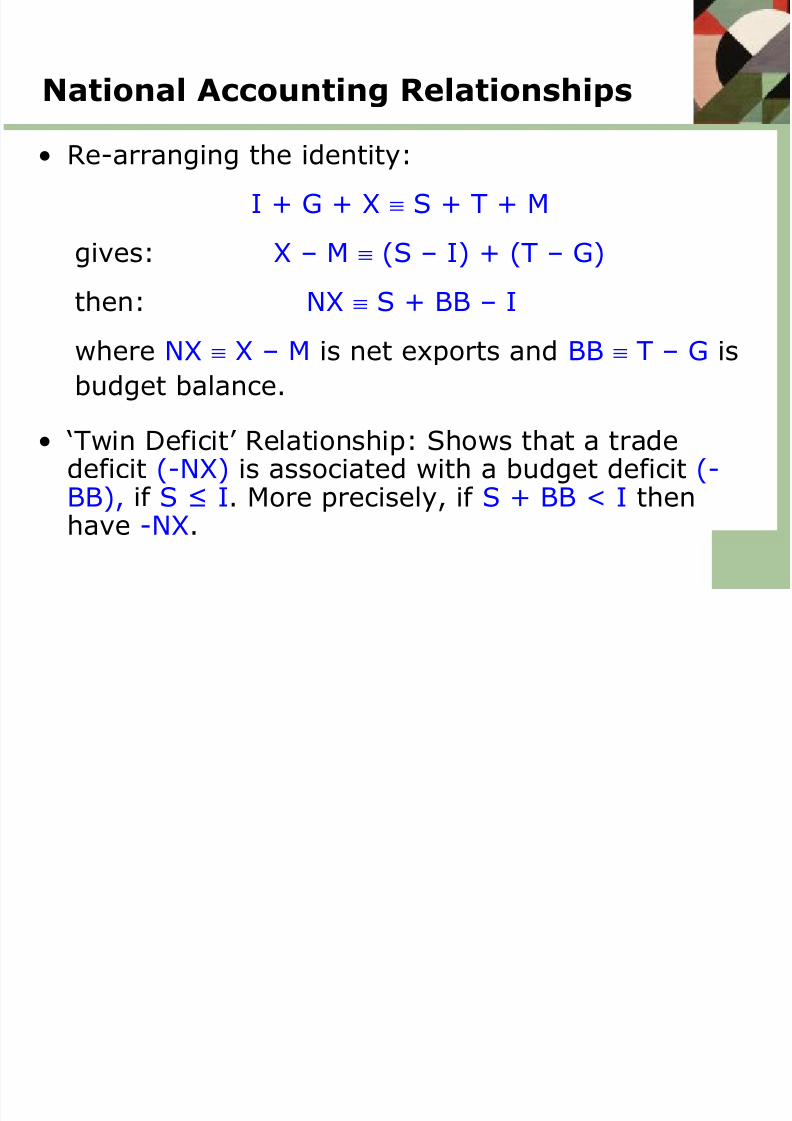
National Accounting Relationships

• Re-arranging the identity:

I + G + X S + T + M

gives: X – M (S – I) + (T – G)

then: NX S + BB – I

where NX X – M is net exports and BB T – G is

budget balance.

• ‘Twin Deficit’ Relationship: Shows that a tradedeficit (-NX) is associated with a budget deficit (-BB), if S ≤ I. More precisely, if S + BB < I thenhave -NX.



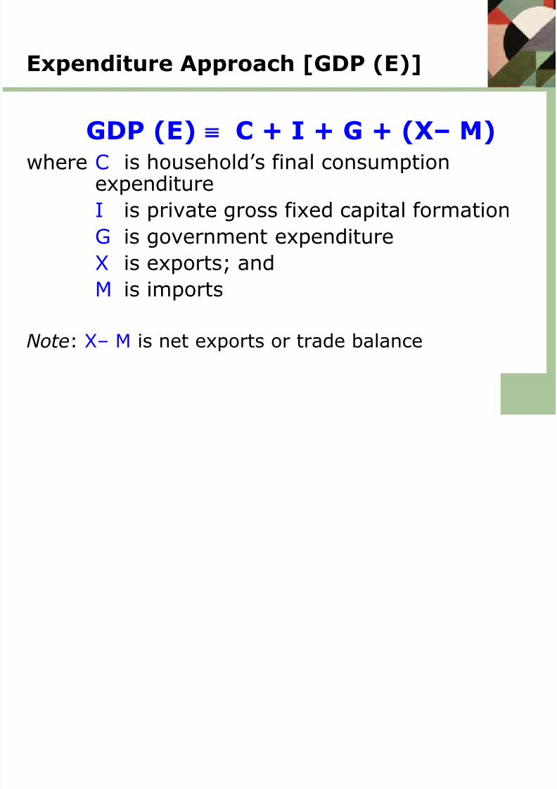
Expenditure Approach [GDP (E)]

GDP (E) C + I + G + (X– M) where C is household’s final consumption

expenditureI is private gross fixed capital formation

G is government expenditure

X is exports; and

M is imports

Note: X– M is net exports or trade balance



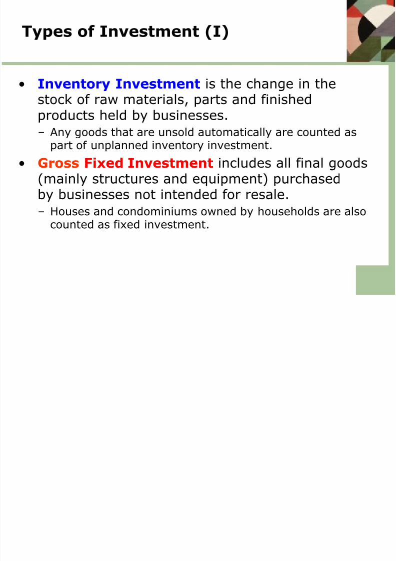
Types of Investment (I)

• Inventory Investment is the change in thestock of raw materials, parts and finishedproducts held by businesses.

– Any goods that are unsold automatically are counted aspart of unplanned inventory investment.

• Gross Fixed Investment includes all final goods(mainly structures and equipment) purchasedby businesses not intended for resale.

– Houses and condominiums owned by households are alsocounted as fixed investment.



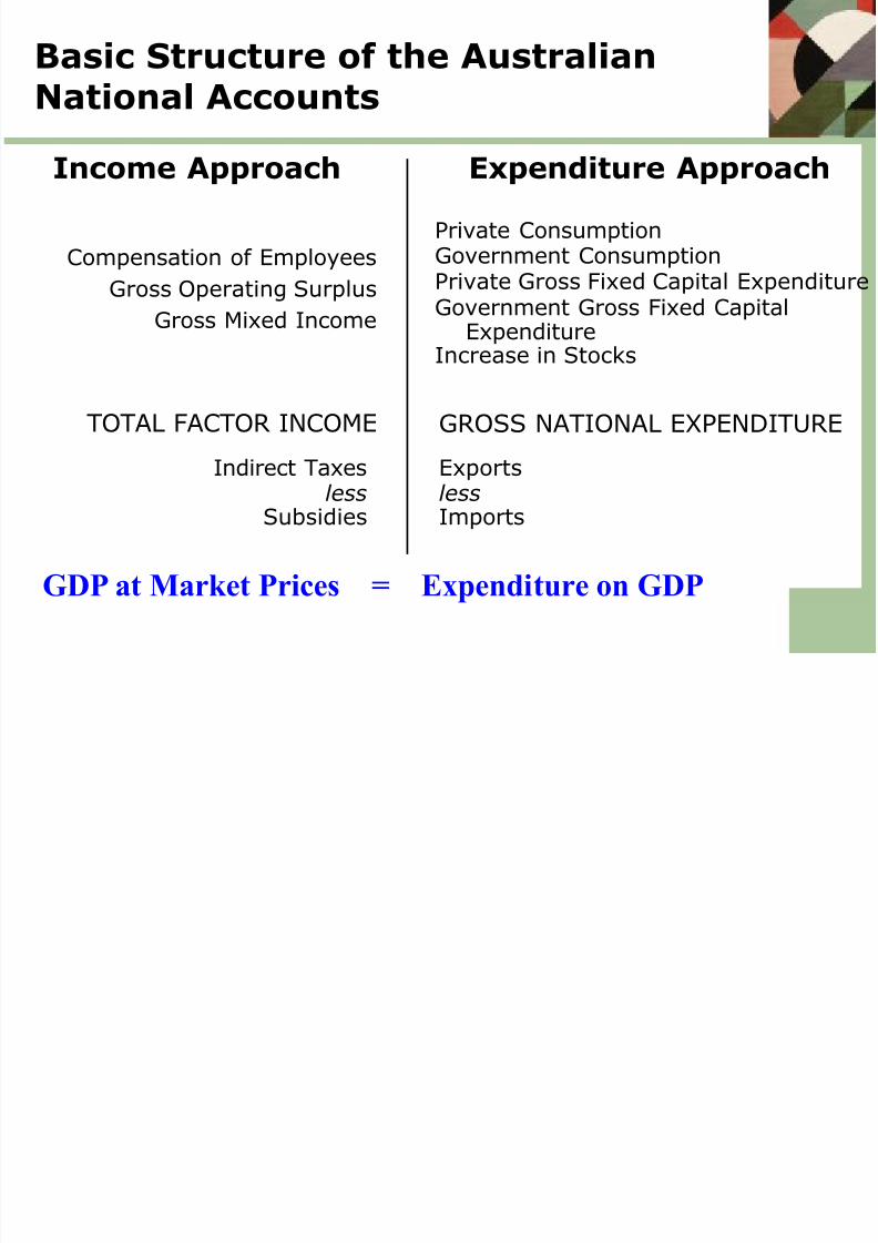
Basic Structure of the AustralianNational Accounts

Income Approach Expenditure Approach

Compensation of Employees

Gross Operating Surplus

Gross Mixed Income

Private ConsumptionGovernment ConsumptionPrivate Gross Fixed Capital Expenditure

Government Gross Fixed CapitalExpenditure

Increase in Stocks

GDP at Market Prices = Expenditure on GDP

TOTAL FACTOR INCOME GROSS NATIONAL EXPENDITURE

Indirect Taxesless

Subsidies

ExportslessImports



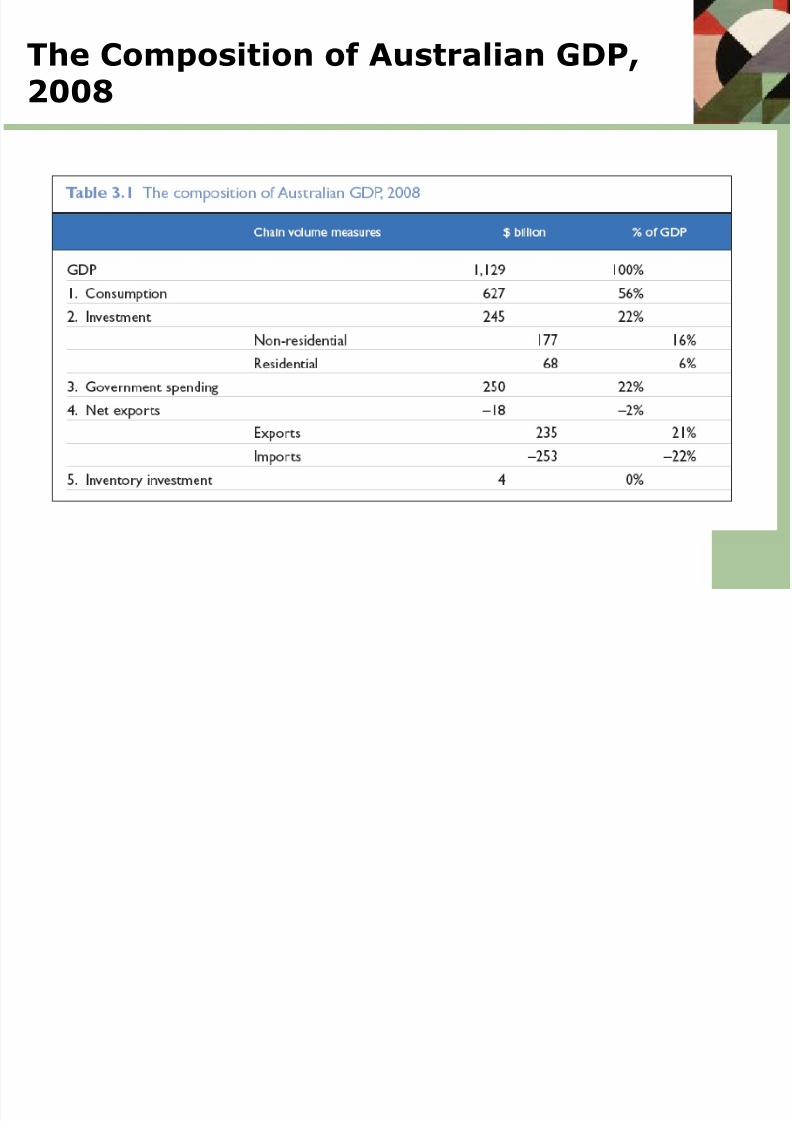
The Composition of Australian GDP,2008



Measuring Unemployment

• The unemployed are those without who either are ontemporary layoff or have taken specific action to look for work

• The total labor force is total of the civilian employed, thearmed forces and the unemployed

• The actual unemployment rate (U) is defined below:

• The ABS Labour Force Survey produces employment andunemployment data, based on a monthly survey of 42000matched households.



Macroeconomic Equilibrium

From the exposition of national accounting, it isevident that real aggregate output is equal to realnational income and is equal to real aggregate

expenditure.

This is a national accounting identity:

Y AE (ex poste)




• In a simple ‘two-sector’ model with only ‘firms’

and ‘households’ it follows that:

C + S C + I (ex poste)

S I (ex poste)

• This states that actual levels of investment and

saving must be equal when actual income and

aggregate expenditure are equal. This identity

follows by definition.




• Not the same thing as a national accountingidentity

• A position of stability in which economic forcesare tending to push the economy

• A ‘centre of gravity’ in which the economicsystem is tending toward or oscillating around

• Not a position at which the actual economy canbe in – no theory can provide an explanation ofthe of the actual economy given its complexity.




• Macroeconomic equilibrium is conceived to be aposition at which the plans of agents are realisedor are compatible.

• In our simple two-sector model, equilibriumoutput will be characterised by equality betweenplanned investment and planned saving.

• In three- and four-sector models macroeconomicequilibrium is characterised by equality betweeninjections and leakages (see below).



Equilibrium versus Disequilibrium

Equilibrium: Ip = Sp (ex ante)

• Investment decisions undertaken by firms

• Saving decisions undertaken by households.

• These decisions are therefore undertaken bydifferent groups of economic agents withdifferent motives.

• For this reason saving plans and investmentplans will not automatically match.



Equilibrium versus Disequilibrium

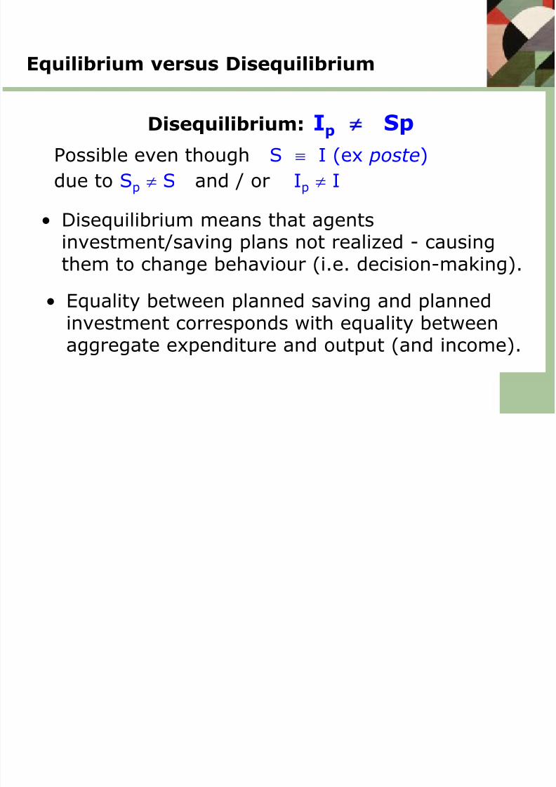
Disequilibrium: Ip Sp

Possible even though S I (ex poste)

due to Sp S and / or Ip I

• Disequilibrium means that agentsinvestment/saving plans not realized - causingthem to change behaviour (i.e. decision-making).

• Equality between planned saving and plannedinvestment corresponds with equality betweenaggregate expenditure and output (and income).




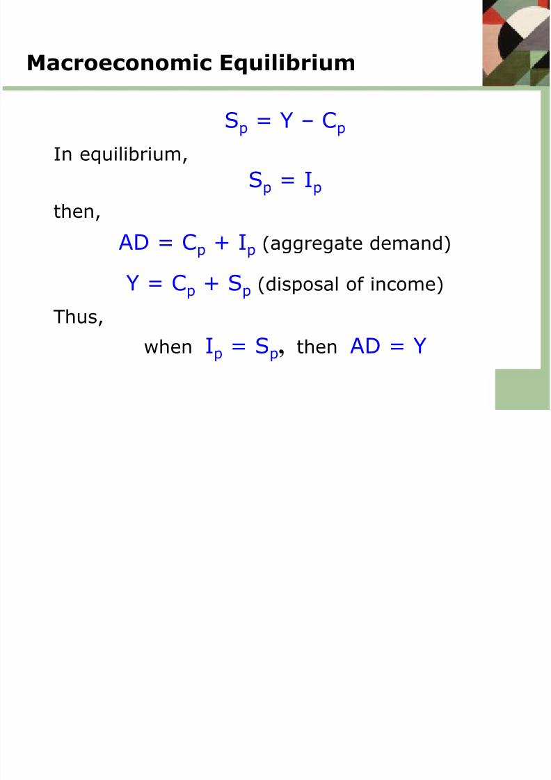
Sp = Y – Cp

In equilibrium,

Sp

= Ip

then,

AD = Cp + Ip (aggregate demand)

Y = Cp + Sp (disposal of income)Thus,

when Ip = Sp, then AD = Y



Macroeconomic Equilibrium versusDisequilibrium

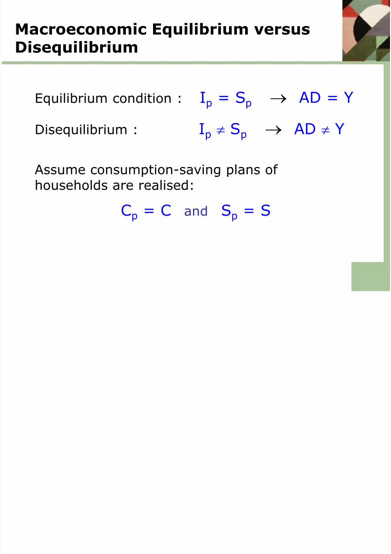
Equilibrium condition : Ip = Sp AD = Y

Disequilibrium :

Ip S

p AD Y

Assume consumption-saving plans ofhouseholds are realised:

Cp = C and Sp = S



Macroeconomic Equilibrium versusDisequilibrium

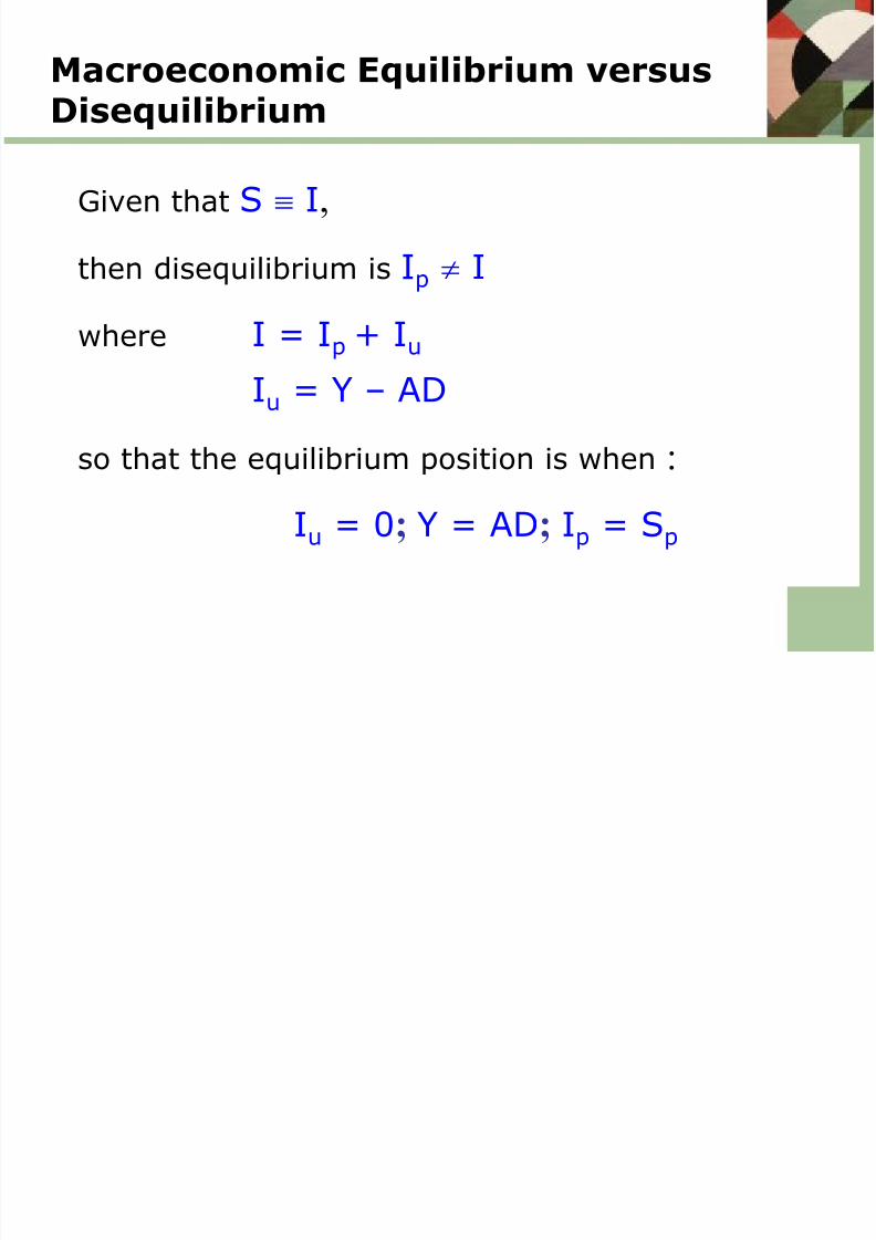
Given that S I,

then disequilibrium is Ip I

where I = Ip + Iu

Iu = Y – AD

so that the equilibrium position is when :

Iu = 0; Y = AD; Ip = Sp



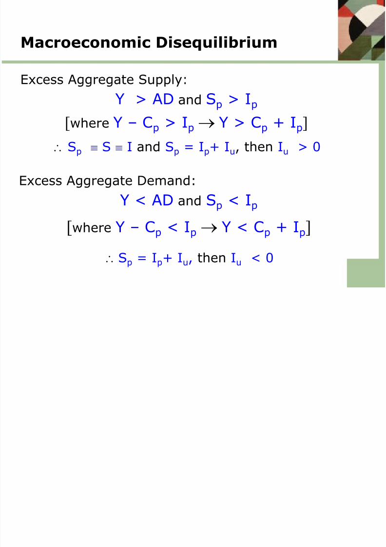
Macroeconomic Disequilibrium

Excess Aggregate Supply:

Y > AD and Sp > Ip

[where Y – Cp > Ip Y > Cp + Ip]

Sp S I and Sp = Ip+ Iu, then Iu > 0

Excess Aggregate Demand:

Y < AD and Sp < Ip [where Y – Cp < Ip Y < Cp + Ip]

Sp = Ip+ Iu, then Iu < 0



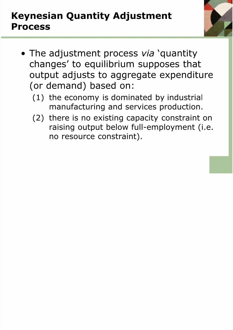
Keynesian Quantity AdjustmentProcess

• The adjustment process via ‘quantitychanges’ to equilibrium supposes thatoutput adjusts to aggregate expenditure

(or demand) based on:

(1) the economy is dominated by industrialmanufacturing and services production.

(2) there is no existing capacity constraint onraising output below full-employment (i.e.no resource constraint).



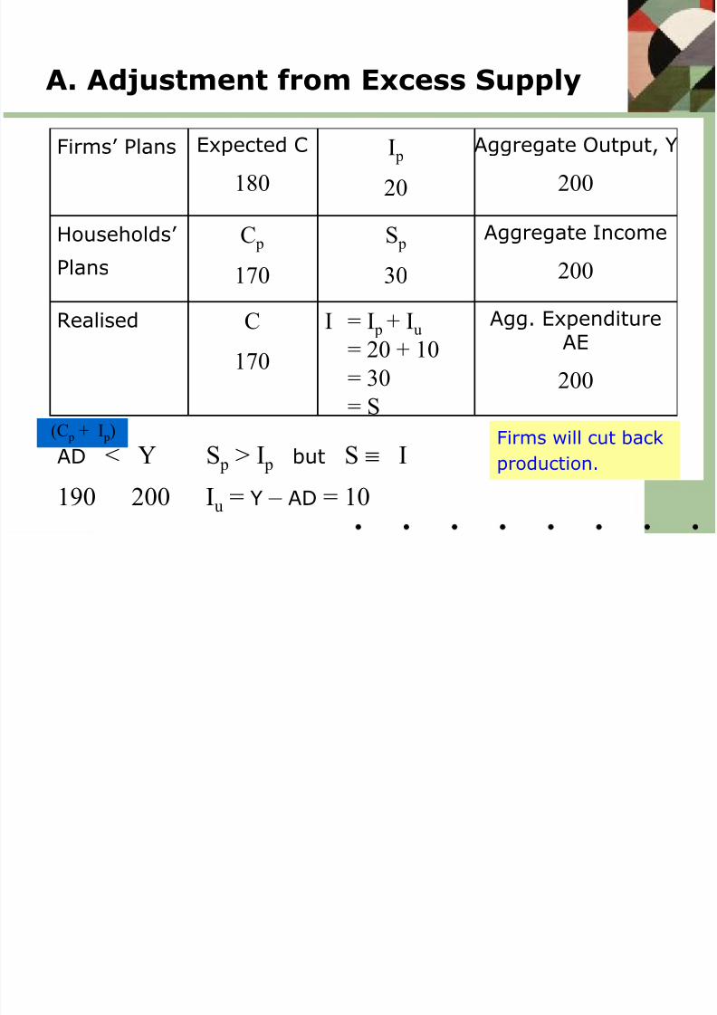
A. Adjustment from Excess Supply

Firms’ Plans Expected C

180

I p

20

Aggregate Output, Y

200

Households’

Plans

C p

170

S p

30

Aggregate Income

200

Realised C

170

I = I p + Iu

= 20 + 10

= 30= S

Agg. ExpenditureAE

200

AD < Y S p > I p but S I

190 200 Iu = Y –

AD = 10

Firms will cut back

production.

(C p + I p)



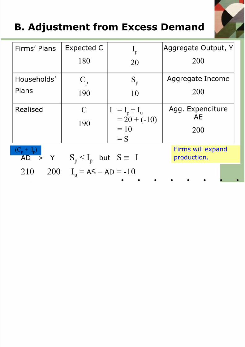
B. Adjustment from Excess Demand

Firms’ Plans Expected C

180

I p

20

Aggregate Output, Y

200

Households’

Plans

C p

190

S p

10

Aggregate Income

200

Realised C

190

I = I p + Iu

= 20 + (-10)

= 10= S

Agg. ExpenditureAE

200

AD > Y S p < I p but S I

210 200 Iu = AS – AD = -10

Firms will expand

production.(C p + I p)



• Aggregate demand depends on planned investment,

Ip, consumption, Cp, and government spending, G:

AD = Cp

+ Ip

+ G

Y = Cp + Sp + T

where T is net taxes.

• Need to explain Cp , Ip , G, T and Sp and show how

[Ip + G] brought into equality with [Sp + T],

corresponding to, AD = Y. .

Keynesian Three-Sector Model



Consumption Function

Cp = f (Y) (1)

A simple linear consumption function is:

Cp = Co + c .Y (2)

Co is exogenous consumption (that partdependent on factors other than current income

such as interest rates, wealth effects etc.);c is the marginal propensity to consume out ofincome (where c = ∆C/∆Y, 0<c< 1).



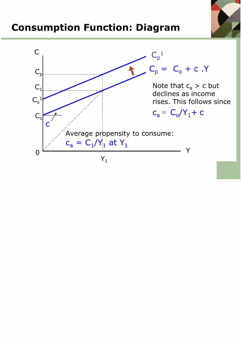
Consumption Function: Diagram

Average propensity to consume: ca = C1 /Y1 at Y1

C1

Co

Y1 0 Y

Cp

Co1

Cp1

c

Note that ca > c butdeclines as incomerises. This follows since

ca = Co /Y1+ c

Cp = Co + c .Y

C



Net Taxes

Disposable income, YD, is equal to aggregate income generatedin production, plus transfer payments (TP) less taxes (TA):

YD = Y + TP – TA (3)

No distinction is made here between direct taxation (levied on

income) and indirect taxation (levied on expenditures).

Given that tax revenue will be greater than transfer paymentsthis expression can be simplified to:

YD = Y – T (4)

where T = TA – TP and is net taxes. To begin we assume

net taxes are exogenously determined by government:

T = To (5)



Consumption Function withGovernment Sector

The consumption function is now specified as:

Cp = Co + c . (Y – To) (6)

Expanding (6):Cp = Co + c. Y – c.To (7)

•It is assumed that consumption demand is a stablefunction of aggregate household disposable income.

•The function makes no allowance for the effect ofchanges in taxation and transfer payments on thedistribution of aggregate disposable income.

•Effect of distributional changes likely to operate via

the value of c of society.



Saving Function

Planned saving is a positive function of aggregate(disposable) income:

Sp = f (Y) (8)

It is freely disposable income of the private sectornot devoted to consumption:

Sp = Y Cp (9)

Substituting (7) into (9) we can derive the following

saving function:

Sp = Y [Co + c.Y – c.To] (10)then:

Sp = -Co + c.To + (1c).Y (11)



Saving Function

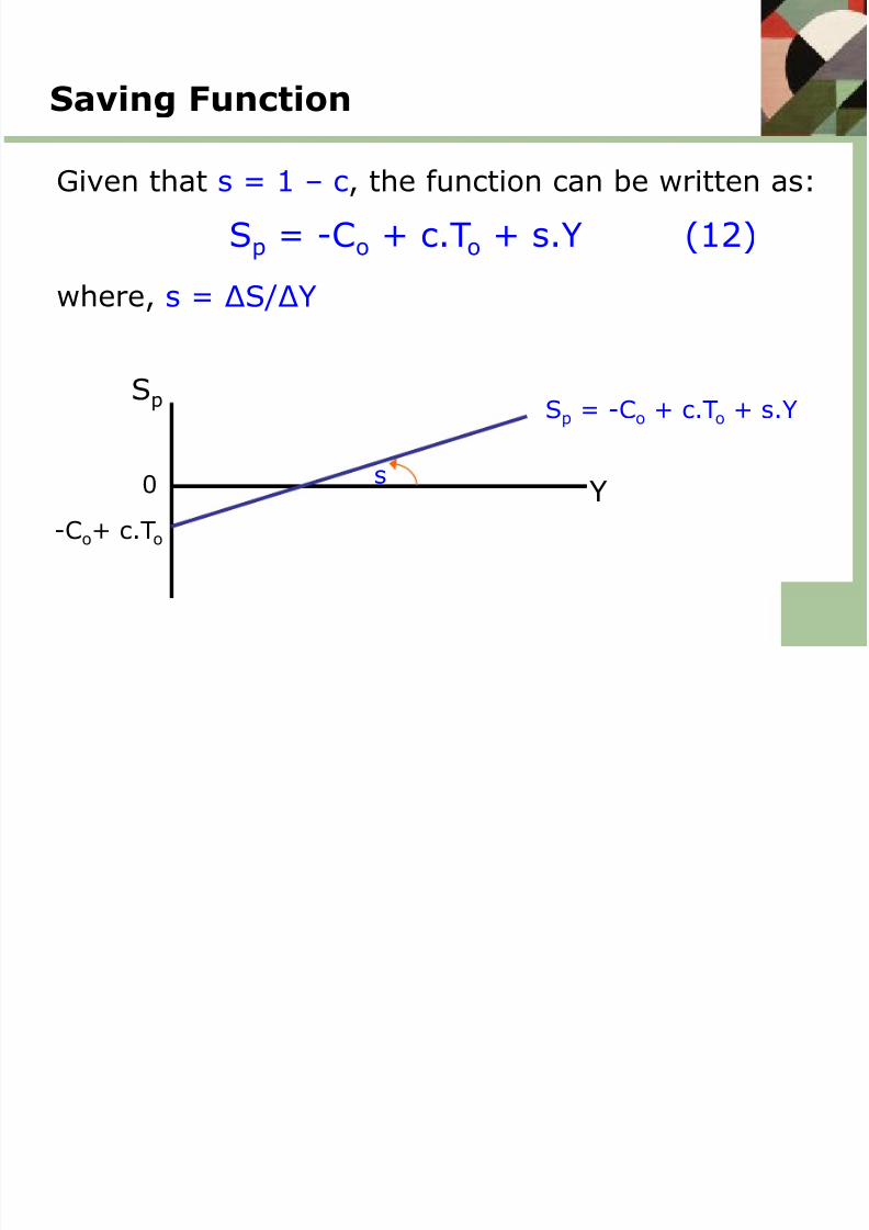
Given that s = 1 – c, the function can be written as:

Sp = -Co + c.To + s.Y (12)

where, s = ∆S/∆Y

Sp

0 Y

-Co+ c.To

s

Sp = -Co + c.To + s.Y



Autonomous Expenditure

Private investment and government spending are

determined independently of current levels of

aggregate income:

Ip = Io (13)

G = Go (14)

and, from (7):

A = Io+ Go + Co - c.To (15)

where A is autonomous expenditure.



Aggregate Demand Function

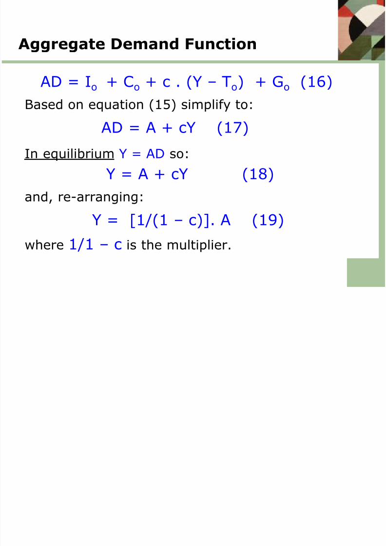
AD = Io + Co + c . (Y – To) + Go (16)

Based on equation (15) simplify to:

AD = A + cY (17)

In equilibrium Y = AD so:

Y = A + cY (18)

and, re-arranging:

Y = [1/(1 – c)]. A (19)

where 1/1 – c is the multiplier.



Explaining Autonomous Demand

• A feature of this model often overlooked is that thecomponents of autonomous demand, A (see equation 15),influence each other in their determination and that of A. Forexample, government expenditure can in certain circumstancesinfluence the level of private investment and, vice-versa,thereby affecting the total level of autonomous demanddetermined.

• But whereas the relationship between (endogenous)consumption and income is functional , as determined by thepropensity to spend (the multiplier for a given A), therelationship between Io, Co and Go in their determination and

that of A is contingent on wider circumstances.

• Notwithstanding the non-functional nature of the relationshipbetween the components of autonomous demand, explainingthem can be important in fully understanding economic issuesand policy options.



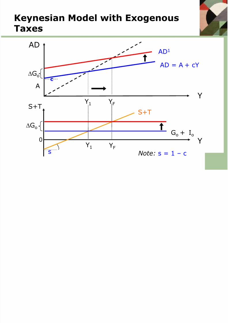
Keynesian Model with ExogenousTaxes

Y

Y

Y1

AD

S+T

Note: s = 1 – c

0

A

S+T

AD = A + cY

Y1 s

YF

YF

Go

Go

AD1

Go + Io

c



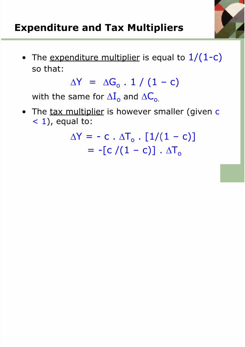
Expenditure and Tax Multipliers

• The expenditure multiplier is equal to 1/(1-c) so that:

Y = Go . 1 / (1 – c)

with the same for Io and Co.

• The tax multiplier is however smaller (given c< 1), equal to:

Y = - c . To . [1/(1 – c)]

= -[c /(1 – c)] . To



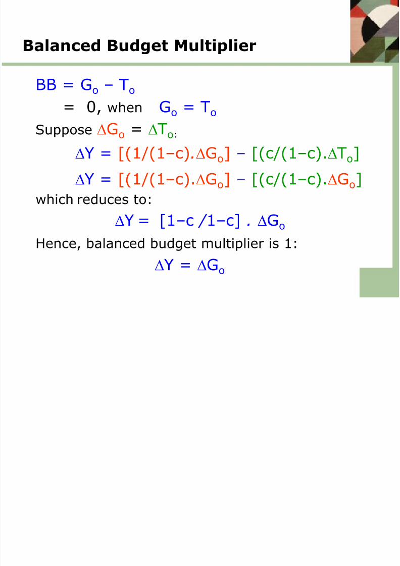
Balanced Budget Multiplier

BB = Go – To

= 0, when Go = To

Suppose Go = To:

Y = [(1/(1–c).Go] – [(c/(1–c).To]

Y = [(1/(1–c).Go] – [(c/(1–c).Go]

which reduces to:

Y = [1–c / 1–c] . Go

Hence, balanced budget multiplier is 1:

Y = Go



Balanced Budget Theorem

• The theorem states that because the governmentexpenditure multiplier is greater than the tax multiplier anexpansion in government spending matched by an equalincrease in taxes, has a positive multiplier effect on income,ceteris paribus.

• The reason for this is that government spending addsdirectly to aggregate demand (in the first round) whereasan increase in taxes reduces aggregate demand indirectly(in the first round) through lower consumption with some ofthe tax burden on households absorbed by lower saving.

• An implication is that generally fiscal policy is more effectivewhen acting on government spending than taxation.

Example: Suppose c = 0.8, Go= To = $100m.



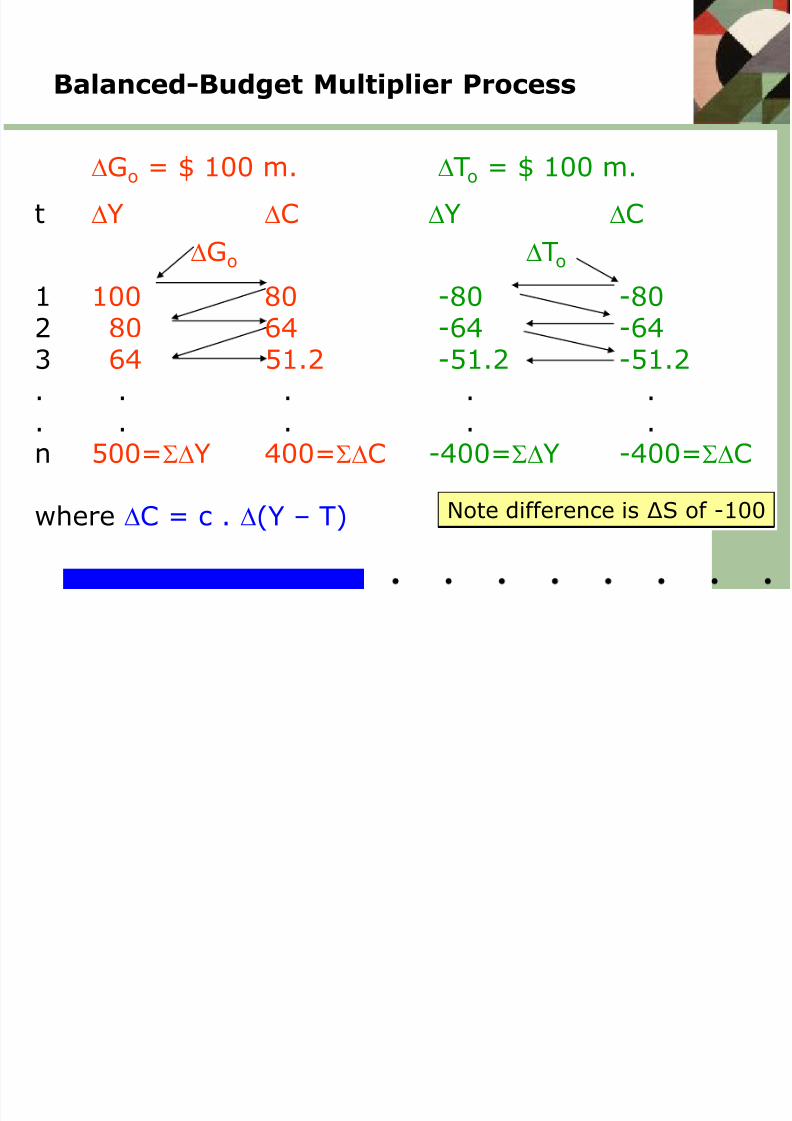
Go = $ 100 m. To = $ 100 m.

t Y C Y C

Go To

1 100 80 -80 -80 2 80 64 -64 -64 3 64 51.2 -51.2 -51.2. . . . .

. . . . .n 500=Y 400=C -400=Y -400=C

where C = c . (Y – T)

Balanced-Budget Multiplier Process

Note difference is ∆S of -100



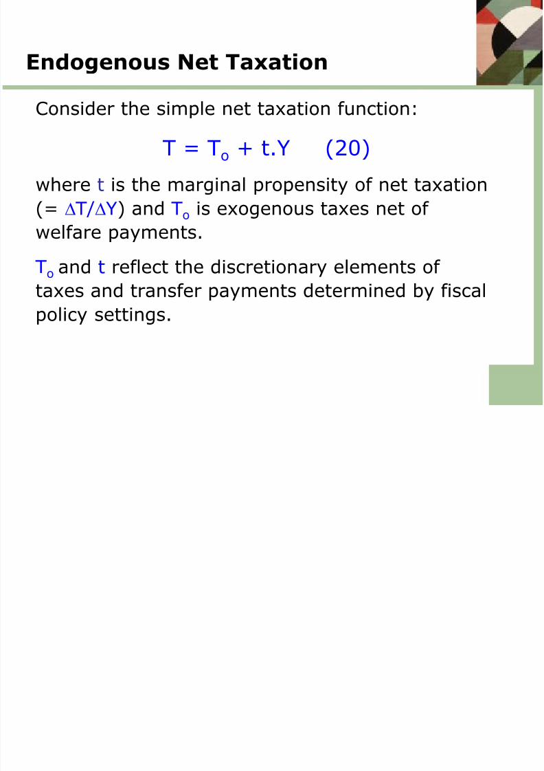
Endogenous Net Taxation

Consider the simple net taxation function:

T = To + t.Y (20)

where t is the marginal propensity of net taxation(= T/Y) and To is exogenous taxes net of

welfare payments.

To and t reflect the discretionary elements of

taxes and transfer payments determined by fiscalpolicy settings.



Model with Endogenous Net Taxes

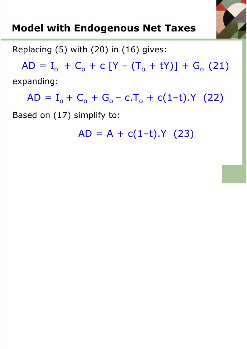
Replacing (5) with (20) in (16) gives:

AD = Io + Co + c [Y – (To + tY)] + Go (21)

expanding:

AD = Io + Co + Go – c.To + c(1–t).Y (22)

Based on (17) simplify to:

AD = A + c(1–t).Y (23)



Model with Endogenous Net Taxes

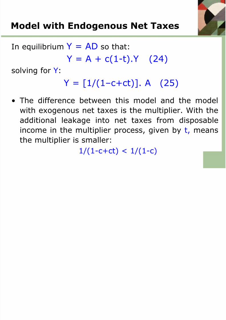
In equilibrium Y = AD so that:

Y = A + c(1-t).Y (24)

solving for Y:

Y = [1/(1–c+ct)]. A (25)

• The difference between this model and the model

with exogenous net taxes is the multiplier. With the

additional leakage into net taxes from disposableincome in the multiplier process, given by t, means

the multiplier is smaller:

1/(1-c+ct) < 1/(1-c)



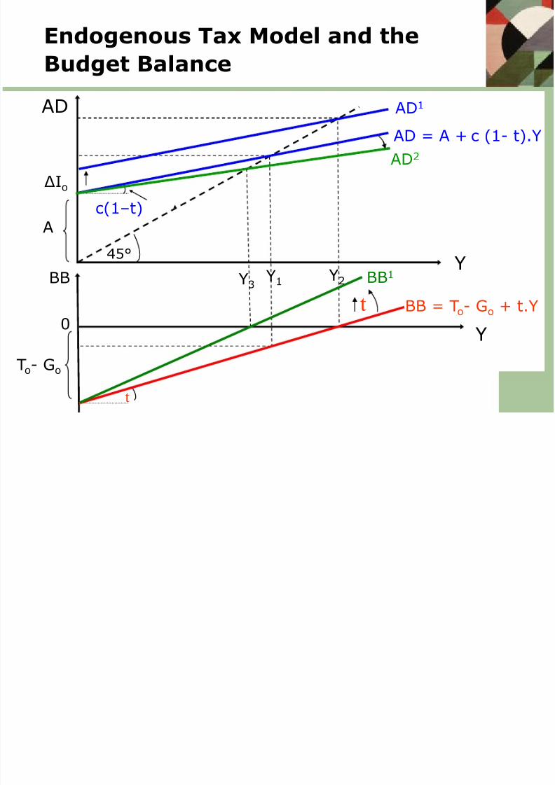
Endogenous Tax Model and the

Budget Balance

Y

Y

Y2

AD

BB

t

A

BB = To- Go + t.Y

AD = A + c (1- t).Y

∆Io

c(1–t)

To- Go

0

45°

Y1 BB1

AD1

t

Y3

AD2



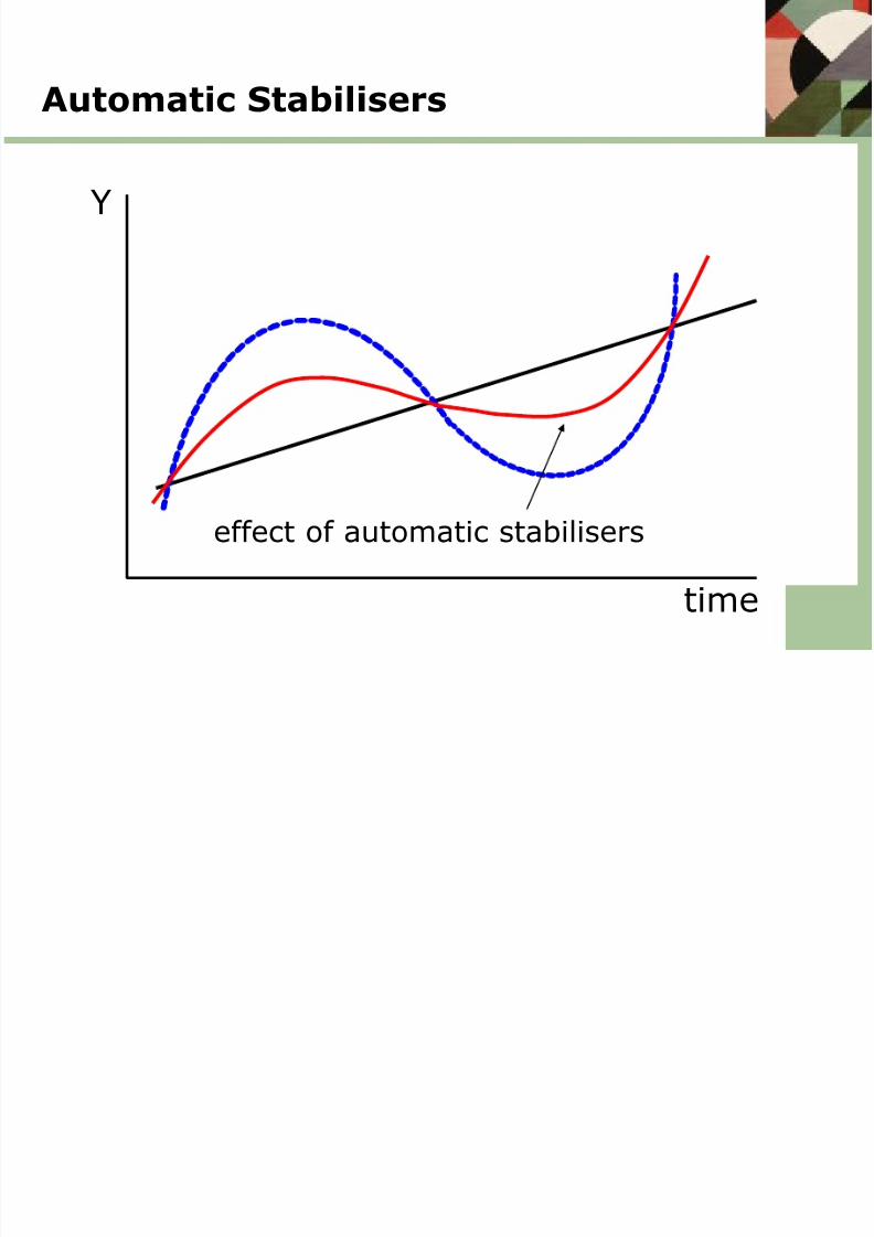
Automatic Fiscal Stabilisers

• Pro-cyclical nature of endogenous net taxationhas a stabilising effect on aggregate income.

• Stabilising effect is typically greater the larger

and more progressive the welfare state:– higher average t lower average multiplier

so that amplitude of business cycle ismoderated

– endogenous pro-cyclical variations in t itself( and multiplier) with the plausible assumptionthat t is an increasing function of Y, that is:

t = f (Y) see diagrams below



Automatic Stabilisers

effect of automatic stabilisers

Y

time



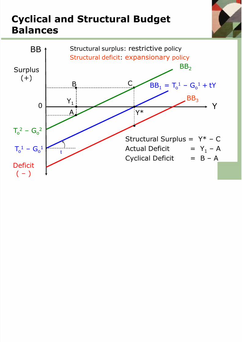
Fiscal Policy Stance

• The budget balance (BB) is dependent on, as wellas affecting, the state of the economy.

• Actual BB is not an indicator of the stance of fiscalpolicy - reflecting discretionary actions of fiscalpolicymakers; i.e. reflecting Go, To and t inequation: BB = [To+ tY] – Go

• Actual BB = Cyclical BB + Structural BB(Y) = (Y– Y*) + (Y*)

where Y* is average or natural level of income.

• Cyclical BB is due to variations in income whichcauses endogenous changes in net taxes (i.e. tY)and structural BB reflects discretionary policy

actions.



Cyclical and Structural BudgetBalances

A

BB1 = To1

– Go1

+

tY

YY*

Y1 0

t

BB

Surplus(+)

Deficit

( – )

BB2

B C

To1 – Go

1

To2 – Go

2

Structural Surplus = Y* – C

Actual Deficit = Y1 – A

Cyclical Deficit = B – A

BB3

Structural surplus: restrictive policy

Structural deficit: expansionary policy



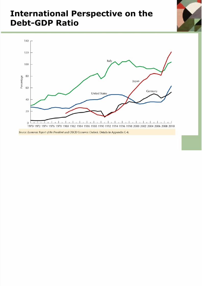
Fiscal Policy and Public Debt

• A potential constraint on fiscal policy is the size ofpublic debt or, more correctly, the debt-servicingcapacity of the national government.

• Capacity to service debt often measured by publicdebt/GDP ratio or by debt-servicing cost/revenueratio.

• Rule of thumb for debt-servicing: g > i, where g isgrowth rate and i is interest rate on bonds.

• Issue: Does i rise with size of public debt or debt/GDP?

• Much recent focus on fiscal polices to reduce publicdebt and how best to do it?





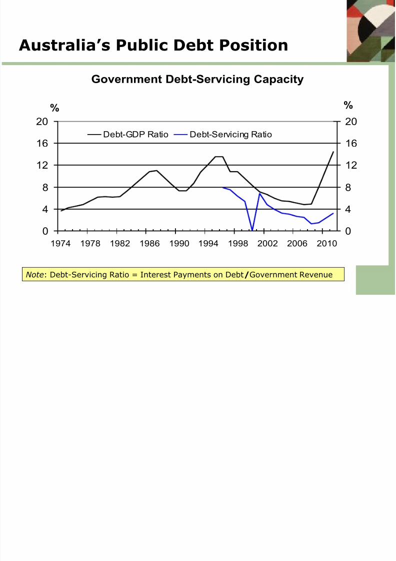
Australia’s Public Debt Position

Government Debt-Servicing Capacity

0

4

8

12

16

20

1974 1978 1982 1986 1990 1994 1998 2002 2006 2010

%%

0

4

8

12

16

20

Debt-GDP Ratio Debt-Servicing Ratio

Note: Debt-Servicing Ratio = Interest Payments on Debt/Government Revenue



Fiscal Policy and Public Debt Debate

• Since the global financial crisis of 2008, and withthe ongoing Euro-zone debt crisis, debate hasfocussed on fiscal policy and tackling high publicdebt in the midst of economic stagnation.

• Questions: Fiscal austerity versus fiscal stimulus?Does the ‘Euro’ debt problem stem from the ‘architecture’ of Euro-zone (i.e. EMU)?

• In Australia public debt is not a serious issue giventhe low debt-GDP ratio of 14%, compared to most

other OECD countries with ratio’s ranging between40-140%

• Question: Would budget deficit and public debt ofAustralia (and other countries) have been higherwithout post-2008 fiscal stimulus?



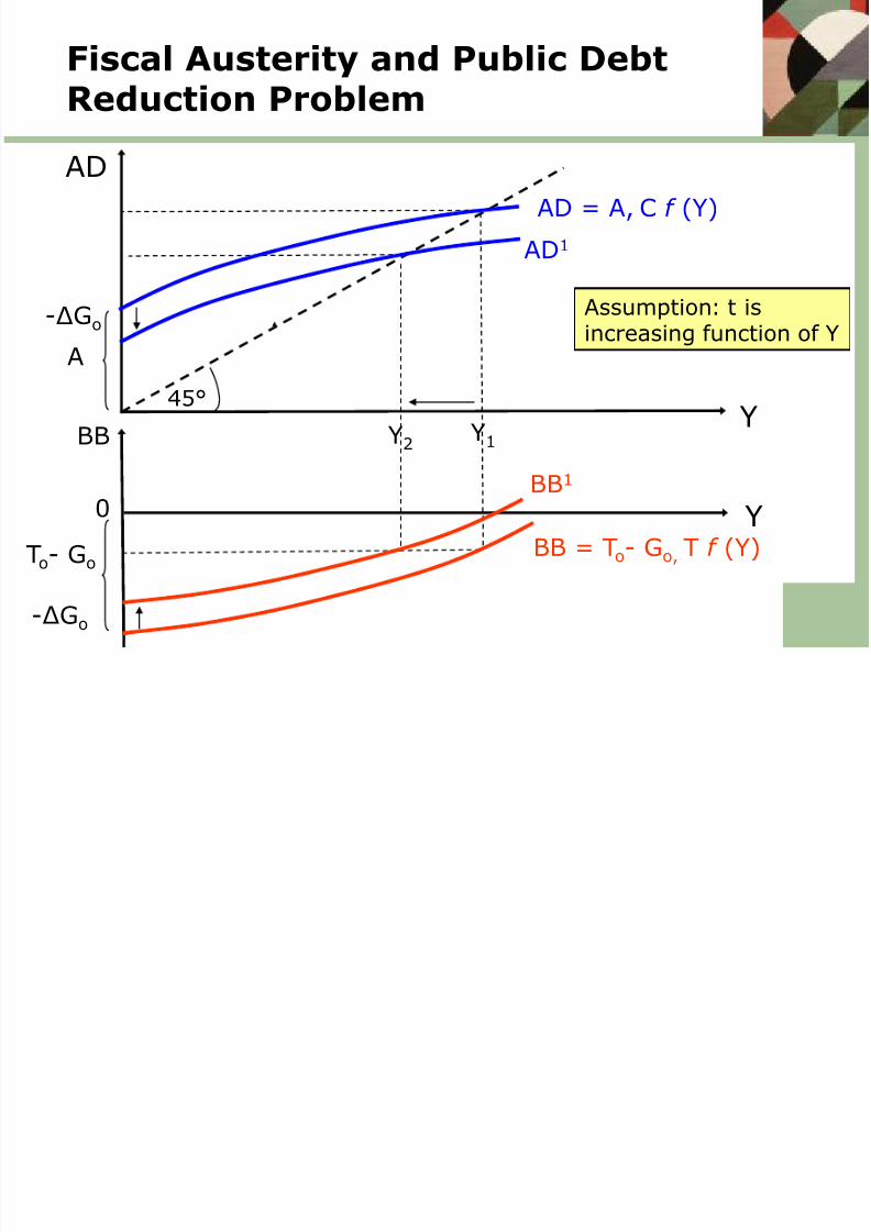
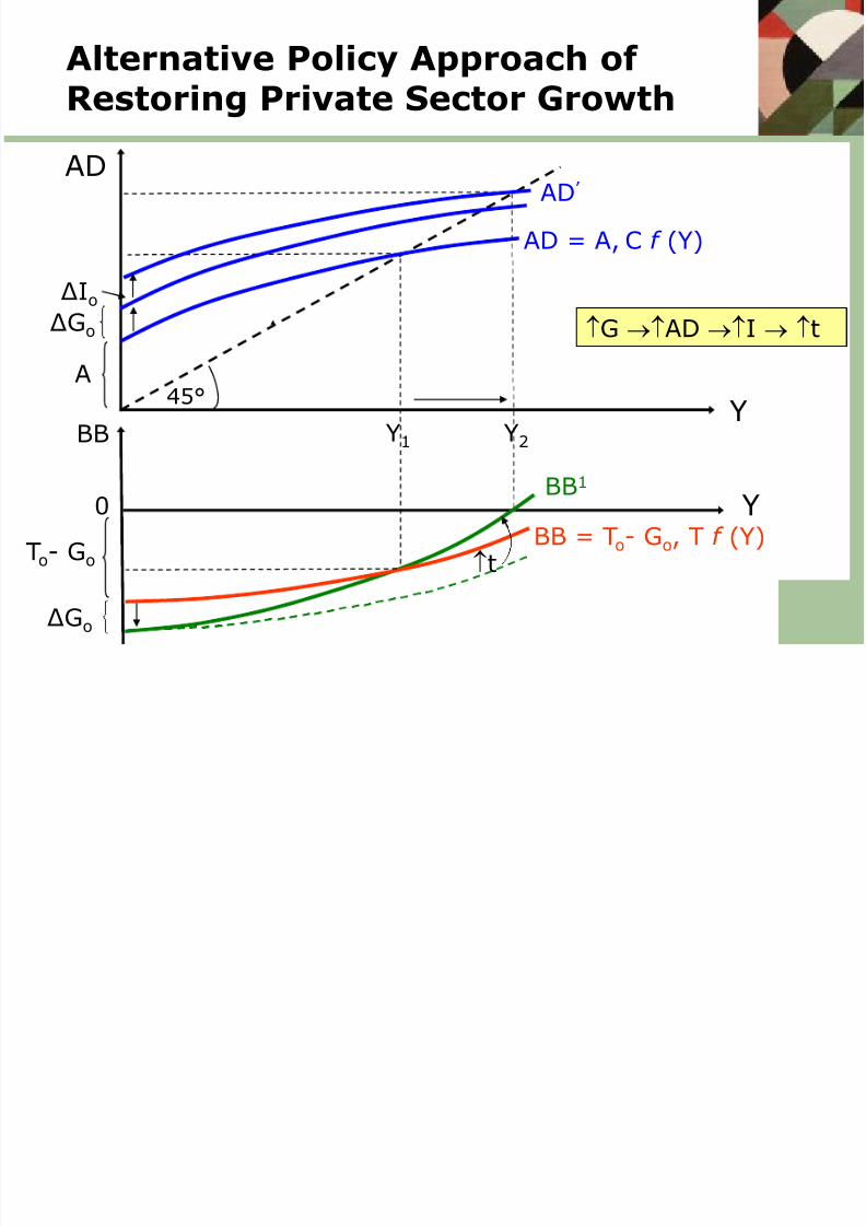
Fiscal Austerity and Public DebtReduction Problem

Y

Y

Y2

AD

BB

A

BB = To- Go, T f (Y)

AD = A, C f (Y)

-∆Go

To- Go

0

45°

-∆Go

Y1

BB1

AD1

Assumption: t isincreasing function of Y





Open Economy Model

AD = Cp + Ip + G + X – M (26)

whereX is exports and M is imports.

Note that [Cp+Ip+G–M] is domestic

demand, whereas [Cp+Ip+G] is domestic

demand for domestically produced goods.



Exports

Exports are determined by factors exogenous ofdomestic income:

X = Xo (27)

Exports depend mainly on two factors:1. the level of aggregate demand and, therefore,

income, in the rest of the world, Yw; and

2. relative price competitiveness of domestic

products compared to those produced in the restof the world, measured by the real exchange rateindex, e.

Hence: X = f (Yw, e) (28)



Imports

Imports mainly depend on domestic income asexpressed in the following function:

M = Mo + m.Y (29)

where

Mo is exogenous imports, largely influenced byinternational competitiveness (i.e. e)

m is the marginal propensity to import(m=M / Y), so that mY is imports endogenous ofincome.

Hence: M = f (Y, e) (30)

O E A D d



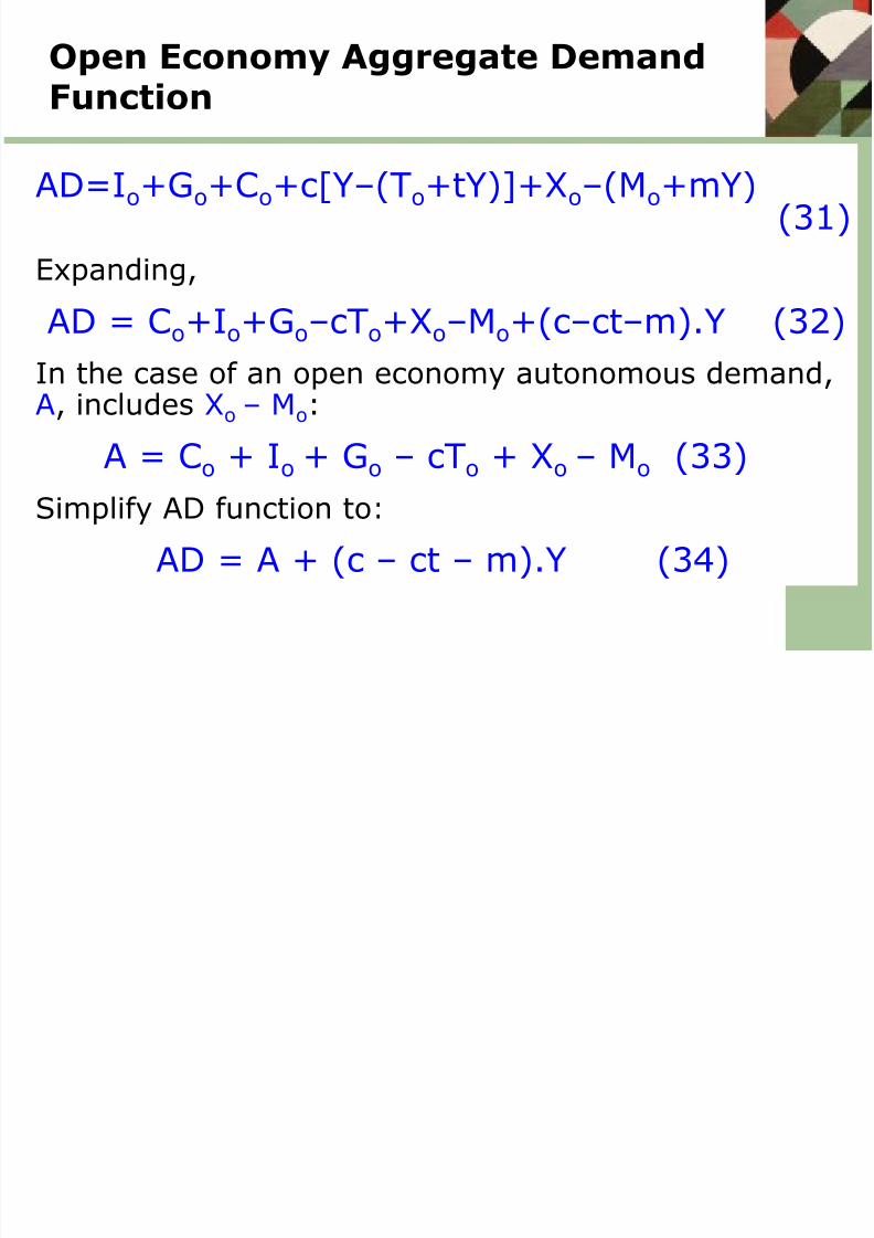
Open Economy Aggregate DemandFunction

AD=Io+Go+Co+c[Y–(To+tY)]+Xo–(Mo+mY)(31)

Expanding,

AD = Co+Io+Go–cTo+Xo–Mo+(c–ct–m).Y (32)

In the case of an open economy autonomous demand,A, includes Xo – Mo:

A = Co + Io + Go – cTo + Xo – Mo (33)Simplify AD function to:

AD = A + (c – ct – m).Y (34)

i i ilib i i



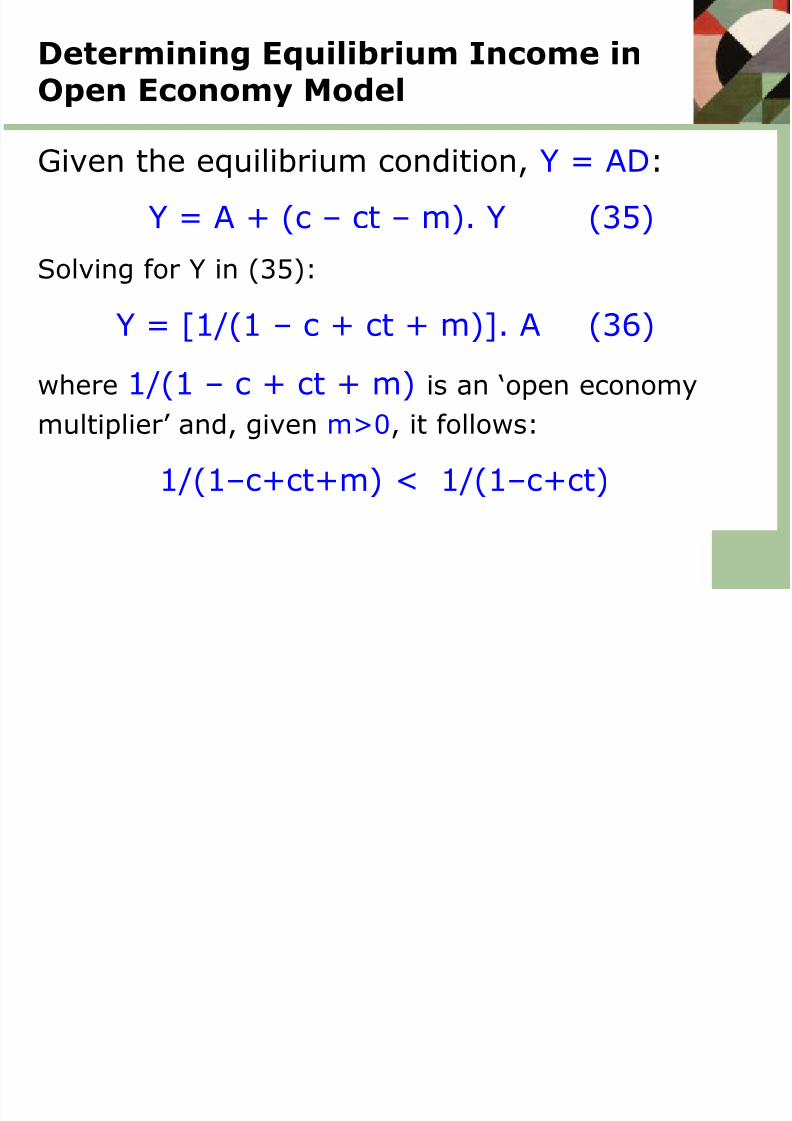
Determining Equilibrium Income inOpen Economy Model

Given the equilibrium condition, Y = AD:

Y = A + (c – ct – m). Y (35)

Solving for Y in (35):

Y = [1/(1 – c + ct + m)]. A (36)

where 1/(1 – c + ct + m) is an ‘open economy

multiplier’ and, given m>0, it follows:

1/(1–c+ct+m) < 1/(1–c+ct)



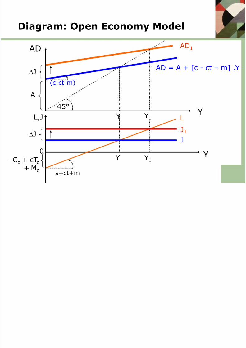
A

Diagram: Open Economy Model

J

Y

Y

AD

L,J

s+ct+m

L

AD = A + [c - ct – m] .Y

(c-ct-m)

45°

–Co + cTo

+ Mo

0

Y

Y

Y1

Y1

J

AD1

J1

J



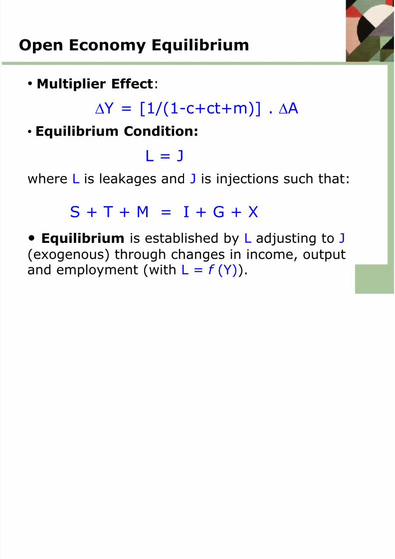
Open Economy Equilibrium

• Multiplier Effect:

Y = [1/(1-c+ct+m)] . A

• Equilibrium Condition:

L = J

where L is leakages and J is injections such that:

S + T + M = I + G + X

• Equilibrium is established by L adjusting to J

(exogenous) through changes in income, outputand employment (with L = f (Y)).



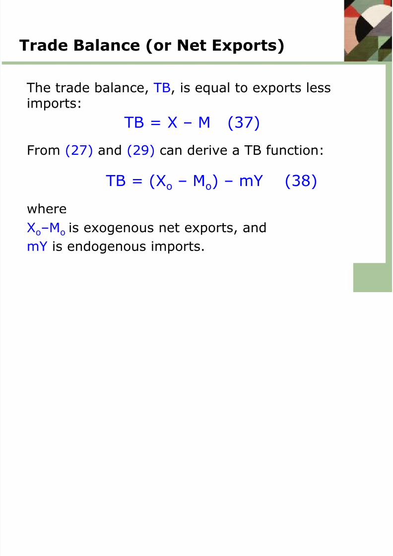
Trade Balance (or Net Exports)

The trade balance, TB, is equal to exports lessimports:

TB = X – M (37)

From (27) and (29) can derive a TB function:

TB = (Xo – Mo) – mY (38)

whereXo–Mo is exogenous net exports, and

mY is endogenous imports.

Mac oeconomic Polic and the



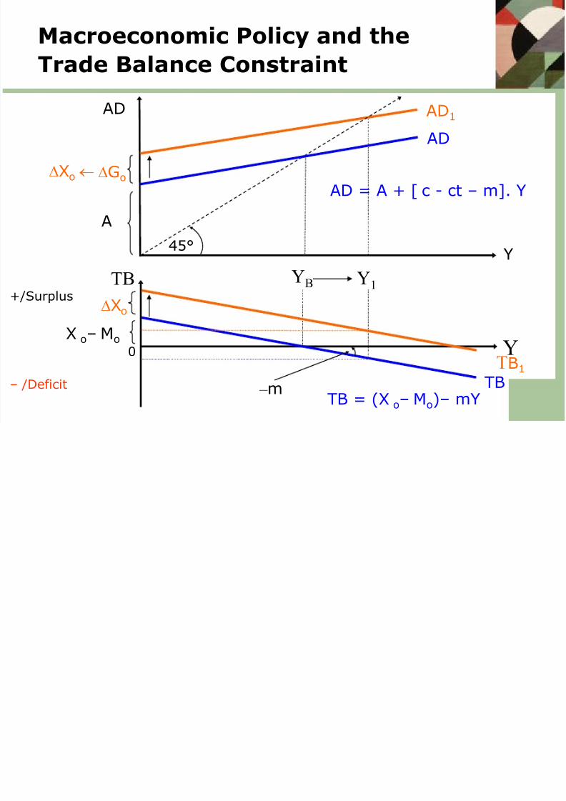
Macroeconomic Policy and the

Trade Balance Constraint

Y1

AD1

Go

AD

0

Y

Y

AD

m

A

45°

X o– Mo

YBTB+/Surplus

– /Deficit TB

AD = A + [ c - ct – m]. Y

TB1

Xo

Xo

Documents

Macro Economics Introuction