7

ISSN 1392-1258. EKONOMIKA 2014 Vol. 93(4)

MACROECONOMIC DETERMINANTS OF LITHUANIAN GOVERNMENT SECURITY PRICES

Linas Jurkšas*, Rūta KropienėVilnius University, Lithuania

Abstract. This paper deals with the impact of macroeconomic fundamentals on Lithuanian government se-curities’ prices using quarterly data for the period 2000–2013, applying five major macroeconomic variables: gross domestic product, consumer prices, interest rates, money supply, and foreign direct investment. The two main goals of the paper are: 1) to identify macroeconomic variables which are the main driving forces behind debt security prices and 2) due to the lack of sufficient data on the Lithuanian government security index, to create and calculate a similar index from the primary and secondary market sovereign security prices. The re-search has been conducted using the methods of descriptive statistics, the vector autoregression model, the impulse response function, and the forecast error variance decomposition. The paper finds that, when consu-mer prices or interest rate rise up, sovereign security prices decline significantly and, on the other hand, money supply is the only factor that significantly and directly influences the government security prices. However, the effects of the gross domestic product and foreign direct investment were found to be statistically insignificant. Finally, the government security index is inert and rarely changes its long-term trend. These conclusions pro-vide related persons with rich information in establishing the investment strategy or fiscal / monetary policy.

Key words: macroeconomic determinants, government security index, government security prices, vector au-toregression, impulse response function

1. Introduction

What are the main driving forces behind debt security prices? Is it liquidity or credit risk? Or are debt securities more affected by changing the term structure of yields, downgrade / upgrade of credit rating, or even speculation? Until recently, most of the researchers have come to the above-mentioned conclusions. However, since the start of the last financial crisis, empirical studies about the transmission of macroeconomic forces to debt security prices gained momentum. The reason is simple – the crisis has revealed that countries with big fiscal or monetary imbalances and poor macroeconomic fundamentals experienced the surge of their borrowing costs. So, the interest to reassessing the relationship between macroeconomic forces and government security prices is renewed.

The demand for government securities from emerging markets is rapidly increasing due to international investors who search for higher returns and / or diversification benefits. As

* Corresponding author:Vilnius University, Faculty of Economics, Sauletekio Ave. 9, LT-10222 Vilnius, Lithuania.E-mail: l.jurksas@gmail.com.

8

a result, the last two decades witnessed a considerable increase in the issuance of sovereign bonds in these markets. However, emerging markets experience unique, country-specific macro risks that sometimes lead to internal economic crises, e.g., the Asian crisis of 1997, the Russian crisis of 1998 or the Argentinian crisis of 2000. So, one can expect that the relationship between country-specific factors and government securities in emerging markets is much tighter than in developed countries, and the examination of these ties is extremely important for both investors and for policy-makers.

However, most of the studies concentrate on the sovereign security markets in most de-veloped countries, while literature on emerging markets is relatively scarce. Besides, few single-country studies analyse markets other than the USA, and Lithuania, one of the fast-est growing economies in Europe, is no exception. In order to close this gap, we contribute to the existing literature on the macroeconomic factors that affect Lithuanian sovereign security prices. The macro factors in our empirical framework include interest rates, infla-tion, money supply, gross domestic product, and foreign direct investment. We employ the most popular and advanced quantitative methods used in similar studies, such as vector autoregression, impulse response functions, and forecast error variance decomposition.

The structure of this paper is as follows. Since the relationship between macroeconomic fundamentals and government securities is not obvious, the next (second) chapter summarises relevant theory and literature. In the third chapter, we describe the main econometric models to investigate the impact of macroeconomic factors on government security prices. The results of the graphical and econometrical analysis are considered and interpreted in the fourth chapter. Finally, we draw conclusions and make suggestions for the future studies.

2. Review of theory and literature

There are far fewer academics who examine the impact of macroeconomic factors on debt securities than on other assets, e.g., stocks or real estate. This is due to the fact that the impact is not an obvious one – not all authors come to the conclusion that only macro determinants explain debt security prices. For instance, Mody, 2009; Schuknecht et al., 2010 and others find empirical evidences against country-specific macroeconomic fundamentals. According to them, other factors such as international risk factors, liquidity and credit risk or even behaviour finance (i.e. changing risk aversion) are the main drivers behind changing yields. Others (Nelson and Siegel, 1987; Svensson, 1995) analyse yield curve factors and term structure to determine the forces affecting bond prices.

However, Arghyrou and Kontonikas (2012) find that, unlike in the pre-crisis period when markets rarely priced macro fundamentals, markets have been pricing macroeconomy heavily during and after the crisis, and several factors, notably monetary and fiscal policy, have become principal determinants of yields. During the most recent financial crisis,

9

almost all countries of the European Union have been experiencing large increases in their spreads versus Germany due to deteriorating economic fundamentals and the ‘flight-to-quality’ from poorly balanced countries. So, according to Arghyrou and Kontonikas (2012), since 2007 the movements of macro and fiscal fundamentals explain sovereign debt price movements well and in the way consistent with theoretical expectations.

Piljak (2013) analysed the relative importance of global versus domestic factors in fourteen countries and found that domestic macro plays a more important role than global fundaments in explaining bond returns. Specifically, the domestic inflationary environment and monetary policy were identified as the most significant factors that affect returns. His additional finding is the thesis that during the crisis markets have been penalising macroeconomic imbalances much more heavily than before.

In pursuit to reconcile approaches of different authors, some assess the role of an extended set of potential factors, including both macro and bond-specific ones. For example, Alfonso et al. (2012) examined such determinants as macroeconomic and fiscal factors, international risk (i.e. the implied volatility of the US stock index), crisis transmission risk, liquidity conditions, and credit ratings. They have found that, unlike in the period preceding the global financial crisis, the European government bond prices are well explained by macroeconomic factors and that macro risks have become significantly more important. Moreover, Xie, Shi and Wu (2008) suggest that even the yield term structure models should include macroeconomic factors to capture the default premium and to explain changes of bond yields more successfully.

One of the most cited articles that investigate the interaction between macroeconomy and bond prices is written by Ludvigson and Ng (2009). They conclude that macro factors explain up to 44% of all variation in excess US government bond returns, so with accurate and timely information one could predict the future bond prices and earn a higher return. Especially, production and unemployment were found to be the most significant determinants in explaining bond returns. However, particular attention in similar studies is mostly attributed to monetary policy. For example, Evans and Marshall (1998) state that even though the effect of monetary policy is not so trivial, the tightening of this policy strongly reduces debt prices.

In general, the main driving macro forces behind debt prices that most of the authors examine are interest rates, inflation, money supply, economic activity, investment, and others. Obviously, the principal fundamental that affects debt security prices is the interest rate. According to Ilmanen (1995), the return of debt security is driven by several factors, and bonds issued by a government that has almost no insolvency or cash flow risk are mainly affected by the interest rate risk. The increasing rates signal the decrease of the ability of the government to refinance and service the debt in the future, so the return required by investors is simultaneously increased and ultimately bond prices

10

fall. This effect becomes more apparent when bonds are compared to other investment options. For example, if the interbank interest rate increases, the interest rate of deposits will also rise – if government bond yields do not increase, investors would simply direct more funds to deposits, in which case the demand of bonds would still decline. Also, it should be mentioned that in accordance with the expectations theory supported by Koukouritakis and Michelis (2008), long-term government bond yields are a function of current and expected short-term rates, so the monetary policy that sets these rates is extremely important for bond investors.

One of the most comprehensive papers that describe the effects of inflation is written by Reilly and Brown (2000). They state that increasing prices could severely affect bond prices if, of course, they are not indexed to inflation. This occurs when the rise (decline) of inflation puts an upward (downward) pressure on the required return of investors who want to keep the same real return on investment. In the case of emerging markets, inflation is also showed to be a leading indicator of the balance of payment crises and as a proxy for the quality of economic management thus directly influencing the sovereign default risk. This effect is particularly known due to the rule of Taylor (1993) who states that a 1% increase in inflation should prompt the central bank to raise the nominal interest rate by more than 1%, which should undoubtedly negatively affect the government bond prices. In addition, the increase of money supply can lead to a higher inflation in the future, so the quantity of money can predict the future consumer price movements and have the same effect on debt securities as inflation has. However, a share of increased money supply can be dirrected to debt securities markets, i.e. increasing the demand and the prices, so the final effect is not an obvious one.

According to Cochrane and Piazzesi, 2005; Gerlach et al., 2010, the return of a bond can be predicted as a response to economic activity. When the economic situation of a country improves, the government can reduce the amount of debt issued and, as a result, also the supply of government securities, so prices should grow and yields decline. If the economic situation has deteriorated, the yields could soar – this risk is especially apparent in emerging markets that occasionally experience ‘sudden stops’. Thus, the ‘health’ of the country’s economy and the change of credit worthiness have a direct impact on bond prices. However, under certain circumstances, the opposite effect is also possible. When the rapid growth of the national economy puts an upward pressure on inflation, the monetary policy could be tightened, i.e. the money supply could be reduced and/or interest rates increased – the effect of procyclical covariance was the argument of above-mentioned Taylor (1993). In this case, since most of government securities are not indexed to inflation, the demand and prices of these securities should fall.

The foreign direct investment (FDI) should have a direct effect on asset (including debt securities) prices. The rapidly inflowing FDI implies that the country has brighter

11

future prospects, so its creditworthiness improves and yields decline. Moreover, the growing FDI usually positively correlates with portfolio investments that direct money to all kinds of assets – stocks, real estate, and bonds. However, Chowdhury, Bayar, and Kilic (2013) examined the FDI impact on bond index values of 25 emerging countries and found a reverse effect, so the growing FDI not always translates into lower bond prices.

It should be mentioned that, although other macroeconomic factors also have an influence on government security, their importance is lower or they are directly related to the above-mentioned factors. For instance, Chee and Fah (2013) examined the impact of the exchange rate on bond yields, and the results showed that the strengthening of the pound sterling in relation to the US dollar had a positive effect on the UK government bond yields, possibly due to the changes of inflation expectations. Even the size of a country can play an important role in shaping the demand of government securities – Beber et al. (2009) found that the smaller the country, the relatively lower demand for government securities is, so it is more difficult for smaller countries to raise capital than for big ones. The increasing public debt and deficits should reduce government security prices – a conclusion reached by Faini, 2006; Bernoth et al., 2004 who studied the relationship between the European debt levels and yields. An interesting finding of the level of debt was reached by Gnabo and Bernal (2010) – to a certain extent (from 36% to 106% of GDP for different European countries) increasing government debt reduces yields, but above this threshold the yields start rising sharply. Moreover, even though such domestic indicators as the rate of unemployment, net export or reserves of a country could affect the government security prices, their importance is generally much lower.

The literature assessing the impact of the Lithuanian macroeconomic factors on government securities is very limited or attributed to analysing many emerging countries at once. One of such examples is a study by Alexopoulou, Bunda, and Ferrando (2009) who examined new states of the European Union and found that the main macro determinants behind the Lithuanian government security prices were inflation and foreign trade. They concluded that since the start of the financial crisis the fundamental-based yields have been on a rising path, and this trend is likely to continue.

3. Methods and data used in the analysis

3.1. Vector autoregression model, impulse response function, and forecast error variance decomposition

In order to analyse the impact of the Lithuanian macroeconomic factors on sovereign security prices, we employ the Sims (1980) vector autoregression (VAR) model. This model is not a single equation (as in the case of the autoregression model), but a system.

12

Each equation describes the formation of a different variable by using not only its own variable delays, but also all other variables and their delays in this equation system. Due to the fact that the VAR model is appropriate for multidimensional models, it helps to analyse connections among numerous variables (e.g., macroeconomic versus financial) simultaneously.

The simplest VAR model can be described by two equations:

Yt = β10 – β11×Zt + γ11×Yt–1 + γ12×Zt–1 + εYt, (1)

Zt = β10 – β21×Yt + γ21×Yt–1 + γ22×Zt–1 + εZt, (2)

where: Yt, Zt (in the left side) are endogenous variables (in this study the government security

index),Yt, Zt (in the right side) are exogenous variables (in this study – macroeconomic

indicators), β, γ are the coefficients in search,ε are the shocks of an equation (innovations).

This model is just for two variables, but it can be easily extended to a larger number of variables under examination; in this case, the number of equations must equal the quantity of variables. The presented model is called a structural VAR model which shows the economic relations among the variables: coefficient β11 reveals the instantaneous impact of variable Z on Y, and β21 shows the instantaneous impact of variable Y on Z. Thus, in order to discover the causal relationships among the variables, it is necessary to examine whether the coefficients are significantly different from 0.

One of the most important tasks in getting the correct standard (not yet structural) VAR model is to choose the lag length. This step can be done with the help of information criteria (IC). The most commonly used IC are Akaike (AIC), Schwarz (SC), and Hannan Quinn (HQ) – the lowest value of IC shows what lag size should be chosen. This value should be selected carefully, because the bigger the lag length, the higher the possibility to reduce the explanatory power of the model due to the loss of the degrees of freedom. However, a standard VAR model (the discovery of which has been described above) does not have a lot of economic sense, so it is necessary to transform it to a structural VAR. This is done through the reverse A matrix (in this study the size of 6×6) with the diagonal splitting (coefficients of zero). Finally, after a structural VAR equation is found, it is necessary to check the statistical significance of variables.

VAR models are widely used in examining whether macroeconomic factors play an important role in explaining changes of asset prices. For instance, Ameer, 2007; Chang, Chen and Chou, 2011 use a VAR approach to find such relations. As a complement they

13

also use impulse response functions. This method helps to identify what the impact on variable is in t, t + 1, t + 2, etc. periods from a shock (innovation) that happened in the t–1 period of another variable. The assumptions of this model are that this shock completely disappears in the next period and that the shocks of all other variables are equal to 0.

Let’s say that we are examining the same two variables defined in equations (1) and (2). If we want to check how the shock of variable Z affects not only itself, but also variable Y, then we have to enter the Z shock into the equation describing the Y variable:

Yt = β10 – β11 × Zt + γ11 × Yt–1 + γ12 × Zt–1 + εYt + εZt. (3)

It should be mentioned that the easiest way to analyse the results of this method is with the use of the impulse response graph which visually shows how a shock of a variable affects another variable many periods hereafter.

However, in order to determine the relative importance of such shock, impulse response functions are not enough. The analysis of forecast error variance decomposition (FEVD) can help to solve this task. It shows the scale of the effect from shocks of different variables in distinct periods. This method assists by measuring the ratio of the change that separates the shocks of different variables (Enders, 1995). As in the case of impulse response functions, it is most convenient to analyse the FEVD graphically.

The VAR model is especially suitable for the analysis of stationary data. However, most of financial time series are non-stationary – without any adjustment it is possible to deal with a spurious regression. So, it is important to identify the order of integration before analysing the effects that macroeconomic factors cause to sovereign securities. Usually, this is done by using the augmented Dickey–Fuller (ADF) unit root test. With the help of this test, the estimated ADF value of each variable is compared with the critical value in a certain confidence interval – if the calculated statistics is lower than the critical Dickey–Fuller value, the null hypothesis, stating that the process has a unit root, i.e. is non-stationary, can be rejected and the alternative conclusion that the existing process is stationary accepted. In addition to the ADF test, Phillips and Perron (hereinafter – PP) in 1988 developed a non-parametrical unit root test. This test is more conservative in measuring the order of integration, pays less attention to the number of lags (which significantly alters the results of ADF test) and more suitable when errors are heteroskedastic – this often happens in the context of financial and economic variables.

3.2. Data used in the analysis

After examination of similar studies on the role that macro fundamentals play in driving debt security prices, five economic indicators were chosen as independent variables: gross domestic product, foreign direct investment, the harmonized index of consumer prices, money supply, and interbank interest rate (a brief description is presented in

14

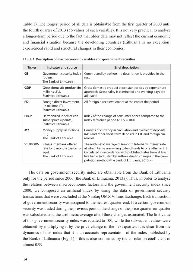
Table 1). The longest period of all data is obtainable from the first quarter of 2000 until the fourth quarter of 2013 (56 values of each variable). It is not very practical to analyse a longer-term period due to the fact that older data may not reflect the current economic and financial situation because the developing countries (Lithuania is no exception) experienced rapid and structural changes in their economies.

TABLE 1. Description of macroeconomic variables and government securities

Ticker Indicator and source Brief description

GS Government security index (points).The Bank of Lithuania

Constructed by authors – a description is provided in the text

GDP Gross domestic product (in millions LTL).Statistics Lithuania

Gross domestic product at constant prices by expenditure approach. Seasonality is eliminated and working days are adjusted

FDI Foreign direct investment (in millions LTL).Statistics Lithuania

All foreign direct investment at the end of the period

HICP Harmonized index of con-sumer prices (points).Statistics Lithuania

Index of the change of consumer prices compared to the index reference period (2005 = 100)

M2 Money supply (in millions LTL). The Bank of Lithuania

Consists of currency in circulation and overnight deposits (M1) and other short-term deposits in LTL and foreign cur-rencies

VILIBOR6 Vilnius Interbank offered rate for 6 months (percent-age). The Bank of Lithuania

The arithmetic average of 6-month Interbank interest rate at which banks are willing to lend funds to one other in LTL. Calculated in accordance with published rates from at least five banks (adjusted by authors due to changes in the com-putation method (the Bank of Lithuania, 2013b))

The data on government security index are obtainable from the Bank of Lithuania only for the period since 2006 (the Bank of Lithuania, 2013a). Thus, in order to analyse the relation between macroeconomic factors and the government security index since 2000, we composed an artificial index by using the data of government security transactions that were concluded at the Nasdaq OMX Vilnius Exchange. Each transaction of government security was assigned to the nearest quarter-end. If a certain government security was traded during the previous period, the change of the price quarter-on-quarter was calculated and the arithmetic average of all these changes estimated. The first value of this government security index was equated to 100, while the subsequent values were obtained by multiplying it by the price change of the next quarter. It is clear from the dynamics of this index that it is an accurate representation of the index published by the Bank of Lithuania (Fig. 1) – this is also confirmed by the correlation coefficient of almost 0.99.

15

In this study, we transform daily, monthly or quarterly data into quarterly time series. Quarterly data are used by many other authors (e.g., Chowdhury, Bayar, and Kilic, 2013; Chionis, Pragidis and Schizas, 2014; and others). Moreover, when the variables are changing at a relatively constant rate, it is recommended to transform them into a linear form by using logs of such data (Enders, 1995). For this reason, we use the values of the government security index as well as macroeconomic variables (except VILIBOR) in logarithm.

4. Analysis of the impact of macroeconomic factors on government securities prices

4.1. Graphical analysis

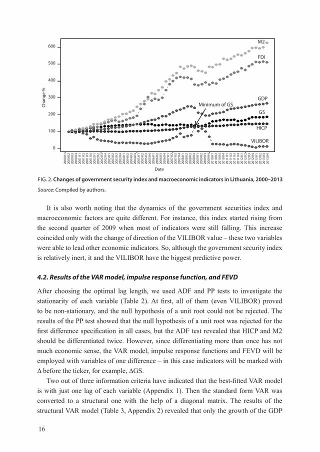
During the period, the government securities index was rising almost entirely with a low volatility (Fig. 2), so this index is very inert and continues its long-term trend. The only exception is the decline in 2008–2009 when this index fell by almost 10%, although most of other asset classes and macroeconomic variables in Lithuania fell much harder – obviously, the government securities give a diversification benefit. This is consistent with the classical portfolio management theory which says that debt securities reduce the profitability of the investment portfolio when the economy is growing, but at least partially they absorb losses from riskier asset classes when the economic situation is getting worse.

80

90

100

110

120

130

140

I II III IV I II III IV I II III IV I II III IV I II III IV I II III IV I II III IV I II III IV

2000 2001 2002 2003 2004 2005 2006 2007

Index published by the Bank of Lithuania Index calculated by authors from the transaction data

FIG. 1. Changes of the Bank of Lithuania index and the index calculated by authors from the tran-saction data

Sources: Bank of Lithuania and authors calculations.

16

It is also worth noting that the dynamics of the government securities index and macroeconomic factors are quite different. For instance, this index started rising from the second quarter of 2009 when most of indicators were still falling. This increase coincided only with the change of direction of the VILIBOR value – these two variables were able to lead other economic indicators. So, although the government security index is relatively inert, it and the VILIBOR have the biggest predictive power.

4.2. Results of the VAR model, impulse response function, and FEVD

After choosing the optimal lag length, we used ADF and PP tests to investigate the stationarity of each variable (Table 2). At first, all of them (even VILIBOR) proved to be non-stationary, and the null hypothesis of a unit root could not be rejected. The results of the PP test showed that the null hypothesis of a unit root was rejected for the first difference specification in all cases, but the ADF test revealed that HICP and M2 should be differentiated twice. However, since differentiating more than once has not much economic sense, the VAR model, impulse response functions and FEVD will be employed with variables of one difference – in this case indicators will be marked with Δ before the ticker, for example, ∆GS.

Two out of three information criteria have indicated that the best-fitted VAR model is with just one lag of each variable (Appendix 1). Then the standard form VAR was converted to a structural one with the help of a diagonal matrix. The results of the structural VAR model (Table 3, Appendix 2) revealed that only the growth of the GDP

GDP

GS

FDI

HICP

VILIBOR

Minimum of GS

M2600

500

400

300

200

100

0

Chan

ge %

Date

2000

K1

2000

K2

2000

K3

2000

K4

2001

K1

2001

K2

2001

K3

2001

K4

2002

K1

2002

K2

2002

K3

2002

K4

2003

K1

2003

K2

2003

K3

2003

K4

2004

K1

2004

K2

2004

K3

2004

K4

2005

K1

2005

K2

2005

K3

2005

K4

2006

K1

2006

K2

2006

K3

2006

K4

2007

K1

2007

K2

2007

K3

2007

K4

2008

K1

2008

K2

2008

K3

2008

K4

2009

K1

2009

K2

2009

K3

2009

K4

2010

K1

2010

K2

2010

K3

2010

K4

2011

K1

2011

K2

2011

K3

2011

K4

2012

K1

2012

K2

2012

K3

2012

K4

2013

K1

2013

K2

2013

K3

2013

K4

FIG. 2. Changes of government security index and macroeconomic indicators in Lithuania, 2000–2013

Source: Compiled by authors.

17

and money supply has a positive instantaneous impact on the value of the government security index, but only the impact of money supply is statistically significant. These effects are so minor probably due to increasing inflationary expectations – this is also confirmed by the results of the influence of inflation and interest rates which are significantly negative. The impact of FDI on sovereign security prices is very small and insignificant.

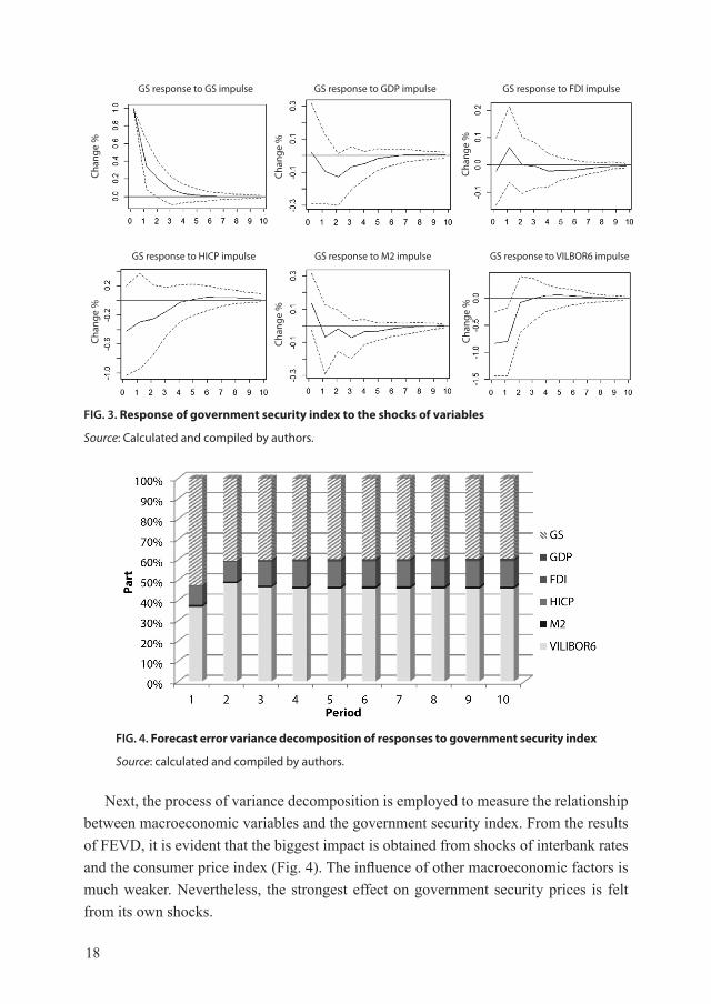
The impulse response functions revealed that the evolution of a standard deviation unit shock of five macro factors has long-lasting effects on the government security index (Fig. 3). Noticeable oscillations could be detected even after three quarters since the shock occurred. Moreover, the effects are pretty permanent and negative, the only exception being a positive response to its own shock. In the first period, the government security prices also positively respond to FDI changes, but this effect is small and reverses in the next period. After the shock of GDP, the government security index declines six, after HICP four, after M2 nine and after VILIBOR three quarters onwards. Thus, in the long term the government security prices react negatively not only to a higher inflation, but also to the improvements of the economic situation.

TABLE 2. Results of the unit root test of the government security index and macroeconomic variables*

Ticker Lag ADF value PP valueADF value

(first difference)PP value

(first difference)

GS 1 1.8929 -1.6511 -4.1971 -4.6962

GDP 1 2.3768 -1.0608 -3.9269 -4.8909

FDI 1 2.5397 -1.7878 -4.2639 -5.2583

HICP 4 1.0973 0.2931 -1.33 -4.7815

M2 4 0.7212 -2.2864 -1.0845 -6.5338

VILIBOR6 2 -1.703 -1.8546 -3.646 -7.4759

*Critical ADF value is -1.95 and critical PP value is -2.91at 95% confidence interval.

Source: authors’ calculations.

TABLE 3. Estimation of the VAR(1) model

Ticker ∆GDP ∆FDI ∆HICP ∆M2 ∆VILIBOR6

∆GS+0.02%

(0.31)-0.02%(-0.72)

-0.42%(-2.84)*

+0.12%(2.56)*

-0.92%(-6.64)*

Note: calculated t statistics are written below the estimates and the effects that are statistically significant are marked with *.

Source: calculated by authors.

18

Next, the process of variance decomposition is employed to measure the relationship between macroeconomic variables and the government security index. From the results of FEVD, it is evident that the biggest impact is obtained from shocks of interbank rates and the consumer price index (Fig. 4). The influence of other macroeconomic factors is much weaker. Nevertheless, the strongest effect on government security prices is felt from its own shocks.

FIG. 3. Response of government security index to the shocks of variables

Source: Calculated and compiled by authors.

FIG. 4. Forecast error variance decomposition of responses to government security index

Source: calculated and compiled by authors.

GS response to GS impulse GS response to GDP impulse GS response to FDI impulse

GS response to HICP impulse GS response to M2 impulse GS response to VILBOR6 impulse

Chan

ge %

Chan

ge %

Chan

ge %

Chan

ge %

Chan

ge %

Chan

ge %

19

4.3. Summary of the results

As one can see from the graphical analysis and the results of various employed models, macroeconomic fundamentals have a predictive power for government security prices. When the latest macroeconomic data are published or accurately predicted, it is possible to foresee the future variations of government security prices. This opportunity should be valuable not only to economists and investors who are looking for the most efficient way to rebalance their investment portfolios, but also to policy-makers who are responsible for making well-grounded decisions in the monetary or fiscal policy. After all, refinancing debt is a costly ‘pleasure’ that needs good timing and understanding of the main price drivers.

First of all, the government security index is quite inert – the effect of its own shocks is direct and accounts for over 40% of all the forecast error variance. The impact of the impulses lasts over a year. This trend was also clearly noticeable from the graphical analysis – although the variance was not big, the prices followed their own trend which changed only several times. In addition, this security is an appropriate investment when the economic situation deteriorates.

Most of the analysed macroeconomic determinants have an inverse effect on government security prices (Table 4). This is especially true with HICP and VILIBOR – when these variables increase, the government security prices decrease by 0.42 to 0.92%. This result should not be surprising as investors discount the estimated future cash flows in order to calculate the value of government security – the rising interest rates increase the investors’ required return. While the Lithuanian sovereign security are not indexed to inflation, increasing consumer prices worsen the outlook of the government security prices. These findings coincide with the results of other researchers who have analysed how inflation and interest rates affect debt security in other countries (Alexopoulou, Bunda, Ferrando, 2009; Piljak, 2013). So, it was no surprise that from the middle of 2009 when banks could borrow ‘cheaper’ money from each other (as can be seen from the graphical analysis), the government security prices were growing rapidly. As it is evident from FEVD, despite the very impulse from government securities, the greatest impact on prices is caused by HICP and VILIBOR shocks.

TABLE 4. The results of the effects of variables on government security prices

VariableMethod

GS GDP FDI HICP M2 VILIBOR6

VAR   +0.02% -0.02% -0.42%* +0.12%* -0.92%*Impulse response f. + - ~ - - -Importance of the variable (FEVD) 1 6 5 3 4 2

Note: * indicates the significant influence; a long-term (at least a few periods) trend is marked in case of the impulse response function; the importance of the variable (FEVD) indicates the relative importance in the first period in the FEVD model (1 – most significant, 6 – least significant).

Source: authors’ calculation.

20

Money supply has the strongest instantaneous direct impact on government security prices. This can be related to the fact that a share of the increased money supply is probably directed not only to the riskiest assets, but also to debt securities. However, the results of impulse response functions prove that this effect is not unambiguous as the rapid growth of money supply finally leads to higher inflation expectations. This risk automatically transforms to higher discount rates and, consequently, to lower government security prices. So, in the long term, investors should search for more profitable investments.

Two other macroeconomic factors – output and foreign investment – make the smallest effects on the government security prices. This finding suggests that the increase of GDP and FDI can confuse investors: on the one hand, improvement in economic activity reduces the risk of insolvency; on the other hand, it increases the risk of inflation. Moreover, this can be explained by the fact that, during the rise of economic activity attraction to riskier investments grows as well. However, these two indicators are not as important as monetary policy – the same conclusions were made by Poghosyan, 2012 and Piljak, 2013.

5. Conclusions

The main macroeconomic determinants that drive government security prices were discussed in this paper. Five macroeconomic factors that are most widely used in similar researches are interest rates, changes of consumer prices, money supply, domestic product, and foreign direct investment. Quarterly data from 2000 to 2013 were used. This study has solved the problem of insufficient data of the Lithuanian government security index by calculating an artificial one from the primary and secondary market government security prices.

We employed the most commonly used and advanced methods to analyse the relations between financial and macro factors: the vector autoregression model, the impulse response function, and the forecast error variance decomposition. The government security index and all macroeconomic indicators were found to be non-stationary, so in the further analysis the first differences of variables were used.

The majority of macroeconomic factors make an inverse impact on the Lithuanian government security prices. In the background of rising inflation and / or interest rates, sovereign security prices decline. Money supply is the only factor that directly and significantly affects government security prices. The effects of the gross domestic product and foreign direct investment are statistically insignificant and not as clear as the influence of the monetary policy.

The countercyclical nature of government securities implies that it is a suitable investment when the macroeconomic situation deteriorates. Also, the government security index is quite inert and not very variable, so in the long run a sound fiscal and

21

monetary policy remains imperative for anchoring lower borrowing costs. Thus, our findings offer investors and policy-makers rich and valuable information in assessing the role of macroeconomic fundamentals in driving government security prices.

In the future, it would make sense to analyse the impact of macroeconomic factors with different frequency data, such as monthly or annual. Moreover, interesting conclusions could be drawn by comparing the results of different economic cycles (economic upturn versus downturn).

REFERENCES

Alfonso A., Arghyrou, M.G. and Kontonikas, A. (2012). The determinants of sovereign bond yield spreads in the EMU. Working Paper of School of Economics and Management, Vol. 36.

Ameer R. (2007). What moves the primary stock and bond markets? Influence of macroeconomic factors on bond and equity issues in Malaysia and Korea. Journal of Accounting and Finance, Vol. 3, No. 1, p. 93–116.

Arghyrou, M.G., Kontonikas, A. (2012). The EMU sovereign debt crisis: Fundamentals, expectations and contagion. Journal of International Financial Markets, Institutions and Money, Vol. 22, p. 658–677.

Beber, A., Brandt, M.W., Kavajecz, K.A. (2009). Flight-to-quality or flight-to-liquidity? Evidence from the Euro-area bond market. The Review of Financial Studies, Vol. 22, p. 925–957.

Bernoth, K., von Hagen, J., Schuknecht, L. (2004). Sovereign risk premia in the European government bond market. ECB Working Paper, 369.

Bhansali, V. (2011). Bond Portfolio Investing and Risk Management. McGraw-Hill. Brinson, G. P., Singer, B. D., Beebower, G. L. (1991). Determinants of Portfolio Performance II: An

Update. Financial Analyst Journal, Vol. 47, issue 3.Chee, S.W., Fah, C.F. (2013). Macro-economic determinants of UK treasury bonds spread.

International Journal of Arts and Commerce, Vol. 2, issue 1.Chang, C.Y., Chen, C.Y., Chou, J.H. (2011). Empirical evidence on the causality among yield curve

factors and macroeconomic determinants. International Review of Accounting, Banking and Finance, Vol. 3, issue 3, p. 48–69.

Chen N. (1991). Financial investment opportunities and the macroeconomy. Journal of Finance, Vol. 46, issue 2, p. 529–554.

Chionis, D., Pragidis, I., Schizas, P. (2014). Long-term government bond yields and macroeconomic fundamentals: Evidence for Greece during the crisis-era. Finance Research Letters.

Chowdhury, Z.I., Bayer, Y., Kilic, C. (2013). Effects of major macroeconomic indicators on emerging markets bond index. IIBF Dergisi, S. II.

Cochrane, J.H., Piazzesi, M. (2008). Decomposing the yield curve. Working paper, Chicago Booth.Dickey, D. A., Fuller, W. A. (1981). Likelihood ratio statistics for autoregressive time series with a

unit root. Econometrica, Vol. 49, p. 1057–1072.Enders, W. (1995). Applied Econometric Time Series. John Wiley and Sons.Evans, C. L., Marshall, D. A. (1998). Monetary policy and the term structure of nominal interest

rates: Evidence and theory. Carnegie-Rochester Conference Series on Public Policy, Vol. 49, p. 53–111.Faini, R. (2006). Fiscal policy and interest rates in Europe. Economic Policy, Vol. 21. Gerlach, S., Schulz, A., Wolff, G. (2010). Banking and sovereign risk in the euro area. CEPR

Discussion Paper, Vol. 7833.Gnabo, J.Y., Bernal, O. (2012). Sovereign bond spreads: the role of debt accumulation. Center for

Research in Finance and Management.

22

Ilmanen, A. (1995). Time-varying expected returns in international bond markets. Journal of Finance, Vol. 50, issue 2, p. 481–506.

Koukouritakis, M., Michelis, L. (2008). The term structure of interest rates in the 12 newest EU countries. Applied Economics, Vol. 40, issue 4, p. 479–490.

Ludvigson, S. C., Ng, S. (2009). Macro factors in bond risk premia. Review of Financial Studies, Vol. 22, p. 5027–5067.

Mody, A. (2009). From bear sterns to Anglo-Irish: How Eurozone sovereign spreads related to financial sector vulnerability. IMF Working Paper, 09/108.

Nelson, C.R., Siegel, A.F. (1987). Parsimonious modelling of yield curves. Journal of Business, Vol. 60, issue 4, p. 473–489.

Perron, P. (1990). Testing for a unit root in a time series with a changing mean. Journal of Business and Economic Statistics, Vol. 8, p. 153–162.

Phillips, P. C., Perron, P. (1988). Testing for a unit root in time series regression. Biometrika, Vol. 75, p. 335–346.

Piljak, V. (2013). Bond markets co-movement dynamics and macroeconomic factors: Evidence from emerging and frontier markets. Emerging Markets Review, Vol. 17, p. 29–43.

Reilly, F., Brown, K. (2000). Investment Analysis and Portfolio Management. Dryden Press, 6th edition.

Schuknecht, L., von Hagen, J., Wolswijk, G. (2010). Government bond risk premiums in the EU revisited: The impact of the financial crisis. ECB Working Paper, 1152.

Sims, C.A. (1980). Macroeconomics and reality. Econometrica, Vol. 48, p. 1–48.Sims, C. A., Stock, J. H., Watson, M. W. (1990). Inference in linear models with some unit roots,

Econometrica, Vol. 58.Svensson, L. (1995). Estimating forward interest rates with extended Nelson & Siegel Method.

Sveriges Riksbank Quarterly Review, Vol. 3.Taylor, J.B. (1993). Discretion versus policy rules in practice. Carnegie–Rochester Conference,

Series on Public Policy. Vol. 39, p. 195–214.The Bank of Lithuania (2013a). Naujas indeksas atskleis kaip vertinama Lietuvos finansinė būklė.

http://www.lb.lt/naujas_indeksas_atskleis_kaip_vertinama_lietuvos_finansine_bukleThe Bank of Lithuania (2013b). Nauja vidutinių tarpbankinių palūkanų normų skaičiavimo tvarka

leis tiksliau atspindėti padėtį rinkoje. http://lb.lt/nauja_vidutiniu_tarpbankiniu_palukanu_normu_skaiciavimo_tvarka_leis_tiksliau_

atspindeti_padeti_rinkojeXie, Y.A., Jian, S., Wu, C. (2008). Do macroeconomic variables matter for pricing default risk?

International Review of Economics and Finance, Vol. 17, p. 279–291.

APPENDIX 1. Calculation of values of the VAR model

Lag 1 2 3 4AIC(n) 8.500199 8.754366 8.801392 8.618244HQ(n) 9.108135 9.883389 10.451503 10.789443SC(n) 10.091114 11.708922 13.119591 14.300084FPE(n) 4967.4424 6790.7967 8327.8445 9621.0776

23

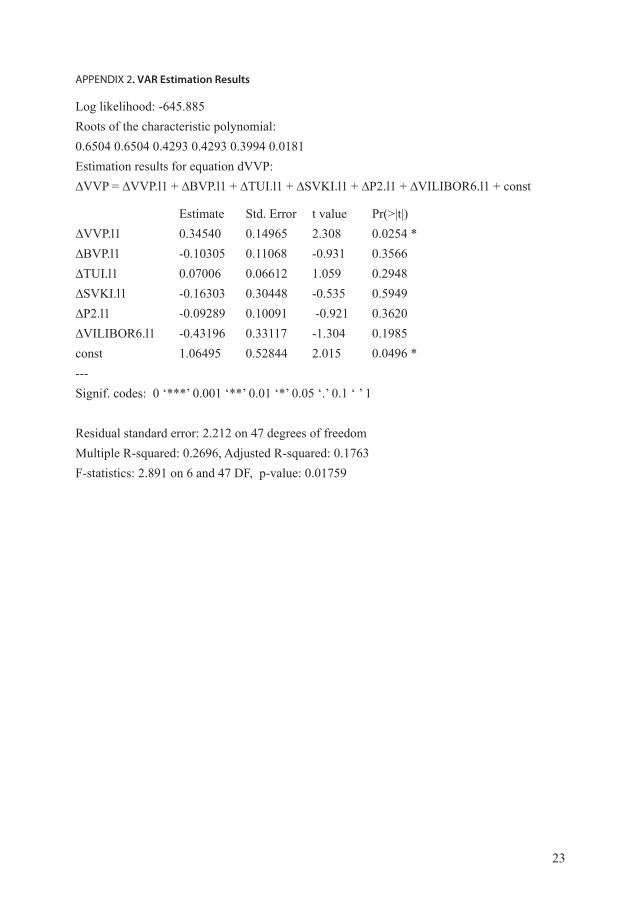
APPENDIX 2. VAR Estimation Results

Log likelihood: -645.885 Roots of the characteristic polynomial:0.6504 0.6504 0.4293 0.4293 0.3994 0.0181Estimation results for equation dVVP: ∆VVP = ∆VVP.l1 + ∆BVP.l1 + ∆TUI.l1 + ∆SVKI.l1 + ∆P2.l1 + ∆VILIBOR6.l1 + const

Estimate Std. Error t value Pr(>|t|) ∆VVP.l1 0.34540 0.14965 2.308 0.0254 *∆BVP.l1 -0.10305 0.11068 -0.931 0.3566 ∆TUI.l1 0.07006 0.06612 1.059 0.2948 ∆SVKI.l1 -0.16303 0.30448 -0.535 0.5949 ∆P2.l1 -0.09289 0.10091 -0.921 0.3620 ∆VILIBOR6.l1 -0.43196 0.33117 -1.304 0.1985 const 1.06495 0.52844 2.015 0.0496 *---Signif. codes: 0 ‘***’ 0.001 ‘**’ 0.01 ‘*’ 0.05 ‘.’ 0.1 ‘ ’ 1

Residual standard error: 2.212 on 47 degrees of freedomMultiple R-squared: 0.2696, Adjusted R-squared: 0.1763 F-statistics: 2.891 on 6 and 47 DF, p-value: 0.01759