Macroeconomic Effects of Fiscal Policy Changes: A Case of

OA Akanbi / Economic Modelling 35 (2013) 771-785

Macroeconomic Effects of Fiscal Policy Changes: A Case of South Africa

By Olusegun Ayodele Akanbi (Corresponding Author)

Associate Professor (Economics)

University of South Africa Pretoria, South Africa

Postal Address: Economics Department

PO Box 392 UNISA South Africa, 0003

Email: [email protected] or

[email protected]

Telephone: +27124334637

Dr. Olusegun Ayodele Akanbi is an Associate Professor of Economics at the University of South Africa. He holds a PhD in Economics with specialisation in macro-econometric modelling from the University of Pretoria. He is an academia with a private sector experience in quantitative analysis. He worked for Pan-African Investment & Research Services (PAIRS), Johannesburg in the capacity of a Senior Economist & Head of Research. He has also worked for the Department of Strategic Policy and Review at the International Monetary Fund (IMF) Washington D.C. focusing on debt sustainability among the low-income countries. Dr. Akanbi has led and participated in a number of major projects across South Africa.

mailto:[email protected]

mailto:[email protected]



Highlights of the Study

• Fiscal consolidation is contractionary on the economy in the short- to medium-term.

• Fiscal consolidation is more effective in an economy with no supply constraints.

• Purely expenditure changes are more effective in the absence of supply constraints.

• Purely tax revenue changes are more effective in the presence supply constraints.


- 1 -


Abstract This study develops comprehensive full-sector macro-econometric models for the South African economy with the aim of explaining and providing the macroeconomic effects of fiscal policy changes in the country. The models are applied to test the effectiveness of fiscal policy actions in an economic environment with existing structural supply constraints versus demand-side constraints and also to detect which components of the fiscal would be more effective in stabilising the economy. Based on the structure of the South African economy and the framework presented, the study concludes that the South African economy can be characterised as one which is embedded with structural supply constraints. Thus, a model which is suitable for policy analyses of the South African economy needs to capture the long-run supply-side characteristics of the economy. A price block is incorporated to specify the price adjustment between the supply-side sector and real aggregate demand sector. The models are estimated with time-series data from 1970 to 2011, capturing both the long-run and short-run dynamic properties of the economy. The results from the series of fiscal policy scenarios suggest that fiscal policy actions are more effective in an economic environment with limited or no supply constraints. Fiscal expansion or consolidation that comes more from government spending changes will be more effective in an economic environment where structural supply constraints are absent while tax revenue changes will be more effective in an economic environment where there exist major structural supply constraints.

JEL Classification: C51, C53, C32, E20, E62, H60

Keywords: Macro-Econometric Modelling, Macroeconomics, Fiscal Policy, South Africa


- 2 -

1. Introduction Fiscal policy remains an essential demand management tool of government in stabilising and stimulating economic activity. The last few years have experienced one of the biggest economic crises since the 1930s and the need to stabilise the global economy using fiscal and monetary policy tools became very urgent. This paper deals, however, only with fiscal policy measures.

The literature on fiscal policy changes and its effects on the macro economy are anchored on two different schools of thoughts. The classical view is that government expenditure will completely crowd out private investment and will not have any effect on the economy, while the Keynesian position is that fiscal policy actions are appropriate tools to stabilise the economy in the short-term. However, seminal works anchored on these strong positions have mixed results, with strong arguments in support of fiscal policy having a major impact on output and consumption, while others argue that fiscal policy changes do not have any effects on aggregate demand given that individuals smooth out their consumption pattern over time (Blanchard & Perotti, 1999; Ramsey, 2008; Dornbusch et al 1998; Blinder & Solow, 2005).

The role of fiscal policy in stabilising the South African economy cannot be underestimated given that about 30 per cent of aggregate domestic demand comes from government consumption expenditure and about 95 per cent of this expenditure is financed through tax revenue. Therefore, fiscal policy should play a big role in affecting the economy especially in the short- to medium-term.

Many empirical studies (Afonso & Sousa, 2012; Romer & Romer, 2010; Abbas et al 2010; Endegnanew et al 2012; Ocran, 2011; Gibson & Van Seventer, 1997; and Calitz, 2000) (inclusive of the South Africa case) have been carried out on the link between fiscal policy actions and other aspect of the economy such as GDP, employment, inflation and current account. These studies found a significant impact of fiscal policy (tax and expenditure changes) actions on the major macroeconomic variables. But there has been no strong empirical evidence to support the plausibility of which components of fiscal policy (tax or expenditure) would be more effective in stabilising the economy.

Based on the above background, the main objective of this study is to develop and estimate full-sector macro-econometric models for the South African economy1. The models are then applied to:

• Test the effectiveness of fiscal policy actions in an economy with existing structural supply constraints versus demand-side constraints; and

• Test the hypothesis of how fiscal consolidation which, comprises entirely of tax increases and fiscal consolidation which, is entirely from government expenditure cuts will be more effective on the macro economy.

This idea is partly a follow-up from the International Monetary Fund (IMF) (2011) and the current debates (outcome of the global economic crises) on what components of fiscal policy should consolidation come from. In this milieu, the study will enable policy

1 Similar approach has been established in Akanbi & Du Toit, (2011) when analysing the growth-poverty gap in Nigeria.


- 3 -

makers especially in South Africa to detect the kind of economic environment they operate in and which types of fiscal policy measures should be adopted.

The results suggest that fiscal consolidation typically has contractionary effects on economic activity especially in the short- to medium-term. Fiscal consolidation is found to be more effective in an economic environment with limited or no supply constraints. In addition, fiscal policy action that comes more from government spending changes will be more effective in an economic environment where structural supply constraints are absent while tax revenue changes will be more effective in an economic environment where major structural supply constraints exist.

The rest of the study is organised as follows: Section 2 evaluates the fiscal performance of the South African economy in which the structural and cyclical components of the budget are identified. Section 3 presents an empirical analysis which contains the model specification, methodology, data description, core structural equations, model closures and the fiscal policy simulations. Section 4 concludes the study, provides policy recommendations and highlights some limitations encountered in the study.

2. Evaluating the Fiscal Performance of the South African Economy –Some Stylized Facts The stylized facts presented in this section focus on revealing the fiscal performances of the South African economy over the past few decades. It detects the cyclicality of the fiscal policy actions and also reveals the components of the fiscal balances that are cyclical and structural in nature.

Fiscal policy actions have been much more linked to the economic performances than most other policies due to its direct and immediate effects on the economy. Counter-cyclical fiscal policies have been widely accepted in the literature as the most appropriate tool to stabilise the economy. Figure 1 shows the relationship between the fiscal balance as a percentage of GDP and the estimated output gap2.

The estimated curve shows that for every 6 percentage point change in output gap, the fiscal balance changes by approximately 2.4 percentage points (translating into a slope of 0.4) over the period 1970 to 20113. This reveals a counter-cyclical fiscal policy actions adopted in most of these years. The distribution in Figure 1 is well spread across the cyclical axis (output gap) but recorded fiscal deficits for all the years except for 20074.

2 Output gap is represented as the percentage deviation of actual GDP from potential GDP in relation to potential GDP. Potential GDP is estimated using the Hodrick-Prescott (HP) filter technique. This technique has been widely accepted as a robust estimate of the potential level of GDP and it’s important to note that, the potential output measured in this study do not represent output that could be produced under full employment conditions, but rather viewed it as the maximum output that can be produced without causing any inflationary pressures (Okun 1962; DeMasi 1997; and Klein 2011). 3 These estimates are similar to Swanepoel & Schoeman (2003). 4 Note that, series are in yearly 2005 prices which may be slightly different from the fiscal years.


- 4 -

Figure 1: Cyclicality of the Fiscal Balance (1970-2011)

Source: South African Reserve Bank and Author’s Own Calculation

The counter-cyclicality nature of fiscal policy actions in South Africa does not change after 1994 (end of apartheid). Breaking down the series into two components, the apartheid (1970-1993) and post-apartheid (1994-2011) fiscal policy revealed the same counter-cyclical policies with a slope of 0.15 in both periods.

In order to understand the implications of the changes in South Africa’s economic conditions in terms of fiscal measures, there is a need to break down the fiscal balance into structural and cyclical components. This breakdown is presented in Figure 2. Figure 2: Structural and Cyclical Fiscal Balance (1970-2011)

Source: South African Reserve Bank and Author’s Own Calculation


- 5 -

The cyclical component reflects the fiscal balance’s sensitivity to the cyclical condition of the economy due to the reaction of the automatic stabilisers, while the structural component is the difference between the cyclical and observed balances. To estimate the cyclical component, the BBVA (2012) approach to Spain data was adopted and is presented below:

Annual cyclical fiscal balance = Slope of curve in Figure 1(0.4) * Annual output gap

The series generated as presented in Figure 2 is similar to the alternative measure adopted in Endegnanew et al (2012) when trying to capture the non-policy factors suggested by the IMF (2011) as a weakness to the conventional approach to estimating the cyclical components. As shown in Figure 2, fiscal policy actions since 1970 have been mainly structural in nature with only about 15 per cent of the total fiscal balances on average to be attributed to cyclical fluctuations of the economy.

This scenario is different when comparing the apartheid and post-apartheid era. In the apartheid era, structural balances recorded about 113 per cent of the total fiscal balances, indicating that no policy actions were caused by the business cycle. In the post-apartheid era fiscal policy actions were, still counter-cyclical but recorded about 52 per cent cyclical component and 48 per cent structural on average. This swing was caused by the spike in 2007 (fiscal surplus year) and post-crisis (2007) era has been recording a minimal cyclical component.

Given the above scenarios, the model developed in this study uses the structural fiscal balance (cyclically adjusted fiscal balance) in order to test the macroeconomic effects of fiscal policy changes in South Africa.

3. Empirical Analysis 3.1. Model Specification As mentioned earlier, the focus of this study is to:

• Test the effectiveness of fiscal policy actions in an economy with existing structural supply constraints versus demand-side constraints;

• Test the hypothesis of how fiscal consolidation which, comprises entirely of tax increases and fiscal consolidation which, is entirely from government expenditure cuts will be more effective on the macro economy.

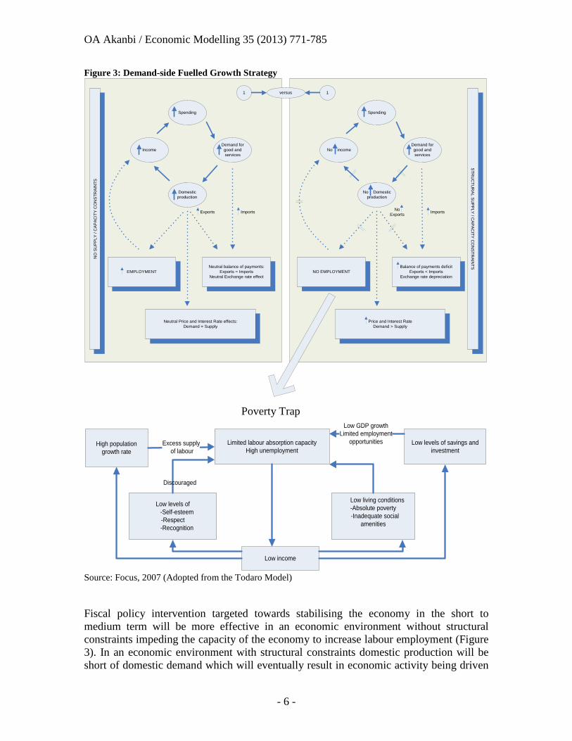
This is achieved by carrying out different fiscal policy simulations on two different economic environments, implying two different model closures in which policy interventions (tax and expenditure changes) may have different economic impacts. These scenarios are presented in Figure 3.


- 6 -

Figure 3: Demand-side Fuelled Growth Strategy

Spending

Domestic production

IncomeDemand for good and services

EMPLOYMENT

Neutral Price and Interest Rate effects: Demand = Supply

Neutral balance of payments: Exports = Imports

Neutral Exchange rate effect

Exports Imports

NO

SU

PPLY

/ C

APAC

ITY

CO

NST

RAI

NTS

Spending

No Domestic production

No incomeDemand for good and services

NO EMPLOYMENT

Price and Interest Rate Demand > Supply

Balance of payments deficitExports < Imports

Exchange rate depreciation

NoExports Imports

STRU

CTU

RAL SU

PPLY / CAPAC

ITY CO

NSTR

AINTS

versus1 1

Poverty Trap

Limited labour absorption capacity High unemployment

Low levels of savings and investment

High population growth rate

Low levels of -Self-esteem

-Respect -Recognition

Low living conditions-Absolute poverty

-Inadequate social amenities

Low income

Excess supply of labour

Low GDP growthLimited employment

opportunities

Discouraged

Source: Focus, 2007 (Adopted from the Todaro Model)

Fiscal policy intervention targeted towards stabilising the economy in the short to medium term will be more effective in an economic environment without structural constraints impeding the capacity of the economy to increase labour employment (Figure 3). In an economic environment with structural constraints domestic production will be short of domestic demand which will eventually result in economic activity being driven


- 7 -

by increased domestic expenditure rather than production and hence will fail to achieve a better income distribution (poverty trap) among the population. On the other hand, fiscal policy actions in an economic environment with no capacity constraints will produce a positive outcome and a better income distribution among the owners of factors of production5.

In this milieu, the study develops two separate models:

Supply-side orientated Model

This represents an economy with structural constraints. In this model gross domestic product (GDP) is estimated in order to detect the constraints that could be impediments to the economic growth and development of the country. In this type of economy a limited capacity to absorb labour in the system results in high and increasing levels of unemployment with depressing socio-economic and growth implications.

Demand-side orientated Model

This represents an economy with limited or no supply constraints. In this model, GDP is generated following the Keynesian identity. In this type of economy, any fiscal policy intervention (tax and expenditure changes) will be more effective on the overall macro economy.

3.2. Methodology and Data This study adopted the Engle and Granger (1987) two-step estimation technique. This procedure is widely accepted in the macro-econometric literature as it avoids the common problem of spurious regressions that give an incorrect impression of an existing long-run relationship between two or more variables.

The models capture both the short-run and long-run dynamic properties of the economy following the procedure laid out in Enders (2004:335). Four sectors of the economy were captured and include the real sector, the external sector, the monetary sector, and the government (public) sector.

Despite its limitation of not being able to control fully for the endogeneity problem that exists among the macro variables, the Engle and Granger technique is still a useful tool in providing various structural relationships among macroeconomic variables. Likewise, its strength in capturing the short-run dynamic properties of the economy cannot be underestimated (Herve et al 2010). The Vector Autoregression (VAR) technique could have served as an alternative approach to correct for these weaknesses, but data limitations have hindered the use of the VAR for this study6.

All the data used in this study were obtained from the South African Reserve Bank (SARB) database, IMF (International Financial Statistics), World Bank database: African Development Indicators and World Development Indicators, and Quantec (Easydata) database. Annual data series which cover the period 1970-2011 were used to estimate the

5 See Akanbi and Du Toit (2011) for a detailed explanation on a demand-side fuelled growth strategy. This idea has been adopted in this study as the general theoretical background. 6 To estimate using VAR, a huge dataset is required for the simultaneous equation model presented in this study given the number of restrictions and lag lengths that may be required on the cointegrating equations and the VAR respectively.


- 8 -

parameters of the model and, where appropriate, the variables were transformed into real figures by using the GDP deflator (2005 = base year).

3.3. Core Structural Equations As mentioned earlier, the study captures both the short-run and long-run dynamic properties of the economy. The long-run core structural equations estimated from the four sectors of the economy are as follows:

3.3.1. The real sector This sector consists of aggregate supply, aggregate demand and a price block. Aggregate supply determines real domestic output by estimating the production function, domestic investment, labour demand, and real wages. Aggregate demand determines aggregate household real consumption expenditure in the economy while the price block estimates producer and consumer prices.

Production function:

the long-run production function is presented as:

),(++

= ttt KNfY (1)

where tY represents output (GDP), tN is the labour employment and tK is the capital stock.

Capital stock

In the model, capital stock is derived through a perpetual inventory method. This means that the current stock of capital is equal to the investment in the current period plus the stock of capital of the previous period, net of depreciation. This is shown as:

ttt IKK +−= −1*)1( δ (2)

where tI is gross domestic investment, and δ is the rate of depreciation which, is about 6.7 per cent on average over the entire period.

Domestic investment (real gross fixed capital formation):

Different approaches, such as the Keynesian model, cash flow model, and the neoclassical model (Jorgenson approach) have been used in modelling investment behaviour. This study considered the neoclassical approach (Jorgenson: 1963) to be the most suitable approach in estimating the domestic investment function because it incorporates all cost minimizing and profit maximizing decision making processes by firms. This approach has also been adopted by Du Toit, 1999; Du Toit and Moolman, 2004; and Pretorius, 1998.

Since there are various components of investment expenditure in the economy, the investment function is divided into two different components: public and private investment. Given this, long-term public investment expenditure will not be affected by any changes in government tax policy. Long-term private investment expenditure will to a larger extent be driven by government tax policy changes.


- 9 -

However, the long-run domestic investment functions are presented below as:

)int,_,_,( ttttP rexchrealratetaxYfIt

−+−−+

= (3)

)int,_,( tttg rexchrealYfIt

−+−+

= (4)

where tgI and

tPI represent public and private investment respectively, tratetax _ is the average tax rate, texchreal _ is the rand/dollar real exchange and tr int is the real interest rate7. Since investment is a long-term phenomenon, the ten-year interest rate on government bonds is used as a measure for cost of capital8.

Labour Demand and Real Wage Determination:

In modelling the labour market, a labour demand equation and a wage adjustment equation are defined and estimated. The long-run labour demand function is presented as:

),(+−

= ttt YrwfN (5) where trw is the real wages.

The real wage equation follows Allen and Nixon (1997:147) and is specified in this study as:

),(−+

= ttt Unemplabprodfrw (6) where tlabprod , is the labour productivity proxy by GDP and tUnemp is the level of unemployment.

Household Real Consumption Expenditure:

The theoretical underpinning of household real consumption expenditure follows the permanent income and life-cycle hypothesis. Therefore, long run household consumption is a function of real disposable income, and real wealth, and this is specified as:

),__(exp_++

= ttt rwealthincdishhfrconhh (7) where trconhh exp_ is household real consumption expenditure, tincdishh __ is household real disposable income, trwealth is real wealth (proxy by real money supply (M3)) (Friedman, 1956; 4-9).

Household real disposable income is however, generated as follows:

)_1(*___ ttt ratetaxhhgdpincdishh −= (8)

Where thhgdp _ is the total household income.

7 For simplicity, the real exchange rate of the rand to the US dollar is adopted in this study since majority of investment expenditure are quoted in US dollar. This has been reflected in the high correlation that exists between the real exchange rate of the rand/dollar and the real effective exchange rate of the rand against its trading partners. 8 Real interest rate is not in its natural logarithms due to negative values in the series.


- 10 -

Consumer and Producer Prices:

The price system helps to achieve a good coordination and communication system in a purely market economy, enabling the various sectors to interact efficiently. This system operates on the principle that everything bought and sold has a price. Through the price system, producers and consumers transmit valuable information to each other, helping to keep the economy in balance.

The production price equation, however, follows Layard and Nickell (1986) and the long-run specification is augmented and presented as:

),,_,(++++

= ttttp

t cuexchpelectwfP (9)

where tw is nominal wages, ptP is production price index, tpelect _ is the electricity

prices (proxy for administered prices), tcu is the capacity utilisation rate and texch is the nominal rand/dollar exchange rate.

Consumer prices, which are directly related to production prices, are also specified as:

),,(+++

= tpt

pt

pt excessdimpPfC (10)

where ptC is the consumer price index, p

timp is the import price on intermediate and consumption goods, and texcessd is excess demand.

To capture fully the effects of imported inflation, an import price is specified following Llewellyn & Pesaran, (1976) and is stated as:

)_,,(+++

= tttpt poilwYexchfimp (11)

where, twY is world (GDP) income in real terms and tpoil _ is the world oil price.

3.3.2. The external sector The external sector identifies the major components of the current account of the balance of payments and the variation in the level of the exchange rate. It estimates the real exports of goods and services, the real imports of goods and services and the rand/ U.S. dollar nominal exchange rate.

Real Exports of Goods and Services:

The demand for real exports of goods and services is in the long run mainly driven by the level of world income and relative prices of goods and services. Fluctuations in the exchange rate are also expected to have an influence in the long run specification of real exports, but depends on the productive structure of that particular economy. The South African real export function is specified as:


- 11 -

)_,(exp++

= ttt exchrealwYfr (12) where tr exp is real exports of goods and services. The real exchange rate is defined as follows:

)/(*_ pt

pustt CCexchexchreal

t= (13)

where pust

C is the consumer price index in the United States.

Real Imports of Goods and Services:

The demand for real imports of goods and services is in the long run mainly driven by the level of domestic income and relative prices of goods and services. Fluctuations in the exchange rate also have a significant impact on the long run specification of real imports since imports dominate a large component of the country’s consumption expenditure. The real imports function is, therefore, specified as:

)_,(−+

= ttt exchrealYfrimp (14)

where trimp is the real imports of goods and services.

Nominal Exchange Rate:

The continued integration of the South African economy into global economic environment has lead to a higher volatility of its exchange rate against major world currencies. These swings have been explained by many other factors not directly mentioned in the conventional Dornbusch (1976, 1980) and Frankel (1979) theory of exchange rate determination. However, in order to capture the long-run nominal exchange equation perfectly, the Frankel, et al (2006) specification was adopted and is presented as:

)__inf,min__,(−+−−

= ttttt priskdifflprealrelYfexch (15) where trelY is relative income (the nominal ratio of domestic GDP to U.S. GDP),

tpreal min__ is the real price of mineral proxy by the real price of gold, tdiffl _inf is the inflation differential between South Africa and the U.S and tprisk _ is the risk premium measured as the difference between prime interest rate and long-term (10-year bond) interest rate.

3.3.3. Monetary sector The essence of modelling the monetary sector in this study is to elicit information regarding the extent to which the monetary variables feed the rest of the economy. The model estimates the money supply (proxy for real wealth) while assuming that the interest rate is exogenously determined by the South African Reserve Bank (SARB). This is done by following the principle that the SARB directly controls interest rates and the monetary policy instrument being used is the interest rate.


- 12 -

Money Supply:

The money supply equation is presented as follows:

),int(+−

= ttt YfRMs (16)

where tRMs is the real money supply, and tint is the nominal prime interest rate.

3.3.4. The government sector In this study, the government sector is assumed to be determined exogenously. The cyclically adjusted fiscal balance analysed in the previous section was used in the model in order to capture fully the structural component of the fiscal policy actions.

Since tax changes have distortionary effects on both households and corporations in the economy, the average tax rate for the entire economy is used as a proxy for both household taxes in the consumption equation and corporate tax in the private investment equation. However, the average tax rate is generated as the ratio of total tax revenue to GDP. Total government expenditure (excluding interest payment) is exogenous in the model and used as one of the tools of fiscal policy actions.

3.4. Structural Equation Diagnostic Properties A detailed exposition of all the data used in the study and their order of integration are carried out and available on request. Table A1 & A2 of Appendix A present the elasticities of the long-run structural equations in the model. Where necessary, dummy variables have been applied to capture any structural breaks (i.e. 1994 transition to democratic dispensation) identified in each specific variables. Cointegration tests were performed in order to detect if there exist long-run relationships among the various variables in each equation. From the visual representation of the residuals presented in Figure A1 of the Appendix, all the structural equations in the model are found to be cointegrated at least at the 10 per cent level.

All the estimated short-run equations with their diagnostic tests (Table A3 & A4) and the long-run simulation paths (Figure A2) of the entire structural equations in the model are also presented in the Appendix. Most of the long-run variables also play an important role in the short-run dynamics. The tables present other variables which do not have any long-run relationship with a particular structural equation but play a significant role in the short-run. The adjustment coefficients are robust (falls between 0 and -1) and statistically significant in bringing back the system to equilibrium.

3.5. Model Closures Model closure reveals the important inter-linkages and feedbacks of the various macroeconomic variables and estimated equations in the system. The type of closure reveals the features of the model developed and how the various policy simulations/scenarios would feed back into the entire system. Therefore, the two models developed in this study are closely based on the following identities:


- 13 -

Supply-side orientated Model

In this model the production function (GDP) is estimated by making the supply-side of the economy more active than the demand-side. Therefore, the price (producer and consumer) equations serve as the link between the demand-side and the supply-side of the economy through excess demand and capacity utilisation. This is presented as:

GDP = ),( KLf

Excess Demand = GDE / GDP, if > 1

GDE = C + I + G

Capacity Utilization = GDP / GDP_POTENTIAL

where L is labour employment, K is capital stock, GDE is gross domestic expenditure, C is household consumption expenditure, I is domestic investment, G is total government expenditure, and GDP_POTENTIAL is the potential level of the GDP.

Demand-side orientated Model

In this model the production function (GDP) is generated by following the Keynesian demand identity, making the demand-side of the economy more active than the supply-side. The price equations remain the linkages between the demand-side and the supply-side of the economy through excess demand and capacity utilisation. This is presented as:

GDP = C + I + G + X – Z

GDE = GDP + Z – X

where X is exports of goods and services, and Z is imports of goods and services. All other identities follow the same way as in the supply-side oriented model.

3.6. Simulation Results: Impact of Fiscal Policy Changes This section provides the simulation results of the effects of fiscal policy actions on major macroeconomic variables in the economy based on the models developed above. The long-run elasticities (relative percentage changes) of the two models are determined and a series of dynamic simulations are carried out by shocking the purely exogenous government expenditure and average tax rate variables in the system to determine the elasticity for every response (endogenous) variable in reaction to the shock variable.

Since one of the main focuses of the study is to detect the most effective way of stabilising the economy using fiscal policy measures, however, the shocks applied are independent of each other. In other words, the effects of fiscal consolidation/expansion are carried out separately when it comes solely from government spending and or solely from taxation.

The elasticities are computed by comparing every response variable’s baseline simulation path with its shocked simulation path. Elasticity is defined as the percentage change in the response variable relative to the percentage of the shock applied. The dynamic elasticities are determined along the simulation path.


- 14 -

The study focuses on the short- to medium-term effects of fiscal policy actions under the assumption that the economy will return to equilibrium at the long-run. In other to make this study relevant to the current global economic situation, fiscal consolidation simulations are carried out and a fiscal consolidation equalling 1 per cent of GDP were applied to the models9. This will directly translate into a 1 per cent increase in the average tax rate when consolidation comes solely from taxation, but this will require about a 4 per cent decrease in government expenditure on the average between 1970 and 2011. Therefore, a positive shock of 1 per cent and negative shock of 4 per cent was applied independently to the average tax rate and government expenditure variables in 1974 respectively10. Every response variable’s simulation path was compared with its baseline path to determine the response elasticities. The process was carried out for the two models developed in the study.

The elasticities of the major response variables for the particular shocks are presented in Figure 4 to 9. Shock results from the two models were compared in order to determine the existing simulation differences. The key objective of the entire process of these models is to observe how effective fiscal policy actions are under the two kinds of economic environments analysed previously and also to detect where consolidation/expansion should come from given the economic environment the country is operating on.

In this milieu, fiscal consolidation typically has contractionary effects on economic activity especially in the short- to medium-term. A fiscal consolidation equivalent to 1 per cent of GDP shows a negative response on the major macroeconomic variables in both economic environments (Figure 4 to 9). This impact is more effective in an economic environment with limited or no supply constraints.

In general, the results revealed that fiscal policy actions that compose more of expenditure changes will be more effective in an economic environment where there is absence of structural supply constraints. Fiscal policy actions that compose more of tax changes will be more effective in an economic environment where there exist huge structural supply constraints.

Since economic activities have been driven by domestic expenditure in a structurally constrained economy, fiscal policy actions through tax changes may have bigger impacts given the distortive effects on household consumption and private investment expenditure. On the other hand, government expenditure changes could be easily constrained through poor governance such as corruption practices, poor regulative framework, government ineffectiveness, and political instability.

9 Note: The effects of a fiscal consolidation would be the reverse of the response to an expansion. 10 The estimated (baseline) model was solved from 1973 due to the lags employed in the short-run equations to capture the deviations from the long-run paths. Therefore, 1973 serves as the year before the consolidation.


- 15 -

Figure 4: Effects on Output of 1% Fiscal Consolidation as a Ratio of GDP

Full government expenditure consolidation (4%)

Full tax consolidation (1%)

Source: Author’s calculations Note: t = 0 denotes the year of the consolidation Figure 5: Effects on Employment of 1% Fiscal Consolidation as a Ratio of GDP



Source: Author’s calculations Note: t = 0 denotes the year of the consolidation


- 16 -

Using full government expenditure consolidation, real output as a result of the shock reduces by about 1 per cent after one year (absence of constraints), with a quick recovery over the next few years11. This shock will only have a minimal negative impact of about -0.1 per cent on output in a constrained economy. Under a full tax consolidation, output fell about 0.16 per cent and 0.32 per cent after one year in an economy with and without structural constraints respectively (Figure 4). A quicker recovery after three years is recorded for the constrained economy while the unconstrained economy’s recovery is slower with some degree of volatility which could be as a result of the short-run direct distortive effect of tax increases on private investment spending. Similar effects of the consolidation are revealed on the level of employment in the country due to the direct link between GDP and employment (Figure 5).

Figure 6: Effects on Domestic Demand of 1% Fiscal Consolidation as a Ratio of GDP




The impact on domestic demand of the shocks will be greater with about 2 per cent reduction after one year in an unconstrained economic environment when consolidation comes fully from spending cuts. In the presence of structural constraints, domestic demand will fall by about 1.5 per cent within one year (Figure 6). Similar simulation paths are recorded within one year of consolidation of about 0.6 per cent in both economic environments, but recovery tends to be faster in the presence of a structural constraint.

11 The simulation results presented in this study is comparable with IMF (2011) simulation path using the Global Integrated Monetary and Fiscal Model (GIMF).


- 17 -

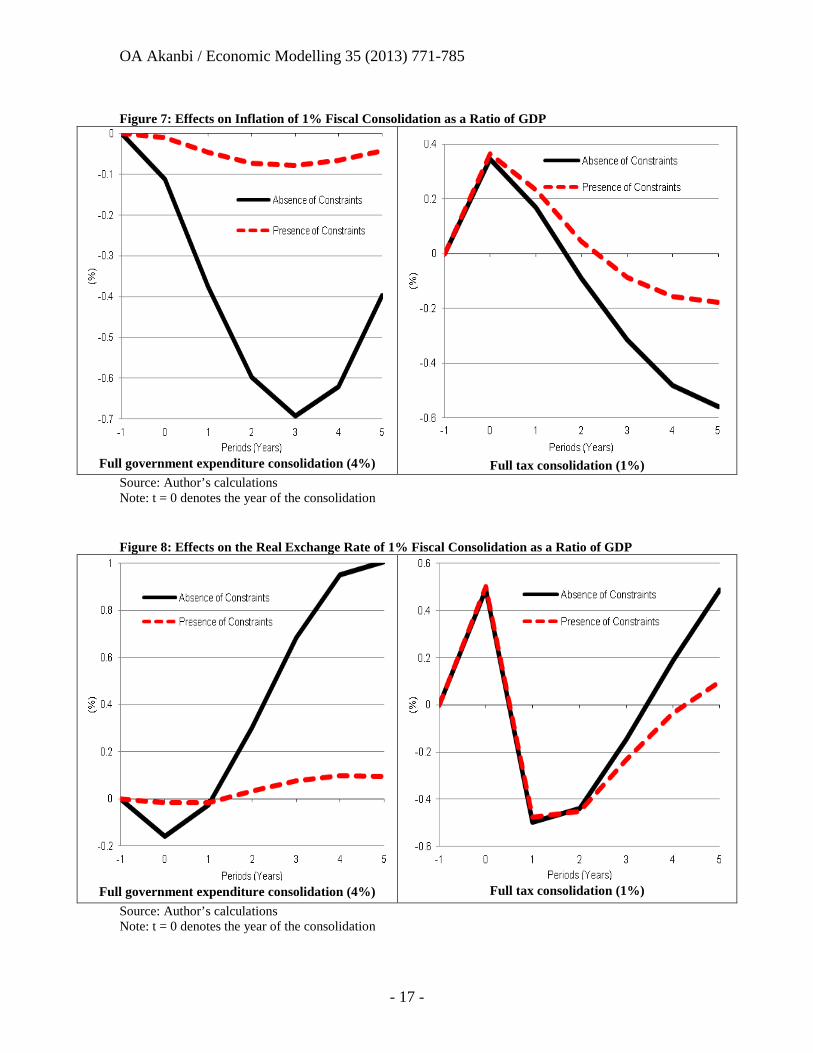
Figure 7: Effects on Inflation of 1% Fiscal Consolidation as a Ratio of GDP



Source: Author’s calculations Note: t = 0 denotes the year of the consolidation Figure 8: Effects on the Real Exchange Rate of 1% Fiscal Consolidation as a Ratio of GDP





- 18 -

With full government expenditure consolidation domestic inflation will fall in both economic environments reaching its lowest after four years. About 0.7 per cent fall is recorded for an unconstrained economy, while about 0.08 percent fall is recorded when there is presence of structural constraints in the system (Figure 7). The extended decline in inflation over the 4-year period can be attributed to the cumulative effects of the fall in excess demand (ratio of domestic demand to GDP) in which government expenditure itself is a component. On the other hand, when consolidation is entirely due to tax increases, domestic inflation tends to rise in the initial first year period by about 0.35 per cent in both economic environments. This rise is attributed to the short-run effect of the tax increases on producer’s prices; thereafter excess demand impact takes over.

The effects on inflation and output are expected to have direct impact on the real exchange rate of the rand to US dollar. A decline in the output differentials in the nominal exchange rate equation is expected to depreciate the currency (rand) while a decline in the inflation differentials should appreciate the currency. However, the net effects of these two variables brought about an appreciation of the rand in the first year when consolidation entirely comprises of spending cuts (Figure 8). This indicates that the impact of the fall in inflation on the value of the currency is greater than the impact of the fall in output. In contrast, a depreciation of the currency is recorded in the first year when consolidation is entirely through tax increases indicating a greater impact of the fall in output than the fall in inflation on the value of the currency.

Figure 9: Effects on the Current Account Balance of 1% Fiscal Consolidation as a Ratio of GDP





- 19 -

The effects of fiscal policy changes on the current account balance are a reflection of how an economy can achieve both internal and external balances. A fiscal consolidation is expected to improve the current account balance through the decline in imports as economic activity declines. But this is also dependent on the effects of the real exchange rate on exports as discussed previously. As shown in Figure 9, the current account balance as a percentage of GDP will deteriorate by about 120 per cent in the first year in an unconstrained economic environment when consolidation is entirely from spending cuts12. In a constrained type of economy, the current account balance will improve as a result of the consolidation by about 2 per cent. These mixed results can be attributed to the fact that, in an unconstrained economy, the magnitude of the fall in exports in the initial year (due to the appreciation of the currency) and the denominator effect of the fall in output outweigh the fall in imports and vice-versa for the constrained economy. However, when consolidation comprises entirely of tax increases, the current account balance tends to perform much better in both types of economic environments. The tendency of the currency (rand) price of imports to rise faster than export prices soon after the depreciation (J-curve effect) has been proven in an unconstrained economic environment.

4. Conclusions and Policy Recommendations This study has analysed the macroeconomic effects of fiscal policy changes in South Africa using explicit and robust macro-econometric models. The historic fiscal performance of the economy identified a counter-cyclicality nature of fiscal policy actions in South Africa over the past four decades. In addition, fiscal policy actions have been largely structural in nature with a slight twist to cyclical trend post apartheid era.

To detect fully the effects of fiscal policy actions on the macro economy, the study deemed it fit to distinguish between two types of economic environments namely: structural supply constrained economy; and limited or no structural supply (demand-side) constrained economy. The models were, however, applied to test the effectiveness of fiscal policy actions in an economy with existing structural supply constraints versus demand-side constraints. It also examine how fiscal consolidation which comprises entirely of tax increases and fiscal consolidation which is entirely from government expenditure cuts will have more painful effects on the macro economy.

The series of dynamic fiscal policy simulations which were performed revealed the importance of the policy analysis of the study. Fiscal policy impacts were derived by shocking the average tax rate and government expenditure variables in the system in order to determine the elasticity for every endogenous variable. A fiscal consolidation equalling 1 per cent of GDP was applied to the system translating into a 1 per cent increase in average tax rate and a 4 per cent cut in government spending.

The results revealed that fiscal policy actions that are composed more of expenditure changes will be more effective in an economic environment where there is absence of structural supply constraints while those that are composed more of tax changes will be

12 Please note that the deterioration in the current account balance do not reflect the actual fall, but rather a deviation from the original path.


- 20 -

more effective in an economic environment where there exist huge structural supply constraints.

Based on the structure of the South African economy and the analysis presented in Section 3.1, the study concludes that the country shows similarities to an environment of structural supply constraints. Therefore, fiscal policy actions may not be exerting their full force in stabilising and projecting the economy on its long-run path to sustainable development.

In order to achieve the optimal objectives of sustained and inclusive economic growth, a well-structured and coordinated policy mix is needed. Policy actions to remove the embedded structural constraints are urgently needed. Such policies are the improvement in governance structures such as the control of corruption, political instability, more effectiveness in government institutions, good regulative framework, presence of rule of law and freedom of speech and accountability. There is also the need to improve substantially on physical infrastructure facilities, the shortage of skills in the economy and meaningful labour market reforms.

Moreover, it is imperative to note the difficulties encountered in analysing fiscal policy actions using a macro-econometric model. The study, however, brought areas that need further investigation to the fore. The major limitation of this study is the unavailability of long-time data, for the adoption of a technique (i.e. VAR-Johansen) that will fully control for the endogeneity problem encountered with the type of simultaneous equation model presented in this study. In addition, the simulation results presented in this study may have taken a different dimension if the different tax components (household and corporate taxes) have been used independently in the model. Future research could however, investigate further the effects of fiscal policy action on the economy, if tax rise or cut should come from household or corporate tax rates. It is also imperative to re-investigate some of the specifications adopted in this study in follow-up studies.


- 21 -

APPENDIX A Table A1: Long-run Elasticities (The Real Sector)

Independent Variables

Dependent Variables

tY tPI tgI tN trw trconhh exp_ p

timp ptP p

tC

tY 1.25 0.9 1.25

tUnemp -0.08

tK 0.7

tN 0.3

trw -0.5

ptP 0.64

tcu 0.78

tlabprod 0.95

tratetax _ -0.62

texchreal _ -0.1 -0.6

tincdishh __ 1.05

tRMs 0.11

tr int -1.28

-3.9

tw 0.34

ptimp 0.36

texcessd 0.16

texch 0.85 0.3

tpoil _ 0.29

tpelect _ 0.29

twY 0.06

Source: Author’s calculations Table A2: Long-run Elasticities (External and Monetary Sector)


Dependent Variables

tr exp trimp texch tRMs

twY 0.73

tdiffl _inf 2.28

tY 0.91 1.31

texchreal _ 0.16 -0.1

trelY -0.43

tpreal min__ -0.42


- 22 -

tprisk _ -0.75

tprime int_ -0.24

Source: Author’s calculations Table A3: Short-run Elasticities (The Real Sector)


Dependent Variables

tY tPI tgI tN trw trconhh exp_ p

timp ptP p

tC

Adjustment coefficients

-0.14

-0.37

-0.12

-0.1 -0.56

-0.55 -0.11 -0.24

-0.06

ptC -

0.19

tprisk _ -0.46

tgovt exp_ 0.89

tratetax _ 0.16

texch -0.07

tpoil _ -0.04

tprime int_ 0.05

Diagnostic Tests Normality 0.36 0.26 0.93 0.12 0.12 0.2 0.95 0.39 0.1 Stability 0.85 0.34 0.5 0.2 0.4 0.23 0.19 0.24 0.78

Heteroscedasticity 0.53 0.38 0.13 0.14 0.1 0.25 0.35 0.25 0.55 Serial correlation 0.35 0.51 0.1 0.16 0.56 0.62 0.51 0.79 0.52 Source: Author’s calculations Note: All diagnostic tests reject the null hypothesis of ‘no normal distribution’, ‘no stability’, ‘heteroscedasticity’, and ‘serial correlation’ at the 10 per cent level of significance. Table A4: Short-run Elasticities (External and Monetary Sector)


Dependent Variables

tr exp trimp texch tRMs Adjustment coefficients

-0.25 -0.3 -0.51 -0.29

tgovt exp_ 0.17

Diagnostic Tests Normality 0.52 0.7 0.36 0.39 Stability 0.2 0.25 0.54 0.84

Heteroscedasticity 0.29 0.21 0.66 0.31 Serial correlation 0.83 0.34 0.1 0.82

Source: Author’s calculations Note: All diagnostic tests rejects the null hypothesis of ‘no normal distribution’, ‘no stability’, ‘heteroscedasticity’, and ‘serial correlation’ at the 10 per cent level of significance.


- 23 -

Figure A1: Long-Run Residuals

-.2

-.1

.0

.1

.2

.3

70 75 80 85 90 95 00 05 10

GDP

-.06

-.04

-.02

.00

.02

.04

.06

70 75 80 85 90 95 00 05 10

HOUSEHOLD_CONSUMPTION

-.15

-.10

-.05

.00

.05

.10

.15

.20

70 75 80 85 90 95 00 05 10

EMPLOYMENT

-.4

-.3

-.2

-.1

.0

.1

.2

.3

70 75 80 85 90 95 00 05 10

INVESTMENT

-.4

-.2

.0

.2

.4

70 75 80 85 90 95 00 05 10

EXPORTS

-.3

-.2

-.1

.0

.1

.2

.3

70 75 80 85 90 95 00 05 10

IMPORTS

-.2

-.1

.0

.1

.2

.3

.4

70 75 80 85 90 95 00 05 10

EXCHANGE_RATE

-.12

-.08

-.04

.00

.04

.08

70 75 80 85 90 95 00 05 10

REAL_WAGES


- 24 -

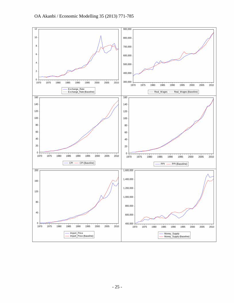
Figure A2: Actual and Estimated (Baseline) Trend Path

600,000

800,000

1,000,000

1,200,000

1,400,000

1,600,000

1,800,000

2,000,000

1970 1975 1980 1985 1990 1995 2000 2005 2010

GDP GDP (Baseline)

400,000

500,000

600,000

700,000

800,000

900,000

1,000,000

1,100,000

1,200,000

1970 1975 1980 1985 1990 1995 2000 2005 2010

household_consumptionhousehold_consumption (Baseline)

2

4

6

8

10

12

14

16

1970 1975 1980 1985 1990 1995 2000 2005 2010

Employment Employment (Baseline)

150,000

200,000

250,000

300,000

350,000

400,000

450,000

1970 1975 1980 1985 1990 1995 2000 2005 2010

Investment Investment (Baseline)

100,000

200,000

300,000

400,000

500,000

600,000

700,000

1970 1975 1980 1985 1990 1995 2000 2005 2010

Exports Exports (Baseline)

100,000

200,000

300,000

400,000

500,000

600,000

700,000

800,000

1970 1975 1980 1985 1990 1995 2000 2005 2010

Imports Imports (Baseline)


- 25 -

0

2

4

6

8

10

12

1970 1975 1980 1985 1990 1995 2000 2005 2010

Exchange_RateExchange_Rate (Baseline)

300,000

400,000

500,000

600,000

700,000

800,000

900,000

1970 1975 1980 1985 1990 1995 2000 2005 2010

Real_Wages Real_Wages (Baseline)

0

20

40

60

80

100

120

140

160

1970 1975 1980 1985 1990 1995 2000 2005 2010

CPI CPI (Baseline)

0

20

40

60

80

100

120

140

160

1970 1975 1980 1985 1990 1995 2000 2005 2010

PPI PPI (Baseline)

0

40

80

120

160

200

1970 1975 1980 1985 1990 1995 2000 2005 2010

Import_PriceImport_Price (Baseline)

400,000

600,000

800,000

1,000,000

1,200,000

1,400,000

1,600,000

1970 1975 1980 1985 1990 1995 2000 2005 2010

Money_SupplyMoney_Supply (Baseline)


- 26 -

REFERENCES

Abbas, S.M., Bouhga-Hagbe, J., Fatas, A.J., Mauro, P. and Velloso, R.C. 2010. Fiscal policy and the current account. IMF Working Paper No. 10/121.

Afonso, A. and Sousa, R.M. 2012. The macroeconomic effects of fiscal policy. Applied Economics, Vol. 44, pp.4439-4454.

Akanbi, O.A. and Du Toit, C.B. 2011. Macro-econometric modelling for the Nigerian economy: a growth-poverty gap analysis. Economic Modelling, Vol.28,pp.335-350.

Allen, C.B., & Nixon, J. 1997. Two Concepts of the NAIRU. In Allen, C.B. and Hall, S.G. (eds), Macroeconomic Modelling in a Changing World: Towards a Common Approach. Chichester: John Wiley and Sons.

BBVA Research. 2012. Spain Economic Outlook. First Quarter. Madrid: BBVA.

Blanchard, O. and Perotti, R. 1999. An empirical characterisation of the dynamic effects of changes of government spending and taxes on output. National Bureau of Economic Research. Working Paper 7269.

Blinder, A.S. and Solow, R.M. 2005. Does fiscal policy matter? In A. Bachi, ed., Readings in Public Finance. New Delhi: Oxford University Press, 283-300.

Calitz, E. 2000. Fiscal implications of the economic globalisation of South Africa. South African Journal of Economics. Vol. 68, No. 4, pp. 564-606.

De Masi, P. 1997. IMF estimates of potential output: theory and practice. Staff Studies for the World Economic Outlook. International Monetary Fund, Washington.

Dornbusch, R. 1976. Expectations and exchange rate dynamics. Journal of Political Economy, Vol.84, No.6, pp.1161-1176.

Dornbusch, R. 1980. Exchange Rate Economics: Where Do We Stand? Brookings Papers on Economic Activity, 1980(1), pp. 143 – 185.

Dornbusch, R.S., Fischer, R. and Starz, R. 1998. Macroeconomic, USA: The McGraw-Hill Companies, Inc.

Du Toit, C.B., & Moolman, E. 2004. A Neoclassical Investment Function of the South African Economy. Economic Modelling, Vol.21, pp.647-660.

Du Toit, C.B. 1999. A Supply-side Model of the South African Economy: Critical Policy Implications. Unpublished Doctoral thesis. Pretoria: University of Pretoria.

Endegnanew, Y, Amo-Yartey, C. and Turn-Jones T. 2012. Fiscal policy and the current account: are microstates different? IMF Working Paper No. 12/51.

Enders W. 2004. Applied Econometric Time Series, 2nd ed. New York: John Wiley and Sons.

Engle, R. & Granger, C. 1987. Cointegration and Error Correction: Representation, Estimation, and Testing. Econometrica, Vol.55,pp.251-76.


- 27 -

Focus, 2007. Integrated social development as the accelerator of shared growth. Compiled by the Bureau for Economic Policy and Analysis (BEPA), Department of Economics, University of Pretoria, no.55.

Frankel, J., Smit, B. and Strurzenegger, F. 2006. South Africa: macroeconomic challenges after a decade of success. Centre for International Development Working Paper No. 133, Harvard University.

Frankel, J.A. 1979. On the Mark: A Theory of Floating Exchange Rates Based on Real Interest Differentials. American Economic Review, Vol. 69, No. 4 (Sep., 1979), pp. 610 – 622.

Friedman, M. 1956. The quantity theory of money: a restatement, in M. Friedman, ed., studies in the Quantity Theory of Money. Chicago: University of Chicago Press.

Gibson, B. and Van Seventer, D. 1997. The macroeconomic impact of restructuring public expenditure by function in South Africa. South African Journal of Economics, Vol. 65, No. 2, pp. 191-223.

Herve, K., Pain, N., Richardson, P., Sedillot, F. and Beffy, P. 2010. The OECD’s new global model. OECD Economics Department Working Papers No. 768, OECD Publishing.

International Monetary Fund. 2011. Separated by birth? The twin budget and trade balances. World Economic Outlook, Chapter 4, September, 2011.

Jorgenson, D. 1963. Capital Theory and Investment Behaviour. American Economic Review, Vol.53, No.2, pp.247-259.

Klein, N. 2011. Measuring the potential output of South Africa. International Monetary Fund, African Department, No. 11/3.

Layard, R. & Nickell, S. 1986. Unemployment in Britain. Economica, Vol.53, pp.S12-S169.

Llewellyn, G.E. and Pesaran, M.H. 1976. The determinants of United Kingdom import prices: a note. The Economic Journal, Vol. 86, No. 342, pp. 315-320.

Ocran, M.K., (2011), “Fiscal Policy and Economic Growth in South Africa”, Journal of Economic Studies, 39 (5), 606-618. Okun, A. 1962. Potential GNP: itsmeasurement and significance. 1962 Proceedings of the Business and Economic Statistics Section of the American Statistical Association, pp.1-7.

Pretorius, C.J. 1998. Gross Fixed Investment in the Macroeconometric Model of the Reserve Bank. Quarterly Bulletin-March 2002 (no.207). Pretoria, South African Reserve Bank.

Ramsey, V. 2008. Identifying government expenditure shocks: It is all in the timing. University of Chicago Mimeo.

Romer, C.D. and Romer, D.H. 2010. The macroeconomic effects of tax changes: estimates based on a new measure of fiscal shocks. American Economic Review, Vol. 100, pp.763-801.


- 28 -

Swanepoel, J.A. and Schoeman, N.J. 2003. Countercyclical fiscal policy in South Africa: role and impact of automatic fiscal stabilizers. South African Journal of Economic and Management Sciences, Vol. 6, No. 4, pp. 802-822.

Documents

Macroeconomic Effects of Fiscal Policy Changes: A Case of