Embed Size (px)
Citation preview
Macroeconomic Regimes∗
Lieven Baele1 Geert Bekaert2 Seonghoon Cho3
Koen Inghelbrecht4 Antonio Moreno5
May 2011
Abstract
We estimate a New-Keynesian macro model accommodating regime-switching behaviorin monetary policy and in macro shocks. Key to our estimation strategy is the use of survey-based expectations for inflation and output. We identify accommodating monetary policybefore 1980, with activist monetary policy prevailing most but not 100% of the time there-after. Systematic monetary policy switched to the activist regime in the 2000-2005 periodthrough an aggressive lowering of interest rates. Discretionary policy spells became less fre-quent since 1985, but the Volcker period is identified as a discretionary period. Outputshocks shift to the low volatility regime around 1985 whereas inflation shocks do so onlyaround 1990, suggesting active monetary policy may have played role in anchoring inflationexpectations. Shocks and policy regimes jointly drive the volatility of the macro variables.We provide new estimates of the onset and demise of the Great Moderation and the relativerole played by macro-shocks and monetary policy.
JEL Classification: E31, E32, E52, E58, C42, C53
Keywords: Monetary Policy, Regime-Switching, Survey Expectations, New-KeynesianModels, Great Moderation, Macroeconomic Volatility, Phillips Curve.
* We appreciate the comments and suggestions of seminar participants at Fordham University andColumbia University.
1 Finance Department, CentER, and Netspar, Tilburg University. Email: [email protected] Graduate School of Business, Columbia University, and NBER. Email: [email protected] School of Economics, Yonsei University. Email: [email protected] Department Financial Economics, Ghent University, and Finance Department, University CollegeGhent. Email: [email protected] Department of Economics, University of Navarra. Email: [email protected]
This is a preprint version of the article. The final version may be found at < http://dx.doi.org/10.1016/j.jmoneco.2014.09.003 >.
Macroeconomic Regimes
May 2011
Abstract
We estimate a New-Keynesian macro model accommodating regime-switching behaviorin monetary policy and in macro shocks. Key to our estimation strategy is the use of survey-based expectations for inflation and output. We identify accommodating monetary policybefore 1980, with activist monetary policy prevailing most but not 100% of the time there-after. Systematic monetary policy switched to the activist regime in the 2000-2005 periodthrough an aggressive lowering of interest rates. Discretionary policy spells became less fre-quent since 1985, but the Volcker period is identified as a discretionary period. Outputshocks shift to the low volatility regime around 1985 whereas inflation shocks do so onlyaround 1990, suggesting active monetary policy may have played role in anchoring inflationexpectations. Shocks and policy regimes jointly drive the volatility of the macro variables.We provide new estimates of the onset and demise of the Great Moderation and the relativerole played by macro-shocks and monetary policy.
JEL Classification: E31, E32, E52, E58, C42, C53
Keywords: Monetary Policy, Regime-Switching, Survey Expectations, New-KeynesianModels, Great Moderation, Macroeconomic Volatility, Phillips Curve.
1 Introduction
The Great Moderation, the reduction in volatility observed in most macro variables since the
mid-1980s, makes it difficult to explain macroeconomic dynamics in the US over the last 40
years within a linear homoskedastic framework. There is still no consensus on whether the
Great Moderation represents a structural break or rather a persistent but temporary change
in regime. The causes also remain the subject of much debate. Was the Great Moderation
the result of a reduction in the volatility of economic shocks, or was it brought about by a
change in the propagation of shocks, for instance through a more aggressive monetary policy?
Articles in favor of the “shock explanation” include McConnell and Perez-Quiros (2000),
Sims and Zha (2006), Liu, Waggoner, and Zha (2010); articles in favor of the policy channel
include Clarida, Galı, and Gertler (1999) and Galı and Gambetti (2008). Nevertheless, there
is empirical evidence of both changes in the variance of economic shocks (Sims and Zha
(2006)) and persistent changes in monetary policy (see Cogley and Sargent (2005), Boivin
(2006), and Lubik and Schorfheide (2004)), necessitating an empirical framework that can
accommodate both.
In this article, we estimate a standard New-Keynesian model accommodating regime
changes in systematic monetary policy, in the variance of discretionary monetary policy
shocks and in the variance of economic shocks. Whereas the model implies the presence of
recurring regimes, it can also produce near permanent changes in regime. With the structural
model, we can revisit the timing of the onset of the Great Moderation, and it so happens, also
its demise. Moreover, we can then trace the sources of changes in the volatility of macroeco-
nomic outcomes to changes in the volatility of demand, supply and discretionary monetary
policy shocks, and to changes in systematic monetary policy. We find that output and in-
flation shocks moved to a lower variability regime in 1985 and 1990, respectively, but move
back to the higher variability regime towards the end of 2008. Systematic monetary policy
became more active after 1980, whereas discretionary monetary policy shocks were much
less frequent after 19851. The aggressive lowering of interest rates in the 2000-2005 period
preceding the recent financial crisis is characterized as an activist regime. Put together, we
identify the 1980-2005 period as a period with substantially lower output and inflation vari-
ability. From several perspectives, including counterfactual analysis, monetary policy was a
critical driver of the Great Moderation.
The estimation of a New-Keynesian (NK) model accommodating regime switches is com-
plicated. In these models, as in most macro models, agents exhibit Rational Expectations,
1Throughout the article we use active or activist policy to indicate the monetary policy regime where theinterest rate reacts to expected inflation more than one to one, in contrast to passive monetary policy.
1
using all the variables, parameters and structure present in the model to form their expect-
ations. While we retain the elegance of the theoretical Rational Expectations model, we
make use of survey forecasts for inflation and GDP in the estimation. Ang, Bekaert, and
Wei (2007) show that survey expectations beat any other model in forecasting future infla-
tion out of sample. The use of survey forecasts not only brings additional information to
bear on a complex estimation problem, but also simplifies the identification of the regimes
under certain assumptions. In the extant literature, survey forecasts have mostly been used
to provide alternative estimates of the Phillips curve (see Roberts (1995) and Adam and
Padula (2003)). Instead, we study the role of survey expectations in shaping macroeconomic
dynamics in the context of a standard NK model, accommodating regime switches.
There are only a handful of DSGE models that incorporate regime-switching and time
variation of structural parameters, including Bikbov and Chernov (2008), Bianchi (2010),
and Fernandez-Villaverde, Guerron-Quintana, and Rubio-Ramırez (2010). These articles use
very different identification strategies, and do not make use of survey expectations. Apart
from our modelling differences, which we discuss further in the model section, our analysis of
the rational expectations equilibrium in a Markov-switching New-Keynesian model extends
Davig and Leeper (2007) to an empirically more realistic setting.
Section 2 describes the New-Keynesian model, detailing the role of regime-switching
and expectations formation. Section 3 discusses the data used and describes the estima-
tion method employed. Section 4 presents the empirical results, emphasizing the parameter
estimates and the identified regimes. Section 5 concludes.
2 The Model
2.1 The basic New-Keynesian model
While our methodology is more generally useful, we focus attention on the following three-
variable-three-equation New-Keynesian macro model, a benchmark of much recent monetary
policy and macroeconomic analysis:
πt = δEtπt+1 + (1− δ)πt−1 + λyt + επ,t, επ,t ∼ N(0, σ2π) (1)
yt = µEtyt+1 + (1− µ)yt−1 − φ(it − Etπt+1) + εy,t, εy,t ∼ N(0, σ2y) (2)
it = ρit−1 + (1− ρ)[βEtπt+1 + γyt] + εi,t, εi,t,∼ N(0, σ2i ) (3)
2
where πt is the inflation rate, yt is the output gap and it is the nominal interest rate.
Et is the conditional expectations operator. The three equations are subject to aggregate
supply (AS), aggregate demand (IS) and monetary policy shocks, respectively. We denote
these shocks by επ,t (AS-shock), εy,t (IS-shock), and εi,t (monetary policy shock). The δ and
µ parameters represent the degree of forward-looking behavior in the AS and IS equation,
respectively, and if they are not equal to one the model features endogenous persistence. The
φ parameter measures the impact of changes in real interest rates on output and λ the effect
of output on inflation. The monetary policy reaction function is a forward-looking Taylor
rule with smoothing parameter ρ. While policy rules featuring contemporaneous rather than
expected inflation are still popular (see e.g. Fernandez-Villaverde, Guerron-Quintana, and
Rubio-Ramırez (2010)), it is well accepted that policy makers consider expected measures of
inflation in their policy decisions (see Bernanke (2010), Boivin and Giannoni (2006)). Policy
should not react to temporary shocks that affect the contemporaneous rate of inflation, but
not the future path of inflation.
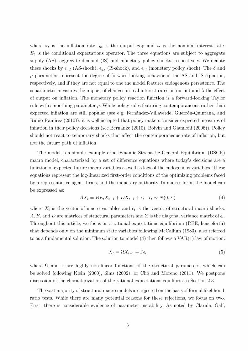
The model is a simple example of a Dynamic Stochastic General Equilibrium (DSGE)
macro model, characterized by a set of difference equations where today’s decisions are a
function of expected future macro variables as well as lags of the endogenous variables. These
equations represent the log-linearized first-order conditions of the optimizing problems faced
by a representative agent, firms, and the monetary authority. In matrix form, the model can
be expressed as:
AXt = BEtXt+1 + DXt−1 + εt εt ∼ N(0, Σ) (4)
where Xt is the vector of macro variables and εt is the vector of structural macro shocks.
A,B, and D are matrices of structural parameters and Σ is the diagonal variance matrix of εt.
Throughout this article, we focus on a rational expectations equilibrium (REE, henceforth)
that depends only on the minimum state variables following McCallum (1983), also referred
to as a fundamental solution. The solution to model (4) then follows a VAR(1) law of motion:
Xt = ΩXt−1 + Γεt (5)
where Ω and Γ are highly non-linear functions of the structural parameters, which can
be solved following Klein (2000), Sims (2002), or Cho and Moreno (2011). We postpone
discussion of the characterization of the rational expectations equilibria to Section 2.3.
The vast majority of structural macro models are rejected on the basis of formal likelihood-
ratio tests. While there are many potential reasons for these rejections, we focus on two.
First, there is considerable evidence of parameter instability. As noted by Clarida, Galı,
3
and Gertler (1999), the monetary authority may have learned over time to react more ag-
gressively to inflation deviations from target in order to tame output and inflation fluc-
tuations, leading to instability in the systematic monetary policy parameters. In addition,
the Great Moderation literature (McConnell and Perez-Quiros (2000), Cogley and Sargent
(2005), Fernandez-Villaverde and Rubio-Ramırez (2007), and Sims and Zha (2006)) shows
that the output shocks identified in both reduced-form and structural models are heteroske-
dastic, displaying a pronounced decline after the mid 1980s. As a result, econometricians have
tried to accommodate these parameter changes through subsample analysis (Clarida, Galı,
and Gertler (1999), Moreno (2004), and Boivin and Giannoni (2006)), time varying struc-
tural parameter and volatility estimation (Kim and Nelson (2006), Fernandez-Villaverde
and Rubio-Ramırez (2007), Ang, Boivin, Dong, and Loo-Kung (2010)) or through regime-
switching models (Bikbov and Chernov (2008) and Sims and Zha (2006)). We incorpor-
ate regime-switching behavior in both systematic monetary policy and the variances of the
structural shocks. The other parameters are assumed time invariant because they arise from
micro-founded models.
Second, the rational expectations assumption may constrain the ability of the current
generation of macro models to characterize macro dynamics. Chief among these shortcom-
ings is the fact that agents only employ the variables used to construct the model in forming
expectations of future macro variables. Given that most macro models only use a limited
number of variables, the information sets used by RE agents seem to be unrealistically con-
strained2. There are a number of potential avenues to overcome this problem. The generalized
method of moments (GMM) allows researchers to condition the estimation of model para-
meters on information sets which include additional variables to those implied by the model
(see, for instance, Clarida, Galı, and Gertler (1999)). Boivin and Giannoni (2008) estimate
a DSGE RE macro model, enhancing the information set available to agents for decision
making purposes with a large number of macro variables governed by a factor structure.
Bekaert, Cho, and Moreno (2010), Bikbov and Chernov (2008), and Rudebusch and Wu
(2008) use term structure data to help identify a New-Keynesian macro model. The work of
Bikbov and Chernov (2008) is most closely related to ours, as they also allow regime shifts in
2Moreover, RE imply that all agents have a perfect knowledge of the model and only adjust their ex-pectations in reaction to the model dynamics in order to reach the equilibrium, leaving no room for anyalternative perceptions or mechanisms which in practice would likely alter their decisions. According to So-low (2004) and Phelps (2007), this tight endogeneity of the RE framework may impair its ability to explainmacro dynamics. On the theoretical side, De Grauwe (2008) develops a DSGE model where agents exhibitbounded rationality, whereas Sims (2005) introduces the rational inattention concept, relaxing some of theRE assumptions. In addition, Onatski and Stock (2002), among others, develop techniques to perform policyanalysis in the presence of model, parameter and shock uncertainty around a reference model, thus leavingsome room for macro realizations to deviate from a benchmark model with perfectly known parameters andforcing processes.
4
the shock variances and systematic monetary policy. However, their identification strategy is
very different, as they use term structure data and an exogenous pricing kernel (inconsistent
with the IS curve) to price the term structure.
Instead, we use survey-based expectations (SBE) to help identify the parameters of a
DSGE macro model. SBE reflect the direct answers of a large number of economic agents
to questions about the expected future path of macroeconomic variables. Unlike RE, SBE
are thus not model conditioned and naturally reflect the different perceptions of economic
agents based on a potentially very rich information set. Recently, several authors (Roberts
(1995), Adam and Padula (2003) and Nunes (2007)) have estimated New-Keynesian Phillips
curves using SBE. The results of these efforts have overall been positive, as the estimate of the
important Phillips curve parameter, linking inflation to the output gap, becomes statistically
significant under SBE, in contrast to the results produced by most RE models. Nevertheless,
the use of SBE in DSGE macro models has been limited to date and restricted to single-
equation estimation. Of course, there is much skepticism about SBE: agents may not be truth-
telling or may omit important information in forming forecasts of future macro variables.
However, Ang, Bekaert, and Wei (2007) show that SBE of inflation predict inflation out-
of-sample better than a large number of the standard structural and reduced-form inflation
models proposed in the literature3. Consequently, SBE likely contain important information
about future macro variables. We show below that incorporating SBE greatly facilitates the
computation of the likelihood function and thus the identification of the regime shifts.
2.2 Introducing regime switches
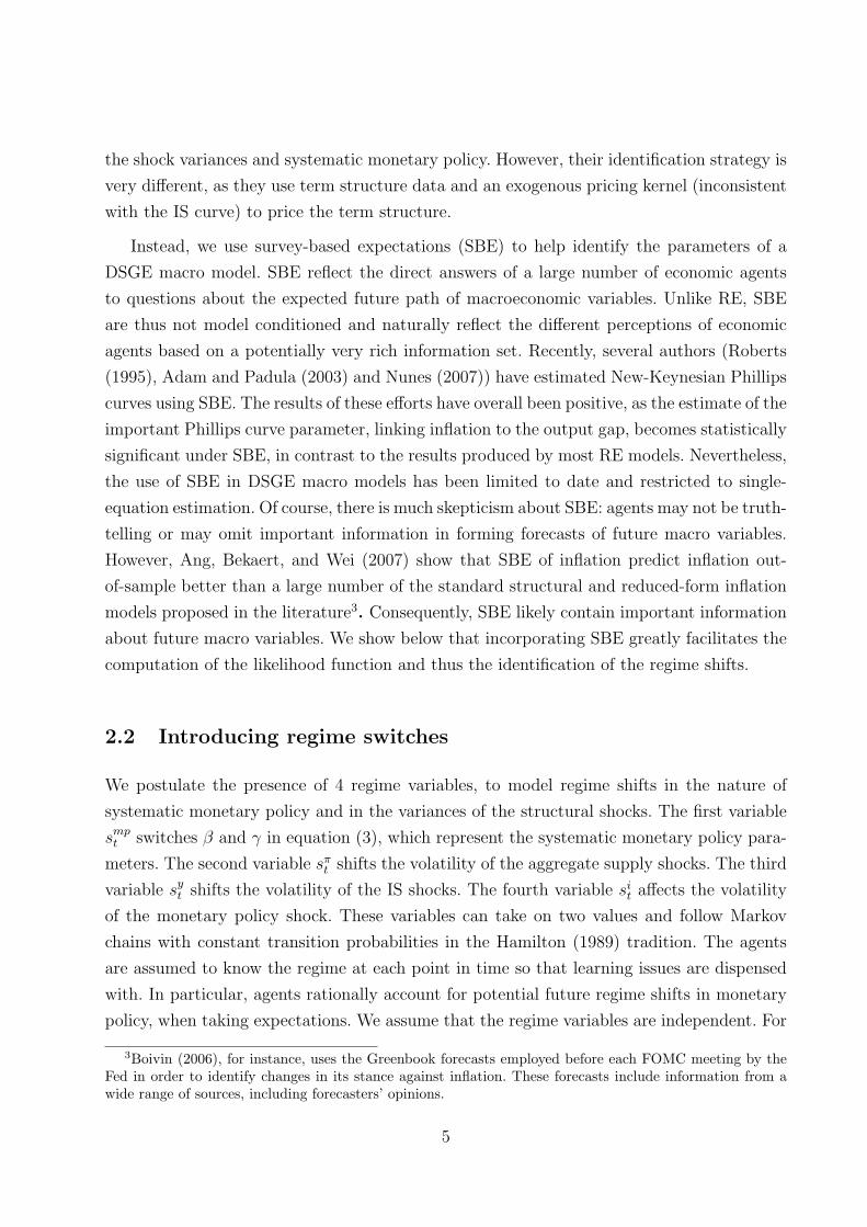
We postulate the presence of 4 regime variables, to model regime shifts in the nature of
systematic monetary policy and in the variances of the structural shocks. The first variable
smpt switches β and γ in equation (3), which represent the systematic monetary policy para-
meters. The second variable sπt shifts the volatility of the aggregate supply shocks. The third
variable syt shifts the volatility of the IS shocks. The fourth variable si
t affects the volatility
of the monetary policy shock. These variables can take on two values and follow Markov
chains with constant transition probabilities in the Hamilton (1989) tradition. The agents
are assumed to know the regime at each point in time so that learning issues are dispensed
with. In particular, agents rationally account for potential future regime shifts in monetary
policy, when taking expectations. We assume that the regime variables are independent. For
3Boivin (2006), for instance, uses the Greenbook forecasts employed before each FOMC meeting by theFed in order to identify changes in its stance against inflation. These forecasts include information from awide range of sources, including forecasters’ opinions.
5
future reference, let St = (smpt , sπ
t , syt , s
it).
The regime-dependent volatility model for the three shocks in equation (4) simply allows
for two different values of the conditional variance, as a function of the regime variable. For
example, for the AS equation, we have:
V ar (επ,t|Xt−1, St) = σ2π (sπ
t ) = exp (απ,0 + απ,1sπt ) (6)
with sπt = 1, 2 and the exponential function guaranteeing non-negative volatilities. To help
identification, we impose σ2π (sπ
t = 1) > σ2π (sπ
t = 2) , σ2y (sy
t = 1) > σ2y (sy
t = 2) , σ2i (si
t = 1) >
σ2i (si
t = 2).
The regime variable smpt accommodates potential persistent shifts in the systematic policy
parameters β and γ. In particular, we expect to find an activist regime with β larger than
1 and a passive regime with β smaller than 1. A number of economists (Clarida, Galı, and
Gertler (1999), Boivin and Giannoni (2006)) suggest that β experienced a structural break
around 1980, with β being lower than 1 before and larger thereafter. While we find such
a model ex ante implausible, it can still be approximated by our regime-switching model
if the regimes are very persistent with very small transition probabilities. Nevertheless, in
our model, a switch to a new regime is never viewed as permanent. If regime classification
yields a passive regime 100% of the time before 1980, and an activist regime 100% of the
time afterwards, the permanent break hypothesis surely gains credence relative to a model
of persistent but non-permanent changes in policy. It is also possible that the influential
1979-1982 Volcker period affects inference substantially. Was this period the first switch
into a more active regime or is it best viewed as a period of discretionary contractionary
policy? By letting the variable sit affect the variability of the monetary policy shock, we also
accommodate the latter possibility.
Incorporating the regime variables, equation (4) becomes:
A(St)Xt = B(St)EtXt+1 + DXt−1 + εt εt ∼ N(0, Σ(St)) (7)
where A(St) and B(St) capture the regime-switching behavior of the central bank and Σ(St)
governs the time-varying volatilities of the structural shocks. With regimes affecting both
systematic monetary policy and the variance of shocks, we can use the model to revisit the
question of what drove down inflation and output growth variability during the 1980s and
1990s: was it policy or luck (see e.g. Stock and Watson (2002) and Blanchard and Simon
(2001))? A large literature has examined this issue from both reduced-form (Cogley and
Sargent (2005), McConnell and Perez-Quiros (2000), Sims and Zha (2006)) and structural
6
(Moreno (2004), Lubik and Schorfheide (2004), Boivin and Giannoni (2006)) perspectives.
Disagreement remains. For instance, Benati and Surico (2009) show that the results of Sims
and Zha (2006), suggesting a prominent role for heteroskedasticity, may be biased against
finding a role for policy changes. The combination of a structural New-Keynesian model
with regime shifts in both monetary policy parameters and shock variables can provide
novel evidence on the sources of macroeconomic dynamics.
Our model fits into a rapidly growing body of work incorporating policy changes and/or
heteroskedasticity into New-Keynesian models. Part of this literature is more theoretical
in nature, considering issues of equilibrium existence and stability, in models that are not
likely to be empirically successful. We discuss this important literature in Section 2.3. The
empirical literature on DSGEs with time-varying parameter and shock distribution is very
recent. Some authors, such as Fernandez-Villaverde and Rubio-Ramırez (2007) and Justini-
ano and Primiceri (2008), postulate heteroskedastic variances and fixed structural paramet-
ers in their DSGEs, whereas Davig and Doh (2008) develop a New-Keynesian model with
regime-switching parameters but constant shock variances. Fernandez-Villaverde, Guerron-
Quintana, and Rubio-Ramırez (2010), Bianchi (2010) and Bikbov and Chernov (2008) allow
for time variation in both the structural shock variances and the systematic part of their RE
New-Keynesian macro models, and are thus closest to our framework. Bianchi (2010) has
a three equation - three variable model, such as ours, but uses only one regime variable to
accommodate heteroskedasticity. We show below that this is overly restrictive. Our use of
SBE also allows for a much simpler estimation method than is possible in Bianchi (2010).
2.3 The rational expectations equilibrium under regime-switching
A linear rational expectations model (4) is said to be determinate if it has a unique and
stable (non-explosive) equilibrium, which takes the form of a fundamental REE as in equa-
tion (5). In case of indeterminacy, the models generally have multiple fundamental and
non-fundamental (“sunspot”) equilibria. It is also now well-understood that a violation of
the Taylor principle, typically identified as β being less than 1 in equation (3), leads to
indeterminate equilibria in the prototypical New-Keynesian model. Intuitively, raising the
short-term nominal interest rate less than one for one to an increase in (expected) inflation
actually lowers the real rate, fueling inflation even more through output gap expansion and
the Phillips curve mechanism. However, the US data seem to suggest a structural break in
β, with β lower than 1 (“passive policy’) before 1980 and higher than 1 (“active policy”)
afterwards (Clarida, Galı, and Gertler (1999), Boivin and Giannoni (2006)). From the per-
spective of a standard New-Keynesian model, this implies that the propagation system was
7
not uniquely determined before 1980 and/or that non-fundamental (sunspot) equilibria may
have played a role before 1980 (see Lubik and Schorfheide (2004)).
Recently, Davig and Leeper (2007) generalized the Taylor principle to a baseline New-
Keynesian macro model with regime-switching in monetary policy, which is nested in the
model of equation (7). Specifically, they show that the model can have a unique bounded
equilibrium even when the central bank is temporarily passive as long as there is a positive
probability that the passive regime switches to the active regime, and the structural shocks
are bounded. Consequently, a Markov-switching rational expectations model (MSRE for
short), apart from being more economically reasonable than a permanent break model, offers
the potential to explain US macro-dynamics, even before 1980, in the context of a model
with a unique and stable equilibrium.
It should be stressed that determinacy for MSRE models has not been completely char-
acterized. The debate between Davig and Leeper (2007) and Farmer, Waggoner, and Zha
(2009), for example, shows that standard determinacy conditions do not always easily gen-
eralize to MSRE models. The main reason is that, in contrast to linear models, boundedness
in mean and boundedness in variance represent different stability concepts in MSRE mod-
els. Moreover, the extant work on determinacy does not apply to our model, as our model
features predetermined variables, which are absent in the MSRE models analyzed thus far
in the literature.
Instead, our approach circumvents this debate by focusing on the “forward solution,”
introduced by Cho and Moreno (2011). In a nutshell, the forward solution results from
solving a linear RE model recursively forward. If a forward solution exists, the parameters
multiplying the state variables converge, and hence, the recursion also yields the actual fun-
damental equilibrium. Cho and Moreno (2011) show that the forward solution is the unique
fundamental solution that satisfies the no-bubble (or transversality) condition; the condition
that makes expectations of future endogenous variables converge to zero. Consequently, the
forward solution selects an economically reasonable fundamental equilibrium, irrespective
of determinacy and delivers the numerical solution in one step. Importantly, Cho (2010)
shows that this logic carries over to MSRE models. In particular, the forward solution to the
Markov-switching model (7) follows the law of motion:
Xt = Ω(St)Xt−1 + Γ(St)εt εt ∼ N(0, Σ(St)), (8)
which depends only on the state variables, Xt−1 and the current state St in a nonlinear
fashion. Hence, there are as many “different” reduced-form solutions as there are combina-
tions of regimes. This is the methodology we follow to both compute and select the REE for
8
our model. Consequently, our analysis excludes non-fundamental equilibrium solutions and
fundamental solutions that violate the transversality condition.
Because REE in MSRE models as general as ours have not been examined before (and
to aid our practical estimation), we conducted an extensive study of the existence of REE
for different parameter configurations. The analysis is described in more detail in Appendix
A, but we provide a short summary of the major findings here. Essentially, we conduct a
grid search over an extensive parameter range, and verify whether we can characterize the
set of parameters for which a fundamental forward solution exists. This proved a non-trivial
task and no simple characterization is possible. However, the most critical parameters in
driving the existence of a REE clearly are (δ, µ, β1, β2). Recall that β1 > β2, identifying
the first regime as the “active” regime. Not surprisingly, given Davig and Leeper’s work, an
equilibrium can still exist with β2 smaller than 1, and β1 larger than 1. Values of µ and δ
smaller than 0.5 will lead to non-existence, but equilibrium may exist if only one of the two
is smaller than 0.5 (and the other one relatively high).
We use this information to consider a restricted parameter space in estimation (see more
below). Nevertheless, estimating the model in Equations (7)-(8) remains difficult. In order
to construct the likelihood function, we must not only integrate across all combinations of
potential (unobserved) regimes, but also numerically compute the highly non-linear reduced-
form coefficient matrices (Ω(St) and Γ(St)) for all combinations of potential regimes. We
circumvent this problem and simultaneously bring additional information to bear on the
estimation by incorporating survey forecasts, as we show in the next subsection.
2.4 Introducing survey expectations
Undoubtedly, the information used by professional forecasters greatly exceeds the informa-
tion set spanned by the variables present in the simple model in equations (1)-(3). Given
that survey expectations outperform empirical and theoretical models predicting inflation,
they can also prove useful in estimating macroeconomic parameters and dynamics. To in-
corporate SBE into the model, we assume that survey expectations of inflation and output
obey the following law of motion:
πft = αEtπt+1 + (1− α)πf
t−1 + wπt (9)
yft = αEtyt+1 + (1− α)yf
t−1 + wyt (10)
with wπt ∼ N
(0, σπ
f
)and wy
t ∼ N(0, σy
f
). Consequently, survey expectations potentially
react to true rational expectations one for one if α equals 1, but may also slowly adjust to
9
true rational expectations and depend on past survey expectations. This is reminiscent of
Mankiw and Reis (2002)’s model of the Phillips curve, in which information disseminates
slowly throughout the population.
In our model, we combine the determination of SBE with the regime-switching counter-
parts of equations (1)-(3). That is, we retain the assumption of rational expectations, and
simply use additional information to identify both the structural parameters and the regimes
in a 5 variable system. Nevertheless, the estimation remains complex as we still need to solve
the rational expectations equilibrium at each step in the optimization and for all possible
regime combinations. If we let the variance of the shocks in equations (9)-(10) go to zero,
so that SBE are an exact function of past SBE and current RE, we can greatly simplify
estimation. In this case, we can infer the RE of inflation and output from equations (9) and
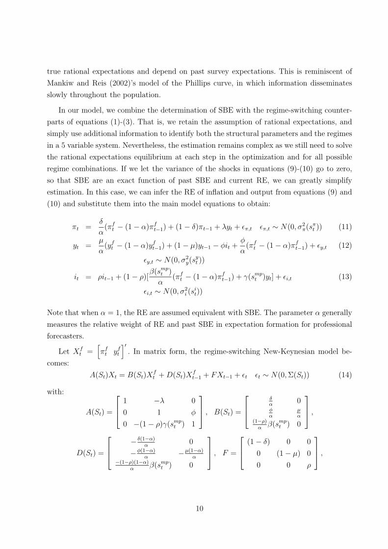
(10) and substitute them into the main model equations to obtain:
πt =δ
α(πf
t − (1− α)πft−1) + (1− δ)πt−1 + λyt + επ,t επ,t ∼ N(0, σ2
π(sπt )) (11)
yt =µ
α(yf
t − (1− α)yft−1) + (1− µ)yt−1 − φit +
φ
α(πf
t − (1− α)πft−1) + εy,t (12)
εy,t ∼ N(0, σ2y(s
yt ))
it = ρit−1 + (1− ρ)[β(smp
t )
α(πf
t − (1− α)πft−1) + γ(smp
t )yt] + εi,t (13)
εi,t ∼ N(0, σ2i (s
it))
Note that when α = 1, the RE are assumed equivalent with SBE. The parameter α generally
measures the relative weight of RE and past SBE in expectation formation for professional
forecasters.
Let Xft =
[πf
t yft
]′. In matrix form, the regime-switching New-Keynesian model be-
comes:
A(St)Xt = B(St)Xft + D(St)X
ft−1 + FXt−1 + εt εt ∼ N(0, Σ(St)) (14)
with:
A(St) =
1 −λ 0
0 1 φ
0 −(1− ρ)γ(smpt ) 1
, B(St) =
δα
0φα
µα
(1−ρ)α
β(smpt ) 0
,
D(St) =
− δ(1−α)α
0
−φ(1−α)α
−µ(1−α)α
−(1−ρ)(1−α)α
β(smpt ) 0
, F =
(1− δ) 0 0
0 (1− µ) 0
0 0 ρ
,
10
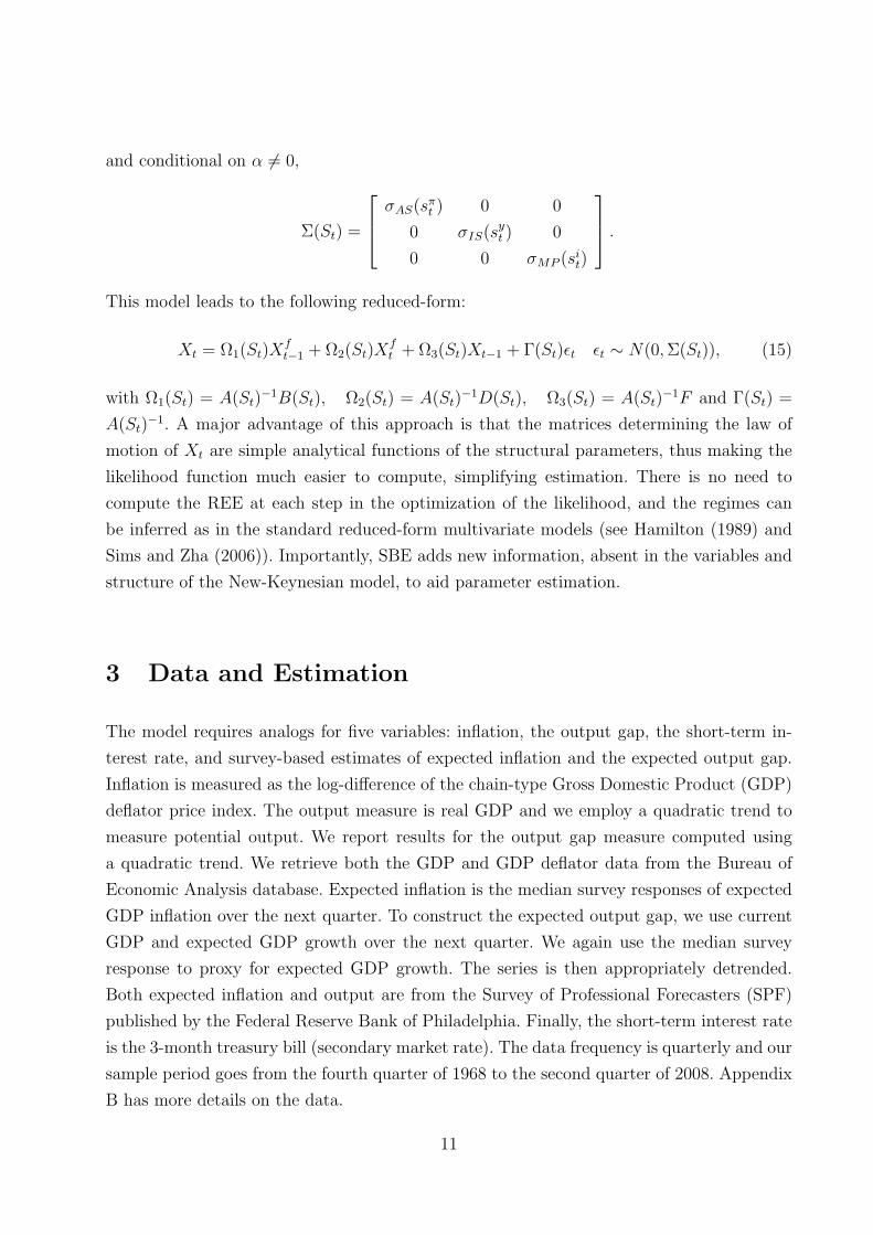
and conditional on α 6= 0,
Σ(St) =
σAS(sπt ) 0 0
0 σIS(syt ) 0
0 0 σMP (sit)
.
This model leads to the following reduced-form:
Xt = Ω1(St)Xft−1 + Ω2(St)X
ft + Ω3(St)Xt−1 + Γ(St)εt εt ∼ N(0, Σ(St)), (15)
with Ω1(St) = A(St)−1B(St), Ω2(St) = A(St)
−1D(St), Ω3(St) = A(St)−1F and Γ(St) =
A(St)−1. A major advantage of this approach is that the matrices determining the law of
motion of Xt are simple analytical functions of the structural parameters, thus making the
likelihood function much easier to compute, simplifying estimation. There is no need to
compute the REE at each step in the optimization of the likelihood, and the regimes can
be inferred as in the standard reduced-form multivariate models (see Hamilton (1989) and
Sims and Zha (2006)). Importantly, SBE adds new information, absent in the variables and
structure of the New-Keynesian model, to aid parameter estimation.
3 Data and Estimation
The model requires analogs for five variables: inflation, the output gap, the short-term in-
terest rate, and survey-based estimates of expected inflation and the expected output gap.
Inflation is measured as the log-difference of the chain-type Gross Domestic Product (GDP)
deflator price index. The output measure is real GDP and we employ a quadratic trend to
measure potential output. We report results for the output gap measure computed using
a quadratic trend. We retrieve both the GDP and GDP deflator data from the Bureau of
Economic Analysis database. Expected inflation is the median survey responses of expected
GDP inflation over the next quarter. To construct the expected output gap, we use current
GDP and expected GDP growth over the next quarter. We again use the median survey
response to proxy for expected GDP growth. The series is then appropriately detrended.
Both expected inflation and output are from the Survey of Professional Forecasters (SPF)
published by the Federal Reserve Bank of Philadelphia. Finally, the short-term interest rate
is the 3-month treasury bill (secondary market rate). The data frequency is quarterly and our
sample period goes from the fourth quarter of 1968 to the second quarter of 2008. Appendix
B has more details on the data.
11
The model in (15) is estimated via limited information maximum likelihood, given that
we do not use the πft and yf
t equations. The information set It−1 consists of all the available
information up to time t − 1: It−1 = Qt−1, Qt−2, . . . , Q0, where Qt = [Xt Xft ]′.
The full dataset is thus QT = [QT , QT−1, . . . , Q0]. We denote the parameters to be
estimated as θ, so that the aim is to maximize the density function f(QT ; θ). While agents in
the economy observe the regime variables, St, the econometrician does not and only has data
on Qt. Therefore, we maximize the likelihood function for QT , integrating out the dependence
on St, as is typical in the regime-switching literature4.
We would like the estimation to produce parameters for which a fundamental rational
expectations equilibrium exists. To do so, we proceed in two steps. First, we use the analysis
of Section 2.3 to construct a compact parameter space that attempts to exclude regions
where REE are unlikely to exist. Because of the non-convexity of the set, we use a rather
wide parameter space (details are available upon request), that encompasses the parameter
values yielding a REE. Second, at each step in the optimization, we verify whether the
forward solution exists. If not, the likelihood function is penalized, steering optimization
away from such regions in the parameter space.
Appendix C describes the different specification tests that we perform on the residuals
of the model. First, for each equation, we test the hypotheses of a zero mean and zero
serial correlation (up to two lags) of the residuals (the “mean test”); unit mean and zero
serial correlation (two lags) for the squared standardized residuals (the “variance test”);
zero skewness, and appropriate kurtosis. In performing these tests, we recognize that the
test statistics may be biased in small samples, especially if the data generating process is as
non-linear as the model is above. Therefore, we use critical values from a small Monte Carlo
analysis also described in Appendix C. Second, the economic model should also capture
the correlation between the various variables. We test for each residual whether its joint
covariances with all other residuals are indeed zero. We also perform a joint test for all
covariances. As in the first set of tests, we obtain critical values from a small Monte Carlo
analysis.
Table 1 reports Monte Carlo p-values of all these tests for our main model, on the left
hand side. The residual levels and variances are well behaved, with the exception of the
output gap, where the test uncovers some remaining autocorrelation in the residuals. The
regime-switching model is able to capture most skewness and kurtosis in the data, only
failing the zero skewness test for inflation. The model’s weakest point appears to be the fit
4We sacrifice full efficiency by ignoring f(Xft |It−1; θ) in the estimation. Technically, this requires assuming
f(Xft |St = st, It−1; θ) = f(Xf
t |It−1; θ). While not very palatable at first, in our model, the regimes can inprinciple be identified without using survey data, so that the assumption is implicitly valid.
12

of covariances between the three shocks. The last two lines in Table 1 reveal that the model
fails to fully capture the correlation structure between the various economic variables.
4 Empirical Results
4.1 Parameter estimates
Table 2 presents the parameter estimates of the RS DSGE New-Keynesian macro model
yielding a stable and determinate RE equilibrium, as described in Section 2.3. It also shows
a number of statistical tests of parameter equality. All parameters have the right sign and
are statistically significant, but we did constrain the φ coefficient to a positive value of 0.1.
As is common in maximum likelihood estimation of this class of New-Keynesian models,
unconstrained estimation yields either negative or very small and insignificant estimates of
φ (see Ireland (2001), Fuhrer and Rudebusch (2004) and Cho and Moreno (2006)).
In the AS equation, δ is 0.425, implying a similar weight on the forward-looking and
endogenous persistence terms. The IS equation is more forward looking, since µ is 0.675.
Given the small standard errors of these parameters, our estimation reveals strong evidence
in favor of endogenous persistence.
The Phillips curve parameter λ is large at 0.102, implying a strong transmission mech-
anism from output to inflation and thus a strong monetary policy transmission mechanism.
Previous estimations of rational expectations models fail to obtain reasonable and significant
estimates of λ with quarterly data (Fuhrer and Moore (1995)). Some alternative estimations
have yielded significant estimates, such as Galı and Gertler (1999) who use a measure for
marginal cost replacing the output gap; Bekaert, Cho, and Moreno (2010) who identify a
natural rate of output process from term structure data; or Roberts (1995) and Adam and
Padula (2003) who use SBE but in a single equation context with fixed regimes. However,
our estimate is even larger than the coefficients reported in these articles. We conjecture that
the introduction of slow moving SBE of inflation generates additional correlation between
(expected) inflation and the output gap.
Regarding the monetary policy rule, the interest rate persistence is large, 0.834, in agree-
ment with most studies in the literature (Clarida, Galı and Gertler (1999), Bekaert, Cho
and Moreno (2010), among others). Our estimation allows for regime switches in the key
monetary policy parameters, β, the response to expected inflation, and γ, the response to
the output gap. In the “activist” regime, β is 2.312, well above 1 statistically, whereas in
the passive regime, β is 0.598, significantly below 1. Thus, our estimation clearly identifies a
13

sharp economic and statistical difference in the response to inflation across monetary policy
regimes. In their single equation monetary policy rule estimation, Davig and Leeper (2005)
also estimate a significant difference between β’s across regimes, but of a smaller magnitude
than our estimates. The contemporaneous articles of Bikbov and Chernov (2008) and Bi-
anchi (2010), estimating Markov Switching RE New-Keynesian models, also identify a large
difference in β across regimes. The interest rate response to the output gap, γ, is higher
than in the aforementioned estimations (1.187 and 0.687, respectively), and it is larger in
the more “activist” regime, although not in a statistically significant way.
Finally, α, the parameter governing the law of motion for the survey-based expectations,
is 0.986, meaning that SBE adjust almost completely to RE. We examine below whether
this finding is the result of imposing rational expectations on the estimation. Because the
other parameters are directly related to the identification of the regimes, we discuss them in
the next sub-section.
4.2 Macroeconomic regimes
Perhaps the key output of our model is the identification of macroeconomic regimes. The
volatility parameters imply strong evidence of time-varying variances in macroeconomic
shocks. For the output gap and inflation shocks, volatility in the high volatility regime is
around double that in the low volatility regime. However, for interest rates, the high volat-
ility regime features volatility that is about 6 times as high as in quiet times, suggesting
a potentially important role for discretionary monetary policy. Because interest rates are
measured in quarterly percent, the volatility of interest rate shocks in the low volatility state
is very small (0.04%), implying a strict commitment to the monetary policy rule.
The transition probability coefficients imply overall quite persistent regimes. For inflation,
the expected duration of the high variance regime is very high at 100 quarters, but the low
variance regime is persistent as well. Output gap regimes are somewhat less persistent, with
the high variance regime expected to last about 27 quarters, while discretionary interest rate
regimes are much less persistent, with the high interest rate variability regime expected to
last about 8 quarters. Accommodating monetary policy regimes last on average longer than
activist regimes, which are short-lived lasting on average 7 quarters.
These transition probabilities are important inputs in the identification of the time path
of the regimes. Figure 1 plots the smoothed probabilities for the four independent regime
variables. Panel A shows the smoothed probabilities of respectively the high inflation shock
volatility regime and the high output shock volatility regime. Note that the regime probab-
14
ilities tend to be either close to one or zero, indicating adequate regime identification. We
observe a sudden drop in output shock volatility starting in 1981 and fully materializing
in 1985. The decreased volatility persists until 2007, coinciding with the onset of the credit
crisis. The variability of inflation shocks starts to decrease later, with the smoothed prob-
ability going below 0.5 at the beginning of 1986, and going toward zero just before the 1990
recession. Signs of a reversal in the low variability regime are already visible in 2003, with its
probability reaching less than 50 percent in the third quarter of 2006 already. Our evidence
in favor of a switch towards a higher variability regime is stronger and its timing earlier than
in Bikbov and Chernov (2008).
Panel B shows the smoothed probabilities of respectively the active monetary policy
regime in which the Fed aggressively stabilizes inflation, and the high volatility regime for
interest rate shocks. The high interest rate volatility regime occurs quite frequently and is
always on during recessions, including during the 1980-1982 Volcker period. This implies that
in times of recession, the Fed is more willing to deviate from the interest rate rule. Bikbov
and Chernov (2008) also categorize the Volcker period as a period of discretionary monetary
policy. Unlike their results, we also find systematic monetary policy to be activist during this
period. Interestingly, our model shows that activist monetary policy spells generally became
more frequent from 1980 onwards. We identify the 1993-2000 period as an accommodating
monetary policy stance. Because this period is characterized by relatively low inflation, a
passive monetary policy stance implies relatively high interest rates. One interpretation is
that inflation expectations were firmly anchored, due to the more aggressive stance of the Fed
during the previous decade. In addition, the possibility of switching back to the stabilizing
regime, as captured by our regime switching DSGE, may also anchor inflation expectations.
Notice that this regime identification is quite different from the permanent shift in monetary
policy around 1980, put forward in earlier studies such as Clarida, Galı, and Gertler (1999)
and Lubik and Schorfheide (2004), but consistent with contemporaneous results in Bianchi
(2010) and Fernandez-Villaverde, Guerron-Quintana, and Rubio-Ramırez (2010).
In 2000 there is a switch to the activist regime, as interest rates rapidly declined following
the beginning of the 2000 recession, while inflation stayed low. Hence, according to our
analysis, interest rates in the first 5 years of the previous decade were lower than what
was prescribed by the Taylor rule (see Taylor (2009)). Bernanke (2010) ascribes this to
the “jobless recovery” experienced at the time, but some may surmise that this aggressive
monetary policy was one of the root causes of the recent credit crisis (see Rajan (2006)). The
recent credit crisis starting in 2007 is preceded by a passive monetary policy regime which,
given the low inflation environment, implies that interest rates increased. In the beginning
of the credit crunch, our model identifies a switch towards both systematic stabilizing and
15
(expansionary) discretionary monetary policy, leading to a sharp decline of interest rates.
4.3 Impulse responses
A nice feature of our model is that the impulse responses are regime-dependent, and should
differ across regimes. Because agents are assumed to know the regime, we compute the
impulse responses using an information set that incorporates both data and the regime;
they follow from calculating E [Xt+k|It, smpt = i], for i = 1, 2. Appendix D describes a simple
procedure to compute these impulse responses recursively. Note that this computation takes
into account the expectations of agents regarding future switches in the monetary policy
regime.
Figures 2 to 4 produce these regime dependent impulse responses of all three macro-
variables to one-standard deviation shocks, focusing on, respectively, AS, IS and monet-
ary policy shocks. In each figure, there are three panels corresponding to the three macro-
variables. We show 4 different impulse responses, depending on the monetary policy regime
and the shock volatility regime. While the volatility regimes only affect the initial size of
the shock, the relative magnitude of the impulse responses helps us interpret macroeconomic
dynamics in different time periods.
Figure 2 focuses on AS shocks. This is of considerable interest as there is a lively debate
on whether the stagflations of the seventies were partially policy driven. The figure shows
that following an AS shock, inflation is highest in the high volatility passive monetary policy
regime, as was observed in the 1970s, and lowest in the low volatility-activist monetary policy
regime, as observed throughout the 90s. It is especially activist monetary policy that contrib-
utes to a lower inflation response. Investigating output gap responses, a positive AS shock
drives down the output gap in a protracted way under an activist monetary policy response,
because the real interest rate increases. However, the output gap increases when monetary
policy is accommodating as then the real interest rate decreases following a positive AS
shock. However, after about 6-7 quarters, the output gap is lower under an accommodating
regime than it is under an activist regime. The effect of AS shocks on nominal interest rates
is also strikingly regime-dependent. Except for the initial periods, the accommodating re-
gime yields higher nominal interest rate responses than the activist regime. This is because
under accommodating monetary policy, it takes time for inflation to decrease - both through
the direct effect of monetary policy and through expectations -, so that interest rates must
be kept high for a long time. The regime-dependent responses therefore provide simultan-
eously an interesting interpretation of the historical record on the macroeconomic response
16
to the negative aggregate supply shocks in the seventies and a counter-factual analysis. The
accommodating policy regime implied (excessively) high interest rates, high inflation and
high inflation variability and a substantial long term loss in output. The responses under an
activist regime show that an aggressive Fed could have likely lowered the magnitude of the
inflation response, reduced inflation volatility, kept interest rates overall lower and avoided
the longer-term output loss, at the cost of a short-term loss over the first 5 quarters.
Figure 3 shows the responses to the IS shock. The inflation responses are similar across
monetary policy regimes, but move over a wider range under the accommodating regime.
In that regime, inflation rates move substantially below their mean during some periods,
simultaneously with the interest rate undershooting its mean. The output gap responses
are also quite similar across regimes. The similarity of the responses may have something
to do with the fact that monetary policy reacts similarly to demand shocks across both
regimes. While Panel C shows that the interest response to a demand shock is higher in
the activist regime, the response differences are both in absolute and relative terms multiple
times smaller than the responses to supply shocks, observed in Figure 2.
Finally, Figure 4 shows the responses to the monetary policy shock. Clearly, the activist
monetary policy regime implies (much) more stable inflation and output dynamics than the
passive regime. The macroeconomic volatility under the accommodating regime is especially
dramatic when the interest rate shock is in the high volatility regime (recall that the interest
rate shock volatility is multiple times higher in that case). A contractionary monetary policy
shock lowers inflation and the output gap in both regimes, but, as the third panel shows,
this is not only accommodated with less macroeconomic but also less interest rate volatility
in the activist regime.
4.4 Macro-variability and its Sources
US economic history has witnessed profound changes in the volatility of macroeconomic
variables over time, as evidenced by the literature on the Great Moderation. In the context of
our model, this time variation in macroeconomic variability is driven by changing regimes in
the variability of macroeconomic shocks (driven by sπt , sy
t , sit) and regime dependent feedback
parameters, which also depend on the monetary policy regime, smpt . In this section, we
derive the unconditional and regime–dependent variances of our macro variables, and provide
different decompositions to shed light on the sources of macroeconomic variability.
17
4.4.1 A Variance Decomposition
The regime variable St contains 16 different regimes, as each of the four independent re-
gimes, smpt , sπ
t , syt and si
t has two states. Appendix E shows in detail how to compute the
unconditional variance as a sum of regime-dependent variances:
V ar(Xt) =S∑
i=1
V ar(Xt|St = i) · Pi (16)
where Pi = Pr(St = i) is the unconditional, ergodic regime probability, and S = 16. Appendix
E also derives closed-form expressions for the regime-dependent variances. We then compute
the contribution of a particular regime of a particular regime to the total variance as:
rx(St = i) =V ar(xt|St = i)Pi
V ar(xt)(17)
where xt represents πt, yt or it.
Table 3 reports these ratios together with the long run, ergodic distribution (Pi). For
instance, the regime combination of an active monetary policy and high shock volatility
across all three equations contributes 1.24, 1.98 and 3.17% to the total variance of inflation,
the output gap and the interest rate, respectively. The regimes contributing the most to
the unconditional variance reflect passive monetary policy, the high variability regime for
inflation shocks and the low variability regime for output shocks. The latter is true because
the low variability regime for output occurs more frequently than the high variability regime
(69.81% versus 30.19% in fact), whereas the opposite is true for inflation shocks, where the
high variability regime occurs 68.97% of the time and also for interest rate shocks where the
high variability regime occurs 59.47% of the time.
The most noticeable result is that in all cases, the contribution to total variance of any
variable is much smaller under the active monetary regime than it is under the passive
regime. For instance, when the economy is in the high volatility regime for all shocks, the
active regime contributes only 1.98% to the total variance of the output gap, whereas the
passive regime contributes 14.31%, about 7.23 times more. Of course, the contribution could
simply be low because the active regime has a much lower probability of occurring. In the
high volatility regimes, the ergodic probability of the active regime is 3.23% while it is
9.16% under the passive regime, about three times higher. Therefore, even after controlling
for differences in ergodic probabilities, the volatility of the output gap under the active
regime is much smaller than that under the passive regime. This is generally true for all
18

regime combinations and all the macro-variables.
To see this more explicitly, Table 4 shows variance ratios for the various regimes, that is
the variance in that particular regime relative to the unconditional variance. Strikingly, the
variance ratios for output and inflation variability in the active regime when all the shocks
are in the high variability regime is lower than the variance ratio for the output and inflation
variability in the passive regime when all the shocks are in the low variability regime. This
suggests that the monetary policy regime has a rather important impact on macro-variability
and perhaps an impact that exceeds the impact of the variability of macro shocks.
To compare the relative effect on variability of shocks versus policy, the last line shows
the ratio of the variance in a regime where all macro shocks are in the high variability regime
versus the variance of a regime where all the macro shocks are in the low variability regime.
These ratios obviously depend on the macro variable and the policy regime, but their range
is rather narrow varying between 3.09 and 3.71. To compare this to the effect of monetary
policy, Table 5 shows the ratio of the passive versus active variances, controlling for the
shock variability regimes. It is obvious that policy has a relatively larger effect on output
and inflation variances than do macro shocks. In terms of volatilities (standard deviations),
the passive monetary policy regime leads to macro standard deviations that are about two
to three times as large as macro standard deviations in the active regime.
4.4.2 The Great Moderation
The above computations can also help us identify the start and the end of the Great Mod-
eration. In terms of our covariance stationary model, the Great Moderation is a period in
which the regime-dependent variance is substantially below its unconditional counterpart.
Figure 5 graphs the ratio of an estimate of the regime-dependent variance over time relative
to the unconditional variance for inflation, the output gap and interest rates. To estimate
regime dependent variances, we use the smoothed regime probabilities. That is,
V ar[Xt|IT ] =S∑
i=1
V ar[Xt|St = i]P [St = i|IT ] (18)
If regime classification is perfect (that is, the smoothed probabilities are zero or 1), the
summation simply selects one of the 16 regime-dependent variances. Visually, the graph
clearly identifies the Great Moderation lasting from the third quarter of 1980 to the third
quarter of 2004, with inflation and output variability being substantially below the 1 line,
often even being less than 50% of the unconditional variance. Do note that there are short
19
episodes during the Great Moderation where inflation and particularly output variability
briefly spike up.
Our previous computations suggest that policy played a rather important role in the
Great Moderation. For example, it is striking that we identify the Great Moderation to start
before the shock variabilities move to a higher variability regime. This is, of course, due to a
switch from a passive to active monetary policy regime around 1980. To visualize the effect of
policy on macro-variances, we run a counterfactual analysis. In Figure 6, we graph a volatility
ratio, namely the volatility of the three macro variables, conditional on the monetary policy
regime always being in the passive regime versus the unconditional volatility. That is, when
computing the counterfactual volatility, the underlying variances computation transfers mass
from states where Smpt = 1 to the corresponding state (and its variance) where Smp
t = 2.
Figure 7 does the opposite computation, it computes the volatility assuming the monetary
policy regime is always activist, and graphs the actual over the activist volatility.
With these two graphs in hand, we can reinterpret the historical evolution of macro-
volatility as generated by our model. In the seventies, macro-volatility was around twice
as high as it could have been, had monetary policy been active (see Figure 7). From 1981
to 1993, active monetary policy managed to reduce macro-volatility substantially - it would
have been 50% to 200% higher otherwise (Figure 6). The relatively subdued macro-variability
after 1993 to around 2000 was due to low variability in the macro shocks, as monetary policy
was passive. Of course, as we have argued before, the earlier aggressive policy stance may
have helped anchor expectations during a rather mild macroeconomic climate. Taking our
model literally, monetary policy could have further reduced macro-volatility by continuing
to be aggressive. Because inflation was low at that time, an active monetary policy would
have meant lower interest rates. The jump in counterfactual volatility around 2000 in Figure
6 is the more dramatic of the two graphs. In other words, if monetary policy had remained
passive, macro-volatilities would have increased substantially. Bernanke’s (2010) speech ex-
plicitly discusses this episode as the Federal Reserve reacting aggressively to a deflation scare,
reducing the interest rate way below what a standard Taylor rule would predict. The period
also witnessed a number of macroeconomic shocks that could have caused macro-volatility
to increase and augmented recession risk, such as the events of September 11, 2001.
4.5 Robustness checks
To ensure that our results are robust, we consider a few alternative specifications. We sum-
marize some major features of these alternative estimations in Table 6, repeating the main
20
estimation results in the left column. The first two estimations we consider simply put φ
equal to a different number than the current value of 0.10, namely 0.01 and 0.20. The Phil-
lips curve parameter, λ, remains large in both cases, and the stark contrast between the
expected inflation response parameters in the active and passive monetary policy regimes
is preserved. We also report the start and end of the Great Moderation for the variability
of both output and inflation shocks under the various models. For output, the end of the
low volatility regime is always in the first or second quarter of 2008, but the alternative
estimations time the beginning of the low output shock volatility regime a bit later than
our main estimation did. For inflation, using a smaller φ gives very similar results to the
main estimation, but using φ = 0.20 delays the start of the low volatility regime from the
second quarter of 1986 to the second quarter of 1990, and speeds up its demise by three
quarters (from the third quarter in 2006 to the last one in 2005). Do note that our cut-off for
regime classification is 0.5: that is, as soon the shock volatility regime has a larger than 50%
smoothed probability of being in either regime it is classified as being in that regime. How-
ever, when inflation transitions to a lower volatility regime, the regime probabilities in the
models for φ = 0.10 and φ = 0.01 hover around 0.5 for a while, meaning that classification
is uncertain. When we use a more stringent classification of the probability being in either
regime being 70%, the start of the low inflation shock volatility regime is in early 1990 in
all three cases. Finally, the last two rows report the probability of activist spells before and
after 1980. For all three model specifications we find no activist spells before 1980 and an
elevated occurrence of activist spells post 1980.
The second set of columns report the three previous estimations but making γ regime
invariant. The results are very robust, with the remarks about the start of the Great Mod-
eration for inflation shocks being the same as before.
4.6 Rational expectations versus survey expectations
Our estimation imposes a parameter space that ensures the existence of a fundamental
rational expectations equilibrium. What happens if this assumption is relaxed? Table 7
shows the results for the unconstrained estimation. In Table 1, the right-hand side panel
also produces specification tests for this model. The model only performs marginally better
than the constrained model. Moreover, the resulting estimates imply explosive dynamics for
the RE model. Nevertheless, it is noteworthy that the parameter estimates are very similar
to those obtained in the constrained estimation. The only significant difference is that µ, the
forward-looking parameter in the IS equation, is now significantly smaller, 0.331, relative
to 0.675 before. This is similar to the values obtained by Fuhrer and Rudebusch (2004),
21
in their systematic single equation estimation in a fixed regime context. Bekaert, Cho, and
Moreno (2010) also estimate a lower value for µ, namely 0.422, but this is coupled with
a high estimate for the degree of forward-looking behavior in the AS equation (δ in our
model). As we have verified through simulation exercises, the combination of low δ and low
µ –maintaining standard values for other parameters - implies the non-existence of a stable
RE equilibrium, both in a fixed regime and in a multiple regime context. In economic terms,
stable RE dynamics require AS and IS equations with a sufficient degree of forward looking
behavior, such that shocks are rapidly absorbed.
Finally, α, the parameter governing the law of motion for the survey-based expectations,
is 0.410 in the unconstrained case, whereas it was 0.986 in the constrained estimation. This
is an important difference. When we enforce a stable RE, RE appear indistinguishable from
SBE, whereas in the unconstrained estimation, SBE slowly adjust to RE, being heavily in-
fluenced by past expectations. In fact, α is statistically indistinguishable from 0.5, implying
that rational expectations and past survey-based expectations obtain similar relative weights
in the expectations formation process. In other words, viewed through the lens of this mac-
roeconomic model, survey expectations only slowly adjust to rational expectations, being
heavily influenced by past expectations. This is consistent with Mankiw, Reis, and Wolfers
(2003), who show that the adjustment of SBE to the macro environment is gradual. Con-
versely, the dependence on rational expectations is highly significant, implying that survey
expectations likely convey much information, useful in estimating macroeconomic parameters
and dynamics.
Figure 8 shows the regime probabilities for the unconstrained model, which should be
compared to Figure 1 for the RE model. Focusing first on Panel B, the monetary policy regime
identification, both for systematic and discretionary policy is very similar, qualitatively and
quantitatively, to that in the constrained estimation. In Panel A, we observe some differences
in terms of output shock regime identification. First, the high output volatility prevails
from the beginning of the sample, whereas in the unconstrained estimation this regime
appears more gradually. In addition, the Great Moderation in terms of output volatility
shocks starts abruptly around 1986, which is a few years later than in the constrained
estimation. Second, the low volatility output shock regime already ends in 2000, much earlier
than in the constrained optimization. These differences can be easily understood examining
the transition probabilities of the IS shock regime variable across estimations (see Tables
2 and 6). The unconstrained estimation shows much more persistence in the high variance
regime and less persistence in the low volatility regime than the constrained estimation.
22
5 Conclusions
In this article, we identified macroeconomic regimes through the lens of a simple New-
Keynesian model accommodating regime switches in macroeconomic shocks and systematic
monetary policy. We demonstrate that monetary policy has witnessed several spells of activist
policy, which have become more frequent post 1980. Nevertheless, we do not see a permanent
switch from accommodating to activist policy around 1980, but rather occasional switches
back and forth between the two regimes. One reason is that the data suggest an important
and time-varying role for discretionary monetary policy. For example, the Volcker period
is characterized by both activist systematic policy and discretionary active policy. We also
document important changes in the variances of output and volatility shocks. It is no surprise
that we find strong evidence of a “shock variability moderation” occurring around 1985 for
output, whereas for inflation the timing is somewhere between 1985 and 1990. What is new
is that we find strong evidence of this volatility reduction having ended, for output at the
onset of the recent economic crisis (more precisely in 2007), for inflation, earlier in 2005. The
variability of shocks is not the only determinant of macro-variability however. Our model
implies that the effect of monetary policy regimes on macro variability is relatively larger
than the effect of the variability of shocks. When we investigate the time path of the overall
variability of inflation and the output gap, we find that the Great Moderation starts around
1980 and ends in about 2005. During that period, a predominantly active monetary policy
and low variability economic shocks combined to make output and inflation substantially
less variable than unconditional averages would suggest.
Estimating a rational expectations New-Keynesian model with regime switches is very
difficult from a numerical perspective. Our innovation was to expand the information set
with survey expectations on inflation and output growth. By formulating a simple law of
motion for these expectations as a function of the true rational expectations, we could greatly
simplify the likelihood construction. Constraining the parameter space to those parameters
that yield a stable rational expectations equilibrium, we find survey expectations to be
almost equivalent to rational expectations. However, when we relax these constraints, we
find survey expectations to only gradually adjust to rational expectations and the parameters
to be outside the rational expectations equilibrium space. Fortunately, the identification of
regimes remains similar to that obtained in the rational expectations model, except that the
Great Moderation in terms of output volatility ends much earlier (in 2000!) when identified
from the unconstrained model.
There are two possible interpretations to these different estimation results. One possib-
ility is that agents truly have rational expectations but that our New-Keynesian model is
23

mis-specified. Perhaps, we need a more intricate natural rate of output process or we must
add investment equations as in Smets and Wouters (2007) to better fit the data. We did
experiment with slightly more complex specifications (e.g. three monetary policy regimes,
state-dependent transition probabilities, correlated regimes) within the confines of the styl-
ized New-Keynesian model, finding little improvement in fit, and no noteworthy new results.
Perhaps some of the parameters we now assume to be time-invariant may also be unstable.
Hofmann, Peersman, and Straub (2010), for instance, indicate that the degree of wage in-
dexation may vary through time, causing instability in the AS equation. An alternative
possibility is that the assumption of rational expectations is too rigid, and we must build a
model that accommodates the presence of agents with not fully rational expectations. In any
case, we hope this article stimulates the use of survey expectations in building and estimating
macroeconomic models.
References
Adam, K., and M. Padula, 2003, “Inflation Dynamics and Subjective Expectations in the
United States,” ECB Working Paper, No. 222.
Ang, A., G. Bekaert, and M. Wei, 2007, “Do Macro Variables, Asset Markets or Surveys
Forecast Inflation Better?,” Journal of Monetary Economics, 54, 1163–1212.
Ang, A., G. Bekaert, and M. Wei, 2008, “The term structure of real rates and expected
inflation,” The Journal of Finance, 63(2), 797–849.
Ang, A., J. Boivin, S. Dong, and R. Loo-Kung, 2010, “Monetary Policy Shifts and the Term
Structure,” Review of Economic Studies, Forthcoming.
Bekaert, G., S. Cho, and A. Moreno, 2010, “New-Keynesian Macroeconomics and the Term
Structure,” Journal of Money, Credit, and Banking, 42(1), 33–62.
Benati, L., and P. Surico, 2009, “VAR Analysis and the Great Moderation,” American Eco-
nomic Review, 99, 1636–52.
Bernanke, B., 2010, “Monetary Policy and the Housing Bubble,” Speech at the Annual Meet-
ing of the American Economic Association, Atlanta (Georgia).
Bianchi, F., 2010, “Regime Switches, Agent’s Beliefs, and Post-World War II U.S.,” Duke
University Working Paper.
24
Bikbov, R., and M. Chernov, 2008, “Monetary Policy Regimes and The Term Structure of
Interest Rates,” Working Paper, Columbia University.
Blanchard, O., and J. Simon, 2001, “The long and large decline in US output volatility,”
Brookings Papers on Economic Activity, (1), 135–174.
Boivin, J., 2006, “Has US Monetary Policy Changed? Evidence from Drifting Coefficients
and Real-Time Data,” Journal of Money, Credit and Banking, 38(5), 1149–1173.
Boivin, J., and M. P. Giannoni, 2006, “Has Monetary Policy Become More Effective?,”
Review of Economics and Statistics, 88(3), 445–462.
, 2008, “Optimal Monetary Policy in a Data-Rich Environment,” Working Paper.
Cho, S., 2010, “Characterizing Markov-Switching Rational Expectations Models,” Working
Paper.
Cho, S., and A. Moreno, 2006, “A Small-Sample Study of the New-Keynesian Macro Model,”
Journal of Money, Credit and Banking, 38(6), 1461–1482.
, 2011, “The Forward Method as a Solution Refinement in Rational Expectations
Models,” Journal of Economic Dynamics and Control, 35(3), 257–27.
Clarida, R., J. Galı, and M. Gertler, 1999, “The science of monetary policy: A New Keynesian
perspective,” Journal of Economic Literature, 37(4), 1661–1707.
Cogley, T., and T. J. Sargent, 2005, “Drifts and volatilities: monetary policies and outcomes
in the post WWII US,” Review of Economic Dynamics, 8(2), 262–302.
Davig, T. A., and T. Doh, 2008, “Changes in Inflation Persistence: Lessons from Estimated
Markov-Switching New Keynesian Models,” Federal Reserve Bank of Kansas City, mimeo.
Davig, T. A., and E. M. Leeper, 2005, “Fluctuating Macro Policies and the Fiscal Theory,”
Federal Reserve Bank of Kansas-City, mimeo.
, 2007, “Generalizing the Taylor Principle,” American Economic Review, 97(3), 607–
635.
De Grauwe, P., 2008, “DSGE-Modelling when Agents are Imperfectly Informed,” ECB Work-
ing Paper, No.897.
Farmer, R. E., D. F. Waggoner, and T. Zha, 2009, “Understanding Markov-switching rational
expectations models,” Journal of Economic Theory, 144(5), 1849–1867.
25

Fernandez-Villaverde, J., P. Guerron-Quintana, and J. Rubio-Ramırez, 2010, “Fortune or
Virtue: Time-Variant Volatilities Versus Parameter Drifting in U.S. Data,” University of
Pennsylvania Working Paper.
Fernandez-Villaverde, J., and J. F. Rubio-Ramırez, 2007, “Estimating macroeconomic mod-
els: A likelihood approach,” Review of Economic Studies, 74(4), 1059–1087.
Fuhrer, J. C., and G. Moore, 1995, “Inflation Persistence,” Quarterly Journal of Economics,
440, 127159.
Fuhrer, J. C., and G. Rudebusch, 2004, “Estimating the Euler Equation for Output,” Journal
of Monetary Economics, 51, 1133–1153.
Galı, J., and L. Gambetti, 2008, “On the Sources of the Great Moderation,” American
Economic Journal: Macroeconomics, 1(1), 26–57.
Galı, J., and M. Gertler, 1999, “Inflation dynamics: A structural econometric analysis,”
Journal of Monetary Economics, 44(2), 195–222.
Hamilton, J. D., 1989, “A New Approach to the Economic Analysis of Nonstationary Time
Series and the Business Cycle,” Econometrica, 57(2), 357–384.
Hofmann, B., G. Peersman, and R. Straub, 2010, “Time Variation in U.S. Wage Dynamics,”
European Central Bank Working Paper No. 1230.
Ireland, P., 2001, “Sticky-Price Models of the Business Cycle: Specification and Stability,”
Journal of Monetary Economics, 47, 318.
Justiniano, A., and G. Primiceri, 2008, “The Time Varying Volatility of Macroeconomic
Fluctuations,” American Economic Review, Forthcoming, 98(3), 604641.
Kim, C.-J., and C. R. Nelson, 2006, “Estimation of a forward-looking monetary policy rule:
A time-varying parameter model using ex post data,” Journal of Monetary Economics,
53(8), 1949–1966.
Klein, P., 2000, “Using the generalized Schur form to solve a multivariate linear rational
expectations model,” Journal of Economic Dynamics and Control, 24(10), 1405–1423.
Liu, Z., D. F. Waggoner, and T. Zha, 2010, “Sources of Macroeconomic Fluctuations: A
Regime-Switching DSGE Approach,” Working Paper.
Lubik, T., and F. Schorfheide, 2004, “Testing for Indeterminacy: An Application to U.S.
Monetary Policy,” American Economic Review, 94(1), 190–217.
26
Mankiw, G., R. Reis, and J. Wolfers, 2003, “Disagreement about Inflation Expectations,”
NBER Working Paper No 9796.
Mankiw, N. G., and R. Reis, 2002, “Sticky information versus sticky prices: A proposal
to replace the new Keynesian Phillips curve,” Quarterly Journal of Economics, 117(4),
1295–1328.
McCallum, B. T., 1983, “On non-uniqueness in rational expectations models: An attempt
at perspective,” Journal of Monetary Economics, 11(2), 139–168.
McConnell, M. M., and G. Perez-Quiros, 2000, “Output fluctuations in the United States:
What has changed since the early 1980’s?,” American Economic Review, 90(5), 1464–1476.
Moreno, A., 2004, “Reaching Inflation Stability,” Journal of Money, Credit, and Banking,
36(4), 801–825.
Newey, W. K., and K. D. West, 1987, “A simple, positive semidefinite, heteroskedasticity
and autocorrelation consistent covariance-matrix,” Econometrica, 55(3), 703–708, 15.
Nunes, R., 2007, “Inflation Dynamics: The Role of Expectations,” Mimeo, Board of Gov-
ernors of the Federal Reserve.
Onatski, A., and J. H. Stock, 2002, “Robust monetary policy under model uncertainty in a
small model of the US economy,” Macroeconomic Dynamics, 6(1), 85–110.
Phelps, E. S., 2007, “Macroeconomics for a modern economy,” American Economic Review,
97(3), 543–561.
Rajan, R. G., 2006, “Has Finance Made the World Riskier?,” European Financial Manage-
ment, 12, 499–533.
Roberts, J. M., 1995, “New Keynesian economics and the Phillips curve,” Journal of Money
Credit and Banking, 27(4), 975–984.
Rudebusch, G., and T. Wu, 2008, “A Macro-Finance Model of the Term Structure, Monetary
Policy, and the Economy,” Economic Journal, 118, 906–926.
Sims, C., 2002, “Solving Linear Rational Expectations Models,” Computational Economics,
20(1-2).
Sims, C., 2005, “Rational Inattention: A Research Agenda,” Deutsche Bundesbank Discus-
sion Paper no. 34/2005.
27
Sims, C. A., and T. Zha, 2006, “Were there regime switches in US monetary policy?,”
American Economic Review, 96(1), 54–81.
Smets, F., and R. Wouters, 2007, “Shocks and Frictions in US Business Cycles: A Bayesian
DSGE Approach,” American Economic Review, 97(3), 586–606.
Solow, R. M., 2004, “Introduction: The Tobin approach to monetary economics,” Journal of
Money Credit and Banking, 36(4), 657–663.
Stock, J. H., and M. W. Watson, 2002, “Has the business cycle changed and why?,” NBER
Macroeconomic Annual 2002, 17, 159–218.
Taylor, J. B., 2009, “The Financial Crisis and the Policy Responses: An Empirical Analysis
of What Went Wrong,” NBER Working Paper 14631.
28
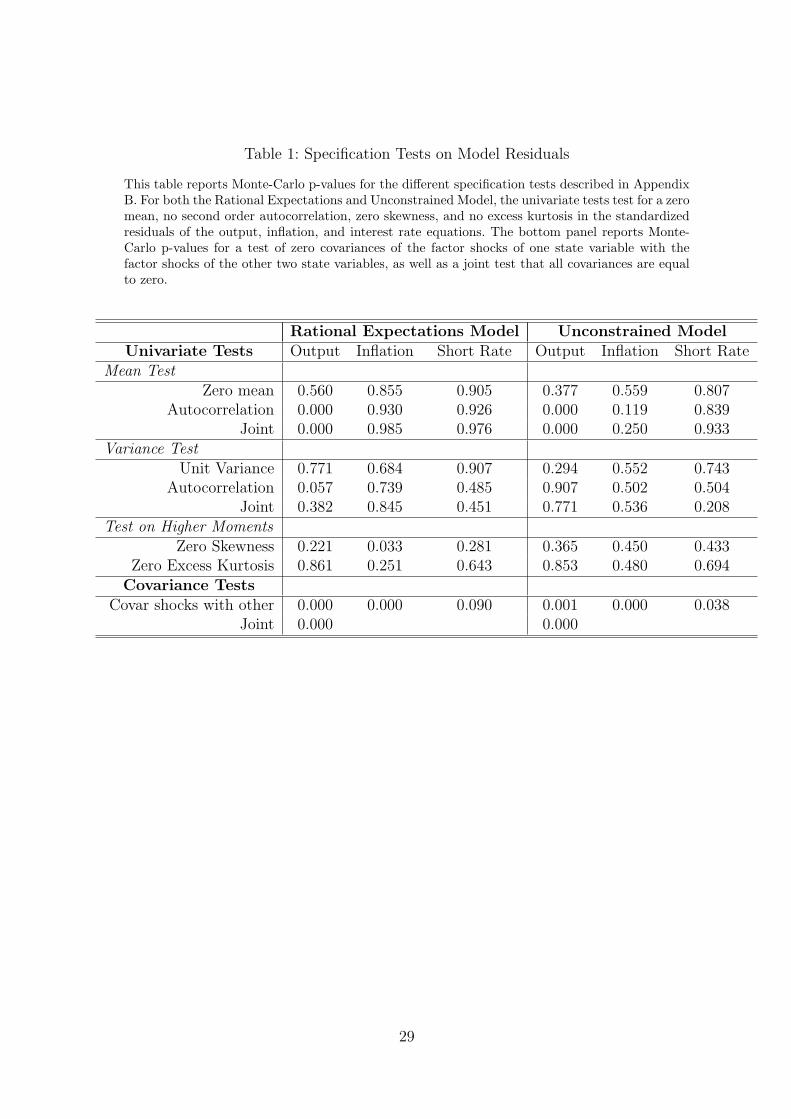
Table 1: Specification Tests on Model Residuals
This table reports Monte-Carlo p-values for the different specification tests described in AppendixB. For both the Rational Expectations and Unconstrained Model, the univariate tests test for a zeromean, no second order autocorrelation, zero skewness, and no excess kurtosis in the standardizedresiduals of the output, inflation, and interest rate equations. The bottom panel reports Monte-Carlo p-values for a test of zero covariances of the factor shocks of one state variable with thefactor shocks of the other two state variables, as well as a joint test that all covariances are equalto zero.
Rational Expectations Model Unconstrained ModelUnivariate Tests Output Inflation Short Rate Output Inflation Short Rate
Mean TestZero mean 0.560 0.855 0.905 0.377 0.559 0.807
Autocorrelation 0.000 0.930 0.926 0.000 0.119 0.839Joint 0.000 0.985 0.976 0.000 0.250 0.933
Variance TestUnit Variance 0.771 0.684 0.907 0.294 0.552 0.743
Autocorrelation 0.057 0.739 0.485 0.907 0.502 0.504Joint 0.382 0.845 0.451 0.771 0.536 0.208
Test on Higher MomentsZero Skewness 0.221 0.033 0.281 0.365 0.450 0.433
Zero Excess Kurtosis 0.861 0.251 0.643 0.853 0.480 0.694Covariance Tests
Covar shocks with other 0.000 0.000 0.090 0.001 0.000 0.038Joint 0.000 0.000
29
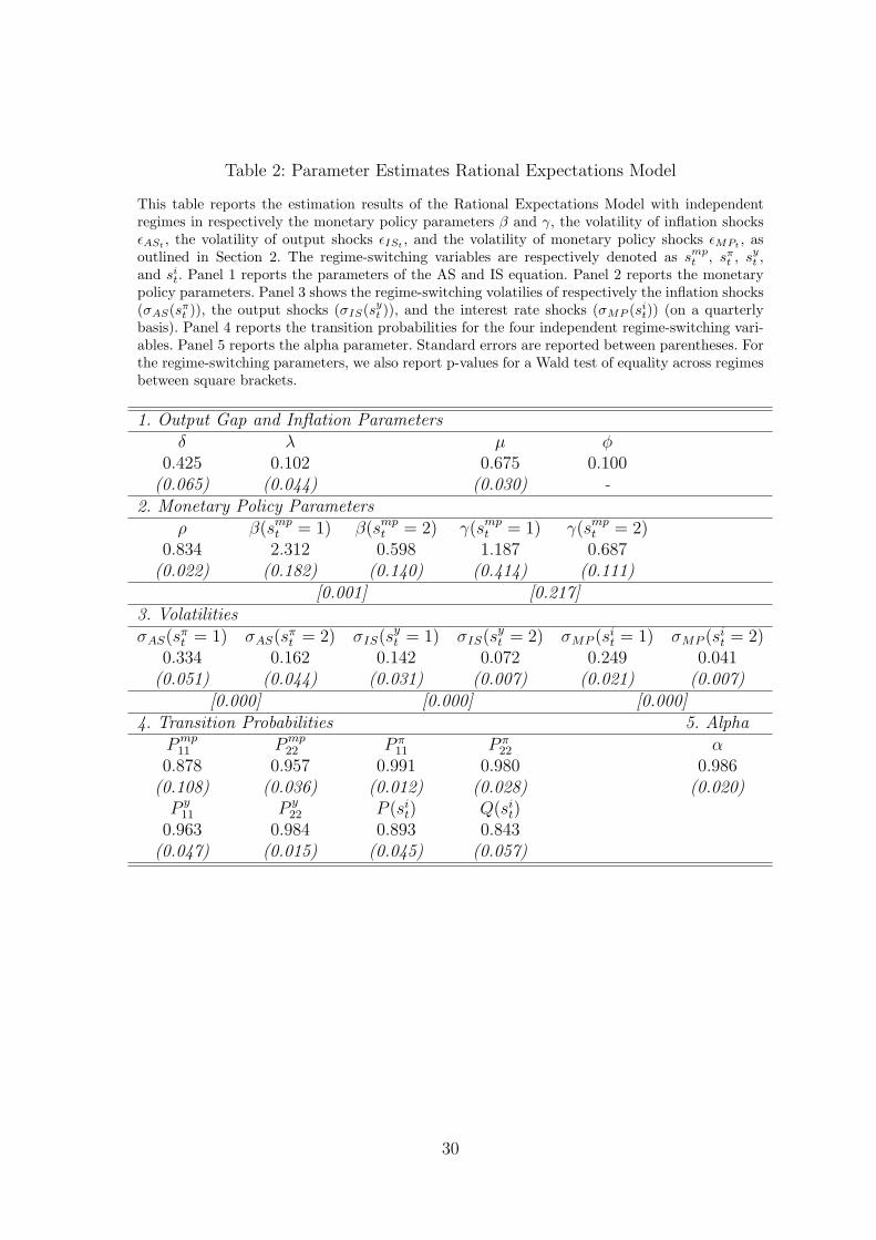
Table 2: Parameter Estimates Rational Expectations Model
This table reports the estimation results of the Rational Expectations Model with independentregimes in respectively the monetary policy parameters β and γ, the volatility of inflation shocksεASt
, the volatility of output shocks εISt, and the volatility of monetary policy shocks εMPt
, asoutlined in Section 2. The regime-switching variables are respectively denoted as smp
t , sπt , sy
t ,and si
t. Panel 1 reports the parameters of the AS and IS equation. Panel 2 reports the monetarypolicy parameters. Panel 3 shows the regime-switching volatilies of respectively the inflation shocks(σAS(sπ
t )), the output shocks (σIS(syt )), and the interest rate shocks (σMP (si
t)) (on a quarterlybasis). Panel 4 reports the transition probabilities for the four independent regime-switching vari-ables. Panel 5 reports the alpha parameter. Standard errors are reported between parentheses. Forthe regime-switching parameters, we also report p-values for a Wald test of equality across regimesbetween square brackets.
1. Output Gap and Inflation Parametersδ λ µ φ
0.425 0.102 0.675 0.100(0.065) (0.044) (0.030) -
2. Monetary Policy Parametersρ β(smp
t = 1) β(smpt = 2) γ(smp
t = 1) γ(smpt = 2)
0.834 2.312 0.598 1.187 0.687(0.022) (0.182) (0.140) (0.414) (0.111)
[0.001] [0.217]3. VolatilitiesσAS(sπ
t = 1) σAS(sπt = 2) σIS(sy
t = 1) σIS(syt = 2) σMP (si
t = 1) σMP (sit = 2)
0.334 0.162 0.142 0.072 0.249 0.041(0.051) (0.044) (0.031) (0.007) (0.021) (0.007)
[0.000] [0.000] [0.000]4. Transition Probabilities 5. Alpha
Pmp11 Pmp
22 P π11 P π
22 α0.878 0.957 0.991 0.980 0.986
(0.108) (0.036) (0.012) (0.028) (0.020)P y
11 P y22 P (si
t) Q(sit)
0.963 0.984 0.893 0.843(0.047) (0.015) (0.045) (0.057)
30
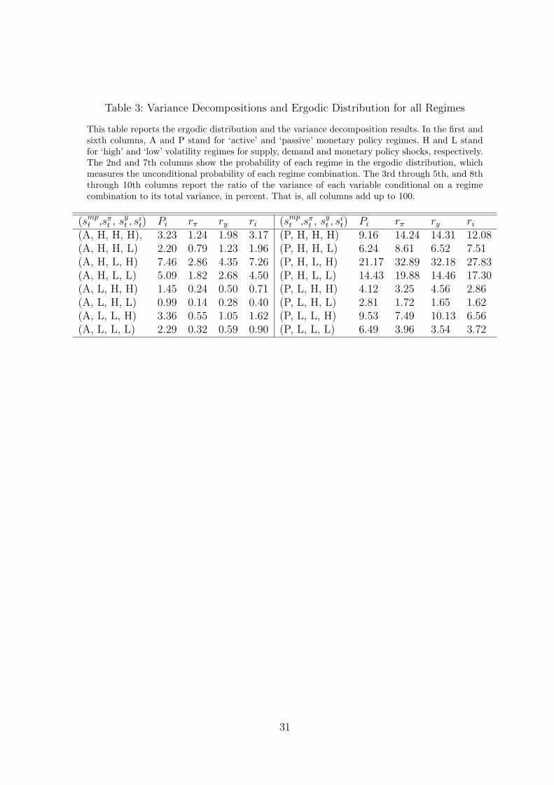
Table 3: Variance Decompositions and Ergodic Distribution for all Regimes
This table reports the ergodic distribution and the variance decomposition results. In the first andsixth columns, A and P stand for ‘active’ and ‘passive’ monetary policy regimes. H and L standfor ‘high’ and ‘low’ volatility regimes for supply, demand and monetary policy shocks, respectively.The 2nd and 7th columns show the probability of each regime in the ergodic distribution, whichmeasures the unconditional probability of each regime combination. The 3rd through 5th, and 8ththrough 10th columns report the ratio of the variance of each variable conditional on a regimecombination to its total variance, in percent. That is, all columns add up to 100.
(smpt ,sπ
t , syt , s
it) Pi rπ ry ri (smp
t ,sπt , sy
t , sit) Pi rπ ry ri
(A, H, H, H), 3.23 1.24 1.98 3.17 (P, H, H, H) 9.16 14.24 14.31 12.08(A, H, H, L) 2.20 0.79 1.23 1.96 (P, H, H, L) 6.24 8.61 6.52 7.51(A, H, L, H) 7.46 2.86 4.35 7.26 (P, H, L, H) 21.17 32.89 32.18 27.83(A, H, L, L) 5.09 1.82 2.68 4.50 (P, H, L, L) 14.43 19.88 14.46 17.30(A, L, H, H) 1.45 0.24 0.50 0.71 (P, L, H, H) 4.12 3.25 4.56 2.86(A, L, H, L) 0.99 0.14 0.28 0.40 (P, L, H, L) 2.81 1.72 1.65 1.62(A, L, L, H) 3.36 0.55 1.05 1.62 (P, L, L, H) 9.53 7.49 10.13 6.56(A, L, L, L) 2.29 0.32 0.59 0.90 (P, L, L, L) 6.49 3.96 3.54 3.72
31
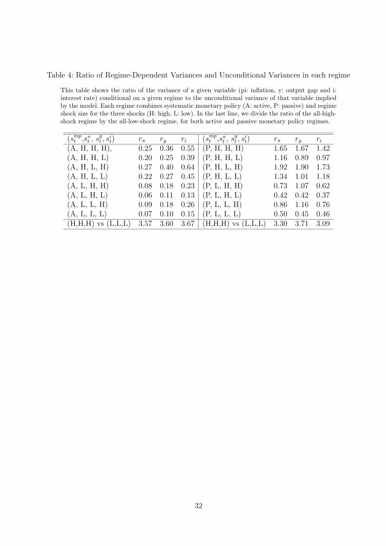
Table 4: Ratio of Regime-Dependent Variances and Unconditional Variances in each regime
This table shows the ratio of the variance of a given variable (pi: inflation, y: output gap and i:interest rate) conditional on a given regime to the unconditional variance of that variable impliedby the model. Each regime combines systematic monetary policy (A: active, P: passive) and regimeshock size for the three shocks (H: high, L: low). In the last line, we divide the ratio of the all-high-shock regime by the all-low-shock regime, for both active and passive monetary policy regimes.
(smpt ,sπ
t , syt , s
it) rπ ry ri (smp
t ,sπt , sy
t , sit) rπ ry ri
(A, H, H, H), 0.25 0.36 0.55 (P, H, H, H) 1.65 1.67 1.42(A, H, H, L) 0.20 0.25 0.39 (P, H, H, L) 1.16 0.89 0.97(A, H, L, H) 0.27 0.40 0.64 (P, H, L, H) 1.92 1.90 1.73(A, H, L, L) 0.22 0.27 0.45 (P, H, L, L) 1.34 1.01 1.18(A, L, H, H) 0.08 0.18 0.23 (P, L, H, H) 0.73 1.07 0.62(A, L, H, L) 0.06 0.11 0.13 (P, L, H, L) 0.42 0.42 0.37(A, L, L, H) 0.09 0.18 0.26 (P, L, L, H) 0.86 1.16 0.76(A, L, L, L) 0.07 0.10 0.15 (P, L, L, L) 0.50 0.45 0.46(H,H,H) vs (L,L,L) 3.57 3.60 3.67 (H,H,H) vs (L,L,L) 3.30 3.71 3.09
32
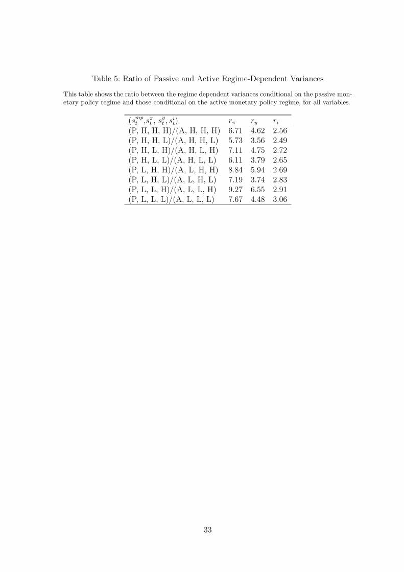
Table 5: Ratio of Passive and Active Regime-Dependent Variances
This table shows the ratio between the regime dependent variances conditional on the passive mon-etary policy regime and those conditional on the active monetary policy regime, for all variables.
(smpt ,sπ
t , syt , s
it) rπ ry ri
(P, H, H, H)/(A, H, H, H) 6.71 4.62 2.56(P, H, H, L)/(A, H, H, L) 5.73 3.56 2.49(P, H, L, H)/(A, H, L, H) 7.11 4.75 2.72(P, H, L, L)/(A, H, L, L) 6.11 3.79 2.65(P, L, H, H)/(A, L, H, H) 8.84 5.94 2.69(P, L, H, L)/(A, L, H, L) 7.19 3.74 2.83(P, L, L, H)/(A, L, L, H) 9.27 6.55 2.91(P, L, L, L)/(A, L, L, L) 7.67 4.48 3.06
33

Tab
le6:
Rob
ust
nes
sTes
ts
Thi
sta
ble
repo
rts
the
stru
ctur
alpa
ram
eter
sλ
and
β,
the
iden
tific
atio
nof
the
Gre
atM
oder
atio
n(G
M)
inte
rms
ofou
tput
and
infla
tion
,an
dth
efr
eque
ncy
ofac
tivi
stsp
ells
for
diffe
rent
spec
ifica
tion
sof
our
Rat
iona
lE
xpec
tati
ons
Mod
el.T
hefir
stco
lum
nre
peat
sth
ere
sult
sof
our
base
line
mod
elw
ith
are
gim
e-sw
itch
ing
γan
dφ
=0.
10.C
olum
ns2
and
3sh
owth
ere
sult
sfo
rth
em
odel
fixin
gφ
atre
spec
tive
ly0.
01an
d0.
20.C
olum
ns4
to6
show
the
resu
lts
for
mod
els
wit
ha
regi
me
inva
rian
tγ.St
anda
rder
rors
are
repo
rted
betw
een
pare
nthe
ses.
Reg
ime-
Sw
itch
ing
γC
onst
ant
γφ
=0.
10φ
=0.
01φ
=0.
20φ
=0.
10φ
=0.
01φ
=0.
20λ
0.10
20.
081
0.11
30.
135
0.07
70.
093
(0.0
44)
(0.0
37)
(0.0
37)
(0.0
35)
(0.0
47)
(0.0
41)
β(s
mp
t=
1)2.
312
2.41
62.
267
2.31
22.
341
2.25
0(0
.182
)(0
.198
)(0
.175
)(0
.182
)(0
.226
)(0
.198
)β
(sm
pt
=2)
0.59
80.
444
0.52
80.
541
0.47
30.
466
(0.1
40)
(0.1
42)
(0.1
34)
(0.1
29)
(0.1
31)
(0.1
42)
Sta
rtdec
line
shock
vari
ability
-O
utp
ut
1981
:419
82:4
1984
:419
81:4
1981
:319
85:2
Sta
rtdec
line
shock
vari
ability
-In
flat
ion
1986
:219
85:4
1990
:219
90:2
1990
:219
86:1
End
low
shock
vari
ability
regi
me
-O
utp
ut
2008
:220
08:2
2008
:120
08:2
2008
:220
07:4
End
low
shock
vari
ability
regi
me
-In
flat
ion
2006
:320
06:3
2005
:420
05:2
2005
:420
06:2
Fre
q.A
ctiv
ist
Spel
lsbef
ore
1980
0.00
00.
000
0.00
00.
000
0.00
00.
000
Fre
q.A
ctiv
ist
Spel
lsaf
ter
1980
0.25
40.
439
0.41
20.
290
0.39
50.
254
34
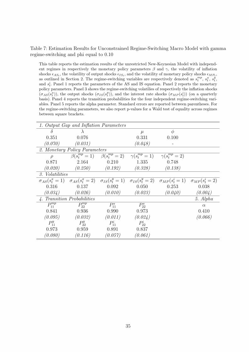
Table 7: Estimation Results for Unconstrained Regime-Switching Macro Model with gammaregime-switching and phi equal to 0.10
This table reports the estimation results of the unrestricted New-Keynesian Model with independ-ent regimes in respectively the monetary policy parameters β and γ, the volatility of inflationshocks εASt
, the volatility of output shocks εISt, and the volatility of monetary policy shocks εMPt
,as outlined in Section 2. The regime-switching variables are respectively denoted as smp
t , sπt , sy
t ,and si
t. Panel 1 reports the parameters of the AS and IS equation. Panel 2 reports the monetarypolicy parameters. Panel 3 shows the regime-switching volatilies of respectively the inflation shocks(σAS(sπ
t )), the output shocks (σIS(syt )), and the interest rate shocks (σMP (si
t)) (on a quarterlybasis). Panel 4 reports the transition probabilities for the four independent regime-switching vari-ables. Panel 5 reports the alpha parameter. Standard errors are reported between parentheses. Forthe regime-switching parameters, we also report p-values for a Wald test of equality across regimesbetween square brackets.
1. Output Gap and Inflation Parametersδ λ µ φ
0.351 0.076 0.331 0.100(0.070) (0.031) (0.048) -
2. Monetary Policy Parametersρ β(smp
t = 1) β(smpt = 2) γ(smp
t = 1) γ(smpt = 2)
0.871 2.164 0.210 1.335 0.748(0.020) (0.250) (0.192) (0.328) (0.138)
3. VolatilitiesσAS(sπ
t = 1) σAS(sπt = 2) σIS(sy
t = 1) σIS(syt = 2) σMP (si
t = 1) σMP (sit = 2)
0.316 0.137 0.092 0.050 0.253 0.038(0.034) (0.026) (0.010) (0.023) (0.040) (0.004)
4. Transition Probabilities 5. AlphaPmp
11 Pmp22 P π
11 P π22 α
0.841 0.936 0.990 0.973 0.410(0.095) (0.032) (0.011) (0.024) (0.066)
P y11 P y
22 P i11 P i
22
0.973 0.959 0.891 0.837(0.080) (0.116) (0.057) (0.061)
35
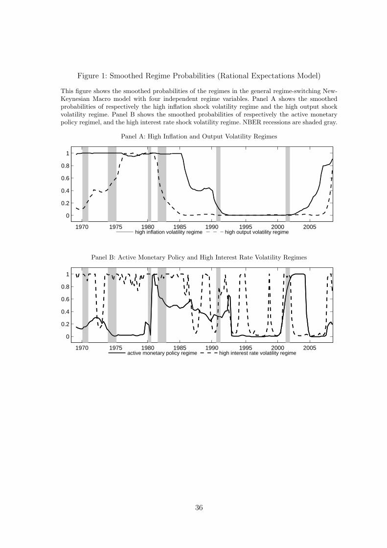
Figure 1: Smoothed Regime Probabilities (Rational Expectations Model)
This figure shows the smoothed probabilities of the regimes in the general regime-switching New-Keynesian Macro model with four independent regime variables. Panel A shows the smoothedprobabilities of respectively the high inflation shock volatility regime and the high output shockvolatility regime. Panel B shows the smoothed probabilities of respectively the active monetarypolicy regimel, and the high interest rate shock volatility regime. NBER recessions are shaded gray.
Panel A: High Inflation and Output Volatility Regimes
1970 1975 1980 1985 1990 1995 2000 2005
0
0.2
0.4
0.6
0.8
1
high inflation volatility regime high output volatility regime
Panel B: Active Monetary Policy and High Interest Rate Volatility Regimes
1970 1975 1980 1985 1990 1995 2000 2005
0
0.2
0.4
0.6
0.8
1
active monetary policy regime high interest rate volatility regime
36
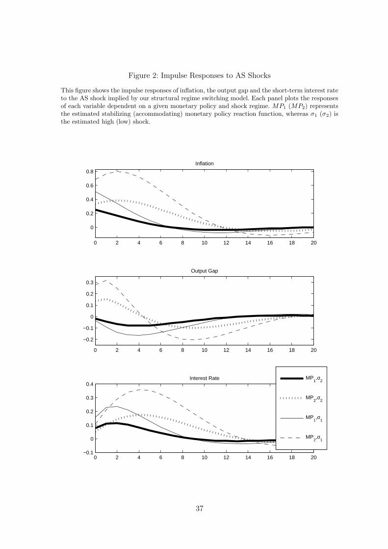
Figure 2: Impulse Responses to AS Shocks
This figure shows the impulse responses of inflation, the output gap and the short-term interest rateto the AS shock implied by our structural regime switching model. Each panel plots the responsesof each variable dependent on a given monetary policy and shock regime. MP1 (MP2) representsthe estimated stabilizing (accommodating) monetary policy reaction function, whereas σ1 (σ2) isthe estimated high (low) shock.
0 2 4 6 8 10 12 14 16 18 20
0
0.2
0.4
0.6
0.8
Inflation
0 2 4 6 8 10 12 14 16 18 20
−0.2
−0.1
0
0.1
0.2
0.3
Output Gap
0 2 4 6 8 10 12 14 16 18 20−0.1
0
0.1
0.2
0.3
0.4Interest Rate MP
1,σ
2
MP2,σ
2
MP1,σ
1
MP2,σ
1
37
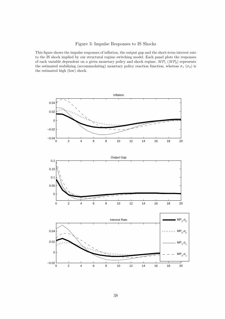
Figure 3: Impulse Responses to IS Shocks
This figure shows the impulse responses of inflation, the output gap and the short-term interest rateto the IS shock implied by our structural regime switching model. Each panel plots the responsesof each variable dependent on a given monetary policy and shock regime. MP1 (MP2) representsthe estimated stabilizing (accommodating) monetary policy reaction function, whereas σ1 (σ2) isthe estimated high (low) shock.
0 2 4 6 8 10 12 14 16 18 20−0.04
−0.02
0
0.02
0.04
Inflation
0 2 4 6 8 10 12 14 16 18 20
0
0.05
0.1
0.15
0.2Output Gap
0 2 4 6 8 10 12 14 16 18 20−0.02
0
0.02
0.04
Interest Rate MP1,σ
2
MP2,σ
2
MP1,σ
1
MP2,σ
1
38

Figure 4: Impulse Responses to MP Shocks
This figure shows the impulse responses of inflation, the output gap and the short-term interestrate to the MP shock implied by our structural regime switching model. Each panel plots theresponses of each variable dependent on a given monetary policy and shock regime. MP1 (MP2)represents the estimated stabilizing (accommodating) monetary policy reaction function, whereasσ1 (σ2) is the estimated high (low) shock.
0 2 4 6 8 10 12 14 16 18 20
−0.5
−0.4
−0.3
−0.2
−0.1
0
Inflation
0 2 4 6 8 10 12 14 16 18 20
−0.4
−0.2
0
0.2Output Gap
0 2 4 6 8 10 12 14 16 18 20
−0.2
−0.1
0
0.1
0.2Interest Rate MP
1,σ
2
MP2,σ
2
MP1,σ
1
MP2,σ
1
39
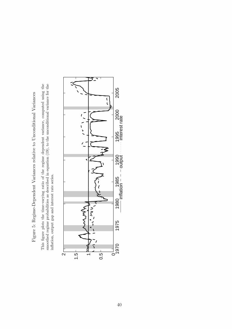
Fig
ure
5:R
egim
e-D
epen
den
tV
aria
nce
sre
lati
veto
Unco
ndit
ional
Var
iance
s
Thi
sfig
ure
plot
sth
eti
me-
vary
ing
rati
oof
the
regi
me
depe
nden
tva
rian
ce,
com
pute
dus
ing
the
smoo
thed
regi
me
prob
abili
ties
asde
scri
bed
ineq
uati
on(1
9),t
oth
eun
cond
itio
nalv
aria
nce
for
the
infla
tion
,ou
tput
gap
and
inte
rest
rate
seri
es.
1970
1975
1980
1985
1990
1995
2000
2005
0
0.51
1.52
infla
tion
outp
utin
tere
st r
ate
40

Fig
ure
6:C
ontr
ibuti
onof
Mon
etar
yPol
icy
toth
eV
olat
ility
[(V
ol(p
assi
ve)/
vol(
X)]
Thi
sfig
ure
plot
sth
evo
lati
lity
rati
obe
twee
nth
eco
unte
rfac
tual
vola
tilit
yof
the
thre
em
acro
vari
-ab
les,
cond
itio
nalo
nth
em
onet
ary
polic
yre
gim
eal
way
sbe
ing
inth
epa
ssiv
ere
gim
e,an
dth
eth
eir
unco
ndit
iona
lvo
lati
lity.
1970
1975
1980
1985
1990
1995
2000
2005
1
1.52
2.53
infla
tion
outp
utin
tere
st r
ate
41
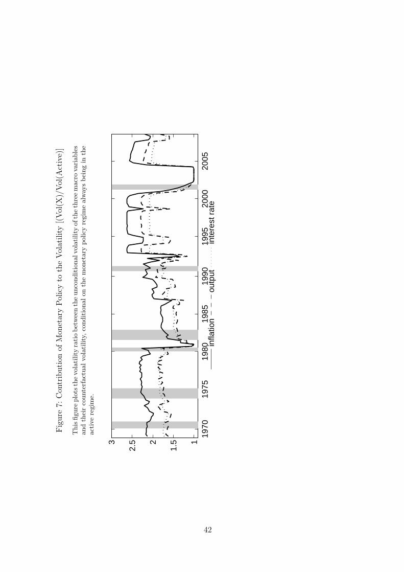
Fig
ure
7:C
ontr
ibuti
onof
Mon
etar
yPol
icy
toth
eV
olat
ility
[(V
ol(X
)/V
ol(A
ctiv
e)]
Thi
sfig
ure
plot
sth
evo
lati
lity
rati
obe
twee
nth
eun
cond
itio
nalv
olat
ility
ofth
eth
ree
mac
rova
riab
les
and
thei
rco
unte
rfac
tual
vola
tilit
y,co
ndit
iona
lon
the
mon
etar
ypo
licy
regi
me
alw
ays
bein
gin
the
acti
vere
gim
e.
1970
1975
1980
1985
1990
1995
2000
2005
1
1.52
2.53
infla
tion
outp
utin
tere
st r
ate
42
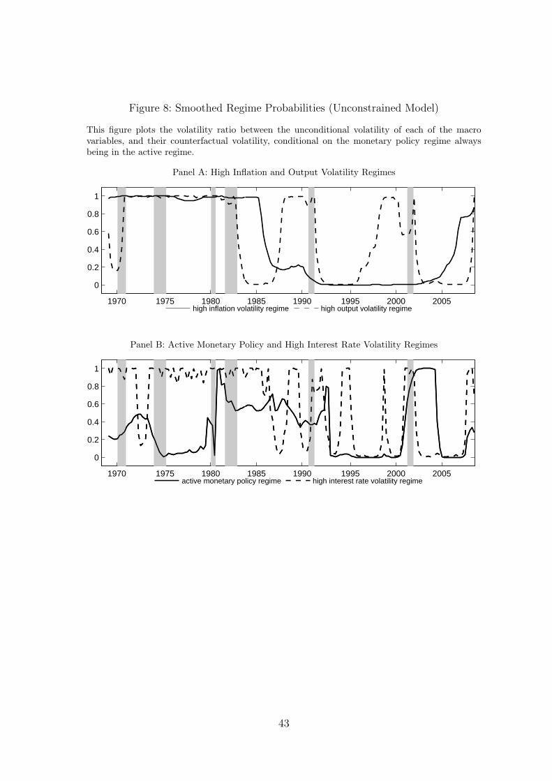
Figure 8: Smoothed Regime Probabilities (Unconstrained Model)
This figure plots the volatility ratio between the unconditional volatility of each of the macrovariables, and their counterfactual volatility, conditional on the monetary policy regime alwaysbeing in the active regime.
Panel A: High Inflation and Output Volatility Regimes
1970 1975 1980 1985 1990 1995 2000 2005
0
0.2
0.4
0.6
0.8
1
high inflation volatility regime high output volatility regime
Panel B: Active Monetary Policy and High Interest Rate Volatility Regimes
1970 1975 1980 1985 1990 1995 2000 2005
0
0.2
0.4
0.6
0.8
1
active monetary policy regime high interest rate volatility regime
43
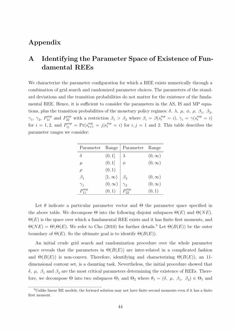
Appendix
A Identifying the Parameter Space of Existence of Fun-
damental REEs
We characterize the parameter configuration for which a REE exists numerically through a
combination of grid search and randomized parameter choices. The parameters of the stand-
ard deviations and the transition probabilities do not matter for the existence of the funda-
mental REE. Hence, it is sufficient to consider the parameters in the AS, IS and MP equa-
tions, plus the transition probabilities of the monetary policy regimes: δ, λ, µ, φ, ρ, β1, β2,
γ1, γ2, Pmp11 and Pmp
22 with a restriction β1 > β2 where βi = β(smpt = i), γi = γ(smp
t = i)
for i = 1, 2, and Pmpij = Pr(smp
t+1 = j|smpt = i) for i, j = 1 and 2. This table describes the
parameter ranges we consider:
Parameter Range Parameter Range
δ (0, 1] λ (0,∞)
µ (0, 1] φ (0,∞)
ρ (0, 1)
β1 [1,∞) β2 (0,∞)
γ1 (0,∞) γ2 (0,∞)
Pmp11 (0, 1) Pmp
22 (0, 1)
Let θ indicate a particular parameter vector and Θ the parameter space specified in
the above table. We decompose Θ into the following disjoint subspaces Θ(E) and Θ(NE).
Θ(E) is the space over which a fundamental REE exists and it has finite first moments, and
Θ(NE) = Θ\Θ(E). We refer to Cho (2010) for further details.5 Let Θ(B(E)) be the outer
boundary of Θ(E). So the ultimate goal is to identify Θ(B(E)).
An initial crude grid search and randomization procedure over the whole parameter
space reveals that the parameters in Θ(B(E)) are inter-related in a complicated fashion
and Θ(B(E)) is non-convex. Therefore, identifying and characterizing Θ(B(E)), an 11-
dimensional contour set, is a daunting task. Nevertheless, the initial procedure showed that
δ, µ, β1 and β2 are the most critical parameters determining the existence of REEs. There-
fore, we decompose Θ into two subspaces Θ1 and Θ2 where θ1 = (δ, µ, β1, β2) ∈ Θ1 and
5Unlike linear RE models, the forward solution may not have finite second moments even if it has a finitefirst moment.
44
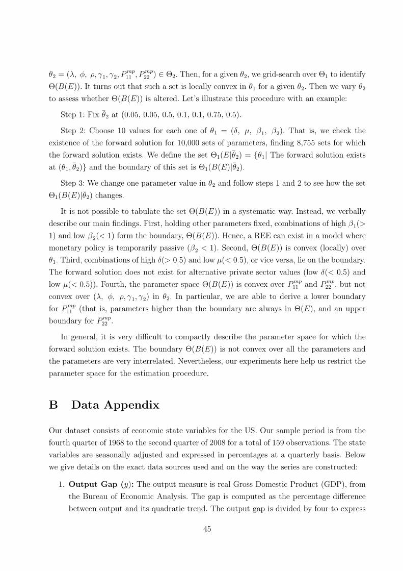
θ2 = (λ, φ, ρ, γ1, γ2, Pmp11 , Pmp
22 ) ∈ Θ2. Then, for a given θ2, we grid-search over Θ1 to identify
Θ(B(E)). It turns out that such a set is locally convex in θ1 for a given θ2. Then we vary θ2
to assess whether Θ(B(E)) is altered. Let’s illustrate this procedure with an example:
Step 1: Fix θ2 at (0.05, 0.05, 0.5, 0.1, 0.1, 0.75, 0.5).
Step 2: Choose 10 values for each one of θ1 = (δ, µ, β1, β2). That is, we check the
existence of the forward solution for 10,000 sets of parameters, finding 8,755 sets for which
the forward solution exists. We define the set Θ1(E|θ2) = θ1| The forward solution exists
at (θ1, θ2) and the boundary of this set is Θ1(B(E)|θ2).
Step 3: We change one parameter value in θ2 and follow steps 1 and 2 to see how the set
Θ1(B(E)|θ2) changes.
It is not possible to tabulate the set Θ(B(E)) in a systematic way. Instead, we verbally
describe our main findings. First, holding other parameters fixed, combinations of high β1(>
1) and low β2(< 1) form the boundary, Θ(B(E)). Hence, a REE can exist in a model where
monetary policy is temporarily passive (β2 < 1). Second, Θ(B(E)) is convex (locally) over
θ1. Third, combinations of high δ(> 0.5) and low µ(< 0.5), or vice versa, lie on the boundary.
The forward solution does not exist for alternative private sector values (low δ(< 0.5) and
low µ(< 0.5)). Fourth, the parameter space Θ(B(E)) is convex over Pmp11 and Pmp
22 , but not
convex over (λ, φ, ρ, γ1, γ2) in θ2. In particular, we are able to derive a lower boundary
for Pmp11 (that is, parameters higher than the boundary are always in Θ(E), and an upper
boundary for Pmp22 .
In general, it is very difficult to compactly describe the parameter space for which the
forward solution exists. The boundary Θ(B(E)) is not convex over all the parameters and
the parameters are very interrelated. Nevertheless, our experiments here help us restrict the
parameter space for the estimation procedure.
B Data Appendix
Our dataset consists of economic state variables for the US. Our sample period is from the
fourth quarter of 1968 to the second quarter of 2008 for a total of 159 observations. The state
variables are seasonally adjusted and expressed in percentages at a quarterly basis. Below
we give details on the exact data sources used and on the way the series are constructed:
1. Output Gap (y): The output measure is real Gross Domestic Product (GDP), from
the Bureau of Economic Analysis. The gap is computed as the percentage difference
between output and its quadratic trend. The output gap is divided by four to express
45
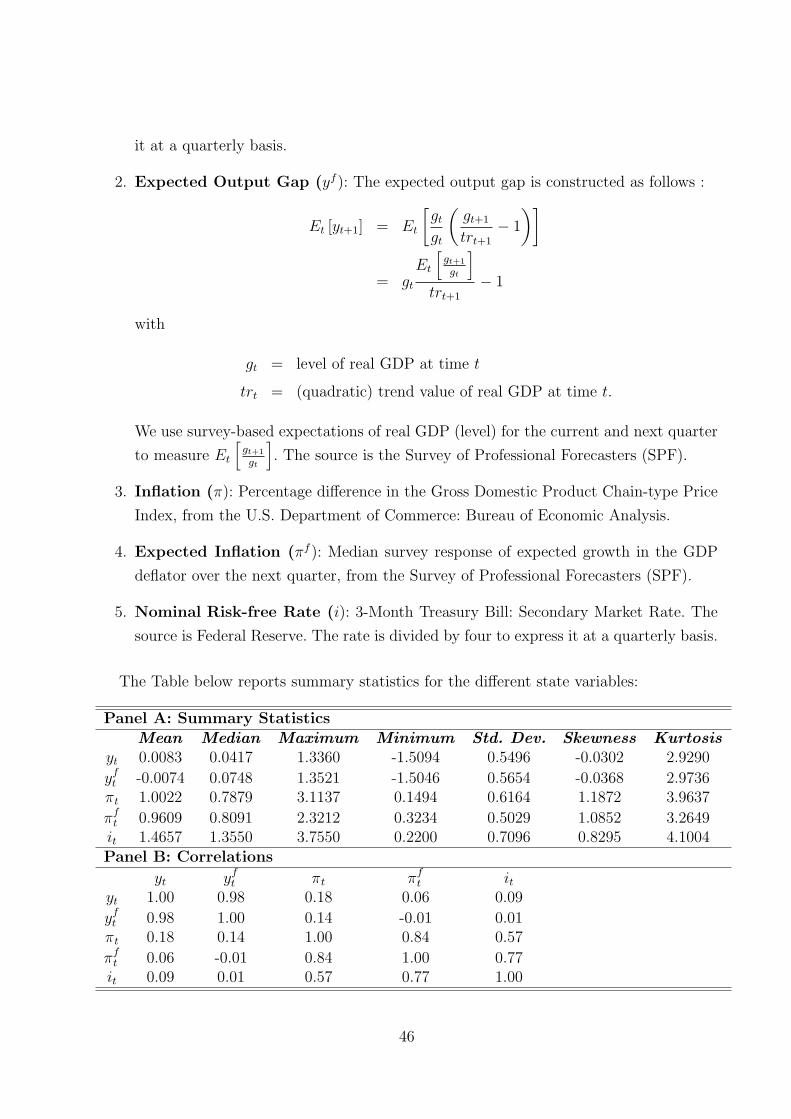
it at a quarterly basis.
2. Expected Output Gap (yf ): The expected output gap is constructed as follows :
Et [yt+1] = Et
[gt
gt
(gt+1
trt+1
− 1
)]
= gt
Et
[gt+1
gt
]
trt+1
− 1
with
gt = level of real GDP at time t
trt = (quadratic) trend value of real GDP at time t.
We use survey-based expectations of real GDP (level) for the current and next quarter
to measure Et
[gt+1
gt
]. The source is the Survey of Professional Forecasters (SPF).
3. Inflation (π): Percentage difference in the Gross Domestic Product Chain-type Price
Index, from the U.S. Department of Commerce: Bureau of Economic Analysis.
4. Expected Inflation (πf ): Median survey response of expected growth in the GDP
deflator over the next quarter, from the Survey of Professional Forecasters (SPF).
5. Nominal Risk-free Rate (i): 3-Month Treasury Bill: Secondary Market Rate. The
source is Federal Reserve. The rate is divided by four to express it at a quarterly basis.
The Table below reports summary statistics for the different state variables:
Panel A: Summary StatisticsMean Median Maximum Minimum Std. Dev. Skewness Kurtosis
yt 0.0083 0.0417 1.3360 -1.5094 0.5496 -0.0302 2.9290
yft -0.0074 0.0748 1.3521 -1.5046 0.5654 -0.0368 2.9736
πt 1.0022 0.7879 3.1137 0.1494 0.6164 1.1872 3.9637
πft 0.9609 0.8091 2.3212 0.3234 0.5029 1.0852 3.2649
it 1.4657 1.3550 3.7550 0.2200 0.7096 0.8295 4.1004Panel B: Correlations
yt yft πt πf
t ityt 1.00 0.98 0.18 0.06 0.09
yft 0.98 1.00 0.14 -0.01 0.01
πt 0.18 0.14 1.00 0.84 0.57
πft 0.06 -0.01 0.84 1.00 0.77
it 0.09 0.01 0.57 0.77 1.00
46

C Specification Tests
The reduced form of the model (see Section 2.4) is given by:
Xt = Ω1(St)Xft−1 + Ω2(St)X
ft + Ω3(St)Xt−1 + Γ(St)εt εt ∼ N(0, Σ(St)), (C-1)
with Σ being the regime-dependent diagonal variance-covariance matrix for the shocks con-
tained in εt. Recall that there are 16 different regimes. Let the smoothed regime probability
for regime i, with a slight abuse of notation, be denoted by Pi,t. That is, Pi,t = P [St = i|It] .
Because regimes are unobserved, the residuals are essentially unobservable to the economet-
rician. We therefore use the econometrician’s best estimate for the residuals given full sample
information and the smoothed probabilities, that is, using equation (15):
εt =S∑
i=1
(Γ(St = i))−1[Xt − Ω1(St)X
ft−1 − Ω2(St)X
ft − Ω3(St)Xt−1
]Pi,t
We denote the regime-dependent variance covariance matrix for these residual, again
with a slight abuse of notation by Vt, that is:
Vt =S∑
i=1
Σ(St = i)Pi,t
We perform our different tests on the standardized residuals zt = V− 1
2t εt. We test for a zero
mean and no second-order correlation by testing whether or not b1, b2, and b3 are zero in:
E [zt]− b1 = 0 (C-2)
E [(zt − b1) (zt−1 − b1)]− b2 = 0 (C-3)
E [(zt − b1) (zt−2 − b1)]− b3 = 0 (C-4)
Define zt = (zt − b1)2 − 1. We test for a well-specified variance by testing whether or not
b4, b5,and b6 are equal to zero in:
E [zt]− b4 = 0
E [ztzt−1]− b5 = 0
E [ztzt−2]− b6 = 0
We test for excess skewness and kurtosis by testing whether or not b7 and b8 are equal to
zero in:
E[(zt − b1)
3]− b7 = 0 (C-5)
47

E[(zt − b1)
4 − 3]− b8 = 0 (C-6)
We estimate b1 to b8 using GMM with a Newey and West (1987) weighting matrix with
number of lags equal to 5. The tests for zero mean, unit variance, zero skewness, and zero
excess kurtosis follow a χ2 (1) distribution, the tests for second order autocorrelation a χ2 (2)
distribution. The joint mean and variance tests follow a χ2 (3) distribution. We also perform
a small sample analysis of the test statistics. For each series, we use the estimated parameters
from the model to simulate a time-series of similar length as our sample. For 500 of such
simulated time-series, we calculate the test statistics, and use the resulting distribution to
derive empirical probability values.
To investigate whether our model adequately captures the covariance between the factor
shocks, we test whether the following conditions hold:
E [zl,tzj,t] = 0, for l, j ∈ yt, πt, it ; l 6= j.
We test for each of the 3 variables whether its shocks have a zero covariance with the two
other shocks. This test follows a χ2 distribution with 2 degrees of freedom. In addition,
we report the joint test for the covariances between all factor shocks which follows a χ2
distribution with 3 degrees of freedom. Our p-values results from a small sample analysis of
the test statistics, analogous to that performed for the univariate tests.
D Impulse Response Analysis
Recall from equation (8) that the forward solution of the REE can be characterized as follows:
Xt = Ω∗(St)Xt−1 + Γ∗(St)εt εt ∼ N(0, Σ(St)).
Conditional on time t information including St, the one-step ahead prediction of Xt+1 is
given by EtXt+1 = F (St, 1)Xt where F (St, 1) = E[Ω∗(St+1)|St]. The k-step ahead prediction
of Xt is then, computed recursively as EtXt+k = F (St, k)Xt where F (St, 0) = I3 and
F (St, k) = E[F (St+1, k − 1)Ω∗(St+1)|St],
for k ≥ 1. The initial value of Xt is given by Γ∗(St)εt. Therefore, the impulse responses of
Xt+k to the initial innovation at time t conditional on St are expressed as:
IR(St, k) = F (St, k)Γ∗(St)εt, (D-7)
48
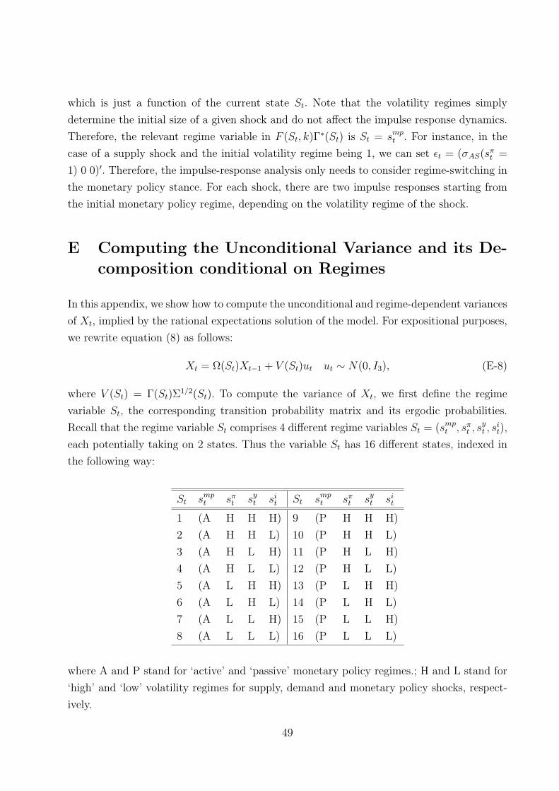
which is just a function of the current state St. Note that the volatility regimes simply
determine the initial size of a given shock and do not affect the impulse response dynamics.
Therefore, the relevant regime variable in F (St, k)Γ∗(St) is St = smpt . For instance, in the
case of a supply shock and the initial volatility regime being 1, we can set εt = (σAS(sπt =
1) 0 0)′. Therefore, the impulse-response analysis only needs to consider regime-switching in
the monetary policy stance. For each shock, there are two impulse responses starting from
the initial monetary policy regime, depending on the volatility regime of the shock.
E Computing the Unconditional Variance and its De-
composition conditional on Regimes
In this appendix, we show how to compute the unconditional and regime-dependent variances
of Xt, implied by the rational expectations solution of the model. For expositional purposes,
we rewrite equation (8) as follows:
Xt = Ω(St)Xt−1 + V (St)ut ut ∼ N(0, I3), (E-8)
where V (St) = Γ(St)Σ1/2(St). To compute the variance of Xt, we first define the regime
variable St, the corresponding transition probability matrix and its ergodic probabilities.
Recall that the regime variable St comprises 4 different regime variables St = (smpt , sπ
t , syt , s
it),
each potentially taking on 2 states. Thus the variable St has 16 different states, indexed in
the following way:
St smpt sπ
t syt si
t St smpt sπ
t syt si
t
1 (A H H H) 9 (P H H H)
2 (A H H L) 10 (P H H L)
3 (A H L H) 11 (P H L H)
4 (A H L L) 12 (P H L L)
5 (A L H H) 13 (P L H H)
6 (A L H L) 14 (P L H L)
7 (A L L H) 15 (P L L H)
8 (A L L L) 16 (P L L L)
where A and P stand for ‘active’ and ‘passive’ monetary policy regimes.; H and L stand for
‘high’ and ‘low’ volatility regimes for supply, demand and monetary policy shocks, respect-
ively.
49
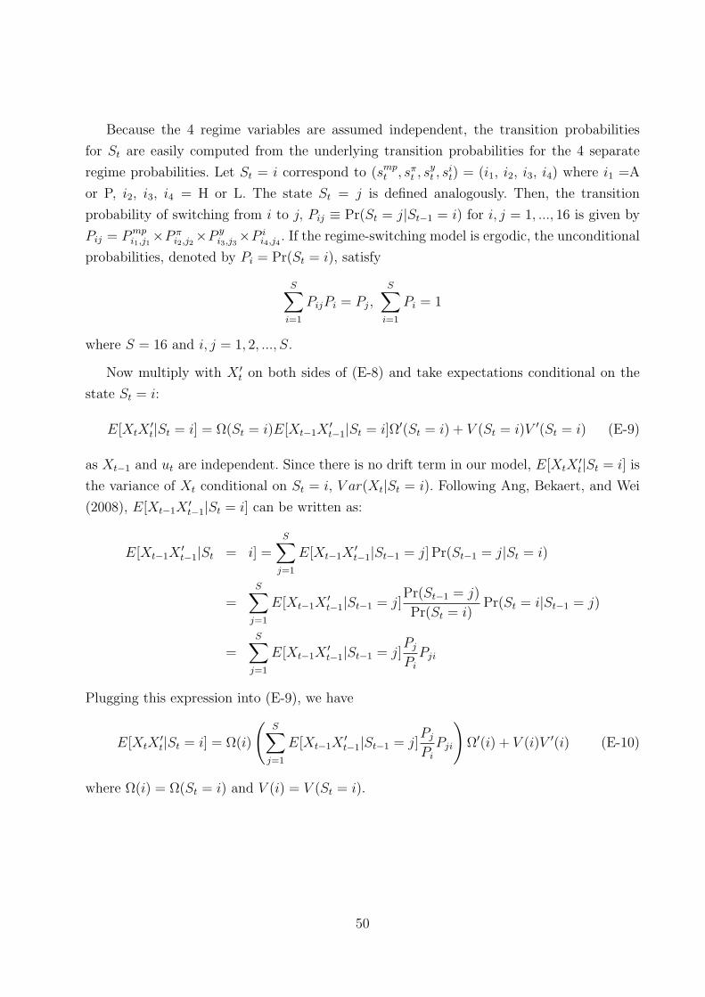
Because the 4 regime variables are assumed independent, the transition probabilities
for St are easily computed from the underlying transition probabilities for the 4 separate
regime probabilities. Let St = i correspond to (smpt , sπ
t , syt , s
it) = (i1, i2, i3, i4) where i1 =A
or P, i2, i3, i4 = H or L. The state St = j is defined analogously. Then, the transition
probability of switching from i to j, Pij ≡ Pr(St = j|St−1 = i) for i, j = 1, ..., 16 is given by
Pij = Pmpi1,j1
×P πi2,j2
×P yi3,j3
×P ii4,j4
. If the regime-switching model is ergodic, the unconditional
probabilities, denoted by Pi = Pr(St = i), satisfy
S∑i=1
PijPi = Pj,S∑
i=1
Pi = 1
where S = 16 and i, j = 1, 2, ..., S.
Now multiply with X ′t on both sides of (E-8) and take expectations conditional on the
state St = i:
E[XtX′t|St = i] = Ω(St = i)E[Xt−1X
′t−1|St = i]Ω′(St = i) + V (St = i)V ′(St = i) (E-9)
as Xt−1 and ut are independent. Since there is no drift term in our model, E[XtX′t|St = i] is
the variance of Xt conditional on St = i, V ar(Xt|St = i). Following Ang, Bekaert, and Wei
(2008), E[Xt−1X′t−1|St = i] can be written as:
E[Xt−1X′t−1|St = i] =
S∑j=1
E[Xt−1X′t−1|St−1 = j] Pr(St−1 = j|St = i)
=S∑
j=1
E[Xt−1X′t−1|St−1 = j]
Pr(St−1 = j)
Pr(St = i)Pr(St = i|St−1 = j)
=S∑
j=1
E[Xt−1X′t−1|St−1 = j]
Pj
Pi
Pji
Plugging this expression into (E-9), we have
E[XtX′t|St = i] = Ω(i)
(S∑
j=1
E[Xt−1X′t−1|St−1 = j]
Pj
Pi
Pji
)Ω′(i) + V (i)V ′(i) (E-10)
where Ω(i) = Ω(St = i) and V (i) = V (St = i).
50

In order to obtain a closed form expression for E[XtX′t|St = i], we define vx and v as
follows:
vx =
vec(E[XtX′t|St = 1])
vec(E[XtX′t|St = 2])
...
vec(E[XtX′t|St = 16])
, v =
vec(V (1)V ′(1))
vec(V (2)V ′(2))
...
vec(V (16)V ′(16))
Then, equation (E-9) for all i = 1, ..., S can be expressed as:
vx = ΣΩvx + v, (E-11)
where (i, j)-th element of the matrix ΣΩ is given by:
ΣΩij = [
Pj
Pi
PjiΩ(i)⊗ Ω(i)].
Therefore, vx = (In2S − ΣΩ)−1v where n = 3. By reshaping vx back into a matrix form, we
have the formula for E[XtX′t|St = i] for all i = 1, 2, ..., S. Finally, V ar(Xt) = E(XtX
′t) can
be obtained as:
V ar(Xt) = E(XtX′t) = E (E[XtX
′t|St])
=S∑
i=1
E[XtX′t|St = i] · Pi
=S∑
i=1
V ar[Xt|St = i] · Pi.
51


![Moderation process for dummies [Read-Only] - pdfMachine ... · 1. PLAN FOR MODERATION Before you can start with Moderation, ask the following questions first:-Who asked for moderation?-Why](https://img.pdfslide.net/doc/110x75/5bc5d2c209d3f264788dfdf4/moderation-process-for-dummies-read-only-pdfmachine-1-plan-for-moderation.jpg)