Macroeconomic stability and economicgrowth in developing countries

Author:Pål Bergset Ulvedal

Supervisor:Prof. Halvor Mehlum

Master of Philosophy in EconomicsDepartment of Economics

University of Oslo

May, 2013

©Pål Bergset Ulvedal

2013

Macroeconomic stability and economic growth in developing countries

Pål Bergset Ulvedal

http://www.duo.uio.no

Print: Reprosentralen, University of Oslo

PREFACE

Writing this thesis has been an experience that has taught me a lot. It wouldnot have been possible without all the help I have gotten from friends, familyand helpful academic staff at the university. I want to thank my supervisorHalvor Mehlum for guiding me through this work, giving me useful ideas andinputs and motivating me. Thanks to Morten H. Grindaker and Thom Åby-holm for a good collaboration and to Eivind H. Olsen, Bjørn G. Johansen,Eirik Brandås, Frikk Nesje, Sarah Anderson, Mari B. Solheim, Asbjørn Rød-seth and Andreas Kotsadam for useful discussions and comments. Thanks toMichael F. Bleaney for inspiring me to replicate his analysis and for helpingme understand some of the technicalities in it.

I also want to thank my family for supporting me and believing in me,and especially my nephews Olai and Peder for reminding me that there existsa life outside Stata – and for being an inspiration.

Last, but not least, I want to thank Ingunn (who hates this thesis morethan anything) for being so loving and patient.

SUMMARY

Understanding how policy measures affect long term economic growth in de-veloping countries is not only an interesting academic topic, but a topic ofsevere importance for the billions of people living in poverty today. A muchdebated topic in the 1990s was the relationship between macroeconomic poli-cies and growth in developing countries. This debate was made relevant bythe structural adjustment programs initiated by the World Bank and the IMFto make developing countries pursue policies that they perceived to be pro-moting growth. An important part of these structural adjustment programswas promote a stable macroeconomic framework.

One of many research papers investigating the relationship between macro-economic stability and economic growth is Michael Bleaney’s (1996) "Macro-economic stability, investment and growth in developing countries" publishedin Journal of development economics. He intended to test whether the qualityof macroeconomic management has any impact on investment and growth:

Any [exogenous] shock to the economic system is likely to be re-flected in macroeconomic statistics. [. . . ] [G]overnment policycan influence the reaction to the shock but not the shock itself.The issue here is the ability of the government to minimise thedestabilising impact of such shocks and to avoid creating unneces-sary macroeconomic uncertainty by its own policy decisions. Docountries which are successful in doing this [. . . ] experience signif-icantly higher rates of investment and faster output growth ratesthan those which fail?(Bleaney, 1996, p. 465)

To investigate this question, he does a cross section regression analysis of41 developing countries. He finds some evidence that his measures of policyinduced macroeconomic instability are significantly negatively associated withgrowth, when controlling for the level of investments. However, he findsno conclusive evidence for a significant association between macroeconomicinstability and investment.

Seventeen years has passed since Bleaney (1996) published his article,and since then the debate in the growth literature has emphasized otherfactors that determine growth. Recent research within the growth literaturehave emphasized the importance of such factors as institutions, culture andgeography in determining growth rates (Acemoglu, 2009). These are alsovariables that are very persistent over time. If these variables are correlated

with Bleaney’s indicators of macroeconomic mismanagement, his estimateswould be biased. Do his results still hold when the analysis is extended andcountry specific effects are controlled for? The purpose of this thesis is toanswer that question. The amount of available data is far greater now than17 years ago. I exploit the opportunities that this additional data gives bydoing extended cross section regressions and panel data regressions.

Bleaney (1996) uses the central government budget surplus, real exchangerate volatility, government debt level and the inflation rate as indicators ofmacroeconomic (in)stability. His results show a negative correlation betweenbudget deficits and growth, and between real exchange rate volatility andgrowth. I find evidence that high government debt and very high inflationrates are detrimental to economic growth, but I find no evidence that budgetdeficits or real exchange rate volatility are significantly associated to growth.Neither do I find conclusive evidence that any of the indicators have anyimpact on the investment rate. I show that Bleaney’s results are little robustto exclusion of outliers, and that his results can possibly be explained byomitted variable biases.

Though my results show a statistically significant negative association be-tween initial government debt and growth, and between inflation and growth,the economic significance seems to be weak. I investigate whether a thresholdmodel rather than a linear relationship seems to fit the data better and findevidence that it does. I propose that the initial government debt level and in-flation rate have no effect on growth at moderate levels, but when they reachunsustainable levels, they have a serious negative impact on growth rates. Totest this hypothesis I include dummy variables for initial government debtabove 90 % and average inflation rate above 25 % in the regressions. Theresults show that the threshold model fits better to the data than the lin-ear model, and that reaching unsustainable levels of government debt andinflation has a strong negative impact on growth rates.

Bleaney (1996) interprets his results as an indication that policy inducedmacroeconomic instability impedes growth. I find this statement too general,and argue that it is necessary to look at each of the indicators individually.I argue that my results can be explained by debt overhangs preventing gov-ernments from getting access to credits, and thus inhibiting public – andpossibly also private – investment, and by economic contractions during in-flation crises.

CONTENTS

1. Introduction . . . . . . . . . . . . . . . . . . . . . . . . . . . . . . . 1

2. Theory . . . . . . . . . . . . . . . . . . . . . . . . . . . . . . . . . . 42.1 The effect of macroeconomic instability on investments . . . . 52.2 Links between investment and growth . . . . . . . . . . . . . . 6

2.2.1 Investment generated growth . . . . . . . . . . . . . . 62.2.2 Other explanations to the relationship . . . . . . . . . 8

2.3 Relative prices and allocation of factors of production . . . . . 92.4 Outward orientation, instability and industrial clusters . . . . 9

3. Methodology . . . . . . . . . . . . . . . . . . . . . . . . . . . . . . 133.1 The framework used by Bleaney (1996) . . . . . . . . . . . . . 133.2 Extending the analysis . . . . . . . . . . . . . . . . . . . . . . 143.3 Endogeniety of the investment rate . . . . . . . . . . . . . . . 16

4. Measuring the quality of macroeconomic management . . . . . . . . 17

5. Results . . . . . . . . . . . . . . . . . . . . . . . . . . . . . . . . . . 205.1 Replication of Bleaney (1996) . . . . . . . . . . . . . . . . . . 225.2 Adding more countries, and looking at the 1990s and 2000s . . 245.3 Panel regression . . . . . . . . . . . . . . . . . . . . . . . . . . 26

6. Discussion . . . . . . . . . . . . . . . . . . . . . . . . . . . . . . . . 286.1 Outliers . . . . . . . . . . . . . . . . . . . . . . . . . . . . . . 296.2 Endogeneity problems . . . . . . . . . . . . . . . . . . . . . . 326.3 Specification . . . . . . . . . . . . . . . . . . . . . . . . . . . . 346.4 Mechanisms . . . . . . . . . . . . . . . . . . . . . . . . . . . . 36

6.4.1 Debt overhang . . . . . . . . . . . . . . . . . . . . . . . 376.4.2 High inflation . . . . . . . . . . . . . . . . . . . . . . . 38

6.5 Heterogeneous effects . . . . . . . . . . . . . . . . . . . . . . . 39

7. Conclusion . . . . . . . . . . . . . . . . . . . . . . . . . . . . . . . . 40

References . . . . . . . . . . . . . . . . . . . . . . . . . . . . . . . . . . 43

Appendix A. Variable descriptions and data sources . . . . . . . . . . 44

Appendix B. Figures and tables . . . . . . . . . . . . . . . . . . . . . . 46

LIST OF TABLES

1 Correlation between mean and standard deviation of inflationrate . . . . . . . . . . . . . . . . . . . . . . . . . . . . . . . . 18

2 The results of Bleaney (1996) . . . . . . . . . . . . . . . . . . 213 OLS same countries as Bleaney 1980-1990 . . . . . . . . . . . 234 Extended OLS . . . . . . . . . . . . . . . . . . . . . . . . . . . 245 Panel regression . . . . . . . . . . . . . . . . . . . . . . . . . . 26

6 Coefficient estimates after excluding outliers . . . . . . . . . . 307 Dummies for high debt and inflation (in the panel regression) 35

8 Coefficient estimates on control variables (OLS regression) . . 479 Coefficient estimates on control variables (panel regression) . 4710 List of countries included in the regressions . . . . . . . . . . 4811 Main dataset . . . . . . . . . . . . . . . . . . . . . . . . . . . 49

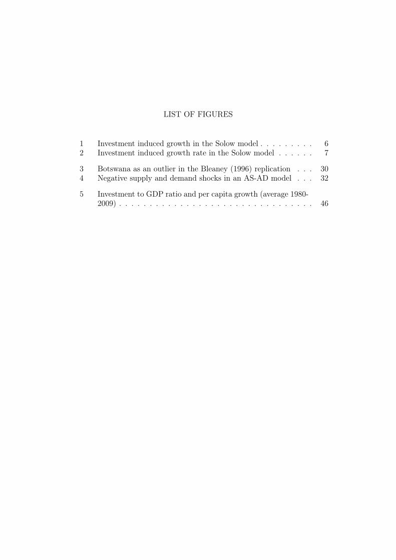
LIST OF FIGURES

1 Investment induced growth in the Solow model . . . . . . . . . 62 Investment induced growth rate in the Solow model . . . . . . 7

3 Botswana as an outlier in the Bleaney (1996) replication . . . 304 Negative supply and demand shocks in an AS-AD model . . . 32

5 Investment to GDP ratio and per capita growth (average 1980-2009) . . . . . . . . . . . . . . . . . . . . . . . . . . . . . . . . 46

1. INTRODUCTION

Understanding how policy measures affect long term economic growth in de-veloping countries is not only an interesting academic topic, but a topic ofsevere importance for the billions of people living in poverty today. A muchdebated topic in the 1990s was the relationship between macroeconomic poli-cies and growth in developing countries. This debate was made relevant bythe structural adjustment programs initiated by the World Bank and theIMF to make developing countries pursue a policy that they perceived to bepromoting growth:

Macroeconomic stability and rapid export growth were two key ele-ments in starting the virtuous circles of high rates of accumulation,efficient allocation and strong productivity growth that formed thebasis for East Asia’s success.(World Bank, 1993, p. 105)

There are several earlier works trying to find empirical evidence for an as-sociation between different indicators of macroeconomic stability or macroe-conomic mismanagement and growth. One well known contribution is a paperby Dani Rodrik (1999). He focuses on how the interaction between underly-ing conflicts between different groups within a country and bad institutionsof conflict management disables countries from implementing the necessarymacroeconomic adjustments to external shocks, and how this harms long termeconomic growth. Other influential contributions are Kormendi and Meguire(1985) who find support for Robert Barro’s (1980) hypothesis that variabilityin the money supply adversely affects growth, Stanley Fischer (1993) whofinds significantly negative correlations between inflation rates, governmentbudget deficit and currency overvaluation and economic growth in a sample of101 developed and developing countries, and Michael Bleaney (1996), who’sanalysis this paper is based on.

Bleaney (1996) intended to test whether the quality of macroeconomicmanagement has any impact on investment and growth:

Any [exogenous] shock to the economic system is likely to be re-flected in macroeconomic statistics. [. . . ] [G]overnment policycan influence the reaction to the shock but not the shock itself.The issue here is the ability of the government to minimise thedestabilising impact of such shocks and to avoid creating unneces-sary macroeconomic uncertainty by its own policy decisions. Do

1. Introduction 2

countries which are successful in doing this [. . . ] experience signif-icantly higher rates of investment and faster output growth ratesthan those which fail?(Bleaney, 1996, p. 465)

To investigate this question, he does a cross section regression analysis of41 developing countries. He finds some evidence that his measures of policyinduced macroeconomic instability are significantly negatively associated withgrowth, when controlling for the level of investments. However, he findsno conclusive evidence for a significant association between macroeconomicinstability and investment.

17 years has passed since Bleaney (1996) published his article, and sincethen the debate in the growth literature has emphasized other factors thatdetermine growth. Recent research within the growth literature have empha-sized the importance of such factors as institutions, culture and geographyin determining growth rates (Acemoglu, 2009). These are also variables thatare very persistent over time. If these variables are correlated with Bleaney’sindicators of macroeconomic mismanagement, his estimates would be biased.Do his results still hold when the analysis is extended and country specific ef-fects are controlled for? The purpose of this thesis is to answer this question.The amount of available data is far greater now than 17 years ago. I willexploit the opportunities that this additional data gives by doing extendedcross section regressions and fixed effect panel regressions.1

Bleaney (1996) uses the central government budget surplus, real exchangerate volatility, government debt level and the inflation rate as indicators ofmacroeconomic (in)stability. His results show a negative correlation betweenbudget deficits and growth, and between real exchange rate volatility andgrowth. I find evidence that high government debt and very high inflationrates are detrimental to economic growth, but I find no evidence that budgetdeficits or real exchange rate volatility are significantly associated to growth.Neither do I find conclusive evidence that any of the indicators have anyimpact on the investment rate. I show that Bleaney’s results are little robustto exclusion of outliers, and that his results can possibly be explained by anomitted variable bias.

Bleaney (1996, p. 476) interprets his results as an indication that policyinduced macroeconomic instability impedes growth. I find this statementtoo general, and argue that it is necessary to look at each of the indicatorsindividually. I argue that my results can be explained by debt overhangspreventing governments from getting access to credits, and thus inhibitingpublic – and possibly also private – investment, and by economic contractionsduring inflation crises.

I will start by presenting some economic theory that explains the channelsthrough which macroeconomic instability might affect economic growth (inchapter 2). The methodology used by Bleaney (1996) and in this paper will

1 I used Stata to calculate all estimates in this thesis.

1. Introduction 3

be laid out in chapter 3, while the issue of measuring macroeconomic stabilitywill be assessed in chapter 4. The main results are presented in chapter 5.Further investigation and discussion of potential methodological problems aswell as causal linkages will be discussed in chapter 6, before I draw someconcluding remarks in chapter 7.

2. THEORY

The possible theoretical linkages between macroeconomic stability and eco-nomic growth are many. I will not try to give a complete review of them here,but I will highlight some of the possible linkages that I find most relevant.

Before looking into the theories, I find it useful to explain what I meanby macroeconomic stability. The World Bank describes the macroeconomicframework as stable "when the inflation rate is low and predictable, real inter-est rates are appropriate, the real exchange rate is competitive and predictable... and the balance of payments situation is perceived as viable" (World Bank,1990). One could also include stability in output (as measured by GDP) andunemployment rates, which for many is the first thing that comes to mindwhen they think about macroeconomic fluctuations. However, for reasonsexplained below, these are not included as indicators of good macroeconomicmanagement in this thesis.

When facing an external shock, the government may face a dilemma whereit has to choose between stability in inflation, real exchange rates and a viablefiscal policy on the one hand and stability in output and unemployment rateson the other. Choosing stability in the latter at expense of the former is oftenperceived to be bad macroeconomic management, because it is detrimentalto output and unemployment rates in the long run (Kydland and Prescott,1977). I will not enter into a discussion about which policy is best in thelong term. This can probably vary from case to case, depending on a widerange of circumstances. However, I will focus this thesis on the impact thata low and stable inflation, a stable real exchange rate and a viable fiscalpolicy have on growth, ignoring potential effects of fluctuations in outputand unemployment.

I will first look into what economic theory tells us about the effect macroe-conomic instability can be expected to have on investments. If macroeconomicinstability is inhibiting growth through depressing investments, as the WorldBank (1990) believed, it must be so that higher investment rates cause highergrowth rates. Though the empirical evidence of correlation between invest-ment and growth is robust, the causal relationship is far from agreed uponamong economists. I will therefore shortly present theoretical frameworksthat seek to explain this relationship.

In the last two sections of this chapter I will present some theoretical con-siderations on how different aspects of macroeconomic instability can affectgrowth more directly, through its effect on total factor productivity ratherthan through its effect on the investment rate.

2. Theory 5

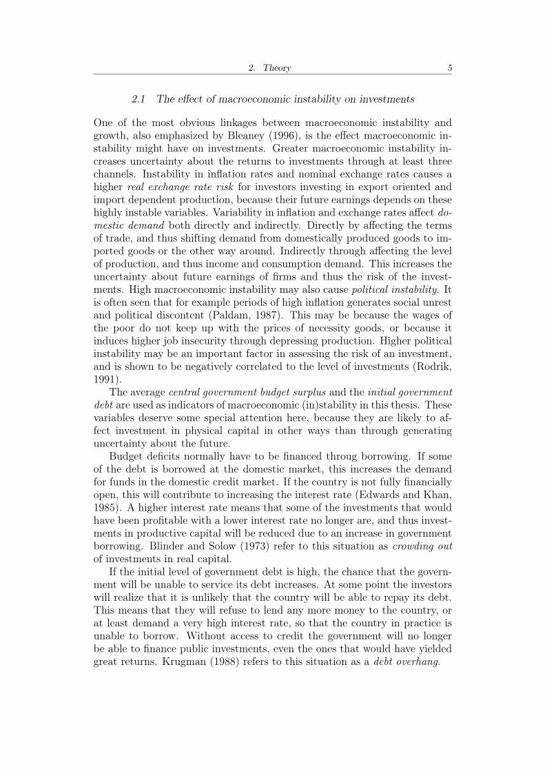
2.1 The effect of macroeconomic instability on investments

One of the most obvious linkages between macroeconomic instability andgrowth, also emphasized by Bleaney (1996), is the effect macroeconomic in-stability might have on investments. Greater macroeconomic instability in-creases uncertainty about the returns to investments through at least threechannels. Instability in inflation rates and nominal exchange rates causes ahigher real exchange rate risk for investors investing in export oriented andimport dependent production, because their future earnings depends on thesehighly instable variables. Variability in inflation and exchange rates affect do-mestic demand both directly and indirectly. Directly by affecting the termsof trade, and thus shifting demand from domestically produced goods to im-ported goods or the other way around. Indirectly through affecting the levelof production, and thus income and consumption demand. This increases theuncertainty about future earnings of firms and thus the risk of the invest-ments. High macroeconomic instability may also cause political instability. Itis often seen that for example periods of high inflation generates social unrestand political discontent (Paldam, 1987). This may be because the wages ofthe poor do not keep up with the prices of necessity goods, or because itinduces higher job insecurity through depressing production. Higher politicalinstability may be an important factor in assessing the risk of an investment,and is shown to be negatively correlated to the level of investments (Rodrik,1991).

The average central government budget surplus and the initial governmentdebt are used as indicators of macroeconomic (in)stability in this thesis. Thesevariables deserve some special attention here, because they are likely to af-fect investment in physical capital in other ways than through generatinguncertainty about the future.

Budget deficits normally have to be financed throug borrowing. If someof the debt is borrowed at the domestic market, this increases the demandfor funds in the domestic credit market. If the country is not fully financiallyopen, this will contribute to increasing the interest rate (Edwards and Khan,1985). A higher interest rate means that some of the investments that wouldhave been profitable with a lower interest rate no longer are, and thus invest-ments in productive capital will be reduced due to an increase in governmentborrowing. Blinder and Solow (1973) refer to this situation as crowding outof investments in real capital.

If the initial level of government debt is high, the chance that the govern-ment will be unable to service its debt increases. At some point the investorswill realize that it is unlikely that the country will be able to repay its debt.This means that they will refuse to lend any more money to the country, orat least demand a very high interest rate, so that the country in practice isunable to borrow. Without access to credit the government will no longerbe able to finance public investments, even the ones that would have yieldedgreat returns. Krugman (1988) refers to this situation as a debt overhang.

2. Theory 6

2.2 Links between investment and growth

If macroeconomic stability promotes growth through the investment chan-nel, it must also be so that investment promotes growth. Empirically, thecorrelation between investment and growth is one of the most statisticallyrobust ones in the growth literature (Levine and Renelt, 1992). However,there exists no consensus on the causal relationship between them. I willtherefore spend some time discussing some theories that can explain thisrelationship. I will first present two models that explain how investmentsgenerate growth, namely the Solow model and the AK model. ThereafterI will present some theoretical explanations to why the correlation betweeninvestment and growth is high even though investment does not generatesustained economic growth.

2.2.1 Investment generated growth

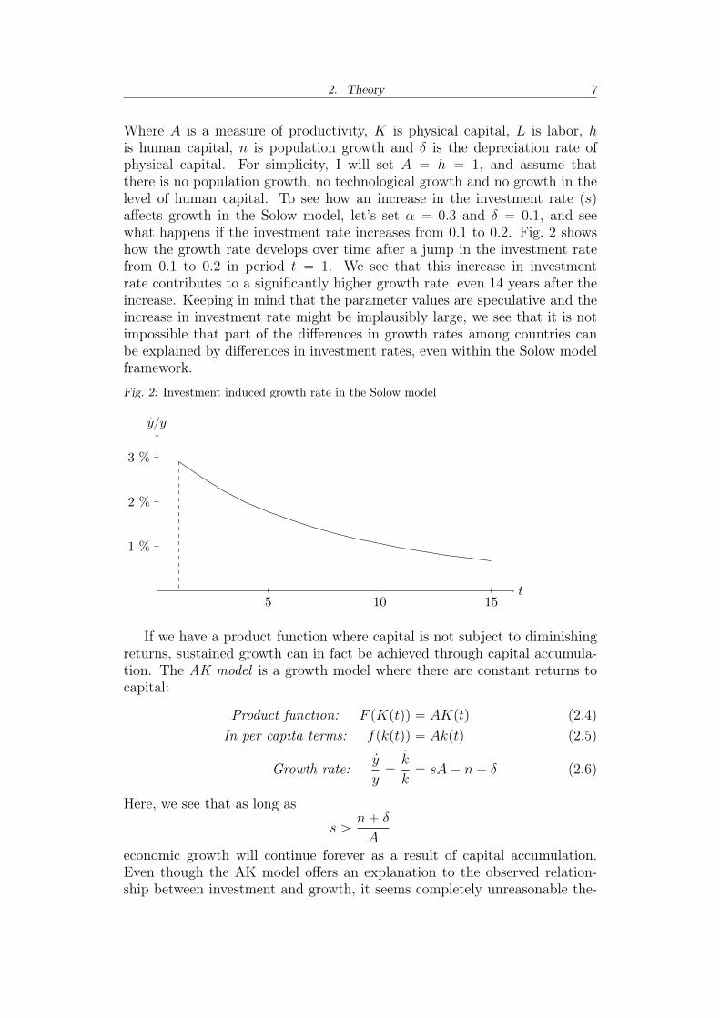
In the classical Solow-Swan model, sustained economic growth can only beachieved through technological progress. Increasing the investment rate willcause an increase in the level of capital per worker, and thus in the per capitaoutput. The growth will continue until the depreciation and dilution of capitalequals investments (see Fig. 1).

Fig. 1: Investment induced growth in the Solow model

k

y “ fpkq

fpkq

s1fpkq

s0fpkq

pn` δqk

k1

y1

k0

y0

This growth is temporary, and only lasts from one steady state to another,but how long this takes depends on the parameter values. To get an ideaabout what the Solow model predicts, let’s take a look at an example:

Product function: F pK,Lq “ AKαphLq1´α, 0 ă α ă 1 (2.1)

In per capita terms: fpkq “ Akαh1´α, k “ K{L (2.2)Steady state: sfpkq “ pn` δqk (2.3)

2. Theory 7

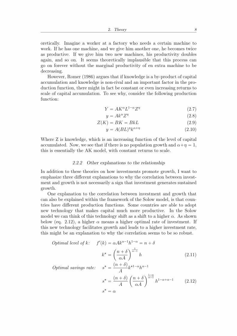
Where A is a measure of productivity, K is physical capital, L is labor, his human capital, n is population growth and δ is the depreciation rate ofphysical capital. For simplicity, I will set A “ h “ 1, and assume thatthere is no population growth, no technological growth and no growth in thelevel of human capital. To see how an increase in the investment rate (s)affects growth in the Solow model, let’s set α “ 0.3 and δ “ 0.1, and seewhat happens if the investment rate increases from 0.1 to 0.2. Fig. 2 showshow the growth rate develops over time after a jump in the investment ratefrom 0.1 to 0.2 in period t “ 1. We see that this increase in investmentrate contributes to a significantly higher growth rate, even 14 years after theincrease. Keeping in mind that the parameter values are speculative and theincrease in investment rate might be implausibly large, we see that it is notimpossible that part of the differences in growth rates among countries canbe explained by differences in investment rates, even within the Solow modelframework.

Fig. 2: Investment induced growth rate in the Solow model

t

9y{y

5 10 15

1 %

2 %

3 %

If we have a product function where capital is not subject to diminishingreturns, sustained growth can in fact be achieved through capital accumula-tion. The AK model is a growth model where there are constant returns tocapital:

Product function: F pKptqq “ AKptq (2.4)In per capita terms: fpkptqq “ Akptq (2.5)

Growth rate:9y

y“

9k

k“ sA´ n´ δ (2.6)

Here, we see that as long as

s ąn` δ

Aeconomic growth will continue forever as a result of capital accumulation.Even though the AK model offers an explanation to the observed relation-ship between investment and growth, it seems completely unreasonable the-

2. Theory 8

oretically. Imagine a worker at a factory who needs a certain machine towork. If he has one machine, and we give him another one, he becomes twiceas productive. If we give him two new machines, his productivity doublesagain, and so on. It seems theoretically implausible that this process cango on forever without the marginal productivity of en extra machine to bedecreasing.

However, Romer (1986) argues that if knowledge is a by-product of capitalaccumulation and knowledge is non-rival and an important factor in the pro-duction function, there might in fact be constant or even increasing returns toscale of capital accumulation. To see why, consider the following productionfunction:

Y “ AKαL1´αZη (2.7)y “ AkαZη (2.8)

ZpKq “ BK “ BkL (2.9)y “ ApBLqηkα`η (2.10)

Where Z is knowledge, which is an increasing function of the level of capitalaccumulated. Now, we see that if there is no population growth and α`η “ 1,this is essentially the AK model, with constant returns to scale.

2.2.2 Other explanations to the relationship

In addition to these theories on how investments promote growth, I want toemphasize three different explanations to why the correlation between invest-ment and growth is not necessarily a sign that investment generates sustainedgrowth.

One explanation to the correlation between investment and growth thatcan also be explained within the framework of the Solow model, is that coun-tries have different production functions. Some countries are able to adoptnew technology that makes capital much more productive. In the Solowmodel we can think of this technology shift as a shift to a higher α. As shownbelow (eq. 2.12), a higher α means a higher optimal rate of investment. Ifthis new technology facilitates growth and leads to a higher investment rate,this might be an explanation to why the correlation seems to be so robust.

Optimal level of k: f 1pkq “ αAkα´1h1´α “ n` δ

k˚ “

ˆ

n` δ

αA

˙1

α´1

h (2.11)

Optimal savings rate: s˚ “pn` δq

Ak˚1´αhα´1

s˚ “pn` δq

A

ˆ

n` δ

αA

˙1´αα´1

h1´α`α´1 (2.12)

s˚ “ α

2. Theory 9

The other two explanations can be thought of within the framework of asimple Keynes model. If the economy has free production capacity, and thesupply responds to demand, increased investment would directly lead to ahigher output. This is simply because the investments themselves generateeconomic activity by utilizing workers and capital that would not otherwisebe in use, and not because new machinery or infrastructure makes productionmore efficient.

A third explanation to the relationship is that it is growth that causesinvestments, and not the other way around. This might be because firmsreceive high profits in years of high growth, and they use this profit to investin new capital. It might also be that investors invest more when they expecthigh growth, because high growth means high demand and high profits.

The main message from this section is that it is not clear that investmentsgenerate sustained growth, even though this is often taken for granted by someeconomists. If investments do not generate growth, it cannot be the case thatmacroeconomic stability promotes growth through its effect on investments.

2.3 Relative prices and allocation of factors of production

In addition to the possibility that macroeconomic instability affects growththrough its effect on investment, in this and the following section, I wantto present theories that explain how it can affect productivity more directly.The first theoretical argument, also emphasized by Fischer (1993), is straightforward and focuses on the effect macroeconomic instability has on an efficientresource allocation.

In order for free markets to secure an effective allocation of resources, oneof the conditions that has to be fulfilled is that all actors have accurate infor-mation about relative prices. If inflation is high and unstable, it is hard for aproducer to know what the prices and wages will be in the future. It is alsovery likely that it will be hard to know what the price of the output good willbe relative to the price of inputs, and thus hard to plan how much to produceand how much to use of each input. This can cause large inefficiencies, inthe sense that production will be lower than what would have been possibleif there was certainty about relative prices (Fischer, 1993).

2.4 Outward orientation, instability and industrial clusters

The relationship between trade orientation and economic growth is probablyone of the most debated topics in the growth literature (see e.g. Dollar, 1992;Sachs et al., 1995; Rodriguez and Rodrik, 2001). There is no clear academicconsensus on whether outward orientation promotes growth, and if it does,through which mechanisms it works. Different theories focus on how outwardorientation gives an economy access to financial capital from abroad, to newtechnology and lets the economy increase total factor productivity by movingfactors to sectors in which it has a comparative advantage (Acemoglu, 2009).

2. Theory 10

New trade theory (see e.g. Krugman, 1991) focuses on how access to largermarkets allow countries to benefit from economies of scale. This is the theoryI will use (in this section) to explain how instability, especially through realexchange rate volatility, can have a negative impact on growth.

Underlying the assumption that real exchange rate volatility increasesuncertainty about profits in the export sector, lies a simple profit function,where a firm receives its revenue in foreign currency and pays expenses indomestic currency:

ΠpP˚, E, P q “ RpP˚, Eq ´ CpP q

Where Π is profit, R is the revenue function, C is the cost function, P˚ isthe price level abroad, P is the domestic price level and E is the nominalexchange rate. R is increasing in P˚ and E, while C is increasing in P , andthus Π is increasing in P˚ and E, and declining in C. Since the real exchangerate is defined as RER “ P˚E

Pit is a good approximation that the profits in

the export sector depend positively on the real exchange rate:

BΠ

BRERą 0

For firms producing for the domestic market, but relying on imported inputs,the relationship would be the opposite, but volatility in the real exchangerate will have the same effect for both types of firms. To keep the discussionsimple I will focus on firms in the export sector, but the arguments also holdfor firms producing for the domestic market with imported inputs.

Real exchange rate volatility increases the risk for investments in the ex-port sector, which means that investors would require a high risk premiumfor being willing to invest in the export sector, which in turn will lead to alow level of investments in the export sector. This is only part of the story,because increased exchange rate volatility also means that the frequency offirm bankruptcy will be high in this sector. This is especially true in countrieswith poorly developed financial markets. To illustrate why, I will present avery simple model based on Aghion et al. (2009).

Imagine that in order to continue production in period t` 1 the firm hasto pay a cost I in period t. Think of this as an investment that the firm has todo before every period. If there are no credit constraints, the firm will chooseto pay the cost and continue production, as long as the expected profit inperiod t` 1 is greater than the cost in period t:

It ă βEpΠpRERqt`1q, β “1

1` r

Where r is the discount rate. However, if there are credit constraints anadditional requirement for production to continue is that the firm has enoughliquidity to finance the investment. Let the amount the firm is able to borrowin period t equal pµ ´ 1qΠt, where µ is a measure of financial development.

2. Theory 11

The total amount of liquidity the firm has available in period t is then µΠt.The additional requirement then becomes:

µΠt ą It

Here we assume that the firm does not save any of its profits from one periodto another. This assumption might seem unrealistic, but it might not beunreasonable for small and new firms that have not been able to acquiremuch equity.

We see that if the level of financial development (µ) is low and the realexchange rate was low in one year, the firm might not be able to pay thenecessary cost to continue production in the next year. An implication of anincreased real exchange rate volatility is that, for a given level of financialdevelopment, the likelihood of being unable to finance the cost of continuingproduction increases.

Furthermore, this high frequency of firm bankruptcies might hinder the de-velopment of industrial clusters, where firms benefit from economies of scale.Marshall (1920) showed how industrial clusters may help firms to compete,due to the presence of economies of scale. He focused on three importantsources to economies of scale: The presence of a pool of specialized work-ers, easy access to suppliers of specialized inputs and services and knowledgespillovers between firms. Higher frequency of firms going out of business islikely to reduce the presence of all these positive externalities, and thus hinderdevelopment of the cluster itself.

In an industry cluster where different firms have very specialized tasks, allfirms depend on many other firms. Producers of final goods depend on sub-contractors that deliver very specialized inputs or services, while producersof inputs and services are so specialized that they are dependent on deliv-ering their outputs to specific producers of a final good. Their equipmentand knowledge is so specialized that they cannot easily shift production tosomething else if their costumer goes out of business. If one producer of afinal good goes bankrupt, it is likely that some of the firms delivering in-puts and services to that firm also will go bankrupt. These firms might havebeen crucial to other producers of a final good, and their disappearance maycause problems for that firm, and so on. This puts an effective end to anydevelopment of industrial clusters.

Building up specialized knowledge about production takes time. Thelonger a firm lives, the more knowledge it manages to build up, at least upto a certain age. If knowledge spillover is an important source of economiesof scale, then firms will benefit more from positive externalities, the more oldfirms there are. Hence, a higher rate of firm bankruptcies hinders this sourceof economies of scale.

There are many factors that have to be in place for a cluster to de-velop. Without the economies of scale stemming from specialized suppliersand knowledge spillovers it is also unlikely that a pool of specialized workersshould emerge.

2. Theory 12

Hence, high real exchange rate volatility makes it unlikely that industryclusters develop, and therefore countries with high real exchange rate volatil-ity are unable to take advantage of this aspect of openness.

In this chapter I have shown that macroeconomic instability can be ex-pected to affect growth through at least three channels. The first is theadverse effect it may have on capital accumulation. The second is more di-rectly by inhibiting total factor productivity by making the price mechanismless efficient, causing an efficient allocation of factors of production (Fischer,1993). The third is through hindering development of industrial clusters. Inthe next chapter I will discuss how we can empirically investigate to whatextent macroeconomic instability affects investment and growth.

3. METHODOLOGY

If suitable measures of macroeconomic stability can be found (I will returnto this question in chapter 4), Bleaney (1996) argues that the effects macroe-conomic instability have on growth can be tested through a well establishedframework for empirical testing of growth models (see e.g. Barro, 1991; Levineand Renelt, 1992). In this chapter I will first present the methodologicalframework used by Bleaney (1996). I will then present how I will extend hisanalysis, before I discuss one of the most serious shortcomings of our method-ological frameworks, namely that we ignore the fact that the investment rateis most likely endogenous.

3.1 The framework used by Bleaney (1996)

The framework Bleaney (1996) uses is the following:

GRi “ α ` ψINVi `Xiβ `Ziγ ` εi, i “ 1, ..., n (3.1)

Where GR is the growth rate of GDP per capita, INV is a measure of thegrowth rate of physical capital, X is a vector of control variables, Z is a vectorof indicators of macroeconomic stability and α is a constant. The subscripti denotes that this is the observation for country i. The underlying theorybehind this framework is the neoclassical growth model, with physical andhuman capital and labor as the factors of production. As a proxy to thegrowth rate in physical capital, he uses the ratio of investment to GDP. Thesignificance of this variable in growth regressions is the most consistent resultin previous research (Levine and Renelt, 1992). The variables he chose toinclude as controls were (with some modifications) the variables that Levineand Renelt (1992) found as robust determinants of growth. Their study testedthe robustness of many variables that have been suggested as conducive togrowth. In addition to the investment rate, the variables they identified asrobust were the initial level of per capita GDP, population growth and thelevel of schooling (as measured by the ratio of secondary school enrollment).In addition to these, Bleaney (1996) includes the growth rate of the exportsto GDP ratio as a control variable. He excludes the ratio of secondary schoolenrollment, because it appears as insignificant in his regression.

Including the variables identified as robust by Levine and Renelt (1992)can also be justified from a theoretical point of view, in the sense that outsideof the steady state (and with no technological growth), these are proxies forthe factors that will determine the growth rate in a Solow model, in the short

3. Methodology 14

term. Bleaney (1996) does not go into why he includes the growth rate ofthe exports to GDP ratio as a control variable, but one obvious reason forincluding it is that changes in foreign demand causes an increase in the priceof exports, which automatically will lead to an increase in GDP.

Bleaney (1996) uses a similar framework to test the impact of macroeco-nomic instability on investments:

INVi “ δ ` Viφ`Ziρ` ηi (3.2)

Where Z is the same vector of indicators of macroeconomic stability as ineq. (3.1), V is a vector of control variables and δ is a constant. Levineand Renelt (1992) also tested the robustness of different variables that wereproposed as being conducive to investment. The only variable they identifiedas robust was the exports to GDP ratio as a measure of openness. In additionto using the initial ratio of exports to GDP, Bleaney (1996) uses the averagegrowth rate of the exports/GDP ratio as well as the index of real exchangerate distortion calculated by Dollar (1992) for the period 1976-85.

3.2 Extending the analysis

Due to lack of data on real exchange rate distortion in the 1990s and 2000s, Ihave not included this variable in any other regressions than the replicationof Bleaney (1996). Other than that, I have used the same control variables asBleaney (1996) in all of the regressions in this paper. As a measure of humancapital, I attempted to include the average attended years of education in theregressions. Strictly speaking, a measure of growth in human capital wouldbe more in line with the neoclassical model, but education might also bethought of as a factor that drives technological growth. When time dummieswere not included in the panel regressions, this variable appeared as verysignificant, but when dummies for the 1990s and 2000s were included, thiseffect disappeared. This is most likely because there is an upward slopingtrend in years of education for almost all countries, combined with the factthat the average growth rate for the countries in my sample is higher in the1990s than in the 1980s, and higher in the 2000s than in the 1990s. So thatthe education variable only picked up this upward sloping trend in growthfor developing countries. The results for the variables of interest were notsensitive to whether I included it or not. This, and also because I did nothave available data on education for all the countries, led me to not includeit as a control variable.

The first extension I will do is to include more countries to the regression.I include all countries that were defined as developing countries by the IMFin 1980 for which there is available data, and do three separate regressions;for 1980-89, 1990-99 and 2000-2009 (section 5.2). These are cross sectionanalyses with the average values for each decade. I also do a pooled ordinaryleast squares (OLS) regression with up to three observations per country (oneper decade).

3. Methodology 15

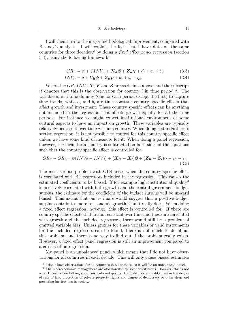
I will then turn to the major methodological improvement, compared withBleaney’s analysis. I will exploit the fact that I have data on the samecountries for three decades,2 by doing a fixed effect panel regression (section5.3), using the following framework:

GRit “ α ` ψINVit `Xitβ `Zitγ ` dt ` ai ` εit (3.3)INVit “ δ ` Vitφ`Zitρ` dt ` bi ` ηit (3.4)

Where the GR, INV ,X, V and Z are as defined above, and the subscriptit denotes that this is the observation for country i in time period t. Thevariable dt is a time dummy (one for each period except the first) to capturetime trends, while ai and bi are time constant country specific effects thataffect growth and investment. These country specific effects can be anythingnot included in the regression that affects growth equally for all the timeperiods. For instance we might expect institutional environment or somecultural aspects to have an impact on growth. These variables are typicallyrelatively persistent over time within a country. When doing a standard crosssection regression, it is not possible to control for this country specific effectunless we have some kind of measure for it. When doing a panel regression,however, the mean for a country is subtracted on both sides of the equationssuch that the country specific effect is controlled for:

GRit ´ĚGRi “ ψpINVit ´ ĘINV iq ` pXit ´ X̄iqβ ` pZit ´ Z̄iqγ ` εit ´ ε̄i(3.5)

The most serious problem with OLS arises when the country specific effectis correlated with the regressors included in the regression. This causes theestimated coefficients to be biased. If for example high institutional quality3is positively correlated with both growth and the central government budgetsurplus, the estimate for the coefficient of the budget surplus will be upwardbiased. This means that our estimate would suggest that a positive budgetsurplus contributes more to economic growth than it really does. When doinga fixed effect regression, however, this effect is controlled for. If there arecountry specific effects that are not constant over time and these are correlatedwith growth and the included regressors, there would still be a problem ofomitted variable bias. Unless proxies for these variables or valid instrumentsfor the included regressors can be found, there is not much to do aboutthis problem, and there is no way to find out if the problem really exists.However, a fixed effect panel regression is still an improvement compared toa cross section regression.

My panel is an unbalanced panel, which means that I do not have obser-vations for all countries in each decade. This will only cause biased estimates

2 I don’t have observations for all countries in all decades, so it will be an unbalanced panel.3 The macroeconomic management are also handled by some institutions. However, this is not

what I mean when talking about institutional quality. By institutional quality I mean the degreeof rule of law, protection of private property rights and degree of democracy or other deep andpersisting institutions in society.

3. Methodology 16

if there is a systematic reason for the variables to be unobserved that cor-relates with both groth and the regressors. I have not been able to detectsuch systematic explanations to why data is missing for countries, but it isnot impossible that there is one. However, if i were to use a balanced panel, Iwould be left with very few observations. To see which countries are includedin which decade, see Tab. 10 in Appendix B.

When doing growth analyses based on panel regressions there is a dilemmabetween setting the time period short to get as many observations as possible,and keeping the periods long enough to measure what you want to measure.Having many observations is good to make more accurate estimates, by keep-ing the standard errors down. But if I want to say something about howmacroeconomic management affects growth in the long term, I cannot basethe regression on, say, 3-year averages. Short period growth rates will beheavily influenced by short term macroeconomic fluctuations. I have cho-sen to base the regression on 10-year averages. This is long enough to notbe very biased by cyclical fluctuations but short enough to give me enoughobservations to keep the standard errors down.

3.3 Endogeniety of the investment rate

As mentioned in section 2.2 it might be argued that the investment ratedepends on the actual or expected growth rate of GDP. If this is the case,the model will be misspecified and the estimates suffer from a simultaneitybias. Bleaney mentiones this possibility (in a footnote), but states that "theexistence of simultaneous equation bias was rejected in a Hausman test, andthe equations were estimated by OLS." (Bleaney, 1996, p. 469). He is notexplicit about what instruments he used to perform the test, but if he basedthe test on the basic growth equation, the possible instruments are populationgrowth and initial GDP. These variables have very low explanatory power forgrowth (R2 “ 0.04), and according to Hahn et al. (2011) this causes theHausman test to be invalid. Unless we find stronger instruments for growth,there is no way we can be sure that growth is exogenous to the investmentrate. In the absence of good instruments it is also impossible to consistentlyestimate the equations in a simultaneous equation system.

Even though I find it little convincing that the investment rate is exoge-nous to growth, I have not been able to find good instruments, or in othersophisticated ways estimate these equations consistently. Doing so would be amethodological improvement, but it is simply too time consuming to be pos-sible in this thesis. I will therefore stick to the framework used by Bleaney(1996), extended by panel regressions.

4. MEASURING THE QUALITY OF MACROECONOMICMANAGEMENT

In order to assess the effect of macroeconomic management on economicgrowth it is necessary to find a convincing measure of how well countrieshandle their macroeconomic management. By good macroeconomic manage-ment I mean an economy where the government manages to provide a stablemacroeconomic environment, as defined in chapter 2.

Kormendi and Meguire (1985) were among the first to include macroeco-nomic policy variables in growth regressions. They found that the standarddeviation of unanticipated monetary growth was significantly negatively cor-related with growth in GDP for a sample of 47 countries over the period1950-77.

Both Cottani et al. (1990) and Dollar (1992) find real exchange rate vari-ability to be significantly negatively correlated to growth, and Cottani et al.(1990) also concludes that it is negatively correlated with investments. Ghuraand Grennes (1993) finds real exchange rate instability to be significantlynegatively correlated with investments, but not with growth, in a study of 33sub-Saharan African countries.

Fischer (1993) uses the inflation rate, the central government budget sur-plus/deficit and the black market exchange rate premium as indicators of thequality of the macroeconomic management. He argues that the inflation rateis the best indicator of how well a country manages its economy. It is widelyaccepted that very high inflation rates inhibit an efficient resource allocationand depress investment rates (Fischer, 1993, p. 487). Even though mostcountries aim for a positive inflation rate, there are no good arguments forvery high inflation rates. Therefore high inflation rates may be interpretedas an indication that the government has lost control over the economy.

Some countries manage to keep the inflation rate low and stable for along time, in an unsustainable way, for example by pegging their currencyto a major currency who’s economy is in a completely different situation.According to Fischer (1993, p. 487) these countries will most likely face fiscalor balance of payments problems, and the central government budget surplusor deficit will be a good indicator of such an unsustainable situation. As ameasure of the sustainability and appropriateness of the exchange rate, heuses the black market exchange rate premium.

Bleaney (1996) chose to focus on four concepts; the inflation rate, thestability of the real exchange rate, the budget balance and the (external) gov-ernment debt. More specifically, he used the five following indicators:

4. Measuring the quality of macroeconomic management 18

BS - the central government budget surplus (including grants) as percentageof GDP.

SDRER - the standard deviation of the logarithm of the real exchange rate.4

CPINFL - average consumer price inflation over the period 1980-90 (valueset to 100 % if average inflation exceeded that level).

DEBT79 - ratio of end-1979 foreign debt5 to 1979 export revenues.

HIC - a dummy variable that equals 1 if the country was classified as a highlyindebted country by the World Bank in 1989, and 0 otherwise.6

In theory it is primarily variability and thus uncertainty in the inflationrate that inhibits growth (see chapter 2), and ideally the variability of theinflation rate would be a good measure for this. In practice the variance andmean values of the inflation rates are so highly correlated (see Tab. 1), thatit is hard to distinguish the effects from one another in a regression. Bleaney(1996) therefore chooses to look at average inflation, and not the standarddeviation.

Tab. 1: Correlation between mean and standard deviation of inflation rate

sd(CPinf) mean(CPinf)sd(CPinf) 1.0000mean(CPinf) 0.9610 1.0000

In his sample, there are some countries that experienced extremely highinflation rates in some years. In order to avoid that these few observationsdetermine the coefficient estimate, a maximum of 100 % was imposed on theaverage inflation rate (Bleaney, 1996, p. 466).

Bleaney (1996, p. 466) argues that the central government budget sur-plus/deficit as percentage of GDP serves as a measure of the quality of fiscalmanagement. Though Keynesians would argue that running a deficit duringperiods of economic stagnation is a good way to stimulate the economy andthus create macroeconomic stability, this argument does not hold when look-ing at an 11-year average. The initial level of government debt essentiallymeasures the same thing as the budget surplus, but it measures how fiscalpolicy was handled in the past rather than at the present.

Bleaney (1996) uses the standard deviation of the logarithm of the realeffective exchange rate as a measure of the variability of the real exchangerate. Understanding how to interpret this variable is important in order toassess its importance for growth, when looking at the size of its coefficient

4 Where it was possible it was calculated from the real effective exchange rate as published inIMF International Financial Statistics, and otherwise from the bilateral consumer price based rateagainst the US dollar.

5 Government debt to foreign creditors.6 In this sample these were: Argentina, Bolivia, Chile, Colombia, Costa Rica, Ecuador, Morocco,

Ecuador, Mexico, Peru, Philippines, Uruguay and Venezuela (Bulow and Rogoff, 1990, p. 31).

4. Measuring the quality of macroeconomic management 19

estimates in chapter 5. Since this is only to get a vague idea about what thevalue of the variable means, we can think of the standard deviation as theaverage deviation from the mean:

SDRER “ sdplnpRERqq «

řTt“1 lnpRERtq ´ lnpĘRERq

T

And since lnpRERtq ´ lnpĘRERq « RERt´ĞRERĞRER

, we can think of SDRER asapproximately the real exchange rate’s average relative deviation from itsmean, i.e. SDRER=0.1 means that the real exchange rate had an averagerelative deviation from its mean of approximately 10 %. This sure is a measureof the predictability of the exchange rate, but it does not measure if theexchange rate is competitive or appropriate. If he also wanted to test this,he could use the black market premium, as in Fischer (1993). However I didnot find easily available data for enough countries to include this variable.

I have chosen to use the same indicators as Bleaney (1996), with somesmall differences. Due to lack of available data on foreign debt, I have chosento use total government debt as percentage of GDP instead of foreign debtas percentage of exports. Except from the regression where I replicate hisresults, I will not use the HIC dummy. This is because the World Bank doesnot have a list of countries classified as "highly indebted countries" anymore.Instead the World Bank, together with the IMF, have classified a number ofcountries as "highly indebted poor countries" (HIPC), which means that inaddition to being highly indebted, a country also has to be sufficiently poorto be labeled a HIPC. Including a HIPC dummy as a regressor would havecaused serious exogeneity problems, because being a poor country is a resultof having low growth. However the already included debt to GDP ratio is agood measure of how highly indebted the country is, so another measure ofthis is not really needed. The variables for inflation rate, budget surplus andexchange rate variability are constructed in the exact same way as in Bleaney(1996):

BS - the central government budget surplus (including grants) as percentageof GDP.

SDRER - the standard deviation of the logarithm of the real exchange rate.7

CPinf - average consumer price inflation over the period 1980-90 (value setto 100 % if average inflation exceeded that level).

debtX9 - ratio of end-1979 central government debt to 1979 GDP, for the1980s, and the same ratio for 1989 and 1999 for respectively the 1990sand 2000s.

7 Where it was possible it was calculated from the real effective exchange rate as published inIMF International Financial Statistics, and otherwise from the bilateral consumer price based rateagainst the US dollar.

5. RESULTS

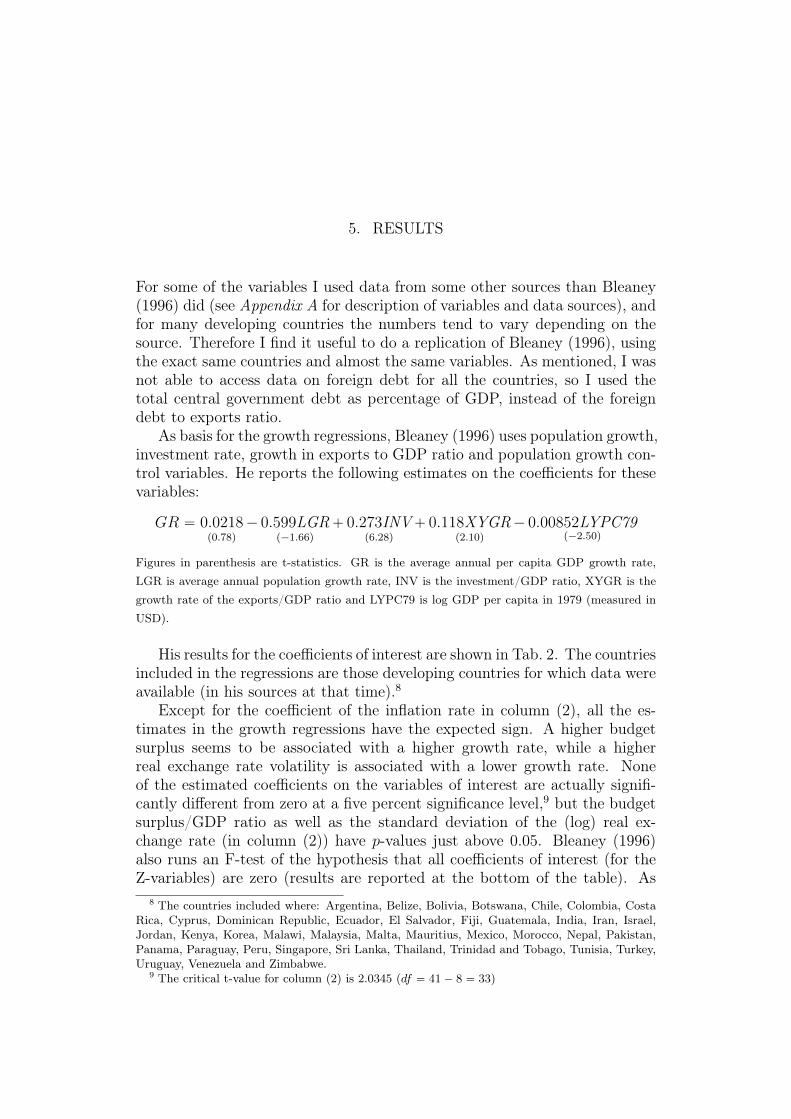
For some of the variables I used data from some other sources than Bleaney(1996) did (see Appendix A for description of variables and data sources), andfor many developing countries the numbers tend to vary depending on thesource. Therefore I find it useful to do a replication of Bleaney (1996), usingthe exact same countries and almost the same variables. As mentioned, I wasnot able to access data on foreign debt for all the countries, so I used thetotal central government debt as percentage of GDP, instead of the foreigndebt to exports ratio.

As basis for the growth regressions, Bleaney (1996) uses population growth,investment rate, growth in exports to GDP ratio and population growth con-trol variables. He reports the following estimates on the coefficients for thesevariables:

GR “ 0.0218p0.78q

´ 0.599LGRp´1.66q

` 0.273INVp6.28q

` 0.118XYGRp2.10q

´ 0.00852LYPC79p´2.50q

Figures in parenthesis are t-statistics. GR is the average annual per capita GDP growth rate,LGR is average annual population growth rate, INV is the investment/GDP ratio, XYGR is thegrowth rate of the exports/GDP ratio and LYPC79 is log GDP per capita in 1979 (measured inUSD).

His results for the coefficients of interest are shown in Tab. 2. The countriesincluded in the regressions are those developing countries for which data wereavailable (in his sources at that time).8

Except for the coefficient of the inflation rate in column (2), all the es-timates in the growth regressions have the expected sign. A higher budgetsurplus seems to be associated with a higher growth rate, while a higherreal exchange rate volatility is associated with a lower growth rate. Noneof the estimated coefficients on the variables of interest are actually signifi-cantly different from zero at a five percent significance level,9 but the budgetsurplus/GDP ratio as well as the standard deviation of the (log) real ex-change rate (in column (2)) have p-values just above 0.05. Bleaney (1996)also runs an F-test of the hypothesis that all coefficients of interest (for theZ-variables) are zero (results are reported at the bottom of the table). As

8 The countries included where: Argentina, Belize, Bolivia, Botswana, Chile, Colombia, CostaRica, Cyprus, Dominican Republic, Ecuador, El Salvador, Fiji, Guatemala, India, Iran, Israel,Jordan, Kenya, Korea, Malawi, Malaysia, Malta, Mauritius, Mexico, Morocco, Nepal, Pakistan,Panama, Paraguay, Peru, Singapore, Sri Lanka, Thailand, Trinidad and Tobago, Tunisia, Turkey,Uruguay, Venezuela and Zimbabwe.

9 The critical t-value for column (2) is 2.0345 (df “ 41´ 8 “ 33)

5. Results 21

Tab. 2: The original results in Bleaney (1996)

(I) (2) (3) (4) (5) (6) Dependent variable: PCGR PCGR PCGR INV INV INV Coefficient of

BS 0.155 0.164 0.386 0.337 0.362 (1.78) (2.01) (1.52) (1.45) (1.54)

SDRER (X 10- 2 ) -4.42 -6.91 -8.86 -1.90 -10.08 ( - 1.29) ( - 2.03) ( -0.89) (-0.19) ( - 1.35)

CPINFL (X 10- 4 ) -0.501 0.399 -1.96 -0.584 ( -0.36) (0.33) ( -0.47) (-0.14)

DEB179 ( X 10- 2) -0.145 0.273

( -0.75) (0.50) HIC -0.043 -3.65

(-0.05) ( - 1.75) INV* BS 0.631

(1.95) INV* SDRER (X 10- 2 ) -2.39

( - 1.45) INV* PINFL (X 10- 4 ) -0.441

( -0.60) INV* DEB179 ( X 10- 2

) -0.588 (-0.69)

F-statistic 2.29 1.94 3.55 0.88 1.66 1.62 [marginal significance] [0.08] [0.13] [0.02] [0.49] [0.18] [0.21] n 40 41 40 39 39 39

Figures in parentheses are t-statistics. Additional regressors included are those shown in preferred regres-

sions given in the text. PCGR - average annual per capita GDP growth rate; INV - investment/GDP

ratio; BS - average central government budget surplus (% GDP); SDRER - standard deviation of log(real

exchange rate); CPINFL - average annual inflation rate (truncated at 100%); DEBT79 - ratio of external

debt to exports in 1979; HIC - dummy variable = 1 for highly indebted country in 1989. F-statistic is a

test of the hypothesis that coefficients of regressors shown are jointly zero.

Source: Bleaney (1996)

we see, the hypothesis is rejected at a 10 % significance level for two of thegrowth regressions. This is a fairly strong indication that there actually is arelationship between these four indicators of macroeconomic (in)stability andeconomic growth.

I will come back to the issue of economic significance in chapter 6, butit’s worth to take a look at the size of the coefficient estimates for BS andSDRER. If we use the estimates in column (2), we see that a decrease inthe average budget deficit (increase in the average budget surplus) with onepercentage point of GDP is associated with an increase of 0.164 percentagepoints in the average growth rate. Put differently, an increase in averagebudget surplus of six percentage points of GDP is associated with an increaseof one percentage point in average growth rate.

Interpreting the coefficient of SDRER is a bit harder. Recall that if weinterpret the standard deviation as roughly the average deviation from themean, and remember that the difference between the logarithm of two values

5. Results 22

is approximately the relative change in the value, we can interpret SDRERas the real exchange rate’s average relative deviation from its mean. Tomake it clearer; a one unit increase in SDRER means that the real exchangerate’s average relative deviation from its mean increases by 100 percentagepoints. The estimate tells us that an increase in the standard deviation ofthe real exchange rate by 1 is associated with a 6.9 percentage point decreasein the average growth rate.10 Or put differently, that an increase in the realexchange rate’s average relative deviation from its mean by 10 percentagepoints is associated with a 0.69 percentage points drop in growth rate. Takeninto account that 95 percent of the observations in my sample has a value ofSDRER of 0.36 or below (the values range from 0.01 to 3.9511), a change of0.1 is quite a large change. But for countries with very high real exchangerate volatility, there might be a lot to gain from reducing this volatility, if thepoint estimate should be taken seriously.

With regard to the theory discussed in chapter 2, one of the most interest-ing findings is that when the investment rate is controlled for, macroeconomicstability seems to matter for economic growth, but it is far less clear that itmatters for investments. I will discuss possible explanations for this in chap-ter 6.

5.1 Replication of Bleaney (1996)

In this section I will use the same method and the same countries as Bleaney(1996), but not all my data are from the same sources as his. As mentionedin chapter 4, Bleaney uses the foreign debt of the central government aspercentage of exports whereas I use the total central government debt aspercentage of GDP. Other than that, all variables are constructed in thesame way.

The estimated coefficients on the control variables are, with one exception,very similar to those of Bleaney (1996):

GR “ 0.0472p1.52q

´ 0.941LGRp´2.52q

` 0.283INVp4.68q

` 0.114XYGRp1.43q

´ 0.00963LYPC79p´2.61q

Figures in parenthesis are t-statistics. The variables are the same as above

The coefficient estimate of the impact of population growth on per capitaGDP growth, is considerably larger here than in Bleaney (1996). I have triedpopulation data from several different databases12 and they all yield more orless the same result. Given that the other coefficient estimates are similarto the ones in Bleaney (1996), the most plausible explanation is that he hadpoor data on population growth.13

10 The rates are expressed in decimals, so the coefficient of SDRER must be multiplied by 100.11 There are only two observations in my sample with values of SDRER above one. Excluding

these from the sample has no significant effect on any of the estimates.12 The World Bank’s WDI, IMF’s IFS and Penn World Table.13 I have been in touch with Prof. Bleaney, and he confirms that I have constructed the variables

correctly, but he no longer has the dataset, so it is hard to find out what causes this difference.

5. Results 23

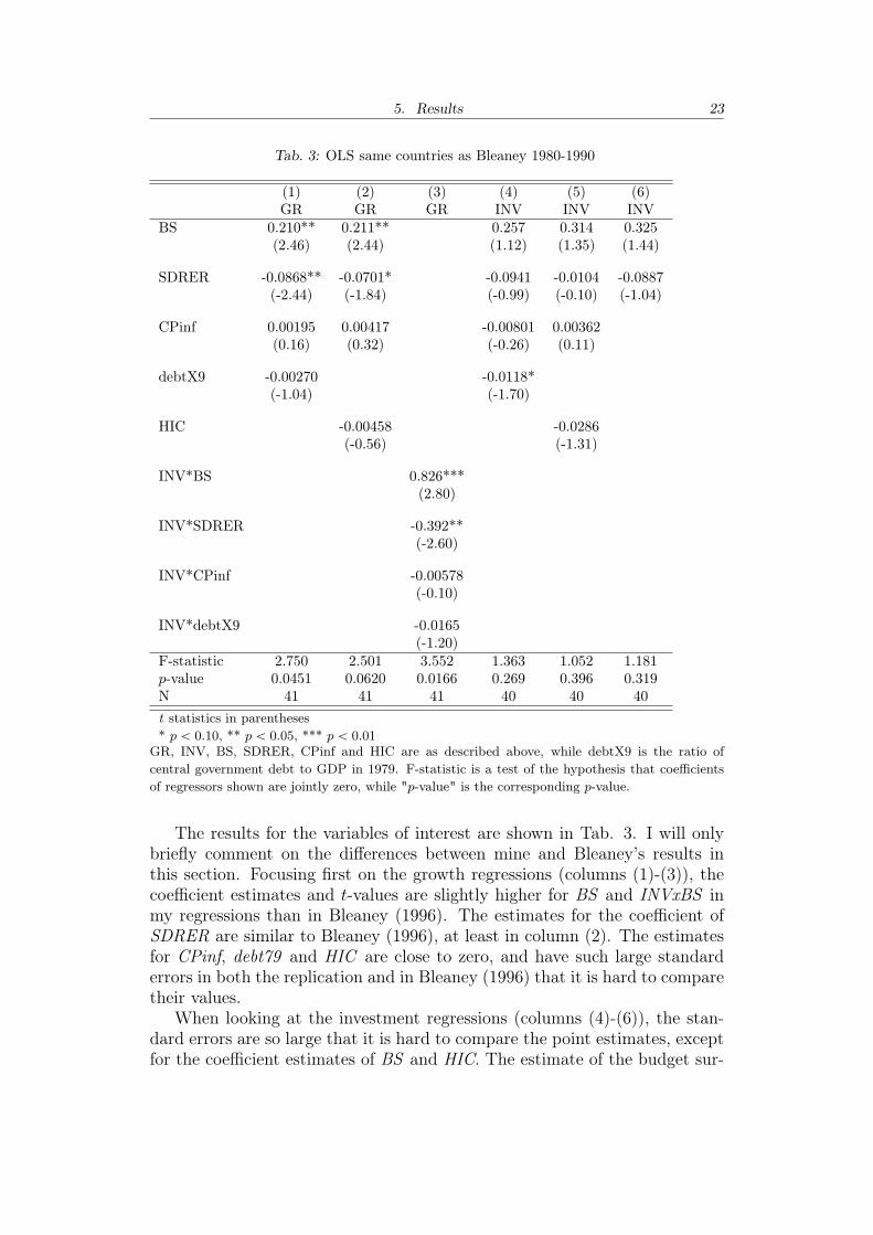
Tab. 3: OLS same countries as Bleaney 1980-1990

(1) (2) (3) (4) (5) (6)GR GR GR INV INV INV

BS 0.210** 0.211** 0.257 0.314 0.325(2.46) (2.44) (1.12) (1.35) (1.44)

SDRER -0.0868** -0.0701* -0.0941 -0.0104 -0.0887(-2.44) (-1.84) (-0.99) (-0.10) (-1.04)

CPinf 0.00195 0.00417 -0.00801 0.00362(0.16) (0.32) (-0.26) (0.11)

debtX9 -0.00270 -0.0118*(-1.04) (-1.70)

HIC -0.00458 -0.0286(-0.56) (-1.31)

INV*BS 0.826***(2.80)

INV*SDRER -0.392**(-2.60)

INV*CPinf -0.00578(-0.10)

INV*debtX9 -0.0165(-1.20)

F-statistic 2.750 2.501 3.552 1.363 1.052 1.181p-value 0.0451 0.0620 0.0166 0.269 0.396 0.319N 41 41 41 40 40 40t statistics in parentheses* p ă 0.10, ** p ă 0.05, *** p ă 0.01

GR, INV, BS, SDRER, CPinf and HIC are as described above, while debtX9 is the ratio ofcentral government debt to GDP in 1979. F-statistic is a test of the hypothesis that coefficientsof regressors shown are jointly zero, while "p-value" is the corresponding p-value.

The results for the variables of interest are shown in Tab. 3. I will onlybriefly comment on the differences between mine and Bleaney’s results inthis section. Focusing first on the growth regressions (columns (1)-(3)), thecoefficient estimates and t-values are slightly higher for BS and INVxBS inmy regressions than in Bleaney (1996). The estimates for the coefficient ofSDRER are similar to Bleaney (1996), at least in column (2). The estimatesfor CPinf, debt79 and HIC are close to zero, and have such large standarderrors in both the replication and in Bleaney (1996) that it is hard to comparetheir values.

When looking at the investment regressions (columns (4)-(6)), the stan-dard errors are so large that it is hard to compare the point estimates, exceptfor the coefficient estimates of BS and HIC. The estimate of the budget sur-

5. Results 24

plus coefficient is more or less the same, while the HIC coefficient estimateis much lower in the replication than in Bleaney (1996).

By looking at the joint significance tests, we see the same observation asin Bleaney (1996), namely that it seems like there is a relationship betweenthe indicators of macroeconomic stability and per capita GDP growth, butthere is no evidence that there is a relationship between these indicators andthe investment rate.

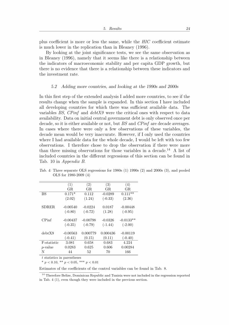
5.2 Adding more countries, and looking at the 1990s and 2000s

In this first step of the extended analysis I added more countries, to see if theresults change when the sample is expanded. In this section I have includedall developing countries for which there was sufficient available data. Thevariables BS, CPinf and debtX9 were the critical ones with respect to dataavailability. Data on initial central government debt is only observed once perdecade, so it is either available or not, but BS and CPinf are decade averages.In cases where there were only a few observations of these variables, thedecade mean would be very inaccurate. However, if I only used the countrieswhere I had available data for the whole decade, I would be left with too fewobservations. I therefore chose to drop the observation if there were morethan three missing observations for those variables in a decade.14 A list ofincluded countries in the different regressions of this section can be found inTab. 10 in Appendix B.

Tab. 4: Three separate OLS regressions for 1980s (1) 1990s (2) and 2000s (3), and pooledOLS for 1980-2009 (4)

(1) (2) (3) (4)GR GR GR GR

BS 0.171* 0.112 -0.0289 0.111**(2.02) (1.24) (-0.33) (2.36)

SDRER -0.00540 -0.0224 0.0187 -0.00448(-0.80) (-0.72) (1.28) (-0.95)

CPinf -0.00437 -0.00798 -0.0326 -0.0133**(-0.35) (-0.79) (-1.44) (-2.00)

debtX9 -0.00563 0.000779 0.000436 -0.00119(-0.41) (0.15) (0.11) (-0.40)

F-statistic 3.081 0.658 0.683 4.224p-value 0.0283 0.625 0.606 0.00284N 44 52 70 166t statistics in parentheses* p ă 0.10, ** p ă 0.05, *** p ă 0.01

Estimates of the coefficients of the control variables can be found in Tab. 8.14 Therefore Belize, Dominican Republic and Tunisia were not included in the regression reported

in Tab. 4 (1), even though they were included in the previous section.

5. Results 25

The results for the years 1980-89 are shown in Tab. 4 (1). We see twonoticeable differences between this and the results in the previous section. Thecoefficient of BS is somewhat lower, and the coefficient of SDRER is muchlower and insignificant. I will investigate this result further in section 6.1.The coefficients for inflation and initial government debt remain low andinsignificant. What is also worth noticing is that the hypothesis that all ofthem are zero is rejected at a very low level of significance (p-value of 0.02).This strengthens the hypothesis that macroeconomic stability matters forgrowth.

When looking at the results for the 1990s (column (2)), we see that thecoefficient of the budget surplus is even lower and insignificant. None of thevariables seems to be significant alone, and even the joint significance testcannot reject the hypothesis that all coefficients are zero.

The results for the 2000s in column (3) differ from the 1980s in many in-teresting aspects. Firstly the estimate of the coefficient of the inflation rate isnotably larger (in absolute value) and its t-value is also higher. Secondly thecoefficient of SDRER is positive, which is the opposite of what we would ex-pect from theory, but still statistically insignificant. The coefficient estimateof the budget surplus is very close to zero (even negative) and statisticallyinsignificant. Why this estimate differs so much from the others will also bediscussed in section 6.1. To test if any of the coefficient estimates for the 1990sand 2000s were significantly different from the estimates for the 1980s, I rana pooled OLS regression with dummies for the 1990s and 2000s multipliedwith each of the regressors. The results showed that none of the estimateswere significantly different from each other at a five percent significance level.Another thing worth noticing is that the joint hypothesis test does not rejectthe hypothesis that all coefficients equal zero.

Column (4) shows the results from a pooled OLS regression, with dummiesfor the 1990s and 2000s, to control for time trends. The coefficient of theinflation rate is negative and significant at a five percent level, but the impactseems to be very small. The coefficient of the budget surplus is lower thanin the 1980s regression, but still statistically significant. I will come backto discussing this finding in section 6.1. What is also worth noticing is thatalthough the joint significance tests for the 1990s and 2000s do not reject thehypothesis that all coefficients are zero, it is rejected at a very low significancefor the pooled OLS regression.

In this section I have expanded the analyses of section 5.1 and in Bleaney(1996) and looked at each decade separately. I have not taken advantage ofthe panel structure of the data, in order to control for time constant countryspecific effects. This is the topic for the next section.

5. Results 26

5.3 Panel regression

To be able to control for time constant country fixed effects like institutionalquality or cultural differences, I ran fixed effects panel regressions. The resultsof these regressions are shown in Tab. 5. There are several interesting things

Tab. 5: GDP per capita growth and investment on indicators of macroeconomic stability (panelregression)

(1) (2) (3) (4) (5)GR GR GR INV INV

BS 0.0202 0.0435 0.371 0.309(0.27) (0.52) (1.37) (1.22)

SDRER -0.00316 -0.00328 -0.00339 -0.000919(-0.55) (-0.57) (-0.16) (-0.05)

CPinf -0.0272*** -0.0202** 0.00402 -0.00716(-3.12) (-2.03) (0.12) (-0.24)

debtX9 -0.00974* -0.0142(-1.84) (-0.83)

INV*BS 0.125(0.36)

INV*SDRER -0.0137(-0.52)

INV*CPinf -0.117**(-2.41)

INV*DEBTX9 -0.0469**(-2.00)

F-statistic 5.134 3.076 3.727 0.736 0.720p-value 0.00275 0.0217 0.00842 0.570 0.543N 174 166 166 164 170t statistics in parentheses* p ă 0.10, ** p ă 0.05, *** p ă 0.01

Estimates of the coefficients of the control variables can be found in Tab. 9.

worth noticing about the results of the growth regressions (column (1)-(3)). Inthe growth regressions, the central government budget surplus seems to haveno effect on growth. The coefficient estimates are close to zero, and so are thet-values. This is in stark contrast to the findings of Bleaney (1996), wherethe budget surplus seems to be the most significant variable. The estimate ofreal exchange rate volatility coefficient is close to zero and insignificant. Thisis also very different from the results in Bleaney (1996), where it appeared asstatistically significant and of a size that suggested an economically significantimpact on the growth rate, at least for countries with high real exchange ratevolatility.

The inflation rate appears as statistically significant, with a coefficient

5. Results 27

estimate of around ´0.02 (in column (2)). This tells us that an increase inthe inflation rate by one percentage point is associated with a 0.02 percentagepoints decrease in the growth rate. Or equivalently that a decrease in theinflation rate by 10 percentage points is associated with a 0.2 percentagepoints increase in growth rate. This is much higher than the estimates inBleaney (1996), but it is still not enough to be regarded as economicallysignificant.

While the government debt to GDP ratio seems to be statistically signifi-cant at a 10 percent significance level, the coefficient estimate is so small thatit can be regarded as economically insignificant.

In Bleaney (1996) and in section 5.1, the specification where the Z vari-ables are multiplied with the investment rate (3) fits the data marginallybetter (the F-values are higher). Bleaney interprets this as an indication that"the impact of macroeconomic instability falls mainly on the quality of thecapital stock" (Bleaney, 1996, p. 471). By the quality of an investment, hemeans the return to the investment. A more stable macroeconomic environ-ment makes it easier to predict future demand and future earnings, thus itis more likely that the investment will ensure an allocation of resources thatmaximizes the value of production. The results in section 5.1 indicate thesame, but this is far less clear in the panel regression.

When looking at the investment regressions in the two last columns ofTab. 5, we see that the only variable that is somewhere close to significant isthe central government budget surplus as percentage of GDP. It is importantto keep in mind that budget deficits need to be financed through borrowing.The negative effect that budget deficits (maybe) have on the investment rate,might therefore be a result of a crowding out effect (see chapter 2).

Before moving on to discussing these findings, it is worth taking a lookat the joint significance tests. By looking at the F-statistics for the growthregressions, we see that the hypothesis that the coefficients of all the regres-sors of interest are zero is rejected at every reasonable level of significance.However, this is not the case for the investment regressions. This is the sameresult as in Bleaney (1996), and can be interpreted to strengthen the hypoth-esis that macroeconomic stability affects growth through other channels thanthe investment channel. Although the evidence for statistical significanceseems very strong, none of the indicators of macroeconomic stability seem tohave an impact on growth that is large enough to be regarded as economicallysignificant.

6. DISCUSSION

After expanding Bleaney’s (1996) analysis, first by adding more observationsand then by performing a panel regression, there are a few interesting findingsthat deserve some discussion. I will keep the discussion mainly to the growthregressions, since the investment regressions do not differ that much and sinceI do not have enough control variables in those regressions for the results tobe very reliable.

To start at the general level, the joint significance tests indicate that thereis a relationship between the indicators of macroeconomic (mis)managementand growth. In the panel regression, the hypothesis that all the coefficients ofthe Z variables are zero, is rejected at every reasonable level of significance.This is confirmed in section 5.2 by looking at the regression for the 1980s andthe pooled OLS regression. However, it is not rejected in the regressions forthe 1990s and the 2000s.

A second interesting finding is that the coefficient of the budget surplus,which is relatively large and significant in the 1980s regression, is very lowand insignificant in the OLS regressions for the other decades as well as inthe panel regression. It turns out that this can probably be explained by thefact that one single outlier with extraordinary high values on both budgetsurplus and growth in the 1980s is responsible for the size and significance ofthe coefficient. I will look into the issue of outliers in section 6.1.

A third thing worth noticing is that the coefficient on inflation has theexpected sign in all specifications in the panel regression. It is also alot largerthan in Bleaney (1996), and it is significant on a five percent level. Thismight be interpreted as an argument in favour of the hypothesis that highinflation inhibits growth, but it might also be a result of a spurious effect, asI will discuss in section 6.2. Although it is statistically significant, it does notseem to be economically significant. However, this might be a result of theway the equation is specified. I will look further into this in section 6.3.

Also the initial government debt as percentage of GDP seems to be neg-atively associated with economic growth, but the estimated coefficient is solow that huge reductions in the debt level are associated with very small im-provements in the growth rate. As with the investment rate, this might alsobe a result of the specification of the equation (see section 6.3).

After this extended analysis it is a somewhat confusing result that re-mains. When looking at the results from the panel regression (Tab. 5), thestatistical significance is stronger than what was demonstrated in Bleaney(1996), but the economic significance is weaker. The results from the panelregression strongly support the hypothesis that there exists a relationship

6. Discussion 29

between macroeconomic stability and growth, yet the size of the coefficientsare so small that it seems like very large improvements in the indicators ofmacroeconomic stability are associated with small increases in growth rates.The main reason for this is that the results from the panel regression donot support the hypothesis that a lower budget deficit is associated with ahigher growth rate. Nor do they support the hypothesis that real exchangerate volatility inhibits growth. These were the most significant (statisticallyand economic) variables in Bleaney’s analysis. The only two Z variables thatappear to be associated with growth are the inflation rate and the initialgovernment debt. And though they seem to be statistically significant, itseems like their impact on growth is so small that even large improvementsin these are associated with moderate improvements in growth rate, but asmentioned, this may be a result of how the model is specified.

Before I discuss potential problems with the results in the panel regressionI will discuss the concept of outliers, and look into how single outliers aredriving the results in Bleaney (1996), and can explain some of the differencesbetween the result in the panel regression and the cross section regressions insection 5.1.

6.1 Outliers

An outlier is an observation that does not seem to follow the pattern of theother data points. When doing OLS regressions with small samples, one hasto be aware of the effect an outlier has on the estimates. The same is truefor true for panel regressions, since it is only a modified form of OLS. Thedanger is that the outlier causes a bias in the coefficient estimate:

[A] large error when squared becomes very large, so when mini-mizing the sum of squared errors OLS gives a high weight to thisobservation, causing the OLS estimating line to swing towards thisobservation, masking the fact that it is an outlier.(Kennedy, 2009, p. 346).

This problem will be especially severe in small samples, like the ones used inthis paper.

To investigate whether there are outliers that are causing large biases inmy results the first task would be to identify the outliers. To do this for theOLS regressions, I plotted the estimated residuals against each variable ofinterest, to see if any of the observation differed much from the others. Asshown in Fig. 3, there is one country that has an average government budgetsurplus way above the other countries, that also has a high estimated residual,namely Botswana.

The next step would be to run the regression again without Botswana inthe sample. The results of this regression are shown in Tab. 6 (1). As wesee, the estimate of the coefficient of the budget surplus is less than half ofwhat it was in Tab. 3, and it is no longer significant. The same happens in

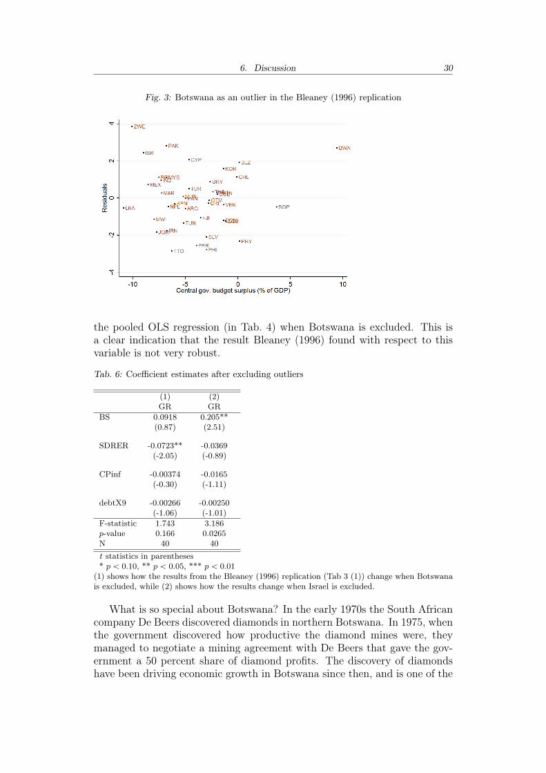
6. Discussion 30

Fig. 3: Botswana as an outlier in the Bleaney (1996) replication

the pooled OLS regression (in Tab. 4) when Botswana is excluded. This isa clear indication that the result Bleaney (1996) found with respect to thisvariable is not very robust.

Tab. 6: Coefficient estimates after excluding outliers

(1) (2)GR GR

BS 0.0918 0.205**(0.87) (2.51)

SDRER -0.0723** -0.0369(-2.05) (-0.89)

CPinf -0.00374 -0.0165(-0.30) (-1.11)

debtX9 -0.00266 -0.00250(-1.06) (-1.01)

F-statistic 1.743 3.186p-value 0.166 0.0265N 40 40t statistics in parentheses* p ă 0.10, ** p ă 0.05, *** p ă 0.01

(1) shows how the results from the Bleaney (1996) replication (Tab 3 (1)) change when Botswanais excluded, while (2) shows how the results change when Israel is excluded.

What is so special about Botswana? In the early 1970s the South Africancompany De Beers discovered diamonds in northern Botswana. In 1975, whenthe government discovered how productive the diamond mines were, theymanaged to negotiate a mining agreement with De Beers that gave the gov-ernment a 50 percent share of diamond profits. The discovery of diamondshave been driving economic growth in Botswana since then, and is one of the

6. Discussion 31

reasons why Botswana has been among the fastest growing countries for thelast 40 years. Due to the mining deal it has also contributed to giving thegovernment high budget surpluses (Acemoglu et al., 2002).

This is a clear example of an omitted variable (the presence of diamonds)that affects both the budget surplus and the growth rate, and causes a biasin the estimates. It also demonstrates how vulnerable regressions with fewobservations are to outliers like Botswana.

Looking at the residual plots may be a subjective way of finding potentialoutliers. It may also be hard to spot them, because the process of minimizingsquared residuals makes sure that the residuals are not so large. A moresystematic way of investigating this problem, is to run the regression n timeswhere observation i is excluded from the sample, one at a time (Kennedy,2009, p. 346–347). I used this method to control for outliers in all of theregressions in chapter 5. In addition to Botswana’s effect on the coefficientof the budget surplus, there was one other country that seemed to have asevere impact on an estimate, namely Israel. When Israel was excluded fromthe sample, the coefficient of SDRER became much smaller and insignificant(see Tab. 6 (2)).

Israel had a relatively stable real exchange rate in the 1980s despite veryhigh inflation in the start of the decade. They had a relatively low investmentrate, high initial GDP per capita and a negative growth in the exports/GDPratio. These are all factors that are associated with a low growth rate in myregressions, yet Israel had an average annual growth rate of 2 percent for theyears 1980-1990. An explanation to why Israel seems to be driving the resultcan be that it scores high on some omitted variable, like institutional quality,that contributes to a higher growth rate, but since it also had a stable realexchange rate it becomes an outlier that biases the estimate of the coefficientof SDRER.

We have seen that excluding some outliers may change the results dramat-ically. But are these results more reliable than the ones where the outliersare included? If the reason the outlier observations are outliers is becauseof measurement errors, the answer is clearly yes. If not, then it is less clearwhat to do about them (Kennedy, 2009, p. 346–347). They may be outliersbecause they simply do not fit the model. So excluding them would make themodel fit better to the data. However I will argue that this is not likely to bethe case here.

Excluding Botswana in the Bleaney (1996) replication does not make themodel fit the data better. On the contrary, we see that this single observationwas the reason why the budget surplus coefficient seemed to be statisticallysignificant. The same can be said about Israel and the real exchange ratevolatility coefficient.

The fact that the results for BS and SDRER are so sensitive to one singleobservation casts doubt on the robustness of the result. The observationthat when including more data and controlling for country fixed effect, theestimates turns out as insignificant, shows that we have good reason to doubt

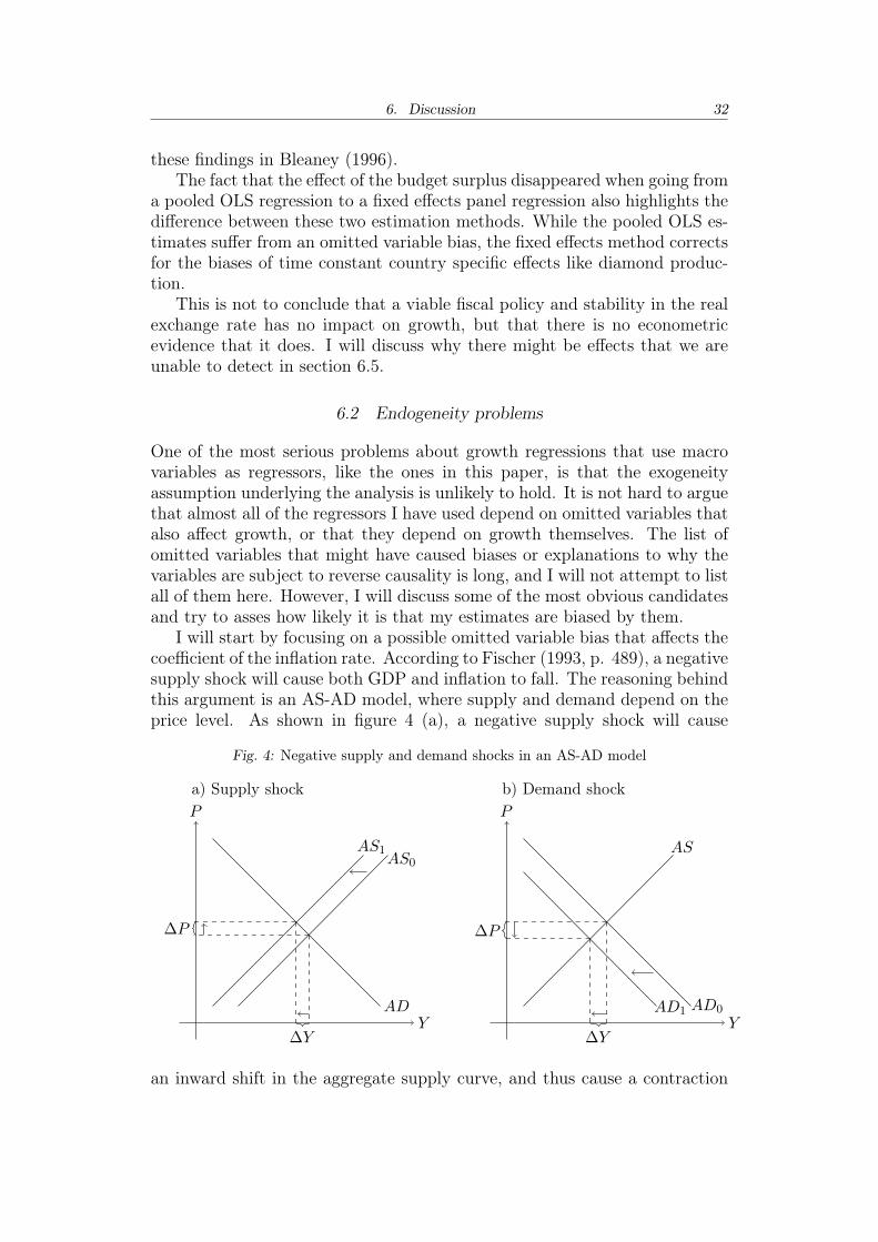
6. Discussion 32

these findings in Bleaney (1996).The fact that the effect of the budget surplus disappeared when going from

a pooled OLS regression to a fixed effects panel regression also highlights thedifference between these two estimation methods. While the pooled OLS es-timates suffer from an omitted variable bias, the fixed effects method correctsfor the biases of time constant country specific effects like diamond produc-tion.

This is not to conclude that a viable fiscal policy and stability in the realexchange rate has no impact on growth, but that there is no econometricevidence that it does. I will discuss why there might be effects that we areunable to detect in section 6.5.

6.2 Endogeneity problems

One of the most serious problems about growth regressions that use macrovariables as regressors, like the ones in this paper, is that the exogeneityassumption underlying the analysis is unlikely to hold. It is not hard to arguethat almost all of the regressors I have used depend on omitted variables thatalso affect growth, or that they depend on growth themselves. The list ofomitted variables that might have caused biases or explanations to why thevariables are subject to reverse causality is long, and I will not attempt to listall of them here. However, I will discuss some of the most obvious candidatesand try to asses how likely it is that my estimates are biased by them.

I will start by focusing on a possible omitted variable bias that affects thecoefficient of the inflation rate. According to Fischer (1993, p. 489), a negativesupply shock will cause both GDP and inflation to fall. The reasoning behindthis argument is an AS-AD model, where supply and demand depend on theprice level. As shown in figure 4 (a), a negative supply shock will cause

Fig. 4: Negative supply and demand shocks in an AS-AD model

a) Supply shock b) Demand shock

AS0AS1

ADY

P

∆P

∆Y

AS

AD0AD1Y

P

∆P

∆Y

an inward shift in the aggregate supply curve, and thus cause a contraction

6. Discussion 33

in GDP and an increase in the price level. However, a negative demandshock would cause a contraction in GDP and a decrease in the price level(see Fig. 4 (b)). If these kinds of shocks have large impacts on 10 yearaverage growth and inflation rates, which way they bias the coefficient dependon whether supply shocks or demand shocks are most common. If demandshocks are most common, it might be that my estimate on the coefficientof the inflation rate is upward biased (too low in absolute value). However,unless these shocks are very large and persistent, it is not very likely thatthey contribute to any large biases.

Due to the way the real exchange variable is constructed (R “ P˚EP

) a highinflation rate will automatically cause the real exchange rate to appreciate.This might be offset by a nominal depreciation, but in practice (at leastin my dataset) we see that the correlation between inflation rate and realexchange rate volatility is high, which is an indication that these usually donot perfectly offset each other. This means that if the presence of supplyor demand shocks biase the coefficient estimates of the inflation rate, it willalso bias the SDRER coefficient estimate. While positive and negative shockshave opposite effects on the growth rate, they will both contribute to a higherexchange rate volatility. Hence, whether it is upward or downward biaseddepends on whether positive or negative supply and demand shocks are mostcommon. However, since the coefficient estimate is so low and insignificant,I will not spend more time discussing this possibility.

The government debt to GDP ratio will naturally depend on the size ofGDP and thus the growth rate. This is the reason why I have used theinitial level, meaning the year before the decade started. There is no waythat growth in the 1980s could affect the ratio of government debt to GDPin 1979. However, a low growth rate in the 1970s may have contributed to alarge debt to GDP ratio in 1979. This is both because it contributes to a lowerGDP in 1979, because the low growth may have generated less income for thegovernment and thus led to larger budget deficits and because countries withlow growth faced higher interest rates because of higher default risk. If therewas some variable that reduced growth in the 1970s that also had the sameeffect on growth in the 1980s, this variable indirectly caused a high initial debtto GDP ratio as well as low growth in the 1980s. However, such a variableshould be persistent over time, and these kinds of variables are controlled forin the fixed effect panel regressions.

The central government budget surplus is likely to be high in years ofeconomic expansion and low in years of economic contraction. Including thisvariable in a growth regression should therefore be done with great care. Theargument for exogeneity to hold is that we are looking at 10 year averages,and that cyclical effects will be canceled out over this period. However, aswe have seen in the case of Botswana, there might be omitted variables thatcause high growth for more than a decade and gives the government additionalincome which causes high budget surpluses. Also here, we would expect sucha variable to be relatively persistent over time, so this problem will be smaller

6. Discussion 34

in a fixed effect panel regression than in the cross country regression. Thefact that the budget surplus seems to be insignificant in the panel regression,even though Botswana is included, is a good example of this.

6.3 Specification

The results from the panel regression indicate that the investment rate andthe initial level of government debt are significantly correlated to the growthrate, but that the impact is so low that even very large improvements on thesewill have small effects on the growth rate. However, it might be too soon toconclude that these two variables have no economically significant impacton growth. One possibility is that government debt and inflation have noimpact on growth as long as they are at moderate levels, but when they crossa threshold it becomes detrimental to economic growth.

Reinhart and Rogoff (2010) showed that government debt have no sig-nificant impact on growth until it reaches 90 percent of GDP. Above thisthreshold, there is a sharp drop in growth rates.15 A reasoning behind thismay be that it is only when the debt reaches a certain level that the actorsperceive it as unsustainable, and they realize that the government may beunable to repay.

A similar argument can be made with respect to the inflation rate: Atmoderate levels of inflation there is certainty about future price levels, and itmight not have any impact on economic growth. It is only when the inflationrate reaches a certain level that it becomes detrimental to growth. It is alsopossible to argue that as long as it is above this level it does not matter howhigh the inflation is, because above this threshold the price as an informationmechanism has ceased to function.

To check if a threshold model, where debt and inflation has no impactat moderate levels, but has a negative impact on growth when it reaches acertain level, I generated dummy variables. One dummy that equals one if theinitial government debt to GDP ratio is above 90 percent and zero otherwiseand one that equals one if the average rate of inflation is above 25 percentand zero otherwise. These were included in the panel regression instead ofthe original inflation and debt variables.

Of the 166 observations there were 20 that had initial government debtlevel above 90 percent of GDP, their per capita GDP growth rate averaged1.7 percent, while the 146 observations that had initial government debt ofless than 90 percent had an average growth rate of 2.5 percent. There were 20observations with average inflation above 25 percent. Their average annualgrowth rate was 0.7 percent, while the average growth rate for the 146 ob-servations with moderate inflation rates was 2.6 percent. For the rest of the

15 Thomas Herndon, Michael Ash and Robert Pollin of the University of Massachusetts discov-ered a coding error in the excel spreadsheet of Reinhart and Rogoff (2010) that caused these resultsto be biased. However, Reinhart and Rogoff argue that this was just one of several calculations,and that their main result still holds (The Economist, 2013).

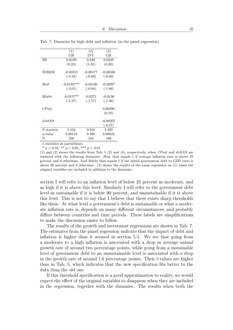
6. Discussion 35

Tab. 7: Dummies for high debt and inflation (in the panel regression)

(1) (2) (3)GR INV GR

BS 0.0189 0.349 0.0249(0.24) (1.31) (0.30)

SDRER -0.00315 -0.00177 -0.00336(-0.58) (-0.09) (-0.60)

Hinf -0.0194*** -0.00100 -0.0209*(-3.01) (-0.04) (-1.86)

Hdebt -0.0157** -0.0271 -0.0136(-2.37) (-1.17) (-1.36)

CPinf 0.00296(0.18)

debtX9 -0.00207(-0.27)

F-statistic 5.102 0.916 3.320p-value 0.00118 0.460 0.00643N 166 164 166t statistics in parentheses* p ă 0.10, ** p ă 0.05, *** p ă 0.01

(1) and (2) shows the results from Tab. 5 (2) and (4), respectively, when CPinf and debtX9 arereplaced with the following dummies: Hinf, that equals 1 if average inflation rate is above 25percent and 0 otherwise. And Hdebt, that equals 1 if the initial government debt to GDP ratio isabove 90 percent and 0 otherwise. (3) shows the results of the same regression as (1) when theoriginal variables are included in addition to the dummies.

section I will refer to an inflation level of below 25 percent as moderate, andas high if it is above this level. Similarly I will refer to the government debtlevel as sustainable if it is below 90 percent, and unsustainable if it is abovethis level. This is not to say that I believe that there exists sharp thresholdslike these. At what level a government’s debt is sustainable or what a moder-ate inflation rate is, depends on many different circumstances, and probablydiffers between countries and time periods. These labels are simplificationsto make the discussion easier to follow.

The results of the growth and investment regressions are shown in Tab. 7.The estimates from the panel regression indicate that the impact of debt andinflation is higher than it seemed in section 5.3. We see that going froma moderate to a high inflation is associated with a drop in average annualgrowth rate of around two percentage points, while going from a sustainablelevel of government debt to an unsustainable level is associated with a dropin the growth rate of around 1.6 percentage points. Their t-values are higherthan in Tab. 5, which indicates that the new specification fits better to thedata than the old one.

If this threshold specification is a good approximation to reality, we wouldexpect the effect of the original variables to disappear when they are includedin the regression, together with the dummies. The results when both the

6. Discussion 36

dummies and their original variables are included in the regression are shownin column (3). None of them are significant at a five percent level, but thet-values of CPinf and debtX9 are close to zero, while the t-values of Hinf andHdebt are -1.86 and -1.36 respectively. The coefficient estimates are roughlythe same for the dummies as in column (1), while they are close to zero forthe original variables. This indicates that the threshold model fits the datafairly well, but that collinearity problems make the standard errors large.

In the investment regression (see column (2)), it still seems like none ofthe variables have any significant impact on investment. Even though it isnot statistically significant, the coefficient estimate of the government budgetbalance does indicate that there might be an effect. As discussed earlier thisis not necessarily an indication that macroeconomic instability is associatedwith a lower investment rate, but rather that government borrowing causesinvestments to shift from real capital to government bonds (crowding out).It is also worth noticing that the t-value of the debt coefficient is higher thanin the original regression, though it is still insignificant.

The evidence indicates that rather than being a linear relationship betweenthese variables and growth, there are sustainable and unsustainable levels ofdebt and inflation, and crossing these thresholds is what inhibits growth.If this is so, and the estimates can be trusted, this changes the conclusionthat these variables have an economically insignificant impact on growth. Wehave to be careful when interpreting these point estimates, because there arelarge standard errors, but effects of 1.6 and 2 percentage point changes inaverage annual growth rates are pretty extraordinary. However, this is notnecessarily an indication that macroeconomic instability is very detrimentalto growth. It only tells us that very high inflation and initial governmentdebt are negatively associated with economic growth. I therefore find it moreuseful to look at each one of these variables individually in order to assess thepossible mechanisms at work.

6.4 Mechanisms

In chapter 2, I presented theories that explain how macroeconomic insta-bility can influence growth. On the general level, the theories predict thatmacroeconomic stability inhibits growth through causing a lower level of in-vestments. I find no evidence that macroeconomic instability in general, asmeasured by all the indicators, affect the level of investments. I thereforefind it little relevant to focus on this mechanism here, and prefer to lookat the indicators identified as significant separately, when discussing possiblemechanisms through which they can affect growth.

While Bleaney’s (1996) analysis indicated that the central governmentbudget surplus and the real exchange rate volatility were the variables thatwere most closely related to growth, the results from the panel regressionsuggests that the inflation rate and initial debt level were the ones related tothe growth rate. Bleaney’s result could possibly be explained by the crowd-

6. Discussion 37

ing out effect budget deficits have on investments in productive capital (seesection 2.1), and by the effect that real exchange rate volatility can have ondevelopment of industrial clusters (see section 2.4). However, my results andthe results of the Bleaney (1996) replication after excluding outliers indicatethat his results are not very robust. I will therefore focus the discussion in thissection on possible mechanisms at work that causes high initial governmentdebt and high inflation to be detrimental to economic growth.

Due to lack of easily available data, I have not been able to test if thereis any evidence of the mechanisms I suggest. However, I have chosen topresent them to show that a causal relationship between these variables (highinitial government debt and high inflation) and growth may exist, and givethe reader an idea of the possible mechanisms at work.

6.4.1 Debt overhang

When a country’s public debt is at a level where investors realize that it isunlikely that the country will be able to repay it, we would expect investorsto be very reluctant to buy government bonds from that country. This willseriously limit the government’s access to credit and make it hard to financeeven projects that would have yielded great returns. This means that wecan expect investments that are typically done by the government, like in-vestments in infrastructure, health and education, to be lower if the countrysuffers from a debt overhang. Another reason why countries with high debtlevels have less to spend on good investments is that they have to use a largershare of their available resources on debt repayment.

It is also possible that this might affect private investment as well. Aswe have seen in the recent financial crisis, when the government bond losesits value, domestic banks that hold many of these bonds will have problemsgetting access to credit themselves, which again will affect the credit accessfor domestic firms. Another possibility is that investors realize that the gov-ernment has to increase taxes in the future in order to reduce the debt level.Since they do not know which taxes they will increase, it increases the risk ofnew investments, and thus has a negative impact on the investment rate.

Although there is no conclusive evidence that the initial debt level is as-sociated with the investment rate, this should not be interpreted as evidencethat such a relationship does not exist. Due to lack of good control variables,the standard errors of the estimates in all the investment regressions are solarge that none of the regressors (including the control variables) are signifi-cant at a five percent level. Due to lack of data on public investments, I havenot been able to test whether high initial government debt is associated witha lower level of public investments.

An interesting observation is that while high budget deficits are not associ-ated with lower growth, it will normally contribute to increasing governmentdebt, which in turn will have a negative impact on growth in the future.

6. Discussion 38

6.4.2 High inflation

While the estimate of the coefficient of the high inflation dummy in the growthregression is large and significant at every reasonable significance level, this isnot the case in the investment regression. This can be interpreted as evidencethat a high inflation rate affects growth through other channels than theinvestment rate. One possibility is that high inflation is bad for the qualityof investments (Bleaney, 1996). Another possibility is that it distorts relativeprices and inhibits an efficient allocation of resources (Fischer, 1983).

As mentioned earlier the level and volatility of the inflation rate are sohighly correlated that it is practically impossible to distinguish one from theother, especially because I only have yearly data. In addition to uncertaintyabout future price levels, there is also reason to believe that high inflationdistorts relative prices. Tommasi (1992) showed that inflation in Argentinaalso was associated with instability in relative prices, and Fischer et al. (1981)showed that unanticipated monetary shocks are related to distortions in rel-ative prices.

With this in mind we can think of two main reasons why the quality ofinvestments should be affected by the level of inflation. The first is thatdemand depends on the general price level, at least in a world with stickywages, and when future price level is uncertain it is hard to calculate futuredemand. When uncertainty about demand is high, the likelihood of makingan investment that does not yield high return is also high. The second reasonis that firms may plan to use a combination of inputs that seemed rationalaccording to their expectations of relative prices, but the relative prices mayturn out to be different from what they expected when they planned the pro-duction. In addition to difficulties in planning the use of inputs, the relativeprice level is also an important factor in determining demand for the productthe firm is producing. Therefore even though investments are made, they donot generate growth because the investors fail to foresee future demand andfuture relative prices. However, I find it unlikely that the inflation rate hassuch a large effect on the quality of investments when there does not seem tobe any effect on the investment rate.

High inflation also reduces the efficiency of the price mechanism, and thuscauses an inefficient allocation of resources that in turn reduces the totalfactor productivity (Fischer, 1993). Especially in cases where reallocationof resources plays an important role in the growth process, high inflationdisturbs this reallocation and thus inhibits growth.

This problem will be especially severe in times of extreme inflation. It isoften seen that inflation crises cause collapses of the economy (Capie, 1991).Although these crises are short and the economy recovers quickly after thecrisis, it might be enough to have a significant impact on the 10 year averagegrowth rate. Bruno and Easterly (1998) find no significant effects of inflationon growth in the cross section regression with 30 year averages. They showthat periods of inflation crisis (inflation rate above 40 percent) are associatedwith periods of negative growth, but that growth quickly recovers after the

6. Discussion 39

inflation is down to moderate levels again. They also argue that the growthfollowing the end of an inflation crisis is so high that it "cancels out some –or possibly all – of the output lost during the high inflation crisis" (Brunoand Easterly, 1998, p. 4).

By looking at the raw data, it seems like years with very high inflationare associated with negative growth, but there is no clear sign of a quick andstrong recovery: If I define an inflation crisis as a period with inflation above100 percent, the average length of the crisis in my sample is 3.35 years, theaverage growth rate in crisis years was ´3.9 percent and the average growthrate the year after the crisis was 0.7 percent (the average growth rate in mysample is 2.2 percent).

These numbers show that it is absolutely plausible that the associationbetween high inflation and low growth might be a result of economic contrac-tions during periods of high inflation, and that these are not compensated forby strong recoveries.

6.5 Heterogeneous effects

Economic growth occurs in different countries for different reasons. There isno single policy, institution or culture that promotes growth independent ofthe circumstances in which they exist. Even though country specific effectsare controlled for in the panel regressions, I do not control for how differentcircumstances in each country interact with the variables of interest. Thisis hard to do because it is hard to know what these circumstances are, andhow to measure them. Hence, it is only the variables that have more or lessthe same effect in most of the countries that will appear as significant in thistype of regressions.

As mentioned in section 2.4, a stable real exchange rate is only one condi-tion that has to be fulfilled in order for industrial clusters to develop. Thereare probably many more conditions that must be in place for this to happen,which I do not control for. In addition, development of industrial clustersmay be one way of generating economic growth in a country, but there aremany other reasons why growth can occur.

Unless very clever ways of controlling for complex interactions betweenvariables that can hardly be measured, quantitative empirical research canonly tell us so much about what generates economic growth. This is notto say we should stop doing it, but our conclusions should be drawn withcare, and we should combine quantitative methods with qualitative analysisof historical events. However, this thesis is only a small contribution in thedebate, and I have therefore chosen to focus on the quantitative analysis,rather than looking into historical examples.

7. CONCLUSION

The purpose of this thesis was to investigate to which extent the resultsBleaney (1996) found hold when additional data is used and when countryfixed effects are controlled for. I have shown that there are several weaknesseswith his analysis that causes biases in his results. Since he does not controlfor country specific factors that might affect both the regressors and growth,his estimates of the coefficients of the budget balance and real exchange ratevolatility are respectively upward and downward biased. In combination witha small sample, in which outliers have a great impact on the estimates, thisleads him to greatly overstate the effect that these variables have on economicgrowth.

Of the four indicators of macroeconomic instability included in this the-sis, only the inflation rate and the initial government debt level seem to besignificantly associated with economic growth. In the first fixed effect regres-sion analysis it seems like the effect of these two variables were economicallyinsignificant. However, this seems to be a result of the way the equationwas specified. By using dummy variables for high inflation and high initialgovernment debt, I showed that a threshold model fits the data better thanthe linear effects model. I find evidence that initial government debt andinflation rates have no impact on growth rate as long as they are at moderatelevels, but when they reach levels that can be regarded as unsustainable, thenegative impact on growth is substantial.

I argue that high initial debt levels make it impossible for governmentsto get access to new loans, and that this has adverse effect on productivityenhancing public – and possibly also private – investments. I also argue thatthe explanation of the association between high inflation and growth is thatinflation crises cause economic collapses that are not neutralized by quickrecoveries.

While I find no econometric evidence that the budget surplus and realexchange rate affects growth, there is no reason to conclude that they do notmatter for growth. I argue the effect that these, and many other, variableshave on economic growth are dependent on the circumstances in which theyoperate. It is therefore hard to measure them in normal regression analysis.To get guidance on which policies to pursue, one has to combine traditionaleconometric analysis with economic theory and qualitative analysis of histor-ical events.

REFERENCES

Acemoglu, D. (2009). Introduction to Modern Economic Growth. New Jersey:Princeton University Press.

Acemoglu, D., S. Johnson, and J. A. Robinson (2002). An african successstory: Botswana. CEPR Discussion Paper no. 3219 .

Aghion, P., P. Bacchetta, R. Ranciere, and K. Rogoff (2009). Exchangerate volatility and productivity growth: the role of financial development.Journal of Monetary Economics 56 (4), 494–513.

Barro, R. J. (1980). A capital market in an equilibrium business cycle model.Econometrica 48 (6), pp. 1393–1417.

Barro, R. J. (1991). Economic growth in a cross section of countries. TheQuarterly Journal of Economics 106 (2), 407–443.

Bleaney, M. F. (1996). Macroeconomic stability, investment and growth indeveloping countries. Journal of Development Economics 48, 461–477.

Blinder, A. S. and R. M. Solow (1973). Does fiscal policy matter? Journalof Public Economics 2 (4), 319 – 337.

Bruno, M. and W. Easterly (1998). Inflation crises and long-run growth.Journal of Monetary Economics 41 (1), 3 – 26.

Bulow, J. and K. Rogoff (1990). Cleaning up third world debt without gettingtaken to the cleaners. The Journal of Economic Perspectives 4 (1), 31–42.

Capie, F. (1991). Major inflations in history. Aldershot: Edward ElgarPublishing.

Cottani, J. A., D. F. Cavallo, and M. S. Khan (1990). Real exchange ratebehavior and economic performance in ldcs. Economic Development andCultural Change 39 (1), 61–76.

Dollar, D. (1992). Outward-oriented developing economies really do growmore rapidly: evidence from 95 ldcs, 1976-1985. Economic developmentand cultural change 40 (3), 523–544.

Drukker, D. M. (2002). Wrong no. of obs. in xtreg fixed effect option.The Stata listserver. URL: http://www.stata.com/statalist/archive/2002-07/msg00311.html.

REFERENCES 42

Edwards, S. and M. S. Khan (1985). Interest rate determination in developingcountries: A conceptual framework. Staff Papers - International MonetaryFund 32 (3), pp. 377–403.

Fischer, S. (1983). Inflation and growth. NBER Working Paper (w1235).

Fischer, S. (1993). The role of macroeconomic factors in growth. Journal ofMonetary economics 32 (3), 485–512.

Fischer, S., R. E. Hall, and J. B. Taylor (1981). Relative shocks, relative pricevariability, and inflation. Brookings Papers on Economic Activity 1981 (2),pp. 381–441.

Ghura, D. and T. J. Grennes (1993). The real exchange rate and macroe-conomic performance in sub-saharan africa. Journal of Development Eco-nomics 42 (1), 155–174.

Hahn, J., J. C. Ham, and H. R. Moon (2011). The hausman test and weakinstruments. Journal of Econometrics 160 (2), 289–299.

Kennedy, P. (2009). A Guide to Econometrics. 6th ed. Oxford, UK: BlackwellPublishing.

Kormendi, R. C. and P. G. Meguire (1985). Macroeconomic determinantsof growth: cross-country evidence. Journal of Monetary economics 16 (2),141–163.

Krugman, P. (1988). Financing vs. forgiving a debt overhang. Journal ofdevelopment Economics 29 (3), 253–268.

Krugman, P. (1991). Increasing returns and economic geography. The Journalof Political Economy 99 (3), 483–499.

Kydland, F. E. and E. C. Prescott (1977). Rules rather than discretion: Theinconsistency of optimal plans. The Journal of Political Economy , 473–491.

Levine, R. and D. Renelt (1992). A sensitivity analysis of cross-countrygrowth regressions. The American Economic Review , 942–963.

Marshall, A. (1920). Principles of economics: an introductory volume. Lon-don: Macmillan.

Paldam, M. (1987). Inflation and political instability in eight latin americancountries 1946-83. Public Choice 52 (2), 143–168.

Reinhart, C. M. and K. S. Rogoff (2010). Growth in a time of debt. TheAmerican Economic Review 100 (2), 573–78.

Rodriguez, F. and D. Rodrik (2001). Trade policy and economic growth: askeptic’s guide to the cross-national evidence. In NBER MacroeconomicsAnnual 2000, Volume 15, pp. 261–338. MIT Press.

REFERENCES 43

Rodrik, D. (1991). Policy uncertainty and private investment in developingcountries. Journal of Development Economics 36 (2), 229–242.

Rodrik, D. (1999). Where did all the growth go? External shocks, socialconflict, and growth collapses. Journal of economic growth 4 (4), 385–412.

Romer, P. M. (1986). Increasing returns and long-run growth. Journal ofPolitical Economy 94 (5), pp. 1002–1037.

Sachs, J. D., A. Warner, A. Åslund, and S. Fischer (1995). Economic re-form and the process of global integration. Brookings papers on economicactivity 1995 (1), 1–118.

The Economist (2013, April). The 90 % question. URL:http://www.economist.com/news/finance-and-economics/21576362-seminal-analysis-relationship-between-debt-and-growth-comes-under.

Tommasi, M. (1992). Inflation and Relative Prices Evidence from Argentina.UCLA Economics Working Papers 661, UCLA Department of Economics.

World Bank (1990). Adjustment lending policies for sustainable growth. Pol-icy and Research series no. 14. Oxford University Press, Washington DC.

World Bank (1993). The East Asian Miracle: Economic Growth and PublicPolicy. Oxford University Press, Washington DC.

Appendix A

VARIABLE DESCRIPTIONS AND DATA SOURCES

GR - Growth in GDP per capita. Data is from the World Bank’s Interna-tional Development Indicators database. Where data was not avail-able, I used data from IMF’s International Financial Statistics database(IFS).

Lgr - Population growth. Data is from the World Bank’s International De-velopment Indicators database. Where data was not available, I useddata from IMF’s International Financial Statistics database (IFS).

INV - Gross capital formation as percentage of GDP. Data is from theWorldBank’s International Development Indicators database. Where data wasnot available, I used data from the Penn World Tables.

lGDPX9 - Log of initial GDP per capita in current USD. From theWorld Bank’sInternational Development Indicators database.16

SDRER - Standard deviation of log(real effective exchange rate). Where avail-able, I have used the real effective exchange rate (2005 index) as givenby the IMF IFS database. When missing I have used the exchange rateagainst the U.S. dollar, downloaded from theWorld Bank’s InternationalDevelopment Indicators database, and the consumer price indeces fromIMFs IFS database, in the following way:

RERi “CPIUS ˚ E

CPIi, E “ The exchange rate against USD

BS - Central government budget surplus as percentage of GDP. The data isfrom the IMF’s Government Finance Statistics database. Where datawas not available I used data from the World Bank’s International De-velopment Indicators database. For some values that were still missing,I used data from the IMF’s Government Finance Statistics yearbooksfrom 1992 and 2000.

CPinf - Inflation (consumer prices). Arithmetic mean, truncated at 100 % ifaverage inflation was above this level. The data is from the IMF’s IFSdatabase.

16 For 1979, data was unavailable for Bahrain, Bhutan and Ethiopia. These were replaced withdata from http://kushnirs.org/macroeconomics/gdp.

Appendix A. Variable descriptions and data sources 45

Hinf - High inflation dummy. A dummy that equals 1 if CPinf is above 25 %and 0 otherwise.

debtX9 - Initial central government debt to GDP ratio. Central governmentdebt to GDP ratio in 1979, 1989 and 1999. The data is from the Inter-American Development bank’s dataset Public Debt around the World:A New Dataset of Central Government Debt.

Hdebt - High debt dummy. A dummy that equals 1 if debtX9 is above 90 %and 0 otherwise.

HIC - Highly indebted country. A dummy that equals 1 if the country wasclassified as a higly indebted country by the World Bank in 1989, and 0otherwise.

NXYgr - Growth in the exports to GDP ratio. Data from the IMF’s IFS database.

NXYX9 - Initial exports to GDP ratio. Data from the IMF’s IFS database.

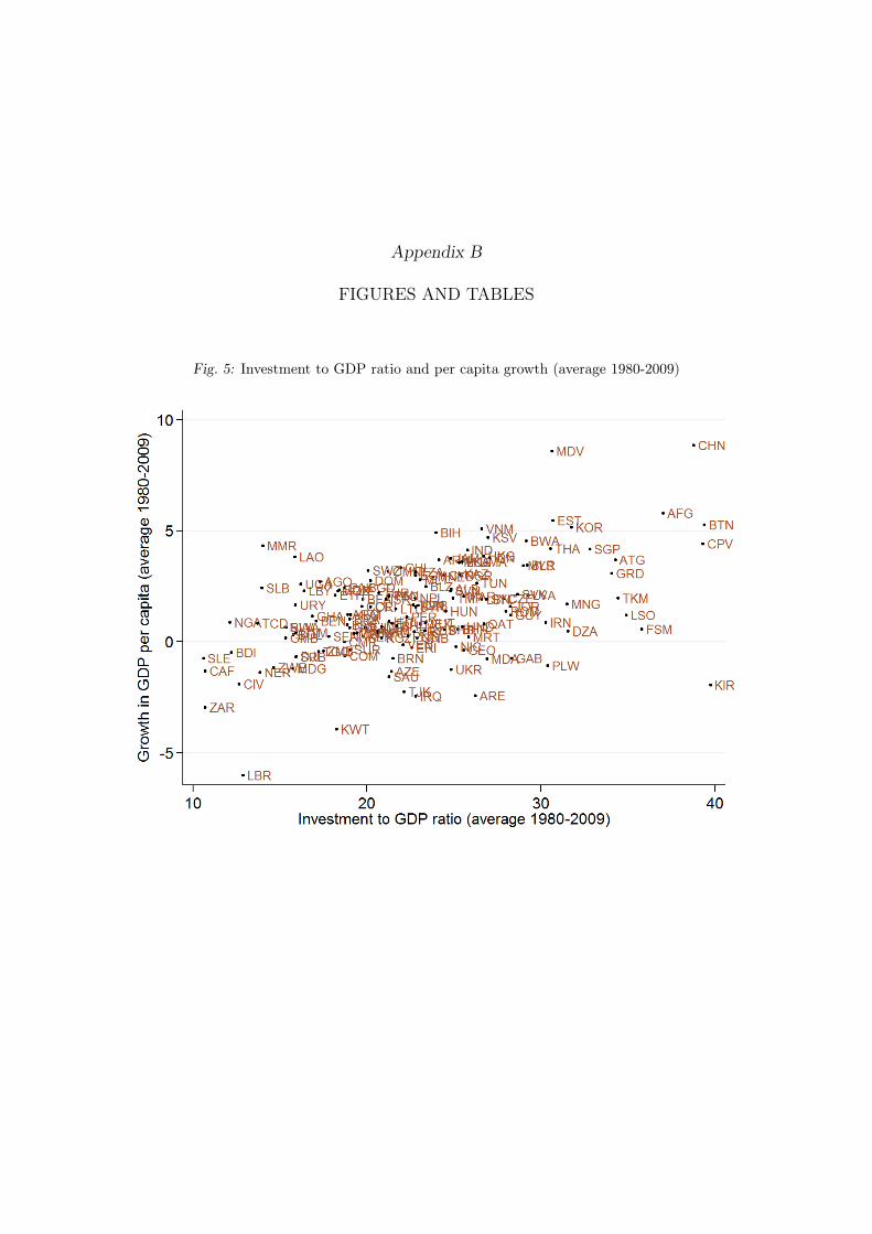
Appendix B

FIGURES AND TABLES

Fig. 5: Investment to GDP ratio and per capita growth (average 1980-2009)

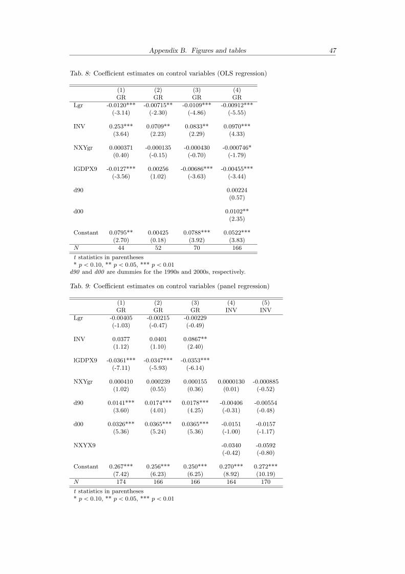
Appendix B. Figures and tables 47

Tab. 8: Coefficient estimates on control variables (OLS regression)

(1) (2) (3) (4)GR GR GR GR

Lgr -0.0120*** -0.00715** -0.0109*** -0.00912***(-3.14) (-2.30) (-4.86) (-5.55)

INV 0.253*** 0.0709** 0.0833** 0.0970***(3.64) (2.23) (2.29) (4.33)

NXYgr 0.000371 -0.000135 -0.000430 -0.000746*(0.40) (-0.15) (-0.70) (-1.79)

lGDPX9 -0.0127*** 0.00256 -0.00686*** -0.00455***(-3.56) (1.02) (-3.63) (-3.44)

d90 0.00224(0.57)

d00 0.0102**(2.35)

Constant 0.0795** 0.00425 0.0788*** 0.0522***(2.70) (0.18) (3.92) (3.83)

N 44 52 70 166t statistics in parentheses* p ă 0.10, ** p ă 0.05, *** p ă 0.01

d90 and d00 are dummies for the 1990s and 2000s, respectively.

Tab. 9: Coefficient estimates on control variables (panel regression)

(1) (2) (3) (4) (5)GR GR GR INV INV

Lgr -0.00405 -0.00215 -0.00229(-1.03) (-0.47) (-0.49)

INV 0.0377 0.0401 0.0867**(1.12) (1.10) (2.40)

lGDPX9 -0.0361*** -0.0347*** -0.0353***(-7.11) (-5.93) (-6.14)

NXYgr 0.000410 0.000239 0.000155 0.0000130 -0.000885(1.02) (0.55) (0.36) (0.01) (-0.52)

d90 0.0141*** 0.0174*** 0.0178*** -0.00406 -0.00554(3.60) (4.01) (4.25) (-0.31) (-0.48)

d00 0.0326*** 0.0365*** 0.0365*** -0.0151 -0.0157(5.36) (5.24) (5.36) (-1.00) (-1.17)

NXYX9 -0.0340 -0.0592(-0.42) (-0.80)

Constant 0.267*** 0.256*** 0.250*** 0.270*** 0.272***(7.42) (6.23) (6.25) (8.92) (10.19)

N 174 166 166 164 170t statistics in parentheses* p ă 0.10, ** p ă 0.05, *** p ă 0.01

Appendix B. Figures and tables 48

Tab. 10: List of countries included in the regressions

Country Code 80s 90s 00s

Argentina ARG 1 1 0Armenia ARM 0 0 1Bahamas BHS 0 1 0Bahrain BHR 1 1 0

Bangladesh BGD 0 0 1Belarus BLR 0 0 1Belize BLZ 0 1 0Benin BEN 0 0 1

Bhutan BTN 0 1 1Bolivia BOL 1 1 1

Botswana BWA 1 1 0Brazil BRA 1 1 1

Bulgaria BGR 0 0 1Burkina Faso BFA 1 0 1

Burundi BDI 0 1 0Cambodia KHM 0 0 1Cameroon CMR 0 1 0

Chile CHL 1 1 1Colombia COL 1 1 1

Congo ZAR 0 0 1Costa Rica CRI 1 1 1

Cote d’Ivoire CIV 0 0 0Croatia HRV 0 0 1Cyprus CYP 1 1 1

Czech Republic CZE 0 0 1Dominican Republic DOM 1 1 1

Ecuador ECU 1 0 0Egypt EGY 1 1 1

El Salvador SLV 0 1 1Estonia EST 0 0 1Ethiopia ETH 1 1 1

Fiji FJI 1 1 0Georgia GEO 0 0 1Ghana GHA 0 0 1

Guatemala GTM 1 1 1Honduras HND 0 0 1

Hong Kong HKG 0 0 1Hungary HUN 0 1 1

India IND 1 1 1Indonesia IDN 1 1 1

Iran IRN 1 1 1Israel ISR 1 1 1

Jamaica JAM 0 1 1Jordan JOR 1 1 1

Kazakhstan KAZ 0 0 1

Country Code 80s 90s 00s

Kenya KEN 1 1 1Korea KOR 1 1 1Latvia LVA 0 0 1

Lesotho LSO 0 1 1Lithuania LTU 0 0 1

Madagascar MDG 0 1 1Malawi MWI 1 0 0

Malaysia MYS 1 1 1Mali MLI 0 0 1

Malta MLT 1 1 1Mauritius MUS 1 1 1

Mexico MEX 1 1 0Mongolia MNG 0 0 1Morocco MAR 1 1 1Namibia NAM 0 0 1

Nepal NPL 1 1 1Nicaragua NIC 1 0 1Pakistan PAK 1 1 1Panama PAN 0 1 0

Papua New Guinea PNG 0 1 0Paraguay PRY 1 1 1

Peru PER 1 1 1Philippines PHL 1 1 1

Poland POL 0 0 1Romania ROM 0 0 1

Russia RUS 0 0 1Seychelles SYC 0 1 1

Sierra Leone SLE 0 0 1Slovak SVK 0 0 1

Slovenia SVN 0 0 1South Africa ZAF 1 1 1

Sri Lanka LKA 1 1 1Syrian Arab Republic SYR 0 1 0

Thailand THA 1 1 1Togo TGO 1 0 0

Trinidad and Tobago TTO 1 0 1Tunisia TUN 0 1 1Turkey TUR 1 1 0Uganda UGA 0 0 1Ukraine UKR 0 0 1Uruguay URY 1 1 1

Venezuela VEN 1 1 0Zambia ZMB 0 0 1

Zimbabwe ZWE 1 0 0Sum 44 52 70

1 indicates that there is available data for that country in the respective decade. Countries withdata available for at least two decades are included in the panel regression. There are 48 countrieswith data available for at least two decades. Toghether they form 126 observations, that are usedto calculate the coefficients. The regression table (Tab. 5 (2)) reports N=166, because "Stata doesnot drop panels with only one observation, because they provide information about the constant,the variance components, the between R-sq, the overall R-sq and the correlation between the uiand Xb" (Drukker, 2002).

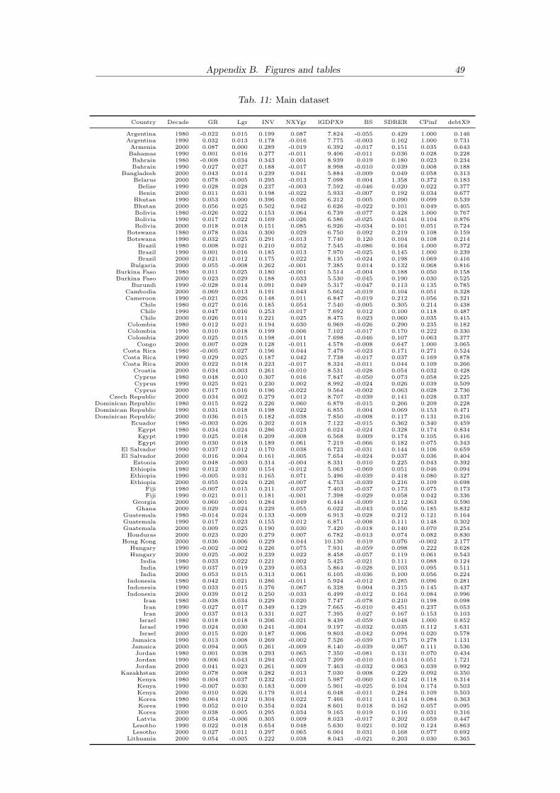
Appendix B. Figures and tables 49

Tab. 11: Main dataset

Country Decade GR Lgr INV NXYgr lGDPX9 BS SDRER CPinf debtX9

Argentina 1980 -0.022 0.015 0.199 0.087 7.824 -0.055 0.429 1.000 0.146Argentina 1990 0.032 0.013 0.178 -0.016 7.775 -0.003 0.162 1.000 0.731Armenia 2000 0.087 0.000 0.289 -0.019 6.392 -0.017 0.151 0.035 0.643Bahamas 1990 0.001 0.016 0.277 -0.011 9.406 -0.011 0.036 0.028 0.228Bahrain 1980 -0.008 0.034 0.343 0.001 8.939 0.019 0.180 0.023 0.234Bahrain 1990 0.027 0.027 0.188 -0.017 8.998 -0.010 0.039 0.008 0.188

Bangladesh 2000 0.043 0.014 0.239 0.041 5.884 -0.009 0.049 0.058 0.313Belarus 2000 0.078 -0.005 0.295 -0.013 7.098 0.004 1.358 0.372 0.183Belize 1990 0.028 0.028 0.237 -0.003 7.592 -0.046 0.020 0.022 0.377Benin 2000 0.011 0.031 0.198 -0.022 5.933 -0.007 0.192 0.034 0.677

Bhutan 1990 0.053 0.000 0.396 0.026 6.212 0.005 0.090 0.099 0.539Bhutan 2000 0.056 0.025 0.502 0.042 6.626 -0.022 0.101 0.049 0.405Bolivia 1980 -0.026 0.022 0.153 0.064 6.739 -0.077 0.428 1.000 0.767Bolivia 1990 0.017 0.022 0.169 -0.026 6.586 -0.025 0.041 0.104 0.876Bolivia 2000 0.018 0.018 0.151 0.085 6.926 -0.034 0.101 0.051 0.724

Botswana 1980 0.078 0.034 0.300 0.029 6.750 0.092 0.219 0.108 0.159Botswana 1990 0.032 0.025 0.291 -0.013 7.740 0.120 0.104 0.108 0.214

Brazil 1980 0.008 0.021 0.210 0.052 7.545 -0.086 0.164 1.000 0.372Brazil 1990 0.001 0.016 0.185 0.013 7.970 -0.025 0.145 1.000 0.239Brazil 2000 0.021 0.012 0.175 0.022 8.135 -0.024 0.198 0.069 0.416

Bulgaria 2000 0.055 -0.008 0.262 -0.001 7.385 0.014 0.132 0.068 0.816Burkina Faso 1980 0.011 0.025 0.180 -0.001 5.514 -0.004 0.188 0.050 0.158Burkina Faso 2000 0.023 0.029 0.188 0.033 5.530 -0.045 0.190 0.030 0.525

Burundi 1990 -0.028 0.014 0.091 0.049 5.317 -0.047 0.113 0.135 0.785Cambodia 2000 0.069 0.013 0.191 0.043 5.662 -0.019 0.104 0.051 0.328Cameroon 1990 -0.021 0.026 0.148 0.011 6.847 -0.019 0.212 0.056 0.321

Chile 1980 0.027 0.016 0.185 0.054 7.540 -0.005 0.305 0.214 0.438Chile 1990 0.047 0.016 0.253 -0.017 7.692 0.012 0.100 0.118 0.487Chile 2000 0.026 0.011 0.221 0.025 8.475 0.023 0.060 0.035 0.415

Colombia 1980 0.012 0.021 0.194 0.030 6.969 -0.026 0.290 0.235 0.182Colombia 1990 0.010 0.018 0.199 0.006 7.102 -0.017 0.170 0.222 0.330Colombia 2000 0.025 0.015 0.198 -0.011 7.698 -0.046 0.107 0.063 0.377

Congo 2000 0.007 0.028 0.128 -0.011 4.578 -0.008 0.647 1.000 3.065Costa Rica 1980 -0.005 0.027 0.196 0.044 7.479 -0.023 0.171 0.271 0.524Costa Rica 1990 0.029 0.025 0.187 0.042 7.738 -0.017 0.037 0.169 0.878Costa Rica 2000 0.022 0.018 0.223 -0.017 8.324 -0.011 0.044 0.109 0.266

Croatia 2000 0.034 -0.003 0.261 -0.010 8.531 -0.028 0.054 0.032 0.428Cyprus 1980 0.048 0.010 0.307 0.016 7.847 -0.050 0.073 0.058 0.225Cyprus 1990 0.025 0.021 0.230 0.002 8.992 -0.024 0.026 0.039 0.509Cyprus 2000 0.017 0.016 0.196 -0.022 9.564 -0.002 0.063 0.028 2.736

Czech Republic 2000 0.034 0.002 0.279 0.012 8.707 -0.039 0.141 0.028 0.337Dominican Republic 1980 0.015 0.022 0.226 0.060 6.879 -0.015 0.266 0.209 0.228Dominican Republic 1990 0.031 0.018 0.198 0.022 6.855 0.004 0.069 0.153 0.471Dominican Republic 2000 0.036 0.015 0.182 -0.038 7.850 -0.008 0.117 0.131 0.216

Ecuador 1980 -0.003 0.026 0.202 0.018 7.122 -0.015 0.362 0.340 0.459Egypt 1980 0.034 0.024 0.286 -0.023 6.024 -0.024 0.328 0.174 0.834Egypt 1990 0.025 0.018 0.209 -0.008 6.568 0.009 0.174 0.105 0.416Egypt 2000 0.030 0.018 0.189 0.061 7.219 -0.066 0.182 0.075 0.343

El Salvador 1990 0.037 0.012 0.170 0.038 6.723 -0.031 0.144 0.106 0.659El Salvador 2000 0.016 0.004 0.161 -0.005 7.654 -0.024 0.037 0.036 0.404

Estonia 2000 0.048 -0.003 0.314 -0.004 8.331 0.010 0.225 0.043 0.392Ethiopia 1980 0.012 0.030 0.154 -0.012 5.063 -0.069 0.051 0.046 0.094Ethiopia 1990 -0.005 0.031 0.165 0.071 5.496 -0.039 0.418 0.080 0.327Ethiopia 2000 0.055 0.024 0.226 -0.007 4.753 -0.039 0.216 0.109 0.698

Fiji 1980 -0.007 0.015 0.211 0.037 7.403 -0.037 0.173 0.075 0.173Fiji 1990 0.021 0.011 0.181 -0.001 7.398 -0.029 0.058 0.042 0.336

Georgia 2000 0.060 -0.001 0.284 0.049 6.444 -0.009 0.112 0.063 0.590Ghana 2000 0.029 0.024 0.229 0.055 6.022 -0.043 0.056 0.185 0.832

Guatemala 1980 -0.014 0.024 0.133 -0.009 6.913 -0.028 0.212 0.121 0.164Guatemala 1990 0.017 0.023 0.155 0.012 6.871 -0.008 0.111 0.148 0.302Guatemala 2000 0.009 0.025 0.190 0.030 7.420 -0.018 0.140 0.070 0.254Honduras 2000 0.023 0.020 0.279 0.007 6.782 -0.013 0.074 0.082 0.830

Hong Kong 2000 0.036 0.006 0.229 0.044 10.130 0.019 0.076 -0.002 2.177Hungary 1990 -0.002 -0.002 0.226 0.075 7.931 -0.059 0.098 0.222 0.628Hungary 2000 0.025 -0.002 0.239 0.022 8.458 -0.057 0.119 0.061 0.543

India 1980 0.033 0.022 0.221 0.002 5.425 -0.021 0.111 0.088 0.124India 1990 0.037 0.019 0.239 0.053 5.864 -0.028 0.103 0.095 0.511India 2000 0.053 0.015 0.313 0.061 6.105 -0.036 0.100 0.056 0.224

Indonesia 1980 0.042 0.021 0.286 -0.011 5.924 -0.012 0.285 0.096 0.281Indonesia 1990 0.033 0.015 0.276 0.067 6.328 0.004 0.315 0.145 0.437Indonesia 2000 0.039 0.012 0.250 -0.033 6.499 -0.012 0.164 0.084 0.996

Iran 1980 -0.038 0.034 0.229 0.020 7.747 -0.078 0.210 0.198 0.098Iran 1990 0.027 0.017 0.349 0.129 7.665 -0.010 0.451 0.237 0.053Iran 2000 0.037 0.013 0.331 0.027 7.395 0.027 0.167 0.153 0.103

Israel 1980 0.018 0.018 0.206 -0.021 8.439 -0.059 0.048 1.000 0.852Israel 1990 0.024 0.030 0.241 -0.004 9.197 -0.032 0.035 0.112 1.631Israel 2000 0.015 0.020 0.187 0.006 9.803 -0.042 0.094 0.020 0.578

Jamaica 1990 0.013 0.008 0.269 -0.002 7.526 -0.039 0.175 0.278 1.131Jamaica 2000 0.094 0.005 0.261 -0.009 8.140 -0.039 0.067 0.111 0.536Jordan 1980 0.001 0.038 0.293 0.065 7.350 -0.081 0.131 0.070 0.434Jordan 1990 0.006 0.043 0.294 -0.023 7.209 -0.010 0.014 0.051 1.721Jordan 2000 0.041 0.023 0.261 0.009 7.463 -0.032 0.063 0.039 0.992

Kazakhstan 2000 0.078 0.008 0.282 0.013 7.030 0.008 0.229 0.092 0.350Kenya 1980 0.004 0.037 0.232 -0.021 5.987 -0.060 0.142 0.118 0.314Kenya 1990 -0.007 0.030 0.183 0.009 5.901 -0.025 0.104 0.174 0.503Kenya 2000 0.010 0.026 0.179 0.014 6.048 -0.011 0.284 0.109 0.503Korea 1980 0.064 0.012 0.304 0.022 7.466 0.011 0.114 0.084 0.363Korea 1990 0.052 0.010 0.354 0.024 8.601 0.018 0.162 0.057 0.095Korea 2000 0.038 0.005 0.295 0.034 9.165 0.019 0.116 0.031 0.316Latvia 2000 0.054 -0.006 0.305 0.009 8.023 -0.017 0.202 0.059 0.447

Lesotho 1990 0.022 0.018 0.654 0.048 5.630 0.021 0.102 0.124 0.863Lesotho 2000 0.027 0.011 0.297 0.065 6.004 0.031 0.168 0.077 0.692

Lithuania 2000 0.054 -0.005 0.222 0.038 8.043 -0.021 0.203 0.030 0.365

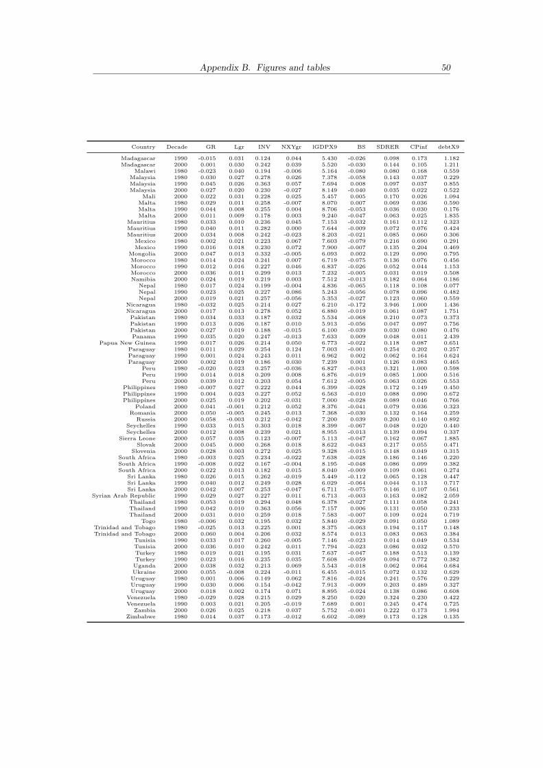
Appendix B. Figures and tables 50

Country Decade GR Lgr INV NXYgr lGDPX9 BS SDRER CPinf debtX9

Madagascar 1990 -0.015 0.031 0.124 0.044 5.430 -0.026 0.098 0.173 1.182Madagascar 2000 0.001 0.030 0.242 0.039 5.520 -0.030 0.144 0.105 1.211

Malawi 1980 -0.023 0.040 0.194 -0.006 5.164 -0.080 0.080 0.168 0.559Malaysia 1980 0.030 0.027 0.278 0.026 7.378 -0.058 0.143 0.037 0.229Malaysia 1990 0.045 0.026 0.363 0.057 7.694 0.008 0.097 0.037 0.855Malaysia 2000 0.027 0.020 0.230 -0.027 8.149 -0.040 0.035 0.022 0.522

Mali 2000 0.022 0.031 0.228 0.025 5.457 0.005 0.170 0.026 1.094Malta 1980 0.029 0.011 0.258 -0.007 8.070 0.007 0.069 0.036 0.590Malta 1990 0.044 0.008 0.255 0.004 8.706 -0.053 0.036 0.030 0.176Malta 2000 0.011 0.009 0.178 0.003 9.240 -0.047 0.063 0.025 1.835

Mauritius 1980 0.033 0.010 0.236 0.045 7.153 -0.032 0.161 0.112 0.323Mauritius 1990 0.040 0.011 0.282 0.000 7.644 -0.009 0.072 0.076 0.424Mauritius 2000 0.034 0.008 0.242 -0.023 8.203 -0.021 0.085 0.060 0.306

Mexico 1980 0.002 0.021 0.223 0.067 7.603 -0.079 0.216 0.690 0.291Mexico 1990 0.016 0.018 0.230 0.072 7.900 -0.007 0.135 0.204 0.469

Mongolia 2000 0.047 0.013 0.332 -0.005 6.093 0.002 0.129 0.090 0.795Morocco 1980 0.014 0.024 0.241 0.007 6.719 -0.075 0.136 0.076 0.456Morocco 1990 0.012 0.016 0.227 0.046 6.837 -0.026 0.052 0.044 1.153Morocco 2000 0.036 0.011 0.299 0.013 7.232 -0.005 0.031 0.019 0.508Namibia 2000 0.024 0.019 0.219 0.003 7.512 -0.013 0.182 0.064 0.186

Nepal 1980 0.017 0.024 0.199 -0.004 4.836 -0.065 0.118 0.108 0.077Nepal 1990 0.023 0.025 0.227 0.086 5.243 -0.056 0.078 0.096 0.482Nepal 2000 0.019 0.021 0.257 -0.056 5.353 -0.027 0.123 0.060 0.559

Nicaragua 1980 -0.032 0.025 0.214 0.027 6.210 -0.172 3.946 1.000 1.436Nicaragua 2000 0.017 0.013 0.278 0.052 6.880 -0.019 0.061 0.087 1.751Pakistan 1980 0.034 0.033 0.187 0.032 5.534 -0.068 0.210 0.073 0.373Pakistan 1990 0.013 0.026 0.187 0.010 5.913 -0.056 0.047 0.097 0.756Pakistan 2000 0.027 0.019 0.188 -0.015 6.100 -0.039 0.030 0.080 0.476Panama 1990 0.035 0.020 0.247 -0.013 7.633 0.009 0.048 0.011 2.439

Papua New Guinea 1990 0.017 0.026 0.214 0.050 6.773 -0.022 0.118 0.087 0.651Paraguay 1980 0.011 0.029 0.254 0.124 7.003 -0.001 0.254 0.202 0.257Paraguay 1990 0.001 0.024 0.243 0.011 6.962 0.002 0.062 0.164 0.624Paraguay 2000 0.002 0.019 0.186 0.030 7.239 0.001 0.126 0.083 0.465

Peru 1980 -0.020 0.023 0.257 -0.036 6.827 -0.043 0.321 1.000 0.598Peru 1990 0.014 0.018 0.209 0.008 6.876 -0.019 0.085 1.000 0.516Peru 2000 0.039 0.012 0.203 0.054 7.612 -0.005 0.063 0.026 0.553

Philippines 1980 -0.007 0.027 0.222 0.044 6.399 -0.028 0.172 0.149 0.450Philippines 1990 0.004 0.023 0.227 0.052 6.563 -0.010 0.088 0.090 0.672Philippines 2000 0.025 0.019 0.202 -0.031 7.000 -0.028 0.089 0.046 0.766

Poland 2000 0.041 -0.001 0.212 0.052 8.376 -0.041 0.079 0.036 0.323Romania 2000 0.050 -0.005 0.245 0.013 7.368 -0.030 0.132 0.164 0.259

Russia 2000 0.058 -0.003 0.212 -0.042 7.200 0.039 0.200 0.140 0.892Seychelles 1990 0.033 0.015 0.303 0.018 8.399 -0.067 0.048 0.020 0.440Seychelles 2000 0.012 0.008 0.239 0.021 8.955 -0.013 0.139 0.094 0.337

Sierra Leone 2000 0.057 0.035 0.123 -0.007 5.113 -0.047 0.162 0.067 1.885Slovak 2000 0.045 0.000 0.268 0.018 8.622 -0.043 0.217 0.055 0.471

Slovenia 2000 0.028 0.003 0.272 0.025 9.328 -0.015 0.148 0.049 0.315South Africa 1980 -0.003 0.025 0.234 -0.022 7.638 -0.028 0.186 0.146 0.220South Africa 1990 -0.008 0.022 0.167 -0.004 8.195 -0.048 0.086 0.099 0.382South Africa 2000 0.022 0.013 0.182 0.015 8.040 -0.009 0.109 0.061 0.274

Sri Lanka 1980 0.026 0.015 0.262 -0.019 5.449 -0.112 0.065 0.128 0.447Sri Lanka 1990 0.040 0.012 0.249 0.028 6.029 -0.064 0.044 0.113 0.717Sri Lanka 2000 0.042 0.007 0.253 -0.047 6.711 -0.075 0.146 0.107 0.561

Syrian Arab Republic 1990 0.029 0.027 0.227 0.011 6.713 -0.003 0.163 0.082 2.059Thailand 1980 0.053 0.019 0.294 0.048 6.378 -0.027 0.111 0.058 0.241Thailand 1990 0.042 0.010 0.363 0.056 7.157 0.006 0.131 0.050 0.233Thailand 2000 0.031 0.010 0.259 0.018 7.583 -0.007 0.109 0.024 0.719

Togo 1980 -0.006 0.032 0.195 0.032 5.840 -0.029 0.091 0.050 1.089Trinidad and Tobago 1980 -0.025 0.013 0.225 0.001 8.375 -0.063 0.194 0.117 0.148Trinidad and Tobago 2000 0.060 0.004 0.206 0.032 8.574 0.013 0.083 0.063 0.384

Tunisia 1990 0.033 0.017 0.260 -0.005 7.146 -0.023 0.014 0.049 0.534Tunisia 2000 0.036 0.010 0.242 0.011 7.794 -0.023 0.086 0.032 0.570Turkey 1980 0.019 0.021 0.195 0.031 7.637 -0.047 0.188 0.513 0.139Turkey 1990 0.023 0.016 0.235 0.035 7.608 -0.059 0.094 0.772 0.382Uganda 2000 0.038 0.032 0.213 0.069 5.543 -0.018 0.062 0.064 0.684Ukraine 2000 0.055 -0.008 0.224 -0.011 6.455 -0.015 0.072 0.132 0.629Uruguay 1980 0.001 0.006 0.149 0.062 7.816 -0.024 0.241 0.576 0.229Uruguay 1990 0.030 0.006 0.154 -0.042 7.913 -0.009 0.203 0.489 0.327Uruguay 2000 0.018 0.002 0.174 0.071 8.895 -0.024 0.138 0.086 0.608

Venezuela 1980 -0.029 0.028 0.215 0.029 8.250 0.020 0.324 0.230 0.422Venezuela 1990 0.003 0.021 0.205 -0.019 7.689 0.001 0.245 0.474 0.725

Zambia 2000 0.026 0.025 0.218 0.037 5.752 -0.001 0.222 0.173 1.994Zimbabwe 1980 0.014 0.037 0.173 -0.012 6.602 -0.089 0.173 0.128 0.135