Embed Size (px)
Citation preview

MACROECONOMICS
B. Schmidt
Hull College of Business
Augusta State University

How I BEGIN Class
• Try to make it REAL and PERSONAL to the student– Discuss current events
• Try to make it FUN– Encourage opinions
• Try to increase COMPREHENSION and RETENTION– Demand participation

FIRST things FIRST:
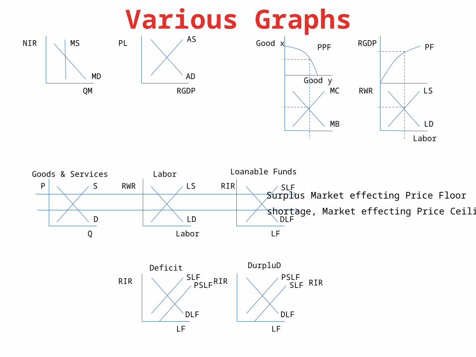
• DETERMINE what they know1. Correctly Draw and Label the following graphs:
S/D, LS/LD, SLF/DLF, AS/AD, MS/MD, PPF, PF

2. What is the immediate short-term result of the following statement

3. And this one…
RIR
DLF
RIR
LF
SLFPSLF
DLF
RIR
LF
PSLFSLF
MC
MB
PPFGood x
Good yLS
LD
PFRGDP
RWR
Labor
MS
MD
NIR
QM
AD
PL
RGDP
AS
S
D
P
Q
LS
LD
RWR
Labor
DLF
RIR
LF
SLFSurplus Market effecting Price Floor
shortage, Market effecting Price Ceiling
Goods & Services Labor Loanable Funds
Deficit DurpluD
Various Graphs

PPF & PF
PPF
Goodx PF
RGDP
GOODy
Labor
Attainable, inefficient Attainable
Unattainable
Unattainable
Attainable, efficient

S
D
S1P
Q
S2
D
S2P
Q
S1
CURVE SHIFTS:$ S = #price of Substitute in production$ S = $price of compliment$ S = $resource price or other input price$ S = #price of the good is expected to rise$ S = $number of sellers$ S = $productivity
D1
D2
SP
Q
D
D2
D1
SP
Q
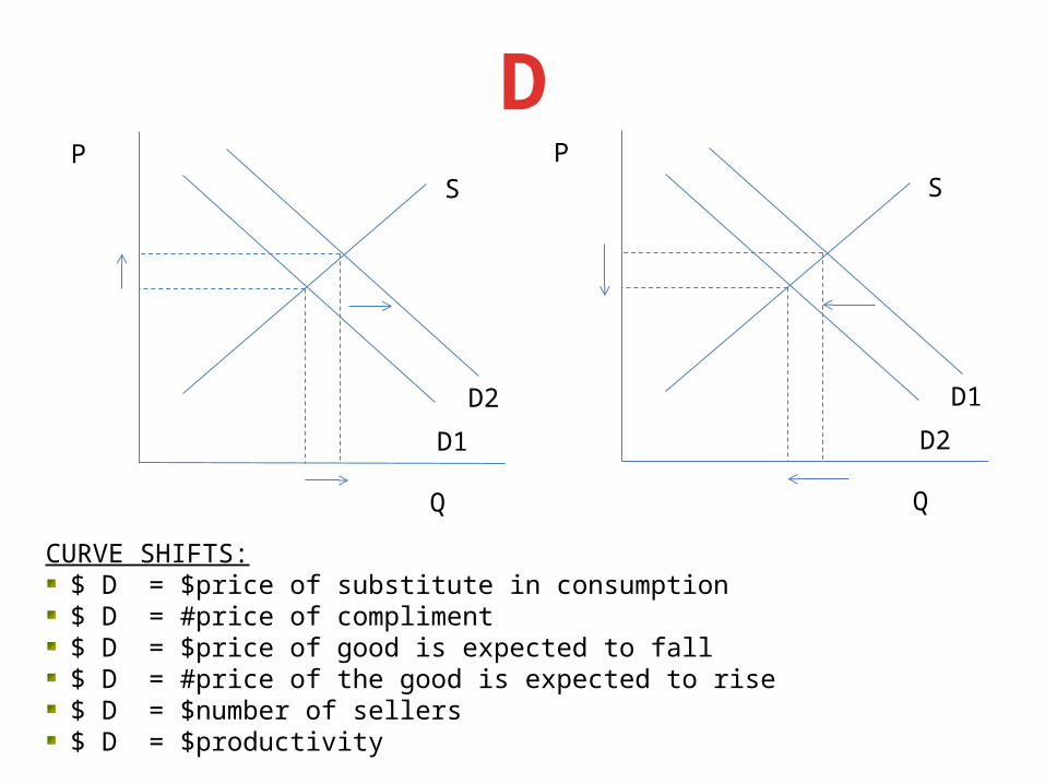
CURVE SHIFTS:$ D = $price of substitute in consumption$ D = #price of compliment$ D = $price of good is expected to fall$ D = #price of the good is expected to rise$ D = $number of sellers$ D = $productivity

LS
LD
LS1WAGE
LABOR
LS2
LD
LS2WAGE
LABOR
LS1
CURVE SHIFTS:$ LS = #taxes $ LS = #unemployment$ LS = $population

LD1
LD2
LSWAGE
LABOR
LD
LD2
LD1
LSWAGE
LABOR
MD
MS2MS1NIR
QM
MD
MS1MS2NIR
QM
MS
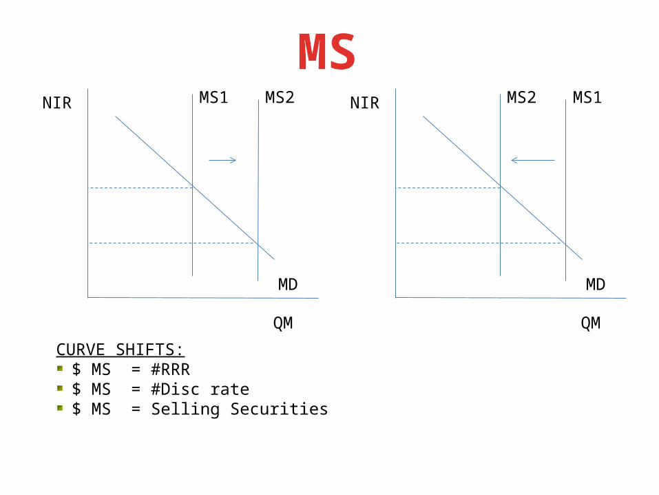
CURVE SHIFTS:$ MS = #RRR$ MS = #Disc rate$ MS = Selling Securities
MD1
MD2
MSNIR
QM
MD2
MD1
MSNIR
QM
MD
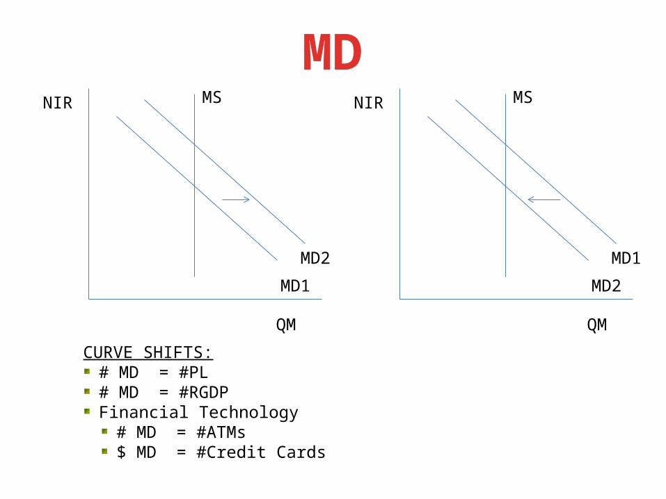
CURVE SHIFTS:# MD = #PL# MD = #RGDPFinancial Technology
# MD = #ATMs$ MD = #Credit Cards
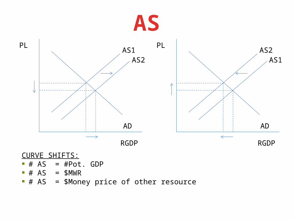
AS
AD
AS1PL
RGDP
AS2
AD
AS2PL
RGDP
AS1
CURVE SHIFTS:# AS = #Pot. GDP# AS = $MWR# AS = $Money price of other resource
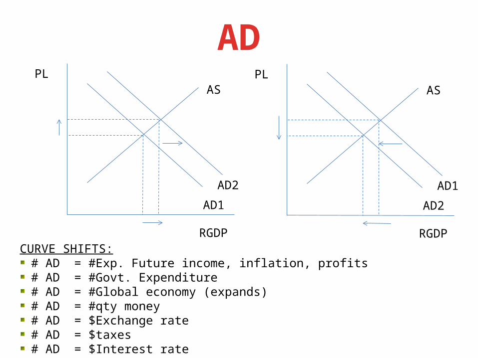
AD
AD1
AD2
ASPL
RGDP
AD2
AD1
ASPL
RGDPCURVE SHIFTS:
# AD = #Exp. Future income, inflation, profits# AD = #Govt. Expenditure# AD = #Global economy (expands)# AD = #qty money# AD = $Exchange rate# AD = $taxes# AD = $Interest rate

SLF
DLF
SLF1RIR
LF
SLF2
DLF
SLF2RIR
LF
SLF1
CURVE SHIFTS:# SLF = #Disp. income# SLF = $Wealth# SLF = $Exp. Future income

DLF
DLF1
DLF2
SLFRIR
LF
DLF2
DLF1
SLFRIR
LF
CURVE SHIFTS:# DLF = #Exp. profit
Bus. Cycle expansionTechnology, successful new products # Population

SURPLUS
LD
LSWAGE
LABOR
D
SP
Q
LABOR SURPLUS SURPLUS
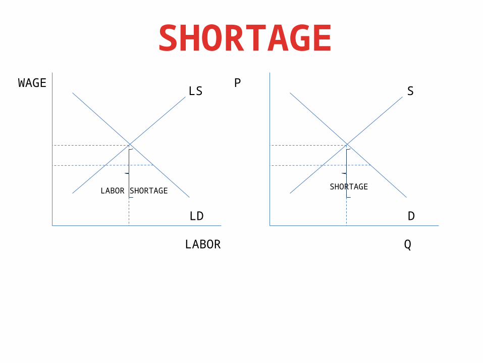
SHORTAGE
LD
LSWAGE
LABOR
D
SP
Q
LABOR SHORTAGE SHORTAGE
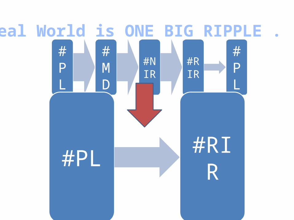
#PL
#MD
#NIR
#RIR
#PL
#PL #RIR
The Real World is ONE BIG RIPPLE . . .
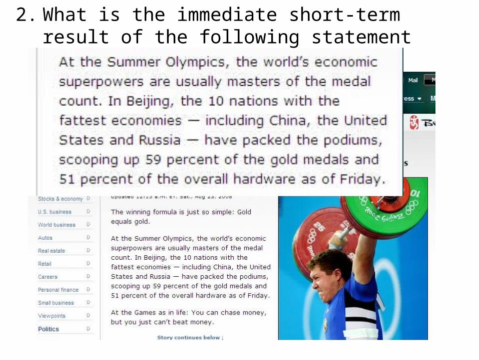
2. What is the immediate short-term result of the following statement

Analyzing the NewsThe article points out that there are anomalies such as Belarus and Jamaica where low GDP countries have won a lot of hardware. In the case of Belarus they also point out that its success could be due to the fact that it was a former Soviet bloc country where the Olympics were a substantial focus.

3. And this one…
Summary: Key Points in the Article
A depression is defined as a severe recession. But what constitutes severe? Since the Great Depression of the 1930s we have had short-lived and relatively shallow downturns in economic activity. But many forecasters and pundits are throwing the term 'depression' around this time. While economic conditions do appear to be dire they are not yet of the same magnitude as the Great Depression.
GDP fell 27 percent between 1929 and 1933. In the current downturn we are only down 2.5 to 3 percent. The stock market lost 90 percent of its value in the Great Depression and we are only down 35 to 40 percent now. One third of all banks failed in the Great Depression. And, while the current bank failures are large, they are numbered in the dozens.
By any metric we are not in a depression. However, the period leading up to the Great Depression has some similarities that are alarming. A period of prosperity in the 1920s led to asset price bubbles and a faltering banking system. However, the current belief is that we learned from our policy mistakes of the 1930s. The Fed has been aggressive in addressing the liquidity crisis. In addition the government appears to be near additional massive fiscal stimulus. Only time will tell whether we have better tools today to keep this downturn classified as a recession.

Analyzing the NewsWhere are we on the business cycle? Unfortunately we won't know until later. Did the aggressive monetary and fiscal stimulus work? I'll let you know in a few years but until then we will all be speculating. Was it enough? Was it too much? Will it get better or worse? It appears we have not been able to prevent downturns nor predict their magnitude. Economic intervention is still more art than science.

PPF

The figure shows the change in the quantity of defense goods and services produced.
Guns Versus Butter
It increases in times of war and decreases in times of peace.

During the 1990s, U.S. production possibilities were shown by PPF0.
President Reagan raised the stakes in the Cold War and the United States was producing at point A.
By mid-1990s, the United States enjoyed a peace dividend and production moved to point B.
Guns Versus Butter
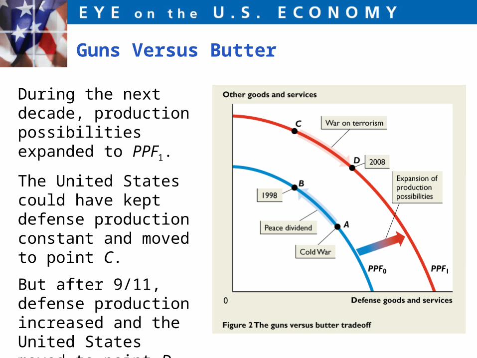
During the next decade, production possibilities expanded to PPF1.
The United States could have kept defense production constant and moved to point C.
But after 9/11, defense production increased and the United States moved to point D.
Guns Versus Butter

Hong Kong’s Rapid Economic Growth
In 1960, Hong Kong’s production possibilities were25 percent of those in the United States.
In 1960, the United States and Hong Kong produced at point A on their respective PPFs.

Hong Kong’s Rapid Economic Growth
Hong Kong allocated more resources to producing capital goods than the United States did.
And by 2008, Hong Kong’s PPF was 80 percent of U.S. PPF.

Hong Kong’s Rapid Economic Growth
If Hong Kong continues to produce at a point like B, allocating more resources to producing capital goods, it will grow more rapidly than the United States.
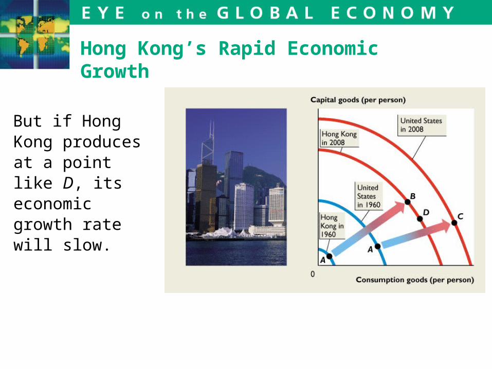
Hong Kong’s Rapid Economic Growth
But if Hong Kong produces at a point like D, its economic growth rate will slow.

What cycle are we currently in?
Business cycle

13.1 BUSINESS-CYCLE DEFINITIONS AND FACTS
U.S. Business-Cycle History
The NBER has identified 33 complete cycles starting from a trough in December 1854.
Over all 33 complete cycles:• The average length of an expansion is 35 months
and the average length of a recession is 18 months.
• The average time from trough to trough is 53 months.
13.1 BUSINESS-CYCLE DEFINITIONS AND FACTS
So over the 152 years since 1854, the U.S. economy has been in:
• Recession for about one third of the time• Expansion for about two thirds of the time.
The 152-year averages hide significant changes that have occurred in the length of a cycle and the relative length of the recession and expansion phases.

13.1 BUSINESS-CYCLE DEFINITIONS AND FACTS
Figure 13.1 summarizes U.S. recession, expansion, and cycle length since 1854.
Recessions have shortened.
Expansions have lengthened, and complete cycles have lengthened.

The National Bureau Calls a Recession
The NBER’s Business Cycle Dating Committee announced in November 2001 that a peak in business activity has occurred in the U.S. economy in March 2001.
To identify the date of the cycle peak, the NBER committee looked at industrial production, employment, real income, and wholesale and retail sales.
The figure on the next slide shows employment.
The National Bureau Calls a Recession
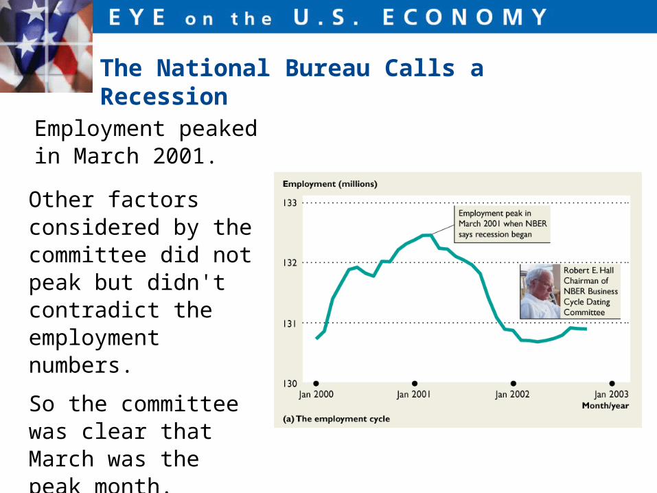
Employment peaked in March 2001.
Other factors considered by the committee did not peak but didn't contradict the employment numbers.
So the committee was clear that March was the peak month.

The NBER committee gives relatively little weight to real GDP.
The National Bureau Calls a Recession
The figure shows that through 2000, real GDP exceeded potential GDP.
Real GDP was shrinking during the first quarter of 2001, before the NBER says the recession began.
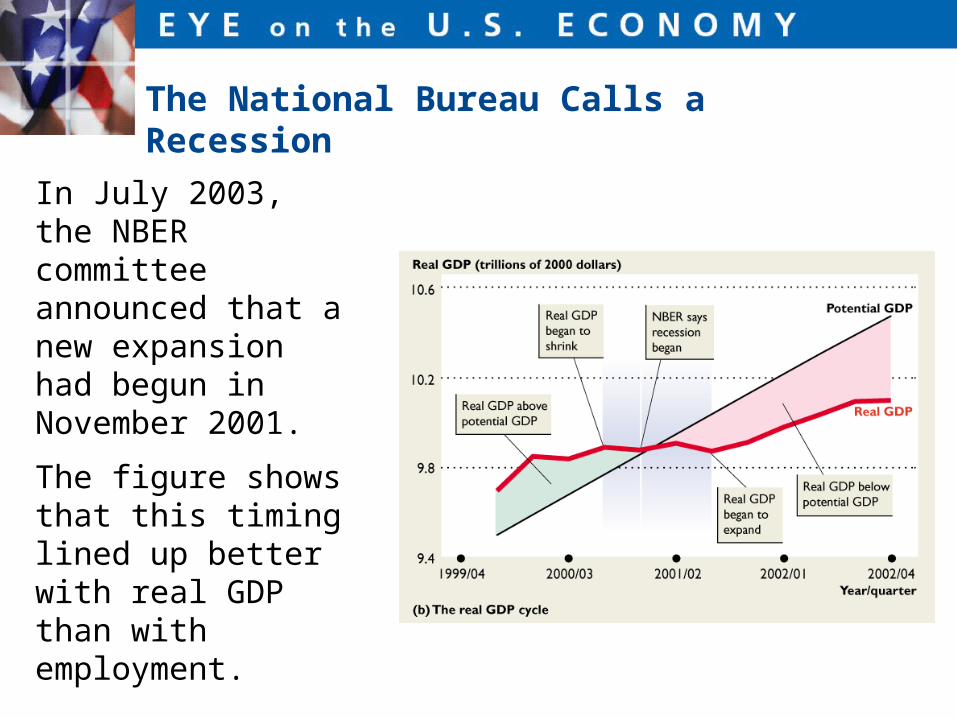
In July 2003, the NBER committee announced that a new expansion had begun in November 2001.
The figure shows that this timing lined up better with real GDP than with employment.
The National Bureau Calls a Recession

The employment trough didn’t occur until April 2002.
The National Bureau Calls a Recession
This lagging of employment behind real GDP is normal and occurs in all expansions.

Every economy has a business cycle, but they differ in severity and timing.
The Global Business Cycle
The U.S. cycle in the early 1908s was the most severe.
The U.S. cycle leads the cycle in Europe and Japan.
Japan’s cycle has taken a downward trend since early 1990s.

The figure shows the business cycle in the world economy.
The Global Business Cycle
The figure shows no recession in the world as a whole since 1980.
and that the Asian economies are driving the world economy.

In September 1973, OPEC cut production and raised the price of crude oil to $10 a barrel—$30 in 2000 dollars.
Oil Price Cycles in the U.S. and Global Economies
In United States, Europe, Japan and developed nations went into recession.
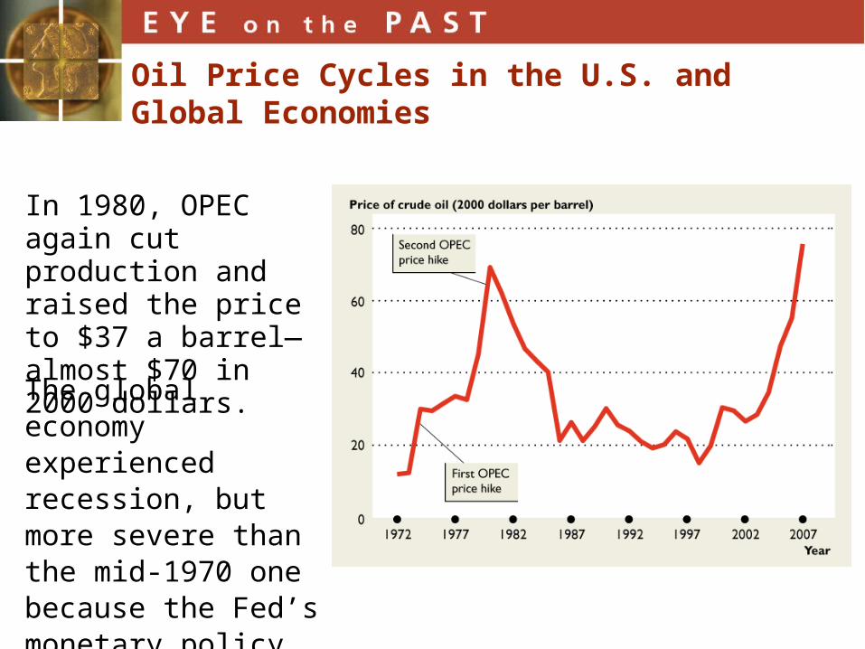
In 1980, OPEC again cut production and raised the price to $37 a barrel—almost $70 in 2000 dollars.
Oil Price Cycles in the U.S. and Global Economies
The global economy experienced recession, but more severe than the mid-1970 one because the Fed’s monetary policy cut aggregate demand.
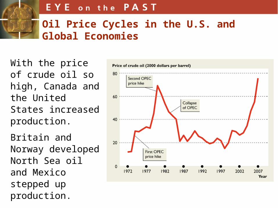
With the price of crude oil so high, Canada and the United States increased production.
Britain and Norway developed North Sea oil and Mexico stepped up production.
The price tumbled.
Oil Price Cycles in the U.S. and Global Economies

Strong Asian demand for oil increased its price in the 2000s.
By 2007, the price has surged to almost $60 a barrel.
By the summer of 2008, the price was $145 a barrel.
Oil Price Cycles in the U.S. and Global Economies

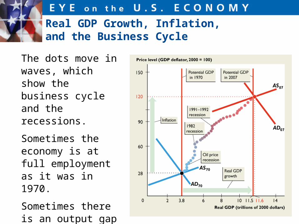
Each dot represents a year between 1970 and 2007.
Dots move rightward, which shows economic growth.
Dots move upward, which shows inflation.
Real GDP Growth, Inflation, and the Business Cycle
Real GDP Growth, Inflation, and the Business Cycle
The dots move in waves, which show the business cycle and the recessions.
Sometimes the economy is at full employment as it was in 1970.
Sometimes there is an output gap as in 2007.

GDP /
HDI

MEASURING U.S. GDP
The relationship between GDP, GNP, and disposable personal income.

THE USE AND LIMITATIONS OF REAL GDP
The shaded periods show the recessions—periods of falling production that lasts for at least six months.

Making Sense of the Numbers
To use the GDP numbers in a news report, you must first check whether the reporter is referring to nominal GDP or real GDP.
Using U.S. real GDP per person, check how your income compares with the average income in the United States.
When you see GDP numbers for other countries, compare your income with that of a person in France, or Canada, or China.
Making GDP Personal
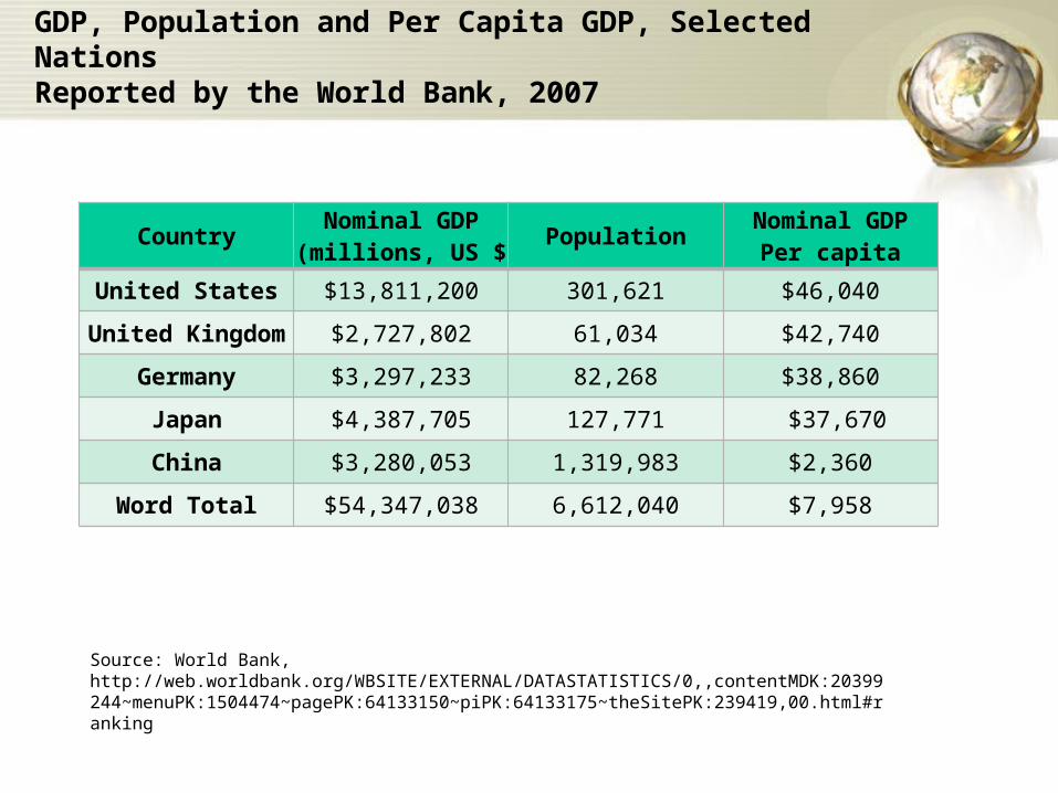
GDP, Population and Per Capita GDP, Selected NationsReported by the World Bank, 2007
Country Nominal GDP(millions, US $ Population Nominal GDP
Per capita
United States $13,811,200 301,621 $46,040
United Kingdom $2,727,802 61,034 $42,740
Germany $3,297,233 82,268 $38,860
Japan $4,387,705 127,771 $37,670
China $3,280,053 1,319,983 $2,360
Word Total $54,347,038 6,612,040 $7,958
Source: World Bank,http://web.worldbank.org/WBSITE/EXTERNAL/DATASTATISTICS/0,,contentMDK:20399244~menuPK:1504474~pagePK:64133150~piPK:64133175~theSitePK:239419,00.html#ranking

U.S. GDP Second Quarter 2008(Current Dollars, Annual Rate)
+C (Consumption) $10,138.5 (billions)
+I (Investment) $2,000.9
+G (Government) $2,873.7
+X (Exports) $1,923.2
-M (Imports) $2,641.4
(Net) (-718.2)
= GDP $14,294.5*
Source: BEA, www.bea.gov/national.nipaweb/TableView.asp?SelectedTable=5&Freq=Qtr&FirstYear=2006&LastYear=2008

The Human Development Index
The figure shows the relationship between real GDP per person and the Human Development Index (HDI).
Each dot represents a country.
The small Africa country of Sierra Leone has the lowest HDI and the second lowest real GDP per person.
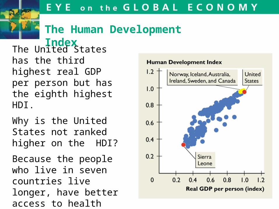
The Human Development Index
The United States has the third highest real GDP per person but has the eighth highest HDI.
Why is the United States not ranked higher on the HDI?
Because the people who live in seven countries live longer, have better access to health care and education than do Americans.

How Fast Has Real GDP per Person Grown?
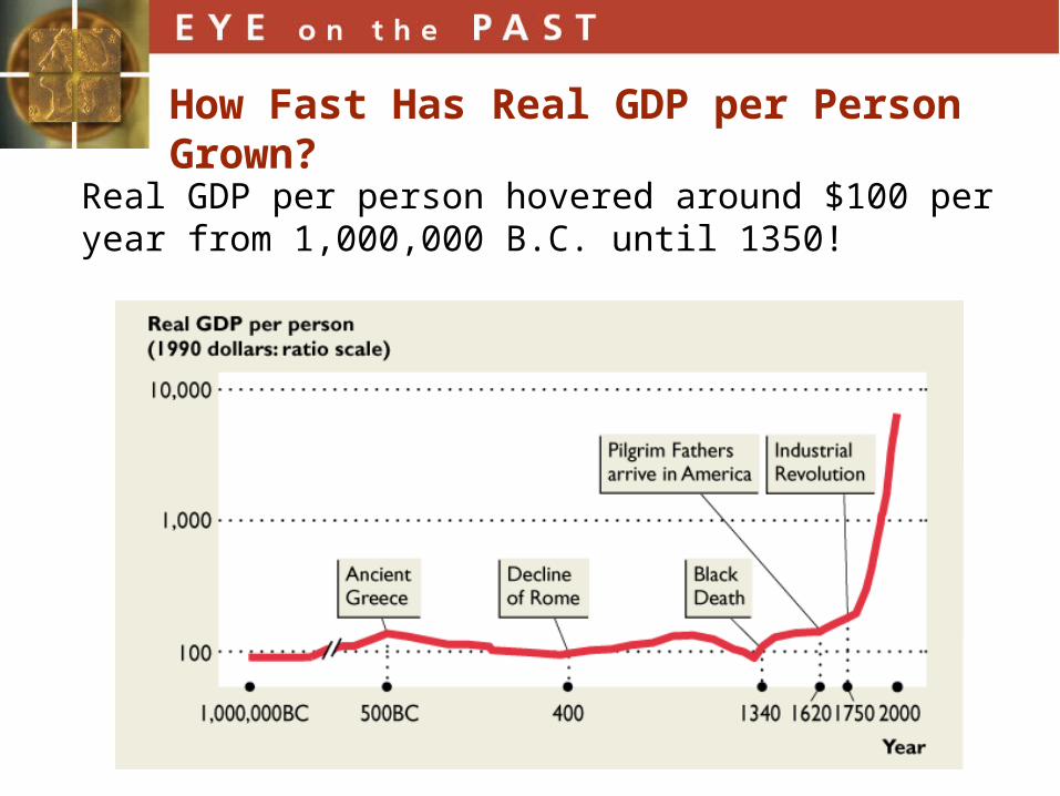
This figure shows the estimates of 1 million years of real GDP per person (in 2000 U.S. dollars) .
How Fast Has Real GDP per Person Grown?
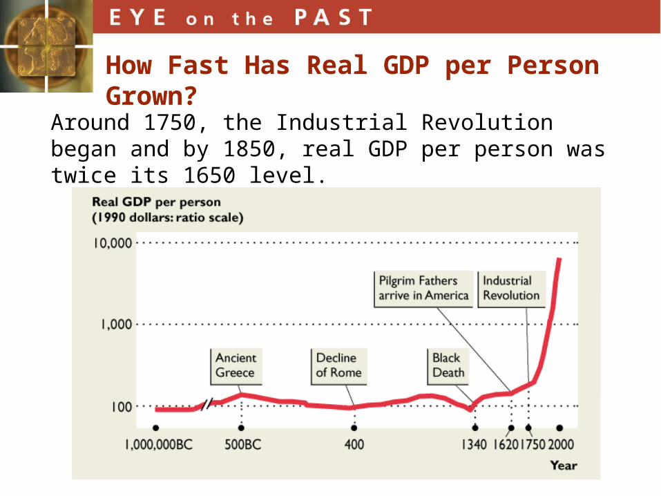
Real GDP per person hovered around $100 per year from 1,000,000 B.C. until 1350!
How Fast Has Real GDP per Person Grown?
Around 1750, the Industrial Revolution began and by 1850, real GDP per person was twice its 1650 level.

How Fast Has Real GDP per Person Grown?
By 1950, real GDP per person was more than five times its 1850 level. And by 2000, it was four times its 1950 level.
How Fast Has Real GDP per Person Grown?
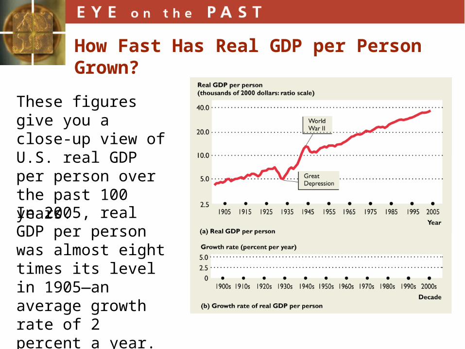
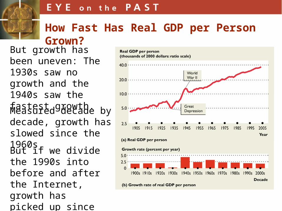
These figures give you a close-up view of U.S. real GDP per person over the past 100 years.
In 2005, real GDP per person was almost eight times its level in 1905—an average growth rate of 2 percent a year.
How Fast Has Real GDP per Person Grown?
But growth has been uneven: The 1930s saw no growth and the 1940s saw the fastest growth.
Measured decade by decade, growth has slowed since the 1960s.
But if we divide the 1990s into before and after the Internet, growth has picked up since 1994.

9.2 THE SOURCES OF ECONOMIC GROWTH
Labor productivity growth depends on• Physical capital growth• Human capital growth• Technological advances
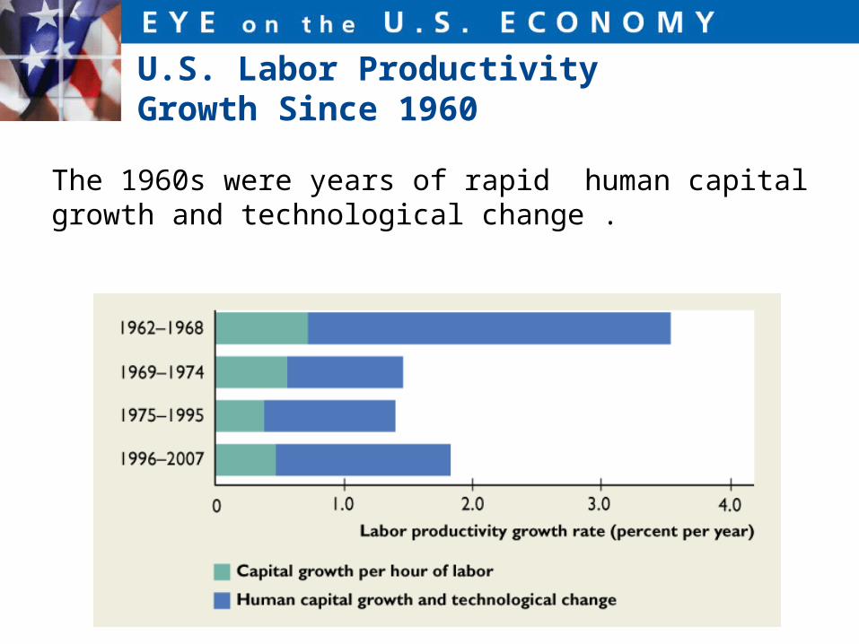
U.S. Labor Productivity Growth Since 1960
The 1960s were years of rapid human capital growth and technological change .
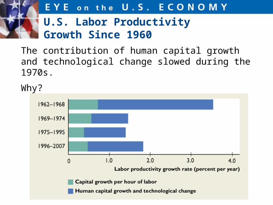
U.S. Labor Productivity Growth Since 1960
The contribution of human capital growth and technological change slowed during the 1970s.
Why?
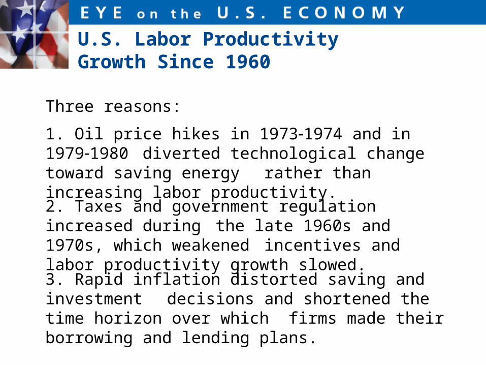
U.S. Labor Productivity Growth Since 1960
Three reasons:
1. Oil price hikes in 19731974 and in 19791980 diverted technological change toward saving energy rather than increasing labor productivity.
2. Taxes and government regulation increased during the late 1960s and 1970s, which weakened incentives and labor productivity growth slowed.
3. Rapid inflation distorted saving and investment decisions and shortened the time horizon over which firms made their borrowing and lending plans.
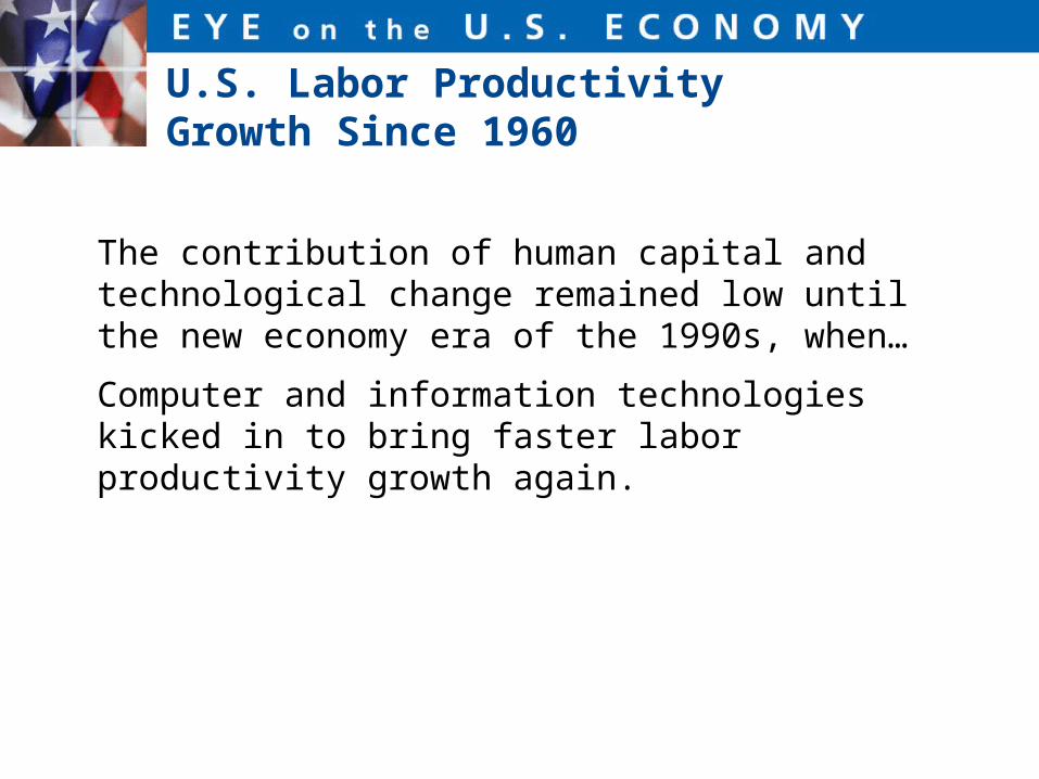
U.S. Labor Productivity Growth Since 1960
The contribution of human capital and technological change remained low until the new economy era of the 1990s, when…
Computer and information technologies kicked in to bring faster labor productivity growth again.

How You Influence and Are Influenced by Economic Growth
Many of the choices that you make affect your personal economic growth rate—the pace of expansion of your own standard of living.
These same choices, in combination with similar choices made by millions of other people, have a profound effect on the economic growth of the nation and the world.
The most important of these choices right now is your choice to increase your human capital.

How You Influence and Are Influenced by Economic Growth
A choice that will become increasingly important later in your life is to accumulate a pension fund.
This choice provides a source of income for you when you eventually retire.
But it also provides financial resources that firms can use to finance the expansion of physical capital.
Not only do your choices influence economic growth; economic growth also has a big influence on you—on how you earn your income and on the standard of living that your income makes possible.

How You Influence and Are Influenced by Economic Growth
Because of economic growth, the jobs available today are more interesting and less dangerous and strenuous than those of 100 years ago.
And today’s jobs are hugely better paid.
But for many of us, economic growth means that we must accept change and be ready to learn new skills and get new jobs.

H u m a n C a p i t a l
J o b s d e s t r o y e d / c r e a t e d

Over the past 65 years, the number of people who work on farms and who produce goods have decreased.
Changes in What We Produce
While the number of people who produce services has expanded.

Over the past 90 years, the amount of education people receive has increased.
Changes in Human Captical
The importance of education has become known and more people are making sacrifices to achieve educational goals

Changes in How We Produce in the New Economy
The new economy consists of the jobs and businesses that produce and use computers and equipment powered by computer chips.
In each pair of photos, the new technology enables capital to replace labor.

Changes in How We Produce in the New Economy
In the top pair of images, illustrates how the ATM (capital) is replacing many bank tellers (labor).
In the bottom pair of images illustrates how a flight check-in machine (capital) is replacing many check-in clerks (labor).

Changes in How We Produce in the New Economy
The number of bank teller and airline check-in clerk jobs is shrinking.
But new technologies are creating a range of new jobs for people who make, program, install, and repair these new machines.
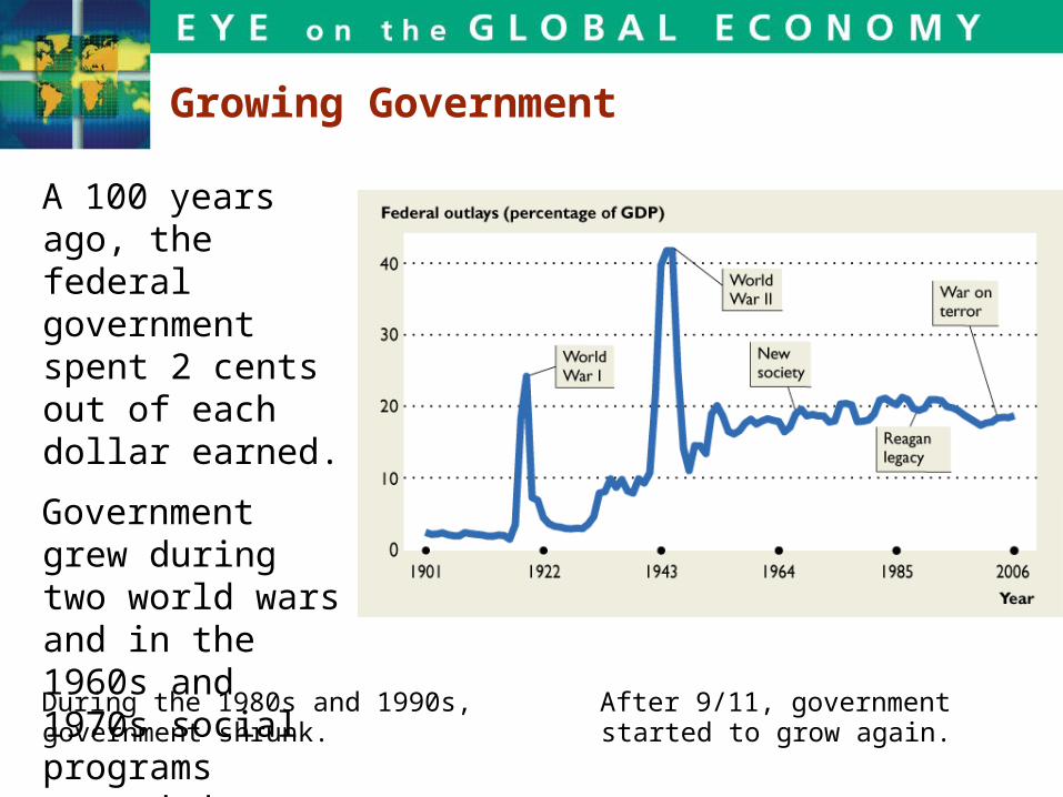
A 100 years ago, the federal government spent 2 cents out of each dollar earned.
Government grew during two world wars and in the 1960s and 1970s social programs expanded.
After 9/11, government started to grow again.
During the 1980s and 1990s, government shrunk.
Growing Government

How can you use the facts and trends about what, how, and for whom goods and services are produced in the U.S. and global economies?
As you think about your future career, you know that a job in manufacturing is likely to be tough. A job in services is more likely to lead to success.
What sort of job will you take?
As you think about the stand you will take on the political question of protecting U.S. jobs, you are better informed.
But how will you vote?
The U.S. and Global Economies in Your Life

u n e m p l o y m e n t
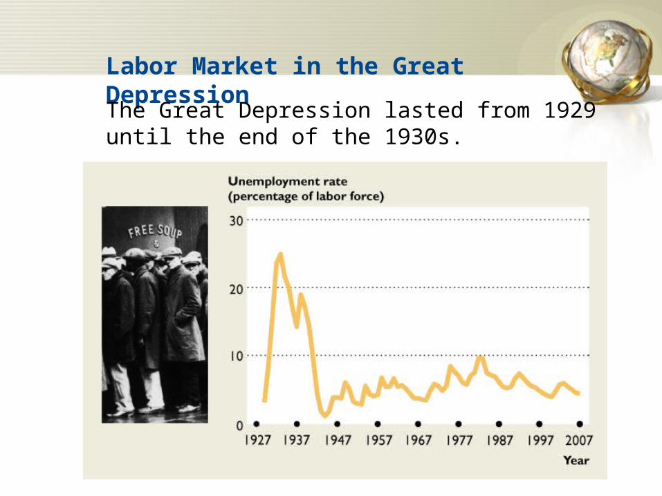
Labor Market in the Great Depression
The Great Depression lasted from 1929 until the end of the 1930s.
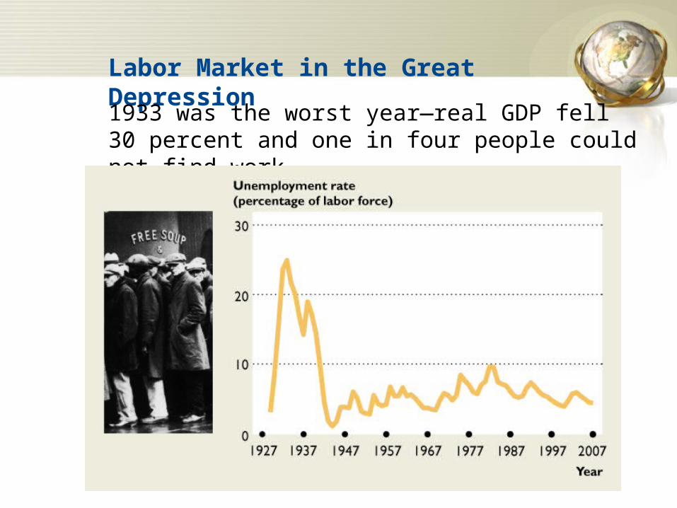
Labor Market in the Great Depression
1933 was the worst year—real GDP fell 30 percent and one in four people could not find work.

7.1 LABOR MARKET INDICATORS
Figure 7.1 shows population labor force categories.
The figure shows the data for August 2007.

7.2 LABOR TRENDS AND FLUCTUATIONS
The unemployment rate increases in recessions and decreases in expansions.

7.2 LABOR TRENDS AND FLUCTUATIONS
The labor force participation rate of men has decreased.
The average participation rate of both sexes hasincreased.
7.2 LABOR TRENDS AND FLUCTUATIONS
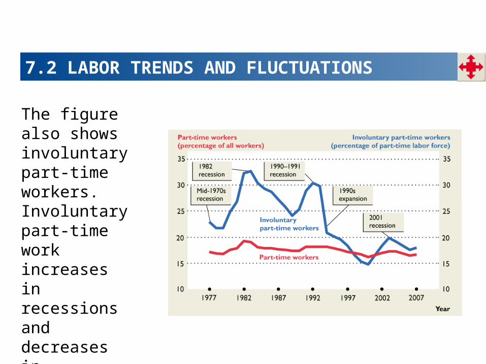
The figure also shows involuntary part-time workers.
Involuntary part-time work increases in recessions and decreases in expansions.

7.3 SOURCES AND TYPES OF UNEMPLOYMENT
Figure 7.6 shows unemployment by reasons.
Job leavers are the smallest group, and their number fluctuates little.
Job losers are the biggest group, and their number fluctuates most.

7.3 SOURCES AND TYPES OF UNEMPLOYMENT
Duration and Demographics of Unemployment
On the average from 1997 to 2007, blacks experienced more than twice the unemployment rate of whites.

Figure 7.8(a)shows the U.S. unemployment rate from 1977 to 2007.
As the unemployment rate fluctuates around the natural rate unemployment, …
7.3 SOURCES AND TYPES OF UNEMPLOYMENT
Cyclical unemployment is negative (shaded red) and positive (shaded blue).

Figure 7.8 shows the relationship between unemployment and real GDP.
As the unemployment rate fluctuates around the natural rate unemployment in part (a), real GDP fluctuates around potential GDP in part (b).
7.3 SOURCES AND TYPES OF UNEMPLOYMENT

Unemployment Around the World
The U.S. unemployment rate lies in the middle of the range experienced by other countries.

Unemployment Around the World
Canada, the United Kingdom, and the Eurozone have higher unemployment rates than the United States and Japan.
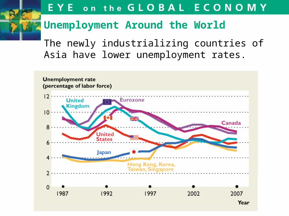
Unemployment Around the World
The newly industrializing countries of Asia have lower unemployment rates.

Unemployment Around the World
The differences in unemployment rate were much greater during the 1980s and 1990s than in the 2000s.
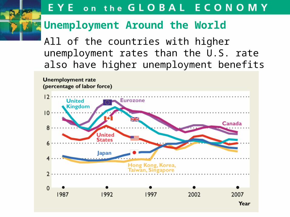
Unemployment Around the World
All of the countries with higher unemployment rates than the U.S. rate also have higher unemployment benefits and more regulated labor markets.

Before 1980, unemploy-ment rates in the United States and Canada were similar.
Unemployment Benefits and theNatural Unemployment Rate

The key change in the 1980s was an increase in Canadian unemploy-ment benefits.
Unemployment Benefits and theNatural Unemployment Rate

Unemployment Benefits and theNatural Unemployment Rate
Almost 100 percent of Canada’s unemployed people receive benefits compared to 38 percent in the United States.
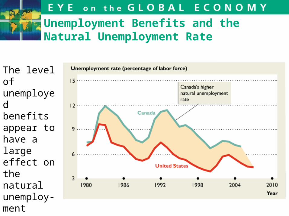
Unemployment Benefits and theNatural Unemployment Rate
The level of unemployed benefits appear to have a large effect on the natural unemploy-ment rate.

Women in the Labor Force
The labor force participation rates of women in most advanced countries has increased since the 1960s, but the level of participation varies a great deal.

Women in the Labor Force
Cultural factors play a role in determining national differences in women’s choices, but economic factors such as education will ultimate dominate cultural ones.
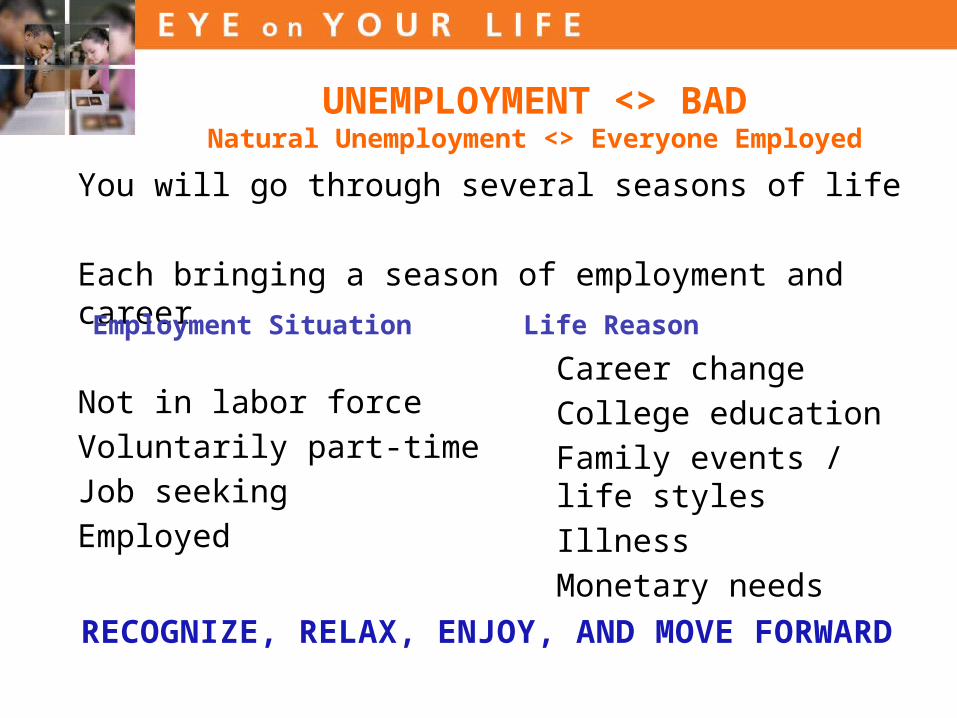
You will go through several seasons of life
Each bringing a season of employment and career
Not in labor force
Voluntarily part-time
Job seeking
Employed
UNEMPLOYMENT <> BADNatural Unemployment <> Everyone Employed
Career change
College education
Family events / life styles
Illness
Monetary needs
Employment Situation Life Reason
RECOGNIZE, RELAX, ENJOY, AND MOVE FORWARD

WHY ARE YOU HERE
PLU’s
Stipend
Have to do something
Inspiration
Collaboration
Encouragement


INSPIRE
ENCOURAGE
EXPECT

G o v t s p e n d i n g

What We Produce

Income Distribution

Federal Government
Revenue
Expenditures
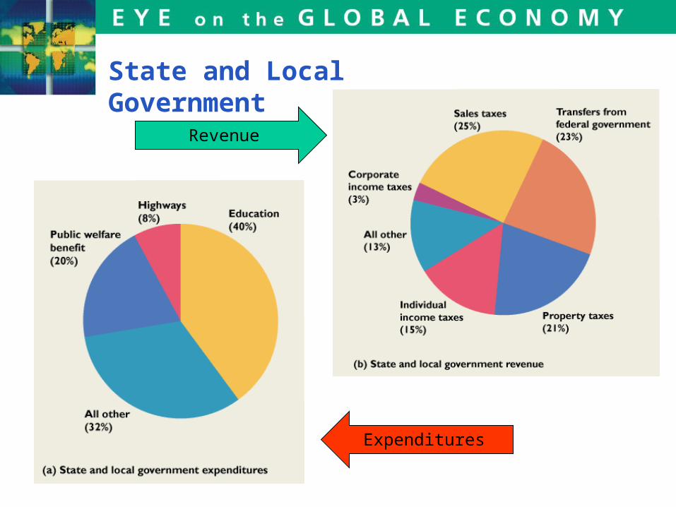
State and Local Government
Revenue
Expenditures
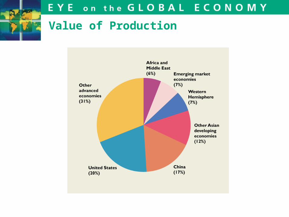
Value of Production

CoalNatural
GasOIL
Energy Sources
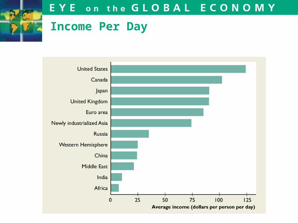
Income Per Day

I n fl a t i o n ,
N W R / R W R ,
C P I

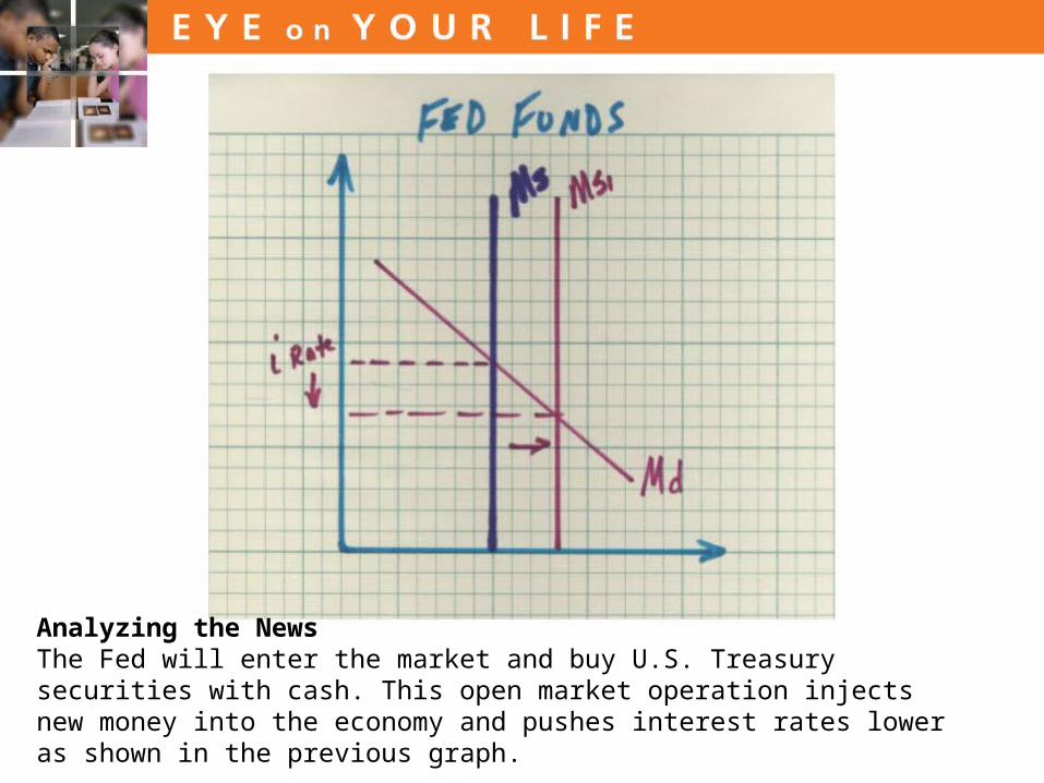
Analyzing the NewsThe Fed will enter the market and buy U.S. Treasury securities with cash. This open market operation injects new money into the economy and pushes interest rates lower as shown in the previous graph.

These data show that inflation became a persistent problem only after 1900.
During the preceding 600 years, inflation was almost unknown.
700 Years of Inflation and Deflation
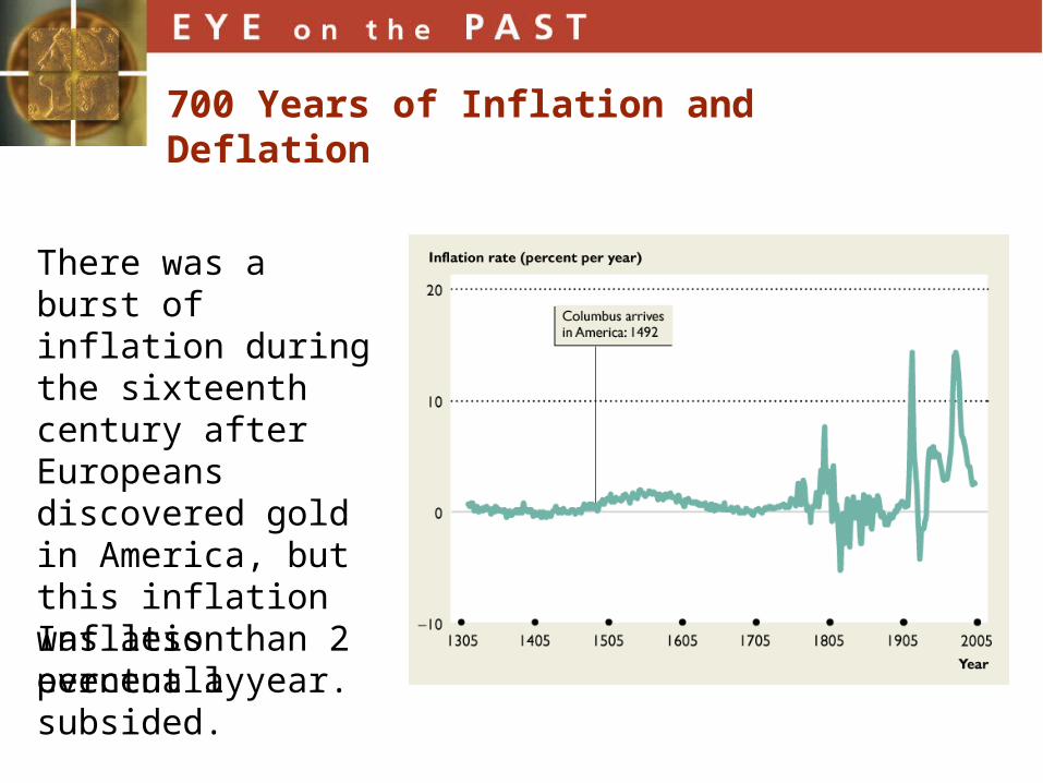
There was a burst of inflation during the sixteenth century after Europeans discovered gold in America, but this inflation was less than 2 percent a year.
Inflation eventually subsided.
700 Years of Inflation and Deflation

The Industrial Revolution was a temporary burst of inflation.
The graph provides dramatic evidence that inflation took off during the last century.
700 Years of Inflation and Deflation

The figure shows the cost of a first-class letter since 1907.
The green line is the nominal price—the actual price of a stamp in the dollars (cents) of the year in question.
The Nominal and Real Price of a First-Class Letter

The red line is the real price—the price in terms ofthe 2007 dollar.
The nominal price has gradually increased, but the real price has fluctuated—sometimes rising and sometimes falling.
The Nominal and Real Price of a First-Class Letter

The highest real price, 45 cents, occurred in 1933 and the lowest real price, 19 cents, occurred in 1920.
The Nominal and Real Price of a First-Class Letter
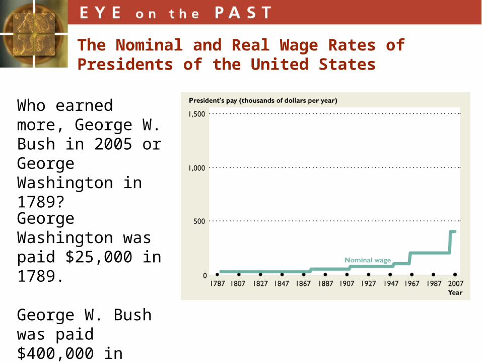
Who earned more, George W. Bush in 2005 or George Washington in 1789?
George Washington was paid $25,000 in 1789.
George W. Bush was paid $400,000 in 2005.
The Nominal and Real Wage Rates of Presidents of the United States

The real wage rate (the red line) has followed a remarkable course.
Expressed in 2005 dollars, George Washington earned $251,000 a year—more than George W. Bush’s $400,000.
The Nominal and Real Wage Rates of Presidents of the United States
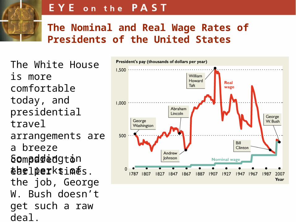
The White House is more comfortable today, and presidential travel arrangements are a breeze compared to earlier times.
So adding in the perks of the job, George W. Bush doesn’t get such a raw deal.
The Nominal and Real Wage Rates of Presidents of the United States

6.3 NOMINAL AND REAL VALUES
Figure 6.4 shows nominal and real wage rates: 1982–2006.
The nominal wage rate has increased every year since 1982.
The real wage rate decreased slightly from 1982 through the mid-1990s, after which increased slightly.

Suppose you have a student loan of $80,000.
Suppose that the CPI rises by 3 percent a year each year from now (2008) through 2028.
Also suppose that the nominal interest rate on your loan is fixed at 5 percent a year.
How much will a $100 repayment cost you in 2008 dollars, when you start to pay off your loan in 2018?
How much will a $100 repayment cost you in 2008 dollars, when you make your final payment in 2028?
What is the real interest rate that you will have paid?
Using the CPI
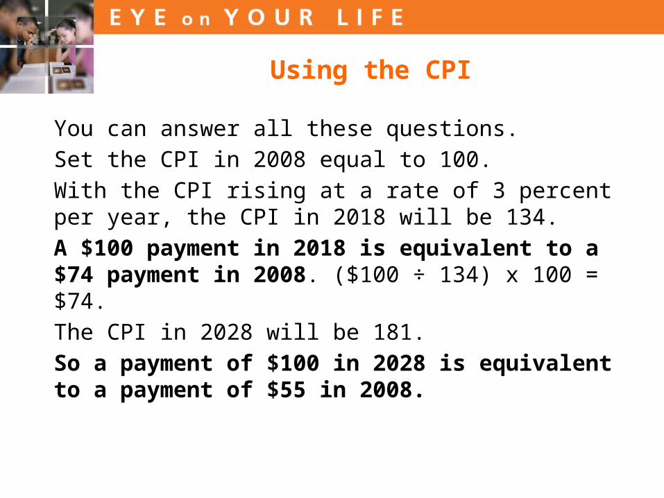
You can answer all these questions.
Set the CPI in 2008 equal to 100.
With the CPI rising at a rate of 3 percent per year, the CPI in 2018 will be 134.
A $100 payment in 2018 is equivalent to a $74 payment in 2008. ($100 ÷ 134) x 100 = $74.
The CPI in 2028 will be 181.
So a payment of $100 in 2028 is equivalent to a payment of $55 in 2008.
Using the CPI

The further in the future a payment is made, the less is your $100 payment in today’s dollars.
Your real interest rate is the 5 percent a year nominal interest rate minus the 3 percent a year inflation rate.
Your real interest rate is 2 percent per year.
Using the CPI

i n v e s t m e n t ,
S a v i n g ,
R i r
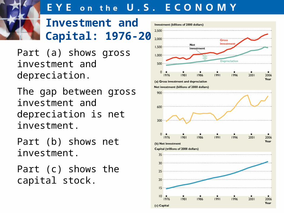
Investment andCapital: 1976-2006
Part (a) shows gross investment and depreciation.
The gap between gross investment and depreciation is net investment.
Part (b) shows net investment.
Part (c) shows the capital stock.

Investment andCapital: 1976-2006
Gross investment increases in most years and increased rapidly during the booming 1990s, but it decreases in recession years—see part (a) of the figure.
Recession years are highlighted in red.

Investment andCapital: 1976-2006
Depreciation increases in most years.
Like gross investment, net investment increased rapidly during the 1990s expansion.
Because net investment is always positive, the quantity of capital increases each year despite huge swings in net investment because the quantity of capital is large in comparison to net investment.
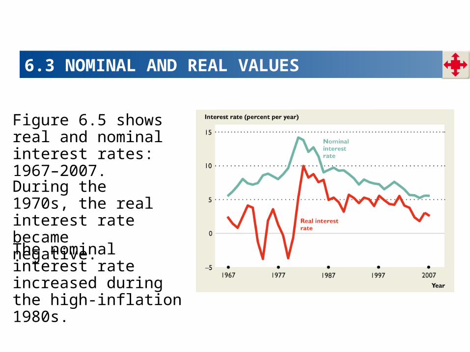
6.3 NOMINAL AND REAL VALUES
Figure 6.5 shows real and nominal interest rates: 1967–2007.
The nominal interest rate increased during the high-inflation 1980s.
During the 1970s, the real interest rate became negative.

The real interest rate paid by big corporations fell from 5.5 percent a year in 2001 to 2.5 percent a year in 2005.
Alan Greenspan said he was puzzled that the real interest rate was falling when the U.S. government budget deficit was growing.
Why did the real interest rate fall?
The answer lies in the global loanable funds market.
Interest Rate Puzzle

Global saving increased and the supply of loanable funds increased from SLF01 in 2001 to SLF05 in 2005.
U.S. saving decreased and U.S. borrowing from the rest of the world increased strongly during these years.
The Chinese, Japanese, and Germans all have much higher saving rates than do Americans.
Interest Rate Puzzle

Think about the amount of saving that you do.
How much of your disposable income do you save? Is it a positive amount or a negative amount?
If you save a positive amount, what do you do with your savings?
•Do you put them in a bank, in the stock market, in bonds, or just keep money at home?
What is the interest rate you earn on your savings?
Your Saving, Investment, and Loanable Funds Market

If you save a negative amount, just what does that mean?
It means that you have a deficit (like a government deficit). You’re spending more than your disposable income.
•In this case, how do you finance your deficit? Do you get a student loan? Do you run up an outstanding credit card balance?
How much do you pay to finance your negative saving (your dissaving)?
How do you think your saving will change when you graduate and get a better-paying job?
• CURVE SHIFTS:# SLF = #Disp. income# SLF = $Wealth# SLF = $Exp. Future income
Your Saving, Investment, and Loanable Funds Market

Also think about the amount of investment that you do.
You are investing in your human capital by being in school. What is this investment costing you? How are you financing this investment?
When you graduate, you will need to decide whether to invest in an apartment or a house or to rent your home.
How would you make a decision whether to buy or rent a home?
Would it be smart to borrow $300,000 to finance the purchase of a home? How would the interest rate influence your decision?
Your Saving, Investment, and Loanable Funds Market

B a n k s ,M o n e y A b r o a d ,
C r e d i t C a r d s ,F e d w a t c h i n g ,
H y p e r i n fl a t i o n

11.3 THE FEDERAL RESERVE SYSTEM
Figure 11.4 shows the 12 Federal Reserve districts.
Each FederalReserve district has its ownFederal Reserve Bank.
The Board of Governors of the Federal Reserve System islocated in Washington, D.C.

Figure 11.2 shows the institutions of the banking system.
The Federal Reserve regulates and influences the activities of the commercial banks, thrift institutions, and money market funds, whose deposits make up the nation’s money.
11.2 THE BANKING SYSTEM
Before 1997, U.S. banks were not permitted to operate in more than one state.
In 1997, this restriction was lifted.
Since 1997, bank mergers and failures have decreased the number of banks from 13,000 to 7,400.
Big Banks

The largest U.S. banks are huge.
Three of them, Citigroup, JP Morgan Chase, and bank of America made the world’s top 10 list in 2006.
Big Banks
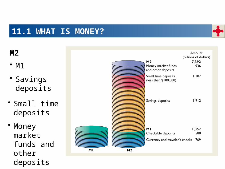
11.1 WHAT IS MONEY?
• Savings deposits
M2
• M1
• Money market funds and other deposits
• Small time deposits

The U.S. Dollar Abroad
The figure shows the growth of U.S. dollars held in the United States
and held abroad
The total quantity of dollar bills in circulation at the end of 2004 was $700 billion.
Edition 3
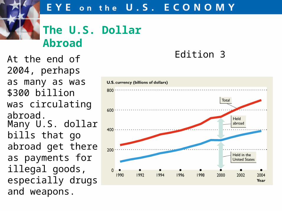
At the end of 2004, perhaps as many as was $300 billion was circulating abroad.
The U.S. Dollar Abroad
Many U.S. dollar bills that go abroad get there as payments for illegal goods, especially drugs and weapons.
Edition 3

Counterfeit U.S. dollar bills are also in use but newly designed bills that are hard to forge have cut this illegal activity.
The U.S. Dollar Abroad
Edition 3
Credit Cards and Money
Today, 80 percent of U.S. households own a credit card, and most of us use a credit card as a substitute for money.
Each month, most of us pay off some of the outstanding balance but not all of it.
In 2005, 57 percent of credit card holders had an outstanding balance after making their most recent payment, and the average card balance exceeded $5,000.
In 1970, only 20 percent of U.S. households had a credit card.
How has the spread of credit cards affected the amount of money that people hold?

Credit Cards and Money
1. As more people use a credit card,
2. The quantity of M1 as a percentage of GDP has decreased.
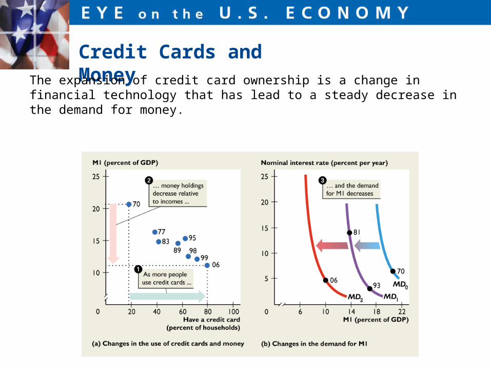
Credit Cards and MoneyThe expansion of credit card ownership is a change in financial technology that has lead to a steady decrease in the demand for money.

http://www.federalreserve.gov/fomc/beigebook/2008/
Fed Watching
2008 January
16
Report
February March
5
HTML
286 KB PDF
April
16
HTML
182 KB PDF
May June
11
HTML
144 KB PDF
July
23
HTML
261 KB PDF
August September
3
HTML
164 KB PDF
October
15
HTML
135 KB PDF
November December
3
HTML
150 KB PDF

An international treaty signed in 1991 required Germany to pay large amounts as compensation for war damage to other countries in Europe.
To meet its obligations, Germany printed money.
The quantity of money in Germany increased by 24 percent in 1921, by 220 percent in 1922, and by 43 billion percent in 1923!
Not surprisingly, the price level increased rapidly.
The figure on the next slide shows how rapidly.
Hyperinflation in Germany in the 1920s

Hyperinflation in Germany in the 1920s
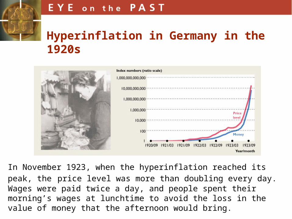
In November 1923, when the hyperinflation reached its peak, the price level was more than doubling every day. Wages were paid twice a day, and people spent their morning’s wages at lunchtime to avoid the loss in the value of money that the afternoon would bring.
Hyperinflation in Germany in the 1920s

In 1923, bank notes were more valuable as fire kindling than as money, and the sight of people burning Reichmarks was a common one.
Hyperinflation in Germany in the 1920s

Ch9
Ch 9 international trade
Andex Charts
Cross relational ECON standards
Web page