Embed Size (px)
Citation preview

Macroeconomics II
Dynamic AD-AS model
Vahagn Jerbashian
Ch. 14 from Mankiw (2010)
Spring 2019
Where we are heading to
I We will incorporate dynamics into the standard AD-AS model
I This will offer another way to analyze economic fluctuationsand the effects of monetary and fiscal policy, e.g.,
I we will use the dynamic AD-AS model to trace out theover-time effects of various exogenous shocks and policychanges on endogenous variables (e.g., Y and π)
I We will show that dynamic AD-AS model can accommodatelong-run economic growth
Dynamic AD-AS model vs. AD-AS model
In contrast to the standard AD-AS model, dynamic AD-AS model
I explicitly incorporates the response of monetary policy to economicconditions (i.e., endogenizes monetary policy)
I It takes into account that CBs set monetary policy accordingto economic conditions, including Y and π
I assumes that CBs set/target the interest rate and allow the moneysupply to adjust to whatever level is necessary to achieve that target
I Previously, we have assumed that CBs set money supply tosimplify the matter
Notes
Notes
Notes

Dynamic AD-AS model vs. AD-AS model
In contrast to the standard AD-AS model, dynamic AD-AS model
I uses inflation rate (but not the price level)
I links subsequent time periods
I Changes in inflation in a period affect future expectedinflation, which changes AS in future periods, which furtherchanges inflation and expected inflation
Dynamic AD-AS model in a few words
Dynamic AD-AS model is
I a very simplified Dynamic, Stochastic, General Equilibrium (DSGE)model
I These models are used in cutting-edge macroeconomic researchin academia and policy institutions such as central banks
I built from familiar concepts: IS curve, Phillips curve, and adaptiveexpectations
I It consists of 5 equations and has 5 endogenous variables: Y ,π, r , i , and πe = Eπ
Notation to incorporate time-dimension
We will use subscripts, "t", to denote time period
I Yt = Real GDP in period t
I Yt+k = Real GDP in period t + k where k ∈ Z
I e.g., if t = 2012 then Yt = Y2012 = Real GDP in 2012
Notes
Notes
Notes
Output: Demand for Goods and Services (IS curve)
In this model demand for goods and services is given by
Yt = Yt − α(rt − ρ) + εt
I Yt is the current output, rt is the real interest, εt is a randomdemand shock (Et−1εt = 0)
I Yt is the "natural" level of output
I For time being we can assume that Yt ≡ Y . Notice howeverthat Yt ↑⇒ Yt ↑
I ρ, α > 0 are parameters
I rt = ρ when Yt = Yt and εt = 0: ρ is the level of "natural"real interest rate
I α shows how sensitive demand is to changes in rt
Output: Demand for Goods and Services (IS curve)
In output equation Yt and rt are negatively related
Yt = Yt − α(rt − ρ) + εt
This is basically our IS curve
I When rt increases firms reduce investments (and consumer’sincrease savings but reduce demand for goods and services)which reduces Yt
The real interest rate: The Fisher equation
The Fisher equation is
rt = it − Etπt+1
I it is the nominal interest rate
I Both rt and it are determined at time t (i.e., their values areknown at time t)
I These are ex ante returns: Returns that people anticipate toearn at time t + 1 on savings made at time t
I πt+1 is inflation in [t, t + 1] period and its value is notknown at time t
I Etπt+1 is the expected inflation given the informationavailable to forecast inflation at time t
Notes
Notes
Notes

Inflation: The Phillips Curve
The Phillips Curve (with output) is
πt = Et−1πt + φ(Yt − Yt
)+ υt
I This is basically SRAS curve where Et−1πt is the previouslyexpected level of inflation
I πt depends on Et−1πt because some firms set prices inadvance
I When they expect high π, they anticipate that their costs willbe rising quickly and that their competitors will be increasingprices and they increase prices
Inflation: The Phillips Curve
Inπt = Et−1πt + φ
(Yt − Yt
)+ υt
I φ > 0 shows how much πt responds when Yt fluctuatesaround its natural level Yt
I When economy is booming, Yt > Yt , firms face higherdemand and higher marginal costs and they increase prices
I υt is exogenous supply shock (Etυt+1 = 0; e.g., oil priceshock)
Expected inflation: Adaptive expectations
For simplicity, we assume people have adaptive expectations
I They expect prices to continue rising at the current inflationrate
Etπt+1 = πt
I This is a significant simplification! It could make sense ifpeople are not sophisticated in forming their expectations
I e.g., with such expectations people do not take into account(understand) that current policy changes affect futureoutcomes such as πt+1
I An alternative could be Rational Expectations
Notes
Notes
Notes

The nominal interest rate: The monetary-policy rule
We assume that the CB sets a target for it based on the deviationof Yt from natural level Yt and πt from targeted level π∗t usingthis rule
it = πt + ρ+ θπ (πt − π∗t ) + θY(Yt − Yt
)I θπ, θY > 0 are parameters
I θπ measures how much the CB adjusts it when πt deviatesfrom its target π∗t
I θY measures how much the CB adjusts it when Yt deviatesfrom its natural level Yt
I This equation is called Taylor Rule
The nominal interest rate: The monetary-policy rule
The CB controls it through open market operations and influencesreal economy through rt
it = πt + ρ+ θπ (πt − π∗t ) + θY(Yt − Yt
)
I e.g., in case when πt > π∗t the CB sells government bonds(i.e., reduces money supply) so that
it ↑⇒ rt ↑ I (rt ) ↓⇒ Yt ↓⇒ πt ↓
I e.g., in case when Yt < Yt the CB buys government bonds(i.e., increases money supply) so that
it ↓⇒ rt ↓ I (rt ) ↑⇒ Yt ↑
Taylor Rule
The hard part of the CBs’job is to choose the target for it andhow much to respond to changes in π and Y
I We have hypothesized a rule. In reality, however, CBs’governing boards do not (need to exactly) follow this formula
I Economist John Taylor proposed a monetary policy rule verysimilar to ours
it = πt + 2.0+ 0.5 (πt − 2.0) + 0.5 (Yt − Yt )
Notes
Notes
Notes

Taylor Rule
The Taylor Rule matches Fed policy fairly well
This figure shows the actual it and the target rate as determined by Taylor Rule
All Equations Together
AD-AS model (in full scale) is
IS : Yt = Yt − α(rt − ρ) + εt
FE : rt = it − Etπt+1AS (PC ) : πt = Et−1πt + φ (Yt − Yt ) + υt
EX (AE ) : Etπt+1 = πt
MP (TR) : it = πt + ρ+ θπ (πt − π∗t ) + θY (Yt − Yt )
Endogenous variables
Endogenous variables of dynamic AD-AS model are
Yt = Output
πt = Inflation
rt = Real interest rate
it = Nominal interest rate
Etπt+1 = Expected inflation
Notes
Notes
Notes

Exogenous variables
Exogenous and predetermined variables of dynamic AD-AS model are
Yt = Natural level of output
π∗t = CB’s target inflation rate
εt = Demand shock
υt = Supply shock
Predetermined:
πt−1 = Previous period’s inflation
Parameters
Parameters of dynamic AD-AS model are
α = Responsiveness of demand (Y ) to r
ρ = Natural rate of interest
φ = Responsiveness of π to Y in the Phillips Curve
θπ = Responsiveness of i to π in the monetary-policy rule
θY = Responsiveness of i to Y in the monetary-policy rule
The model’s long-run equilibrium
Long-run equilibrium: The normal state around which the economyfluctuates
I Two conditions required for long-run equilibrium:
I There are no shocks εt = υt = 0 and inflation is constantπt−1 = πt
Notes
Notes
Notes
The model’s long-run equilibrium
I Combining these conditions with model’s 5 equations givesthe long-run values of endogenous variables
Yt = Ytrt = ρ
πt = π∗tEtπt+1 = π∗tit = ρ+ π∗t
The dynamic AS curve
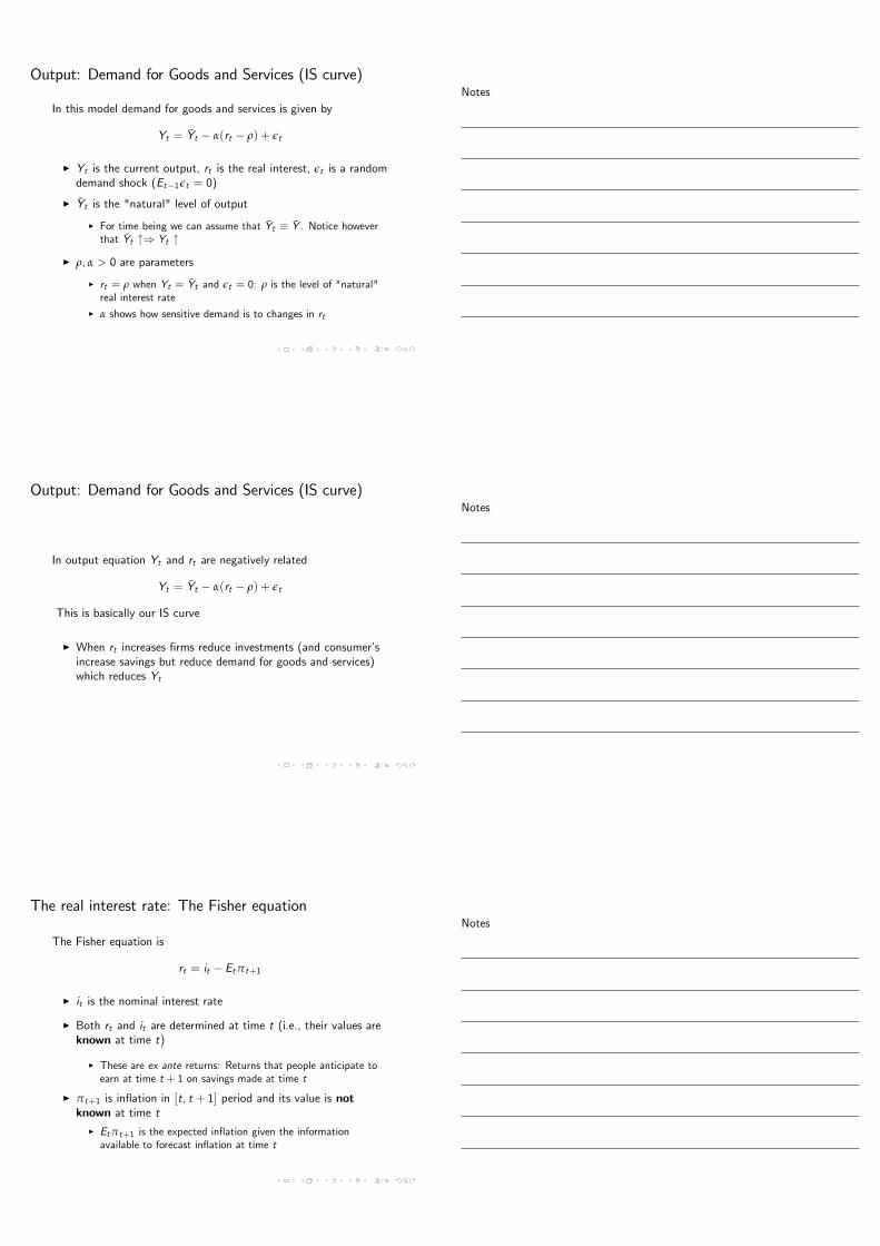
The dynamic AS (DAS) curve combines the Phillips Curve andAdaptive Expectations and shows a relation between Y and π
πt = πt−1 + φ (Yt − Yt ) + υt
On a graph:
The dynamic AS curve
I DAS slopes upward since high levels of output are associatedwith high inflation
I DAS shifts in response to changes in Yt , πt−1, and υt
Notes
Notes
Notes
The dynamic AD curve
The dynamic AD (DAD) curve combines output equation (IS curve),Fisher’s equation, Adaptive Expectations, and monetary-policy (Taylor)rule and shows a relation between Y and π
I From
Yt = Yt − α(rt − ρ) + εt
rt = it − Etπt+1Etπt+1 = πt
it follows that
Yt = Yt − α(it − πt − ρ) + εt
The dynamic AD curve
CombiningYt = Yt − α(it − πt − ρ) + εt
with monetary-policy (Taylor) rule
it = πt + ρ+ θπ (πt − π∗t ) + θY (Yt − Yt )
gives the dynamic AD curve
Yt = Yt − A (πt − π∗t ) + Bεt ,
A =αθπ
1+ αθY,B =
11+ αθY
The dynamic AD curve
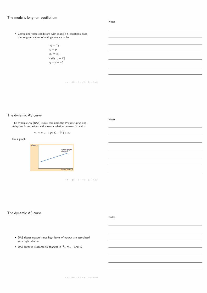
DAD slopes downward
I When inflation rises, the central bank raises r , reducing the demandfor goods and services
I It shifts in response to changes in the Yt , π∗t , and demand shocks εt
I On a graph:
Notes
Notes
Notes

Short-run equilibrium in the modelShort-run equilibrium in dynamic AD-AS model is the combinationof output and inflation that solve the DAD and DAS equations
DAD : Yt = Yt − A (πt − π∗t ) + Bεt
DAS : πt = πt−1 + φ (Yt − Yt ) + υt
On a graph:
Short-run equilibrium in the model
From DAD and DAS equations
DAD : Yt = Yt − A (πt − π∗t ) + Bεt
DAS : πt = πt−1 + φ (Yt − Yt ) + υt
we have the values of Yt and πt
I At time t + 1, πt will become the lagged value of inflation thatinfluences the position of the DAS curve and connecting timeperiods generates dynamic patterns that we will now examine
Long-run growth
Yt changes over-time because of population growth, accumulation ofcapital, and tech-progress
I Since Yt affects DAD and DAS curves in the same way, both curvesshift to the right by the amount that Yt has increased
Notes
Notes
Notes
Long-run growth
Higher Yt implies that
I firms can produce more and DAS shifts to the right
I consumers are richer therefore can consume more and DADshifts to the right
I This is why there is no pressure on inflation
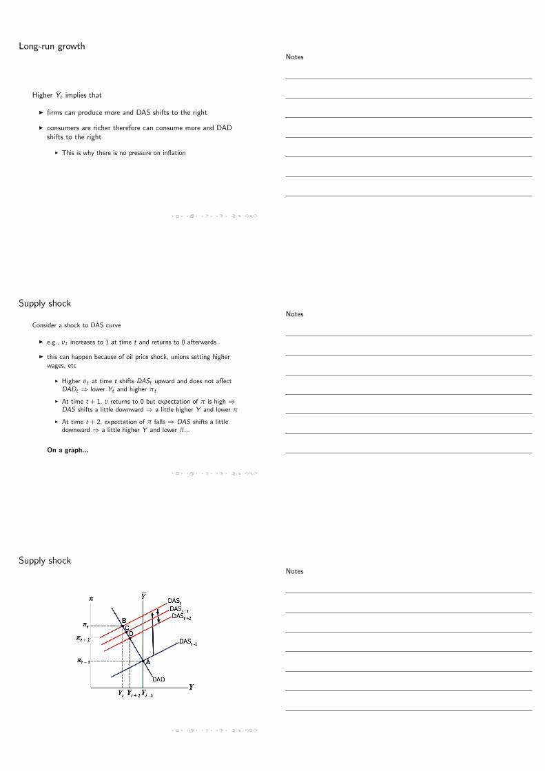
Supply shock
Consider a shock to DAS curve
I e.g., υt increases to 1 at time t and returns to 0 afterwards
I this can happen because of oil price shock, unions setting higherwages, etc
I Higher υt at time t shifts DASt upward and does not affectDADt ⇒ lower Yt and higher πt
I At time t + 1, υ returns to 0 but expectation of π is high ⇒DAS shifts a little downward ⇒ a little higher Y and lower π
I At time t + 2, expectation of π falls ⇒ DAS shifts a littledownward ⇒ a little higher Y and lower π...
On a graph...
Supply shock
Notes
Notes
Notes

Parameter values for simulations
I Yt = 100: Yt − Yt we can interpret as percentage deviation
I π∗t = 2: CB’s inflation target is 2 percent
I α = 1: 1-percentage point increase in r reduces Y by 1percent of its natural level Y
I ρ = 2: natural rate of interest is 2 percent
I φ = 0.25: When Y is 1 percent above Y , π increases by 0.25percentage points
I θπ = 0.5; θY = 0.5: From the Taylor Rule whichapproximates the behavior of the Fed
Dynamic response to a supply shock
The following graphs are called impulse response functions
I They show the dynamic "response" of the endogenousvariables to the shock/"impulse"
Dynamic response to a supply shock
A one-period supply shock affects Y for many periods
Notes
Notes
Notes
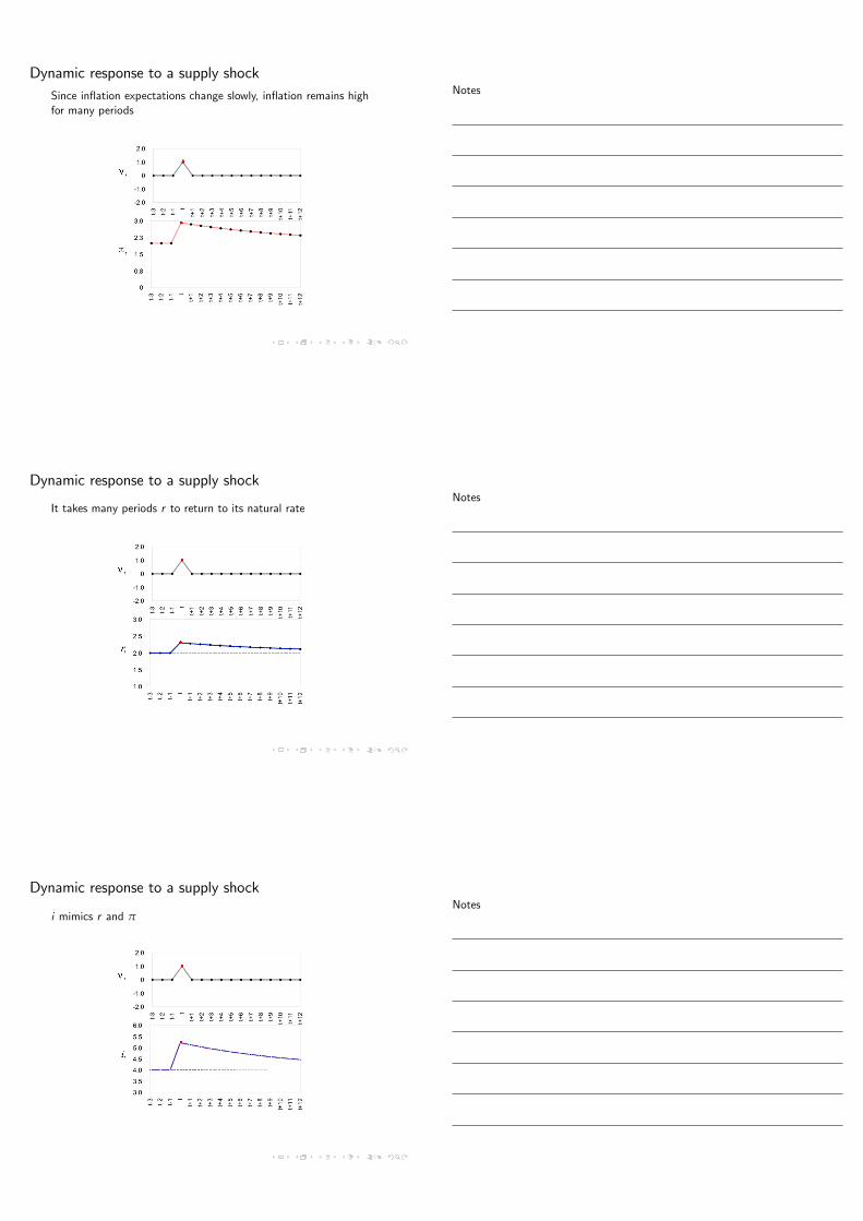
Dynamic response to a supply shockSince inflation expectations change slowly, inflation remains highfor many periods
Dynamic response to a supply shock
It takes many periods r to return to its natural rate
Dynamic response to a supply shock
i mimics r and π
Notes
Notes
Notes
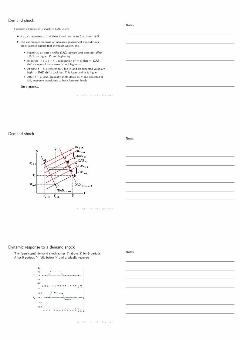
Demand shock
Consider a (persistent) shock to DAD curve
I e.g., εt increases to 1 at time t and returns to 0 at time t + 5
I this can happen because of increases government expenditures,stock market bubble that increases wealth, etc
I Higher εt at time t shifts DADt upward and does not affectDADt ⇒ higher Yt and higher πt
I In period [t + 1, t + 4] , expectation of π is high ⇒ DASshifts a upward ⇒ a lower Y and higher π
I At time t + 5, ε returns to 0 but π and its expected value arehigh ⇒ DAD shifts back but Y is lower and π is higher
I After t + 5, DAS gradually shifts down as π and expected πfall, economy transitions to back long-run levels
On a graph...
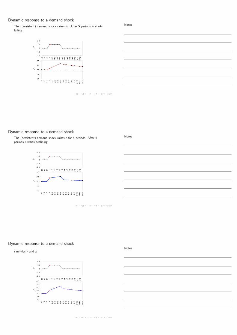
Demand shock
Dynamic response to a demand shockThe (persistent) demand shock raises Y above Y for 5 periods.After 5 periods Y falls below Y and gradually recovers
Notes
Notes
Notes
Dynamic response to a demand shockThe (persistent) demand shock raises π. After 5 periods π startsfalling
Dynamic response to a demand shockThe (persistent) demand shock raises r for 5 periods. After 5periods r starts declining
Dynamic response to a demand shock
i mimics r and π
Notes
Notes
Notes
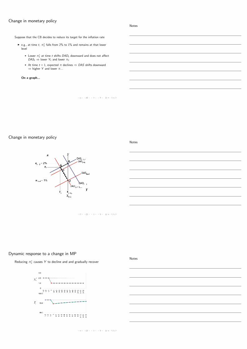
Change in monetary policy
Suppose that the CB decides to reduce its target for the inflation rate
I e.g., at time t, π∗t falls from 2% to 1% and remains at that lowerlevel
I Lower π∗t at time t shifts DADt downward and does not affectDASt ⇒ lower Yt and lower πt
I At time t + 1, expected π declines ⇒ DAS shifts downward⇒ higher Y and lower π...
On a graph...
Change in monetary policy
Dynamic response to a change in MP
Reducing π∗t causes Y to decline and and gradually recover
Notes
Notes
Notes
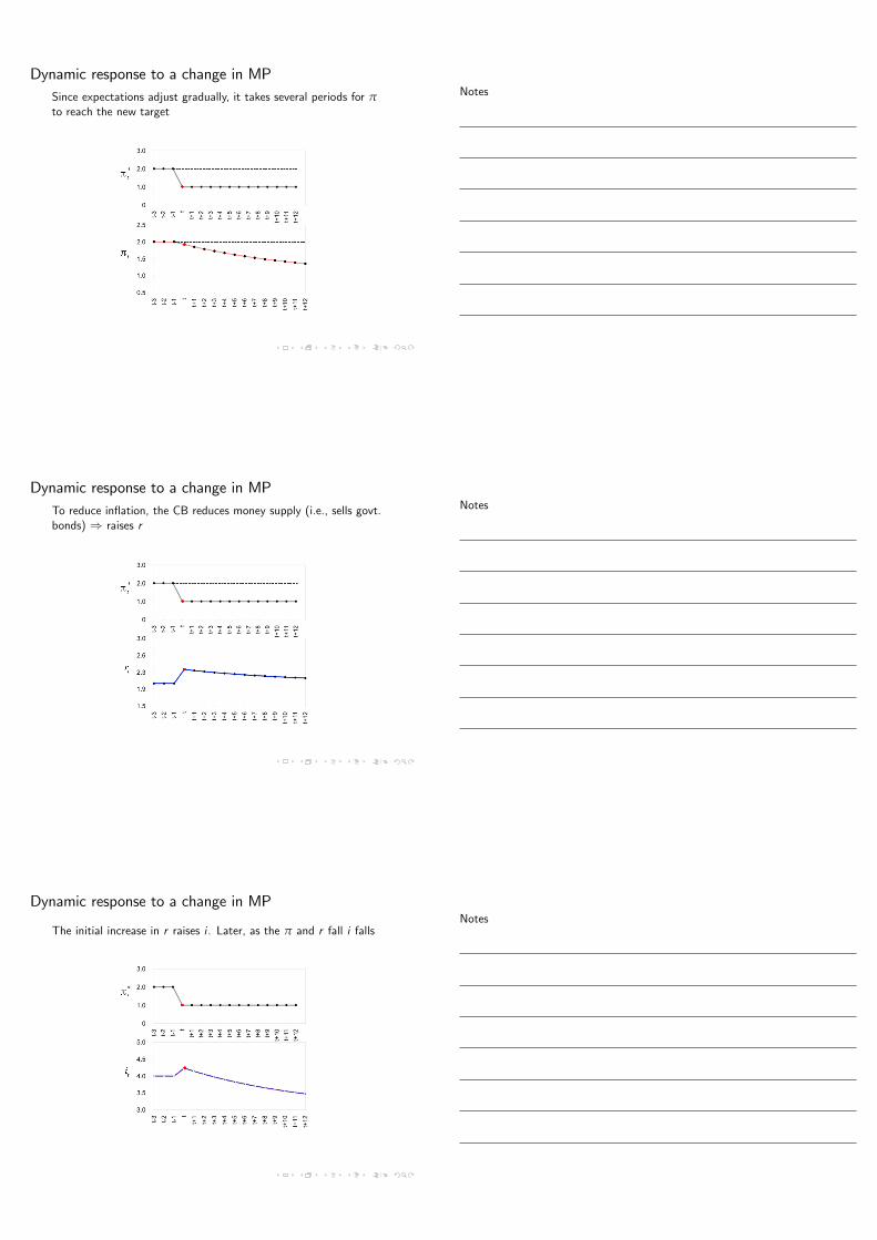
Dynamic response to a change in MPSince expectations adjust gradually, it takes several periods for πto reach the new target
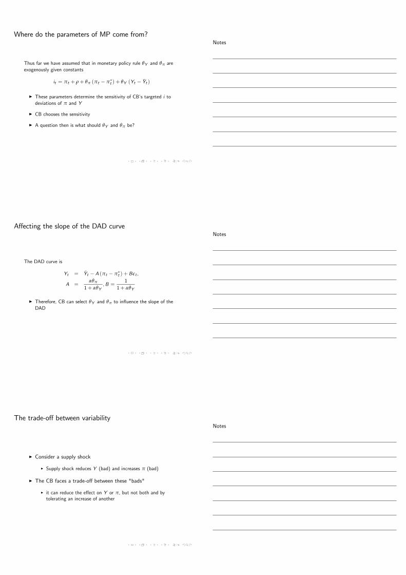
Dynamic response to a change in MPTo reduce inflation, the CB reduces money supply (i.e., sells govt.bonds) ⇒ raises r
Dynamic response to a change in MP
The initial increase in r raises i . Later, as the π and r fall i falls
Notes
Notes
Notes
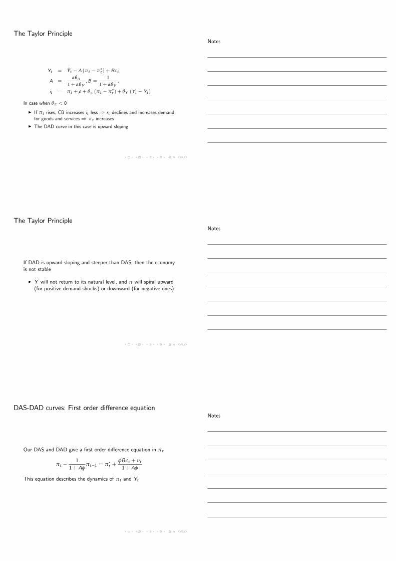
Where do the parameters of MP come from?
Thus far we have assumed that in monetary policy rule θY and θπ areexogenously given constants
it = πt + ρ+ θπ (πt − π∗t ) + θY (Yt − Yt )
I These parameters determine the sensitivity of CB’s targeted i todeviations of π and Y
I CB chooses the sensitivity
I A question then is what should θY and θπ be?
Affecting the slope of the DAD curve
The DAD curve is
Yt = Yt − A (πt − π∗t ) + Bεt ,
A =αθπ
1+ αθY,B =
11+ αθY
I Therefore, CB can select θY and θπ to influence the slope of theDAD
The trade-off between variability
I Consider a supply shock
I Supply shock reduces Y (bad) and increases π (bad)
I The CB faces a trade-off between these "bads"
I it can reduce the effect on Y or π, but not both and bytolerating an increase of another
Notes
Notes
Notes

The trade-off between variability
Case 1: θπ is large and θY is small Case 2: θπ is small and θY is large
I In Case 1 changes in π have big effects on Y ⇒ DAD is flatter
I Supply shocks have a large effect on Y , but small effect on π
I In Case 2 changes in π have small effects on Y ⇒ DAD is steeper
I Supply shocks have a small effect on Y , but large effect on π
The Taylor Principle
The Taylor Principle (named after economist John Taylor) is aproposition that
I CBs should respond to an increase in π with an even greaterincrease in i (so that r rises)
I i.e., CBs should set θπ > 0
I Otherwise, DAD will slope upward
I In such a case economy may be unstable and inflation may getout of control
The Taylor Principle
Yt = Yt − A (πt − π∗t ) + Bεt ,
A =αθπ
1+ αθY,B =
11+ αθY
,
it = πt + ρ+ θπ (πt − π∗t ) + θY (Yt − Yt )
In case when θπ > 0
I If πt rises, CB increases it even more ⇒ rt rises and reducesdemand for goods and services ⇒ πt declines
I The DAD curve in this case is downward sloping
Notes
Notes
Notes
The Taylor Principle
Yt = Yt − A (πt − π∗t ) + Bεt ,
A =αθπ
1+ αθY,B =
11+ αθY
,
it = πt + ρ+ θπ (πt − π∗t ) + θY (Yt − Yt )
In case when θπ < 0
I If πt rises, CB increases it less ⇒ rt declines and increases demandfor goods and services ⇒ πt increases
I The DAD curve in this case is upward sloping
The Taylor Principle
If DAD is upward-sloping and steeper than DAS, then the economyis not stable
I Y will not return to its natural level, and π will spiral upward(for positive demand shocks) or downward (for negative ones)
DAS-DAD curves: First order difference equation
Our DAS and DAD give a first order difference equation in πt
πt −1
1+ Aφπt−1 = π∗t +
φBεt + υt1+ Aφ
This equation describes the dynamics of πt and Yt
Notes
Notes
Notes
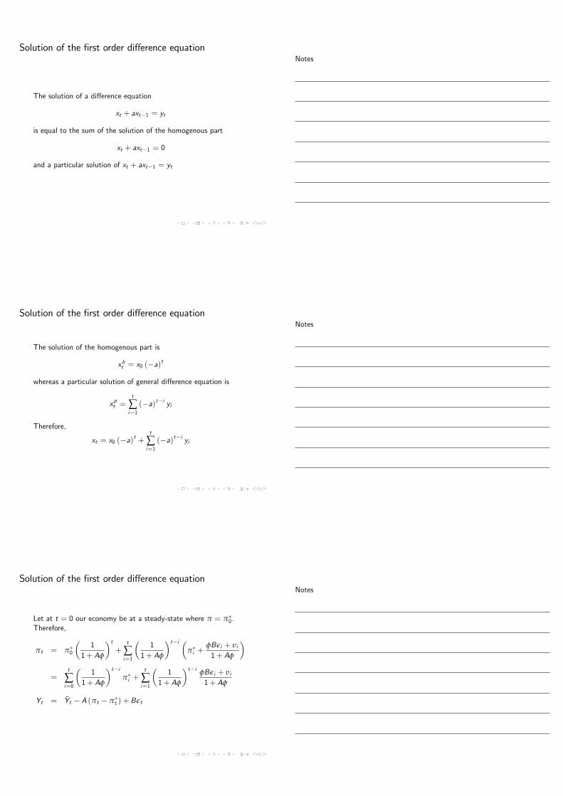
Solution of the first order difference equation
The solution of a difference equation
xt + axt−1 = yt
is equal to the sum of the solution of the homogenous part
xt + axt−1 = 0
and a particular solution of xt + axt−1 = yt
Solution of the first order difference equation
The solution of the homogenous part is
xht = x0 (−a)t
whereas a particular solution of general difference equation is
xpt =t
∑i=1(−a)t−i yi
Therefore,
xt = x0 (−a)t +t
∑i=1(−a)t−i yi
Solution of the first order difference equation
Let at t = 0 our economy be at a steady-state where π = π∗0.Therefore,
πt = π∗0
(1
1+ Aφ
)t+
t
∑i=1
(1
1+ Aφ
)t−i (π∗i +
φBεi + υi1+ Aφ
)
=t
∑i=0
(1
1+ Aφ
)t−iπ∗i +
t
∑i=1
(1
1+ Aφ
)t−i φBεi + υi1+ Aφ
Yt = Yt − A (πt − π∗t ) + Bεt
Notes
Notes
Notes