Mad River TMDLs for Sediment and Turbidity Comment Responsiveness Summary

US Environmental Protection Agency, Region 9 San Francisco, California

December 21, 2007

Commentors:

Bill Elliot, PE, PhD, United States Forest Service Patrick Higgins, Environmental Protection Information Center Tyrone Kelley, United States Forest Service Michael Long, United States Fish and Wildlife Service Tharon O’Dell, Green Diamond Resource Company Carol Rische, Humboldt Bay Municipal Water District Ed Voice and Family, Interested Party

EXECUTIVE SUMMARY

This document summarizes public comments that were submitted to EPA for the Mad River TMDLs for Sediment and Turbidity, identifies the commentor, and responds to those comments. The summary of comments and responses is arranged by commentor. When multiple comments were received on a single topic, the response generally refers to the most extensive comment. Any change that is made to the TMDL document in response to the comment is summarized in the response. If no change is noted in the response, then no change was deemed necessary to the TMDLs.

Summary of Changes to the Final TMDLs

Several changes were made to the final document as a result of public comments. These include: • Various editorial changes and clarification of details regarding sediment and turbidity

issues, the role of the Humboldt Bay Municipal Water District (HBMWD), and current information on the status of salmonid species.

• Additional implementation and monitoring recommendations and additional background information, such as possibilities for prioritizing sediment reduction in coordination with efforts to protect salmonid-bearing streams; acknowledging NMFS’ salmonid recovery strategies and the Mad River watershed group; identifying gravel mining and timber harvesting concerns; discussing future information needs; and describing the Regional Water Board’s role in future revisions of implementation efforts.

• Text to address the western snowy plover, a FWS-listed species in the Mad River area that nests on gravel bars.

• Updated information on Chinook, steelhead, and coho, including the effects of turbidity.

1

• Explanations and results of the revised Sediment Source Analysis (Appendix A to the TMDL document), including modeling used to determine existing sediment loading and set the sediment and turbidity TMDL. The modeling was revised to incorporate more accurate information, and the TMDLs and allocations were revised accordingly. The revised modeling is summarized in the Final TMDL document and below. Additional detail can be found in the revised Sediment Source Analysis (Appendix A to the TMDL document), and in responses to specific comments within this document.

• Tables 1 through 3 (at the end of this document) show the changes to the sediment budget (Table 1) and the sediment and suspended sediment TMDLs as a result of the revisions to the SSA (Tables 2 and 3).

Consideration of Public Comments Leading to the Revised Sediment Source Analysis The vast majority of comments that EPA received addressed the Sediment Source Analysis (SSA), either directly or indirectly. The comments covered a wide range of topics, many of them critical of the sediment source analysis and how it was used to set the TMDLs. Some of the comments were supportive of the analysis and TMDLs. A number of comments reflected confusion about how the SSA was developed, how tasks were undertaken for the SSA, and how the information presented in the SSA was used (or not used) in the TMDL document and in setting the TMDLs. EPA carefully considered all of these comments and decided to revise the SSA, incorporating most of the suggestions that were provided. EPA agreed with the concerns that led us to revise the SSA and TMDLs to reflect these improvements. Although re-running the models and revising the SSA is no small undertaking, particularly given that EPA is obligated to establish these TMDLs within a Consent Decree deadline of December 31, 2007 (see TMDL document, Chapter 1), we believe that the revisions led to an improved SSA and TMDL document, and it has improved our confidence in the analysis and in setting the TMDLs.

Separate from the changes to the SSA and TMDLs is the issue of clarifying the SSA and TMDLs. Some of the public comments expressed confusion directly and asked for explanations or clarifications. Some of the criticisms simply reflect a misunderstanding of the methods in developing the SSA and setting the TMDLs. EPA reviewed these concerns and concluded that the descriptions of what was done would benefit from improved clarity, as is discussed in more detail below.

The SSA is complex, as it covers a very large watershed (nearly 500 mi2), and, for the most part, utilized existing information. New information was developed specifically to address turbidity issues and to develop supportable relationships between turbidity and suspended sediment concentration (SSC), in order to set TMDLs for turbidity as well as for sediment. Moreover, the SSA utilizes two separate models, including the Watershed Erosion and Prediction Project (WEPP) Road Batch (Elliot et. al., 2000) to estimate road-related surface erosion, and NetMap to estimate hillslope creep and fluvial erosion. Field reconnaissance informed both the WEPP and NetMap model inputs. Inputs from measured suspended sediment concentrations in the Mad River basin and from the WEPP analysis were used in NetMap. The landslide analysis, which utilized both desktop (air photo analysis) and field verification components, also provided information for the NetMap model. GMA developed a traditional sediment budget for this analysis, similar to those developed for other TMDLs, but we developed additional information primarily because these are the first turbidity TMDLs that have been developed for California’s

2

North Coast. In this effort, we developed some information that was eventually determined not to be useful for the scale of the analysis.

Both WEPP and NetMap provide inputs to the development of the sediment budget, which is used to set the TMDLs. NetMap is capable of predicting average annual sediment load that is routed through the system, and identifying sediment production at specific locations throughout the watershed. This use is beyond the scope of the task of setting sediment and turbidity TMDLs, but the NetMap sediment budget was used to provide a check on the accuracy of our sediment budget, and we compared the results with our measured sediment loads. In the original SSA (GMA, 2007a, Appendix A to the draft TMDLs) and draft TMDLs, the two methods did not correlate well, and we relied upon the traditional sediment budget. The public comments pointed out ways that our assumptions could be improved, which were corrected in the revised SSA and TMDLs. With these revisions, the two sediment budgets are in closer agreement. Yet there remain fundamental differences between the two types of models, and their sediment load predictions are not directly comparable.

The models themselves are complex, input data sets are very large, and the use of the models in developing the SSA and setting the TMDLs is complex. Simplifying the explanation of the SSA methods and the use of the SSA data in setting the TMDLs in a way that is easy to understand yet technically complete is a considerable challenge. Responding to most of the comments would require repeating these explanations many times. In addition, there are some commentors who supported the original analysis and TMDLs. EPA feels confident that the revisions have improved the SSA and TMDL document. Additionally, we determined that it would be most effective and much less confusing to all if we summarize the SSA and methods of setting the TMDLs, including the resulting revisions, in this document (see next section). Thus, we are maintaining transparency in the public process and communicating the revisions as clearly as possible.

Accordingly, the next section summarizes the revised SSA, which is Appendix A to the TMDL document. Following this, individual comments and EPA’s responses are summarized. Many of the responses refer the reader back to the SSA Summary, the TMDL document or the SSA itself for further explanation as needed.

Graham Matthews Associates (GMA) developed the SSA for EPA. EPA reviewed GMA’s methods and results, and both GMA and EPA are confident that the revised results reflect the best information currently available for setting the TMDLs. This analysis is conducted at the basin-wide scale (nearly 500 mi2), and may not be adequate for site-specific project analyses, such as timber sales. However, it is possible to build upon this information, improving the specificity or making use of new information available in the future to develop project-specific information, or to investigate other watershed-wide needs. EPA encourages this use, and encourages both private and public organizations to work with the Regional Water Board to facilitate and improve upon its implementation efforts in the future.

Sediment Source Analysis Summary The sediment source analysis consists of several components: 1) a landslide analysis; 2) suspended sediment and turbidity monitoring; 3) Watershed Erosion and Prediction Project

3

(WEPP) modeling; and 4) NetMap modeling. Because the development of the sediment source inventory is complex, and because the components are both complex and interconnected, we will summarize it here. Additional detail can be found in the revised SSA document (Appendix A of the TMDL document). Table 1 (at the end of this document) summarizes the changes to the sediment budget and Tables 2 and 3 (also at the end of this document) summarize revisions between the draft and final TMDLs for sediment and suspended sediment, as well as the revisions to the TMDL document incorporate these changes.

The sediment source analysis accounts for chronic and episodic sediment input to the stream network. Data were derived from the US Geological Survey (USGS), US Forest Service (USFS), California Department of Water Resources (DWR), Humboldt Bay Municipal Water District (HBMWD), the Blue Lake Rancheria (BWR), Green Diamond Resource Company, Inc. (GD), Klein (2006, unpublished, in the SSA), and monitoring data collection and analysis by EPA’s contractor, Graham Matthews Associates (GMA). Additional information from the Washington State Watershed Analysis Manual (WDNR, 1995), for similar geologies, was used to refine some assumptions, where existing data were inadequate. The SSA characterizes the sediment conditions of the watershed and develops a sediment budget, from which the TMDLs are set.

Sediment Budget Categories The sediment budget breaks the components of sediment production into three categories of natural, or background, sediment (background creep, background landslides, and bank erosion); and four categories of management-related sediment (road-related and timber harvest-related landslides and surface erosion). The draft TMDLs aggregated background creep, derived from both dormant (slow-moving) and active (fast-moving) earthflows, together with bank erosion. For the Final TMDLs, we have separated those two sources. These were developed using the NetMap model.

Landslide Analysis The landslide air photo assessment was conducted for all land in the watershed, including the USFS lands of the Six Rivers National Forest and private lands. Some information, particularly for small sources, was not available for private lands. GMA summarized and compiled data from the California Department of Water Resources (DWR, 1982), California Department of Mines and Geology (DMG, 1999), Green Diamond Resources, Inc. (GD, 2006), and USDA, Forest Service (USFS) landslide data. The DWR (1982) data is the most comprehensive map and covers the entire Mad River from 1974 aerial photographs. The DMG (1999) data covers the lower watershed, and the USFS data covers the upper and middle watershed. The GD data covers a limited portion of the middle and lower watershed. Dormant and active landslides were included in the landslide database. Active pre-1975 landslides mapped by CDWR (1982) were used to create the pre-1975 active landslide map. The post-1975 landslide map includes data from all of the sources listed above in addition to landslides mapped as part of this study. Like DWR (1982), GMA mapped active landslides with obvious activity from the most recent sets of remote sensing data (i.e., 2003 aerial photographs and 2005 digital ortho photographs). For all lands, existing active landslide maps were reviewed and incorporated into the GMA landslide map as deemed appropriate. For USFS lands, publicly available aerial photographs were used,

4

and on private lands the digital orthophotographs and hillslope relief maps were used to map active landslides.

Landslides that were initiated or enlarged between 1975 and 2003/2005 were mapped as contributing to the sediment budget from 1976-2006. A portion of the mapped landslides was field checked to validate the desktop evaluation, and to determine depth/volume relationships and other factors. Although approximately 15% of the landslides were field checked, the extent of the field work was limited by access: for example, if landowners denied entry, steep topography, or roadless areas prevented travel, or active logging operations were underway. For the Final TMDLs, several changes were made in response to public comments. This included reviewing some landslide features to determine whether management associations were correct and changing assumptions for road-related causes. In the draft, roads within 100 ft of a landslide feature were assumed to be associated with the landslide without field verifying causal links; for the final, only roads that actually crossed a landslide feature were determined to be associated with that feature. The database was re-examined for this process as well, to ensure that no landslides were inadvertently reclassified as having natural causes. As a result, six features were reclassified from road-related to natural causes.

Area/volume relationships were also re-examined. Using the database of field-verified landslide areas and volumes, we examined the statistical relationship between depth and area, and found a strong correlation. However, when we applied this approach to the remainder of the database, it suggested unreasonably high sediment delivery rates, similar to those found in very active terrain in New Zealand, but not found in the North Coast. We determined that the number of extremely large, deep-seated slides that were field-verified, was disproportionately high, throwing off the correlation. Accordingly, we adjusted the area/volume relationships, based on the assumption that the relationships would not reasonably yield volumes higher than the Redwood Creek watershed adjacent to the Mad River basin. These changes resulted in some increases and some decreases to the sediment loads of both natural and management-related landslides, depending on the landslide type and size: volumes of large landslides were previously underestimated, because the assumed landslide depth was too small to be representative; and volumes of smaller landslides were overestimated, because the assumed landslide depth was too large. Additional area/depth relationships that more accurately represented the various types of landslides improved the landslide volume estimates overall.

Suspended Sediment and Turbidity Monitoring

Turbidity and suspended-sediment concentration (SSC) data were collected at several monitoring sites to characterize the watershed, and were analyzed by developing relationships for SSC versus turbidity and SSC versus discharge for all sites. Suspended-sediment discharge and load estimates were computed using either turbidity or discharge as a surrogate for suspended-sediment concentration, based on the developed correlations. This was used to identify which areas of the Mad River basin are more or less disturbed, and it allowed us to estimate sediment loads in each subarea based on the measured data. These estimates were also used to calibrate the NetMap model (described below). Perhaps most importantly, the strongly-correlated relationships developed between turbidity and SSC allowed us to set the TMDLs as suspended sediment loads.

5

WEPP Modeling

The most significant change in the sediment source analysis and TMDLs between the draft and the final was made in the Watershed Erosion and Prediction Project (WEPP) modeling, which was used to generate the road surface erosion and the harvest-related surface erosion, as well as to provide input into the NetMap model, which was used primarily to estimate fluvial erosion and hillslope creep, as described below. Two commentors took exception to our modeling assumptions and results in the draft analysis. WEPP is known to overestimate sediment production, and the results from our initial analysis showed that road-related surface erosion was extremely high.

GMA consulted with Bill Elliot, of the USFS Intermountain Research Station, who was one of WEPP’s developers. Our roads database, which is the best available to date, does not have complete information on road parameters other than surface type. Many variables influence sediment delivery to streams from roads: surface type, level of use and maintenance, geology and topography, hillslope position (e.g., ridge top versus canyon bottom), road drainage, stream crossings, and road prism types, for example. Based on Elliot’s recommendations, we ran the model several times with varied assumptions, and determined that the main parameter driving the model was whether the inboard ditch was vegetated or unvegetated. In our draft analysis, we assumed that all roads were constructed with an inboard, unvegetated ditch. This was a worst-case, conservative assumption, which we realized would overestimate road-related surface erosion. We used this in the absence of better data, in order to err on the side of caution. However, in considering the public comments that the erosion was significantly overestimated, and in considering that the estimates were greater than our measured sediment yield estimates by a factor of four, we determined that it was appropriate to re-run the model using broader assumptions. For the final, we ran the model assuming that roads had vegetated inboard ditches (again, in consultation with Elliot). Even this appeared to over-predict sediment, so we also set an upper threshold for road-related surface erosion based on the Washington State Manual (WA DNR, 1995), based on similar soil and climate types.

These changes resulted in reductions to the estimates of road-related surface erosion between the draft and final TMDLs, by about 55% overall. The reductions ranged from a high of 83% in the Upper Mad subarea, where most roads are ridgetop roads that contribute far less erosion to streams, to a low of 48% in the Lower/North Fork subarea, where miles of roads and road densities are greatest. Some uncertainty remains in the roads database and in the WEPP model itself, but EPA is confident that the revisions result in a closer prediction of road-related erosion. Road-related erosion still comprises the bulk of the average annual management-related erosion: 62% of sediment production basinwide is associated with roads, and only 2% of sediment production is associated with timber harvest, while 36% is thought to be associated with natural causes, primarily associated with unstable Franciscan mélange.

NetMap Modeling

NetMap is a complex tool used for watershed characterization and sediment budgeting. For the Mad River TMDLs, NetMap was used to develop estimates of background surface erosion (creep from active and inactive, or slow-moving, earthflows), bank erosion, and for watershed characterization (topographic indices, Digital Elevation Models, or DEMs, developing mean

6

annual flow, and channel classification). In the traditional sediment budget portion of the SSA, it contributes the estimates of background creep and bank erosion.

NetMap can be used to develop a sediment budget at the smallest scale (e.g., a GIS pixel) in the watershed; the program models the delivery of that sediment to the stream and the routing of that sediment through the stream system. EPA had originally expected to use GMA’s NetMap model to develop the sediment budget; however, several problems were encountered. For example, as described in the original SSA and draft TMDL, the results of the NetMap sediment budget diverged widely from the sediment yield estimates derived from measured suspended sediment concentration (SSC) and associated suspended sediment load (SSL) estimates. Accordingly, the SSA relies primarily on the development of a traditional sediment budget to estimate sediment production and delivery to the stream system in the Mad River basin since these results matched the measured values more closely. EPA revised the text in the final TMDL document to distinguish between what NetMap was used for (contributing creep and bank erosion to the traditional sediment budget, and assisting with watershed characterization) and what it possibly could be used for in the future (e.g., developing sediment budgets based on different design flows, for example, and targeting areas for watershed improvement). We also included text in Chapter 4 to suggest its further development and use as a tool for implementation.

Two methods were used to model NetMap for the Mad River basin. The first uses a Generic Erosion Potential, or GEP. It is based on the DEM, and factors in topographic slope (steepness) and slope convergence, which are two factors that are known to contribute to the initiation of landslides, surface, and fluvial erosion. This method does not work well in hummocky terrain, such as the large landslide-prone, earthflow terrain comprised of unstable Franciscan and Schist found in parts of the Mad River basin. GEP is driven by slope convergence, which is not an equally strong factor in earthflow terrain. These areas are driven more by other factors. Thus, for these terrains, NetMap is used without GEP. The second method uses a modified GEP developed from average sediment delivery by slide type and geology.

The final SSA and TMDL document use revised inputs to NetMap based on other revisions to the SSA inputs. For example, NetMap uses surface erosion estimates from the WEPP model to modify the GEP in the NetMap model. It also uses the revised area/volume relationships developed in the landslide analysis. The revised assumptions are probably a reason that the NetMap results are now much closer to the monitored results (see Appendix A).

Because it can be used to develop a sediment budget based on different flood flows, NetMap is used in the SSA (and in the TMDL) to illustrate the differences in sediment delivery between a small storm and a less frequent storm, and can account for the effects of the reservoir; Figure 10 in the TMDL and Figure 44 in Appendix A show this relationship between background and existing sediment load for an average water year. While this part of NetMap is used in the TMDL document simply to characterize the watershed and illustrate the differences between acute and chronic storm flows, this is also essentially one of the initial steps that can be taken to further develop NetMap to refine the sediment budget in the future, if that is desired by the Regional Water Board or other organizations in the implementation phase.

7

SUMMARY OF COMMENTS AND RESPONSES

Commentor 1: Bill Elliot, PE, PhD, United States Forest Service

These comments were also included as Attachment A for Commentor 3 (Tyrone Kelley, United States Forest Service). Responses to these comments are included in Comments 3-1, and 3-31 to 3-34.

Commentor 2: Patrick Higgins, Consulting Fisheries Biologist for Environmental Protection Information Center

Comment 2-1: The Draft [TMDLs] “appear technically sound and properly assign a substantial pollution load to land use activity, particularly logging and associated road building. The U.S. Environmental Protection Agency is to be commended for funding collection of sediment transport and turbidity data to plug data gaps and to truly assess the magnitude and origin of the Mad River sediment pollution problem. The Draft [TMDLs] set appropriate targets for indicators of sediment pollution and recommend their use for long term trend monitoring with the only exception being a reluctance to set a numeric standard for mainstem Mad River turbidity.”

Response: The commentor’s reference to “numeric standard” is unclear. If the reference is to water quality standards, the Regional Water Board is responsible for setting water quality standards, including standards for turbidity. The numeric standard for turbidity of not more than 20 percent over background levels applies to the mainstem Mad River as well as tributaries. The TMDLs include allocations for turbidity, expressed as suspended sediment. These were set at 20 percent over background levels, consistent with the existing water quality standards. In addition, EPA included a numeric target for turbidity, which was based on analysis of reference streams and was derived from the Regional Water Board’s existing numeric standard for turbidity of not more than 20 percent over background levels. This target, while it is not legally enforceable, should be considered as part of a suite of indicators, and is intended for subwatersheds that are less than 10 mi2 in area. This is found in Section 3.3.2 of the TMDL document.

Given the Regional Water Board’s existing numeric standard for turbidity, and our review of the best available information, EPA does not feel that additional targets are warranted at this time. However, it is possible that the Regional Water Board may consider such information in developing its implementation plan, or during review of water quality standards in the Basin Plan. See also response to Comment 2-10.

Comment 2-2: “EPA defers to the California State Water Resources Control Board on TMDL implementation, but none the less, the final Mad River TMDL needs to be explicit with regard to setting prudent risk thresholds for timber harvest, road densities and the number of road crossings so that further damage from cumulative watershed effects can be prevented. Prioritization for action should reflect a “best science” approach to Pacific salmon restoration

8

similar to that put forth by Bradbury et al. (1995). Alteration of sediment transport processes by gravel mining in the lower Mad River has also compromised attainment of beneficial use with regard to fisheries and the need for changes in gravel management practices needs to be discussed in the final [TMDLs].”

Response: EPA utilized the best available science to develop the Mad River sediment and turbidity TMDLs. The goal of the TMDLs is to determine the loads for sediment and turbidity that will result in attainment of water quality standards for those pollutants. While restoration of Pacific salmon stocks may be a result of attainment of water quality standards, population recovery is not guaranteed, due to other factors beyond the scope of these TMDLs (e.g. ocean conditions, commercial fishing, etc.). EPA believes that setting risk thresholds for timber harvest, road densities, and the number of road crossings may be a part of an appropriate implementation plan, which should be developed by the Regional Water Board. Similarly, calling for specific changes in gravel management practices would be appropriate within an implementation plan. The Humboldt County Planning Department, which sets policies for gravel mining within Humboldt County, is currently developing a Supplemental Programmatic Environmental Impact Report (PEIR) for gravel mining to address an adaptive management strategy based on mean annual gravel recruitment. Text regarding salmon, including recovery efforts by NMFS, and text regarding gravel management, has been added to the document. See also response to Comment 7-1.

Comment 2-3: “While the Draft TMDL recognize overall declines in Pacific salmon species populations, there is no recognition that some species like coho salmon may go extinct, if emergency action to remediate pollution is not implemented. The [TMDLs] need to specifically stress preventing pollution immediately in sub-basins critical to coho salmon recovery.

Response: EPA shares the concerns for the salmon population, and we have added additional text to Chapter 2 to summarize the current status of Pacific salmon species, according to the most recent information available from NMFS. Additional text has also been added to Chapter 4: to emphasize recovery efforts underway and under development by NMFS; to suggest that the Regional Water Board consider implementation prioritization by subwatersheds that currently support salmon stocks; and to encourage cooperative efforts by the many different agencies and organizations responsible for watershed improvements and species recovery.

Comment 2-4: Components of the TMDLs are described, and the consequences of cumulative watershed effects are discussed. “The final Mad River TMDL[s] should specifically note the prior failure of the timber harvest review process to prevent water pollution, loss of fish habitat and the decline of Pacific salmon and call for a change in approach to future timber harvest oversight to reverse these problems.”

Response: EPA is not responsible for timber harvest regulations, and has not specifically analyzed the effectiveness of those regulations in achieving water quality standards in the Mad River basin; however, the document recognizes that salmonids have continued to decline, and that sediment from roads and landslides, some of which is related to timber harvest, is responsible for much of the excess sediment and turbidity. Text that was added

9

regarding Pacific salmon stocks also acknowledges NMFS’ identification of the contribution of forestry activities to declines in the populations, and adds that NMFS will continue to work toward recovery with the Board of Forestry, as well as with other agencies.

Comment 2-5: “Age class data provided as part of the Simpson Timber (2002) Coho Salmon Habitat Conservation Plan indicates that timber stands in the Mad River and North Fork Mad River are primarily early seral stage, indicating a very rapid rate of recent logging (Figure 2). The aerial image shown as Figure 3 shows that timber harvest within the Lindsay Creek watershed is approaching or exceeding the threshold recognized by Reeves et al. (1993) as causing damage to fish habitat and a decline of pacific salmon species diversity. The Draft TMDLs mention that Lindsay Creek is one of the last of Mad River Tributaries supporting coho salmon, but makes no recommendation regarding limiting further timber harvest in this sensitive watershed or elsewhere.

Response: The Regional Water Board may determine, in its implementation plan, that limiting timber harvest is appropriate in the Lindsay Creek subwatershed. EPA has set allocations by subarea (Lindsay Creek is in the Lower/North Fork subarea) and source (e.g., timber harvest and roads). The actions taken to achieve those loads are the responsibility of the Regional Water Board. Additional text has also been added to Chapter 4 to emphasize the urgency of recovery in watersheds that support endangered salmonid populations such as coho.

Comment 2-6: “Cedarholm et al. (1981) found that road densities greater 4.2 miles (mi) of road per square mile (mi2) of watershed yielded sediment levels 260% to 430% over background and increased fine sediment in salmon spawning gravels by 2.5 – 4.3 times. U.S. Forest Service (1996) studies in the interior Columbia River basin found that bull trout were not found in basins with road densities greater than 1.7 mi/mi2. They ranked road-related cumulative effects risk as Extreme when road densities exceed 4.7 mi/mi2 (Figure 4). National Marine Fisheries Service (1996) guidelines for salmon habitat characterize watersheds with road densities greater than 2.5 mi/mi2 as “Not Properly Functioning” while “Properly Functioning Condition” is defined as less than or equal to 2 mi/mi2 with no or few stream side roads. The Draft TMDLs indicate that the Mad River watershed as a whole has 4.6 miles of road per square mile of watershed and densities as much higher in sub-basins with recent, active timber harvest (Figure 5). This level of road density is well above thresholds known to cause sediment and flow related cumulative watershed effects. Figure 6 shows high road density in Canon Creek in the Middle Mad River sub-basin. Armentrout et al. (1999) recommended no more than 1.5 crossings per mile of stream to lessen the risk of cumulative effects in major storms.

Response: EPA acknowledges in the TMDL document that road densities in some subwatersheds are very high, averaging 4.2 mi/mi2 in the basin as a whole (not 4.6 miles; the commentor may have misread the document). The highest road densities are in the Lower/North Fork Mad River subarea, averaging 7.5 mi/mi2. Cannon Creek, which is in the Lower/North Fork subarea, is among the subareas with the highest road densities, at 7.0 mi/mi2, of which 6.3 mi/mi2 is native surface roads. The Upper and Middle Mad River subareas, by contrast, average 3.2 and 3.0 mi/mi2, respectively.

10

The TMDLs recognize the contribution of roads to the sediment and turbidity pollution; the draft TMDLs called for a 93 percent reduction in road-related sediment basinwide. As described in the response to Comment 3-1, some of the assumptions used to model the road-related sediment were changed to improve the accuracy of the estimate in response to public comments, which resulted in changes to the estimates of existing road-related sediment and background sediment. Even with those changes, the final TMDLs are set at a level that would need an 89 percent reduction in road-related and other sediment to attain the TMDL goals basinwide. Chapter 4 includes recommendations to prioritize reductions of road-related sediment.

Comment 2-7: “There are several steep inner gorge locations in the Middle Mad sub-basin with old growth forests owned by industrial timber companies that, if logged, may lead to catastrophic failures. The TMDL should recognize this elevated risk and discourage such land use activity in the final.”

Response: Responsibility for implementation plans rests with the Regional Water Board. EPA recognizes that inner gorge areas present greater risk for certain management activities. We have added text to acknowledge that risk, and have expanded the discussion in Chapter 4 for the same reason. However, results of this analysis should not be used for site-specific geotechnical input for landslide prone terrain. Standard site-specific engineering geology methods should be used to evaluate and mitigate the effects of logging on landslide prone areas, especially inner gorge area along the Mad River that are likely some of the most sensitive ground within the watershed.

Comment 2-8: “The changes in Canon Creek following extensive logging demonstrate significant cumulative effects. On a hike to Sweasey Dam in September 1966, I walked lower Canon Creek just above its convergence with the Mad River. Although flow was only slight between pools, the depth within the pools was 4-6 feet and there were numerous salmonid juveniles of several size classes. More than 50% of the watershed was logged from 1980-1995. Pools in lower Canon Creek were obliterated by sediment transport and channel widening killed riparian trees in low gradient response reaches that were formerly extremely productive for spawning and rearing salmonids (Figure 6). The convergence of Canon Creek and the Mad River is occupied by a large delta. I attended a presentation at Humboldt State University in 1999 where a consulting statistician for Simpson Timber reported increases in channel width of Canon Creek from 50 feet to 150 feet wide from 1985-1999. This stream was a coho salmon index stream for the Pacific Fisheries Management Council, but returns have averaged only five coho adults per year after logging (Zuspan and Sparkman, 202). The delta at the mouth was impeding fish during low flows so that adult coho could not enter during dry falls in the early 1990s, but USFWS has since funded a project to restore passage (Golightly, 1998).”

Response: The commentor’s description appears to be consistent with EPA’s estimate of sediment production in the subwatershed. Canon Creek and the North Fork Mad River subareas have the highest unit road-related surface erosion rates in the basin: 583 and 714 tons/mi2/year, respectively, which is close to three times the basinwide average of 242 tons/mi2/year.

11

Comment 2-9: “The turbidity data collected for the Mad River TMDL and the combined analysis with existing data from Klein (2003; 2006) are a major highlight of the report and a significant contribution to regional scientific understanding. The conclusion that ‘turbidity values for the Mad River sites are orders of magnitude greater than the background rates’ is correct and well founded. The Draft TMDL does not sufficiently discuss the implications of the elevated turbidity on Mad River coho salmon and steelhead nor does it set a sufficiently specific target for turbidity. Sigler et al (1984) found that turbidity above 25 nephlometric turbidity units (NTU) inhibited feeding of juvenile coho salmon and steelhead trout juveniles and therefore reduced their growth rates. Most coho and steelhead must spend one or two winters in freshwater, respectively. The NCRWQB (2004) (sic) pointed out that ‘reductions in growth decrease the chance of smolts to mature and return as spawning adults, which cumulatively jeopardizes population sustainability (Trush 2001).’ The extremely high chronic turbidity documented in the Draft TMDL showed that the lower Mad River exceeds 25 FNU (formalin turbidity units) over 80% of the period of record (Figure 7). For assessing the impact to coho and steelhead juvenile growth NTU and FTU (sic) are used interchangeably because there is only a minor difference between these metrics at low levels (0-2) (Randy Klein personal communication).

“In addition, because much of the Lower Mad, North Fork and Middle Mad are in private ownership and intensively managed, there are no lightly managed sub-basins where fish may find refugia of clear water during winter periods of high flow. Collison et al. (2003) characterized this pattern of homogeneous watershed disturbance and distinguished it from natural ‘patch’ disturbance regimes that only affected small areas in varying sub-basins during periodic disturbance from fire, floods or earthquakes. The lack of clear water refugia and extreme, chronic turbidity can be directly linked to coho salmon population falling to levels of fewer than 100 adults annually. The CDFG (Sparkman, 2003) finding that 88% of steelhead in the angler catch are of hatchery origin is consistent with poor survival of wild steelhead juveniles due to highly turbid over-wintering conditions.”

Response: Regarding the turbidity target and water quality standards, please refer to response to Comment 2-1. The response to Comment 2-11 contains additional information on the regional context for extinction risk, for which additional text was added to the document. We have also added additional discussion on the effects of elevated turbidity on salmonids.

Comment 2-10: “Setting a limit of 10% exceedence of the 25 NTU/FTU level should be considered. The Oregon Department of Environmental Quality’s (ODEQ, 2005) exhaustive review of literature on turbidity concurs with Newcombe (2003) that while the duration of exposure is important, 25 NTU should be a benchmark for impairment for salmonids…. The NRCWQCB (2006) acknowledged that the work of Klein (2003) suggests that a threshold for turbidity of a number of days over 27 NTU or a 10% exceedence limit for this value might be appropriate. They also take note of a difference approach suggested by Trush (2001) that would require that the turbidity be below 27 NTU ‘when the measured flow rate is at ten percent of the daily average late-winter baseflows…. This criteria allows reliable measurements for the development of baseflow turbidity rating curves.’”

Response: Please refer to response to Comment 2-1.

12

Comment 2-11: “What the Draft TMDL fails to do is to provide a regional context for extinction risk for species like coho salmon and information on known climate and ocean productivity cycles that will influence recovery…. Any additional loss of populations is extremely undesirable and … recovery of coho without substantial human intervention is unlikely.

“The Draft TMDL states that ‘recent studies conducted during the winter months of 1999-2003 by CDFG estimated only 46 coho salmon in the Mad River (Sparkman 2003),’ but fails to recognize that this represents an extreme risk of loss of the Mad River coho salmon population.

“Summer steelhead are not recognized specifically as a distinct species in the Draft TMDL, but they are a separate stock and qualify as a species under ESA… The summer steelhead population is also at elevated risk of loss.”

Response: The Mad River Sediment and Turbidity TMDLs are expected to facilitate, but not guarantee, recovery of salmonids, including coho, as recovery could depend on many factors outside the scope of these TMDLs (e.g., ocean conditions, commercial and sport fishing, etc.). Section 2.2 (Fish Population Concerns) describes historical and recent salmonid population estimates based on available reports and summarizes population trends. Overall, salmonid populations are decreasing from historical levels for all species discussed. This section indicates that cold freshwater beneficial uses have declined in the Mad River watershed, thus confirming the need for a TMDL to protect this beneficial use. We modified the text to acknowledge that coho and other salmonid populations have been dwindling. The following section (Section 2.3: Sediment and Turbidity Problems) describes the link between salmon population decline and sediment in the watershed. Sediment and turbidity impairments are being addressed in these TMDLs; therefore, the purpose of the report is to set appropriate load limits for sediment and turbidity, not to define a recovery plan for coho. However, we added references to efforts by NMFS to establish recovery priorities and plans for the species.

Regarding the summer-run steelhead, NMFS includes “all naturally spawned populations of steelhead” in its listing of the steelhead “distinct population segment,” or DPS, including both anadromous (all runs) and resident forms, known as “coastal rainbow trout” (NMFS, 2007, http://swr.nmfs.noaa.gov/recovery/Salm_Steel.htm). Our references to the steelhead population have been modified to describe the steelhead DPS, which are correct. NMFS does not recognize the separate runs as distinct species. Adults can enter the river system in the summer and, more commonly, in the winter. Spawning of the two runs can overlap, and they are both considered to be within the same DPS (J. Dillon, NMFS personal communication, email to Janet Parrish, November 28, 2007).

Comment 2-12: “Collison et al. (2003) note that northwestern California climate and ocean productivity for Pacific salmon species varies greatly with ocean current cycles that occur on a scale of decades (Hare et al., 1999). Collison et al. (2003) point out that the switch to wet on-land and productive ocean conditions occurred in 1995 and that a switch to less favorable conditions is likely sometime between 2015 and 2025. They warn that unless freshwater habitat conditions are substantially improved by that time, Pacific salmon stock loss is likely. The U.S.

13

EPA should make note of Collison et al. (2003) and stress the need for urgent action to reverse sediment pollution.

Response: Please see responses to Comments 2-3 and 2-5.

Comment 2-13: “The South Fork Trinity and Hayfork Creek Sediment TMDL (U.S. EPA, 1998b) set targets for recovery of spring and fall Chinook because ‘diminished fish population is the strongest indication of impaired habitat conditions; thus, recovered populations are the strongest indication of recovered habitat conditions.’ The final TMDLs should have explicit targets for minimum viable populations of all Pacific salmon (>500 adults annually) and higher targets for species where historic baseline data support them.”

Response: The target for recovery of Chinook population in the South Fork Trinity River and Hayfork Creek TMDLs also noted that no other targets needed to be met if the population recovery was met. While targets of salmonid populations would otherwise potentially be a good indicator of improved conditions for salmonids, NMFS has recently published an outline for Recovery of the California Coast Chinook salmon, and EPA believes that specific population targets are best left in the guidance of NMFS, which also has the authority to implement the recovery plan. The Mad River Sediment and Turbidity TMDLs include water quality indicators that are linked to the State water quality standards as well as to good salmonid habitat. (Unfortunately, the spring-run Chinook is now thought to be extirpated throughout the range of the California Coastal Chinook ESU (NMFS, 2007, http://swr.nmfs.noaa.gov/recovery/Salm_Steel.htm), making the addition of a population target for spring-run Chinook unachievable.)

Comment 2-14: Notes impacts of gravel mining: bed degradation, flattening of the stream profile, scour, potential loss of redds, personal accounts of lower frequency and depth of pools, and notes recovery following cessation of gravel mining in the Garcia River

Response: EPA has noted the potential adverse effects of gravel mining, and we have added additional text to the document. Please see response to Comment 7-1.

Comment 2-15: “EPA makes clear in the Draft TMDL that implementation is the responsibility of the California SWRCB, however, the final Mad River TMDL should be more explicit in the direction it gives for implementation given the need for urgent action to prevent irretrievable and irreversible loss of species like coho salmon, a key beneficial use.”

Response: Additional suggestions for implementation, including those related to coho and other salmonid species, have been added to Chapter 4.

Comment 2-16: “The Draft TMDL needs to be commended for recognizing that 74% of sediment pollution stems from land use activities and calling for a 98% reduction in human caused sediment sources… Unfortunately, the Draft TMDL completely avoids any suggestion that timber harvest or road densities be reduced in the implementation section. In order to recover Pacific Salmon habitat, timber harvest should be limited to 1-1.5% POI (Reeves at al., 1993; Klein, 2003), road densities should be reduced to less than 2.5 mi/mi2 with streamside

14

roads decommissioned (USFS, 1996; NMFS, 1996) and road crossings should be reduced to less than 1.5 per mile of stream (Armentrout et al., 1999). Furthermore, the final Mad River TMDL should recommend that road building and timber harvest be discontinued on steep unstable slopes, particularly in the inner gorge of the mainstem Mad River or its major tributaries, pending further study that is part of implementation. The implementation section should recommend prioritizing action in watersheds known to be critical to persistence of coho salmon, such as Lindsay Creek, which Trinity Associates and HBMWD (2004) noted as ‘the primary spawning and rearing habitat for coho and coastal cutthroat trout.’ Bradbury et al. (1995) defined the steps for recovering Pacific salon populations with one of the principal rules being to protect habitats that are least degraded (i.e., Upper Mad, Upper Middle Mad, Pilot Creek) and restore watersheds that are adjacent. Using this method of hierarchy, Maple Creek should be recommended as early implementation target.

“Restoration activities also are needed for the lower mainstem Mad River, including reduction in disturbance from gravel mining and immediate action to accelerate riparian recovery. As mentioned above, the timeline for recovering coho habitat should be not more than 10 years. The implementation section of the final Mad River TMDL should restate the preference for use of monitoring techniques consistent with the indicators presented in earlier sections. The Blue Lake Rancheria and the Humboldt Bay Municipal Water District should be specifically referenced as potential participants in cooperative monitoring activities as part of implementation and adaptive management.”

Response: EPA encourages all parties to work cooperatively to implement the TMDLs, including the Blue Lake Rancheria and the HBMWD. The text in Chapter 4 has been modified to clarify this. EPA does not feel that targets for timber harvest, road densities, or road crossings are warranted at this time. The Regional Water Board is responsible for actions to implement the TMDLs, and may choose to include such targets at that time. Please also refer to responses to Comments 2-2 through 2-5.

Commentor 3: Tyrone Kelley, United States Forest Service

Comment 3-1: [From FS 1] “WEPP and Road Surface Erosion: We believe that the road-related surface erosion estimates in the Draft Mad River TMDL (TMDL) are excessively high and inaccurate due to the methods and assumptions used in the application of the WEPP model. These concerns are described in further detail below and recommendations are included to better apply the WEPP model as designed. (see also comments from Bill Elliot – project leader and developer of the WEPP model, Attachment A, same Elliot also referred to on pg 28 of TMDL)”

Response: EPA agrees that the assumptions and related sediment estimates were causing an overestimation of “actual” road erosion, and we have adopted GMA’s revised SSA (GMA, 2007(b), Appendix A to the TMDL document). Please note that the proportions of sediment inputs from various sources and subwatersheds have changed following revision to the SSA. Changes to assumptions in the WEPP model were developed in coordination with Bill Elliot, co-developer of the model. Please see Sediment Source Analysis Summary and Appendix A to the TMDL document.

15

Comment 3-2: (FS 2-4) “The Draft TMDL (pg. 55) and (GMA 4-10) states “…while landslides are predicted to deliver more sediment to the stream network per unit area, fine sediment delivery from road surface erosion appears to dominating the long-term sediment budget.” The TMDL statement that surface erosion and sedimentation contributions from roads outweighs natural landslides (40% of total sediment from surface erosion from roads in the Upper Mad, TMDL Table 21, pg 72) seems excessively high and doesn’t match up with other findings in recent TMDLs. In particular, we also find it highly implausible that the road-related surface erosion Table 21, pg 72) is three times higher than natural landslides within the Upper Mad drainage. This data is at odds with findings in the GMA report pg 4-6 that …“Within the upper Mad River above Ruth Lake, the road system was found to be very stable and very few erosion problems were measured.” Please reconcile the model assumptions with the observed field data.

“No other TMDL within close geographic proximity has found that road-related sedimentation (including road-related mass wasting) is higher than natural sedimentation from landslides (e.g. NF Eel TMDL 4% total road, pg. 38; Van Duzen TMDL, 4% pg.39; SF Trinity River TMDL, 7% Table 5, pg.37).

“As shown by these recent TMDLs, the road-related sedimentation rates are considerably lower than those shown in the Mad River TMDL. We find it unlikely that the road-related surface erosion as stated in the draft Mad River TMDL differs so significantly from these TMDLs whose watersheds are in close geographic proximity and have similar geology landuse patterns.”

Response: EPA agrees that road surface erosion was overestimated in the original SSA and TMDL. Please see Sediment Budget Summary and revised SSA (Appendix A to the TMDLs). However, EPA believes that in the Upper Mad subarea, where there are few landslides (50 tons/mi2/yr, most of those road-related, 1,335 tons/mi2/yr basinwide, road-related surface erosion comprises about 17% of the total subarea sediment load at 39 tons/mi2/yr. Loading is generally low in the Upper Mad relative to other areas of the Mad River basin. This is generally consistent with other nearby basins, and the difference is often in the actual loading rates and in the proportion of landslide-generated sediment: In the South Fork Trinity River (USEPA, 1998a), Road-related non landslide sources make up 113 tons/mi2/yr, or 11% of the total sediment budge; in the Van Duzen River (USEPA 1998b), three different subbasins have 3-16% of their loads assigned to road-related sediment (not separated by surface or landsliding sources). In the North Fork Eel (USEPA 2002), where roads and harvest-related landsliding comprise 48% of the total sediment budget (300 tons/mi2/yr), road-related smaller features generate 46 tons/mi2/yr, which is larger than that found in the Mad River, but a smaller proportion (4%). Redwood Creek (USEPA 1999), sediment loads are much higher, both for natural and management-related sources, totaling 4,750 tons/mi2/yr , but road-related gully and surface erosion is also much higher at 1,710 tons/mi2/yr or 36% of the sediment budget—higher than the proportion of road-related landsliding.. Loading rates for the Upper Mad subarea are estimated to be much lower than any nearby basins. Changes to assumptions in the WEPP model were developed in coordination with Bill Elliot, co-developer of the model. Please see Sediment Source Analysis Summary and Appendix A to the TMDL document. Regarding the proportions of landsliding to road-related fine sediment, please see response to Comment 3-22.

16

Comment 3-3: (FS 5-11) “Further examination of the assumptions and methods used in the WEPP model (GMA. Appendix A-2) state that all roads were assumed to have inboard ditches and high traffic use. This is a worst case scenario and does not apply ubiquitously to all Forest Service roads. The Six Rivers has the most extensive watershed condition/road inventory for Forest Service roads in all of California and this data should be used in calibrating the WEPP analysis for the Mad River TMDL. The majority of Six Rivers Forest Service roads are outsloped, not connected to the stream courses and hence, do not deliver sediment associated with surface erosion. Our inventoried field data of over 1300 miles of roads across the Six Rivers indicates that only 19% of the total road length is actually connected to streams (e.g. has inboard ditch) and has the potential to deliver sediment associated with surface erosion. In other words, the WEPP calculations for road-related surface erosion should only be applied to 19% of our total road miles and the remaining 81% do not have the potential to deliver sediment associated with surface erosion. For those Forest Service roads that are connected to ditches, the average ditch length across the Forest is 378 ft. (see attachment B table 1). For roads inventoried in the Upper Mad, the average ditch length is 135 ft. although it is not clear from our data the percent of road connectivity for this ditch length. The WEPP model was incorrectly calibrated when it assumed that all Forest Service roads are high use roads. The majority (78%) of Forest Service roads in the Mad River watershed are level 1 and 2 roads which are considered low use roads to old timber sale landings, and only 22% of the level 3 and 4 roads in the Mad River watershed could plausibly be considered high use roads. Low traffic roads will only generate about a fourth (or less) of the sediment as high traffic roads (see attached comments from Bill Elliot – project leader for development and use of WEPP model). The TMDL pg 54 states that the WEPP model results show that most of the surface and fluvial erosion occurs on native surface roads that dissect the Franciscan complex. This appears to be a predetermined result because the WEPP model was calibrated to have higher erosion rates in the (Franciscan) mélange terrain (GMA pg 4-6). While it is true that road-related gullies are more likely in mélange terrain, but this is a small erosion source feature and not a road surface erosion assessment and hence was an inappropriate calibration of the WEPP model (see comment #27). The assumption that all the Forest Service roads are connected as shown in GMA, Appendix A-2 is incorrect. We believe the WEPP model inputs for road surface erosion estimates should be revised so that the bulk (79%) of the roads are not connect and hence don’t deliver and of those roads that are connect and deliver, only 22% have a high traffic use.

“Please refine the use of the WEPP model using this more accurate data. As disclosed in the GMA sediment source analysis, only 15% of the total roads in the entire Mad River watershed were inventoried for this TMDL development. We believe the information we are providing should significantly add to your field data and help better calibrate on-site conditions and result in more accurate estimates of road-related surface erosion on Forest Service roads.”

Response: The sediment source inventory was undertaken for these TMDLs at a basin-wide scale, it may not be applicable to the subwatershed scale. We utilized data from the USFS (no larger-scale sediment budget of the Upper Mad subarea or of the Mad River basin is available). However, given the inherent uncertainty in developing sediment information, EPA feels it would reduce the confidence in the analysis to make broad assumptions for USFS land ownership. Please note that the proportions of sediment inputs from various sources and subwatersheds have changed following revision to the SSA. Changes to assumptions in the

17

WEPP model were developed in coordination with Bill Elliot, co-developer of the model. EPA feels that the revisions to the SSA are sound. Please see Sediment Source Analysis Summary and Appendix A to the TMDL document.

Comment 3-4: (FS 12-13) “WEPP and Natural Background Surface Erosion: One of the main premises in the use of the WEPP model is comparing the management-related surface sediment rates to natural surface erosion and sedimentation rates. The Mad River TMDL does not have an estimate of natural surface erosion rates to go along with the natural landslides and bank erosion (TMDL Table 21, pg.72). However, the TMDL (pg.29) indicates that background surface erosion rates were assessed based on undisturbed conditions. Where is this analysis of natural or background surface erosion? The data in the sediment source analysis only refers to WEPP estimates in the context of roads and timber harvest areas (GMA pg. 4-8). Bank erosion and associated soil creep along stream channels is not equivalent to natural background surface erosion rates which need to include erosion rates associated with wildfire.

“A key part of the WEPP model includes an estimate of erosion and sedimentation associated with wildfire as part of the natural background surface erosion and sedimentation rates. Is the Mad River TMDL assuming that there is no natural surface erosion or that wildfire is not part of the natural ecosystem and sedimentation history (TMDL pg 29 – Model assumptions)? If the WEPP model is to be used to estimate management-related surface erosion it should also be used to estimate natural (undisturbed and wildfire) surface erosion and added to total natural background estimates as was done in the SF Trinity TMDL (pg. 37, Table 5). Not including WEPP natural/background surface erosion rates (including wildfire) underestimates the total natural background rates and skews the proportion of management-related sedimentation and leads to a higher proportion of required load reductions. It is not an appropriate use of the WEPP model to only use a portion of the sedimentation estimates without including the natural background rates (see attached comments from Bill Elliot – project leader for development and use of WEPP model), particularly when using the WEPP to facilitate load allocations. We strongly believe that when background surface erosion rates including wildfire are included in the TMDL analysis, the proportions of natural (26%) versus management related sediment (74%) as outlined on TMDL pg 62 will change substantially.

Response: Background hillslope creep was estimated in the draft source analysis, but the amounts were included in the bank erosion estimates. For the final SSA and TMDLs, hillslope creep has been tabulated separately. Please note that the proportions of sediment inputs from various sources and subwatersheds have changed following revision to the SSA. Changes to assumptions in the WEPP model were developed in coordination with Bill Elliot, co-developer of the model. Please note that some indirect effects of wildfire are incorporated into the modeling by generating surface erosion from unvegetated sites, including those that would be unvegetated following wildfire. However, it is difficult, if not impossible, at this scale to adequately account for the effects of wildfire, much less to assign management and non-management causes to the sediment generated from fires (some of which have been generated by, or enlarged by, human activities). Please see also Sediment Source Analysis Summary and Appendix A to the TMDL document.

18

Comment 3-5: (FS 14) “It is disturbing to note in GMA, pg 4-8, that the confidence in the analysis is only medium with an accuracy of +/-150. Does this mean that the actual value could be 0 to 1650 t/mi2/yr (Table 18 pg 64)? It is not clear how EPA can have such a wide range in accuracy and then ask that land managers to reduce their management-related sediment sources by 90%.”

Response: EPA sets the TMDLs using the best available information. Management-related sediment is extremely high in the basin, and needs to be reduced in order to meet water quality standards. Reductions are based on the best estimate of what is required to achieve water quality standards, with a margin of safety. This also means that the loads set by the TMDLs err on the conservative side in order to protect water quality. The potential error of individual components of the sediment source analysis is comparable to other analyses at a similar scale, and range from 20% up to 150%; EPA does not intend this to be read that the potential loading could be 0. EPA regrets the confusion caused by the statement that the confidence in the analysis is medium, which incorrectly implies that the data used are inadequate.

EPA encourages the Forest Service to work directly with the Regional Water Board to provide additional information that may revise the data or improve the confidence in the estimates; these could perhaps be made at the subarea or subwatershed scale. This can occur during implementation of the TMDLs. EPA also encourages the Regional Water Board to supplement or revise, if appropriate, the information used to develop the Mad River TMDLs, or any other TMDLs that EPA establishes. The Regional Water Board may develop and adopt TMDLs for subwatersheds or develop and adopt revised TMDLs for the Mad River Watershed as a whole. Additional text has been added to Chapter 4 to explicitly recognize the Regional Water Board’s authority. Any new or revised TMDLs will need to be submitted to EPA for approval.

Moreover, we expect that, given that the estimates are based on a 31-year time period from 1976-2006, the Forest Service and other landowners have likely already begun to make progress toward attaining the TMDLs. Sediment analyses undertaken for other north coast waterbodies have revealed that unit sediment production has been reduced between the 1970s and the 1990s.

Comment 3-6: (FS 15) “There is a statement in GMA (pg. 2-16) that “Like other erosion models, WEPP is best used as a comparative tool between different land disturbances … and should not be used as an absolute predictor of erosion or sediment delivery”. It appears this is exactly what this TMDL is doing when using the WEPP model designate load allocations.”

Response: EPA uses the best available information when setting the TMDLs, and the WEPP and NetMap models are essentially used in conjunction with other methods to set the TMDLs, as a relative predictor of natural versus management-associated sediment. The assumptions we employed in revising the WEPP model yield results that are within the expected range, given what is known about the geology, land use and other factors. The sediment source analysis (SSA) methods rely on the relative contribution of sediment from different sources and are compared to background or other roads. EPA regrets any confusion caused by the

19

statement that WEPP should not be used as an absolute predictor, which was intended to acknowledge the range of uncertainty that is associated with this and any other methods of estimating sediment budgets on a large scale. We have revised the text in the document to minimize the confusion. Please note that the proportions of sediment inputs from various sources and subwatersheds have changed following revision to the SSA. Changes to assumptions in the WEPP model were developed in coordination with Bill Elliot, co­developer of the model. Please see Sediment Source Analysis Summary and Appendix A to the TMDL document.

Comment 3-7: (FS 16) “We are hoping that with the WEPP model calibration suggestions provided by Bill Elliot (see attachment A), the site-specific road condition inventories provided in Attachment B, and the addition of WEPP estimates of natural surface erosion rates (including wildfire) that the confidence in the use of the WEPP model will improve, as will the credibility in allocating waste load allocations. We firmly believe that when the use of WEPP to estimate natural and management-related surface erosion is better refined and applied, that the draft TMDL sediment load numbers and allocations will be significantly different and more in line with previously completed TMDLs in the North Coast.”

Response: EPA’s consultant, GMA, consulted with Bill Elliot, and incorporated his suggestions when re-running the WEPP model, and the assumptions resulted in lower values estimates of surface erosion from roads. The results are found in the final TMDL document (Chapter 3). EPA believes the revised estimates reflect improved accuracy, and we appreciate the contributions of the Forest Service to this effort. Please note that the proportions of sediment inputs from various sources and subwatersheds have changed following revision to the SSA. Changes to assumptions in the WEPP model were developed in coordination with Bill Elliot, co-developer of the model. Please see Sediment Source Analysis Summary and Appendix A to the TMDL document.

Comment 3-8: (FS 17) The use and discussion of models is confusing and would benefit from a flow diagram or better narrative in how they all fit together. For example, WEPP was used to estimate surface erosion that was then applied to GIS data (TMDL bottom pg 28). Was the sediment source data (WEPP roads, landslides, small source etc) then applied to the NetMap Model? It sounds like NetMap is not just a routing tool, but also estimates erosion rates. How is this used in relation to the landslide and road estimates? Are these NetMap inputs additional to landslides and roads, or is the landslide and road data used to calibrate NetMap and then discarded? Is WEPP being used for upland erosion, or is NetMap? It seems like landslides and WEPP are used as inputs to NetMap or to the GEP ‘disturbance factor’ or possibly both.”

Response: EPA agrees that the text needed to be clarified; we have revised the text accordingly. Please note that the proportions of sediment inputs from various sources and subwatersheds have changed following revision to the SSA. Changes to assumptions in the WEPP model were developed in coordination with Bill Elliot, co-developer of the model. Please see Sediment Source Analysis Summary and Appendix A to the TMDL document.

Comment 3-9: (FS 18) “It is not clear why the general erosion potential (GEP) needs to be adjusted, nor why this disturbance factor ranges from 1 to 1000. It sounds very much like

20

running the model and then creating a “disturbance factor” to make the number come out the way you expect. It’s not clear how the disturbance factor is calculated, or how you would get to a 1000 (why not 10000?).

Response: The GEP accounts for topographic steepness and convergence and does not account for bedrock erodibility. The GEP is adjusted to represent more erodible areas of the watershed to include landslides, surface, and fluvial erosion sources. The sediment source inventory results are used to develop these factors. The GEP then is used as a sediment source hazard identification tool. Additional text is provided to explain how GEP is generated and adjusted. Please note that the proportions of sediment inputs from various sources and subwatersheds have changed following revision to the SSA. Changes to assumptions in the WEPP model were developed in coordination with Bill Elliot, co-developer of the model. Please see Sediment Source Analysis Summary and Appendix A to the TMDL document. Please see also response to Comment 3-27.

Comment 3-10: (FS 19) “Is the NetMap an appropriate model for use in this area? Personal communication with Mike Furniss (Forest Service Pacific Northwest and Southwest Research Station) indicated that NetMap was examined for utility in sediment routing and determined not to be a robust predictor of sedimentation, particularly in Franciscan mélange terrain since landslides and sedimentation in the mélange terrain is largely influenced by geologic structure and not hillslope morphology. Hillslope morphology which is one of the three key domains in estimating the sediment routing (TMDL pg 29 basin shape, valley geometry, stream channel confluence effects etc). Yet GMA pg 4-2 indicates that 56% of the total landslides originate in the Franciscan mélange. Is there published information that acknowledges that NetMap is appropriate to use for this geology?”

Response: EPA believes that NetMap is appropriate for the lithology and terrain in the Mad River basin, and there are no available data to indicate otherwise. Two methods are used to develop estimates with NetMap, depending on the geologic terrain and dominant erosion type. NetMap does not use GEP to account for earthflow terrain with gentle rolling topography, and it uses inputs from the upland sediment inventory, including the landslide inventory, to calibrate the model in that terrain. For surface and fluvial erosion the modified GEP is used, and for large landslides the sediment delivery estimated as part of the landslide inventory is used. See also response to Comment 3-27. Please note that the proportions of sediment inputs from various sources and subwatersheds have changed following revision to the SSA due to changes in the WEPP model and the landslide inventory results. Changes to assumptions in the WEPP model were developed in coordination with Bill Elliot, co­developer of the model. Please see Sediment Source Analysis Summary and Appendix A to the TMDL document.

Comment 3-11: “All inputs to the [NetMap] model are not clearly described. Are tons from landslides used, or only to delineate litho-topo units for input into the model? Where is background erosion from fires, harvest units, mature forest stands, developed areas, and other landscape units discussed? The GMA analysis has many inputs, several models, numerous assumptions, and conclusions that do not match with field data collected by the Forest Service

21

related to roads, landslide data, and suspended sediment and turbidity. To have faith in the output the methods and inputs needs to be described in detail.

• What data was used as inputs and where did it come from?

•What assumptions were made?

• What model was used?

• What were the model outputs and how were they used/interpreted?”

Response: These methods were presented at a public meeting in July 2006 at the offices of Six Rivers National Forest. Feedback on the methods that was received by EPA was generally positive, and we believe the methods are sound. The only two land uses considered in the sediment budget are roads and timber harvest. This method assumes that the background sediment sources are natural landslides, bank erosion, and creep. This assumption is consistent with other sediment budget methods (e.g., Washington State Watershed Analysis (WA DNR, 1995). Urban runoff was eliminated from consideration as a source early in the analysis process because urban areas comprise a very small portion of the watershed, and runoff from urban areas is permitted under NPDES. EPA acknowledges that erosion due to grazing and wildfire is not considered separately, but these factors are included in the surface erosion estimates from roads and timber. For example, salvage timber operations following wildfire are incorporated into the model. Also, the modeling accounts for bare-ground areas (e.g., burned areas), and road networks that may be delivering sediment to the stream (e.g., from salvage timber operations). It is difficult, at this scale, to account more precisely for the effects of wildfire on erosion, and it is even more difficult to adequately assign natural versus management causes, because some fires are naturally caused, while others may be caused or enlarged by non-natural causes. Changes to the NetMap inputs are summarized above, and are detailed in Appendix A to the TMDL document. EPA revised the text of the TMDL document to explain the revisions and clarify the sediment budget development, including the use of the WEPP and NetMap models.

Comment 3-12: (FS 21-22) “The TMDL (p. 55) says that NetMap is a “relativistic model” and “is not intended to predict the “actual”sediment load per flood event: therefore it cannot be used to help develop load allocations” and yet it seems that the TMDL does exactly that. In addition, GMA pg 4-10 states that the confidence in the NetMap model is medium and the accuracy of the results is +/- 150% and that the data generalized as part of this analysis limits the accuracy of the results. GMA further states pg 4-14 that the “model is not intended to predict actual sediment load per flood event and therefore cannot be used to help develop waste load allocations….”

“Please clarify in the TMDL if the NetMap model was actually used or was merely an exercise for quality comparison purposes. If it was merely an exercise and was not used, please delete mention of NetMap in the TMDL. If, however, it was used, a better explanation is needed to describe all the inputs (e.g. from other models, SS and NTUs, WEPP roads, landslides), assumptions, methods and weakness and why a model with a +/- 150% accuracy is acceptable when allocating waste loads.”

Response: NetMap was used to input data for the traditional sediment budget: namely, stream channels, lithotopo units, topographic features, fluvial bank erosion, and creep. The

22

sediment budget portion of NetMap is intended to identify sediment source areas, which are calibrated to the upland sediment budget and measured instream sediment load. The text was modified to clarify that the potential error in the analysis is up to 150%. Please also see Sediment Source Analysis Summary, above, and response to Comment 3-6.

Comment 3-13: (FS 23) “General Modeling questions: TMDL pg 61 states that when examining the modeled data versus the sampled data in the North Fork Mad River, the modeled data from the sediment budget was approximately 4 times higher than the sampled or measured data (SSL). Which model is being referenced? Why are the modeled values four times higher and which values were used in the load allocations? GMA (pg. 2-20) states that the measured load at the basin was estimated to be 25% of the existing load. What does this mean and why 25%? It is not clear how background suspended sediment was calculated nor the assumptions made (GMA 2-10).”

Response: GMA revised the input assumptions to the NetMap model, and the revised results reflect closer agreement between the NetMap sediment budget, and the measured loads. In the draft SSA, the sediment loads measured in the North Fork Mad River were much higher than the sediment budget estimates; changes to the assumptions for the revised SSA and Final TMDLs resulted reduced load estimates, which now agree more closely with the measured loads, as shown in Table 4, below. However, for watersheds like the North Fork Mad River that have high road density and a relatively lower measured sediment load, the NetMap model still over predicts the surface erosion from roads (Table 4). For watersheds less than 50 mi2

more detailed data on roads and actual sediment delivery will be needed in the future to refine the model results. The TMDL document and Appendix A were revised to reflect the differences; please see also Sediment Source Analysis Summary, above, and Appendix A to the TMDL document.

Comment 3-14: (FS 24) “Given the lack of natural background surface erosion data, the limitations as well as questionable inputs into the models, it is not clear how the TMDL can state that the current sediment loading in the watershed averages 391% over the natural loading (TMDL pg 62).”

Response: EPA set the TMDLs using the best available data. We considered the commentor’s concerns about the model assumptions, and revised the inputs to the models. The TMDL document and Appendix A were revised to reflect the differences; please see also Sediment Source Analysis Summary, above, and Appendix A to the TMDL document. These revisions reveal that the current sediment loading averages 278% over the natural loading (Tables 1 and 2), and reductions are needed to achieve the TMDLs.

23

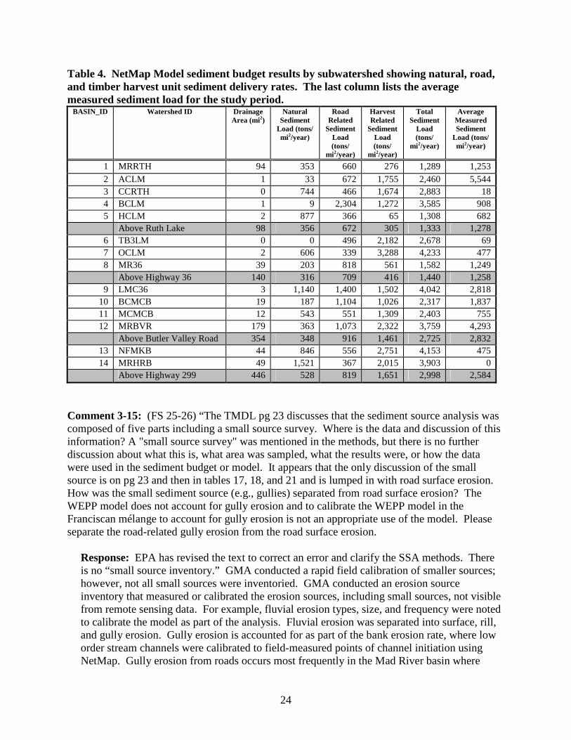
Table 4. NetMap Model sediment budget results by subwatershed showing natural, road, and timber harvest unit sediment delivery rates. The last column lists the average measured sediment load for the study period.

BASIN_ID Watershed ID Drainage Area (mi2)

Natural Sediment

Load (tons/ mi2/year)

Road Related

Sediment Load (tons/

mi2/year)

Harvest Related

Sediment Load (tons/

mi2/year)

Total Sediment

Load (tons/

mi2/year)

Average Measured Sediment

Load (tons/ mi2/year)

1 MRRTH 94 353 660 276 1,289 1,253 2 ACLM 1 33 672 1,755 2,460 5,544 3 CCRTH 0 744 466 1,674 2,883 18 4 BCLM 1 9 2,304 1,272 3,585 908 5 HCLM 2 877 366 65 1,308 682

Above Ruth Lake 98 356 672 305 1,333 1,278 6 TB3LM 0 0 496 2,182 2,678 69 7 OCLM 2 606 339 3,288 4,233 477 8 MR36 39 203 818 561 1,582 1,249

Above Highway 36 140 316 709 416 1,440 1,258 9 LMC36 3 1,140 1,400 1,502 4,042 2,818

10 BCMCB 19 187 1,104 1,026 2,317 1,837 11 MCMCB 12 543 551 1,309 2,403 755 12 MRBVR 179 363 1,073 2,322 3,759 4,293

Above Butler Valley Road 354 348 916 1,461 2,725 2,832 13 NFMKB 44 846 556 2,751 4,153 475 14 MRHRB 49 1,521 367 2,015 3,903 0

Above Highway 299 446 528 819 1,651 2,998 2,584

Comment 3-15: (FS 25-26) “The TMDL pg 23 discusses that the sediment source analysis was composed of five parts including a small source survey. Where is the data and discussion of this information? A "small source survey" was mentioned in the methods, but there is no further discussion about what this is, what area was sampled, what the results were, or how the data were used in the sediment budget or model. It appears that the only discussion of the small source is on pg 23 and then in tables 17, 18, and 21 and is lumped in with road surface erosion. How was the small sediment source (e.g., gullies) separated from road surface erosion? The WEPP model does not account for gully erosion and to calibrate the WEPP model in the Franciscan mélange to account for gully erosion is not an appropriate use of the model. Please separate the road-related gully erosion from the road surface erosion.

Response: EPA has revised the text to correct an error and clarify the SSA methods. There is no “small source inventory.” GMA conducted a rapid field calibration of smaller sources; however, not all small sources were inventoried. GMA conducted an erosion source inventory that measured or calibrated the erosion sources, including small sources, not visible from remote sensing data. For example, fluvial erosion types, size, and frequency were noted to calibrate the model as part of the analysis. Fluvial erosion was separated into surface, rill, and gully erosion. Gully erosion is accounted for as part of the bank erosion rate, where low order stream channels were calibrated to field-measured points of channel initiation using NetMap. Gully erosion from roads occurs most frequently in the Mad River basin where

24

roads dissect earthflow lithotopo units; this is accounted for as part of landslide sediment delivery. The TMDL document and the SSA (Appendix A to the TMDLs) were revised to reflect these differences; please see also Sediment Source Analysis Summary, above, and Appendix A to the TMDL document.

Comment 3-16: (FS 27-28) “We have reviewed the TMDL landslide source analysis and would like to provide better landslide and trend data for the Pilot Creek watershed. (See attachment C). We do not have a full landslide inventory however for the Upper Mad. The GMA report (table 27) states that a total of 1,320,819 tons of sediment were delivered in the Pilot Creek watershed (or 908 t/mi2/yr) over the past 30 years and 80% of the total is management related. The Forest Service data for Pilot Creek watershed (with a complete inventory of all landslides at the 1:16,000 scale) indicated that only 126,000 tons of sediment were delivered. This is an order of magnitude difference and substantial. In the North Fork Eel TMDL, landslide analysis using Forest Service methods was thoroughly scrutinized by independent contractors and determined to be valid and hence, was included in the North Fork Eel TMDL. The Pilot Creek landslide assessment was conducted by the same individual using the same methodologies. If the landslide data and protocol was sufficient for the North Fork Eel, we hope the same consideration can be used in the Mad River TMDL associated with the Pilot Creek watershed. Not only are the TMDL estimates of the amounts of sediment delivered from landslides within the Pilot Creek watershed significantly larger than the Forest Service estimates, but their association with management differs considerably. The GMA sediment source analysis indicates that 80% of the total landslide sediment sources are attributable to management activities. The Forest Service analysis indicates that the bulk of the landslides are inner gorge landslides, natural, and not management related (which is a considerable difference of data). This assessment covered 1944 to 1998. Between 1975-1990, the Forest Service found that in Pilot Creek, 51% of the landslides were attributable to harvest actives and none to roads. Out of the entire period of record (1944-1998), 92% of the landslides were natural and 8% were management related and the data indicate a steady and steep decline in management-related landslides. This data and analysis is present in attachment C and the GIS spatial coverage of this data will be provided to EPA.”

Response: The TMDL document and Appendix A to the TMDLs were revised to reflect the revisions to sediment source inputs; please see also Sediment Source Analysis Summary, above, and Appendix A to the TMDLs. Text has been added to the revised SSA to describe the results. GMA reviewed the Pilot Creek study for EPA referenced by the commentor (Dresser, 2003). The Pilot Creek analysis is conducted at a much smaller watershed, as the Pilot Creek subwatershed is an order of magnitude smaller than the Mad River basin (40 mi2, compared with nearly 500 mi2 for the Mad River SSA). Thus, the two are not directly comparable. Rather, GMA used the methods similar to those of DWR (1982), since the mapping scale and area were similar. This is appropriate for an analysis at this scale.

In general, EPA determined that the Pilot Creek study mapped landslides at a finer scale and split features more frequently than the SSA for the basin would allow. For example, the Pilot Creek landslide inventory broke out individual gullies within active earthflows, whereas this inventory lumped the gullies as larger earthflow features, then estimated a percentage of delivery. In addition, landslides smaller than five acres could not be accurately mapped for

25

the basinwide SSA, given the mapping resolution of the landslide inventory. EPA’s contractor (GMA) did not have access to most of the Pilot Creek subwatershed during field verification, due to ongoing logging operations on USFS lands, so field verification there was limited. However, where GMA did gain access, along the inner gorge of lower Pilot Creek, they found substantial differences between the USFS landslide data and conditions measured on the ground for several landslides. Also, the classification system is much different and not directly comparable. This is especially true for earthflow features. This could account for many of the differences between the two studies.

Nevertheless, EPA also reviewed one large landslide in the Pilot Creek subwatershed that was assumed to produce a relatively high sediment load. It was originally assigned to road-related causes but we determined that it should be assigned to natural causes because the feature had not increased in size as a result of the nearby road. This changed the sediment budget for the subwatershed significantly (see Table 1). However, it did not change the overall sediment budget significantly because the Pilot Creek subwatershed does not contribute substantial quantities of sediment to the basin.

EPA believes that GMA’s revised SSA reflects the best available information for setting the TMDLs. EPA encourages the Forest Service to provide more detailed data and information to the Regional Water Board, to assist in developing an implementation plan. The Regional Water Board may decide to develop TMDLs at the subwatershed scale, subject to EPA approval, and we would encourage the use of more detailed information at that scale.

Comment 3-17: (FS 29) “In the Upper Mad River, Anada Creek appears to be a large point source of sediment (see picture insets in GMA plate 12C). It is located in highly unstable geology and not representative of the rest of the upper Mad River basin. This is a small, un­roaded and un-managed watershed. In the TMDL, was this landslide attributed to natural or management related causes? We have looked at the photo record for this feature and it appears to be a natural feature. Likewise, the other landslide depicted in the plate 12C (bottom lower left picture) is a large natural grassland glade above Blue Slide Creek and not an earthflow feature as delineated in plate 12C and also has not changed for the photo record period (1944-1998). Please have this feature peer-reviewed and the data refined accordingly.”

Response: The Anada Creek slide, along with several other landslides within the South Fork Mountain Schist geology, occurs in the Upper Mad River subarea. Most of these landslides were field-verified as part of the landslide inventory. For the Anada Creek debris flow, several old roads and selective timber harvest units are located within and above the active crown of this feature. Several failed and diverting stream road crossings were mapped at the head of this landslide. In reviewing this information for EPA, GMA recognized that this is a naturally unstable hillslope, but concluded that road failure apparently has caused the crown to enlarge since the feature was initially mapped by DWR. The feature above Blue Slide Creek was mapped as active by DWR (1982), and appeared active on the 2003 aerial photographs. This feature was not field-verified by GMA; accordingly, it is coded as probable rather than definite.

26

While EPA does not peer-review TMDLs, we have re-evaluated the SSA data in response to these comments, and have made several revisions as described in Appendix A to the TMDL document. EPA feels that the data are sound for the scale that is undertaken, as described in the Sediment Source Analysis Summary, above. EPA encourages the Forest Service to work directly with the Regional Water Board to develop additional information for the implementation plan, and for revising the TMDLs in the future or to develop more detailed TMDLs on a subwatershed level, if the Regional Water Board determines that is appropriate, subject to EPA approval. The Regional Water Board may decide to peer review this information prior to developing an implementation plant; EPA supports such peer review.

Comment 3-18: (FS 30) “We are confused by the statement by GMA pg.2-15 that questionable landslides were not included in analysis unless field verified, yet the TMDL pg. 52 states that 11 percent were questionable and included. TMDL pg 52 also states that 56% were probable and only 33 percent were definite. The GMA report pg 4-6 statement that the confidence in the landslide assessment is medium to high when only 33% of landslides are definite seems overstated. Why is so much of the landslide data labeled probably or questionable? Should these be included in the TMDL?”

Response: Landslides that were classified as questionable and could not be identified as landslides during the field verification process were eliminated from further study, as stated in the TMDL document. The landslide inventory relied on the best available data and information for an assessment at the scale of the Mad River basin; this only allowed for limited field verification (i.e., 10-15%). In addition, access was limited during the field inventory, and several features originally selected to be field-verified could not be visited. The level of certainty in this analysis is appropriate for the scope of landslide mapping that was undertaken. Given the stated limitations and assumptions, the confidence is medium to high for this scale of inventory.

Comment 3-19: (FS 31) “Only 200 landslides were mapped for the entire Mad River watershed for the 1975-2003 period. In the Pilot Creek watershed alone, we mapped 394 landslides between 1944-1998. This clearly points to the differences in how landslides were mapped. Looking at the few air-photo insets in the color plates, it appears that the landslide interpretations were generous in their delineation of landslide areas (polygon boundaries) and included ground that the FS protocol would have considered stable (see Anada Creek inset). In addition, using aerial photos at the 1:24,000 scale is challenging to both identify and interpret landslides because the resolution is so poor. How many of the mapped landslides were completed using the 1:24,000 scale?”

Response: Most of the landslides were mapped at a 1:24,000 scale. The size of the Mad River watershed (nearly 500 mi2) limits the level of inventory possible, given the scope of the analysis. To map the entire Mad River basin at a more detailed scale is an enormous effort that could be undertaken in the future, if the TMDLs are revised, or during the implementation process. In addition, if the DWR pre-1975 active landslides are included in the total, then the results match the landslide frequency the USFS found. Detailed, on-the­ground erosion source inventories that can directly result in on-the-ground changes are

27

appropriate for the implementation effort. Regarding the Pilot Creek data, please see also response to Comment 3-16.

Comment 3-20: (FS 32) “Were the NAIP photos used in the air photo interpretation? NAIP photos are good to use for pictures but you cannot see them in stereo for accurate assessment of landslides. What percent of the landslide assessment was conducted using 2005 NAIP coverage?”

Response: The NAIP (National Agriculture Imagery Program) digital orthophotographs were used where more detailed aerial photograph coverage was not available. Available flight lines and years were limited on private lands. The Forest Service aerial photographs covered about two-thirds of the Mad River basin, and were used to verify the DWR (1982) landslide layer and map post-1975 active landslides. For most of the private land, the availability of aerial photographs was even more limited. As a result, GMA compiled all the available landslide maps from the DWR, CGS, and Green Diamond Resources, Inc. (2006). Additional mapping was completed in the field and from a low elevation flight. These data were used with the NAIP data to digitize active features in a GIS project. The features were mapped at a scale ranging from 1:15,000 to 1:24,000. Topographic relief was displayed using 10-meter DEM data. NetMap was then used to identify potentially active shallow landslide areas to include debris flows and earthflows, based on slope stability models (GEP). About 30 landslides were mapped from the low elevation flight and field inventory. These data and published landslide maps were used with NetMap to delineate active landslides.

Comment 3-21: (FS 33) “The TMDL pg 53 states that the majority of the mapped active landslides (81%) were debris flows yet in the next few sentences states that 56% of the landslides occur in the mélange and are mostly earthflows. Please clarify as these percentages don’t make sense”

Response: The commentor has pointed out a typographical error in the text: It should state that most landslides (81%) were earthflows, followed by debris flows. The text refers to the planar land area covered by features; earthflows occupy 81% of the planar land area of mapped active landslides (see also Table 14 in Appendix A). Sorting the planar land area of landslides by geology indicates that 56% of the planar land area occurs on Franciscan mélange geology; of these, most are earthflows, although earthflows also occur on other geology types (See Table 15 in Appendix A). Table 13 in the TMDL text (Table 16 in Appendix A to the TMDLs) also displays the count of landslide features. EPA regrets the error and has revised the text of the TMDLs to correct the error and clarify the differences in the descriptions. This error has also been corrected in the SSA.

Comment 3-22: (DS 34) “The statement in TMDL pg 57 that “ …unit deliveries range from 102 (Tompkins Creek) to 1194 tons/mi2/yr (North Fork Mad River). Landslides are typically not important sources in these subwatersheds.” This statement does not make sense nor does it match the data in Table 26, GMA. In every sediment budget conducted associated with TMDLs, landslides have always been the leading source of sediment. (refer to all published TMDLs) in the North Coast.”

28

Response: Within some subwatersheds (e.g., in the Upper Mad subarea), there were very few active landslides (Plate 12c). Naturally-occurring creep and bank erosion are the dominant background erosion sources, and surface erosion from roads is the dominant source of management caused erosion. In some subwatersheds, (e.g., Mud River and Deep Hollow Creek in the Lower Mad/North Fork subarea), there are also extensive and dense road networks. Relatively speaking, landslides are not typically important in subwatersheds with the highest and lowest rates of road-related surface erosion, although there are some exceptions. In addition, on a basinwide scale, landsliding rates are higher than surface erosion from roads.

Please note that the values of erosion sources have changed in most of the subwatersheds following revisions to the sediment budget; see Sediment Source Analysis Summary and Table 1, above, and the revised SSA (Appendix A to the TMDLs). Text has been changed in the TMDL document to reflect these changes and to clarify that while landslides are not important in some subwatersheds, they are generally the largest contributor of sediment in the basin as a whole.

Comment 3-23: (FS 35) “TMDL pg 60 states that “…Since WY 2006 was a very wet year and WY 2007 was very dry year, the suspended sediment loads were combined and averaged to produce a typical year.” The TMDL then used the average or “typical” year for comparing sediment loads among the reaches. It is not appropriate to take a flood year (2006) and a drought year (2007), average them and then say that the average represents a “typical” year. To take it to the extreme, we could take the 1964 flood year and the driest year of 1977(?) and call that “typical”. Refer also to comments from Bill Elliot (FS research – attachment A) who agrees that averaging these years is inappropriate, and not a good indication of an average value. Please develop a more scientifically robust method for developing average or typical sedimentation rates. This is critical given that these values are the baseline upon which the TMDL assesses background versus excess sediment.”

Response: The analysis uses best available data. EPA agrees that averaging the two water years may not produce an “average” year, but we believe that it does produce a reasonably typical year. In an effort to evaluate how close the SSA approach is to an average year, we modeled suspended sediment discharge over the 57-year period of streamflow records available at the USGS Mad River at Arcata gage. We used a Q vs. SSD (flow vs. suspended sediment delivery) relationship from the GMA 2006-2007 data (r2 = 0.93) and ran this through the mean daily discharges for the 57-year record. Using this method, the average of 2006 and 2007 loads was only 25% greater than the 57-year average (692,000 vs. 555,000 tons). These loads are not directly comparable to the loads computed in the SSA, since they were developed using different methods and 15-minute discharges. On the basis of this additional analysis, we feel that the average of the sediment discharges for two water years provides a reasonable approximation of a typical year. It is possible that the departure from average would be greater in the upper watershed, as the 2006 event was more unusual in that area than near Arcata.

Comment 3-24: (FS 36) “Ruth Reservoir: According to the TMDL (pg 72 Table 21), between 1975 and 2003, the Upper Mad River above the Ruth Dam has contributed 580 tons/mi2/yr of

29

which 67% is management-related. It is logical to think that the Ruth Dam would trap significant portions of this total load (as is acknowledged TMDL pg 55, pg 60, GMA pg 4-10) and a subset or smaller portion would be transported out of the system as suspended sediment. We contacted the Humboldt Bay Municipal Water District to determine what information they had regarding sedimentation rates behind the Ruth dam. Personal communication with Carol Rische (Humboldt Bay Municipal Water District staff) revealed that 10+ years ago they conducted cross sections behind the dam to determine the level of sedimentation infilling for maintenance purposes. Not only was the level of sedimentation behind the dam extremely low, but anecdotal evidence based on conversation with the District Engineer indicates that the tractor dozer marks associated with construction of the dam were still visible. Based on these findings, the Water District felt that frequent resurveying of the sediment levels behind the dam was not warranted due to the limited levels of sediment accumulation. The Water District is in the process of finding this staff report for use in this TMDL. She also stated that the bulk of the sediment entering the reservoir originates from Anada Creek and is associated with a natural landslide. She also stated that the bulk of the sediment sources are just above the reservoir and are easily spotted due to their sediment plumes and debris fans, which quickly settle out and does not appear to have reached the dam. She is available for further discussion. Please reconcile this information with the modeled data from the Draft TMDL.”

Response: The revised SSA has resulted in revised estimates in sediment production (see summary, above, and Tables 1-2, at the end of this document). Management-associated sediment is now estimated to comprise 38% of the total. However, this is at the MRRTH monitoring station, which does not include all of the sediment that enters Ruth Reservoir. EPA is confident that this estimate is the best that can be made of the sediment entering stream channels in the Upper Mad subarea. Not all of the estimated 234 tons/mi2/year is expected to infill the reservoir; a significant amount of the 199 tons/mi2/year that is estimated to make up the suspended sediment load probably bypasses the reservoir. Of the bedload and suspended load that does not pass beyond the dam, not all of it has yet reached the dam; much of it is stored in the low gradient alluvial reaches above the reservoir. Thus, our conclusions are not inconsistent with those of the HBMWD. EPA agrees that Anada Creek is the largest unit (i.e. per square mile) contributor of sediment (See Appendix A).

In addition, the USGS measured suspended sediment discharge at the Mad River near Forest Glen gage until the dam was closed. The average suspended sediment discharge between 1958 and 1970 was 108,400 tons/year or 758 tons/mi2/yr. It is unlikely that these sediment loads diminished immediately after construction of the dam. Thus, the sediment loads immediately prior to the dam closure were considerably higher than the revised SSA loads. As noted above, much of the coarse load is stored in the high flow backwater area of the reservoir and just upstream, and may not have been evident in the cross sections surveyed. Evaluating reservoir deposition is a challenging endeavor, and accurate results require complete bathymetry rather than cross sections. Accuracy depends heavily on the quality of the original topography, which is often the limiting factor. Suspended sediment loads at MRRTH measured in 2006-2007 for the SSA were 2,479 and 27 tons/mi2 for the two water years, respectively, considerably higher than the 1958-1970 data or the sediment budget portion of the SSA. It is doubtful that loads such as 2006 would not be detectable in a comprehensive reservoir sedimentation survey.

30

Comment 3-25: (FS 37) “Hetten and Tompkin Paired Watershed Study: This paper studies the effects of timber harvest treatments with Best Management Practices on water quality. Suspended sediment concentration, discharge and turbidity were measured from 1985-1993. Reference conditions were established and compared to post- treatment conditions. No management-related increases in SSC or turbidity with discharge were found. That is, under current management, sediment discharge from Forest Service lands is already within the range of natural variability, much less 20% over background. Also, since 1994 the Six Rivers has been operating under the Northwest Forest Plan. The Northwest Forest plan is more restrictive in terms of harvesting adjacent to or within riparian reserves and unstable areas as compared to the timber practices that were implemented during this study. A copy of the Master Thesis has been sent to you. Please reconcile this study with the modeled data from the Draft TMDL.”

Response: EPA disagrees with the commentor’s conclusions about the results of the Hetten and Tompkin Creeks paired watershed study (Barber, 1997). In fact, we believe this study indicates that increases in suspended sediment concentration (SSC) and turbidity can be expected following timber harvest treatments, even with Best Management Practices. This is also found in other studies; for example, Klein (2003, 2006) concluded that increased turbidity is associated with timber harvest practices, although he did not specifically investigate whether and how BMPs were employed. In the Hetten and Tompkin paired watershed study (Barber, 1997), four different methods were used to investigate the relationships between suspended sediment concentration (SSC), discharge, and turbidity. For two of the techniques (Sediment Yield and Cleansing Storm), the author “concluded that there was a statistically significant increase in suspended sediment concentration and turbidity as a result of watershed treatment” (pg. 162). The other two techniques (Standardizing Sediment Yield by Storm Water Yield and the Hysteresis technique) did not identify any increase that could be attributed to the watershed treatment.

In addition, our reading of the report led us to believe that the methods were flawed. For example: 1. The author clearly states that “ ‘reference conditions’ monitored included the effect of

some road building” in both the control and reference watersheds prior to treatment (pg. 153). The author goes on to state that the road building biased the reference conditions established and that the probable result is that SSC and turbidity for any given flow was overestimated, thereby reducing the detectability of any treatment related effects (pg. 154).

2. No data are available for the largest storm of the study period, and it appears from the text that the data for the second largest flow event was not adequate and was therefore not used in the analysis (pg 35-36). It is a generally accepted theory that the majority of sediment is transported during a very short interval during large peak events.

3. The author recognizes that the sampling scheme was sensitive to “Cleansing Storms” and that often, early storms were missed and may not be adequately represented.

4. The study occurred during a relatively dry period when compared to the 20-year average. The post-treatment period was drier than the pre-treatment period (pg.75). Thus, the data could be more influenced by climate conditions than by treatment.

5. All post-treatment turbidity samples collected on cleansing storms in the treatment watershed exceeded 20% over background (pg 123). The author acknowledges that as

31

flows get higher there is not a discernable difference between pre-treatment and post­treatment. This could be the case, but could also be an artifact of the large variation in samples taken at higher flows. Discharge, while correlated with SSC and turbidity during this study, was not highly correlated, and therefore introduced a large amount of uncertainty. A study using turbidity as a surrogate for SSC would likely eliminate a large portion of this uncertainty and would be able to better answer the question as to whether post-treatment changes were detectable.

Comment 3-26: (FS 38) “Although clear that GMA did a good job measuring SS and turbidity, it is not clear how this data was incorporated into the final sediment budget. The TMDL (section 3.1.2.6) states that bedload was assumed to be from 5-15% of total sediment load, so was the measured SS value used to estimate tons of bedload? How was this used in relation to other input values like the tons of sediment from landslides?”

Response: The measured sediment data were not directly incorporated in the sediment budget. The measured load values were used to inform the NetMap model, but the results of the NetMap sediment budget are not included in the traditional sediment budget, from which the TMDL is set. Bedload is commonly found to be 4-5% of total load for large, low-gradient alluvial rivers, and 10-25% for steeper, smaller channels (Collins and Dunne 1990, Reid and Dunne 1996, Lehre 1993). Please see also Sediment Source Analysis Summary, above.

Comment 3-27: (FS 39) “There is a very confusing statement in GMA page 2-20. “For modeling purposes, the measured load at the basin outlet was estimated to be 25% of the existing load.” Are you taking actual measured data and adjusting it to fit your model? If you are measuring sediment output, it seems like this would be an extremely valuable part of the sediment budget.”

Response: Upland erosion, sediment delivery, and sediment load were estimated and used to scale the GEP portion of the NetMap model (see Sediment Budget Summary, above, and Appendix A to the TMDL document). Sediment yield and sediment load were developed using actual measured data. The Generic Erosion Potential (GEP) factor was scaled to average basin sediment load (the basin average sediment load divided by the basin average GEP was applied as a conversion factor: units of GEP to units of sediment load). The approach is similar to a design storm analysis, and the loads were chosen to help proportion the sediment load realized at the basin outlet amongst the upland lithotopo units. The goal was to identify the large erosion hazards that are realized in the sediment load near the mouth of the Mad River.

Comment 3-28: (FS 40) “In (GMA p.3-62) a Severity of Ill Effects scale is presented. At the mouth, turbidity/SS levels are more or less always sublethal to lethal. At Ruth Reservoir (MRRTH) the maximum recorded value is "sublethal". The 50% exceedence is "behavioral" and 90% is basically no effect ("alarm reaction"). The highest measured value at MRRTH is near the recovery level at Blue Lake. Is this is the same storm that produced 63% of total measured load (over the two year period), 223 mg/l? Again, if over a two year period, 63% of the sediment came in one event that lasted a few days, is it clear that this watershed is impaired?”

32

Response: The Severity of Ill Effects (SEV) scale devised by Newcombe and Jensen (1996) is not related to sediment loads in individual storms; rather, it is related entirely to duration of exposure to elevated suspended sediment and turbidity. Individual storms are considered within the context of total flow over the period of monitoring to estimate a percent exceedence and duration. Thus, according to the SEV scale, the site is indicated as impaired because of the duration and severity of exposure, not the peak suspended sediment concentration or load. However, it is important to note that the SEV scale did not appear to fit circumstances at the Mad River basin, and was not used to set the TMDLs. In fact, applying that scale to durations of exposure derived from the turbidity exceedence values developed by GMA (Appendix A to the TMDL) using Klein (2006; unpublished data, 2007) suggested that undisturbed streams would be categorized as SEV 4 or 5 (significant behavioral effects to sublethal effects). Moreover, correlations reported by Newcombe and Jensen (1996) were weak. For this reason, the discussion is provided as another source of information on turbidity, but the information is not used substantively.

Comment 3-29: (FS 41) “Load reductions associated with management activities were set between 90 to 98% (TMDL, Table 21 pg 70). Every land manager has the legal responsibility to reduce their sedimentation rates, but setting the target reductions to 90 or 98% is not practical in this geology. Setting such high values would indicate that the goal is to completely reduce all anthropogenic presence within the watershed. Undoubtedly some proportion of the total roads could conceivably be removed or decommissioned, but there will always be key access roads that will remain in place. Many of these key access roads that bisect unstable geologies will remain in place and there should be acknowledgement in the TMDL that a 90-98% reduction is desirable but not truly achievable (see also comments from Bill Elliot – attachment A). Without acknowledgement of these facts, the TMDL leaves land managers wide open to legal challenges.”

Response: The Regional Water Board has the authority to set water quality standards, and TMDLs developed by either the Regional Water Board or EPA must be set at levels necessary to meet those water quality standards. Our analysis indicated that the watershed is highly impaired; much of the sediment and turbidity is related to management, and this analysis is also supported by information showing that impairment in the watershed is linked to declines in the cold freshwater beneficial use. Unless the water quality standards are changed, or site-specific standards are developed by the Regional Water Board, it may be that removing roads in unstable geologies is necessary to achieve the water quality standards. Please see also Sediment Source Analysis Summary, above, and Tables 1-3 for information about changes resulting from the revised SSA.

Comment 3-30: (FS 42) “If at all possible, we would like to see the load allocations broken down by large landownership, particularly in the Middle Mad River watershed. It is important to separate the Forest Service contributions from those of other large land managers. Such an effort will make it readily apparent to the public what contributions are from the Forest Service in light of the larger sedimentation issues within the Mad River watershed.”

Response: The Regional Water Board has authority to develop revised TMDLs, subject to EPA approval, on a subwatershed basis. The Regional Water Board also has authority to

33

develop implementation plans for the TMDLs established by EPA, and may utilize information from the Forest Service in order to work on an ownership basis. EPA encourages cooperation with the Regional Water Board in refining the information used to develop and implement TMDLs. Although EPA does not plan to further develop individual subwatershed­scale TMDLs at this time, we encourage the Regional Water Board to consider doing so, and we encourage the Forest Service to work cooperatively with the Regional Water Board in order to ensure that the best available information is used.

Comment 3-31: (Bill Elliot) “The first concern is that the report tends to want to focus on "average" erosion and sediment delivery rates. This is not good science. Erosion and sediment delivery are episodic in nature, and disturbance driven. The report did not reflect that. The report suggested that the average of a wet year and a dry year were a good indication of an average value. This is unlikely. If the wet year was the wettest in five years, then the average value is more likely the average of one wet year and four dry years. The degree of wetness of their wet year for setting sediment delivery needs to be determined before deciding what is "average".”

Response: TMDLs are described under Section 303(d) of the Clean Water Act as the maximum daily load that the waterbody can receive and still meet water quality standards. EPA recognizes long-term sediment loads are driven by episodic flood events. For this reason, the TMDLs are described as average annual loads, based on 15-year or longer averages. Please see also response to Comment 3-23.

Comment 3-32: (Bill Elliot) “One episodic event in particular that is a major source of sediment in forested watersheds is wildfire. This was not considered in the analysis. In the absence of considering sediment from wildfire, the entire analysis does not adequately address the background erosion rates. Many forest watersheds have wildfire every 50 to 200 years, and then spend decades routing the sediment from the wildfire through the stream system, generally in years with above average precipitation only.”

Response: No large fires have occurred within the Mad River in the last 5-10 years. Even though wildfire is not included specifically as a category in the sediment budget, it is considered incidentally. For example, sediment related to salvage harvest following a wildfire is captured due to the effect from the road system. However, it is difficult to predict the effects from wildfire, which are relatively small (and sporadic) at this scale, particularly considering that the Mad River basin occupies two (or more) very different climatic zones: coastal and inland. Wildfire is not a factor that is driving the overall sediment budget. Please see also response to Comments 3-4 and 3-11.

Comment 3-33: (Bill Elliot) “The road erosion predictions are problematic. From Appendix 2 in the Sediment Source Document, it appears that all roads were considered as High traffic. This is highly unlikely. Low traffic roads will only generate about a fourth (or less) of the sediment as a high traffic roads. I suspect that less than a fourth of the forest roads in this drainage would be classified as having high traffic.”

Response: EPA agrees that the original estimates of road-related surface erosion were high. Please note that the proportions of sediment inputs from various sources and subwatersheds

34

have changed following revision to the SSA. Changes to assumptions in the WEPP model were developed in coordination with the commentor, who was the co-developer of the model. Please see Sediment Source Analysis Summary, above, and the revised SSA (Appendix A to the TMDL document).

Comment 3-34: (Bill Elliot) “All streamside roads were modeled as having a gradient of 10 percent. This is unlikely, in that generally, streamside roads have a gradient similar to the stream, which is often less than 1 percent. This gross over prediction of roads along streams, coupled with the minimal buffer distance assumed results in a gross over prediction of streamside road erosion. I would want to see some data about the gradient of streamside roads before accepting the reports conclusions about the extraordinarily high road erosion predictions.”

Response: Please note that the proportions of sediment inputs from various sources and subwatersheds have changed following revision to the SSA. Changes to assumptions in the WEPP model were developed in coordination with the commenter, who was co-developer of the model. Please see Sediment Source Analysis Summary (above) and the revised SSA (Appendix A to the TMDLs).

Commentor 4: Michael Long, United States Fish and Wildlife Service

Comment 4-1: “The Services listed species are not addressed in the document. We are concerned that future planning efforts and potential development of implementation plans based on this draft TMDL document may not adequate consider impacts to our species. More specifically we are concerned with potential effects to the threatened western snowy plover (Charadrius alexandrinus nivosus). The lower Mad gravel bars may be important snowy plover nesting sites. Since most of the draft TMDL’s analysis, suggested allocations and targets are based on habitat requirements for salmonids, they do not address the habitat requirements for the snowy plover. Attainment of most of the presented targets will not effect, or may also be beneficial for our species habitat requirements. However, some activities, like gravel bar removal, and estuarine habitat modification under taken as to meet some of the TMDL targets may impact them.

Response: EPA agrees that attainment of the TMDL should not adversely affect these species. With regard to the concerns regarding implementation of the TMDL, EPA has added language recommending that agencies undertaking any activities that could affect those species, either for TMDL implementation or other activities, consider the unique habitat needs of the western snowy plover, and to consult with FWS as appropriate. Text has been added to Chapter 2 and Chapter 4 to identify and describe the western snowy plover, and to Chapter 4 to highlight additional concerns that should be addressed when developing implementation plans. The western snowy plover is threatened by human disturbance, including recreation, predation, and loss of nesting habitat to non-native species and urban development (USFWS, 2007, http://www.fws.gov/arcata/es/birds/WSP/plover.html). Reducing sediment and returning to conditions more reflective of natural temperatures are not expected to adversely affect the species, but, in response to this comment, EPA has added text regarding actions (not necessarily related to TMDL implementation) that could affect the species.

35

Comment 4-2: “We suggest that you include some general language that mentions the occurrence of the snowy plovers in the TMDL project area. In addition, under Chapter 5, state that some activities undertaken to meet the suggested TMDL targets, such as removal of gravel for the Mad River gravel bars may affect snowy plover nesting habitat. ESA Section 7 consultation with the Service will be required for activities that may affect our species.”

Response: Text was added to Chapter 2 and Chapter 4 to address these concerns. See also response to Comment 4-1.

Commentor 5: Tharon O’Dell, Green Diamond Resource Company Ed Voice and Family, Interested Party

Comment 5-1: “A thirty-day comment period does not provide a meaningful opportunity to review and comment on this highly technical document. Accordingly, Green Diamond hereby requests a 30-day extension of the comment period for this TMDL… Green Diamond is a major landowner in the Mad River watershed whose interests may be significantly affected by the draft TMDL. In addition, Greene Diamond’s subsidiary California Redwood Company operates a manufacturing facility in the Mad River watershed and holds an NPDES permit for discharges within the watershed. Green Diamond cooperated with EPA’s TMDL contractor, Graham Matthews and Associates (GMA), by providing information to GMA under a Data Use Agreement. In exchange for Green Diamond’s cooperation, GMA promised to Green Diamond a meaningful opportunity to review and respond to the work done by GMA prior to its release by EPA. GMA did not provide Green Diamond with the requisite opportunity… U.S. Fish and Wildlife Service and the National Marine Fisheries Service have provided the interested public with 60-day review and comment periods for highly technical projects proposed by Green Diamond.”

Response: EPA appreciates Green Diamond’s efforts to assist with the development of the TMDLs by providing data to GMA. EPA regrets that we are unable to grant Green Diamond’s request to extend the comment period due to our schedule obligations under the Consent Decree, which requires that the TMDLs be finalized, including consideration of public comments, in 2007. Also please see response to comment 5-2.

Comment 5-2: “In Chapter 4, p. 79 paragraph 2 of the draft Mad River TMDL, the EPA has appropriately acknowledged that more reliable information on sediment and turbidity should be used to refine the TMDL… Green Diamond agrees that the methods and information provided in the TMDL are too coarse and likely in error. It is therefore imperative that EPA and the Regional Water Board approach the implementation of the TMDL with caution and flexibility recognizing that there is higher quality, site-specific information on sediment conditions and sediment management in the Mad River Basin. Green Diamond welcomes the opportunity to provide the opportunity to provide the Regional Water Board with such information.”

Response: EPA encourages Green Diamond’s participation in implementation efforts with the Regional Water Board. More detailed information at a subwatershed scale can facilitate effective implementation of the TMDLs, as well as the potential for development of

36

subwatershed-scale TMDLs by the Regional Water Board and others, as appropriate, and subject to approval by EPA. Please note that the proportions of sediment inputs from various sources and subwatersheds have changed following revision to the SSA. Changes to assumptions in the WEPP model were developed in coordination with Bill Elliot, co­developer of the model. Please see Sediment Source Analysis Summary and Appendix A to the TMDL document.

Comment 5-3: “The draft Mad River TMDL did not reference or consider existing detailed scientific information concerning sediment management in the Mad River Basin that is found in the Green Diamond Resource Company Aquatic Habitat Conservation Plan and Candidate Conservation Agreement with Assurances (October 2006) and the Final Environmental Impact Statement for the AHCP (October 2006). The draft TMDL utilizes an across-the-board allocation of sediment load to land management types (i.e., management-related road sediment) that is inappropriate given the detailed and enforceable sediment reduction commitments in the AHCP, which EPA did not consider.”

Response: Green Diamond’s HCP and EIS, both the text and the appendices, were reviewed and utilized by EPA’s contractor (GMA) in the revision to the SSA. Please note that the proportions of sediment inputs from various sources and subwatersheds have changed following revision to the SSA. Changes to assumptions in the WEPP model were developed in coordination with Bill Elliot, co-developer of the model. Please see Sediment Source Analysis Summary (above) and the revised SSA (Appendix A to the TMDLs). EPA appreciates that the documents were made available, and acknowledges Green Diamond’s cooperative efforts to provide data and allow access to its lands.

Comment 5-4: “EPA has not completed consultation with the National Marine Fisheries Service under Section 7 of the Endangered Species Act prior to proposing the draft TMDL for adoption. This section 7 consultation should be completed so that EPA has the benefit of NMFS’ expertise on sediment management issues and listed species effects in the Mad River Basin. A completed consultation likely would also provide EPA with a better opportunity to consider the sediment management commitments of the AHCP, which were developed in cooperation with NMFS and approved by NMFS.”

Response: EPA acknowledges that its consultation with NMFS and FWS are not yet complete. EPA believes it is unlikely that the Services will conclude that the TMDLs that EPA is establishing violate Section (7)(a)(2) of the Endangered Species Act, since the TMDLs and allocations are calculated in order to meet water quality standards, and water quality standards are expressly designed to “protect the public health or welfare, enhance the quality of water and serve the purposes” of the Clean Water Act, which are “to restore and maintain the physical, chemical, and biological integrity of the Nation’s water.” Additionally, this action will improve existing conditions. However, EPA retains the discretion to revise this action if the consultation identifies deficiencies in the TMDLs or allocations.

Comment 5-5: “Although assumptions are listed with certain elements of the sediment source analyses, a number of the assumptions used to develop rates, volumes or management associations are employed without supporting reference or explanation. It then becomes

37

impossible to understand why things were done the way they were or why certain methods or assumptions were used in the analysis. For example, why is 35% used as the demarcation of “steep slopes” for mass wasting processes (Table 4) when this is not supported in the literature? Why are all landslides located within 100 feet of a road assigned a “road-related” causal factor? Why are all slides classified as a certain type (e.g., debris slides) assigned a single depth when calculating slide volumes, regardless of their aerial size (Table 3)? These “assumptions” or procedures have the potential to dramatically affect sediment delivery volumes and causal associations (natural versus anthropogenic) in the analysis, yet their use is not explained or referenced as being commonly employed in the development of sediment budgets.”

Response: EPA acknowledges a typographical error in Table 4 of the SSA. The categories should read as follows:

Inner Gorge (>65%) Steep Slope (35%-65%) Gentle Slope (<35%) Ridgeline

The text of the SSA was changed to correct this error.

Please note that the proportions of sediment inputs from various sources and subwatersheds have changed following revision to the SSA. Changes to assumptions in the WEPP model were developed in coordination with Bill Elliot, co-developer of the model. Please see Sediment Source Analysis Summary (above) and Appendix A to the TMDL. One of those changes was to change the automatic assignment of road-related causes to any landslide within 100 ft of a road. Instead, landslides are assigned road-related causes if they cross a landslide. This change in classification affected six slide features; the available data were reviewed to ensure that the slides did not appear to be causally related to the roads, which were within 100 ft but were not crossing the features.

Comment 5-6: “Why is a single landslide depth employed for calculating landslide volumes from each landslide type regardless of the size of the landslide? For example, a debris slide that is 200’ x 100’ is assumed to have a depth of 9 feet (Table 3). Similarly, a large inner gorge landslide that is 200’ x 500’ is also assumed to have the same 9 foot average depth. This assumption will lead to skewed landslide delivery rates. For example, very large inner gorge landslides along the main stem of the Mad River and its largest tributaries are most likely to be natural, and this nine foot assumed average depth (Table 3 is likely to lead to a significant underestimate of landslide volumes for these largest landslides. Similarly, using a set of landslide depth of nine feet is equally expected to overestimate the contribution of the smaller management-related debris landslides. This “one-depth” assumption will seriously skew the sediment delivery data relative to causal factors. A more acceptable methodology would have been to develop a regression equation between landslide dimensions (e.g., area) versus mean landslide depth from the sample of field-checked landslides, and then to apply this relationship to landslides mapped in the air photo analysis. The depth-based regression provides A statistically robust method for deriving depth for each erosion feature. This is a common practice in the science and has been used in TMDL studies and watershed analysis elsewhere.”

38

Response: EPA agrees that the area/depth relationships overestimated the contributions from small landslides, and underestimated the contributions from large landslides. Please note that the proportions of sediment inputs from various sources and subwatersheds have changed following revision to the SSA. Changes to assumptions in the WEPP model were developed in coordination with Bill Elliot, co-developer of the model. Please see Sediment Source Analysis Summary and Appendix A to the TMDL document. As part of this revision, the depth/volume relationships were reexamined, and, although a good correlation was obtained, it was determined that the new results were so high that they would have reflected rates in highly active areas of New Zealand and diverged significantly from rates in the California North Coast. Accordingly, the rates were adjusted according to the Washington State Manual for Conducting Watershed Analyses (WA DNR, 1995). See Sediment Source Analysis Summary, Landslide Analysis section.

Comment 5-7: “GMA chose to assign one average rate of sediment delivery for each of 12 landslide types (Table 4). The assumptions, data or references used to derive the delivery coefficients in this table are not stated and there is no way to check the appropriateness of the assumed values. It is important to note that sediment delivery within each of the 12 landslide categories can be highly variable. Sediment delivery is best evaluated from analyzing the aerial photos, visually estimating sediment delivery and then checking the delivery estimates during the field surveys. If the data set is large, the field survey can be used to develop relationships and “adjust” the yields that were estimated from the air photo analysis. However, the very small data set of field-checked landslides (only 31 field-verified landslides in all) in the Mad River TMDL analysis would not allow meaningful relationships to be developed for all 12 landslide types listed in Table 12. Unfortunately, the delivery coefficients used in this table have a profound effect on the final sediment delivery volumes that are presented in the sediment budget tables. For example, small changes in the “assumed” delivery coefficients (Table 4) for the four earthflow categories will make a disproportionately large impact on total landslide inputs and on the total landslide sediment delivery that is assigned to the background or natural category.”

Response: Please note that the proportions of sediment inputs from various sources and subwatersheds have changed following revision to the SSA. Changes to assumptions in the area/depth were made as part of these revisions (see response to Comment 5-6). Each of the 12 landslide types was assigned one of four delivery coefficients based on hillslope position, slope steepness, and proximity to an active stream channel. In the case of earthflows, the delivery coefficient was manually adjusted to match the sediment delivery rates measured in the field and from remote sensing data where sediment delivery occurs near the toe and within lateral gullies dissecting the features.

Comment 5-8: “In the GMA report all landslides located within 100 feet of a road are assumed to be road-related/management-caused (Appendix A, 2.4.1.7). This assumption may or may not be generally valid or appropriate, but its use has not been supported with field data from the Mad River watershed or by other reference in the scientific literature. In fact recent studies performed in the near by Redwood Creek watershed by California’s North Coast Watershed Assessment Program (Falls, J., McGuire, D., and Dell’Osso, D., 2003) indicate that there is a strong correlation between roads and landslide incident between 0 and 75 feet but virtually no correlation beyond 75 feet.”

39

Response: Please see response to Comment 5-5. This assumption was revised in the revised SSA.

Comment 5-9: “Landslides on post-1975 harvest areas (i.e., all slides <30 year old) are assumed to be management-caused (Appendix A, 2.4.1.7). No explanation as to the source of this assumption was provided, leading the reader to assume that naturally occurring landslides cease to exist in those areas. In addition, other non-management causal factors often come into play and these are not evaluated or accounted for in the GMA attribution protocol. For example, very large inner gorge landslides along the main stem Mad River and in major tributaries may, in many cases, be cause by channel migration and undercutting. These large volume slides would have been arbitrarily assigned a management association even though their geomorphic setting might clearly indicate they were triggered by natural channel migration processes. In addition the use of the 2003/2005 aerial photo set limits this cause and effect assumption in that recent landslides observed on these photos may be attributed to timber harvesting that occurred 20 to 30 years prior. In general correlation between timber harvesting and landslide incident is not thought to be strong beyond 20 years of re-growth. The use of a one-size-fits-all causal classification, without the mechanism to professionally review and reassign causal associations is likely to lead to significant misclassifications of mass wasting features. When it comes to the largest of the basin’s landslides (those along the inner gorges) this can also skew the data away from natural causes and towards management-related sediment delivery.”

Response: EPA acknowledges that there is some uncertainty in the SSA. We also acknowledge that most slope failures probably occur between 7 to 10 years following timber harvest or wildland fire, and that some errors may have occurred in assigning landslides to timber harvest causes. However, we feel reasonably confident that we have adequately made these assignments. Timber harvest activities (other than those associated with roads) are not the driving forces in sediment production in the watershed. In fact, the landsliding rate assigned to timber harvest causes is estimated to be extremely low (38 tons/mi2/year). This unit rate has decreased from the rate estimated in the draft SSA, primarily due to changes in the assumptions regarding landsliding depth. Please note that the proportions of sediment inputs from various sources and subwatersheds have changed following revision to the SSA. Please see Sediment Source Analysis Summary and Appendix A to the TMDL document.

Comment 5-10: “Slope steepness is an essential contributing factor to mass wasting occurrence and downslope transport of landslide materials (sediment delivery). In the GMA mass wasting analysis “steep” slopes have been assigned a value of >35% (Table 4). No information has been provided as to the significance of a >35% slope class in mass wasting, nor has its relevance been referenced from the literature. Typically, slope breaks of 50% and 60-65% are used in the designation of slopes susceptible to mass wasting. Slopes in the 35% class range are typically stable, unless they occur in combination with earthflows or other types of flows.”

Response: EPA’s contractor (GMA) used the following slope breaks: Ridgetop (flat); Gentle (<35%), Steep (35%-65%); and Canyon Bottom (>65%). The typographical error has been corrected. Please see response to Comment 5-5.

40

Comment 5-11: “Several tables in the back of the GMA report, as well as several tables in the EPA TMDL document (e.g., PEA Table 17), contain data for sediment delivery from streambank erosion processes. However, there is no GMA methods section for the measurement and analysis of bank erosion nor is there a discussion of the results of the bank erosion study. Typically, a field sample of bank erosion measurements is collected along a representative set of stream channels and the data is then extrapolated to the rest of the drainage network. Air photo analysis of bank erosion is used only along major channels to mark zones of channel migration and major shifts of low gradient stream reaches. Without the methods section and the data, this important component of the sediment budget cannot be evaluated.”

Response: The methods section has been expanded in the revised SSA to describe the data collection for streambank erosion processes. Please see Sediment Source Analysis Summary, above, and Appendix A to the TMDLs.

Comment 5-12: “We believe [landslides] ‘have been significantly underestimated in their volumetric importance.’” The rationale for using the 1975 and 2003/2005 aerial photo periods “is not stated, and therefore the reader must assume GMA is suggesting that all post-1975 landslides important to the sediment budget process will be visible from the 2003/2005 photo set. This is highly unlikely and the assumption that all the landslides during this 30 year period were observed and documented from the 2003-2005 photo set has likely led to a gross underestimate of landslide sediment contributions in the sediment budget. Mass wasting analyses completed for projects elsewhere, including other north coast TMDL sediment studies and watershed analyses, have typically employed air photo sets that are selected to bracket major landslide-producing storms, and at a minimum one set is analyzed for each decade of analysis. This helps ensure that landslides that occur in one decade will be observed before their scars revegetate and are no longer visible.” The landslides are significantly underestimated because only one photoperiod is used.

Response: Please see responses to Comments 5-6 and 5-7 regarding the analysis of the depth/area relationships for slides, as well as the response to Comment 3-16 regarding various scales of studies. EPA feels that the results of the analysis are appropriate to the scale of the study, and utilize the best available data. Please note that the proportions of sediment inputs from various sources and subwatersheds have changed following revision to the SSA. Please see Sediment Source Analysis Summary (above) and Appendix A to the TMDLs

Comment 5-13: “The GMA report does not reference the importance of the extensive occurrence of earthflows in the watershed as they relate to fluvial erosion, suspended sediment and turbidity. Much of the sediment that originates from deep-seated landslides and earthflows within terrain that is known to be highly erodible (i.e. Franciscan Melange) actually comes from shallow failures, gullying and surface erosion processes (Kelsey 1977, 1978). These natural sediment delivery processes are even at work on large deep seated slides and earthflows that are classified as “stable” and not currently active or moving. This source … is not accounted for in the GMA analysis. Earthflow erosion and sediment delivery for the 31 year time period should not be based on the entire earthflow area, an average 12-foot depth, and an average 5% earthflow sediment delivery. Earthflow erosion … should reflect gully erosion of the slide surface and earthflow toe erosion. The GMA air photo analysis did not identify any gully erosion features,

41

although they do comment on the prevalence of gullies in the Franciscan Melange…. Gully erosion accounted for 5.5% of the total sediment budget in Redwood Creek. In addition, earthflow movement is typically activated after high annual precipitation years, and as a result erosion and sediment delivery occurs at the toe of the active earthflows through stream undercutting.” Earthflow retreat (+ (movement) rates have been developed for past TMDL studies in the Middle Main Eel River, Lower Eel River, and Freshwater Creek.”

Response: The revised SSA contains additional information regarding how earthflows were accounted for in the analysis. Please note that the proportions of sediment inputs from various sources and subwatersheds have changed following revision to the SSA. Changes to assumptions in the WEPP model were developed in coordination with Bill Elliot, co­developer of the model. Please see Sediment Source Analysis Summary (above) and Appendix A to the TMDLs. Appendix A to the draft TMDLs, and the draft TMDL document itself, contained a typographical error that may have mislead readers about the importance of earthflows; this has been corrected. Please see also response to Comment 5-21.

Comment 5-14: The GMA analysis of sediment delivery from earthflows is weak, especially related to activity level, rates of movement and sediment discharge. Earthflows are assumed to deliver 5% of the displaced volumes… Nowhere in the analysis are there any supported assumptions about earthflow movement rates, erosion processes and sediment delivery, either from direct observation, air photo analysis or from the literature. There is no way the resulting yield data from these deep-seated mass wasting features can be evaluated or confirmed. In an analysis of a number of TMDL sediment studies, CGS (2002) similarly concluded that there was an underestimation of natural landslides movement and sediment production from large landslides and from gully erosion processes on both active and dormant deep-seated landslides.”

Response: The revised SSA contains additional information regarding how earthflows were accounted for in the analysis. Please note that the proportions of sediment inputs from various sources and subwatersheds have changed following revision to the SSA. Please see Sediment Source Analysis Summary above and Appendix A to the TMDLs.

Comment 5-15: “The air photo analysis of past sediment sources only included features greater than 3000-5000 ft2. The analysis does not provide any information about inputs from smaller sediment sources such as landslides and bank erosion. Although the GMA report states that GMA staff mapped smaller landslides in the limited field sampling (pg 2-11), there is no mention of how this data was used to understand the gap in information for inputs from smaller sediment sources. Past studies in nearby watersheds (Upper Eel River Watershed Analysis, PALCO 2007) have shown that the small streamside landslides and bank erosion features can increase total watershed-wide sediment delivery by up to 50%, depending on the drainage density. Many of these smaller erosion features are obscured by vegetation and cannot be readily identified at the scale of the aerial photography. Other studies have incorporated smaller sediment sources into the sediment budget by conducting streamside landslide and bank erosion inventories along stratified sample reaches by Strahler stream order, and then extrapolating derived rates for landslides and bank erosion to the entire stream system. This important component of the Mad River watershed sediment budget is missing.”

42

Response: Please see responses to Comments 5-6 and 5-7 regarding the analysis of the depth/area relationships for slides, as well as the response to Comment 3-16 regarding various scales of studies. EPA feels that the results of the analysis are appropriate to the scale of the study, and utilize the best available data. Please note that the proportions of sediment inputs from various sources and subwatersheds have changed following revision to the SSA. Please see Sediment Source Analysis Summary (above) and Appendix A to the TMDLs. Please see also response to Comment 3-16.

Comment 5-16: “The GMA report does not reference the importance of seismicity. The Mad River is located in a tectonically active area known as the Mendocino Triple Junction (MTJ). Within the MTJ and the Mad River watershed is the highly active Mad River shear zone, which encompasses 4 known active faults. It is well known that historic earthquakes in the area have resulted in elevated landslide incident (Youd and Hoose, 1978; McPherson and Dengler, 1992) and as a result elevated sediment delivery. None of this was discussed by GMA and therefore it is assumed that this was not taken into consideration.”

Response: Earthquake activity, including the April 1992 seismic events, could predispose potentially unstable areas to the risk of landslide failure, and likely caused localized changes on a scale not addressed by this analysis. Large earthquake events can disrupt or redistribute slope waterpore pressures, and can affect landslides. In performing the SSA, GMA did not investigate earthquakes or seismicity as a measurable triggering mechanism. Given the uncertainty of seismic events, it is difficult to assign a seismic triggering mechanism (Sidle and Ochiai, 2006, in Appendix A). Other large resource analyses in the area, including Green Diamond’s Habitat Conservation Plan (HCP) landslide investigation (Green Diamond, 2006, Appendix F), do not mention the role of earthquakes relative to landslide activity.

Comment 5-17: “Extensive analyses were conducted for the GMA sediment source assessment and later determined irrelevant in the final discussion. For example, EPA (pg 20) discusses Randy Klein’s unpublished analysis of Redwood Creek turbidity in order to provide comparison of small pristine sub-basins to the entire Mad River basin. Later in EPA document, the EPA states that the comparison of the Klein’s turbidity data from small pristine basins ‘does not translate well to the much greater Mad River basin (480) mi2). EPA determined that the reference stream data would be useful as an indicator for smaller subwatersheds within the Mad River basin, but that the most accurate method of determining load capacity and setting the TMDL’s was to use the suspended sediment load.’ If the Klein analysis was not applicable to the Mad River turbidity analysis, it should not have been included in the final analysis and reporting. The extensive discussion of Klein’s analytical results and comparisons, and its implied impact on the assessment of the Mad River, is misleading to the reader.”

Response: EPA regrets any confusion caused by our various analyses conducted to determine the most appropriate method to set the turbidity TMDLs. Text has been added to clarify that the data were initially reviewed for the possible purpose of setting the turbidity TMDLs as a whole, but were instead found to be most appropriate as turbidity indicators for small-sized subwatersheds within the Mad River basin rather than as a basis for determining the TMDLs for the entire watershed.

43

Comment 5-18: “There are regional scale studies of the Mad River that were not considered by GMA. The total annual load estimated by GMA does not correlate with these regional scale studies. GMA estimated 1650 tons/mi2/yr whereas Milliman and Syvitski (1992) have shown that Mad River yields are 5700 tons/mi2/yr. These discrepancies in annual sediment loads from this same basin were not considered and must be addressed.”

Response: The regional scale studies were considered in the SSA report but were found to rely on older data. Milliman and Syvitski (1992) is a compilation article evaluating riverine deposition to the continental shelf for 280 river systems. Their cited source for the 5,700 tons/mi2/yr is Janda and Nolan (1979), which references published USGS sediment transport data for the Mad River near Arcata. The average annual suspended sediment yield from 1958 to 1974 from published USGS records is 5700 tons/mi2/yr. All of the available data (see chapter 3 of the SSA for more detail) indicate that turbidity, suspended sediment concentration, and suspended sediment discharge data from WY2006 and 2007 were substantially lower than that measured by the USGS over 30 years earlier. This trend— reduced sediment yields for the 1990-to-present period, compared to those seen in the 1950s through 1970s—has been observed in virtually every sediment source analysis conducted on the North Coast.

Comment 5-19: The purpose for using NetMap is very unclear in both the EPA and GMA documents. Neither document states why this method is included in the sediment source assessment. In the GMA document (pg 2-20), NetMap appears to be used to develop the sediment budget … On page 4-10 of the GMA document, results are provided for the “NetMap sediment budget”. “ Comment also discusses the uncertainty of the NetMap model and its limitations for determining “actual” sediment load per flood event and waste load allocations: “Although the NetMap analysis is discussed in detail, it is not used in the development of sediment delivery estimates, sediment budges and load allocations…. It should be clearly stated why and how NetMap is being used in the Mad River sediment source assessment and development of TMDL load allocations.”

Response: NetMap was used to develop input data for the traditional sediment budget: namely, stream network, landslide potential, and morphometric features. The sediment budget developed using NetMap uses the same data set as the traditional sediment budget. The main difference between the methods is the hillslope sediment delivery calculation. The traditional sediment budget uses the Topographic Position Index (TPI) method to stratify the landscape into similar slope types based on hillslope position and slope steepness. Sediment delivery coefficients are assigned to each hillslope erosion source as a function of TPI. NetMap, by contrast, uses the Generic Erosion Potential (GEP) to predict the probability of sediment delivery to the stream network by measuring the shape and convergence of each hillslope within a given watershed. The advantage of NetMap’s GEP is that sediment delivery is directly a function of the potential sediment transport energy created by the topography and runoff. The GEP was adjusted to account for the erosion potential of each bedrock and landslide type.

EPA agrees that the text needed to be clarified, and the TMDL text has been revised to improve the clarity of the methods explanations, and also to reflect changes following

44

revision to the SSA. Please note that the proportions of sediment inputs from various sources and subwatersheds have changed following revision to the SSA. Please see Sediment Source Analysis Summary (above) and revised SSA (Appendix A to the TMDLs).

Comment 5-20: “The importance of road-related fine sediment delivery to the stream system has been emphasized in the GMA report. This is especially true for the North Fork Mad River where the North Fork Mad River is the highest ranked sub-basin for road-related sediment delivery in the entire Mad River watershed… In contrast to [WEPP model] data, actual suspended sediment data collected for the 2006-2007 water years shows that the North Fork Mad River ranked eleventh out of 15 sampling sites… Clearly, the WEPP sediment delivery estimates developed for roads in the North Fork Mad River is not in-sync with the actual suspended sediment data for the period of record. In spite of the fact that WEPP is generally known to overestimate sediment delivery from road systems, this obvious data discrepancy has serious implications for the confidence in the surface erosion and fluvial erosion model analysis and may indicate a significant overestimate of road-related fine sediment contributions for the entire TMDL project area.” Examples of overestimates were provided, and confidence limitations discussed. “Other TMDL studies conducted in nearby watersheds (Van Duzen River, Upper Eel River, Middle Main Stem Eel River, Lower Eel River, North Fork Eel River, Elk River, Freshwater Creek) have used the SEDMODL approach in estimating road surface erosion. SEDMODL would have provided more realistic estimates of road surface erosion and sediment delivery for the Mad River TMDL.”

Response: EPA agrees that the data were inconsistent between the measured loads and the NetMap-estimated loads. We have revised the assumptions that went into the WEPP model, and as a result the two agree much more closely. Please see also response to Comment 3-14.

Please note that the proportions of sediment inputs from various sources and subwatersheds have changed following revision to the SSA. Changes to assumptions in the WEPP model were developed in coordination with Bill Elliot, co-developer of the model. Please see Sediment Source Analysis Summary (above) and the revised SSA (Appendix A to the TMDLs).

Comment 5-21: Surface erosion from roads is overestimated, landslide erosion rates are underestimated, and erosion sources are inappropriately classified as either natural or management related, resulting in a gross underestimate of background and the relative contribution from human related activities, and led to an erroneous target of a 93% basin wide reduction in management related sediment to achieve the TMDL and allocations.

Response: EPA agrees that the rates were overestimated, and we have revised the WEPP model and the compilation of the sediment budget as a result. Please see also response to Comment 3-14. Please note that the proportions of sediment inputs from various sources and subwatersheds have changed following revision to the SSA. Changes to assumptions in the WEPP model were developed in coordination with Bill Elliot, co-developer of the model. Please see Sediment Source Analysis Summary (above) and revised SSA (Appendix A to the TMDLs). This has resulted in an adjustment to the TMDLs such that the needed reductions basinwide are now 89%.

45

Commentor 6: Carol Rische, Humboldt Bay Municipal Water District Two separate letters were provided; they are combined below.

Comment 6-1: Several corrections and clarifications for the TMDL text are suggested regarding HBMWD background and operations, on pages 8, 15, 18, and 22.

Response: The corrections have been made as requested. EPA appreciates Humboldt Bay Municipal Water District’s clarifications.

Comment 6-2: In Chapter 2, Problem Statement, the water quality standards discussion lists Municipal and Domestic Supply as a beneficial use, but is not discussed. “The District suggests that Chapter 2 be expanded to include a brief discussion regarding Municipal and Domestic Supply as a beneficial use… making the report more complete for future readers.”

Response: Text has been added to include a discussion of the Municipal and Domestic Supply beneficial use.

Commentor 7: Ed Voice and Family, Interested Party

Comment 7-1: “The Voice Family would like to emphasize how important it is, to include more information about instream gravel extraction and the effects this has on water quality within the watershed environment. We believe that these operations are inconsistent with the intended protection of the water quality of the Mad River, resulting in impacts to significant biological resources and the degradation of the beneficial uses found there. Current requirements, such as the County of Humboldt Extraction Review Team (CHERT) do not adequately protect and represent these public resources. Federal regulations and guidelines that increase protection of these resources also should be enforced to protect the Mad River. Minimization or mitigation by CHERT and the effects of instream mining is problematic, if not unlikely. Because the physical structure is the very foundation upon which stream communities are assembled (Brown et al. 1998). Gravel replenishment or recruitment has been used to mitigate the reduction of sediment load below dams (Kondolf 1997), but has not been considered to be a viable option for instream mining sites because of the difficulty in distributing the aggregate naturally and completely throughout the basin prior to the next high water event (Brown et al. 1998). … Another approach that has been examined is to estimate the annual bedload to determine the “safe sustainable yield”. However, there are complications with this approach as well, due to the variability in bedload transport from year to year. The effects of instream gravel mining may not be obvious immediately because active sediment transport is required for the effects (e.g. incision, instability) to propagate upstream and downstream. Some of the more detrimental effects of instream mining include channel degradation and erosion, headcutting, increased turbidity, stream bank erosion, and sedimentation of riffle areas. All of these changes can adversely affect fish and other aquatic organisms, either directly by damage to the organisms or through habitat degradation, or indirectly through disruption of the food web.” Effects can migrate upstream or downstream. CHERT has no authority, and the CHERT members are paid by gravel mining operators. Of the studies of gravel mining in the Mad River, only Knuuti and McComas (2003) was not commissioned by the mining operator.

46

Response: Gravel mining can adversely affect river resources, including both FWS and NMFS-listed species. The County of Humboldt Extraction Review Team (CHERT) has conducted extensive analyses focused on historic and current channel conditions in the Mad River. Humboldt County Planning Department is currently developing a Supplemental Program Environmental Impact Report (PEIR) to address an adaptive management strategy based on mean annual gravel recruitment.

Additional discussion of the effects of gravel mining has been added to the text. It is likely that the amount of gravel available for mining along the Mad River will decrease in the future when the TMDLs are implemented, so it is possible that impacts of gravel mining will be reduced as an indirect result of TMDL implementation. EPA does not have any regulatory authority over gravel mining operations, but encourages all parties to work with the Regional Water Board to ensure that the TMDLs are implemented and the water quality standards are achieved throughout the basin, including gravel mining areas. However, given the occurrence of the threatened snowy plover on the gravel bars of the Mad River, EPA would like to encourage caution in any activities that are undertaken along the river bar, either as a result of TMDL implementation or undertaken independently. Moreover, gravel mining is identified by NMFS as a threat to recovery of endangered salmon species in the Mad River (NMFS, 2007).

REFERENCES CITED

Barber, T.J. 1997. The Hetten and Tompkins Creeks Paired Catchment Study: Modern U.S. Forest Service Timber Harvest Effects on Suspended Sediment Concentration and Turbidity. M.S. Thesis, Science and Natural Resources: Watershed Management, Humboldt State University. December 12, 1997.

Collins, B. and T. Dunne, 1990. Fluvial geomorphology and gravel mining: a guide for planners, case studies included. California Division of Mines and Geology Special Publication 98, 29p. In Appendix A.

Dresser, A.T. 2003. Pilot Creek Large Scale Sediment source Assessment. Six Rivers National Forest. March, 2003.

Dresser, A.T. 2004. Modeling Stream Sediment from Roadside Ditches. M.S. Project, Natural Resources: Forestry, Humboldt State University. December 2004.

Elliot, W., et al. 2000. Watershed Erosion Prediction Project (WEPP).

Department of Water Resources, State of California (DWR). October 1982. Mad River Watershed Erosion Investigation. DWR, Northern District - Red Bluff, CA.

Graham Matthews & Associates (GMA), 2007(a). Mad River Sediment Source Analysis. CA. Unpublished report prepared for Tetra Tech, Inc., Fairfax, VA. September 2007. Appendix A to Draft Mad River TMDLs for Sediment and Turbidity, USEPA, October 2007.

47

Graham Matthews & Associates (GMA), 2007(b). Mad River Sediment Source Analysis. CA. Unpublished report prepared for Tetra Tech, Inc., Fairfax, VA. September 2007. Appendix A to Final Mad River TMDLs for Sediment and Turbidity, USEPA, December 2007.

Green Diamond Resource Company. 2006. Aquatic Habitat Conservation Plan and Candidate Conservation Agreement with Assurances, prepared for National Marine Fisheries Service and U.S. fish and Wildlife Service. Final. October 2006.

Klein, R. 2003. Duration of Turbidity and Suspended Sediment Transport in Salmonid-Bearing Streams, North Coastal California. A Report to the US Environmental Protection Agency (USEPA) Region IX, San Francisco, Interagency Agreement #DW-149553501-0. March.

Klein, R., W. Trush, and R. Fiori. 2007, unpublished. 2006 (Draft, Version 4). Watershed Condition, Turbidity, and Implications for Anadromous Salmonids in North Coastal California Streams.

Lehre, A.K. 1993. Mad River EIR Technical Supplement Section 3: Estimation of Mad River Gravel Recruitment and Analysis of Channel Degradation. Programmatic Environmental Impact Report (PEIR) on Gravel Mining from the Lower Mad River. Humboldt County Planning Department. In Appendix A (GMA 2007).

Newcombe, C.P. and J.O.T. Jensen. 1996. Channel Suspended Sediment and Fisheries: A Synthesis for Quantitative Assessment of Risk and Impact. North American J. Fisheries Management 16: 693-727.

North Coast Regional Water Quality Control Board (NCRWQCB). 2006. Desired salmonid freshwater habitat conditions for sediment-related indices. July 28.

North Coast Regional Water Quality Control Board (NCRWQCB). 2007. Water Quality Control Plan for the North Coast Region. Last amended January 2007.

Reid, L.M. and T. Dunne, 1996. Rapid evaluation of sediment budgets. Catena Verlag, Germany. In Appendix A to the TMDL document.

US Environmental Protection Agency (USEPA). 1998a. Redwood Creek Total Maximum Daily Loads for Sediment. San Francisco, CA. December 1998.

US Environmental Protection Agency (USEPA). 1998. South Fork Trinity River Total Maximum Daily Loads for Sediment. San Francisco, CA. December 1998.

US Environmental Protection Agency (USEPA). 1999. Van Duzen River and Yager Creek Total Maximum Daily Loads for Sediment. San Francisco, CA. December 1999.

US Environmental Protection Agency (USEPA). 2002. North Fork Eel River Total Maximum Daily Loads for Sediment and Temperature. San Francisco, CA. December 2002.

48

U.S. Fish & Wildlife Service and National Marine Fisheries Service. 2006. Green Diamond Resource Company, Del Norte and Humboldt Counties, California, Final Environmental Impact Statement for Authorization for Incidental Take and Implementation of a Multiple Species Aquatic Habitat Conservation Plan and Candidate Conservation Agreement with Assurances. Prepared by CH2MHill. October 2006.

Washington Department of Natural Resources (WDNR). 1995. Board manual: Standard Methodology for Conducting Watershed Analysis: Under Chapter 222-22 WAC. Version 3.0. Washington DNR, Olympia, Washington.

Personal Communications

Dillon, J. 2007. Personal Communications with Janet Parrish, EPA, regarding NMFS listings for salmonids, November 28, 2007.

Elliot, W., 2007. Personal Communications with Jim Fitzgerald, GMA, regarding the use of the WEPP model in the Mad River, November 20, 2007.

49

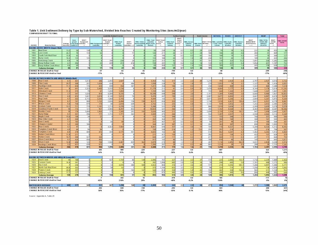
Table 1. Unit Sediment Delivery by Type by Sub-Watershed, Divided Into Reaches Created by Monitoring Sites (tons/mi2/year) COMPARISON DRAFT TO FINAL

NATURAL ROADS HARVEST MGMT Total

BASIN ID Watershed Name Drainage

Area (mi2)

Back­ground

Creep (Deep-Seated LS)

DRAFT Background

Landslides ------­->

FINAL Background Landslides

DRAFT Road-Related

Landslides -----­>

FINAL Road Related

Landslides

DRAFT Harvest

Landslides ----->

FINAL Timber Harvest Related

Landslides

FINAL Total Landslides

(Bkgrd, Roads, Harvest)

DRAFT Road Surface

Erosion ----­->

FINAL Road Sediment Delivery

DRAFT Havest Surface

Erosion ----­->

FINAL Harvest Sediment Delivery

FINAL Bank Erosion

DRAFT TOTAL NATURAL ----­

->

FINAL Landslide + Creep + Bank

Erosion

FINAL Roads ­Landslides &Surface

FINAL Harvest ­Landslides &Surface

DRAFT MANAGEMENT (Road/ Harvest)

------>

FINAL TOTAL ROADS AND

HARVEST RELATED

DRAFT GRAND

TOTAL ---­-->

FINAL GRAND TOTAL

1001 Mud River 13.2 50 138 0 0 0 0 0 50 230 18 0.5 0.5 29 224 79 18 0.5 231 19 455 98 1002 Lost Creek 26.1 70 110 52 0 0 71 4 126 211 26 0.7 0.7 24 186 146 26 4.6 283 31 469 177 1003 South Fork Mad River 15.9 43 5 0 0 0 0 0 43 196 19 0.5 0.5 65 163 108 19 0.5 197 19 360 127 1004 Barry Creek 10.2 133 135 0 0 0 0 0 133 188 44 1.0 1.0 28 234 161 44 1.0 189 45 423 206 1005 Armstrong Creek 9.9 79 5 0 749 230 24 12 321 317 92 1.2 1.2 91 191 170 323 13.2 1,091 336 1,282 506 1006 Deep Hollow Creek 4.1 284 5 23 439 413 414 0 720 201 18 0.4 0.4 14 133 321 431 0.4 1,054 431 1,187 752 1007 Deep Hollow Creek West 4.6 69 5 0 0 0 0 0 69 444 137 1.4 1.4 120 185 189 137 1.4 445 138 630 327

Subarea Average 84 81 74 17 110 47 45 3 148 233 39 0.7 0.7 46 191 144 86 3.4 389 90 580 234

CHANGE IN VALUE-Draft to Final -57 -62 -42 -194 0.0 -48 -299 -346 CHANGE IN PERCENT-Draft to Final -77% -57% -94% -83% -0.5% -25% -77% -60%

1008 Bear Creek 8.1 461 1,013 286 2,093 2,607 0 0 3,354 702 317 2.4 2.3 48 1,219 795 2,924 2.3 2,797 2,927 4,016 3,722 1009 Pilot Creek 39.7 300 201 1,636 424 0 484 2 1,938 228 74 1.0 1.0 17 279 1,953 74 3.1 1,137 78 1,416 2,031 1010 Hastings Creek 11.1 634 176 423 690 354 367 0 1,411 264 106 0.5 0.5 1 258 1,058 460 0.5 1,322 460 1,580 1,518 1011 Holm Creek 8 641 1,323 3,402 3,933 7,136 0 0 11,179 211 41 0.4 0.4 21 1,470 4,064 7,177 0.4 4,144 7,178 5,614 11,242 1012 Olmstead Creek 11.3 575 79 61 1,059 1,093 0 0 1,729 585 250 3.7 3.7 8 193 644 1,343 3.7 1,648 1,347 1,841 1,991 1013 Showers Creek 2.7 547 1,020 816 6,009 9,235 0 0 10,598 648 248 3.0 3.0 6 1,197 1,369 9,483 3.0 6,660 9,486 7,857 10,855 1014 Deer Creek 6.9 653 1,841 3,010 4,140 5,813 76 0 9,476 447 190 4.4 4.5 8 2,007 3,671 6,002 4.5 4,667 6,007 6,674 9,678 1015 Bug Creek 9.7 363 3,772 3,543 1,860 5,193 0 0 9,099 143 73 0.5 0.5 31 3,871 3,937 5,266 0.5 2,004 5,267 5,875 9,204 1016 Morgan Creek 8.7 741 989 1,152 2,826 6,494 138 130 8,517 656 333 0.5 0.5 17 1,158 1,910 6,827 130.4 3,621 6,957 4,779 8,867 1017 Wilson Creek 9.4 750 979 174 80 2,818 649 0 3,742 512 235 0.8 0.8 15 1,143 939 3,052 0.8 1,242 3,053 2,385 3,992 1018 Graham Creek 13.1 711 719 1,191 1,713 3,378 152 0 5,280 531 278 2.7 2.7 17 880 1,919 3,656 2.7 2,399 3,659 3,279 5,578 1019 Goodman Prairie Creek 10 775 121 951 2,905 8,297 855 0 10,023 541 266 0.5 0.5 16 285 1,742 8,564 0.5 4,302 8,564 4,587 10,306 1020 Boulder Creek 19 176 1,604 1,963 173 1,345 291 142 3,626 483 211 0.3 0.3 20 1,698 2,159 1,556 142.1 947 1,698 2,645 3,857 1021 Barry Ridge 9.1 501 396 777 1,715 1,771 363 0 3,049 475 266 5.2 5.2 29 554 1,307 2,037 5.2 2,558 2,042 3,112 3,349 1022 Maple Creek 15.6 100 34 22 0 0 0 0 122 765 348 2.7 2.7 33 132 155 348 2.7 768 351 900 506 1023 Blue Slide Creek 6.1 260 5 0 3 3 0 0 263 364 157 1.0 1.1 44 135 304 160 1.1 368 161 503 465 1030 Deer Creek2 7.1 183 5 0 66 68 0 0 251 407 31 0.5 0.5 18 90 201 99 0.5 474 100 564 301 1031 Showers Creek2 5.2 289 106 55 0 0 0 0 344 881 387 9.2 9.1 19 203 363 387 9.1 890 396 1,093 759 1032 Bear Creek2 4.1 97 5 0 4,563 7,964 0 0 8,061 640 357 4.8 4.8 19 104 116 8,321 4.8 5,208 8,326 5,312 8,442 1033 Tompkins Creek West 4.9 64 96 94 0 0 0 0 158 500 214 1.2 1.2 133 293 291 214 1.2 501 216 794 507 1034 Tompkins Creek 8.9 378 409 472 359 3,175 941 0 4,025 102 26 0.3 0.3 12 510 862 3,201 0.3 1,402 3,202 1,912 4,064 1035 Hetten Creek West 11.9 211 5 0 0 0 0 0 211 421 156 0.7 0.7 11 202 222 156 0.7 422 157 624 379 1036 Hetten Creek 10.7 300 327 344 0 0 0 0 644 247 111 0.3 0.3 0 417 644 111 0.3 247 111 664 755 1037 Olsen Creek West 9.1 424 456 493 0 0 0 0 917 145 40 0.3 0.3 53 700 970 40 0.3 145 41 845 1,011 1038 Olsen Creek 12.8 406 125 704 1,928 2,407 829 362 3,879 273 88 1.3 1.3 6 207 1,116 2,495 362.9 3,031 2,858 3,238 3,974 1039 Hastings Creek West 3.2 651 430 615 0 0 0 0 1,266 287 28 0.5 0.5 48 865 1,314 28 0.5 288 28 1,153 1,342

Subarea Average 266 410 601 986 1,090 2,080 261 32 3,508 411 174 1.6 1.6 21 730 1,418 2,254 34 1,764 2,287 2,494 3,705 CHANGE IN VALUE-Draft to Final 385 989 -229 -237 0.0 687 523 1,211 CHANGE IN PERCENT-Draft to Final 64% 91% -88% -58% 0.6% 94% 30% 49%

1024 Devil Creek 19 188 5 0 927 1,759 84 149 2,096 701 327 4.3 4.3 37 173 225 2,085 153.7 1,716 2,239 1,889 2,464 1025 Cannon Creek 16.4 281 7 1 0 0 0 0 282 1,096 683 5.0 5.0 16 70 298 683 5.0 1,101 688 1,171 986 1026 Dry Creek 7 246 5 0 13 4,076 384 500 4,822 804 316 4.7 4.6 28 177 274 4,392 505.1 1,206 4,897 1,383 5,171 1027 North Fork Mad River 48.8 302 18 9 58 62 1 0 373 1,194 653 3.3 3.3 13 98 324 714 3.5 1,256 718 1,354 1,042 1028 Powers Creek 20.8 397 5 0 0 0 145 147 544 814 358 5.8 5.8 45 155 442 358 152.4 965 511 1,120 953 1029 Lindsay Creek 17.7 177 5 0 0 0 0 0 177 875 440 8.6 8.6 23 108 200 440 8.6 884 448 992 648

Subarea Average 130 278 10 4 158 501 57 72 855 984 514 4.9 4.8 24 120 306 1,015 77 1,204 1,092 1,324 1,398 CHANGE IN VALUE-Draft to Final -7 343 16 -470 0.0 185 -111 74 CHANGE IN PERCENT-Draft to Final -65% 216% 28% -48% -0.2% 154% -9% 6%

WATERSHED AVERAGE 480 317 349 551 667 1,298 168 38 2,203 535 242 2.3 2.3 26 471 894 1,540 40 1,372 1,580 1,843 2,474 CHANGE IN VALUE-Draft to Final 202 630 -130 -292 0.0 423 208 631 CHANGE IN PERCENT-Draft to Final 58% 95% -77% -55% 0.1% 90% 15% 34%

Surface Erosion Landslide Related Erosion Bank Erosion

BASINS ABOVE MRRTH (Upper Mad)

BASINS BETWEEN MRRTH AND MRBVR (Middle Mad)

BASINS BETWEEN MRBVR AND MRALM (Lower/NF)

Source: Appendix A, Table 29

50

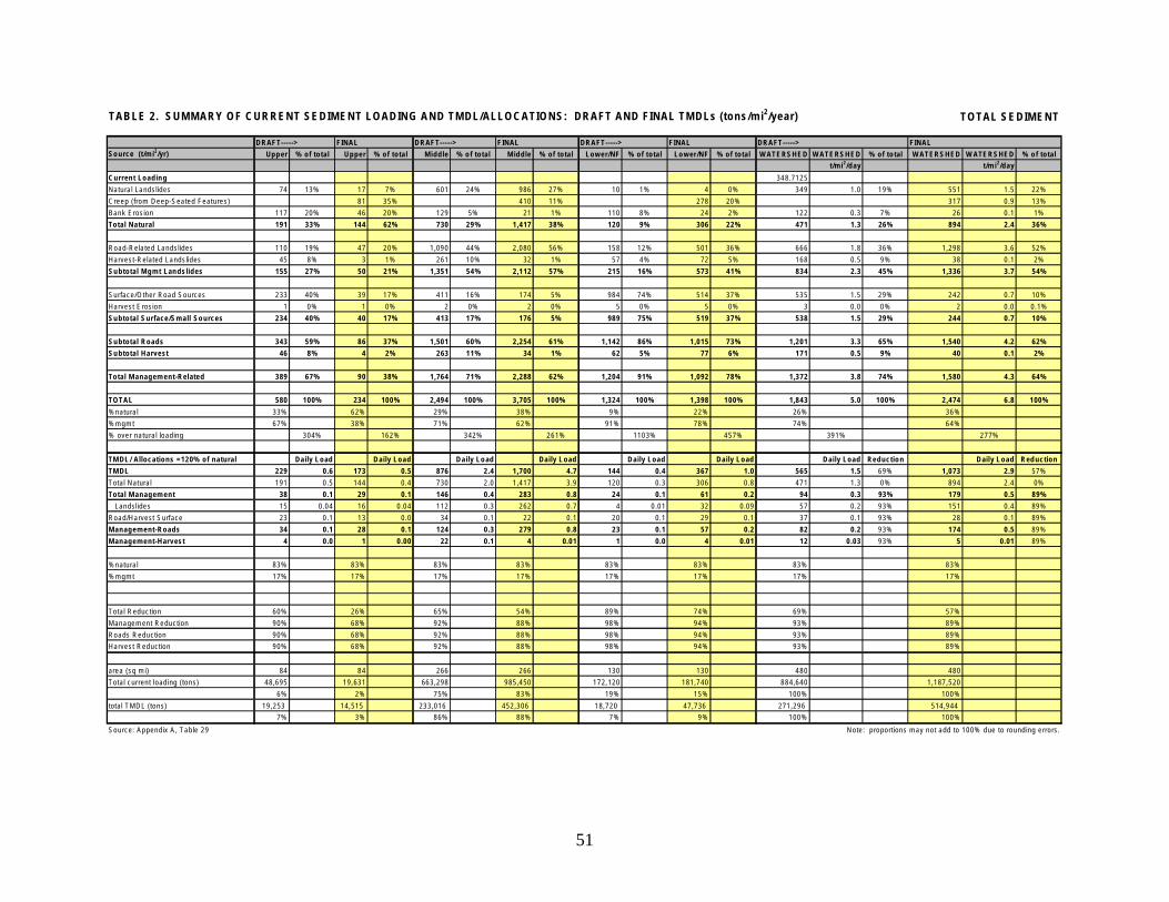
TABLE 2. SUMMARY OF CURRENT SEDIMENT LOADING AND TMDL/ALLOCATIONS: DRAFT AND FINAL TMDLs (tons/mi2/year) TOTAL SEDIMENT

DRAFT-----> FINAL DRAFT-----> FINAL DRAFT-----> FINAL DRAFT-----> FINAL

Source (t/mi2/yr) Upper % of total Upper % of total Middle % of total Middle % of total Lower/NF % of total Lower/NF % of total WATERSHED WATERSHED % of total WATERSHED WATERSHED % of total

t/mi2/day t/mi2/day

Current Loading 348.7125

Natural Landslides 74 13% 17 7% 601 24% 986 27% 10 1% 4 0% 349 1.0 19% 551 1.5 22%

Creep (from Deep-Seated Features) 81 35% 410 11% 278 20% 317 0.9 13%

Bank Erosion 117 20% 46 20% 129 5% 21 1% 110 8% 24 2% 122 0.3 7% 26 0.1 1%

Total Natural 191 33% 144 62% 730 29% 1,417 38% 120 9% 306 22% 471 1.3 26% 894 2.4 36%

Road-Related Landslides 110 19% 47 20% 1,090 44% 2,080 56% 158 12% 501 36% 666 1.8 36% 1,298 3.6 52%

Harvest-Related Landslides 45 8% 3 1% 261 10% 32 1% 57 4% 72 5% 168 0.5 9% 38 0.1 2%

Subtotal Mgmt Landslides 155 27% 50 21% 1,351 54% 2,112 57% 215 16% 573 41% 834 2.3 45% 1,336 3.7 54%

Surface/Other Road Sources 233 40% 39 17% 411 16% 174 5% 984 74% 514 37% 535 1.5 29% 242 0.7 10%

Harvest Erosion 1 0% 1 0% 2 0% 2 0% 5 0% 5 0% 3 0.0 0% 2 0.0 0.1%

Subtotal Surface/Small Sources 234 40% 40 17% 413 17% 176 5% 989 75% 519 37% 538 1.5 29% 244 0.7 10%

Subtotal Roads 343 59% 86 37% 1,501 60% 2,254 61% 1,142 86% 1,015 73% 1,201 3.3 65% 1,540 4.2 62%

Subtotal Harvest 46 8% 4 2% 263 11% 34 1% 62 5% 77 6% 171 0.5 9% 40 0.1 2%

Total Management-Related 389 67% 90 38% 1,764 71% 2,288 62% 1,204 91% 1,092 78% 1,372 3.8 74% 1,580 4.3 64%

TOTAL 580 100% 234 100% 2,494 100% 3,705 100% 1,324 100% 1,398 100% 1,843 5.0 100% 2,474 6.8 100%

%natural 33% 62% 29% 38% 9% 22% 26% 36%

%mgmt 67% 38% 71% 62% 91% 78% 74% 64%

% over natural loading 304% 162% 342% 261% 1103% 457% 391% 277%

TMDL/ Allocations =120% of natural Daily Load Daily Load Daily Load Daily Load Daily Load Daily Load Daily Load Reduction Daily Load Reduction

TMDL 229 0.6 173 0.5 876 2.4 1,700 4.7 144 0.4 367 1.0 565 1.5 69% 1,073 2.9 57%

Total Natural 191 0.5 144 0.4 730 2.0 1,417 3.9 120 0.3 306 0.8 471 1.3 0% 894 2.4 0%

Total Management 38 0.1 29 0.1 146 0.4 283 0.8 24 0.1 61 0.2 94 0.3 93% 179 0.5 89%

Landslides 15 0.04 16 0.04 112 0.3 262 0.7 4 0.01 32 0.09 57 0.2 93% 151 0.4 89%

Road/Harvest Surface 23 0.1 13 0.0 34 0.1 22 0.1 20 0.1 29 0.1 37 0.1 93% 28 0.1 89%

Management-Roads 34 0.1 28 0.1 124 0.3 279 0.8 23 0.1 57 0.2 82 0.2 93% 174 0.5 89%

Management-Harvest 4 0.0 1 0.00 22 0.1 4 0.01 1 0.0 4 0.01 12 0.03 93% 5 0.01 89%

%natural 83% 83% 83% 83% 83% 83% 83% 83%

%mgmt 17% 17% 17% 17% 17% 17% 17% 17%

Total Reduction 60% 26% 65% 54% 89% 74% 69% 57%

Management Reduction 90% 68% 92% 88% 98% 94% 93% 89%

Roads Reduction 90% 68% 92% 88% 98% 94% 93% 89%

Harvest Reduction 90% 68% 92% 88% 98% 94% 93% 89%

area (sq mi) 84 84 266 266 130 130 480 480

Total current loading (tons) 48,695 19,631 663,298 985,450 172,120 181,740 884,640 1,187,520

6% 2% 75% 83% 19% 15% 100% 100%

total TMDL (tons) 19,253 14,515 233,016 452,306 18,720 47,736 271,296 514,944

7% 3% 86% 88% 7% 9% 100% 100%

Source: Appendix A, Table 29 Note: proportions may not add to 100% due to rounding errors.

51

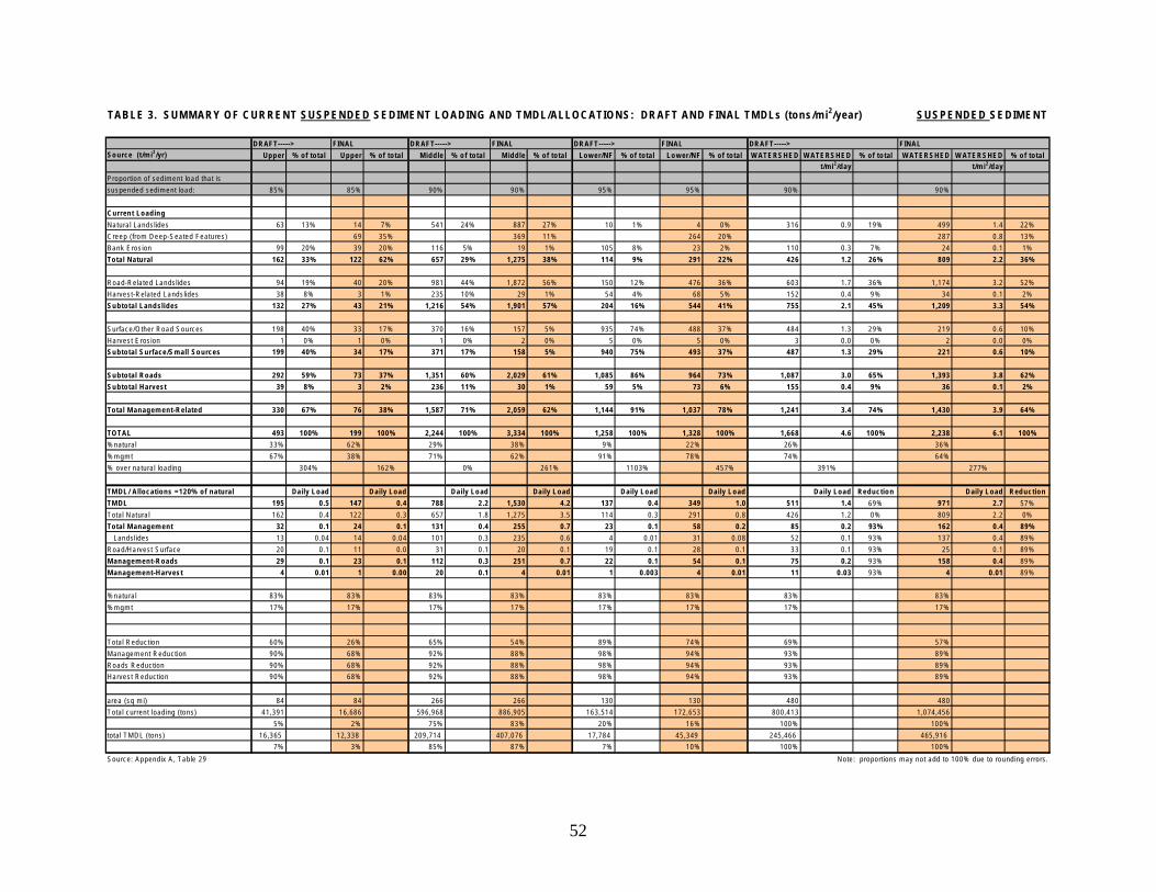
TABLE 3. SUMMARY OF CURRENT SUSPENDED SEDIMENT LOADING AND TMDL/ALLOCATIONS: DRAFT AND FINAL TMDLs (tons/mi2/year) SUSPENDED SEDIMENT

DRAFT-----> FINAL DRAFT-----> FINAL DRAFT-----> FINAL DRAFT-----> FINAL Source (t/mi2/yr) Upper % of total Upper % of total Middle % of total Middle % of total Lower/NF % of total Lower/NF % of total WATERSHED WATERSHED % of total WATERSHED WATERSHED % of total

t/mi2/day t/mi2/day

Proportion of sediment load that is

suspended sediment load: 85% 85% 90% 90% 95% 95% 90% 90%

Current Loading

Natural Landslides 63 13% 14 7% 541 24% 887 27% 10 1% 4 0% 316 0.9 19% 499 1.4 22%

Creep (from Deep-Seated Features) 69 35% 369 11% 264 20% 287 0.8 13%

Bank Erosion 99 20% 39 20% 116 5% 19 1% 105 8% 23 2% 110 0.3 7% 24 0.1 1%

Total Natural 162 33% 122 62% 657 29% 1,275 38% 114 9% 291 22% 426 1.2 26% 809 2.2 36%

Road-Related Landslides 94 19% 40 20% 981 44% 1,872 56% 150 12% 476 36% 603 1.7 36% 1,174 3.2 52%

Harvest-Related Landslides 38 8% 3 1% 235 10% 29 1% 54 4% 68 5% 152 0.4 9% 34 0.1 2%

Subtotal Landslides 132 27% 43 21% 1,216 54% 1,901 57% 204 16% 544 41% 755 2.1 45% 1,209 3.3 54%

Surface/Other Road Sources 198 40% 33 17% 370 16% 157 5% 935 74% 488 37% 484 1.3 29% 219 0.6 10%

Harvest Erosion 1 0% 1 0% 1 0% 2 0% 5 0% 5 0% 3 0.0 0% 2 0.0 0%

Subtotal Surface/Small Sources 199 40% 34 17% 371 17% 158 5% 940 75% 493 37% 487 1.3 29% 221 0.6 10%

Subtotal Roads 292 59% 73 37% 1,351 60% 2,029 61% 1,085 86% 964 73% 1,087 3.0 65% 1,393 3.8 62%

Subtotal Harvest 39 8% 3 2% 236 11% 30 1% 59 5% 73 6% 155 0.4 9% 36 0.1 2%

Total Management-Related 330 67% 76 38% 1,587 71% 2,059 62% 1,144 91% 1,037 78% 1,241 3.4 74% 1,430 3.9 64%

TOTAL 493 100% 199 100% 2,244 100% 3,334 100% 1,258 100% 1,328 100% 1,668 4.6 100% 2,238 6.1 100%

%natural 33% 62% 29% 38% 9% 22% 26% 36%

%mgmt 67% 38% 71% 62% 91% 78% 74% 64%

% over natural loading 304% 162% 0% 261% 1103% 457% 391% 277%

TMDL/ Allocations =120% of natural Daily Load Daily Load Daily Load Daily Load Daily Load Daily Load Daily Load Reduction Daily Load Reduction

TMDL 195 0.5 147 0.4 788 2.2 1,530 4.2 137 0.4 349 1.0 511 1.4 69% 971 2.7 57%

Total Natural 162 0.4 122 0.3 657 1.8 1,275 3.5 114 0.3 291 0.8 426 1.2 0% 809 2.2 0%

Total Management 32 0.1 24 0.1 131 0.4 255 0.7 23 0.1 58 0.2 85 0.2 93% 162 0.4 89%

Landslides 13 0.04 14 0.04 101 0.3 235 0.6 4 0.01 31 0.08 52 0.1 93% 137 0.4 89%

Road/Harvest Surface 20 0.1 11 0.0 31 0.1 20 0.1 19 0.1 28 0.1 33 0.1 93% 25 0.1 89%

Management-Roads 29 0.1 23 0.1 112 0.3 251 0.7 22 0.1 54 0.1 75 0.2 93% 158 0.4 89%

Management-Harvest 4 0.01 1 0.00 20 0.1 4 0.01 1 0.003 4 0.01 11 0.03 93% 4 0.01 89%

%natural 83% 83% 83% 83% 83% 83% 83% 83%

%mgmt 17% 17% 17% 17% 17% 17% 17% 17%

Total Reduction 60% 26% 65% 54% 89% 74% 69% 57%

Management Reduction 90% 68% 92% 88% 98% 94% 93% 89%

Roads Reduction 90% 68% 92% 88% 98% 94% 93% 89%

Harvest Reduction 90% 68% 92% 88% 98% 94% 93% 89%

area (sq mi) 84 84 266 266 130 130 480 480

Total current loading (tons) 41,391 16,686 596,968 886,905 163,514 172,653 800,413 1,074,456

5% 2% 75% 83% 20% 16% 100% 100%

total TMDL (tons) 16,365 12,338 209,714 407,076 17,784 45,349 245,466 465,916

7% 3% 85% 87% 7% 10% 100% 100%

Source: Appendix A, Table 29 Note: proportions may not add to 100% due to rounding errors.

52