Magdalena Alonso Balmaseda, Anderson. Research Department

370

Westerly wind events and the1997 El-Nino event in the

ECMWF seasonal forecastingsystem: a case study

Magdalena Alonso Balmaseda,Frederic Vitart, Laura Ferranti, David

Anderson.

Research Department

11 September 2002

For additional copies please contact

The LibraryECMWFShinfield ParkReadingRG2 [email protected]

Series: ECMWF Technical Memoranda

A full list of ECMWF Publications can be found on our web site under:http://www.ecmwf.int/publications/

c©Copyright 2002

European Centre for Medium Range Weather ForecastsShinfield Park, Reading, RG2 9AX, England

Literary and scientific copyrights belong to ECMWF and are reserved in all countries. This publicationis not to be reprinted or translated in whole or in part without the written permission of the Director.Appropriate non-commercial use will normally be granted under the condition that reference is madeto ECMWF.

The information within this publication is given in good faith and considered to be true, but ECMWFaccepts no liability for error, omission and for loss or damage arising from its use.

http://www.ecmwf.int/publications/

Westerly wind events and the 1997 El-Nino event in . . .

Abstract

The 1997-1998 El-Nino was one of the strongest on record. Its onset was predicted by several numericalmodels, though none fully captured its intensity. This was the case for the ECMWF seasonal forecastingsystem which underestimated the intensification during the period June-July 1997 by more than 1K. Severalstrong westerly wind events developed during the onset of the 1997-1998 El-Nino suggesting that westerlywind events played a key role in the intensification of this El-Nino. The present paper quantifies the impactof westerly wind events on the 1997-1998 El-Nino in the ECMWF seasonal forecasting system, througha series of experiments in which various modifications are made to convective parameterization and windforcing to increase wind variability in the western Pacific.

The first modification to the coupled model involves adding observed wind anomalies to the wind stressderived from the atmospheric model before they are used to force the oceanic component of the coupledmodel. Results indicate that the westerly wind event that occurred in May-June 1997 may have accountedfor a warming of more than 0.5K in the NINO3 region. The second modification, involves adding stochas-tic perturbations to the model tendencies. This produces an increase in the spread of the ensemble and aslightly better forecast of NINO3 sea surface temperatures (SSTs). In a third set of experiments, the convec-tive parameterization of the atmospheric model was modified in order to allow more convective availablepotential energy to accumulate before convection is triggered. This leads to both a significant improvementin the simulation of westerly wind events and in the prediction of the NINO3 SSTs. A few members of theensemble produce a warming in the NINO3 region comparable to the warming produced by the observedwesterly wind burst of May-June 1997.

Ocean-only experiments indicate that the response of the coupled model to the wind perturbation is smallerthan that in forced mode, probably due to the strong damping effect of the induced heat flux. The differentocean mean state does not seem to be responsible for the weak coupled response in the NINO3 region. Therelative importance of anomalies in zonal wind stress, heat flux, precipitation minus evaporation (P-E), andocean initial conditions is determined.

1 Introduction

Predicting El-Nino is a topic of great interest since it is the most important source of potentially predictableinterannual variability. The prediction of its occurrence and development represents a particularly challengingtask for dynamical seasonal forecasting. Several models of intermediate complexity, based on a relativelysimple representation of the Equatorial Pacific Ocean and the tropical atmosphere, have been applied to thistopic with some success. See for example Latif et al 1998 and references therein. The performance of generalcirculation models to predict sea surface temperature anomalies has significantly improved in recent yearsand some of them provided the best real-time numerical forecasts of the 1997-1998 El-Nino (Trenberth 1998)although all the dynamical models considered by Barnston et al. (1999) underestimated the exceptional strengthof the 1997-1998 El-Nino.

The ECMWF seasonal forecasting system, based on coupled General Circulation Models (GCM) integrations,was generally rather successful in predicting the occurrence of the 1997-1998 event, its maintenance and itsdecay, a few months in advance, but forecasts initiated in April and May underestimated its intensification inJune and July 1997 by more than 1K. The main goal of the present paper is to investigate the reasons for thisfailure.

While the El-Nino mode explains most of the interannual variability, tropical intraseasonal variability, whichcan be very intense in some years, is also of interest for seasonal forecasting. For example, the strong El-Ninoevent of 1997 developed during a period of intense intraseasonal activity. Those variations may condition thedevelopment of warm tropical SSTs and therefore may play a substantial role in the onset and development ofthe El-Nino Southern Oscillation (ENSO).

Technical Memorandum No. 370 1


The Madden Julian Oscillation (MJO) is the most dominant and coherent component of the intraseasonal vari-ability in the tropical atmosphere (Madden and Julian 1971, 1972). When it is active it represents a substantialmodulation of the convective activity over the Indian and west Pacific Oceans. Kessler and Kleeman (2000)suggest that the MJO may influence the tropical climate by modulating the timing and strength of ENSO events.Strong MJOs have been observed prior to and during the onset of recent ENSO events, and Kelvin waves gen-erated by MJO forcing in the western Pacific can lead to an increase of sea surface temperatures in the tropicaleastern Pacific. However, the impact of MJOs on ENSO is still questionable since the evidence for a significantstatistical relationship between large-scale MJO activity and ENSO is somewhat contradictory (Hendon et al.1998; Slingo et al. 1998; Bergman et al. 2001; Benestad et al. 2002 ).

Rapid changes in surface winds over the Indonesian region, known as Westerly Wind Bursts (see for instanceHarrison and Giese, 1991) are observed on the intraseasonal time scale. The amplitude of the zonal windanomaly is of the order of a few meters per second. It is still unclear to what extent westerly wind eventsare intimately related to the large-scale MJO phenomenon. Westerly wind events tend to develop during activephases of the MJO (Zhang 1996; Lin and Johnson 1996; Chen et al 1996), though they can also form from pairedtropical cyclones (Keen 1982) and cold surges from midlatitudes (Harrison 1984). Barnett (1984) suggestedthat westerly wind events could affect the ENSO cycle. Slingo (1998), McPhaden (1999) and Boulanger et al.(2001) amongst others have argued that westerly wind events, possibly associated with the MJO, in late 1996and the first half of 1997 played a crucial role in the onset and development of ENSO.

Westerly wind events were present in the western Pacific during the onset of several recent El-Nino events:1990-91, 1992-93, 1993-94, and 1996-97 (Krishnamurti et al 2000). In 1997, before the onset of the strongestEl-Nino recorded, several strong westerly winds events were observed (November 1996, December 1996,February-March 1997). Krishnamurti et al (2000) demonstrate that the initialization of a coupled GCM in-cluding westerly wind events in the ocean data assimilation significantly improved the forecasts of the 1997El-Nino. Perigaud and Cassou (2000), using an intermediate coupled model, argue that the presence of westerlywind events can impact the development of an El-Nino event but only if the oceanic heat content is high, aswas the case in 1997. Therefore, westerly wind events may be an important player in the intensification of the1997 El-Nino event. If this is the case, then it is important for a coupled GCM to be able to generate such windstress variability in order to successfully forecast El-Nino events months in advance.

Simulating a realistic atmospheric intraseasonal variability over the tropical Pacific is still a difficult task forstate-of-the-art GCMs. As part of the Atmospheric Model Intercomparison Project (AMIP; Gates, 1992), Slingoet al. (1996) have compared the MJO variability in fifteen GCMs to the observed variability as represented bythe ECMWF analyses. Their studies showed that the most consistent shortcoming among the models is theweak representation of the strength of the intraseasonal variability. The drastic lack of MJO variability west ofthe dateline in the GCMs may significantly affect their ability to create westerly wind events. It has thereforebeen hypothesized that the failure of GCMs to predict the strong intensity of the 1997-1998 El-Nino event isrelated to their inability to simulate realistic westerly wind events.

This study explores the above hypothesis in the context of the ECMWF seasonal forecasting system. Section 2documents the ECMWF seasonal predictions of the 1997-1998 El-Nino, and the ability of the ECMWF coupledsystem to simulate realistic MJOs and westerly wind events. In Section 3, results from sensitivity experimentsusing fully coupled GCMs and designed to evaluate the impact of westerly wind events on the El-Nino 1997 arediscussed. Section 4 shows that there is large sensitivity to a specific change in the cumulus parameterizationscheme. Results from these experiments indicate that the significant improvement in predicting the SST anoma-lies over the NINO3 region (150W-90W, 5N-5S) for the 1997-1998 El Nino is related to the enhancement oftropical intraseasonal activity in the model. The relative importance of the wind and heat flux variability in theamplitude of SST anomalies is considered in Section 5 by means of ocean-only experiments. Summary andconclusions are presented in Section 6.

2 Technical Memorandum No. 370


2 Seasonal predictions of NINO3 SST anomalies and simulation of intrasea-sonal activity

The ECMWF seasonal forecasting system (Stockdale et al 1998) is based on a coupled GCM that has been usedto make an ensemble of 6-month forecasts every month from 1991 to present. The atmospheric component (IFScycle 15R8) has a T63 spectral resolution and a 1.875o grid for surface and physical processes; there are 31vertical levels. The ocean resolution is comparable in mid-latitudes, but is increased in the tropics to about0.5o in the latitudinal direction, so as to resolve the equatorial waves which are important for El-Nino. Thereare 20 vertical levels of which eight are in the upper 200 meters. The atmospheric and land surface initialconditions are taken from the operational analyses/reanalyses produced by ECMWF. Ocean initial conditionsare taken from an analysis of the ocean state made by forcing the ocean with the analyzed surface fluxesof momentum, fresh water and heat while assimilating all available subsurface thermal ocean data using theoptimal interpolation scheme of Smith et al (1991) and relaxing to surface temperature analyses (Reynolds andSmith 1994).

The ECMWF seasonal forecasting system displays skill in predicting SST anomalies over the NINO3 region:fig 1 shows that the system was successful in forecasting the onset of the 1997 El-Nino event and its decay.For forecasts started in April and May, however, the model severely underestimated the intensity of the SSTwarming during the months of June and July. This result is consistent with other GCM forecasts (Barnston etal 1999, Landsea and Knaff 2000).

The period from December 1996 to June 1997 was characterized by strong tropical intraseasonal activity withinwhich were very energetic westerly wind events (McPhaden 1999, Slingo 1998). It is likely that such strongwesterly wind events perturbed significantly the equatorial ocean by creating oceanic Kelvin-waves and pos-sibly intensifying the El-Nino (McPhaden 1999). The seasonal forecast system is generally deficient in repre-senting tropical intraseasonal activity. In fact, westerly wind anomalies propagate eastwards only when theyare present in the initial conditions. This is illustrated by Figure 2 for forecasts initiated in February and March1997. Comparison of the analysis of fig 2a with the forecasts in fig 2b, shows that the wind events of mid-February and especially March were not reproduced in forecasts started at the beginning of February. On theother hand fig 2c shows that some aspects of the March event were captured in forecasts started on 1 March.

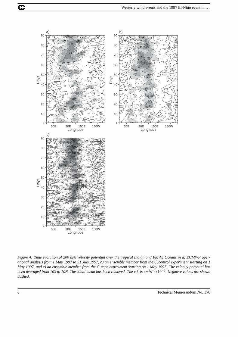
Figure 3a shows strong westerly wind events that developed from May to mid-June 1997 and propagated east-ward from the Indian Ocean to as far east as 150W, with an intensity exceeding 0.08Nm−2. For forecastsstarted on 1 May 1997, not one single member of the 30-member ensemble of the ECMWF seasonal fore-casting system was able to produce propagating wind events comparable to those observed. Fig 3b shows oneensemble member chosen at random from the coupled control experiment (Ccontrol) which will be introducedin secn 3. It is not just the surface winds that do not show propagation. Fig 4a shows the velocity potential at200 hPa in the ECMWF analysis, a field that is often used as a measure of MJO activity. Eastward propagationcan be clearly seen. Fig 4b shows just one ensemble member from Ccontrol drawn at random. No eastwardpropagation is evident. Analysis of other ensemble members confirms the absence of eastward propagation ofMJO-like activity.

Ensembles of atmospheric-only integrations initiated with the same atmospheric initial conditions as in thecoupled forecasts (from analyzed atmospheric state, soil moisture and snow cover), and driven by observedSSTs show a similar behaviour. The atmospheric simulations, integrated for several cases including May 1997were unable to create anything close to the observed westerly wind events, except when the wind event waspresent in the initial conditions, suggesting that the lack of westerly wind events in the coupled model stemsfrom a deficiency in the atmospheric model. Several atmospheric integrations have shown that increasinghorizontal resolution of the atmospheric component of the GCM to T95, T159 and T319, does not improve



A1996

M J J A S O N D J1997

F M A M J J-2

-1

0

1

2

3

4

Ano

mal

y (d

eg C

)

O1996

N D J1997

F M A M J J A S O N D J1998

-1

0

1

2

3

4

Ano

mal

y (d

eg C

)

J1997

F M A M J J A S O N D J1998

F M A-1

0

1

2

3

4

5

Ano

mal

y (d

eg C

)

A1997

M J J A S O N D J1998

F M A M J J

-1

0

1

2

3

4

Ano

mal

y (d

eg C

)

ECMWF Forecasts from December 1996 ECMWF Forecasts from April 1997

ECMWF Forecasts from July 1997 ECMWF Forecasts from October 1997

Figure 1: Plumes of monthly mean SST anomalies predicted for the NINO3 region (5oS−5oN, 90oW−150oW). Forecastsare initialized one day apart and run for 184 days. Start dates: December 1996 (top left), April 1997 (top right), July1997 (bottom left) and October 1997 (bottom right). The thick line shows the observed values. Each thin line representsone member of the ensemble.



-7.5-7.5

-7.5-7.5

-2.5

-2.5

-2.5-2.5

-2.5-2.5

-2.5

-2.5

-2.5-2.5

-2.5

-2.5

-2.5

-2.5

-2.5

-2.5-2.5

-2.5

-2.5-2.5

-2.5-2.5

2.5

2.5

2.5

2.5

-7.5-7.5

-2.5-2.5

-2.5-2.5

-2.5

-2.5

-2.5

-2.5

-2.5

-2.5

-2.5-2.5

-2.5

-2.5

-2.5

-2.5

-2.5

-2.5

-2.5-2.5

-2.5-2.5

-2.5-2.5

-2.5-2.5

30E 90E 150E 150WLongitude

20

40

60

Day

s

20

40

60

Day

s

20

40

60

Day

s



a)

c)

b)

B

A

B

A

Figure 2: Time evolution of the zonal wind at 850 hPa over the tropical Indian and Pacific Oceans in a) ECMWF op-erational analysis from 1 February 1997 to 30 March 1997, and in one ensemble member from the operational coupledforecast system (system 1) starting on a) 1 February 1997 and c) 1 March 1997. The westerly wind burst is present in theinitial conditions of the latter forecast. The zonal wind has been averaged from 10S to the Equator. The starting timesof the forecasts are marked on the analysis of panel a, by A and B. The contour interval (c.i.) is 2.5m/s. Dashed linesindicate easterly winds



26 JUL

21 JUL

16 JUL

11 JUL

6 JUL

1 JUL

26 JUN

21 JUN

16 JUN

11 JUN

6 JUN

1 JUN

26 MAY

21 MAY

16 MAY

11 MAY

6 MAY

1 MAY40 80 120 160

a) Analysis

200 240

26 JUL

21 JUL

16 JUL

11 JUL

6 JUL

1 JUL

26 JUN

21 JUN

16 JUN

11 JUN

6 JUN

1 JUN

26 MAY

21 MAY

16 MAY

11 MAY

6 MAY

1 MAY40 80 120 160

b) Control

200 240

26 JUL

21 JUL

16 JUL

11 JUL

6 JUL

1 JUL

26 JUN

21 JUN

16 JUN

11 JUN

6 JUN

1 JUN

26 MAY

21 MAY

16 MAY

11 MAY

6 MAY

1 MAY40 80 120 160

c) CAPE 500

200 240

Figure 3: Time evolution of surface zonal wind stress over the tropical Indian and Pacific Oceans a) in the ECMWFoperational analysis, b) an ensemble member from the Ccontrol experiment and c) an ensemble member from the Ccapeexperiment. The wind stress has been averaged from 5S to 5N. Contours are 0.02, 0.04, 0.06 and 0.1Nm−2. Values below0.02 Nm−2 are not shown.



significantly the simulation of the intraseasonal variability of the wind stress over the tropical Pacific, indicatingthat the problem is not simply one of resolution.

In summary, the tropical intraseasonal activity is severely underestimated in both coupled and uncoupled sim-ulations integrated for 30 days or longer. The model fails to simulate eastward propagation of anomalousconvection from the Indian Ocean to the western and central Pacific. The variability in the western Pacific isweaker in the model compared to observations. This might indicate a deficiency in the parameterization of thephysical processes related to the MJO. Below we will in fact show that the problem occurs within a rather shorttimescale.

At ECMWF, high resolution forecasts are made every day out to 10 days in order to generate medium rangeweather forecasts. These can be used to evaluate the ability of the model to simulate and predict westerly windevents up to 10 days ahead. We will concentrate on the May-June 1997 westerly wind event. Fig 5 shows’Hovmoller’ plots of the surface wind for 1-day, 2-day, 5-day and 10-day forecasts. The dates on figure 5correspond to the verifying time of the forecast. If the model could simulate equatorial winds correctly andthey were predictable, then the 10-day forecasts of fig 5d should look like the analyses- these latter are notshown but in fact the 1-day forecasts of fig 5a are a good proxy as the model does not degrade too much overthe first day of integration. Fig 5 shows that the speed of propagation of the westerly wind event over the IndianOcean gets slower as the forecast-range increases and the amplitude is noticeably reduced (compare 1-dayforecasts in fig 5a with 10-day forecasts in fig 5d for instance). The model fails to predict the transition of thewesterly wind event from the Indian Ocean to the western Pacific more than 2 days in advance. In particular, themodel fails to predict the correct intensity of the westerly wind event over the western Pacific (between 120Eand 140E) during the period 15 May-1st June 48 hours in advance (Fig 5b) and does not predict its occurrenceat all over the western Pacific 5 days in advance (Fig. 5c). However, when the initial conditions include thewesterly wind event in the western Pacific, the model succeeds in predicting its propagation into the centralPacific (between 160E and 140W) 10 days in advance, although it does not extend as far eastward as in theanalysis (Fig 5d).

The predictability of westerly wind events on seasonal time scales is probably not very high. However, if theatmospheric model were able to create westerly wind events, one would expect that within a sufficiently largeensemble, some members of the ensemble would create a westerly wind event at approximately the right timeand with the right intensity. If the June 1997 westerly wind event played a significant role in the developmentof the 1997 El-Nino but its predictability on the seasonal scale was low, then, even with a perfect atmosphericmodel, only a few members of the ensemble would be expected to predict the strong warming in the NINO3region in June-July 1997.

3 Sensitivity of the coupled forecast to the May-June 1997 westerly wind event

Although the intraseasonal activity is largely underestimated by the seasonal forecasts throughout the periodDecember 1996 to June 1997, we will concentrate on the specific case of seasonal predictions initiated in May1997. The 1st May was chosen as a starting date partly because the operational seasonal forecasts from Mayfailed to predict the intensity of the El-Nino and partly because it is close to the observed May-June westerlywind event. By performing additional experiments we will investigate whether part of the seasonal predictionerror could be related to the inadequate representation of westerly wind activity.

All the experiments have been performed using the same ocean component of the coupled GCM as in theoperational seasonal forecasting system but with a more recent version of the atmospheric model (known ascycle 19r1). A 5-member ensemble of 3-month integrations has been generated, in which each one is startedon 1 May for each year from 91-96. These are used to create the reference climatology (CCONTROL CLIM)



4

4

4

4

4

12

-4

-4

-4

-4

-4

-4

-4

10

20

1

30

40

50

60

70

80

90

Day

s


12

-4

-4

-4

4

4

-4

10

20

1

30

40

50

60

70

80

90

Day

s


10

20

1

30

40

50

60

70

80

90D

ays


a)

c)

b)

Figure 4: Time evolution of 200 hPa velocity potential over the tropical Indian and Pacific Oceans in a) ECMWF oper-ational analysis from 1 May 1997 to 31 July 1997, b) an ensemble member from the Ccontrol experiment starting on 1May 1997, and c) an ensemble member from the Ccape experiment starting on 1 May 1997. The velocity potential hasbeen averaged from 10S to 10N. The zonal mean has been removed. The c.i. is4m2s−1x10−6. Negative values are showndashed.



26 JUL

21 JUL

16 JUL

11 JUL

6 JUL

1 JUL

26 JUN

21 JUN

16 JUN

11 JUN

6 JUN

1 JUN

26 MAY

21 MAY

16 MAY

11 MAY

6 MAY

1 MAY40E 80E 120E 120W160E 160W

a) 1-day forecasta) 1-day forecast

c) 5-day forecast

26 JUL

21 JUL

16 JUL

11 JUL

6 JUL

1 JUL

26 JUN

21 JUN

16 JUN

11 JUN

6 JUN

1 JUN

26 MAY

21 MAY

16 MAY

11 MAY

6 MAY

1 MAY40E 80E 120E 120W160E 160W

b) 2-day forecast

26 JUL

21 JUL

16 JUL

11 JUL

6 JUL

1 JUL

26 JUN

21 JUN

16 JUN

11 JUN

6 JUN

1 JUN

26 MAY

21 MAY

16 MAY

11 MAY

6 MAY

1 MAY40E 80E 120E 120W160E 160W

26 JUL

21 JUL

16 JUL

11 JUL

6 JUL

1 JUL

26 JUN

21 JUN

16 JUN

11 JUN

6 JUN

1 JUN

26 MAY

21 MAY

16 MAY

11 MAY

6 MAY

1 MAY40E 80E 120E 120W160E 160W

d) 10-day forecast

Figure 5: Time evolution of wind stress from a) 1-day, b) 2-day, c) 5-day and d) 10-day forecasts from the ECMWFmedium-range operational forecast system. C.i. is0.02Nm−2. Only positive values are shown, starting at0.02Nm−2.



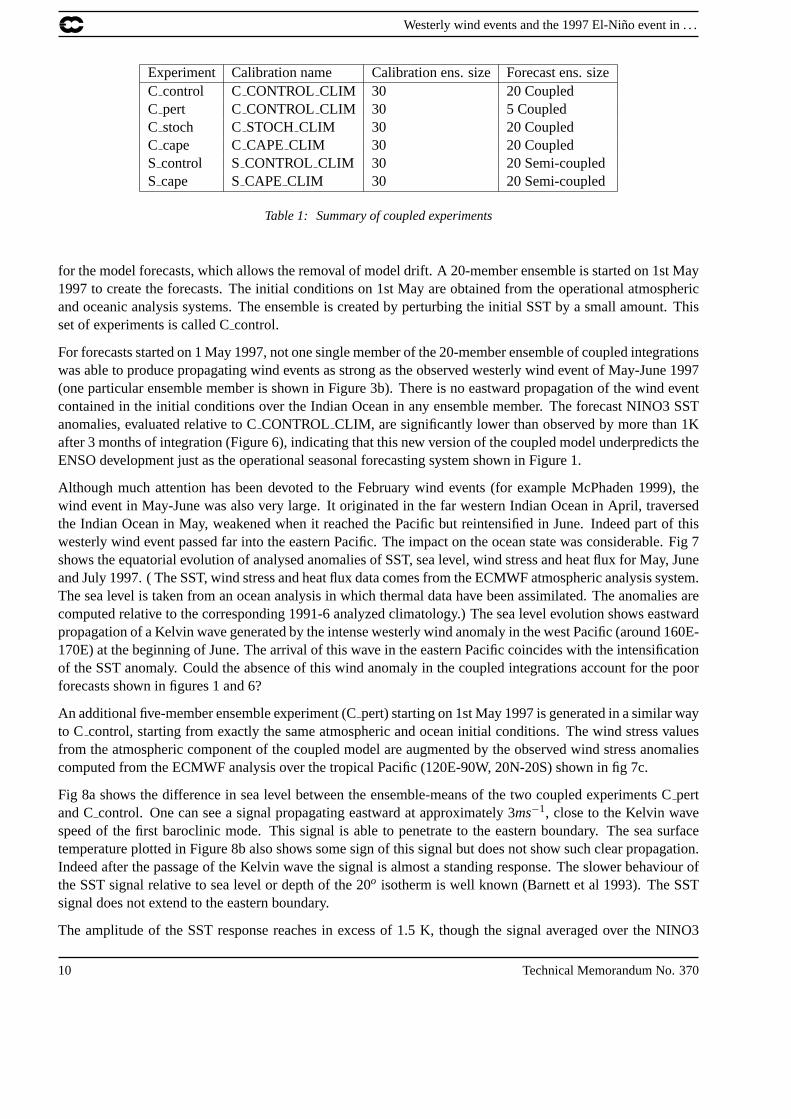
Experiment Calibration name Calibration ens. size Forecast ens. sizeC control C CONTROL CLIM 30 20 CoupledC pert C CONTROL CLIM 30 5 CoupledC stoch C STOCHCLIM 30 20 CoupledC cape C CAPE CLIM 30 20 CoupledS control S CONTROL CLIM 30 20 Semi-coupledS cape S CAPE CLIM 30 20 Semi-coupled

Table 1: Summary of coupled experiments

for the model forecasts, which allows the removal of model drift. A 20-member ensemble is started on 1st May1997 to create the forecasts. The initial conditions on 1st May are obtained from the operational atmosphericand oceanic analysis systems. The ensemble is created by perturbing the initial SST by a small amount. Thisset of experiments is called Ccontrol.

For forecasts started on 1 May 1997, not one single member of the 20-member ensemble of coupled integrationswas able to produce propagating wind events as strong as the observed westerly wind event of May-June 1997(one particular ensemble member is shown in Figure 3b). There is no eastward propagation of the wind eventcontained in the initial conditions over the Indian Ocean in any ensemble member. The forecast NINO3 SSTanomalies, evaluated relative to CCONTROL CLIM, are significantly lower than observed by more than 1Kafter 3 months of integration (Figure 6), indicating that this new version of the coupled model underpredicts theENSO development just as the operational seasonal forecasting system shown in Figure 1.

Although much attention has been devoted to the February wind events (for example McPhaden 1999), thewind event in May-June was also very large. It originated in the far western Indian Ocean in April, traversedthe Indian Ocean in May, weakened when it reached the Pacific but reintensified in June. Indeed part of thiswesterly wind event passed far into the eastern Pacific. The impact on the ocean state was considerable. Fig 7shows the equatorial evolution of analysed anomalies of SST, sea level, wind stress and heat flux for May, Juneand July 1997. ( The SST, wind stress and heat flux data comes from the ECMWF atmospheric analysis system.The sea level is taken from an ocean analysis in which thermal data have been assimilated. The anomalies arecomputed relative to the corresponding 1991-6 analyzed climatology.) The sea level evolution shows eastwardpropagation of a Kelvin wave generated by the intense westerly wind anomaly in the west Pacific (around 160E-170E) at the beginning of June. The arrival of this wave in the eastern Pacific coincides with the intensificationof the SST anomaly. Could the absence of this wind anomaly in the coupled integrations account for the poorforecasts shown in figures 1 and 6?

An additional five-member ensemble experiment (Cpert) starting on 1st May 1997 is generated in a similar wayto C control, starting from exactly the same atmospheric and ocean initial conditions. The wind stress valuesfrom the atmospheric component of the coupled model are augmented by the observed wind stress anomaliescomputed from the ECMWF analysis over the tropical Pacific (120E-90W, 20N-20S) shown in fig 7c.

Fig 8a shows the difference in sea level between the ensemble-means of the two coupled experiments Cpertand Ccontrol. One can see a signal propagating eastward at approximately 3ms−1, close to the Kelvin wavespeed of the first baroclinic mode. This signal is able to penetrate to the eastern boundary. The sea surfacetemperature plotted in Figure 8b also shows some sign of this signal but does not show such clear propagation.Indeed after the passage of the Kelvin wave the signal is almost a standing response. The slower behaviour ofthe SST signal relative to sea level or depth of the 20o isotherm is well known (Barnett et al 1993). The SSTsignal does not extend to the eastern boundary.

The amplitude of the SST response reaches in excess of 1.5 K, though the signal averaged over the NINO3



Figure 6: Plume of monthly mean SST anomalies predicted for the NINO3 region. Forecasts start on 1st May 1997,and the 20-member ensemble is generated by adding small perturbations to the initial SSTs. The squares represent theobserved values, the circles represent the ensemble distribution for the experiment Ccontrol, and the diamonds representthe ensemble distribution for Cpert. The values are plotted at the middle of the month.



Longitude

Tim

e (d

ays)

1

1

2�

2

2� .5�

2.5

3

3�

3�

3.5

3.5

4

110°E 130°E 150°E 170°E 170°W 150°W 130°W 110°W 9�

0°W 7�

0°W

Longitude110°E 130°E 150°E 170°E 170°W 150°W 130°W 110°W 9

�0°W 7

�0°W


�0°W 7

�0°W

0.05

0.10.15

0.2

0.2 0�

.2�

0.25

0.25

0

20

40

6

0

8�

0

Tim

e (d

ays)


�0°W 7

�0°W

0

20

40

6

0

8�

0

Tim

e (d

ays)

0

20

40

6

0

8�

0

Tim

e (d

ays)

0

20

40

6

0

8�

0

-0.02

-0.02

0.020.02

0�

.02

0

.02

0�

.02

0�

.04

0.04

0.040.04

0.060.08

0.08

-100

-50

-50

-50

-50�

-50

-50

a b

c d

Figure 7: Time evolution (from 1st May 1997 to 1st August 1997) of the analysed anomalies of equatorial a) SST, b) sealevel c) zonal wind stress, and d) heat flux; all are with respect to the analyzed 1991-1996 climatology. Only the Pacificbasin is shown. c.i. is 0.5K, 0.5m, 0.02 Nm−2, and 50Wm−2 respectively. Values above 0.5K, 0.1m, 0.02 Nm−2 areshaded in panels a,b and c. Negative values are shaded in panel d.



110OE 130OE 150OE 170OE 170OW 150OW 130OW 110OW 90OW 70OW

Longitude0

20

40

60

80

Tim

e (d

ays)

0

20

40

60

80

aSea level contoured every 0.05 mCoupled: PERT - CNTL

I.C. 19970501

0.05�

0.05�

0.05�

0.05�

0.1

0.1

0.15

0.15�

MAGICS 6.3 tamlane - neh Sun Apr 21 17:29:59 2002


Longitude0

20

40

60

80

Tim

e (d

ays)

0

20

40

60

80

bPotential temperature contoured every 0.5 deg CCoupled: PERT - CNTL

I.C. 19970501

0.5

0.5

0.5

0.50.5

1


Figure 8: a) Time evolution of ensemble mean difference in equatorial Pacific sea surface height (m) between Cpert andC control. Start date is 1st May 1997. Shading indicates values greater than 0.1m. c.i. is 0.05m. b) As for (a) but forpotential temperature. Shading indicates values greater than 0.5K. c.i. is 0.5K



region is less than this value since it includes a region where the SST signal is weak. Figure 6 shows thepredicted SST anomalies in NINO3 from the coupled experiment Cpert. One can see that the latter forecastsare considerably better than those in Ccontrol but are still weaker than the observed amplitude.

The changes in SST induced by the imposed winds in turn generate new winds and heat fluxes. Figures 9aand 9b show the changes in wind and heat flux induced by the SSTs resulting from the wind perturbation,and illustrate the character of the coupled interactions in the model. Over the Central and Eastern Pacific, thestresses are broadly in line with expectation in that there is anomalous convergence over the area of warm SSTanomalies. The effect of these winds on SST will be discussed in secn 5.2.

One might have guessed that the development of such a large El-Nino as 1997 would have had some help fromthe heat fluxes during the development phase ( i.e. a positive heat flux anomaly) but it appears that this wasnot so in the coupled model. The observed SST and heat flux anomalies from the ECMWF analysis system areshown in figures 7a and 7d respectively. They confirm that the heat flux was negative throughout this period.The ratio between heat flux anomalies and SST anomalies for the Cpert experiment is about−80Wm−2K−1

over the eastern Pacific, with a close link between the regions of maximum anomalous SST and maximumheat flux (cf figs 8b and 9b). The spatial structure of the analysed heat flux in fig 7d does not mirror the SSTanomaly of Figure 7a to the same extent as in the Cpert experiment, and the link between anomalous SSTand anomalous heat flux in the analysis seems weaker than in the coupled model, at about−40Wm−2K−1,suggesting that the negative feedback from the heat flux in the coupled model may be too strong. The role ofheat fluxes will be discussed further in Section 5.

The above experiments suggest that the westerly wind event of June 1997 had a significant impact on theintensification of the 1997 El-Nino and that part of the failure of the coupled GCM to predict the strength ofthe El-Nino event can be explained by its inability to produce a significant variability in the wind stress forcing.This result does not exclude the possibility that errors in the ocean model, in the model climatology (which isdefined from only six different years) or errors in the initial conditions are also important contributions to theinaccuracy of seasonal predictions. The effects of ’additional’ errors will not be discussed further in this sectionsince the main focus is to find if there is any relationship between the warming in the NINO3 region and theMay-June westerly wind event.

The previous experiments suggest that it is necessary for the atmospheric model to simulate westerly windevents in order to be successful in simulating the intensification of the 1997 El-Nino event. Several methods ofincreasing the model variability are possible. One consists of adding stochastic perturbations to each memberof the ensemble throughout the duration of the forecast. An example of such a technique is the use of stochasticphysics (Palmer 2001), where tendencies in the atmospheric model are randomly perturbed. A 20 memberensemble of forecasts with stochastic physics was performed starting on the first of May 1997. This will bedenoted Cstoch. Since stochastic physics might perturb the model reference climatology, a new set of hindcastsspanning the period 1991-6 was necessary. This climatology is denoted CSTOCHCLIM. The 97 anomaliesmeasured relative to this climatology are shown in fig 10a. Comparison with fig 6 indicates a spread of Cstochensemble much larger than in the Ccontrol. Several members of the ensemble display a warming strongerthan any member of the Ccontrol run, and not too far from the warming obtained when adding observed windperturbations. No member approaches the observed warming, however.

While stochastic physics creates perturbations of the surface wind, it is unlikely that these will resemble west-erly wind events. Stochastic physics perturbations would be applied independently of the fact that we knowthere will be a westerly wind event, and therefore a part of the predictability is lost. Modifying the physics ofthe atmospheric model in such a way that it can create and maintain westerly wind events should be a betterapproach, since any predictability of westerly wind events would then be taken into account. The next sectionexplores this approach.




Longitude0

20

40

60

80

Tim

e (d

ays)

0

20

40

60

80

aTaux contoured every 0.02 PaEffect of coupling

I.C. 19970501

0.02�



Longitude0

20

40

60

80

Tim

e (d

ays)

0

20

40

60

80

bHeat Flux contoured every 20 Watt/mEffect of coupling

I.C. 19970501

-80

-60�

-60

-60�

-40�

-40�

-40�

-40�

-20�

-20-20

-20

20

40 60


Figure 9: Equatorial Hovmuller diagram of the coupled response to the wind perturbation (τpert). a) Coupled response interms of zonal wind stress (τ), defined asτC pert−(τC control+τpert). b) The heat flux (H f lx) coupled response, defined asH f lxC pert−H f lxC control. Plots show the average of 5 ensemble members. In a) shading indicates values greater than0.02Nm−2 and the c.i. is0.02Nm−2. In b) negative values are shaded and the c.i. is20Wm−2.



Figure 10: Plume of monthly mean SST anomalies predicted for the NINO3 region (5oS−5oN, 90o−150oW). Forecastsare initialized on 1st May 1997, and the 20-member ensemble is for experiments a) Cstoch and b) Ccape. The squaresrepresent the observed values.

4 Sensitivity of coupled forecasts to changes in cumulus parameterization

The deep convection scheme used in the present model is a mass-flux scheme described in Tiedtke(1989).The scheme is designed to minimize the Convective Available Potential Energy (CAPE), the closure beingthe condition that the CAPE should be zero. There is no observational evidence that such a condition shouldapply in the real world. Increasing the threshold of the CAPE is known to significantly impact the transientsin the model (Tokioka 1988, Vitart et al 2001). Lin and Neelin (2000) have proposed using different values ofthe CAPE threshold to generate an ensemble of perturbations. Tests with different values of CAPE thresholdindicate that the change in the convective parameterization becomes significant when the CAPE thresholdexceeds a value of the order of 200JKg−1. As the main focus of the following experiments is to find out if thevariability of the ECMWF model is sensitive to the CAPE threshold, a value of 500JKg−1 was chosen, thoughthis may be higher than can be rigorously justified. The choice of 500JKg−1 for the CAPE thershold will bereferred as CAPE500 hereafter.

Part of the failure of the present system to develop intraseasonal variability may be due to the fact that thesimulated atmosphere is too stable. Having a CAPE threshold greater than zero delays the onset of deepconvective adjustment parametrisation allowing the model to become more unstable and to perform more ofthis role explicitly. This may help the model to develop intraseasonal variability.

4.1 Results from coupled integrationsAs for the previous experiments, a 20-member-ensemble of 3-month integrations starting on 1st May 1997has been generated with the CAPE500 choice (Ccape runs). In addition, a calibration set consisting of 5-



member ensembles of coupled integrations using the same CAPE500 threshold and starting on 1st May 1991to 1996 has been created to sample the related climatology CCAPE CLIM. Changes in the physics of themodel have a significant impact on the mean state and on the drift of the coupled model. For example, theSST of CCAPE CLIM is colder than that of CCONTROL CLIM in the NINO3 region (Fig. 11). Theatmospheric mean state simulated by the CCAPE CLIM is not significantly better than the one from theC CONTROL CLIM. The impact of delaying the convective activity depends on the season. Additional ex-perimentation based on uncoupled simulations has shown that winter CAPE500 simulations have an improvedmean atmospheric circulation but those started in spring-summer showed a degraded mean circulation.

The Ccape experiments increase significantly the variability of the wind stress over the tropical Pacific.Whereas the Ccontrol runs were unable to create strong eastward propagation of wind events in the Centralwestern Pacific, Ccape runs can create westerly wind events near the dateline with an amplitude comparable toobservations. Fig. 3c shows one such example. The eastward propagation can also be seen in terms of velocitypotential at 200hPa from a coupled Ccape integration starting on 1st May 1997 (fig 4c). The eastward dis-placement of deep convection in the Tropical Pacific is reminiscent of the Madden-Julian Oscillation, thoughthe speed of propagation is too large. This seems to be a clear improvement in comparison to experimentC control (fig 4b), though still not fully realistic. However, not a single member of the 20-member ensembleof C cape started on 1 May 1997 creates a westerly wind event extending as far eastward as observed in June1997. Nevertheless, the Ccape experiments can be used as sensitivity experiments to evaluate the impact ofwesterly events on the SST variability. The 20-member Ccape ensemble initiated on 1st May 1997 shown inFigure 10b displays a warming of SST significantly larger than the control ensembles (Fig. 6) (95% significantaccording to the Wilcoxson-Mann-Whitney test, e.g. Wonnacott and Wonnacott 1997) . The ensemble mean isstill far from the observed warming, but some members of the ensemble create a warming close to that obtainedwhen the observed westerly wind anomalies are imposed on the ocean.

All 20 members of the ensemble predict westerly wind events in the first two months of integrations, thoughthe intensity and timing varies considerably from one member to the next. The ensemble members that createthe strongest warming over NINO3 coincide with the members exhibiting the strongest westerly wind events.Three-month averages of NINO3 SSTs and zonal winds averaged over the Central Pacific region (160E-180Eand 5N-5S) are significantly correlated (correlation of 0.7), suggesting that the westerly wind events in themodel have a significant impact on the NINO3 SSTs. Fig 12 shows a Hovmuller diagram of the time evolutionof the difference in SSTs, sea level and wind stress between the best Ccape and the best Ccontrol (bestmeaning the ensemble members that produced the strongest warming in the NINO3 region). The difference inNINO3 SSTs between the two sets of experiments can be traced back to the occurrence of two westerly windevents, in May and June, that propagated eastward well beyond the dateline. The impact of those westerlywind events on the ocean state can be seen in the sea level (fig 12b) as eastward propagating Kelvin waves andin the SST warming that appears to the east of the wind anomaly (figure 12c). This suggests that the abilityof C cape simulations to create westerly wind events is the main reason for the improvement in the NINO3forecasts. Some improvements with Ccape may be due to a different mean state as shown in Figure 11. In thefollowing section, we will consider the impact of the drift, and in section 5.2 we will evaluate the impact of thewind variability produced in Ccape when acting on a different oceanic mean state, with experiments involvingocean-only runs.

4.2 Results from ’semi’-coupled integrations

To evaluate the influence of the SST drift in figure 11 on the NINO3 forecasts shown in figure 10, experimentshave been generated in which the atmosphere sees the observed SSTs, whereas the ocean is forced by thefluxes produced by the atmosphere. Two sets of experiments, Scape and Scontrol, have been generated with



MAY�

JUNE�

JULY25.5

26.0

26.5

27.0

27.5

SS

Ts

�

Mean SSTs (1991−1996) over NINO3

OBSControlCAPE500

Figure 11: Mean SSTs averaged over the NINO3 region and over the period 1991-1996. The squares represent theobserved mean SSTs, the circles, the mean of the Ccontrol integrations starting on 1st May and the diamonds the meanof the Ccape integrations starting on 1st May.

and without the change in the CAPE threshold. The results obtained in this framework are consistent withthose obtained when the atmosphere and ocean are fully coupled; i.e. in experiments Scape the SST warmingproduced by the ocean model in the NINO3 region is significantly larger than in the corresponding Scontrolexperiments. Since the atmosphere is driven by observed SSTs in these experiments, the drift in SSTs in theocean model has no impact on the simulated atmospheric intraseasonal variability. Therefore, the difference inthe SST anomalies predicted by the ocean model between Scape and Scontrol runs does not result from thedifference in SST drift.

4.3 Results from uncoupled integrations

In addition to the coupled integrations referred to above, additional experiments using the atmospheric modelonly and prescribed SSTs have been performed. Some of these were carried out for ’perpetual March’ condi-tions, both for the standard and CAPE500 cumulus parameterizations, and are denoted Acontrol and Acaperespectively. A major impact of CAPE500 parameteriztion is the significant increase of energy in the 40-50 dayband apparent in the Acape integrations. A power spectrum of equatorial velocity potential from Acape runsshows a relative maximum for variations with periods around 40 days, not too far from the observed period ofthe Madden-Julian oscillation (Fig. 13). Results from the Acontrol integration are also shown for comparison.A less desirable feature in the Acape integrations is the increase in energy at periods shorter than 10 days.




Longitude0

20

40

60

80

Tim

e (d

ays)

0

20

40

60

80

aTaux contoured every 0.02 PaBest Cape500 - Best Control

I.C. 19970501

-0.02

-0.02

-0.02�

-0.02 -0.02

-0.02

-0.02

-0.02 0.02�

0.02�

0.02�

0.02�

0.02

0.02�

0.04�

MAGICS 6.6 tamlane - neh Thu May 30 13:22:57 2002


Longitude0

20

40

60

80

Tim

e (d

ays)

0

20

40

60

80

bSea level contoured every 0.05 mBest Cape500 - Best Control

I.C. 19970501

-0.05

-0.05

-0.05

-0.05

0.05�

0.05�

0.05�

0.05�

0.05� 0.05

0.05�

0.05

0.05�

0.05



Longitude0

20

40

60

80

Tim

e (d

ays)

0

20

40

60

80

cPotential temperature contoured every 0.5 deg CBest Cape500 - Best Control

I.C. 19970501

-0.5� -0

.5 �

-0.5

�

-0.5

-0.5

�

-0.5

�

-0.5� -0

.5

-0.5

-0.5�

-0.5

�

-0.5

�

0.5

0.5 0.5

0.5

1

1 1

1

1� 1 �


Figure 12: Time evolution of the differences between the best Ccape and the best Ccontrol anomalies of a) surfacestress, b) sea level and c) potential temperature. The best member is the one which gives the strongest warming over theNINO3 region. In a) the c.i. is 0.02Nm−2 and values greater than 0.02Nm−2 are shaded, in b) the c.i. is 0.05m, withvalues greater than 0.05m shaded, and in c) the c.i. is 0.5K with values larger than 0.5K shaded.



1�

10 100�

period (days)

0.0

10.0

20.0

30.0

40.0

50.0

pow

er s

pect

ral d

ensi

ty

�

Figure 13: Zonal wave number one equatorial velocity potential computed from 3-year perpetual-March integrations ofthe atmospheric model using March SSTs. The Acontrol run is the heavy dotted line and Acape is the thin full line.

4.4 Conclusions from CAPE experiments

The previous sections have discussed the impact of westerly wind events on the SST in the Nino3 region in1997. Modifying the convective cumulus parameterization in such a way that it produces a more realisticspectrum of westerly wind events, improves significantly the forecast for the year 1997. However, the overallskill over the period 1991-1996 appears similar for Ccontrol and Ccape experiments, with comparable linearcorrelation and RMS error when compared with observations.

All 20 members of the Ccape forecast ensemble produce westerly wind events when started on 1st May 1997,although their intensity and timing vary considerably from one member of the ensemble to another. Interest-ingly, C cape runs do not systematically produce westerly wind events over the earlier period 1991-1996. Thissuggests that the westerly wind events in May-June 1997 may have some predictability, and may explain whythe Ccape experiment produces better forecasts for 1997 than stochastic physics. Ensembles with stochasticphysics present a larger spread than the Ccape ensemble, since it includes the possibility that there are westerlywind events or there are no westerly wind events. The best forecast with stochastic physics is comparable tothe best forecast with CAPE500, but the worst forecast with stochastic physics, which does not include anywesterly wind event, is clearly worse than the worst forecast with CAPE500. An ensemble of integrationswith both stochastic physics and a 500 J/Kg CAPE threshold produces results comparable to the results of theexperiment with stochastic physics alone, and therefore worse than with CAPE500 alone. Therefore, stochasticphysics seems to have a positive impact on the NINO3 SST forecasts when the atmospheric model does notdisplay any significant intraseasonal variability in the wind stress, but may lower the skill of the forecasts whenthe model displays some skill in simulating westerly wind events.



5 Ocean-Only experiments

In this section will consider the impact of the wind anomalies in the context of ocean-only experiments. Inaddition the impact of different components can be quantified by modifying the forcing fields to isolate thecomponent of interest. First, in secn 5.1, we will consider ocean experiments in which we use fluxes from theatmospheric analysis system and initial conditions from the ocean analysis system. Then, in secn 5.2, we willdiscuss experiments using fluxes from the coupled experiments.

5.1 The ocean response to the observed anomalous conditions

In order to quantify the effect on the SST of the different anomalous conditions observed during May-July1997, a series of ocean-only experiments was conducted, in which the ocean model was forced using differentsurface fluxes and ocean initial states. Each integration started on the 1st of May 1997 and lasted for 3 months.To create a reference climatology (FORCLIM), the ocean model was forced by analyzed fluxes for 3 monthsstarting from the first of May of each year during the period 1991-1996. The ocean initial conditions were thesame as those used in the coupled experiments. This way of creating a forecast and a reference climatologymimics the method used in the coupled experiments. The forcing fields consisted of wind stress, heat andfresh water fluxes derived from ECMWF reanalysis till December 1993 and from NWP operational analysisthereafter (denoted ERA/ops). A summary of the experiments conducted is given in Table 2.

In experiment Oanal, which acts as a control experiment, the forcing is the analysed forcing for May, June,July 97 and the ocean initial conditions are those for 1 May 1997. This represents the best possible attempt toreproduce the observed SSTs. The anomalous wind and heat flux are shown in figures 7c and 7d respectively.If the forcing, the ocean model, the initial conditions and the climatology (FORCLIM) were all perfect, theresulting SST anomaly in the forced ocean integration would be equal to that observed. By comparing the SSTanomaly from experiment Oanal with the analysed SST anomaly (fig14a with fig 7a), one can see that thisis not the case: the ocean model produces an SST signal that peaks at a longitude around 125W comparedto 100W in the observations, and its maximum is about 1K weaker than observed. In the west Pacific a coldanomaly of 0.5K to 1K is present in fig 14a which is not present in the observations. On the other hand, wefind that the intensity of the sea level and thermocline anomalies in experiment Oanal are in good agreementwith the anomalies in the ocean analyses in which all thermal data have been assimilated: the magnitude of theerrors is about 2cm in sea level and 10m in thermocline depth, i.e. less than 10% the value of the interannualanomaly. If we take the ocean analysis as a measure of truth, then, since the model reproduces well theanalysed sea level and thermocline depth anomalies, we conclude that the dynamical response of the modelto the interannual variability of the wind is largely correct. A visual inspection of the anomalous subsurfacetemperature indicates that the difference between experiment Oanal and the observed state is confined to theupper 50 metres, suggesting that the deficiencies in the simulation of the SST anomalies may be attributed tosurface processes such as heat fluxes and/or mixing within the mixed layer.

The SST anomaly produced by the model is the response to 4 different anomalous conditions: wind stress, heatflux, fresh water and initial conditions. To quantify the contribution of each of these to the evolution of SSTwe have carried out 4 different experiments Onotaux, Onohflx, O nopme and Onooic, in which the effectof withdrawing the component in question is assessed by replacing the anomalous conditions over the tropicalPacific within 20 degrees of the equator by their corresponding climatological values.

The contribution of the anomalous wind can be measured by comparing experiment Oanal with experimentO notaux. Figure 14b shows the SST differences between these 2 experiments. The effect of the wind is onlyapparent after 40 days into the integration. The peak value of the SST difference is greater than 3.5K in the




�0°W 70°W

Tim

e (d

ays)

0�

2�

0

40

6�

0

8�

0


�0°W 70°W

Tim

e (d

ays)

0�

2�

0

40

6�

0

8�

0


�0°W 70°W

Tim

e (d

ays)

0�

2�

0

40

6�

0

8�

0


�0°W 70°W

Tim

e (d

ays)

0�

2�

0

40

6�

0

8�

0

-0.5

-0.5

-0.5

0.5

0.5

0.5

0.5

1

1

1

1

1.5

1.5

1.5

1.5

1.5

1.5

2

2�

2�

.5

3

a b

c d

-2.5-2

-2

-2

-2

-1

-1

-1

-1

-1-1

-0.5

-0.5

-0.5

-0.5

-1.5

-1.5

-0.5

-0.5

0.5

0.5

0.5

0.5

0� .5�

0.5

0.5

1

1

1

1.5

1.5

2

2

2 .53�

0.5

0.5

1

1

1

1

1

1.5

1.5

2�

2

2 .5� 2.53

3

33

3�

3.5

Figure 14: Time evolution of the differences in equatorial SST between: a) Oanal and FORCLIM. b) O anal andO notaux, c) Oanal and Onohflx, d) Oanal and Onooic. The c.i. is 0.5K. Values greater than 0.5K are shaded.



Experiment Wind Heat P-E Ocean I.C ComparisonO anal Analysis Analysis Analysis Analysis FOR CLIMO notaux clim Analysis Analysis Analysis O analO nohflx Analysis clim Analysis Analysis O analO nopme Analysis Analysis clim Analysis O analO nooic Analysis Analysis Analysis clim O anal

Table 2: Summary of ocean-only experiments conducted to measure the impact of the different anomalous conditionson SST evolution during May, June, July 1997. In the table, “clim” stands for the 1991-1996 climatology of the givenvariable.

Experiment Wind Anomaly Heat Anomaly Forcing ClimatologyC control C control C control C CONTROL CLIMOcx ch C control C control FOR CLIMOcx C control Analysis FOR CLIMOc500x C cape Analysis FOR CLIMOix See fig 9a Analysis FOR CLIMOih Analysis See fig 9b FOR CLIM

Table 3: Summary of ocean-only experiments conducted to isolate the impact of the different components of coupledfluxes. Each experiment consists of an ensemble of 5 ocean integrations.

central eastern Pacific and is comparable to that from the combined contribution of heat, wind stress, P-E andinitial conditions shown in fig 14a. As one expects the heat flux to have a damping effect and the effect of P-Eto be small, this suggests that the anomalies in the ocean initial conditions are important not only during thefirst 40 days but that their influence extends throughout the integration. In the western Pacific the wind doesnot seem to be responsible for the cooling noted in fig 14a.

In experiment Onohflx, the heat flux anomaly over the tropical Pacific has been removed, and therefore onlyclimatological heat flux is used over this area; in all other respects it is like experiment Oanal. The contributionof the anomalous heat flux to the SST, as measured by the difference between experiment Oanal and Onohflx,is shown in figure 14c. As anticipated, the heat fluxes have a damping effect, which is particularly strong inthe eastern Pacific, over the area of maximum observed SST anomaly shown in figure 7a. The cooling inducedin the far east reaches 2.5 K. In the eastern Pacific the pattern of influence of the heat flux on SST is similarto the error in SST in experiment Oanal (fig 14a-fig7a), suggesting that the anomalous heat flux from theatmospheric analysis might be in error. The effect of the heat flux anomaly, however, is not restricted to theeastern Pacific, but extends westward as far as 140E, producing a cooling of 1K around 155E during the 3rdmonth. The average effect of the heat flux is to produce an overall cooling of 0.5K in SST, but its effect onother fields such as sea level and depth of the 20 degree isotherm (D20) is small.

The effect of the anomalous ocean initial conditions can be measured by the difference between experimentO anal and 0nooic. This latter uses the climatological mean state for the ocean obtained by averaging theocean initial states for the 1st of May for each year from 1991 to 1996. Figure 14d shows that the anomalousocean initial conditions contributes to the SST warming all along the equator with a maximum contribution of3-3.5 K east of 110W. As earlier suggested, this figure indicates that the effect of the initial conditions extendsthroughout the integration.

As expected, the effect of the anomalous P-E forcing is small in all the fields, namely less than 0.2K in SST,less than 2cm in the sea level and less than 5m in D20, and so is not shown.



5.2 The ocean response to forcing from coupled experiments

In sections 2 and 3 we described how the coupled model underpredicted the full intensity of the SST anomaly,and assessed the model sensitivity to wind perturbations. The results suggested that the failure of the coupledmodel to forecast the correct SST amplitude was largely due to the lack of wind variability. However, figure 6showed that even when the full wind stress anomaly was included, the SST anomaly was still underpredicted bythe coupled model. Further, in the previous section we showed the SST response to the anomalous wind stressin the ocean-only experiments (3.5K, figure 14b) was more than double the response obtained in the coupledexperiment Cpert (1.5K, fig 8b). These facts point to other deficiencies in the coupled model. For example adifferent ocean mean state in the coupled system can influence the wave propagation as suggested by Benestadet al (2002). Additional coupled interactions can result from changes in the SST. Therefore, an additional set ofexperiments was conducted in ocean-only mode, in which the anomalous atmospheric forcing from the coupledmodel experiments was superimposed on the climatological forcing FORCLIM. A first set of experiments wasdesigned to measure the nonlinear effects of the ocean mean state of the coupled model on the developmentof SST anomaly, both for the control runs and for the CAPE500 experiments. A second set was designed toquantify the strength of the “coupled interactions”. A summary of these experiments is given in Table 3.

To measure the nonlinear impact of the ocean mean state of experiment Ccontrol on the SST evolution, exper-iment Ocxch was carried out, in which both the anomalous wind stress and heat fluxes from 5 ensemble mem-bers of the coupled integrations Ccontrol are superimposed on the analyzed flux climatology (FORCLIM).Experiments Ccontrol and Ocxch have therefore the same anomalous forcing (in terms of wind and momen-tum), superimposed on different mean flux climatologies ( CCONTROL CLIM and FORCLIM respectively).Assuming that the effect of P-E on SST is small, the differences between anomalies in Ocxch and Ccontrolwill be indicative of the effect of the ocean mean state. The anomalies are calculated with respect to theirrespective oceanic mean states FORCLIM and C CONTROL CLIM. In the absence of non linear interactions,the anomalies from Ocxch and Ccontrol would be identical. Results indicate that the differences between theequatorial SST anomalies from these experiments hardly exceed 0.5K in the central Pacific (figure 15a). Themean state has largest impact in the western Pacific (west of 150E) and in the far eastern Pacific (east of 110W),where the coupled mean state favours the development of larger warm anomalies than the forced mean state.Therefore, it can be concluded that the weak SST response to the wind perturbation in experiment Cpert cannot be attributed to the coupled drift.

In section 4.1, we discussed the impact of the CAPE500 parameterization on the coupled model. Results fromexperiment Ccape showed improved SST anomaly forecasts, likely due to the increase in the atmosphericintraseasonal variability. But there were other factors that could contribute to the differences in SST forecasts,such as the different mean state of the atmosphere, and the different mean state of the ocean. In section 4.2semi-coupled experiments showed that the increase in intraseasonal variability observed in experiment Ccapewas not linked to the different mean state of the atmosphere associated with the drift in SST. To address theimpact of the ocean mean state on the improved SST forecasts from experiment Ccape, we need a further setof ocean-only experiments, in which only the anomalous forcing from the coupled integrations is considered.In experiments Ocx and Oc500x, the tropical Pacific wind stress anomalies from 5 ensemble members ofthe coupled Ccontrol and Ccape experiments (the anomalies computed relative to their own climatologies,C CONTROL CLIM and C CAPE CLIM) are added to the analyzed climatology FORCLIM. In all otherrespects the experiments are the same, and have the same initial conditions, heat and P-E forcing as experimentO notaux. The difference between the SST anomalies from these 2 experiments (not shown) is similar to thedifference between the anomalies of the corresponding coupled experiments, confirming that the westerly windevents created by the CAPE500 parameterization are instrumental in the improvement of the forecast.

The relative contributions of the wind stress and heat flux resulting from the coupled interactions (and depicted



in figure 9) can be measured in ocean-only experiments. In experiment Oix, the wind stress anomaly shownin fig 9a is added to the FORCLIM climatology. In all other respects, it is like experiment Onotaux (wherethe wind stress was climatology). Differences between these 2 experiments indicate that the wind componentof the ”coupled” interaction has a small effect: less than 0.5K on the SST over the equatorial region, less than5m in D20, and less than 2cm in the sea level, and is not shown. The story is different with the heat flux.In experiment Oih, the heat flux component of the ”coupled interaction” in figure 9b is added to FORCLIM.In all other respects it is like experiment Onohflx. The difference between these 2 experiments, shown infigure 15b, indicates that the heat flux from the ”coupled interaction” cools the SST anomalies by more that1.5K. This implies that the anomaly from experiment Cpert (and shown in figure 8b) would have been 1.5Klarger towards the end of the integration if there had not been any heat flux response to the SST induced by theimposed wind perturbation. The coupled response in terms of heat flux implies a negative feedback, of strengtharound 80Wm−2K−1, which may be overestimated by the coupled model, as discussed in section 3.

6 Conclusions

The present paper explores the impact of the 1997 westerly wind event in May/June 1997 on NINO3 forecastswith the ECMWF coupled model. It also evaluates the contributions of the different atmospheric fluxes andocean initial conditions on the SST warming observed during the period May-July 1997.

Coupled forecasts started on 1 May 1997 underestimate the amplitude of the NINO3 anomalies in July bymore than 1K. The coupled model does not produce strong westerly wind events in the central west Pacific,as observed in May-June 1997. An ensemble of coupled ocean-atmosphere integrations where the observedwind stress anomalies over the tropical Pacific have been added to the wind stress from the atmospheric modelproduces significantly better forecasts over the NINO3 region. The warming in this region exceeds the SSTs inthe control run by more than 0.5K, but the perturbed run still underpredicts the full magnitude of the observedSST anomaly. The coupled model response to this warming is characterized by a negative feedback in terms ofheat flux, that acts to reduce the SST anomaly.

Experiments in which the threshold for convection of CAPE is increased to 500 J/Kg suggest that improvingthe representation of transients in the atmospheric component of the GCM significantly improves the forecasts.CAPE500 seems to be beneficial only when westerly wind events significantly impact the NINO3 SSTs, as wasthe case in 1997. The choice of a 500 J/KG CAPE threshold is probably unrealistically high, but these experi-ments highlight the importance of simulating westerly wind events in a GCM. The present paper also suggeststhat stochastically perturbing the model physics significantly improves the seasonal forecast of NINO3 SSTs,but not as much as with the CAPE500 experiment. This is likely due to the fact that, unlike the integrations withstochastic physics, the CAPE500 integrations seem to display an interannual variability in the occurrence ofwesterly wind events. The CAPE500 experiments exhibited a more intense intraseasonal variability, extendingeastward as far as 160E. It would be interesting to determine which aspect of the intraseasonal variablity (in-tensity, location, frequency band) is most influential in ENSO forecasting. Further, it is important to determinethe sensitivity of the SSTs to the intraseasonal variability as a function of the ocean initial conditions. Futureplans also include investigating the predictability of westerly wind events in intraseasonal and seasonal scaleusing the CAPE500 parameterization. This will be discussed in a forthcoming paper.

In the coupled experiments, the absence of westerly wind variability only partially explains why the ECMWFseasonal forecasting system failed to predict the strong warming in the NINO3 region when starting on 1st May1997. Even when the westerly wind events are included, the NINO3 forecasts are still well below observations.The response to the wind perturbation is stronger in the ocean-only experiments, where no coupled effects areallowed (i.e. variations in heat, momentum and P-E fluxes are excluded). Ocean-only experiments indicate




Longitude0

20

40

60

80T

ime

(day

s)

0

20

40

60

80

aPotential temperature contoured every 0.5 deg CEffect of Mean state

I.C. 19970501

-1 � -1�

-1�

-1

-0.5

-0.5

-0.5�

-0.5

-0.5

-0.5 �

-0.5 �

-0.5

-0.5�

-0.5�

-0.5�

-1 -1

-1�

-1

�

-0.5

-0.5

-0.5

-0.5

-0.5

-0.5

-0.5

-0.5

-0.5�

-0.5�

-0.5

0.5

MAGICS 6.6 tamlane - neh Wed Jun 12 15:03:48 2002


Longitude0

20

40

60

80

Tim

e (d

ays)

0

20

40

60

80

bPotential temperature contoured every 0.5 deg CEffect of coupling in hflx

I.C. 19970501

-1

-1

�

-0.5

-0.5 �

-0.5�

-0.5�

-0.5

-0.5

�

-1

�

-1

-0.5

-0.5

-0.5�

-0.5�

-0.5

-0.5

0.5

0.5

0.5


Figure 15: Impact on the evolution of the equatorial SST anomaly of a) the mean state, as measured by the differencebetween the anomalies from experiment Ocxch and experiment Ccontrol (each anomaly referred to its respective cli-matology). b) the heat flux from the “coupled response” (depicted in figure 9b), as measured by the difference betweenexperiment Oih and Onohflx. The c.i. is 0.5K, with values over 0.5K shaded.



that the heat flux produced by the coupled model as a response to the SST anomaly causes the equatorialSSTs to cool by more than 1.5K. The ocean-only experiments also indicate the response of the atmosphere tothe warming in the eastern Pacific in terms of winds does not produce any significant effect on the SST. Theocean mean state has some impact in the amplitude of the SST generated by the wind pertubation, especiallyin the far eastern and far western Pacific. However, results from ocean-only experiments indicate that the meanstate of ocean model does not explain the weak SST response of the coupled model to the wind perturbations,suggesting that the ocean mean state is not a major contributor to the error in 1st May forecast of NINO3 SST.

Results with ocean-only experiments indicate that the 2 major contributors to the SST warming during May-July 1997 from forecasts initiated the 1st May 1997 were the wind anomaly in the western Pacific and the oceaninitial conditions. The anomalous heat flux acted to damp the SST warming, and results suggest that the heatflux estimate might be a source of error in the SST simulation.



REFERENCES

Barnett, T.P., 1984: Origins of the Southern Oscillation. Annual Climate Diagnostics Workshop, Ontario,Canada, NOAA, 155-158.

Barnett,T.P., M. Latif, E. Kirk, E. Roeckner, 1991: On ENSO Physics.J. Climate, 4, 487-515.

Barnett,T.P., M. Latif, N. Graham, M. Flugel, S. Pazan, and W. White, 1993: ENSO and ENSO related Pre-dictability. Part I: Prediction of Equatorial Pacific Sea Surface Temperature with a Hybrid Coupled Ocean-Atmosphere Model.J. Climate, 6,1545-1566.

Barnston, Anthony G., Yuxiang He, Michael H. Glantz, 1999: Predictive Skill of Statistical and DynamicalClimate Models in SST Forecasts during the 1997-98 El-Nino Episode and the 1998 La Nina Onset.Bull.Amer. Meteor. Soc., 80, 217-244.

Benestad R., R. Sutton and D.L.T. Anderson 2002: The effect of El Nino on intraseasonal Kelvin waves. Quar.J. Royal Met. Soc. In press.

Bergman, J. W., H.H. Hendon, and K.M. Weickmann, 2001: Intraseasonal air-sea interactions at the onset ofEl-Nino. J. Climate, 14, 1702-1719.

Boulanger, J.-P., E. Durand, J.-P. Duvel, C. Menkes, P. Delecluse, M.Imbard, M. Lengaigne, G. Madec and S.Masson, 2001: Role of non-linear oceanic processes in the response to westerly wind events: new implicationsfor the 1997 El Nino onset.Geophys. Res. Lett., 28 (8), 1603-1606.

Chen, S.S., R.A Houze Jr., and B.E. Mapes, 1996: Multiscale variability of deep convection in relation tolarge-scale circulation in TOGA COARE.J. Atmos. Sci., 53, 1380-1409.

Gates, W.L., 1992: AMIP: The atmospheric model intercomparison project.Bull. Amer. Meteor. Soc., 73,1962-1970.

Harrison, D.E., 1984: On the appearance of sustained equatorial westerlies during the 1982 Pacific warm event.Science, 225, 1092-1102.

Harrison, D.RE., and and B.S. Giese, 1991: Episodes of surface westerly wind as observed from islands in thewestern tropical Pacific.J. Geophys. Res., 96, 3221-3237.

Hendon, H. H., B. Liebmann, and J.D. Glick, 1998: Oceanic Kelvin waves and the Madden-Julian Oscillation.J. Atmos. Sci., 55, 88-101.

Keen, R.A., 1982: The role of cross-equatorial cyclone pairs in the Southern Oscillation.Mon. Wea. Rev., 110,1405-1416.

Kessler, W.S. and R. Kleeman, 2000: Rectification of the Madden-Julian Oscillation into the ENSO cycle.J.Climate, 13, 3560-3575.

Krishnamurti, T. N., D. Bachiochi, T. LaRow, B. Jha, M. Terawi, D.R. Chakraborty, R. Correa-Torres, D.Oosterhof, 2000: Coupled atmosphere-ocean modeling of the El-Nino of 1997-98.J. Climate, 13, 2428-2459.

Landsea, C.W., J.A. Knaff, 2000: How much skill was there in forecasting the very strong 1997-1998 El Nino?.Bull. Amer. Meteor. Soc., 81, 2107-2120 .

Latif, M., D. Anderson, T. Barnett, M. Cane, R. Kleeman, A. Leetmaa, J.O’Brien, A. Rosati, and E. Schneider,1998: A review of the predictability and prediction of ENSO.J. Geophys. Res., 103, 14,375-14,393.

Lin, W.-B. and D.J. Neelin, 2000: Influence of a stochastic moist convective parameterization on tropical



climate variability.geophys. Res. Lett., 27, 3691-3694.

Lin, X., and R.H. Johnson, 1996: Kinematic and thermodynamic characteristics of the flow over the westernPacific warm pool during TOGA COARE.J. Atmos. Sci., 53, 695-715.

Madden, R.A., and P.R. Julian, 1971: Detection of a 40-50 day oscillation in the zonal wind in the tropicalPacific.J. Atmos. Sci., 28: 702-708.

Madden, R.A., and P.R. Julian, 1972: Description of global-scale circulation cells in the tropics with a 40-50day period.J. Atmos. Sci, 29: 1109-1123.

McPhaden, M.J., 1999: Genesis and evolution of the 1997-98 El Nino,Science, 283, 950-954.

Palmer, T.N., 2001: A nonlinear dynamical perspective on model error: A proposal for non-local stochastic-dynamic parametrization in weather and climate prediction models.Q.J.R. Meteorol. Soc., 127, 279-304.

Perigaud, C. and C. Cassou, 2000: Importance of oceanic decadal trends and westerly wind bursts for forecast-ing El Nino. Geophys. Res. Lett., 27, 389-392.

Reynolds, R.W., and T.M. Smith, 1994: improved global sea surface temperatures analyses using optimuminterpolation.J. Climate, 7, 929-948.

Slingo, J.M., 1998: The 1997-98 El Nino. Weather, 53, 274-281.

Slingo, J.M., K.R. Sperber, J.S. Boyle, J.-P. Ceron, M. Dix, B. Dugas, W. Ebizus aki, J. Fyfe, D. Gregory, J.-F.Gueremy, J. Hack, A. Harzallah, P. Inness, A. Kitoh, WK.-M. Lau, B. McAvaney, R. Madden, A. Matthews,T.N. palmer, C.-K. Park, D. Randall, N. Renno, 1996: Intraseasonal oscillations in 15 atmospheric generalcirculation models: Results from an AMIP diagnostic subproject.Clim. Dynam., 12, 325-357.

Slingo, J.M., D. P. Rowell, K.R. Sperber, and F. Nortley, 1998: On the predictability of the interannual be-haviour of the Madden-Julian Oscillation and its relationship with El-Nino. Quart. J. Roy. Meteor. Soc., 125,583-609.

Smith. N., J.E. Blomley, and G. Meyers, 1991: A univariate statistical interpolation scheme for subsurfacethermal analyses in the tropical oceans.Progress in Oceanography, 28 , Pergamon, 219-256.

Stockdale, T.N., D.L.T. Anderson, J.O.S. Alves, and M.A. Balmaseda, 1998: Global seasonal rainfall forecastsusing a coupled-atmosphere model.Nature, 392, 370-373.

Tiedtke, M., 1989: A comprehensive mas-flux scheme for cumulus parameterization in large-scale models.Physically-based modeling and simulation of climate change. Eds M. Schlesinger and D. Reidel, Hingham,Mass. USA. 375-431.

Tokioka, T., K. Yamazaki, A. Kitoh and T. Ose, 1988: The equatorial 30-60 day oscillation and the Arakawa-Schubert penetrative cumulus parameterization.J. Meteorl. Soc. Jpn., 6, 883-901.

Trenberth, K.E., 1998: Development and forecasts of the 1997-1998 El Nino: CLIVAR scientific issues. Ex-changes (CLIVAR newsletter), published by the International CLIVAR project Office, Max-Planck-Institute forMeteorology, Hamburg, Germany.

Vitart. F., J.L. Anderson, J. Sirutis and R.E. Tuleya, 2001: Sensitivity of tropical storms simulated by a generalcirculation model to changes in cumulus parametrization.Quart. J. Roy. Meteor. Soc., 127, 25-51.

Wonnacott, T.H., and R. J. Wonnacott, 1977: Introductory to Statistics, John Wiley, 650 pp.

Zhang, C., 1996: Atmospheric intraseasonal variability at the surface in the tropical western Pacific Ocean.J.Atmos. Sci., 53, 739-758.


Documents

Magdalena Alonso Balmaseda, Anderson. Research Department