MAGLEV CRUDE OIL PIPELINE

Ernst G. Knoile

Knolle MagnetransSouth San Francisco, CA

SUMMARY

N94- 35919

)qq q c> lq IZ

:_ IY

This maglev crude oil pipeline consists of two conduits guiding an endless stream of long containers.One conduit cames loaded containers and the other empty returns. The containers are levitated by permanent

magnets in repulsion and propelled by stationarT linear induction motors. The containers are linked to eachother in a manner that allows them, while in continuous motion, to be folded into side by side position at

loading and unloading points. This folding causes a speed reduction in proportion to the ratio of containerdiameter to container length. While in side by side position, containers are opened at their ends to be filled or

emptied. Container size and speed are elected to prtx:luce a desired carrying capacity.

INTRODUCTION

The Difficulty of Conventional Crude Oil Pumping

Long distance land transl:x_rtation of crude oil, especially heavy crude, is ver T expensive with presenttechnology. Oil from the north slope of Alaska is a classic example. It needs to be transported manythousands of miles to the market. However, in the first 800 miles, from Prudh(_ Bay to Valdiz by a

conventional pumping methtxl, the Alaska pipeline consumes, including interest and capital recovery,

roughly one-third of the oil's value (ref. I). The major reasons for this excessive cost are:

a. The pipeline was designed with special concerns for the environment. For instance, remote controlvalves were installed at 5 mile intervals to limit spills to 64,000 bmrels for each single line break.

b. '-l'he line also had to withstand temperature extremes of minus 70 degrees Fahrenheit when empty of

oil in midwinter, and plus 145 degrees Fahrenheit when filled with oil at the maximum pumping rate of 2million barrels a day, without adversely affecting the sun'oundings.

c. Pumping capacity of about 500 horsepower per mile at pressures of up to 12(X) pounds per square-

inch was needed to push the oil along at barely 7 miles per hour.

d. To pump a large volume of 2 million barrels per day at this slow speed of 7 miles per hour required

a 48 inch diameter pipeline.

c. A 48 inch diameter pipeline under 1200 pounds per square-inch pressure needs 2 inch thick walls.

As a result of (a) to (e) above and more, environmental concerns, temperature extremes and large

diameter pipelines with thick walls under high pressure, all added up to high cost major construction.

671

https://ntrs.nasa.gov/search.jsp?R=19940031412 2018-05-10T18:46:00+00:00Z

How a Maglev Pipeline Would Improve Crude Oil Transportation

In assembly line fashion, the crude oil is put into containers at atmospheric pressure and sealed. Thecontainers are then magnetically suspended over a track and propelled to their destination with linearinduction motors. Freed of the drag caused by adhesion to the ifiside of a pipe and no matter if the oil is hotor cold, the oil can now be moved at much higher speed, for example, thirty times as fast as whenconventionally pumped. Since capacity equals speed times cross sectional area, a thirty fold speed increaseallows a thirty fold decrease in cross sectional area, which in turn means much less weight. Hence, thecontainers can be small and light, and they can easily be magnetically suspended with permanent magnets inrepulsion. A conduit provides guidance and containment. The containers fold up at the ends of the line andslow to a crawl, at which time they are filled or emptied.

BASIC COMI::_NENTS OF MAGLEV PIPELINE

Permanent Magnets in Repulsion as the Means of Suspension

The crude 0il is put into containers which are suspended by permanent magnets in repulsion as shownin Figure 1. Not shown are lateral guidance controls, which can be either mechanical or magnetic. Figure 7p.682 (refs. 2, 3 & 4) shows details of lateral guidance. A particular advantage of using permanent magnetsm repulsion is that they require no power to levitate and the containers always remain levitated even when

the system is turned off and has stopped. New magnetic compounds now virtually last forever in this type ofapplication.

Magnets attached to

containers and magnets

inside conduit repel

each other vertically.

Figure 1. Typical cross section of maglev pipeline.

Electric Linear-InduCtion MotOrs (LIM) for Propulsion

The primary portion of a typical electric linear induction motors (LIM) is shown in Figure 2. Thesecondary to this LIM consists of a metal sandwich attached to the bottoms of the containers (ref. 5). The

specd of the shown LIM can be varied by varying the frequency of the supplied power. For instance, thespeed can be reduced from 200 to 100 miles per hour (mph) by reducing the frequency from 150 to 75cycles per second (cps). The LIM can also be reversed for braking. A power supply with appropriatecontrols would be required to meet the full range of possible operating needs.

Q iEmpty return line

VI _ |

672

L

=

30 feet long, 26 poles three phase, 1000 V, 325 Amps

150 cps, 900 lbs thru_

..._. -

100 miles apart.

Figure 2. Typical high speed high performance linear induction motor (LIM).

Dynamic Mechanical Loading and Unloading

The containers are flexibly attached to each other end to end and move in unison. A short distancebefore the end of the line is a cam that forces alternate container joints to diverge onto upper and lowertracks. This causes the containers to fold up against each other and slow down, the last stages of which areshown in Figure 3 (ref. 6). After they have completely folded, they pass through either a filling or adumping station followed by a U-turn.

Nozzles enter containers

and move with them

Containers moving at steady 4 fps

3 G deceleration Upper track

Lower track

Figure 3. Typical folding and filling of containers.

Comments on Figure 3. Figure 3 is a cutout from a drawing that shows a 200 mph system. Whilethis might be a look into the future in bulk materials transportation, initial speeds of between 50 and100 mph would be adwx:ated with provisions to step the speed up to a higher level later.

673

Elevated across open country

Figure 4. Typical design of maglev crude oil pipeline.

MAGLEV PIPELINE COST AND CAPACITY

Construction Cost. A detailed cost estimate shows that, if a medium size maglev crude oil pipelinewere to be built in 1993 as an elevated system as shown in Figure 4, it would cost about $500,000 per mile.Not included in this estimate are the costs of (1) right-of-ways, (2) power generators if needed, (3) serviceroads and (4) end facilities. The elevated design is preferred because of the continued need for very straight

alignment similar to overhead wires or catenaries of high speed railroads.

Table 1. Assorted Carrying Capacities, Barrels per Day

Nominal container

diameter (inches)

Speed

25 mph

34,000

Speed

50 mph

68,000

Speed

75 mph

102,000

Speed

100 mph

136,0003

4 60,000 120,000 180,000 240,000

6 138,000 276,000 414,000 552,000

8 240,000 480,000 720,000 960,000

12 550,000 1,100,000 1,650,000 2,200,000

Si=e, Speed and Capacity. The carrying capacity of the pipeline is determined by multiplying thecontainer cross-sectional area with the system velocity. The cross-sectional area is determined by the electedcontainer diameter. However, the speed can be changed at any time later which in turn changes system

capacity. Table 1 shows the pipeline capacities for various sizes and speeds when running continuously for24 hours. Conversion factors are (a) one barrel = 42 gallons, (b) 7.48 gallons = 1 cubic foot, (c) oil weight

is 55 pounds per cubic foot and (d) 550 foot-pounds/sec = one horsepower. These factors were used to

674

compute the data in Table 1 and also the energy use of the system, which is reflected in operating andmaintenance expenses of later chapters.

COMPARING MAGLEV COST WITH THE ALASKA (PUMPED) PIPELINE

About 25 years ago, oil was discovered in Prudhoe Bay, Alaska. As shipping lanes were blocked mostof the year by ice, a 48-inch diameter, 800 miles long, 2,000,000 barrels per day pipeline was constructed toValdiz. Completed in 1976, it cost in excess of $9 billion, or over $11 million per mile. Taking inflationfrom 1976 to 1993 as roughly I00%, it follows that if the Alaska pipeline were to be built today it wouldcost about $22 million per mile. This would compare with the above 1993 estimated maglev pipeline costof $500,000 plus costs of environmental stuff, right-of-ways, end facilities, service roadways, power linesand power generating plants. Without going into too much detail, let's be generous and say we could buildthe maglev pipeline ;vith everything included lbr $4 million per mile in 1993 dollars, or we could have builtit for $2 million per mile in 1976. Table 2 shows reported Alaska pipeline statistics (ref. 1), and Table 3compares the Alaska pumped pipeline cost of $11 million per mile with our maglev pipeline cost of $2million per mile (both 1976 dollars).

Table 2. Alaska Oil Pipeline Operating Results, 17 Years Recorded, 3 Years Estimated

1

2

34

5

67

8

9

I0

II

12

13

14

15

16

17

1819

2O

Million TariffBarrels Rate

Year per Day $/Barl.(a)

1976 0

1977 0.3

1978 I. I 6.00

Oper.Expense$/Barl.

TaxLoading

Rate

(b) (c) (d)6.00 0.4 0.33

6.00 0.6 0.33

0.8 0.33

1979 1.2 6.00 1 0.33

1980 1.5 6.00 1.2 0.33

1981 1.5 6.00 1.2 0.331982 1.6 6.00 33

1983 1.7 6.00 33

1984 1.7 6.00 33

1985 1.8 5.00 33

1986 1.8 4.75 33

1987 2 3.90 0.21988 2.1 3.40 0.2

1989 1.9 3.50 0.2

1990 1.8 4.00 0.21991 1.8 3.50 0.2

1992 1.8 3.70

1993 1.7

1994 1.7

1995 1.6

0.2

1 0.

0.9 0.0.8 0.

0.7 0.

0.65 0.

0.580.57

0.83

1.1

1

1.2

1.25

1.32

1.35

3.50 0.2

3.60 0.2

3.50 0.2

Comtnents Oll Table 2. This data was extracted from evidence presented in 1992_ to the Federal Energy

Regulator 3, Commission (ref. 1). Table 3 uses this data as follows: Annual revenues, columns (a) x (b) x365, annual expenses, columns (a) x (c) x 365, annual income taxes, columns (a) x (b) x (d) x 365. An

675

'After Tax Margin' of 6.4% as return on investment or profit was arbitrarily elected by the owners of thepipeline, the annual total of which is calculated by multiplying 0.064 with the amounts of investmentbalance, columns (g) and (k) in Table 3.

Table 3. Investment Comparison of Pumped vs. Maglev Pipeline Using Recorded Alaska PipelineData ($1,000,000)

676

Common Data Pumped Pipeline

After Invest-Rev- Tax 0 & M Tax Earned ment

Year enue Margin Expense Margin Surplus Balance(a) (b) (c) (d) (e) (f) (g)

1 0 0

2 657 2173 2409 795

4 2628 867

5 3285 1084 6576 3285 1084 ......657

7 3504 1156 584

8 3723 1229 5589 3723 1229 496

10 3285 1084 460

11 3121 1030 427

12 2847 569 423

13 2606 521 437

14 2427 485 5762628 526 723

O&MExpense

(h)

15

_16 2300 460 65717 2431 486 788

18 2172 434 776

19 2234 447 819

540 1004

Maglev Pipeline

AfterTax

Margin(i)

EarnedSurplus

(J)

Invest-ment

balance

(k)0 577 -577 960C 65 114 -179 1966

66 614 -240 984C 67 126 247 1719321 630 663 9177 70 110 1434 285

438 587 735 844'2 73 18 1669 -I 384

743_ 76 -89 2214 -3598

476 1068 637C

408 1356 5014

339S1619

-19-1684

-3646

-S527-7247

321 1615

218 1780

104 1637

- 1 1665-108 1962

-233 1881

'-'354 1720

-464 1844

-582 1764

-695 1851

-81 3 1775

-927 1895

-1048 1895

79

82

85

89

9296

100

104

108

112

117

122

126

131137

-9091

-10855

-230

-381

-550

-740

-941-1 136

-1336

-1561

-1788

-2020

-2276

-2532

-2811-3094

-1270C

-3398

-14481

2352

2646

2959

3145

3049

3131

3514

3542

3622

4010

39994356

4422

4750

4897-16376

20 2044 409 788 -18271

-5950i r

-8596

-11555

-14701

-17750

-20881

-24395

-27937

-31559

-35569-39568

-43923

-48345

-53O95

-57992

Comments on Table 3. 1976 was the start up year without saleable production. Earned surpluscolumn (f) = (b) - (c) - (d)- (e) and column (j) = (a) - (c)- (h) - (i), Investment balance is reduced annuallyby earned surplus, except at the beginning when it was increased due to negaUve earned surplus. Note howthe pumped pipeline reached payoff in eight years and maglev in two years after the start of production.

Table 4. Computation $10 Million per Day Financial Advantage of Maglev over Pumping, Based onActual Alaska Crude Oil Pipeline Experience ($1,000,000)

Year

1

2

3

4

5

67

8

9

10

11

1213

14

15

16

17

18

19

20

Pumped(a) (b)

-577 577

-240 614

663 630

735 587

1004 540

1068 476

1356 408

1615 321

1780 2181637 104

1665 - I

1962 -1081881 -233

1720 -354

1844 -464

1764 -582

1851 -695

1775 -81 31895 -927

1895 -1048

Naglev(c) (d)

-179 114

247 126

1434 110

1669 18

2214 -89

2352 -2302646 -381

2959 -550

3145 -740

3049 -941

3131 -1136

3514 -1336

3542 -I 561

3622 -I 788

4010 -20203999 -2276

4356 -25324422 -281 1

4750 -3094

4897 -3398

Annual AnnualMaglev MillionSavings Barrels

(e) (f)861 0

975 1101290 402

1503 438

1839 548

1991 548

2079 $84

2215 621

2322 621

2456 657

2601 657

2781 730

2989 767

3336 6943722 '657

3929 657

4342 657

4645 621

5022 621

5352 584

20-year average:

DailyMaglevSavings

(g)0.00

2.673.54

4.12

5.04

5.45

5.70

6.07

6.36

6.73

7.12

PresentValueof (g)(e)0.00

5.83

7.35

8.15

9.50

9.79

9.74

9.89

9.879.94

10.03

7.62 10.218.19 10.45

9.14 11.11

10.20 11.81

10.77 11.87

11.90

12.73

12.49

12.73

13.76 13.10

14.66 13.30

7.59 9.86

Comments on Table 4 and Figure 5. The Alaska pipeline construction was financed on extremelyfavorable terms (6.4% interest) by oil companies who expected to later benefit greatly from its use. (See also"Comnlents on Table 2"). In the first five columns of Table 4 a more realistic investment value of 12.8% is

imputed (by subtracting the 'After Tax Margin' of 6.4% a second time) and thereon computing the maglevover pumped pipeline savings: (e) = ((a) - (b))- ((c) - (d)). Table 4_:olumns (a), (b), (c) and (d) are copiesof columns (f), (e), (j) and (i) of Table 3. The last column (e) of Table 4 then shows that a maglev crude oilpipeline in Alaska could have saved an average of about $10,000,000 per day over a 20 year period for atotal of 20 x 365 x $10 million = $73 billion. Column (e) is annually compounded present value of column(g) at 5% interest.

677

01,Ltll

l

@,jJ

10000

I

0

-I0000

-20000

-30000

-40000

-50000

-GO000

Pumped pipeline75

I 1985 1990

2 3 4 7 8 9 1011 14 15 16 17 18 19

Maglev pipeline

This difference worth about $10,000,000 per day

Years

2O

Figure 5. Amortization curve comparison of existing Alaska pumped pipeline with maglev pipelinebased on reported 'After Tax Margin' of 6.4% as shown in columns (g) and (k) of Table 3. It shows

that 20-year average savings worth $t0 million per day could have been achieved with a maglevcrude oil pipeline instead of the existing pulnped oil pipeline.

General consensus in the oil industry is that the Alaska oil pipeline was a financial disappointment. Itwas built with a view of oil prices rising and remaining around $40 per barrel, which would have justified a

$6 per barrel pipeline transportation charge. Instead the oil prices dropped back down to less than $20 perbarrel. The above tables and Figure 5 bear this out. If the investors in the Alaska pipeline had demanded amore normal 'After Tax Margin' of around 13% instead of 6.4%, the pipeline company would have quickly

g°ne bankrup L ....

MAGLEV CRUDE OIL PIPELINE FUTURE - HOW ABOUT KASAKHSTAN?

There are several regions in the world where large oil fields are indicated which have limited economicaccess to markets. One of them lies in Tengiz, Kasakhstan, where a 1500 mile long maglev crude oil

pipeline could economically carry the oil to a Black Sea shipping port. However, the maglev picture there isnot quite as rosy as shown above for Alaska. In addition to this line being about twice as long as the Alaskapipeline, the required capacity is only 1,000,000 barrels per day instead of Alaska's 2,000,000 barrels perday. Furthermore, investors are not likely to be found who would advance capital at 6.4% as they didin Alaska.

678

2

£

Z

=

=

i_

z

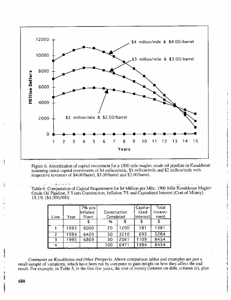
Table 5 and Figure 6 show 15-year projected financial results of a 1500 mile long maglev crude oilpipeline in Kasakhstan, starting with 250,000 barrels per day' in the first year and increasing in 5 years to1,000,000 barrels per day', financed and taxed under conditions generally found in the U.S.A., i.e., 70%debt, 30% equity, interest on debt 13%, return on equity 20%, (combined cost of money 15.1%), costescalation 5%, income taxes dO%, tax depreciation 10%, property taxes 1%. Table 5 shows the resultassuming that original construction cost was $4 million per mile and revenues at $4.00 per barrel (plusannual escalation). Figure 6 shows three curves, $4, $3 and $2 million per mile original construction costlevels with respective $4.00, $3.00 and $2.00 per barrel revenue levels ('also plus annual escalation).

Table 5. 15 Year Projected Financial Results of 1500 Mile, 1,000,000 Barrels per Day MaglevCrude Oil Pipeline in Kasakhstan at Original Cost Estimate of $4 Million per Mile and Revenues at$4.00 per Barrel ($1,000,000)

LineProp.

Year Revenue Opr. Exp Taxes(a) (b) (c)

1 1996

2 1997

3 19984 1999

5 2000

6 2001

7 2002

8 2003

9 2004

10 2005

11 2006

12 2007

13 2008

14 200915 2010

Tax

Deprec.(d)

Intereston Debt

(e)

IncomeTax

(f)

Returnon

Equity(g)

Debt

Repay-ments

(h)

Remain.Debt

Balance

(i)423 131 90 845 769 0 507 -872 9327

665 137 92 845 849 0 560 -748 10075932 144 94 845 917 0 604 -586 10661

1223 151 96 845 970 0 640 -378 11039

1798 159 98 845 1005 0 662 139 10900

2157 167 100 845 992 21 654 485 10415

2265 175 102 845 948 78 625 587 9828

2378 184 104 845 894 140 590 702 9126

2497 193 106 845 830 209 548 830 8295

2622 203 108 845 755 284 498 973 7322

2753 213 110 845 666 367 439 1133 61892'891 224 112 845 563 458 371 1310 4879

3035 235 114 0 444 897 293 1170 3710

3187 247 117 0 338 994 223 1358 23511413346 259 119 0 15681102214 783

Table 6 shows how the initially estimated capital requirement of $4 million/mile times 1500 miles = $6billion increases bv inflation and capitalized interest during three years' of construction to $8.454 billion.This amount plus first year loss of $0.872 billion (Table 5, line (I), column (h)) equals the $9.327 billion inTable 5, line (1), column (i).

679i

kU

J

O,Im

I:

12000

10000

8OOO

6OOO

4000

2000

0

$2 million/mile & $2.00/barrel

$4 million/mile & $4.00/barrel

million/mile & $3.00/barrel

1 2 3 4 5 6 7 8 9 10 11 12 13 14 15

Years

" : : -_ :: .... 7 Z

Figure 6. Amortization of capital invcstment ?or a lS00 mile maglev crude oil pipeline in Kasakhstan :assuming initial capital investments of $4 million/mile, $3 million/mile and $2 rnillion/mile withrespective revenues of $4.00/barrel, $3.00/barrel and $2.00/barrel.

-Table 6. Computation of Capital Requirement for $4 Million per Mile, 1500 Mile Kasakhstan MaglevCrude Oil Pipeline, 3 Years Construction, Inflation 7% and Capitalized Interest (Cost of Money)

is. 1% ($1,ooo,ooo)

Line

1

2

34

Year

1993

7% p/aInflated

Plant$

6000

Capita-lized

Interest

$

ConstructionCompleted% $

20 1200

50 3210

30 2061

100 6471

181

TotalInvest-

ment

1381

1994 6420 693 5284

1995 6869 1109 84541918"4 - 8454

Comnwnts on Kasakhstan and Other Prospects. Above comparison tables and examples are just asmall sample of variations, which have been run by computer to gain insight on how they affect the endresult. For example, in Table 5, in the first few years, the cost of money (interest on debt, column (e), plus

680

i,|

i

return on equity, column (g)) is more than 10 times as large as operating, expense, column (b). Hence,keeping capital costs down is much more important than keeping operating expenses down. Figure 6 showsthe amortization curves rising in the first few years due to the losses as calculated in Table 5, column (h),lines (1) to (4). If oil field prcx.tuction could be started at full capacity in the first year of pipeline operations,billions of dollars could be saved. However, in Alaska, it took five years before they had enough oil for the

pipeline to run at full capacity. As to the cost of money, if one could finance a project with just one percentless in interest, for example cut interest on debt from 13% to 12% for the $4 million/mile curve in Figure 6,it would mean construction cost savings of $100 million and 15 year operations savings of $1.5 billion.

GREAT OPPORTUNITY FOR HIGH TECH AND MONEY MAKING

The above described basic components of the maglev crude oil pipeline, the permanent magnets, thelinear induction motors and the container string with its folding function, are all pretty well straight forward

and relatively simple and reliable technologies. There are opportunities for improvements in magnets,materials and container design, but the most challenging tasks lie in the field of maintenance (especially

leakage prevention), lateral guidance, controls and failure prevention.

L#war hsduction Motors (IYMs) and Controls. As stated in Figure 2 above, LIMs may be spaced asmuch as 100 miles apart at unmanned stations. However, the LIM shown in Figure 2 is only suitable fordriving the system at high speed. For start up, intermediate speeds and reverse braking, several otherspecially designed LIMs are to be located next to the high speed LIMs. Additionally, for every type of LIMneeded in operations throughout the speed range and reverse braking there will need to be one or more LIMsof equal size on standby. Motors may need to either be c_x_led heavily during start up or switched on and offin rotation. As an example, there might be five heavy thrust start up LIMs at each station that get thecontainers up to a speed of 5 mph. Each would take a turn and run for 20% of the time, and be off 80% ofthe time for cooling. There would also be a danger of overheating the containers. They must not stay toolong over an active LIM.

To get a comparison of the magnitude, the largest movements of weight on land are unit trains for coal,ore or grain. They often have 100 cars, each carrying 100 tons for a total of 10,000 tons per train. A 100mile long section of a maglev pipeline, having a capacity of 1,000,000 barrels per day, would weigh alsoabout 10,000 tons (not counting the empty return line). So, the starting LIMs for each 100 mile section ofmaglev pipeline would have to exert a propulsion effort comparable to that of the (usually) eight locomotivesof a unit train. However, for a 1500 mile Kasakhstan line it would require an effort equivalent to 120locomotives. While this looks like an enormous physical task, the cost savings with magIev as calculatedabove would also be enormous.

Power Supply to IJM Stations. The Alaska pipeline has a mi_ of energy sources for pumping. NearPrudhoe Bay several pump stations receive natural gas from the oil field. Further along, oil from the line isdropped off, refined and then used for jet engine powered pumping. Also some power is obtained fromprivate utilities. A maglev pipeline would probably also lc_k at the best available but reliable source. If noother sources are available, one or more small power generating stations would be built and power linesstrung along the same posts that carry the pipeline, see Figure 4.

Surge Suppressors. Common at hydroelectric power stations are surge towers for the purpose ofpreventing structural damage from sudden shut downs of the turbines following a power failure. Thetremendous kinetic energy of the approaching water is dissipated by rising up in these surge towers andoverflowing. The long stream of maglev pipeline containers has a similar problem and a similar solution.Along the line at intervals are longitudinal surge suppressor stations. These are kx:ations where thecontainers are, for a short distance, forced by an upper and lower track to partially fold, similar to what is

shown in Figure 3, above. However, unlike the rigidly fixed lower track in Figure 3, the lower track in asurge suppressor station is vertically movable so that it can absorb longitudinal surges that may run through

681

the containers. These stations also serve to compensate for longitudinal temperature expansions andcontractions of the containers.

l_ztteral Guidance of Containers. Some 150 years ago, a transportation scientist by the name ofEarnshaw, after experimenting with permanent magnets in repulsion, declared that 'it is impossible tosuspend vehicles with permanent magncts in repulsion without secondary help', which is today known asEarnshaw's Theorem (ref. 4). While Einstein was able to refute Newton, nobody has yet been able to refuteEarnshaw. Hence, we are stuck with the need for lateral guidance to ensure that the containers stay abovetheir magnetic track and not fall off to the sidcs. Several methods of lateral guidance controls have beensatisfactorily tested. They are items (I) to (3) below. However, items (4) and (5) below are being l_x_ked at

as possible future "_ternatives.

(1) Self-adjusting, self-lubricating commercially available plastic sliders attached in pairs to each side

of each container. The sliders follow polished stainless steel lined channels which are attached to the insideof the conduits, see left half of Figure "71Thesliders are peri0d_caJiy renewedl Unlike cieciro magneiic : i: :

systems described below, this latcral guide meth_l is fully operational throughout the speed range and needsno backup support system in case of power failure or at slow spee&:

(2) Shown in the right half of Figure 7 are electro magnets attached in pairs to each side of eachcontainer, which are controlled by a gap sensor. A gap separates the electro magnets from dua!channelswith steel inserts. Power for the electro magnets may be generated off the permanent track magnets thatsuspend the containers (Figure 1). This system requires backup support in Case of power failure andpossibly also at low speed.

(3) Electro magnets with steel rails as in (2) above, except they are switched around. The electromagnets _e stationary and the steel rails are attached to the moving containers. Power for the electromagnets can be either generated off the permanent magnet track or supplied by power lines that run along thepipeline. This system also requires backup support in case of powcr failure.

Steel liner Plastic sliderOil filled containers Electro magnet

Conduits Steel insert

Channels

682

Mechanical " EJectro magnetic

Figure 7. Typic.,fl choices of lateral guidance systems, mechanical or electro magnetic. For clarity,

levitation magnets and LIMs are not shown.

=

=

=

7.

_2

(4) New magnetic suspension technology achievements as reported in NASA's 1991 first InternationalSymposium on Magnetic Suspension Technology (ref. 7). These include practical applications of replacingfriction bearings of rotary machinery with non-contact electro magnetic bearings. It seems feasible to havethe container string of the maglev pipeline take the place of a rotating shaft of similar diameter and likewisehave it controlled to remain contactless in the center while moving along at great speed. This system would

also need backup support in case of power failure.

(5) A possible break-through in technology. Magnetic suspension by means of permanent magnets inrepulsion is somewhat similar to riding a bicycle. At no speed and at low speed both have a strong tendencyto fall over. However, at high speed it is nearly impossible to tip over with a bicycle. Remember, the kidshouting: 'Look Ma, no hands'? A bike becomes more and more self-steering as speed increases. By thesame token, it should be possible to develop a kind of magnetic rudder that automatically steers the maglevcontainers through the center of the conduits when at high speed. Backup guidance support would be need at

low speed, but power failures might not affect it.

Quality Controls and Failure Protection. If a light bulb goes out in a life buoy' that marks a shippingchannel, an automatic mechanism rotates another bulb in its place. If the second one goes, a third one comes

up. New aircraft engines are tested numerous times. After each test, they are taken apart, checked and X-rayed until the probability of future failure has become extremely low. These are two examples of how toprevent-disasters of major proportions. Both aircraft and shipping disasters, in addition to loss of life, canrun into millions, even billions of dollars.

The above Kasakhstan pipeline proposal would car D' 1,000,000 barrels of oil per day; that meansabout a million dollars' worth of oil every hour. Figure 6 shows how running at less than full capacity in the

first five years has increased the indebtedness instead of decreasing it. It is obvious that any delay,breakdown or shut down would run into big financial losses. Hence, life buoy style, aircraft style and even

better quality controls must be incorporated in design, operations and maintenance of a maglev crude oil

pipeline, which might be the subject of a future paper.

CONCLUSION

It is obvious that, as easily accessible sources of fossil fuel become depleted, a more economic landtransportation mode needs to be developed. The 800 mile long Alaska (pumped) pipeline is an example ofunsatisfactory and uneconomical present day pumping technology. Other remotely' located oil fields lieuntapped as they wait for advancements in trans[:x_rtation technology. Magnetic levitation is that newadvancement in technology. A maglev crude oil pipeline could go very long distances and still be highlyprofitable in the hands of private enterprise. In the Alaska case, $10 million per day ($73 billion over 20years) might have been saved, had the maglev technology been available and had it been used. Twice as longas the Alaska pipeline, a maglev crude oil pipeline from Tengiz in Kasakhstan to the Black Sea wascalculated above to be also financially feasible.

The major components of the maglev crude oil pipeline are either mechanical or basic electrical innature, which may need little further refinement. However, there are several areas of design and operationswhich need to be addressed and refined. To name a few, operational safety, quality control, failure

prevention, start up procedure, shutdown procedure, lightning strikes, leakage, spills, earthquakes, groundshifting, temperature extremes, vandalism, guerilla attacks, etc. It is not going to be a simple project.However, the future looks bright fc_r maglev pipelines. There is an immediate need to also transport c_.xal,grain and ore more economically'. Further into the future, it may some day be economically feasible totransl:x_rt water by, maglev pipeline from the north to arid lands in Arizona, New Mexico and Texas and turnthem into lush green agricultural lands to supplement the world ik×)d supply.

683

REFERENCES

i. Official Stenographers Retx-_r_, Federal Energy Regulatory C6mmissi0n, Docked No: iSCy'2-3-000,Technical Conference, Amerada Hess Pipeline Company, June 3, 1992. ,:

2. Knolle, E. G.; Knolle Magnetrans, A Magnetically Levitated Train System,, NASA CP 3152,August 19-23, 1991, pp. 907-918.

" 7

Strnat, K. J., Rare-Earth Permanent Magnets: Two Decades of New Magnetic Materials, ASM,Paper No. 8617-005, 1986: - _:_=;:-::_

z

4. Laithwaite, E. R.; Transport Without Wheels, Westview Press, Boulder, Colorado, pp. 304-317,1977.

5. Nonaka, S. and Higuchi, T. ; Design Strategy of Single-Sided Linear Induction Motors for

Propu!slion of Vehicles, IEEE Trans., Cat, No. 87CH2443-0, pp. 1-11, 1987.

6. Knolle, E. G.; Articulated Train System, U.S. Patent No.3,320,903, Re. 26673, 1969.

7. lnteruational Symposium oil Magnetic Suspension Technology, NASA Conference Publication

3152, Langley Research Center, 1991.

w

[

2

E

684

Appendix

Attendees

Byong AhnCharles Stark Draper Laboratory555 Technology SquareM.S. O3

Cambridge, MA 02139617-258-2832

Paul Allaire

University of VirginiaDept. Mech, Aerosp, NuclearThornton Hall, McCormick RoadCharlottesville, VA 22901804-924-3292

Willard W. Anderson

NASA Langley Research Center

Mail Stop 479Hampton, VA 23681-0001804-864-1718

Tyler M. AndersonBoeing Defense & Space GroupP.O. Box 3999MS 182-24

Seattle, WA 98124206-773-2291

Bill G. AsburyLockheed Engineering and Sciences144 Research Drive

Hampton, VA 23666804-766-9600

Clayton C. BearRevolve Technologies, Inc.1240 - 700 - 9 Avenue, S.W.

Calgary, Alberta T2P 3V4 CANADA403-261-5338

Brij B. BhargavaAshman Consulting ServicesP.O. Box 3189

Santa Barbara, CA 93130-3189805-964-2104

Barry BlairWaukesha BearingsP.O. Box 1616

Waukesha, WI 53187414-547-3381

685

Karl BodenKFA-IGVPF-1913W-5170Julich D-52425 GERMANY49-2461-614604

Dr. Hans J. BornemannKernforschugszentrum KarlsruheINFP, P. O. Box 364076021 Karlsruhe GERMANY49-7247-82-6389

Lyle A. BranaganPacific Gas & Electric

3400 Crow Canyon RoadSan Ramon, CA 94583510-866-5735

Colin P. Britcher

Old Dominion University

Dept. of Aerospace EngineeringNorfolk, VA 23529-0247804-683-4916

Thomas C. Britton

Lockheed Engr. and Science Co.24 West Taylor RoadMail Stop 161Hampton, VA 23681-0001804-864-6619

Stephen ChapmanMagnetic Bearings, Inc.524i Valleypark DriveRoanoke, VA 24019703-563-4936

David E. Cox

NASA Langley Research CenterMail Stop 161Hampton, VA 23681-0001804-864-8149

Harold R. Davis

The University of British ColumbiaDepartment of Physics6224 Agricultural RoadVancouver, B.C. V6T 1Z1 CANADA604-822-2961

686

Dr. Horst Ecker

Technical University ViennaInst. fr. Machine Dyn. & MeasuremtWiedner Hauptstr. 8-10/303Vienna A-1040 AUSTRIA43-222-58801-5567

James H. Eggleston46th TEST Group/TKE1 E21 EST Track RoadHolloman AFB, NM 88330-7847505-679-2941

James B. Fischer

Electron Energy Corporation3307 E. Romelle Avenue

Orange, CA 92669714-538-7328

Martha L. Fisher-Votava

Sundstrand Aerospace4747 Harrison AvenueRockford, IL 61125-7002815-394-2729

Karl FlueckigerCharles Stark Draper LaboratoryMail Stop 3H555 Technology SquareCambridge, MA 02139617-258-3850

Lucas E. Foster

Old Dominion University

Dept. of Aerospace EngineeringNorfolk, VA 23529-0247804-683-3720

Giancarlo GentaPolitecnico di Torino

Mechanics DepartmentC. Duca degli Abruzzi24-10120 Torino, ITALY39-11-5646901

Michael J. GoodyerThe University of Southampton

Dept. of Aero. and Astro.Southampton SO9 5NH ENGLAND44-703-592374

687

Henry GuckelWl Cntr for Applied MicroelectronicsElectrical & Computer Engineering1415 Johnson Drive

Madison, WI 53706-1691608-263-4723

Ram GurumoorthyGECRD1 River Road

Bldg. K-l, Rm. 4C20Schenectady, NY 12065518-387-6657

Roy D. HamptonUniversity of VirginiaROMAC Labs, Mech & Aero EngrgThornton Hall, McCormick RoadCharlottesville, VA 22901804-924-3767

Lee M. HartwellRKR Associates1607 Southwood Blvd.

Arlington, TX 76013817-795-7124

Robin Harvey

Hughes Research Labs3011 Malibu Cyn RoadMalibu, CA 90265310-317-5236

Toshiro HiguchiUniversity of TokyoKSP East 405, 3-2-1 SakadoTakatsu-kuKawasaki-shi 213 JAPAN81-44-819-2048

Kwok W. Hui

Dresser Rand CompanyP. O. Box 560Olean, NY 14760716-375-3328

688

John Y. HungAuburn UniversityDept of Electrical Engineering200 Broun Hall

Auburn University, AL 36849-5201205-844-1813

James D. HurleyMechanical Technology Inc.968 Albany Shaker Rd.Latham, NY 12110518-785-2177

A. Dean JacotBoeing Aerospace CompanyP. O. Box 3999MS 82-24Seattle, WA 98124206-773-8629

Graham JonesTechnology Insights10240 Sorrento Valley RoadSuite 320San Diego, CA 92121619-455-9080

Brian R. JonesLawrence Livermore Nat. LaboratoryP. O. Box 808L630Livermore, CA 94550415-423-3058

Swarn KalsiGrumman CorporationM/S B29-25Bethpage, NY 11714516-356-9624

Yoichi KanemitsuEBARA Research Company, LTD.MSR Dept., Electro-physics Lab.2-1, fujisawa 4-chomeFujisawa-shi 251 JAPAN81-466-83-7640

Claude R. KecklerNASA Langley Research CenterMail Stop 479Hampton, VA 23681-0001804-864-1718

Allan J. KelleyThe University of TokyoKanagawa Academy of Sci. & Tech.KSP E. 405, 3-2-1 SakadoTakatsu-ku Kawasaki 213 JAPAN81-44-819-2093

689

Yoshida KinjiroKyushu UniversityDept. of Electrical Engineering6-chome 10-1, Hakozaki Higashi-kuFukuoka 812 JAPAN092-641-1101, X5307

Ronald L. Klein

West Virginia UniversityDept of Electrical/Computer Eng.P.O. Box 6101

Morgantown, WV 26506-6101304-293-3998

Josiah D. Knight _ _ Ernst G. Knolle

Duke University Knolle MagnetransDept. of Mechanical Engineering 2691 Sean Cou_ ...... _ _

Box 90300 ' S. San Francisco, CA 94080 •Durham, NC 27708-0300 415-871-9816 " =919-660-5337 :

S. KohlerSandia National Laboratories

Albuquerque, NM 87185

John C. KroegerHoneywell Satellite Sys.Box 52199

Phoenix, AZ 2199 ,602-561-3175

690

Dr. Alexander V. KuzinUNC-Charlotte

Precision Engineering LabCharlotte, NC 28223704-547-4324

Jaynarayan H. LalaCharles Stark Draper Lab., Inc.555 Technology SquareMS 73

Cambridge, MA 02139617-258-2235

Kyong B. LimNASA Langley Research CenterMail Stop 161Hampton, VA 23681-0001804-864-4342

Chin E. LinNational Cheng Kung Univ.Inst. of Aeronautics and AstronauticsTainan 70101 TAIWAN886-6-274-1820

Reinhard F. LuerkenThyssen Henschel America, Inc.2730 Wilshire BoulevardSuite 500Santa Monica, CA 90403310-828-9768

James P. LyonsGE Corporate R&DP.O. Box 8, EP-116Schenectady, NY 12309518-387-5015

Sam MallicoatMicrofield Graphics, Inc.9825 SW Sunshine CourtBeaverton, OR 97005503-626-9393

Oliver MarrouxAerospatiale66 Route de VerneuilLes Mureaux, 78133 FRANCE33-1-34922822

David B. MartinNorthrop ATDCN214/XA8900 E. Washington BoulevardPico Rivera, CA 90660310-942-3362

Osami MatsushitaThe National Defense AcademyDept. of Mechanical Engineering603 Kandatsu-machiKanegawa JAPAN 23981-468-41-3810, X2326

691

Wally McLellanMagnetic Bearings, inc.5241 Valleypark DriveRoanoke, VA 24019703-563-5936

Chase K. McMichael

Texas Center for SuperconductivityUniversity of Houston4800 Calhoun

Houston, TX 77204-5506713-743-8254

James L. MilnerNational Maglev Initiative, USDOT400 7th Street, S.W.Room 5106, RDV-1

Washington, DC 20590202-366-0515

R. Mark Nelms

Auburn UniversityDept. of Electrical Engineering200 Broun Hall

Auburn, AL 36849205-844-1830

Steven A. NolanRockwell International

Rocketdyne Division, Mail Stop IA326633 Canoga Avenue, P.O. Box 7922Canoga Park, CA 92309-7922818-718-4430

Alan B. Palazzolo

Texas A&M UniversityMechanical EngineeringCollege Station, TX 77843-3123409-845-5280

Da-Chen PangUniversity of MarylandDepartment of Mech. Engg.College Park, MD 20742301-405-787

Richard F. PostLawrence Livermore National Lab

P. O. Box 808, L-644Livermore, CA 94551510-422-9853

_= 692

A. K. PradeepGeneral Electric CR&DP. O. Box 8

Schenectady, NY 1230151 8-387-6588

Mark A. Preston

General Electric Corporate R&DP. O. Box 8, Building EPRoom 116

Schenectady, NY 1230151 8-387-5588

Douglas B. PriceNASA Langley Research CenterMail Stop 161Hampton, VA 23681-0001804-864-6605

Michael Proise

Grumman CorporationMail Stop B29-25Bethpage, NY 11714516-346-2100

James C. RipleAllied Signal28626 Vista Madera

Rancho Palos Verdes, CA 90732310-512-4586

James D. RobergeSatCon Technology Corporation12 Emily StreetCambridge, MA 02139617-661-0540, X272

Robert SalterXerad1526 14th Street

Santa Monica, CA 90404

Philippe Save De BeaurecueilSouthern California Edison CompanyGO3 Third Floor2131 Walnut Grove Avenue

Rosemead, CA 91770818-302-8272

693

Dr. Hideo Sawada

National Aerospace Laboratory7-44-1 Jindaijihigashi-machiChofu-shi

Tokyo 182 JAPAN81-422-47-5911

J. Schmeid

Sulzer Escher Wyss Ltd.Abteilung T733PostfachCH-8023 Zurich SWITZERLAND

41-1-278-3118

Richard Schoeller, Jr.Naval Surface Warfare Center

3A Leggett CircleAnnapolis, MD 21402-5067410-267-2651

Dr. Roland Y. SiegwartMecos Traxler AGGutstrasse 38Winterthur S CH-8400 SWITZERLAND

41-52-2329288

Devendra K. Sood

GE Aircraft Engines1000 Western AvenueM.D.-170MW

Lynn, MA 0191061 7-594-3061

Albert F. StoraceGeneral Electric Aircraft Engines

1 Neumann WayMail Drop A334Cincinnati, OH 45215513-774-5047

Claus C. ThiesenTechnical Services Company10510 N.E. 45th Street

Kirkland, WA 98033206-822-2609

R. TortiSatCon Technology Corp.

12 Emily StreetCambridge, MA 02139-4507617-661-0540

694

Michael Urednicek

REVOLVE Technologies Inc.1240 Western Canadian Place700 Ninth Avenue S.W.

Calgary, Alberta T2P 3V4 CANADA403-261-5329

Jim Walker

Walker Technology17561 Hada Drive

San Diego, CA 92127619-487-4788

Michael H. Walmer

Electron Energy Corporation924 Links AvenueLandisville, PA 17538717-898-2294

Mark E. Williams

University of NC at CharlottePrecision Engineering DepartmentCharlotte, NC 28223704-547-3145

695

Form Approved

REPORT DOCUMENTATION PAGE OMBNo 0704-018B

Public reporting burden for this coIlection of information is estimated to average I hour per response, including the time for reviewing instructions, searching existing data sources,gathering and maintaining the data needed, and completing and reviewing the collection of _n[ormatior_ Send comments regarding this burden estimate or any other aspect of thiscolIect_on of information, including suggestions for reducing this burden, toWashlngton Headquarters Services, Directorate for information Operations and Reports. 1215 JeffersonDavis Highway, Suite 1204, Arlington, VA 22202-4302, and to the Office of Management and Budget, Paperwork Reduction Project (0704-01B8). Washington, DC 20503.

|. AGENCY USE ONLY(Leave blank) 2. REPORT DATE 3. REPORT TYPE AND DATES COVERED

May 1994 Conference Publication

:4. TITLE AND SUBTITLE

Second International Symposium on Magnetic Suspension Technology

6. AUTHOR(S)

Nelson J. Groom and Colin P. Britcher, Editors

7. PERFORMING ORGANIZATION NAME(S) AND ADDRESS(ES)

NASA Langley Research CenterHampton, VA 23681-0001

9. SPONSORING/MONITORING AGENCY NAME(S) AND ADDRESS(ES)

National Aeronautics and Space AdministrationWashington, DC 20546-0001

5. FUNDING NUMBERS

WU 233-03-01-01

8. PERFORMING ORGANIZATION

REPORT NUMBER

_17_9

10. SPONSORING/MONITORING

AGENCY REPORT NUMBER

NASA CP-3247Part 2

11. SUPPLEMENTARY NOTES

Nelson J. Groom: Langley Research Center, Hampton, VA; Colin P. Britcher:Norfolk, VA

Old Dominion University,

12a. DISTRIBUTION/AVAILABILITY STATEMENT 12b. DISTRIBUTION CODE

Unclassified-Unlimited

Subject Category 18

13. ABSTRACT (Maximum 200 words)

In order to examine the state of technology of all areas of magnetic suspension and to review related recent devel-opments in sensors and controls approaches, superconducting magnet technology, and design/implementationpractices, the 2nd International Symposium on Magnetic Suspension Technology was held at the Wcstin Hotelin Seattle, Washington on August 11-13, 1993.

The symposium included 18 technical sessions in which 44 papers were presented. The technical sessionscovered the areas of bearings, bearing modelling, controls, vibration isolation, micromachines, superconductiv-ity, wind tunnel magnetic suspension systems, magnetically levitated trains (MAGLEV), rotating machineryand energy storage, and applications. A list of attendees appears at the end of the document.

14. SUBJECT TERMS

Magnetic bearings; Magnetic suspension; Large gap magnetic suspension; Smallgap magnetic suspension; Sensors; Superconducting magnetic suspension systems;Control systems

17. SECURITY CLASSIFICATION 18. SECURITY CLASSIFICATION 19. SECURITY CLASSIFICATION

OF REPORT OF THIS PAGE OF ABSTRACT

Unclassified Unclassified Unclassified

_ISN 7540-01-280-5500

15. NUMBER OF PAGES

278

16. PRICE CODE

A1320. LIMITATION

OF ABSTRACT

;tandard Form 2cJS(Rev. 2-8g)Prescribed by ANSI Std. Z39-18298-102