Maglev Train Propulsion System

Catherine Pavlov

1 Abstract

This project was an experiment on the feasibility of superconductor-based maglev trains. Two classmates, Kyle Tessier-Lavigne and Michael Stern, and I worked in conjunction to produce a magnetic track, levitating train car, and propulsion system. This paper focuses on my part of the project, the propulsion system. The propulsion system is similar to a linear motor, with a row of solenoids attracting and repulsing a magnet atop the train car. The propulsion system increases the speed of the train, but is not yet strong enough to move the train car all the way around the track from a stationary position. The magnetic fields from the electromagnets had a field of 8x10-4 T, which exerted a force of 5.4x10-3 N on the train, accelerating it at 0.09936 m/s/s.

2 Introduction

This project is a study of the real-world feasibility of maglev trains as a transportation system. As many countries move to make themselves “greener,” one of the biggest questions is, “How can we be more efficient?” Because transportation uses up such a large amount of energy, this is one of the first places to turn when looking for ways to be more environmentally friendly. Maglev trains could very well be the transportation of the future, as they have virtually no friction, making them incredibly efficient and silent. There are several types of maglev trains: those made from permanent magnets, those made from electromagnets, and those made from superconductors. As trains employing permanent magnets and electromagnets are more difficult to build, this project utilizes superconductors.

This paper was written for Dr. James Dann’s Applied ScienceResearch class in the spring of 2011.

Getting something to levitate is relatively easy and has been done many times. Once a superconductor is lowered to its critical temperature, the point at which the material becomes superconducting, it exhibits the Meissner Effect, [6] in which the superconductor excludes magnetic fields, causing it to “float” above magnets. While the levitation of a superconductor is easily shown, using superconductors for transportation is somewhat trickier, as they must stay cooler longer and need some horizontal propulsion system. Another setback in the real-world feasibility of superconductor maglev trains is the cost of superconductors, which are currently very expensive. While one can’t predict the future, it is very likely the cost of superconductors will eventually go down, as more is learned about them and their seemingly magical properties.

High-speed rail systems have already been implemented all over the world, from France to Japan. Maglev trains have not yet become a common public phenomenon, mainly because thus far their advantages over normal high-speed rail are often not enough to justify building trains and tracks from scratch. [7] If more research is done into the top speed and efficiency of maglev trains, there is the possibility of their more widespread application in real-world use. Information from this type of research could also be applied to normal high-speed trains. Aerodynamic design from both maglev and high-speed trains could even be applied to slower moving trains, such as subways, to help increase the efficiency of transportation systems that are not ready for total reform.

While maglev trains are not yet feasible for widespread commercial application, a few pioneering trains have already been built, such as the electromagnetic train in Shanghai, [8] from which others can learn by example, to create a new era of efficient transportation.

This project focused mainly on the propulsion system, an area not typically focused on, at least in small-scale demonstrations. Many model maglev trains don’t address propulsion at all, or use mechanical systems to accelerate the train. [9] The goal of this project is to create an effective, no-contact propulsion system that has the capability to be reversed, for stopping and multidirectional movement.

58 Catherine Pavlov

Over the course of this project I wanted to learn more about superconductors and electromagnetic propulsion systems, especially with regards to green energy. I also wished to learn more about electronics and make more complicated circuits. The opportunity to work with superconductors, which are not entirely understood yet, was also amazing, as it is really interesting to study current science, rather than only repeating past experiments.

3 A Brief History of Maglev Trains and Superconductivity

Superconductivity was discovered in 1911 by Dutch physicist H. Kammerlingh Onnes, who observed the phenomenon after cooling mercury to 3 K with liquid helium. [17] It was first discovered in pure metals, which must be cooled to extremely low temperatures. There are thirty metals that exhibit superconductivity at very low temperatures. These superconductors make up a class called Type I superconductors. [1] The superconductor used in this experiment was a YBCO superconductor, which is Type II. The BCS theory of superconductivity, which is detailed later in this paper, was developed by John Bardeen, Leon Cooper, and Robert Schrieffer. Bardeen, Cooper, and Schrieffer won the Nobel Prize in 1972 for their work in describing superconductivity. [2] Maglev trains are not a new concept. Thomas Bachelet and Robert Goddard both came up with ideas for maglev in the early twentieth century, but had no way to actually create them. In 1934, Hermann Kemper received a patent for magnetically levitated trains, but maglev was not practical for transport until some decades later. In 1966, a maglev system consisting of superconducting magnets that induced a current in a conductor was proposed by James Powell and Gordon Danby. [3] This concept was explored further with working scale models built that functioned at speeds of 97 km/hr. This type of levitation is called Inductrack. There are two other main kinds of levitation in maglev trains: EMS and EDS. In EMS, or an electromagnetic system, the levitation force comes from attracting electromagnets on the train that lift it off of the track. In EDS, or an electrodynamic system, electromagnets in the guideway repulse the train, levitating it above the track. [4] Because the train does not touch the track, there is very

THE MENLO ROUNDTABLE 59

low resistance to motion, allowing maglev trains to be highly efficient. This efficiency makes maglev a viable substitution for transport in the future. [3] Currently, there is a high-temperature superconducting maglev train in Shanghai, China. There is still work to be done on developing maglev trains, as they are costly to build and the linear electromagnetic propulsion systems usually used are not highly efficient. [5] However, despite the current costs of building maglev trains, they may prove to be relatively inexpensive in the future due to increased ease of creating superconductors as technology develops. More importantly, any superconducting maglev would need very minimal repair and upkeep, as the absence of moving parts means that no hardware on the train would wear out. Maglev may have a way to go, but it has a very promising future.

4 Theory and Results

The maglev trains in this project levitate though a phenomenon called the Meissner effect, which occurs in superconductors. Certain materials achieve superconductivity when lowered to extremely low temperatures. The superconductors used in this experiment are YBCO superconductors, which are made of a ceramic-based compound that enters a superconducting state at a relatively high temperature. [6]

Superconductivity and the Meissner effect are relatively new phenomenon, and so there is still much to be understood about them. When a superconductor passes its critical temperature, the point at which it becomes superconducting, it has no resistance to current, so that a current in the material will continue indefinitely. Superconductors also exclude magnetic fields, which is the cause of the Meissner effect. This is explained in part by Faraday’s law, which states that a conductor in a changing magnetic field produces a current to create a field opposing the change. The currents created in a superconductor exclude external fields from all but the very surface of a superconductor. However, Faraday’s law does not explain how superconductors can levitate magnets placed above them before cooling them to a superconductive state, or how they bounce back up after being pushed towards the surface of a superconductor. [10]

60 Catherine Pavlov

While there are many competing theories as to how superconductivity works, the most widespread one is the BCS theory, named for its creators Bardeen, Cooper, and Schrieffer. [11] In BCS theory, electrons act together in pairs, called Cooper pairs. When Cooper pairs form, an electron is attracted to positive ions in the crystal lattice, pulling them together. This increased concentration of charge then attracts another electron of opposite spin. [12] The two spins effectively cancel, exempting the Cooper pair from the Pauli exclusion principle and allowing the electrons to move as one without resistance to their movement.

The superconductors used in this project are YBCO superconductors, which have the chemical formula YBa2Cu3O7. YBCO superconductors generally have a critical temperature of around 90 K. [13] Using a kit provided by Colorado Superconductor, Inc., I attempted to verify this through a short experiment.

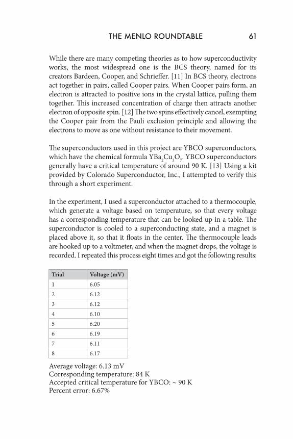
In the experiment, I used a superconductor attached to a thermocouple, which generate a voltage based on temperature, so that every voltage has a corresponding temperature that can be looked up in a table. The superconductor is cooled to a superconducting state, and a magnet is placed above it, so that it floats in the center. The thermocouple leads are hooked up to a voltmeter, and when the magnet drops, the voltage is recorded. I repeated this process eight times and got the following results:

Trial Voltage (mV)1 6.052 6.123 6.124 6.105 6.206 6.197 6.118 6.17

Average voltage: 6.13 mV Corresponding temperature: 84 KAccepted critical temperature for YBCO: ~ 90 KPercent error: 6.67%

THE MENLO ROUNDTABLE 61

While superconductors often transition from a superconducting state to a non-superconducting state over a range of a few degrees, the results from the experiment were fairly different from the accepted value. It is unlikely the thermocouple is to blame for this error, as the one used in this experiment is a Type T [6] thermocouple, which typically is accurate within about 1° C. [14] This would not account for the error in the measurement of critical temperature. It is possible that the superconductor somehow changed, either by reacting with the environment or because of realignments of the internal crystal structure due to use.

The superconductor used in this experiment was meant only for demonstrations, so I am using a much larger YBCO superconductor for the train. If possible, I will determine the critical temperature of the larger superconductor through a similar experiment, to see if the results are comparable.

The propulsion system is based on permanent magnets and electromagnets, with permanent magnets attached to the top of the train and solenoids integrated into a no-contact propulsion system that sits above the train tracks. The propulsion system is based on the fact that the magnetic flux through a loop of wire is proportional to the current in the wire. By reversing the current, the polarity of the field is reversed, and by altering the magnitude, the strength of the field is changed. Because the forces between the magnets and the solenoids in this system are proportional to the magnetic fields involved, altering the current in the solenoid, and by extension changing its magnetic field, should theoretically control the speed of the train. Additionally, by reversing the direction of current once the train is already in motion, the train can be slowed or brought to a stop.

The magnetic field in the center of the solenoid can be calculated by using the following equation: [15]

B = μ0NI

62 Catherine Pavlov

B represents the magnetic field, I the current through the loop, N the number of turns, and μ0 the constant for the permeability for free space, 4π x10-7 N/A2. While the number of turns is not exactly known, it can be estimated. By measuring the resistance of a piece of wire of known length identical to that used in the solenoid, and comparing it to the resistance of the solenoid, the length of wire used can be found. The average circumference of a loop in the solenoid can be found from the radius, and by dividing the length of the wire by the average circumference an approximate number of loops can be found, and the magnetic field inside the solenoid can be calculated. Adding a core to the solenoid amplifies the field. As the centers of the solenoids in this project are comprised mainly of iron, the magnetic field is multiplied by about 200. [16]

I took the resistance of a 5 m length of wire, and measured it as 1.21 Ω. The resistance of the multimeter was 0.13 Ω, giving a total resistance of 1.08 Ω for 5 m of wire, or 0.22 Ω/m. The resistance of one of the solenoids was 26.28 Ω, when the resistance of the multimeter was subtracted. This gave for a total length of 125 m. The diameter of the solenoid was 3.5 cm, giving each loop an average circumference of 5.5 cm, or 0.055 m. This leads to each solenoid having approximately 455 loops.

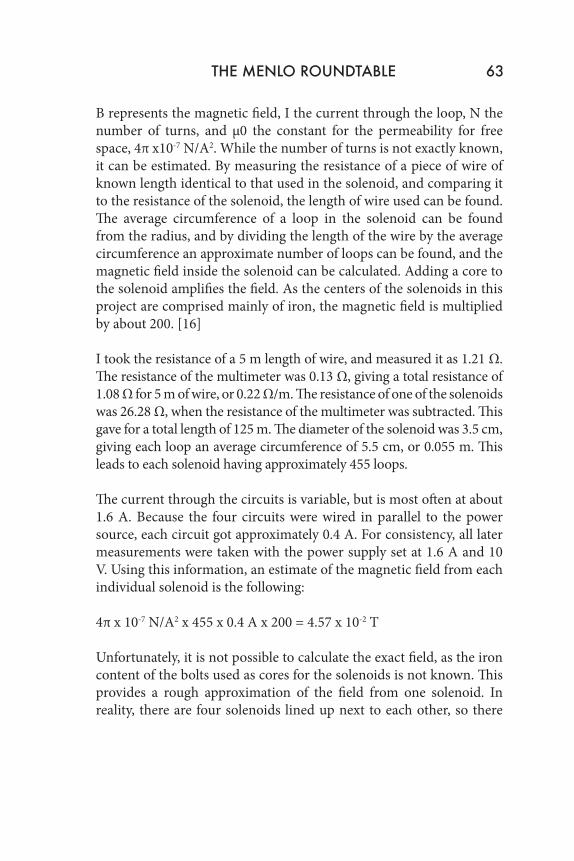
The current through the circuits is variable, but is most often at about 1.6 A. Because the four circuits were wired in parallel to the power source, each circuit got approximately 0.4 A. For consistency, all later measurements were taken with the power supply set at 1.6 A and 10 V. Using this information, an estimate of the magnetic field from each individual solenoid is the following:

4π x 10-7 N/A2 x 455 x 0.4 A x 200 = 4.57 x 10-2 T

Unfortunately, it is not possible to calculate the exact field, as the iron content of the bolts used as cores for the solenoids is not known. This provides a rough approximation of the field from one solenoid. In reality, there are four solenoids lined up next to each other, so there

THE MENLO ROUNDTABLE 63

is also some interference from the fields from other electromagnets, adding another difficulty in calculating the exact field. It is, however, possible to measure the magnetic field. I measured the magnetic fields of both the electromagnets and the magnet atop the train car using a Hall effect sensor. Because the top of the train is 3.5 cm below the electromagnets, I measured the fields from 3.5 cm away. I measured the field of the electromagnet to be 0.80 mT, or 8 x 10-4 T. The field from the permanent magnet was considerably stronger, at 4.3 x 10-3 T. The measured field was much lower (57 times) than the calculated field, probably because of several reasons: it was measured at a distance, the iron content of the core in the calculations was probably overestimated, and other electromagnets probably had interfering fields that affected the measurement.

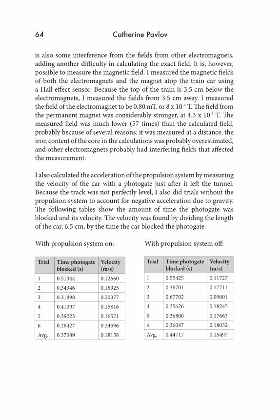
I also calculated the acceleration of the propulsion system by measuring the velocity of the car with a photogate just after it left the tunnel. Because the track was not perfectly level, I also did trials without the propulsion system to account for negative acceleration due to gravity. The following tables show the amount of time the photogate was blocked and its velocity. The velocity was found by dividing the length of the car, 6.5 cm, by the time the car blocked the photogate. With propulsion system on: With propulsion system off:

Trial Time photogate blocked (s)

Velocity (m/s)

1 0.51344 0.126602 0.34346 0.189253 0.31898 0.203774 0.41097 0.158165 0.39223 0.165716 0.26427 0.24596Avg. 0.37389 0.18158

64 Catherine Pavlov

Trial Time photogate blocked (s)

Velocity (m/s)

1 0.55425 0.117272 0.36701 0.177113 0.67702 0.096014 0.35626 0.182455 0.36800 0.176636 0.36047 0.18032Avg. 0.44717 0.15497

These measurements were taken with the voltage of the propulsion system set at 10 V, and the current at about 1.6 A. The distance traveled for the propulsion tests was 30.5 cm, and the distance traveled for the gravity tests was 26.5 cm.

To find the acceleration, I used the following equation:

(v2) = (v02) + 2aΔx

Because the initial velocity was 0, this gives the following:

a = (v2)/(2Δx)

Using the average velocities for the trials with the propulsion system, this gives an acceleration of

(0.18158 m/s)2/(2 x 0.305 m) = 0.05405 m/s/s

and a gravitational acceleration of

(0.15497 m/s)2/(2 x 0.265 m) = 0.04531 m/s/s

As the trial with the propulsion system was facing uphill, the acceleration due to gravity should be added to the net acceleration with the propulsion system, giving an acceleration of 0.09936 m/s/s.

Using the mass and velocity of the train, I calculated the kinetic energy at the end of the propulsion system. Because work, or change in energy, is the applied force times the distance it is applied over, I used the kinetic energy and the distance to find the average force exerted on the car. The mass of the train was 100 grams, and the velocity used was the average velocity, or 0.18158 m/s. Below are the calculations:

W=Fd=ΔE=1/2mv2

F=(mv2)/2dF=(0.1 kg x (0.18158 m/s)2)/(2 x .305 m)= 5.4 x 10-3 N

THE MENLO ROUNDTABLE 65

In summary: the propulsion system had an electromagnetic field of 8 x 10-4 T and applied a force of 5.4 x 10-3 N to the train car, which had a mass of 0.1 kg, and accelerated it at 0.09936 m/s/s.

5 Drawings and Diagrams

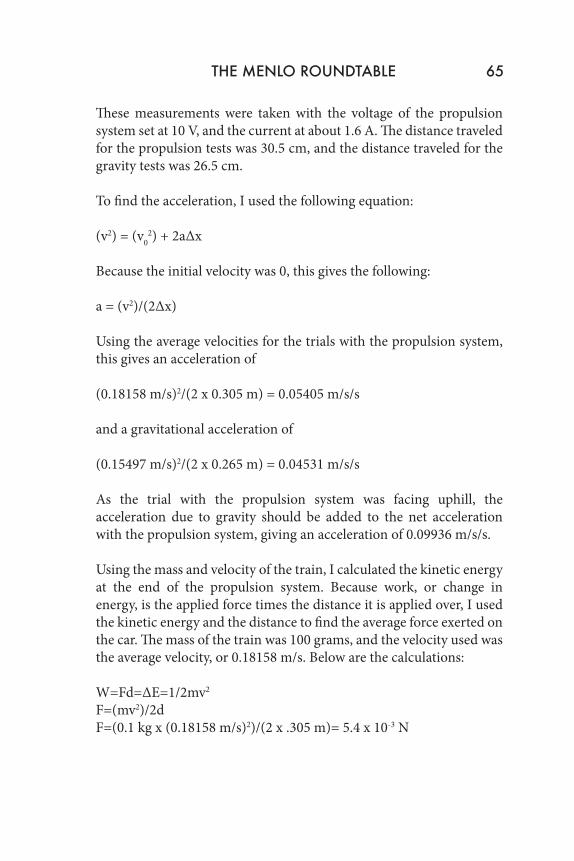
Figure 1: Overall drawing of the experimental setup, with magnetic track and propulsion system in large box. The cylinders within the box show the solenoids that repel the magnets on the train.

66 Catherine Pavlov

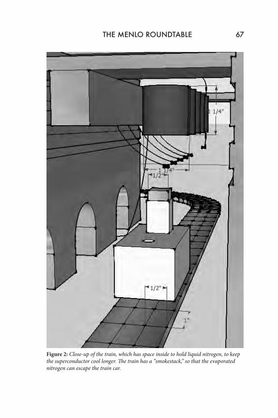
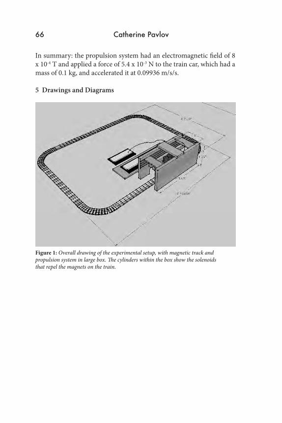
Figure 2: Close-up of the train, which has space inside to hold liquid nitrogen, to keep the superconductor cool longer. The train has a “smokestack,” so that the evaporated nitrogen can escape the train car.

THE MENLO ROUNDTABLE 67

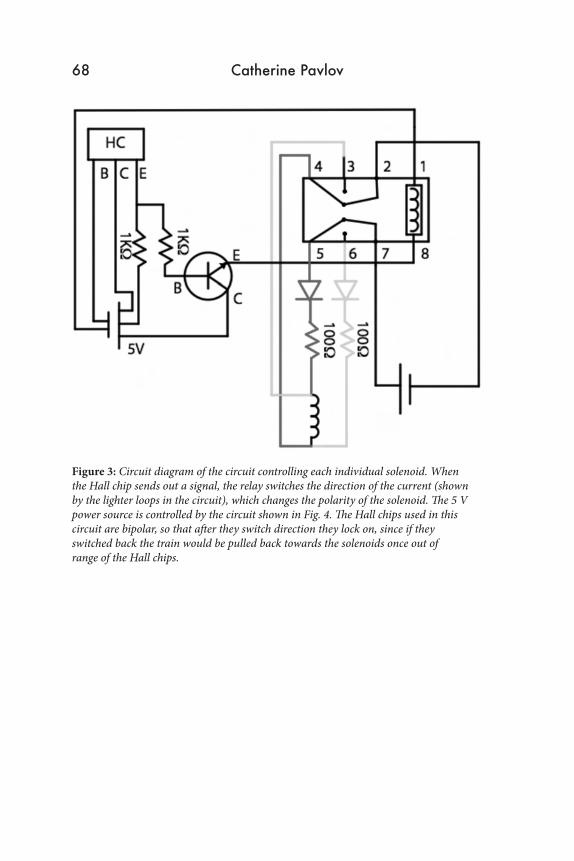
Figure 3: Circuit diagram of the circuit controlling each individual solenoid. When the Hall chip sends out a signal, the relay switches the direction of the current (shown by the lighter loops in the circuit), which changes the polarity of the solenoid. The 5 V power source is controlled by the circuit shown in Fig. 4. The Hall chips used in this circuit are bipolar, so that after they switch direction they lock on, since if they switched back the train would be pulled back towards the solenoids once out of range of the Hall chips.

68 Catherine Pavlov

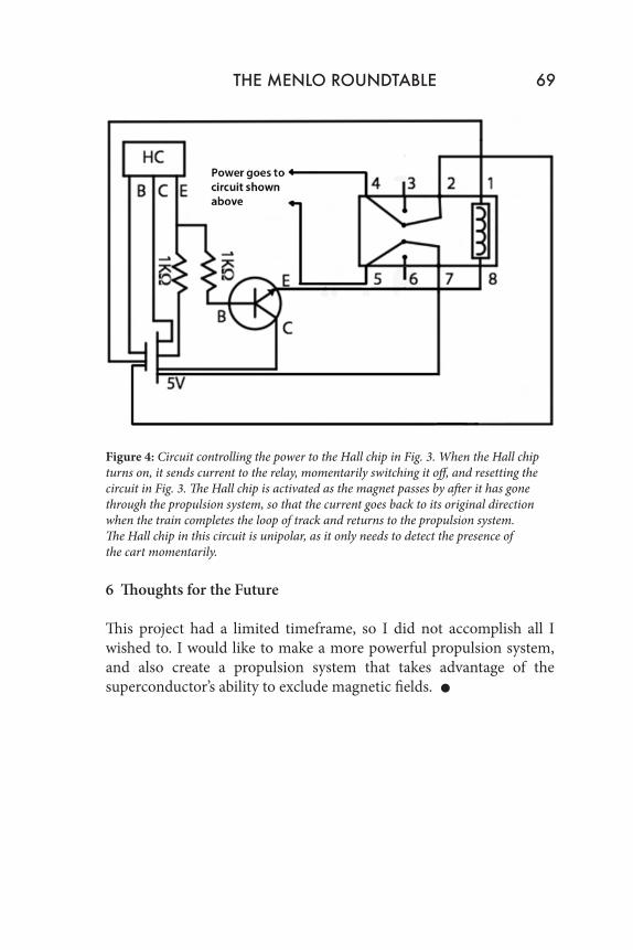
Figure 4: Circuit controlling the power to the Hall chip in Fig. 3. When the Hall chip turns on, it sends current to the relay, momentarily switching it off, and resetting the circuit in Fig. 3. The Hall chip is activated as the magnet passes by after it has gone through the propulsion system, so that the current goes back to its original direction when the train completes the loop of track and returns to the propulsion system. The Hall chip in this circuit is unipolar, as it only needs to detect the presence of the cart momentarily.

6 Thoughts for the Future

This project had a limited timeframe, so I did not accomplish all I wished to. I would like to make a more powerful propulsion system, and also create a propulsion system that takes advantage of the superconductor’s ability to exclude magnetic fields.

THE MENLO ROUNDTABLE 69

7 Bibliography

[1] Carl Nave, Superconductivity, http://hyperphysics.phy-astr.gsu.edu/hbase/solids/scond.html (2010).

[2] Carl Nave, BCS Theory of Superconductivity, http://hyperphysics.phy-astr.gsu.edu/hbase/solids/bcs.html (2010).

[3] “The History of Maglev,” Mag Lev Builders, http://www.pulaki.com/sites/maglev/history.htm.

[4] “Introduction to MagLev Monorail,” The Monorail Society. http://www.monorails.org/tmspages/TPMagIntro.html.

[5] Jiasu Wang, Suyu Wang, and Jun Zheng, “Recent Development of High Temperature Superconducting Maglev Trains in China,” IEEE/CSC & ESAS European Superconductivity News Forum, No. 7. (January 2009).

[6] Experiment Guide for Superconductor Demonstrations, Colorado Superconductor (2004).

[7] Tony Eastham, “High Speed Rail: Another Golden Age?” Scientific American. (September 1995).

[8] Shanghai Maglev Train, www.smtdc.com/en/ (2005).

[9] http://www.youtube.com/watch?v=6lmtbLu5nxw&feature=related (2009).

[10] Carl Nave, Perfect Diamegnetism, http://hyperphysics.phy-astr.gsu.edu/hbase/hframe.html.

[11] Paul A. Tipler, “Superconductivity,” Physics for Scientists and Engineers (Extended Version) (1991).

70 Catherine Pavlov

[12] Hugh D. Young and Roger A. Freedman, “Superconductivity,” University Physics with Modern Physics, 11th Edition (2004).

[13] The Kelvin Scale of Temperature, http://www.users.qwest.net/~csconductor/ (2001).

[14] Thermocouples, http://www.omega.com/prodinfo/thermocouples.html.

[15] Paul A. Tipler, “Sources of the Magnetic Field,” Physics for Scientists and Engineers (Extended Version) (1991).

[16] Carl Nave, Relative Permeability, http://hyperphysics.phy-astr.gsu.edu/hbase/solids/ferro.html#c5 (2010).

[17] Davide Castelvecchi, “Absolute Hero: Heike Onnes’s Discovery of Superconductors Turns 100,” Scientific American, http://www.scientificamerican.com/ (2011).

THE MENLO ROUNDTABLE 71