MAGNETIC COUPLING BETWEEN DC TACHOMETER AND

MAGNETIC COUPLING BETWEEN DC TACHOMETER AND MOTOR AND ITS EFFECT ON MOTION CONTROL IN THE PRESENCE OF

SHAFT COMPLIANCE

by

Shorya Awtar

A Thesis Submitted to the Graduate

Faculty of Rensselaer Polytechnic Institute

In Partial Fulfillment of the

Requirements for the Degree of

MASTER OF SCIENCE

Approved:

_____________________________

Professor Kevin C. Craig Thesis Advisor

Rensselaer Polytechnic Institute Troy, New York

August 2000

ii

TABLE OF CONTENTS

LIST OF FIGURES……………………………………………………………………..iv

LIST OF TABLES……………………………………………………………………..viii

ACKNOWLEDGEMENTS……………………………………………...………..……ix

ABSTRACT……………………………………………………….……………………...x

1. INTRODUTION……………………………………...……………………………..1

2. EXPERIMENTAL SET-UP………………………………………………………..3

2.1 System Description……………………………………………………...3

2.2 Component Specification………………………………………………..4

3. CONVENTIONAL TACHOMETER MODEL AND ITS DEFICIENCY…..….7

4. MODELING OF D.C. MACHINES………………….…………………………..12

4.1 D.C. Motor……………………………………………………………..13

4.2 D.C. Tachometer……………………………………………………….17

4.3 Coupled D.C. Motor-Tachometer System……………………………..20

5. EXPERIMENTAL VERIFICATION OF THE PROPOSED MODEL……….30

5.1 Discussions on the proposed Tachometer model………………………33

6. TYPICAL APPLICATION: MOTION CONTROL IN PRESENCE OF

SHAFT COMPLIANCE…………………………………………………………..35

7. CONTROL SYSTEM DESIGN……………………………….………………….42

7.1 Introduction…………………………………………………………….42

7.2 Colocated and Noncolocated Control………………………………….44

7.2.1 Two-mass single-spring system…………………….……44

7.2.2 Open-loop characteristics: Physical Significance of

poles and zeros…………………………………………...47

iii

7.2.3 Close-loop characteristics: Stability Analysis…………...51

7.2.4 Multiple mass systems………………………….………..66

7.3 Tachometer-Motor-Load System………………………………………70

8. CONCLUDING REMARKS AND FUTURE WORK…………………………..83

REFERENCES……………………………………………………………...…………..85

iv

LIST OF FIGURES

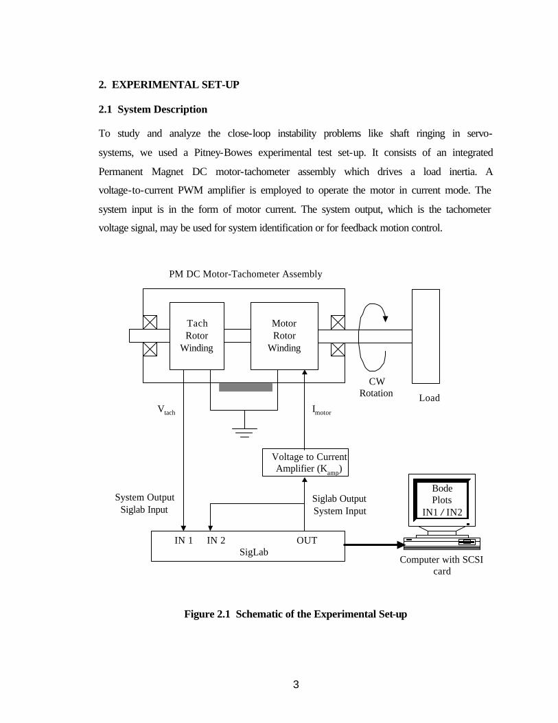
Fig. 2.1 Schematic of Experimental Set-up……………………………………………..3

Fig. 3.1 Physical model of the motor-tachometer system………………………………7

Fig. 3.2 Effect of damping on the zeros and poles of a system…………………………8

Fig. 3.3 Comparison of the analytically-predicted and experimentally-obtained

frequency response plots for the motor-tachometer system….…...…………..10

Fig. 4.1 Electrical circuit diagram for a D.C. Motor…………………………………..14

Fig. 4.2 Physical model for a D.C. motor……………………………………………...14

Fig. 4.3 Interaction between two magnetic fields……………………………………...15

Fig. 4.4 Physical model for a D.C. tachometer………………………….……………..18

Fig. 4.5(a) Angular orientations of the motor and tachometer permanent magnets…...21

Fig. 4.5(b) Motor and Tachometer fields………………………………………………21

Fig. 4.6(a) Magnetic Fields present in the Tachometer………………………………..22

Fig. 4.6(b) Magnetic Fields present in the Motor…….………………………………..23

Fig. 4.7 Transformer effect between the motor armature coil and the tachometer

armature coil…………………………………………………………………..25

Fig. 5.1 Comparison of the analytically-predicted and experimentally-obtained

frequency response plots for the motor-tachometer system….…...…………..31

Fig. 6.1 Motor-tachometer-load system…………………………………………...…...36

Fig. 6.2 Physical Model of the motor-tachometer-load system………………………..37

Fig. 6.3 Vtach/Vin: Comparison of experimental frequency response and predicted

frequency response using conventional model……………………………….39

Fig. 6.3 Vtach/Vin: Comparison of experimental frequency response and predicted

frequency response using proposed model…………………………..……….39

Fig. 7.1 Two-mass single-spring system………………………………………………44

v

Fig. 7.2 Bode plot for x1 / Fin transfer function……………………………………..….45

Fig. 7.3 Bode plot for x2 / Fin transfer function……………………………………...…46

Fig. 7.4 System frequency response when excitation force is applied on mass-1……..49

Fig. 7.5 Bode plot for x2 / x1 transfer function…………………………………………50

Fig. 7.6(a) Root-locus for the rigid body case ( 21

s)………………………………….52

Fig. 7.6(b) Bode plots for the rigid body case ( 21

s)………………………………….52

Fig. 7.7(a) Root-locus for the rigid body case with lead compensation ( 2

2ss+

)………53

Fig. 7.7(b) Bode plot for the rigid body case with lead compensation ( 2

2ss+

)………..54

Fig. 7.8(a) Root-locus plot for the uncompensated colocated system (22

122 2

1( )s z

s s p++

)…55

Fig 7.8(b) Bode plots for the uncompensated colocated system (22

122 2

1( )s z

s s p++

)……...56

Fig 7.9(a) Root-locus plot for the compensated colocated system:

22

122 2

1

( 2)( )s z

ss s p

++

+…………………………………………………………57

Fig. 7.9(b) Root-locus plot for the compensated colocated system:

22

122 2

1

( 2)( )s z

ss s p

++

+…………………………………………………………58

Fig. 7.10(a) Root-locus for the uncompensated noncolocated system ( 22 21

1( )s s p+

)….59

Fig. 7.10(b) Bode plots for the uncompensated noncolocated system ( 22 21

1( )s s p+

)….59

Fig. 7.11(a) Root-locus plot for the lead compensated noncolocated system:

vi

( 22 21

1( 2)

( )s

s s p+

+)……………………………………………………….60

Fig. 7.11(b) Bode plots for the lead compensated noncolocated system:

( 22 21

1( 2)

( )s

s s p+

+)……………………………………………………….61

Fig. 7.12(a) Root-locus plot for the notch compensated noncolocated system…………62

Fig. 7.12(b) Bode plots for the notch compensated noncolocated system………………63

Fig. 7.13(a) Root-locus for the notch compensated noncolocated system in the

presence of pole-zero flipping……………………………………………..64

Fig. 7.13(b) Bode plots for the notch compensated noncolocated system in the

presence of pole-zero flipping……………………………………………..65

Fig. 7.14 Multiple-mass multiple-spring system……………………………………..…66

Fig. 7.15 Four-mass three-spring system………………………………………………..67

Fig. 7.16(a) Pole-zero flipping in a noncolocated system……………………………....68

Fig. 7.16(b) Pole-zero flipping in a noncolocated system……………………………....69

Fig. 7.17 Physical System and Physical Model………………………………………...70

Fig. 7.17(a) t

mTθ

: Root-locus for the tachometer-motor-load mechanical system………72

Fig. 7.18 Root locus for (a) Uncompensated system (b) Lead compensated system…...73

Fig 7.19 Bode Plots for the system with lead compensation…………………………...74

Fig 7.20 Block-diagram based representation of the open-loop tachometer-motor-load

mechanical and electrical system……………………………………………..76

Fig. 7.21 The tachometer-motor-load electromechanical system………………………76

Fig. 7.22 Close-loop block diagram of the tachometer-motor-load electromechanical

system…77

vii

Fig. 7.23(a) Root-locus plot (b) Bode plots for the uncompensated system…………...79

Fig. 7.24(a) Root-locus plot for the lead compensated tachometer-motor-load

electromechanical system……………………………………………...….80


electromechanical system……………………………………………...….81

viii

LIST OF TABLES

Table 2.1 Specifications of the Electro-craft DC Motor Tachometer assembly………..4

Table 2.2 Specifications of the Advanced Motion Controls PWM amplifier…………..5

Table 2.3 Specifications of the Power Supply…………………………………………..5

Table 3.1 List of symbols used in Section 3 ……………………………………………7

Table 4.1 List of symbols used in Section 4.1…………………………………………13



Table 5.1 List of symbols used in Section 5...…………………………………………30

Table 6.1 List of symbols used in Section 6...…………………………………………35

Table 6.2 Comparison of experimentally observed and theoretically predicted

(using the proposed model) zero and pole frequencies.……………………40

ix

ACKNOWLEDGEMENTS

I am thankful to my thesis advisor Professor Kevin C. Craig for his guidance and support.

I also wish to express my thanks to my colleagues, Celal Tufekci and Jeongmin Lee for

their help during the course of this research.

x

ABSTRACT

This thesis presents an accurate tachometer model that takes into account the effect of

magnetic coupling in a DC motor-tachometer assembly. Magnetic coupling arises due to

the presence of mutual inductance between the tachometer winding and the motor

winding (a weak transformer effect). This effect is modeled and experimentally verified.

Tachometer feedback is widely used for servo-control of DC motors. The presence of

compliant components in the drive system, e.g., shafts, belts, couplings etc. may lead to

close-loop instability which manifests itself in the form of high frequency ringing. To be

able to predict and eliminate these resonance related problems, it is essential to have an

accurate tachometer model. This thesis points out the inadequacies of the conventional

tachometer model, which treats the DC tachometer as a ‘gain’ completely neglecting any

associated dynamics. It is shown that conventional models fail to predict the experimental

system dynamics response for high frequencies. The exact tachometer model identified in

this research is incorporated in the modeling of a system that has multiple flexible

elements, and is used for parameter identification and feedback motion control.

Predictions using this new model are found to be in excellent agreement with

experimental results. The effect of the tachometer dynamics on controller design is

discussed in the context of system poles and zeros.

Key words: DC Tachometer model, DC motor motion control, shaft flexibility, sensor

dynamics, system poles and zeros, shaft ringing.

1

1. INTRODUTION

Closed-loop servo control of a DC motor-load system is a very common industrial and

research application. Very often DC tachometers are used to provide velocity feedback

for motion control [3, 4, 5]. In the presence of flexibility in the system, e.g., a compliant

motor-load shaft or a flexible coupling, this exercise in servo control becomes quite

involved since finite shaft stiffness introduces resonance and shaft ringing. These are

highly undesirable effects that can be eliminated by means of appropriate controller

design. To be able to model, predict, and eliminate these high-frequency resonance

problems, it is essential to have an accurate model for the entire system including the

sensor.

There are papers in the literature that discuss the control system design for systems with

mechanical flexibilities [4, 6, 8, 10]. There are also extensive discussions on colocated

and non-colocated control in the literature. The problem is explained in terms of poles

and zeros of the system [6, 7, 8, 9, 10]. All these discussions assume that a ‘perfect’

position or velocity signal is available for feedback and that sensor dynamics is

negligible. Such an assumption might be acceptable for routine applications, but is not

useful for high-performance applications. It is emphasized in this thesis that an accurate

model for the sensor dynamics is necessary and should be incorporated in the control

system design.

In the case of DC motor position and/or velocity control using tachometer feedback, the

conventional tachometer model [1, 2, 3] is adequate for less demanding motion control

exercises, but is ineffective for rendering high-speed and high-precision motion control.

In fact, when this model was used to predict the frequency response of a system with

multiple shaft flexibilities, it yielded erroneous results that did not agree with the

experimental measurements. This led to an investigation leading to a more exact and

accurate model for the DC tachometer. A thorough modeling analysis was carried out and

it was found that the mutual inductance between the tachometer and motor windings,

however weak, results in a magnetic coupling term in the expression for the voltage

output of the tachometer. This effect is quantitatively studied and derived in this thesis,

2

and an enhanced tachometer model is obtained using the basic principles of

electromagnetism. This model is then used to analyze a DC tachometer-motor-load

system with multiple flexible elements. It is found that the new analytical predictions are

in excellent agreement with the experimental measurements.

The consequence of this tachometer dynamics on the over-all system response is

explained. It is seen that the tachometer dynamics influences the system transfer function

in a way that is system dependent. This shall become clear in the following sections. We

find that the tachometer dynamics contributes some additional zeros to the overall system

transfer function. The number of these additional zeros depends on the system itself. The

location of these zeros in the s-plane is determined by the relative orientation of the

tachometer stator field with respect to the motor stator field. Having experimentally

confirmed the model, we subsequently incorporate it in the feedback control design for

DC motor motion control, which is the final objective of this entire exercise. The

significance and implication of these additional zeros in terms of controller design is

discussed in detail.

This thesis is organized in the following manner. Section 2 describes the experimental

setup used for this research. Section 3 investigates the inconsistency presented by

convention DC tachometer model. It is explained why the conventional model is

inadequate for high performance servo-control design. A detailed description of

Permanent Magnet DC machines is presented in Section 4. This covers the existing

model and the derivation of a more accurate model. The experimental validation of the

new model obtained in Section 4 is presented in Section 5. Section 6 describes the

application of this model to an actual system with multiple flexible elements. Section 7

introduces the control design problems and issues related to it. A detailed discussion on

colocated and noncolocated system is presented. These concepts are then extended to the

tachometer-motor-load system, and the influence of tachometer dynamics on the control

system design is explained. Finally, compensator designs for eliminating close-loop

instability problems in the tachometer-motor-load system are discussed. Section 8

summarizes this research and lists the conclusions from this work.

3

2. EXPERIMENTAL SET-UP

2.1 System Description

To study and analyze the close-loop instability problems like shaft ringing in servo-

systems, we used a Pitney-Bowes experimental test set-up. It consists of an integrated

Permanent Magnet DC motor-tachometer assembly which drives a load inertia. A

voltage-to-current PWM amplifier is employed to operate the motor in current mode. The

system input is in the form of motor current. The system output, which is the tachometer

voltage signal, may be used for system identification or for feedback motion control.

Figure 2.1 Schematic of the Experimental Set-up

System OutputSiglab Input

IN 1 IN 2 OUT SigLab

TachRotor

Winding

MotorRotor

Winding

Voltage to CurrentAmplifier (Kamp)

Computer with SCSIcard

BodePlots

IN1 / IN2

PM DC Motor-Tachometer Assembly

Load

Siglab OutputSystem Input

CWRotation

Vtach Imotor

4

The first phase of experimentation is performed to obtain frequency response plots for the

above-described system, which is an exercise in system identification. For this purpose,

we use a DSP tool, SigLab. SigLab sends a sine sweep over a user-specified frequency

range as the system input in the form of a voltage signal to the current amplifier. At the

same time it also collects the system output, which is the tachometer voltage in this case.

Based on this input-output data, SigLab constructs the frequency response plots for the

system. A schematic of this set-up is shown in Figure 2.1.

Motor polarity is chosen such that a positive motor current (Im) leads to a CW rotation of

the rotor. Tachometer polarity is chosen such that a CW rotation of the rotor produces a

positive tachometer voltage (Vtach).

2.2 Component Specifications

1) DC Motor-Tachometer Assembly.

The motor and tachometer used for this set-up is a Permanent Magnet Brushed DC

Motor-Tach assembly, Model No. 0288-32-003 from Electro-Craft Servo Products.

Table 2.1 Specifications of the Electro-Craft 0288-32-003 DC Motor with Tachometer

Motor Characteristics Units Values

Rated Voltage (DC) volts 60

Rated Current (RMS) amps 4

Pulsed Current amps 29

Continuous Stall Torque oz-in 50

Maximum Rated Speed RPM 6000

Back EMF Constant volts-/krpm 8.7

Torque Constant oz-in/amp 11.8

Terminal Resistance ohms 1.0

Rotor Inductance mH 3.3

5

Viscous Damping Coefficient oz-in/krpm 11.3

Rotor Inertia (including Tach) oz-in-sec2 0.0078

Static Friction Torque lb-in 0.19

Tachometer Voltage Constant volts/krpm 14

2) Power Amplifier

The power amplifier used in this system is the Advanced Motion Controls PWM

servo-amplifier, Model 25A8.

Table 2.2 Specifications of the Advanced Motion Controls Model 25A8 PWM Amplifier

Power Amplifier Characteristics Values

DC Supply Voltage 20-80 V

Maximum Continuous Current ± 12.5 A

Minimum Load Inductance 200 µH

Switching Frequency 22 Khz ± 15%

Bandwidth 2.5 KHz

Input Reference Signal ± 15 V maximum

Tachometer Signal ± 60 V maximum

3) Power Supply

A DC power supply is used to drive the system.

Table 2.3 Specifications of CSI/SPECO Model PSR-4/24 Power Supply

Power Supply Characteristics Values

Supply voltage +24 Volts

Maximum Continuous Current 4 amps

Maximum Peak Current 7 amps

6

4) DSP Tool

The DSP used for this experiment is the SigLab 20-42 hardware/software tool from

DSP Technology Inc. This DSP tool has the following features:

• DC to 20 kHz frequency range

• Fully alias-protected two or four-channel data acquisition system in one small

enclosure

• Expandable from two to sixteen channels

• Ready to use Windows-based measurement and analysis software, coded in

MATLAB

• On board real time signal processing provides 90dB alias protection and frequency

translation (zoom)

• Integrated multifunction signal generation

Further information is available on the company website: http://www.dspt.com

7

3. CONVENTIONAL D.C. TACHOMETER MODEL AND ITS DEFICIENCIES

Table 3.1 List of symbols used in this section

Variable/Parameter Symbol Value

Motor angular position θm -

Tachometer angular position θ t -

Motor armature inertia Jm 43.77e-6 kg-m2

Tachometer armature inertia Jt 11.35e-6 kg-m2

Motor-Tach shaft stiffness K 1763 N-m/rad

Motor current im -

Motor torque Tm -

Motor torque constant Kt 8.33e-2 N.m/A

Tachometer voltage Vtach -

Tachometer constant Ktach 0.137 V/(rad/s)

For simplicity, we consider a DC motor-tachometer assembly without any external load

inertia. A shaft of finite stiffness connects the tachometer armature and the motor

armature. A physical model of this assembly with lumped parameters is shown in Figure

3.1.

Figure 3.1 Physical Model of Motor Tachometer assembly

Jt Jm

θt

θm

Tm

K

8

By drawing free-body diagrams for the two inertias Jt and Jm, and applying Newton’s

Second Law, we obtain the following transfer function:

2 2 [ ( )]

t

m t m t m

KT s J J s K J Jθ

=+ +

(3.1)

It is worth-mentioning here that in the derivation of the above transfer function all

frictional losses (Coulomb, viscous and structural) have been neglected. As shall become

clear later in this thesis, the effect of damping terms is not important for the primary

investigation that is being carried out. We are trying to identify the complex conjugate

poles and zeros of the motor-tachometer system that arise due to the mechanical and

electrical characteristics of the system. From a frequency response perspective, damping

does not govern the existence of these poles and zeros. It only tends to reduce their

intensity. This is illustrated in Figure 3.2.

101

-60

-50

-40

-30

-20

-10

0

10

20

30

40

50

Mag

nitu

de (

dB)

frequency

Figure 3.2 Effect of damping on the zeros and poles of a system

Undamped System Response

Damped System Response

9

By presenting this argument, we justify the dropping out of damping terms in our model

for the mechanical system at this stage. In the later part of this thesis though, when we

talk about control system design, the signs of the damping terms become critical in terms

of analyzing the close-loop system stability. At that stage, damping terms shall be

introduced with due justification provided.

We now proceed with the pertinent analysis. Using the conventional DC motor and

tachometer models, commonly found in text-books,

m t m

tach tach t

T K i

V K θ

=

= & (3.2)

to model the motor-tachometer system described in Section 2, and the following overall

system transfer function is obtained,

2

[ ( ) ]amp tach ttach

in t m t m

K K K KVV s J J s K J K

=+ +

(3.3)

This expression indicates the presence of one complex-conjugate pole pair. We get the

frequency response plots for this transfer function using MATLAB. At the same time, we

also obtain the experimental frequency response plots using SigLab as described in

Section 2. The two sets of plots: analytical and experimental, are compared to check how

well the theoretical transfer function predicts the actual system response (Figure 3.3).

10

102

103

-40

-30

-20

-10

0

10

Mag

nitu

de d

B

102

103

-400

-300

-200

-100

0

Frequency (Hz)

Pha

se (d

egre

es)

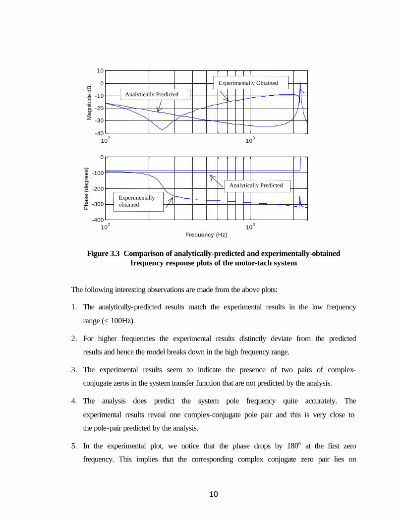
Figure 3.3 Comparison of analytically-predicted and experimentally-obtained frequency response plots of the motor-tach system

The following interesting observations are made from the above plots:

1. The analytically-predicted results match the experimental results in the low frequency

range (< 100Hz).

2. For higher frequencies the experimental results distinctly deviate from the predicted

results and hence the model breaks down in the high frequency range.

3. The experimental results seem to indicate the presence of two pairs of complex-

conjugate zeros in the system transfer function that are not predicted by the analysis.

4. The analysis does predict the system pole frequency quite accurately. The

experimental results reveal one complex-conjugate pole pair and this is very close to

the pole-pair predicted by the analysis.

5. In the experimental plot, we notice that the phase drops by 180o at the first zero

frequency. This implies that the corresponding complex conjugate zero pair lies on

Analytically Predicted

Experimentally Obtained

Experimentally obtained


11

right side of the imaginary axis in the s-plane. This indicates the presence of negative

damping term, which is unusual in a mechanical system.

Evidently, there are many discrepancies noticed in the above comparison that remain

unexplained by the present analytical model for the system. This demands a closer

inspection of the system modeling. Since expression (3.1) is derived by applying

Newton’s Second Law to a widely accepted physical model of a two-mass-one-spring

system, its validity is almost certain. On the other hand, expressions (3.2) represent

textbook models of idealized ‘electromagnetically uncoupled’ motor and tachometer

respectively, which might be an over-simplification. Since their accuracy is questionable,

we proceed to identify any electromagnetic phenomena that might give rise to some

unidentified dynamics.

12

4. MODELING OF D.C. MACHINES

We follow a thorough approach in deriving models for DC machines in order to make

sure that we do not miss the influence of any weak, yet significant electromagnetic effect.

We start from the fundamentals of electromagnetism to study the operation of DC

machines. In the following analysis we have been particularly careful with the signs

associated with various quantities, as any inconsistencies will lead to erroneous

predictions.

In the following discussion, the fundamental laws of electromagnetism will be invoked

frequently. These principles are listed here for the convenience of the reader:

1. Faraday’s Law of Induction: The induced electro motive force, or emf, in a circuit is

equal to the rate at which flux through the circuit changes.

2. Lenz’s Law: As an extension to Faraday’s Law, Lenz’s Law states that the emf

induced will be such that the resulting induced current will oppose the change that

produced it.

3. A combination of the above two laws is expressed in Maxwell’s Third Equation

ddt

εΦ

= − (4.1)

where ε is the induced emf in volts, while phi is magnetic flux in webers. 4. Kirchoff’s Voltage Law (KVL): The algebraic sum of the changes in potential

encountered in a complete traversal of the circuit must be zero.

5. Kirchoff’s Current Law (KCL): The algebraic sum of the currents at any junction in a

circuit must be zero.

13

4.1 D.C. Motor


Variable/Parameter Symbol Units

Permanent Magnet Stator Field of the Motor

Bm wb/m2

Armature Field of the Motor Ba wb/m2

Armature Current in the Motor Ia A

Torque Constant of the Motor Kt_motor N.m/A

Torque generated by the Motor Tm N.m

Flux linkage in Armature Coil due its own Current

Φa webers

Area Vector of Armature Coil (pointing in the same direction as Ba )

A m2

Armature Resistance Ra ohms

Armature Inductance La henry

Number of Armature Coils N -

Input Terminal Voltage to the Motor Vin V

Back emf generated in the Motor Vbackemf V

Angular velocity of the Armature ω rad/s

Back emf Constant Kb_motor V.s/rad

A commonly encountered description for a DC motor is illustrated in the following

circuit, with armature resistance and inductance modeled as lumped quantities.

14

Vb

Ra

La

Vin

Ia

Figure 4.1 Electrical Circuit for a D.C. Motor

Applying KVL to the above circuit leads to the well-known DC motor electrical equation,

_

ain b motor a a a

d IV K L R I

dtω− − = (4.2)

To understand the significance of each term in the above equation, it is desirable to take a

look the derivation of this equation from a much more fundamental level. Consider the

following physical model for a DC motor,

Figure 4.2 Physical Model of a D.C. Motor

N S

Bm (PM Field)Field Axis

Ba (Armature Field)Quadrature Axis

Vin

Ia

15

The permanent magnet stator field (Bm), the direction of which is called the ‘field axis’,

is fixed in space. The armature field (Ba), generated due to the armature current, is

orientated in a direction called the ‘quadrature axis’. Despite the armature rotation, the

quadrature axis retains its orientation in space due to commutation. If we assume a

perfect commutation, then the armature field always remains perpendicular to the stator

field. Repulsion between these two magnetic field vectors produces a clockwise torque

on the rotor that is proportional to the product of Bm and Ba. Bm remains constant and Ba

is linearly dependent on Imotor.

N

S

N S Bm

Ba

Torque on armature

Torque on armature

Figure 4.3 Interaction between two magnetic fields

Hence, the motor torque generated can be expressed as,

m a m mT k B B Bµ= × = ×r r rr

(4.3)

where µ is the magnetic dipole moment resulting from the armature field, and is

proportional to and in the same direction as Ba .

16

(by definition of magnetic dipole moment)

a

a

m a m

m m a

k B

N I A

T N I A B

T N A B I

µ

µ

=

=

⇒ = ×

⇒ =

r rrr

r r (4.4)

Defining the motor torque constant Kt_motor = N A Bm , we arrive at the following simple

expression for motor torque

_ m t motor aT K I= (4.5)

Applying KVL and Ohm’s Law, the governing electrical equation is expressed as,

ain backemf a a

dV V N R I

dtΦ

− − = (4.6)

As is evident from the above equation, there are two effects that oppose Vin: a back emf

that arises due to the armature motion in the stator field Bm, and an induced emf due to

the self-inductance of the armature coil. Both these effects are impeding effects, which is

reflected by the negative sign associated with them (Lenz’s Law). Also, using the

following standard relationships,

_

(generator effect, derieved in Section 4.2)

a a

a a a

backemf b motor

B A

N L IV K ω

Φ = ⋅

Φ ==

rr

(4.7)

we can reduce equation (4.6) to,

_

ain b motor a a a

d IV K L R I

dtω− − = (4.8)

which is the same as equation (4.2). This is the commonly accepted model for an

‘electromagnetically isolated’ D.C. motor. Now we proceed to take a look at the model

for D.C. tachometer.

17

4.2 D.C. Tachometer


Variable/Parameter Symbol Units

Permanent Magnet Stator Field of the Tachometer

Bm wb/m2

Armature Field of the Tach Ba wb/m2

Load Current drawn from the Tach IL A

Torque Constant of the Tach Kt_tach N.m/A

Retarding Torque generated by the Tachometer

Ttach N.m

Flux linkage in the Tach Armature Coil due its own Current

Φa webers

Area Vector of Armature Coil (pointing in the same direction as Ba )

A m2

Armature Resistance Ra ohms

Armature Inductance La henry

Number of Armature Coils N -

Back emf generated in the Tach Vb V

Angular velocity of the Armature ω rad/s

Generator Constant for the Tachometer Kb_tach V.s/rad

Load Resistance RL ohms

18

Figure 4.4 Physical model of a D.C. tachometer

In this case, a CW rotation of the rotor in the presence of the permanent magnet stator

field Bm, produces an emf of Vb across the armature terminals (Faraday’s Law of

Induction: Generator Effect).

Using Faraday’s Law, we know that the emf induced in a conductor of length l, moving

with a velocity v, in a uniform magnetic B field, is given by,

emf l v B= ×rr (4.9)

It can be shown that for a coil rotating in a radially uniform stator field Bm, the induced

emf is given by,

2 ( ) (2 )

b m

b m

b m

V N l r BV N lr BV N A B

ωω

ω

=⇒ =⇒ =

(4.10)

Defining the generator constant (or the tachometer constant) as Kb_tach = N A Bm , leads us

to the following simple relationship for the generator (or tachometer),

_ b b tachV K ω= (4.11)

Bm (PM Field)field Axis

S

Ba (Armature Field)Quadrature Axis

NRLVtach

BrushIL

19

This induced emf causes a current IL in the load resistor, RL. IL also flows through the

tachometer armature, thus producing an armature field Ba along the ‘quadrature axis’.

Once again due to commutation, the orientation of the armature field always remains

perpendicular to the stator field and hence is fixed in space. This current also produces a

retarding torque on the tachometer rotor, which as earlier can be derived to be the

following,

_ tach t tach LT K I= (4.12)

KVL and Ohm’s Law for the above tachometer circuit leads to,

( ) a

b a L Ld

V N R R IdtΦ

− = + (4.13)

Using equations (4.11) and (4.7), this equation further reduces to,

_

( ) Lb tach a a L L

d IK L R R I

dtω − = + (4.14)

The first term on the LHS represents the voltage induced across the armature due to its

motion in the permanent magnet field Bm. Consequently, since the circuit is closed by

means of the external resistance RL, a current IL flows through the circuit. The self-

inductance of the coil tries to oppose the emf that causes IL, hence the negative sign

associated with the second term (Lenz’s Law). The terminal voltage as seen by the

resistor RL is given by,

_

Ltach L L b tach a a L

d IV R I K L R I

dtω= = − − (4.15)

If RL is extremely large, then the current drawn from the tachometer is negligible and the

above expression is reduced to,

_ tach b tachV K ω= (4.16)

This is the model for an ‘electromagnetically isolated’ tachometer that we encounter in

all textbooks and references. Now we proceed to investigate how this changes when a DC

tachometer is placed close to a DC motor.

20

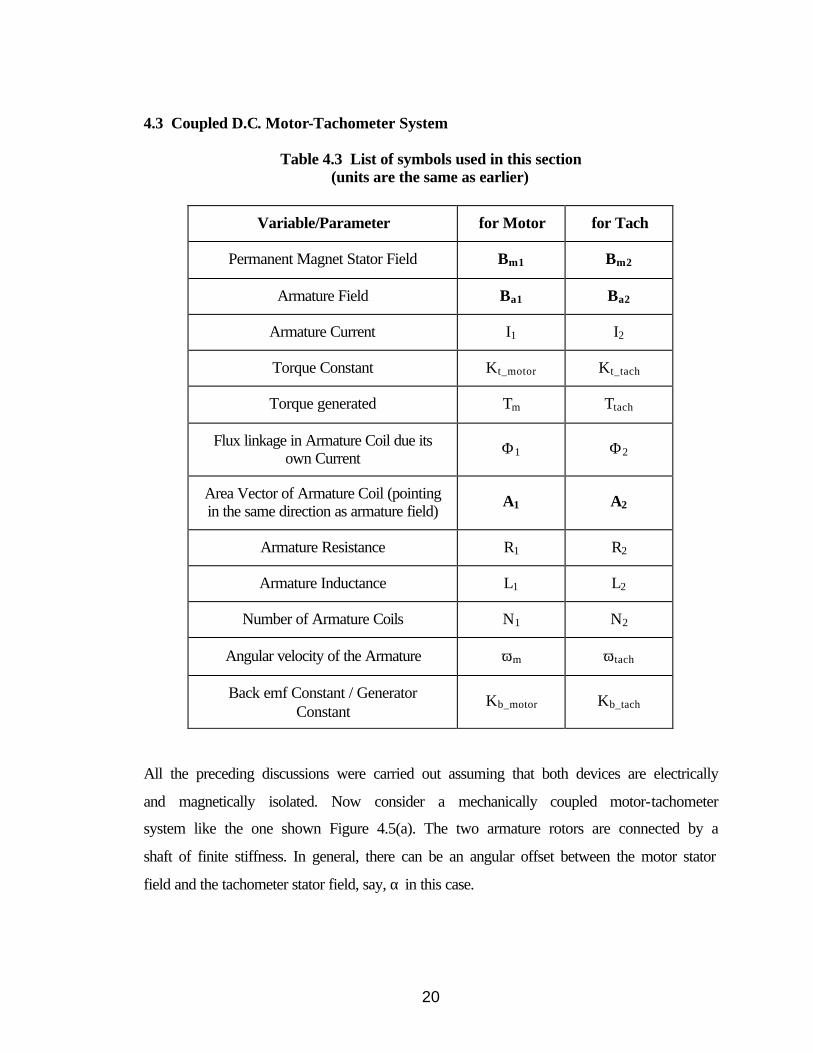
4.3 Coupled D.C. Motor-Tachometer System

Table 4.3 List of symbols used in this section (units are the same as earlier)

Variable/Parameter for Motor for Tach

Permanent Magnet Stator Field Bm1 Bm2

Armature Field Ba1 Ba2

Armature Current I1 I2

Torque Constant Kt_motor Kt_tach

Torque generated Tm Ttach

Flux linkage in Armature Coil due its own Current

Φ1 Φ2

Area Vector of Armature Coil (pointing in the same direction as armature field)

A1 A2

Armature Resistance R1 R2

Armature Inductance L1 L2

Number of Armature Coils N1 N2

Angular velocity of the Armature ωm ωtach

Back emf Constant / Generator Constant

Kb_motor Kb_tach

All the preceding discussions were carried out assuming that both devices are electrically

and magnetically isolated. Now consider a mechanically coupled motor-tachometer

system like the one shown Figure 4.5(a). The two armature rotors are connected by a

shaft of finite stiffness. In general, there can be an angular offset between the motor stator

field and the tachometer stator field, say, α in this case.

21

Figure 4.5 (a) Angular orientations of the Motor and Tachometer permanent magnets (b) Motor and Tachometer Fields

Motor

Tachometer

α

Armature Motor

Armature Tach

CW rotation of the common

rotor

α

Bm1

Bm2

Ba1

Ba2

Ba21

Ba12

MotorFields

TachometerFields

CWRotation

Bm12

Bm21

22

We notice that the armature field of the motor produces a flux linkage in the tachometer

winding and similarly the armature field of the tachometer produces a certain flux linkage

in the motor winding, which in effect leads to mutual inductance between the two coils.

This effect is better understood from Figure 4.5(b), which shows all the fields that play a

role in the motor-tachometer interaction.

In the Figure 4.5(b), we indicate the respective stator fields, Bm1 and Bm2, and the

armature fields, Ba1 and Ba2, of the motor and tachometer. Directions of Bm1 and Bm2 are

defined by the orientation of permanent magnet stators. For clockwise rotation of the

rotors, directions of Ba1 and Ba2 are obtained from Figures 4.2 and 4.3 respectively. Since

the two devices are not magnetically insulated, the tachometer armature (coil 2) sees a

weak field, Ba12, due to the motor armature current. Thus, Ba12 is defined as the magnetic

field due to motor armature current (I1) experienced by the tachometer armature (coil 2).

Obviously, Ba12 is in the same plane as Ba1, but is opposite in direction. The tachometer

also experiences the effect of the permanent magnets of the motor. This appears in the

form of a weak field Bm12, resulting from the leakage flux of the permanent magnets of

the motor. Bm12 is in the same direction as Bm1. We summarize all these fields in the

following vector diagram for the tachometer, derived from Figure 4.5(b).

Ba2

Ba12

Bm2

Bm12

α

α

A2

Figure 4.6(a) Magnetic Fields present in the Tachometer

23

In a very similar way, the motor winding (coil 1) experiences a magnetic field, Ba21, due

to the current i2 in the tachometer armature (coil 2). Once again, the direction of Ba21 is

opposite to the direction of Ba2. There is also an effect of the tachometer permanent

magnets that is seen by the motor in the form of a weak field, Bm21, acting in the direction

of Bm1. As discussed in Sections 4.1 and 4.2, these directions remain fixed in space. From

Figure 4.5(b), all the magnetic fields that appear in the motor are shown in the following

figure.

Ba1

Ba21

Bm1

Bm21

α

A1

α

Figure 4.6(b) Magnetic Fields present in the Motor

It is worth-mentioning here that the effect of Bm12 on the tachometer equations is

negligible. It does not lead to any dynamic effects; it only changes the stator field that the

tachometer armature rotates in, by a very small amount. This in turn causes a slight

variation in the torque constant and the generator/tachometer constant. Nevertheless, the

governing relationships given by equations (4.11) and (4.12) remain unaltered. Similarly,

Bm21 is of little consequence in the motor equations, except for causing a small change in

the torque constant and back-emf constant. For the case of the motor, equation (4.5) is

still valid.

24

The presence of the armature fields Ba12 and Ba21 lead to mutual inductance between the

two coils. Let us look at this transformer effect between the two armature coils: motor

armature (coil1) and tachometer armature (coil 2), in terms of flux linkages. The

magnitudes of the armature fields are linearly dependent on the respective armature

currents. Therefore the following holds,

1 1 1

21 21 2

2 2 2

12 12 1

a

a

a

a

B k IB k IB k I

B k I

===

=

(4.17)

where k1, k2, k12 and k21 are constants.

In this case we have a weak transformer effect unlike that in an ideal transformer. An

ideal transformer has the following properties

1. Winding resistances are negligible

2. All fluxes are confined to the core and link both windings. There are no leakage fluxes

present and core losses are assumed to be negligible.

3. Permeability of core is infinite. Therefore, the excitation current required to establish

flux in the core is negligible.

When these properties are closely satisfied, then the following relationships hold,

1 1

2 2

1 2

2 1

V NV Ni Ni N

=

= (4.18)

Referring to Figure 4.7, which illustrates the case at hand, the situation is very different

from an ideal transformer, since none of the above requirements are met. There is no core

between the two coils, the permeability of air is very low, and most part of the flux linked

with each coil is leakage flux and mutual flux is small. Hence the relationships (4.18) do

not hold in this case.

25

Figure 4.7 Transformer effect between the motor armature coil and tachometer armature coil

In the above figure,

Φ1 is the flux linkage in coil 1 due to current in coil 1 (I1)




Then, by referring to Figures 4.6 (a) and (b), and expressions (4.17), we conclude that

1 1 1 1 1 1( ) aB A k I AΦ = ⋅ =rr

(4.19)

2 2 2 2 2 2( ) aB A k I AΦ = ⋅ =rr

(4.20)

21 21 1 21 2 1( ) cos( )aB A k I A αΦ = ⋅ =rr

(4.21)

Motor WindingCoil 1

Tachometer WindingCoil 2

Vin RL

Φ1 Φ2

Φ12

Φ21

Vtachi1 i2

26

12 12 2 12 1 2( ) cos( )aB A k I A αΦ = ⋅ =rr

(4.22)

Consequently, the resultant flux linkage in motor armature (coil1) = Φ1 + Φ21

and, the resultant flux linkage in tachometer armature (coil2) = Φ2 + Φ12

Applying KVL and Ohm’s Law to the electrical circuit comprising coil 1, i.e. the motor

armature, we get

1 211 1 1

( ) in backemf

dV V N R I

dtΦ + Φ

− − = (4.23)

This is similar to equation (4.6) in Section 4.1, with the only difference being that, in

equation (4.6) the mutual flux term was missing. The significance and sign of each term

in the above equation has been explained in Section 4.1.

The application of KVL and Ohm’s Law to the electrical circuit containing the

tachometer armature (coil 2) in Figure 4.7, leads to

2 122 2 2

( )( ) b L

dV N R R I

dtΦ + Φ

− = + (4.24)

Once again, this is similar to equation (4.13) derived in Section 4.2. Equation (4.24)

includes a mutual flux term which equation (4.13) was lacking. The significance and sign

of each term in the above equation has been explained in Section 4.2.

Using equations (4.19)-(4.22), we are now in a position to define inductances,

1 1 1 1 1 1 1 1( ) N N K I A L IΦ = @ (4.25)

2 2 2 2 2 2 2 2( ) N N K I A L IΦ = @ (4.26)

1 21 1 21 2 1 21 2( ) cos( ) cos( )N N K I A M Iα αΦ = @ (4.27)

2 12 2 12 1 2 12 1( ) cos( ) cos( )N N K I A M Iα αΦ = @ (4.28)

12 21M M= (4.29)

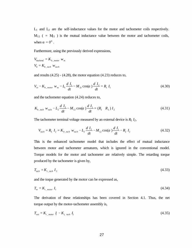
27

L1 and L2 are the self-inductance values for the motor and tachometer coils respectively.

M12 ( = M21 ) is the mutual inductance value between the motor and tachometer coils,

when α = 0ο .

Furthermore, using the previously derived expressions,

_

_

backemf b motor m

b b tach tach

V K

V K

ω

ω

=

=

and results (4.25) - (4.28), the motor equation (4.23) reduces to,

1 2_ m 1 21 1 1

cos( ) in b motor

d I d IV K L M R I

dt dtω α− − − = (4.30)

and the tachometer equation (4.24) reduces to,

2 1_ tach 2 12 2 2

cos( ) ( ) b tach L

d I d IK L M R R I

dt dtω α− − = + (4.31)

The tachometer terminal voltage measured by an external device is RL I2,

2 12 _ 2 12 2 2

cos( ) tach L b tach tach

d I d IV R I K L M R I

dt dtω α∴ = = − − − (4.32)

This is the enhanced tachometer model that includes the effect of mutual inductance

between motor and tachometer armatures, which is ignored in the conventional model.

Torque models for the motor and tachometer are relatively simple. The retarding torque

produced by the tachometer is given by,

_ 2 tach t tachT K I= (4.33)

and the toque generated by the motor can be expressed as,

_ 1 m t motorT K I= (4.34)

The derivation of these relationships has been covered in Section 4.1. Thus, the net

torque output by the motor-tachometer assembly is,

_ 1 _ 2 out t motor t tachT K I K I= − (4.35)

28

Equations (4.30) through (4.35) are the final results of this derivation. The signs

associated with each term in these equations are very important, as they can significantly

effect the system dynamics. At this stage we can consider making some simplifications.

A pragmatic observation is that I2 (load current) is much smaller than I1 (motor current).

In fact, if RL, the input impedance of the voltage-measuring device (e.g. SigLab) is high,

which it is in this case (~ 1 Μohm), then the current drawn from the tachometer is almost

negligible. We can therefore eliminate terms containing I2, wherever it occurs in

equations (4.30) - (4.35), which leads to some simplification. At this point however, we

shall retain the term ‘-R2 I2’ in the Vtach expression from equation (4.32). This is done to

resolve a singularity at a later stage. Since this term constitutes a damping term, the sign

associated with it is very important in determining the phase change at zero and pole

frequencies. In the absence of this term, the model sees a singularity and arbitrarily

assigns either a +180o or –180o phase change. A damping term, however small (even

negligible), resolves this singularity and determines whether this phase change has to be

+180o or –180o, depending upon the sign associated with this damping term. Thus, this

term is retained only to predict the phase plot in frequency response. It has no effect on

the magnitude plot whatsoever.

A final observation is made regarding the ‘-R2 I2’ term. Had the transformer effect been

an ideal one, the relationship (4.18) would hold, i.e., I2 = (N1/N2) I1. In the present case,

this is not true, since the transformer effect is a weak one. Nevertheless, I2 may be weakly

related to I1 by some empirical constant. Based on this argument, we suggest that ‘R2 I2’

may be replaced by ‘Kr I1’ where Kr is an experimentally determined empirical constant.

The validity of this empirical conjecture, though questionable at this stage, shall be

confirmed experimental measurements. Experimental verification is covered in the

following section.

Implementing these discussions, the motor-tachometer equations reduce to,

29

1_ m 1 1 1

1_ 12 2 2

_ 1

Motor Equation:

Tachometer Equation: cos( )

Torque Equation:

in b motor

tach b tach tach

out t motor

d IV K L R I

dtd I

V K M R Idt

T K I

ω

ω α

− − =

= − −

=

(4.36)

Comparing these results with the previous results, we notice that the motor model and the

torque expression remain the same, while the tachometer model has additional terms in it,

that were missing in the conventional model.

Rewriting the tachometer equation,

1_ 1

12

2 2 1

cos( ) (magnetic coupling constant)

( / ) (loading effect constant)

tach b tach tach m r

m

r

d IV K K K I

dtK M

K R I I

ω

α

= + −

−@@

(4.37)

This is final form of the enhanced tachometer model. Note that since the tachometer is

magnetically coupled to the motor, the motor current influences the tachometer terminal

voltage despite the fact that the two are electrically insulated. This model reduces to the

conventional model, given by equation (4.16), if the magnetic coupling constant Km = 0,

and the loading effect constant Kr = 0. These two constants are easily determined

experimentally, as shall be described in the next section. Kr is always positive, while Km

may be positive or negative depending on the angle α.

30

5. EXPERIMENTAL VERIFICATION OF THE PROPOSED MODEL


Variable Symbol

Motor angular position θm

Tachometer angular position θ t

Motor current im

Motor torque Tm

Tachometer voltage Vtach

Parameter Symbol Value Source

Motor armature inertia Jm 43.77e-6 kg-m2 Manf. Specs.

Tachometer armature inertia Jt 11.35e-6 kg-m2 Manf. Specs.

Motor-Tachometer shaft stiffness K 1763.2 N-m/rad Parameter ID

Motor torque constant Kt 8.33e-2 N-m/A Manf. Specs.

Tachometer constant Ktach 0.1377 V/rad/s Manf. Specs.

Magnetic Coupling constant Km 8.8852e-5 Henry Parameter ID

Loading effect constant Kr 2.6656e-2 Ohms Parameter ID

We now incorporate the tachometer model obtained in Section 4.3, in the analysis for the

motor-tachometer system that we studied earlier in Section 3. The transfer function of

mechanical system from equation (3.1) remains unchanged,

2 2 [ ( )]

t

m t m t m

KT s J J s K J Jθ

=+ +

(5.1)

DC motor operating in current mode can also be modeled as earlier,

m t m

m amp in

m amp t in

T K ii K V

T K K V

==

=

(5.2)

31

Based on Section 4.3, the tachometer output is now expressed as,

( / )tach tach t m m r mV K K di dt K iθ= + −& (5.3)

The expressions (5.1)–(5.3) yield the following overall transfer function for the unloaded

motor-tachometer system,

2

2

[ ( ) ( ) ]( )

( ) [ ( )]

t tachamp m rtach

in

t m t m

K K den s K den s K K KVV den s

den J J s K J J

− +=

+ +@ (5.4)

This analytically obtained transfer function for the tachometer-motor system is used to

generate the frequency response plots in MATLAB. These plots are then compared to the

experimentally obtained plots

Figure 5.1 Vtach/Vin : Comparison of analytically predicted and experimentally obtained frequency response plots for the motor-tachometer system

102

103

-40

-30

-20

-10

0

10

Mag

nitu

de d

B

Experimental: Solid Line Theoretically Predicted: Broken Line

102

103

-400

-300

-200

-100

0

Frequency (Hz)

Pha

se (d

egre

es)


Experimentally Obtained

Experimentally obtained


32

Some interesting observations made from the above comparison are listed here:

1. The new model predicts the experimental observation even for the high frequency

range very accurately. The analytical plot does indicate the presence of two complex-

conjugate zeros that are observed in the experimental plots.

2. Looking at the system transfer function given by equation (5.4), we can now explain

the presence of the additional zeros. It is evident that a positive Km leads to complex

conjugate zero pairs in the system. Clearly, these zeros will disappear for Km=0. In

this particular case we have two complex conjugate zero pairs which is one more than

the number of complex conjugate pole pairs.

3. The presence of Kr with a negative sign explains why the phase drops by 180o at the

first zero frequency. The loading effect pushes the first complex-conjugate pole pair

to the right side of the imaginary axis on the s-plane. The importance of the negative

sign associated with Kr becomes evident here, which is why signs were dealt with

care during the derivation of the tachometer model.

4. Although the conventional model predicted the system poles accurately, it failed to

explain the presence of system zeros. The new model addresses this inconsistency

very well.

Once the new tachometer model is experimentally confirmed, the results of the above

experimental plots are then used to back-calculate the exact values of the parameters K

(shaft stiffness), Km (magnetic coupling constant) and Kr (loading effect constant). In

Figure 5.1, the first zero frequency is 247 Hz, and the second zero frequency is 2200 Hz.

The pole next to the second zero is at 2230 Hz. Equating the predicted pole frequency

expression to experimentally obtained frequency, we get K=1763.2 N-m/rad. Equating

the predicted zero frequency expressions to experimentally obtained zero frequencies, we

get Km=8.62565e-5 Henry. From the experimental plot, the damping at the first pole is

estimated to be ζ= 0.098. Equating this to the theoretically predicted expression for

damping, we get Kr=2.6656e-2 Ohms. Note that Km and Kr are very small numbers.

33

5.1 Discussion on the proposed tachometer model

We thus see that for an accurate prediction of experimental results, the simple ‘gain’

model for tachometer is not sufficient. An accurate tachometer model is developed in the

preceding sections. We now state some observations/conclusions based on the new

model:

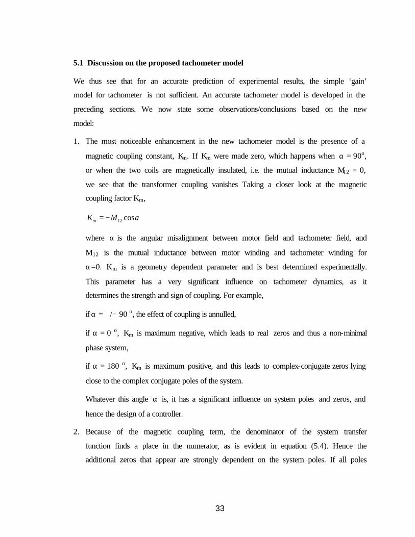
1. The most noticeable enhancement in the new tachometer model is the presence of a

magnetic coupling constant, Km. If Km were made zero, which happens when α = 90o,

or when the two coils are magnetically insulated, i.e. the mutual inductance M12 = 0,

we see that the transformer coupling vanishes Taking a closer look at the magnetic

coupling factor Km,

12 cosmK M α= −

where α is the angular misalignment between motor field and tachometer field, and

M12 is the mutual inductance between motor winding and tachometer winding for

α=0. Km is a geometry dependent parameter and is best determined experimentally.

This parameter has a very significant influence on tachometer dynamics, as it

determines the strength and sign of coupling. For example,

if α = +/− 90 o, the effect of coupling is annulled,

if α = 0 o, Km is maximum negative, which leads to real zeros and thus a non-minimal

phase system,

if α = 180 o, Km is maximum positive, and this leads to complex-conjugate zeros lying

close to the complex conjugate poles of the system.

Whatever this angle α is, it has a significant influence on system poles and zeros, and

hence the design of a controller.

2. Because of the magnetic coupling term, the denominator of the system transfer

function finds a place in the numerator, as is evident in equation (5.4). Hence the

additional zeros that appear are strongly dependent on the system poles. If all poles

34

are complex-conjugate pairs, and if Km is positive, then all the resulting zeros are also

complex conjugate pairs, and the number of these zero pairs is one greater than the

number of complex conjugate pole pairs (excluding the poles at the origin).

3. The other important parameter that appears in proposed tachometer expression is the

empirical constant Kr, which is always positive. Once again, since Kr is dependent on

the experimental set-up, it is best obtained experimentally. If the additional zeros are

complex conjugate, the negative sign associated with Kr pushes them slightly into the

right half of s-plane. This phenomenon helps in predicting the phase change at the

zero frequencies in the phase vs. frequency plots.

4. The significance of the signs associated with Kr and Km is now evident since these

signs dictate the nature and location of the additional zeros. This is the reason why the

importance of signs was emphasized during the derivation of the tachometer model.

35

6. TYPICAL APPLICATION: MOTION CONTROL IN PRESENCE OF SHAFT

COMPLIANCE


Variable Symbol

Motor angular position θm

Tachometer angular position θ t

Inertia 1 angular position θ1

Inertia 2 angular position θ2

Motor current im

Motor torque Tm

Tachometer voltage Vtach

Parameter Symbol Value

Motor armature inertia Jm 43.77e-6 kg-m2

Tachometer armature inertia Jt 11.35e-6 kg-m2

Inertia 1 J1 18.77e-6 kg-m2

Inertia 2 J2 18.77e-6 kg-m2

Motor-Tachometer shaft stiffness K 1763 N-m/rad

Torsional stiffness of Shaft 1 Kshaft1 623 N-m/rad

Torsional stiffness of Shaft 2 Kshaft2 1063 N-m/rad

Torsional stiffness of coupling Kcoupling 1500N-m/rad

Effective torsional stiffness of Shaft 1, Shaft2 and coupling (in series)

K1 311 N-m/rad

Torsional stiffness of Shaft 3 K2 249 N-m/rad

Motor torque constant Kt 8.33e-2 N-m/A

Tachometer constant Ktach 0.1377 V/rad/s

Magnetic Coupling constant Km 8.8852e-5 Henry

Loading effect constant Kr 2.6656e-2 Ohms

Voltage to current amplification Kamp 0.5 A/V

36

We now consider a typical problem in DC motor motion control using tachometer

feedback. The integrated motor-tachometer assembly described in Section 2 is used. The

motor shaft is now connected to a load by means of a flexible coupling of known

stiffness. Furthermore the load is in the form of two inertia’s connected by a shaft. Thus

the system has multiple flexible elements.

Figure 6.1 Motor-tachometer-load System

A lumped parameter model is used to describe the above system, with the assumption

that dissipation terms (i.e. Coulomb friction, viscous damping and material damping)

hardly influence the existence of system poles and zeros. As was discussed in Section 3,

the purpose of the present investigation is to identify the poles and zeros of the overall

system that arise due to the mechanical and electromagnetic characteristics of the system.

From a frequency response perspective, mechanical damping does not govern the

existence of these poles and zeros. It only tends to reduce their intensity as was illustrated

in Figure 3.2. A more rigorous distributed parameter model with all dissipation terms

included can be used to get a much more exact match between the zero and pole locations

in the experimental and predicted plots. We do not use such a model here because the

simple lumped parameter model with no dissipation assumption is sufficient to capture all

the prominent attributes that are noticed in the experimental results. Our objective here is

Motor

Tach FlexibleCoupling Inertia1 Inertia2

Shaft1 Shaft2

Shaft3

37

to show the significant extent by which the new model changes the analytical predictions

and indeed brings them very close to the experimental observations.

A physical model of the above system is shown below,

Figure 6.2 Physical Model of the motor-tachometer-load system

Drawing free-body diagrams for each of the four inertias and applying Newton’s II Law,

we arrive at the following transfer function for mechanical system,

2

[ ][ ]

t

m

numT s denθ

=⋅

(6.1)

where,

4 2 1 2 1 2 2 1 2 2 1 2

6 1 2

4 2 1 1 2 2 2

1 2 1 2 1 1 2

2 1 2

[ ] [ ( ) ]

[ ] [ ]

[ ]

[

t m

t m t m t m

m t t

t

num K J J s J K J K J K s K K

den s J J J J

s K J J J K J J J K J J JK J J J K J J J K K J J

s K K J

= + + + +

= +

+ + ++ + +

2 1 1 2

2 2 2 1 1 2

2 2 1 2 1 1 1 2 1 2 1 2

1 2 1 2

] [ ( )]

m m m

m t t

t t

t m

J K K J J K K J JK K J J K K J J K K J J

K K J J K K J J K K J J K K J JK K K J J J J

+ ++ +

+ + ++ + + +

(6.2)

The motor model is same as earlier,

Jt JmJ1 J2

θt θ1 θ2

θm

Tm

38

m t m

m amp in

m amp t in

T K ii K V

T K K V

==

=

(6.3)

The new tachometer model is given by equation (4.37),

( / )tach tach t m m r mV K K di dt K iθ= + −& (6.4)

All these expressions (6.1)-(6.4) lead to the following overall system transfer function,

2 [ ( ) ( ) ( )]

( )amp m r t tachtach

in

K K s den K s den K K numVV s den

− += (6.5)

On the other hand, if we were to obtain the system transfer function using the

conventional tachometer model, given by equation (4.16), we get the following

( )

( )amp t tachtach

in

K K K numVV s den

= (6.6)

Comparing the two transfer functions (6.5) and (6.6), it is clear that the new model

captures some dynamics that is missing in the old model. Note that, in (6.5) if Kr = Km =

0, then (6.5) reduces to (6.6).

Next we perform a sine-sweep experiment on the actual system to obtain its frequency

response experimentally. We compare the experimentally obtained frequency plots with

those predicted by the two models. Figure 6.3 presents a comparison of the experimental

frequency plots with those predicted by the old model, expression (6.6). Figure 6.4

presents a comparison of the experimental results with the predictions of the new model,

expression (6.5)

39

Figure 6.3 Vtach/Vin : Comparison of experimental frequency response and predicted frequency response using conventional model

Figure 6.4 Vtach/Vin : Comparison of experimental frequency response and predicted frequency response using proposed model

101

102

103

-50

-40

-30

-20

-10

0

10

Mag

nitu

de (d

B)

Experimental: Solid Line Theortically predicted: Broken Line

101

102

103

-800

-600

-400

-200

0

Freq (Hz)

Pha

se (d

eg)

40

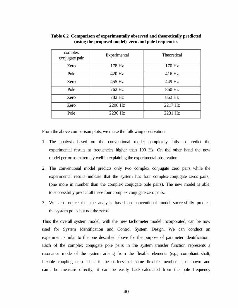
Table 6.2 Comparison of experimentally observed and theoretically predicted (using the proposed model) zero and pole frequencies

complex

conjugate pair Experimental Theoretical

Zero 178 Hz 170 Hz

Pole 420 Hz 416 Hz

Zero 455 Hz 449 Hz

Pole 762 Hz 860 Hz

Zero 782 Hz 862 Hz

Zero 2200 Hz 2217 Hz

Pole 2230 Hz 2231 Hz

From the above comparison plots, we make the following observations

1. The analysis based on the conventional model completely fails to predict the

experimental results at frequencies higher than 100 Hz. On the other hand the new

model performs extremely well in explaining the experimental observation

2. The conventional model predicts only two complex conjugate zero pairs while the

experimental results indicate that the system has four complex-conjugate zeros pairs,

(one more in number than the complex conjugate pole pairs). The new model is able

to successfully predict all these four complex conjugate zero pairs.

3. We also notice that the analysis based on conventional model successfully predicts

the system poles but not the zeros.

Thus the overall system model, with the new tachometer model incorporated, can be now

used for System Identification and Control System Design. We can conduct an

experiment similar to the one described above for the purpose of parameter identification.

Each of the complex conjugate pole pairs in the system transfer function represents a

resonance mode of the system arising from the flexible elements (e.g., compliant shaft,

flexible coupling etc.). Thus if the stiffness of some flexible member is unknown and

can’t be measure directly, it can be easily back-calculated from the pole frequency

41

locations obtained from experimental data and an accurate knowledge of the complete

system model. This was done in Section.5, where the motor-tachometer shaft stiffness

was estimated from the frequency response plots. Apart from parameter identification,

the new tachometer model has significant implications in terms of controller design for

achieving close-loop stability. These issues are discussed in the following section.

42

7. CONTROL SYSTEM DESIGN

7.1 Introduction

The objective of this exercise in control system design is to achieve a closed loop stable

servo system for positioning the load inertia accurately using tachometer feedback, with

reference to the system described in Section 6 (Figure 6.1). We know that compliance in

a system, if not accounted for adequately in the controller design, leads to closed loop

instability [4, 6, 9, 10], which in this case manifests itself as a high-pitch ringing.

We want to make sure that the compensator addresses all the high frequency open-loop

poles and zeros resulting from flexible elements and that the compensated close-loop

system has no poles on the right side of s-plane. It is observed that, if there is a high

frequency pole in the open-loop system, its effect can never be completely eliminated.

Since close-loop poles lie on the root-loci emanating from open-loop poles, there will a

corresponding high frequency poles in the close-loop system as well. This is further

clarified in the following sections. Nevertheless, by means of appropriate compensator

design, we usually can ensure that the effect of these closed-loop poles on system

stability is not detrimental. For close-loop stability, the closed-loop poles should all lie on

the left side of the s-plane. If, for any reason, the closed-loop poles get too close to the

imaginary axis or, even worse, spill over into the right side of the s-plane, then we can

expect the undesirable phenomenon of high-frequency ringing in the closed-loop

operation of the system. Since the objective is to eliminate this high frequency ringing

during high-speed and high-precision closed loop operation, we shall proceed with the

above discussion in mind.

The following three issues make the control design for the system in consideration

interesting as well as complex:

1) This is a case of multiple inertias connected by flexible elements, with the sensor and

actuator being noncolocated. While the torque is applied to the motor rotor, the

angular measurement is made at the tachometer rotor. This necessitates the study of

colocated and non-colocated systems.

43

2) The tachometer does not precisely measure the tachometer-rotor angular velocity. The

tachometer has sensor dynamics, which adulterates the velocity signal and reshuffles

the system zeros (as discussed earlier in Section 5). In fact the tachometer dynamics

makes the system a non-minimum phase system, since some zeros introduced by the

tachometer lie on the right hand side of the s plane.

3) Although while measuring the tachometer rotor angle, we are trying to position the

load inertia. Normally, it is possible to control only those system states that can be

measured or estimated. In this case we are trying to control the load position, which is

not actually being measured. In this context, it is important to note that, since the

system is relatively very stiff, positioning the motor/tachometer rotor will lead to a

positioning of load inertia. It tachometer angle is used for feedback control, then the

tachometer rotor will attain the commanded position very quickly, while the load

inertia may have a slightly higher settling time. If ensuring closed-loop stability is the

primary objective (i.e. eliminate high-pitch ringing) then this is not a problem. As

long as any one transfer function (say tachometer angle vs. motor input torque) is

used for designing a stable closed loop, the entire system is stabilized. All poles of all

the close-loop transfer functions will have poles restricted to the left side of the s-

plane. Despite this, if very fast and accurate positioning of the load inertia were the

main concern, then it is a better choice to measurements at the load end rather than

the motor end. Once again if we design a suitable controller to make the load-angle

vs. motor-torque transfer function stable in close-loop, the entire system becomes

stable i.e., there are no unstable poles in any transfer function of the system, and

hence no high frequency ringing. But now motor and tachometer inertias shall have a

longer settling time.

Before we deal with the actual system, let us investigate the above three issues one by

one for ease of comprehension. Once we understand each one of these individually, we

shall be able to study the combined effect of all these on the system in consideration.

44

7.2 Colocated and Noncolocated Control

7.2.1 Two-mass single-spring system

Although there will be damping (material, viscous or Coulomb) present in any real

system, for the following discussion the damping terms have been neglected. Since the

present objective is to study the occurance and significance of poles and zeros in a

system, this assumption is acceptable.

Throughout the following discussion, the term ‘pole’ should be interpreted as a complex-

conjugate pole pair and ‘zero’ should be interpreted as a complex-conjugate zero pair.

For simplicity, initially the following two-mass single-spring system is considered. Free

body diagrams for each mass are drawn.

m1 m2

Fin

x1 x2

k

m1 m2

Fin

k(x1-x2) k(x1-x2)

Figure 7.1 Two-mass single-spring system

Application of Newton’s II Law leads to,

2 1 1 1

1 2 2 2

( )( )inF k x x m x

k x x m x+ − =

− =

&&&& (7.1)

45

After a few algebraic manipulations, we obtain the following transfer functions

21 2

2 21 2 1 2

22 2

1 2 1 2

[ ( )]

[ ( )]

in

in

x m s kF s m m s k m m

x kF s m m s k m m

+=

+ +

=+ +

(7.2)

22

1 2

x kx m s k

=+

(7.3)

Thus, the pole frequency is 2

2 1

1k mm m

+

, and the zero frequency is

2

km

(7.4)

Frequency (rad/sec)

Pha

se (

deg)

; Mag

nitu

de (

dB)

Bode Diagrams

-80

-60

-40

-20

0

20From: U(1)

100 101-400

-350

-300

-250

-200

-150

To: Y

(1)

Fig 7.2 Bode plot for x1 / Fin transfer function

46

Frequency (rad/sec)

Pha

se (

deg)

; Mag

nitu

de (

dB)

Bode Diagrams

-60

-40

-20

0

20

40From: U(1)

100 101-400

-350

-300

-250

-200

-150

To:

Y(1

)

Fig 7.3 Bode plot for x2 / Fin transfer function

In this two-mass single-spring case, the 1

in

xF transfer function is referred to as a

colocated transfer function, since the actuator and sensor are mounted on the same mass.

Whereas the 2

in

xF transfer function is referred to as the noncolocated transfer function

since the sensor and the actuator are mounted on different masses. It is important to note

that for the colocated case, each pole is preceded by a zero, and hence there are

alternating poles and zeros along the imaginary axis in the root-locus diagram. Quite

unlike this, for the noncolocated case, every pole is not preceded by a zero. Since, poles

are characteristic of the system, each transfer function in the system (colocated as well as

non-colocated) exhibits the same poles. On the other hand, zeros depend upon the sensor

and actuator location. If the two are colocated then, as mentioned earlier, there are as

47

many zeros as the number of poles. If the two are not colocated then the number of zeros

falls short of the number of poles of the system.

7.2.2 Open-loop characteristics: Physical significance of poles and zeros

Let us try to understand the physical significance of poles and zeros and subsequently

relate this understanding to the mathematically obtained conclusions. Based on the

discussions in Section 7.2.1, we make the following observations

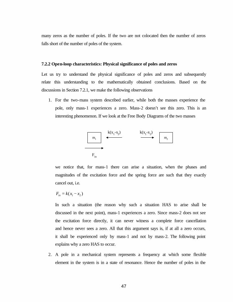
1. For the two-mass system described earlier, while both the masses experience the

pole, only mass-1 experiences a zero. Mass-2 doesn’t see this zero. This is an

interesting phenomenon. If we look at the Free Body Diagrams of the two masses

m1 m2

Fin

k(x1-x2) k(x1-x2)

we notice that, for mass-1 there can arise a situation, when the phases and

magnitudes of the excitation force and the spring force are such that they exactly

cancel out, i.e.

1 2( )inF k x x= −

In such a situation (the reason why such a situation HAS to arise shall be

discussed in the next point), mass-1 experiences a zero. Since mass-2 does not see

the excitation force directly, it can never witness a complete force cancellation

and hence never sees a zero. All that this argument says is, if at all a zero occurs,

it shall be experienced only by mass-1 and not by mass-2. The following point

explains why a zero HAS to occur.

2. A pole in a mechanical system represents a frequency at which some flexible

element in the system is in a state of resonance. Hence the number of poles in the

48

system transfer function is equal to the number resonance modes of the system.

Poles are characteristics of the system and are therefore experienced by all the

masses. Once again referring to the two-mass single-spring system which has only

one pole corresponding to a resonance in the spring. Let us first try to understand

what this resonance physically means. At the resonance frequency, an

infinitesimally small excitation force produces a large sustained motion in the

system. Ideally, if there is no energy loss, then the system should exhibit violent

oscillations even for zero excitation force. If the excitation force, which is also the

net external force on the system, is zero, then total momentum of the system has

to be conserved, i.e.,

1 1 2 2 1 1 2 20 m x m x m x m x+ = ⇒ = −& & & &

during resonance. This shows that at the resonance frequency, the two masses

move 180o out of phase.

m1 m2

k

Now let us take a look at what happens at lower frequencies, and visualize the

state of the system while gradually increasing the frequency.

Stage I: Rigid Body; excitation frequency close to 0

m1 m2

At low frequencies the two bodies move in phase with each other as though they

were rigidly fixed. This is called the rigid body mode ( 1 2x x=& & ). Referring to

equations Error! Reference source not found., we conclude the following

49

1 2

1 2( )in

x x xF m m x

= == +

&& && &&&& (7.5)

Stage II: Resonance; excitation frequency close to pole frequency

Between the initial stage (Stage I) when the two masses move in phase, and the

resonance stage (Stage II) when the masses move out of phase, there has to be an

intermediate stage where a transition from synchronism to asynchronism occurs.

One of the two masses that are moving in phase has to come to a complete stop

and then start moving in the opposite phase. This stage corresponds to a zero

occurs at the zero frequency. As explained in the previous section, if there is a

zero stage, the zero shall be experienced by mass-1 and not mass-2.

m1 m2

Very Low Frequency

m1 m2

Zero Frequency

m1 m2

Pole Frequency

Figure 7.4 System frequency response when excitation force is applied on

mass-1

50

This observation is verified by the transfer function between x2 and x1,

22

1 2

x kx m s k

=+

and it becomes very clear from the Bode Plot presented in the following figure

Frequency (rad/sec)

Pha

se (

deg)

; Mag

nitu

de (

dB)

Bode Diagrams

-50

0

50

100From: U(1)

100 1010

50

100

150

200

To:

Y(1

)

Figure 7.5 Bode plot for x2 / x1 transfer function

Thus, zero frequency is the frequency at which the masses lose synchronism and fall out

of phase. This leads to a very significant conclusion: For a purely mechanical system, a

resonance frequency is always preceded by a zero frequency. For a resonance to occur,

the two masses have to be out of phase, and this happens only at the zero frequency.

Hence, since the zero sets the stage for the resonance, it has to occur before the pole. In

other words, the zero frequency is always less than the pole frequency. What we have

concluded by physical reasoning is exactly the same as what was predicted by

51

mathematical derivation in expressions (7.2)-(7.4). A similar discussion on poles and

zeros is provided by Welch [4].

7.2.3 Closed-loop characteristics: Stability Analysis

In the previous sub-section, we discussed the open-loop characteristics of the two-mass

single-spring system. In this section we shall try to concentrate on the closed-loop

characteristics of the same system. We shall investigate the stability of the closed loop

system by looking at the root-locus and frequency plots of the open loop system. Once

again, let us rewrite the two relevant transfer functions for the system

221 1

1 22 21

2 222 2

1

1 1

2

Colocated Case( )

Noncolocated Case( )

(shown earlier)1

in

in

in

x s zk

F s s px kF s s pz px

F s

+=

+

=+

<

= Rigid Body Case

where z1 is the zero and p1 is the pole, as given by expressions (7.2)-(7.4).

Each of these cases is studied individually and the compensator designs that make the

respective systems stable in close-loop are presented. We also consider the case of a rigid

body that has no flexible elements and compare it with the above two cases in terms of

closed loop stability.

Rigid Body Case: 2

1

in

xF s

=

Without any compensator the root-locus and frequency plots for the system are as

follows,

52

-1 -0.8 -0.6 -0.4 -0.2 0 0.2 0.4 0.6 0.8 1-1.5

-1

-0.5

0

0.5

1

1.5

Real Axis

Imag

Axi

s

Fig. 7.6(a) Root-locus for the rigid body case ( 21

s)

Frequency (rad/sec)

Pha

se (

deg)

; Mag

nitu

de (

dB)

Bode Diagrams

-100

-50

0

50From: U(1)

10-1 100 101 102-181

-180.5

-180

-179.5

-179

To:

Y(1

)

Fig. 7.6(b) Bode plots for the rigid body case ( 21

s)

53

From the root locus it is clear that the system is marginally stable for any value of gain,

since the close-loop poles always lie on the imaginary axis. This is confirmed from the

Bode plots, which indicate that for any gain, the Phase Margin is always zero. Hence the

system is at the margin of stability. If we add a lead compensation to the plant, then the

above two plots get modified as follows:

-6 -5 -4 -3 -2 -1 0 1 2-4

-3

-2

-1

0

1

2

3

4

Real Axis

Imag

Axi

s

Fig. 7.7(a) Root-locus for the rigid body case with lead compensation ( 2

2ss+

)

54

Frequency (rad/sec)

Pha

se (

deg)

; Mag

nitu

de (

dB)

-50

0

50

100Gm=-319.09 dB (at 0 rad/sec), Pm=38.668 deg. (at 1.6005 rad/sec)

10 -2 10-1 100 101-180

-160

-140

-120

-100

Fig. 7.7(b) Bode plot for the rigid body case with lead compensation ( 2

2ss+

)

From these new plots it is clear that the lead compensator (real zero in the numerator)

stabilizes the closed loop system by adding phase to the open-loop system. In the root-

locus plots, the compensator zero has pulled the root-loci branches to the left side of the

s-plane, thus making the closed loop system stable for any gain. On the other hand

looking at the Bode plot we see that the system has infinite Gain Margin, since the phase

asymptotically approaches –180o. Also for any gain and therefore for any cross-over

frequency, there is a positive Phase Margin. When the gain is very low, the cross-over

frequency is also low which leads to a very small Phase Margin. This corresponds to the

fact that now the closed-loop poles on the root-locus plot are very close to the imaginary

axis. For high gains, the Bode plots predict a maximum phase margin of 90o. On the root-

locus this corresponds to the fact that now the close-loop poles lie on the negative real

axis, thus making the system very stable. In any case, we notice that it is very easy to

stabilize the rigid body mode transfer function. Thus if there are no flexible elements in a

55

system, then close-loop instabilities are easily avoided. Now let us see how the presence

of a spring in the system changes this situation.

Colocated Case: 22

1 122 2

1( )in

x s zF s s p

+=

+

For the colocated case we observe that other than the two poles at the origin, the system

also has a pole-zero pair. As was observed earlier, the zero frequency is always less than

the pole frequency. In the case of multiple flexible elements, an important feature of the

colocated transfer function is the pole-zero alternation as one moves along the imaginary

axis. This property will be of immense use in the design of a compensator as shall be seen

shortly.

-0.5 -0.4 -0.3 -0.2 -0.1 0 0.1 0.2 0.3 0.4 0.5-6

-4

-2

0

2

4

6

Real Axis

Imag

Axi

s

Fig. 7.8(a) Root-locus plot for the uncompensated colocated system (22

122 2

1( )s z

s s p++

)

56

Frequency (rad/sec)

Pha

se (

deg)

; Mag

nitu

de (

dB)

Bode Diagrams

-40

-30

-20

-10

0From: U(1)

100 101-200

-150

-100

-50

0

To: Y

(1)

Fig 7.8(b) Bode plots for the uncompensated colocated system (22

122 2

1( )s z

s s p++

)

Note that a small amount of damping has been added (although not indicated in the

transfer function) while obtaining these plots to make them more realistic. From the root-

locus of the uncompensated colocated system, it is evident that the system will only be

marginally stable for any value of gain. Similarly, the Bode plots show that for any open-

loop gain the Phase Margin will be very small, nevertheless positive. Next, we study the

effect of a lead compensator on this system.

57

-6 -5 -4 -3 -2 -1 0 1 2-4

-3

-2

-1

0

1

2

3

4

Real Axis

Imag

Axi

s

Fig 7.9(a) Root-locus plot for the compensated colocated system: 22

122 2

1

( 2)( )s z

ss s p

++

+

Here the root-locus indicates that the system will be unconditionally stable for all gains.

For very low and very high gains, the closed-loop poles are quite close to the imaginary

axis. These observations are confirmed from the Bode plots as well. For any value of gain

the system has a positive gain margin. For a low open-loop gain, resulting in a low

crossover frequency, the phase margin (although positive) is very close to zero. Once

again, for the colocated case we see that it is fairly easy to stabilize the closed loop

system by means of a simple lead controller. It is important to mention here that this has

been possible only due to the fact that the zero occurs before the pole, which adds phase

to the system at the right frequency. Had this not been the case, close-loop instability

would have existed.

58

Frequency (rad/sec)

Pha

se (

deg)

; Mag

nitu

de (

dB)

Bode Diagrams

-40

-20

0

20

40

60

10-1

100

101

-200

-150

-100

-50

0

50

Fig. 7.9(b) Root-locus plot for the compensated colocated system: 22

122 2

1

( 2)( )s z

ss s p

++

+

Noncolocated Case: 222 2

1

1( )in

xF s s p

=+

In the noncolocated case, a distinct feature is that not all poles have a zero that precedes

them. In fact for the two-mass single-spring case, the noncolocated transfer function has

no zeros at all. The root-locus and bode plots for this case are presented in the following

figures. Clearly, from the root-locus the uncompensated system is unstable for any gain,

high or small. At the same time, Bode plots indicate that for any open-loop gain, the

Phase margin will be negative. For extremely small gains, the phase margin approaches

zero but from the negative side. Hence the system is always unstable.

59

-1 -0.8 -0.6 -0.4 -0.2 0 0.2 0.4 0.6 0.8 1-4

-3

-2

-1

0

1

2

3

4

Real Axis

Imag

Axi

s

Fig. 7.10(a) Root-locus for the uncompensated noncolocated system ( 22 21

1( )s s p+

)

Frequency (rad/sec)

Pha

se (

deg)

; Mag

nitu

de (

dB)

Bode Diagrams

-80

-60

-40

-20

0

100 101-400

-350

-300

-250

-200

-150

Fig. 7.10(b) Bode plots for the uncompensated noncolocated system ( 22 21

1( )s s p+

)

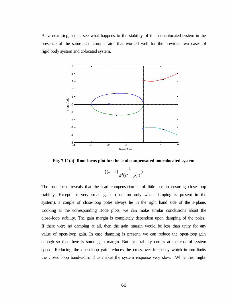
60

As a next step, let us see what happens to the stability of this noncolocated system in the

presence of the same lead compensator that worked well for the previous two cases of

rigid body system and colocated system.

-4 -3 -2 -1 0 1 2-5

-4

-3

-2

-1

0

1

2

3

4

5

Real Axis

Imag

Axi

s

Fig. 7.11(a) Root-locus plot for the lead compensated noncolocated system

( 22 21

1( 2)

( )s

s s p+

+)

The root-locus reveals that the lead compensation is of little use in ensuring close-loop

stability. Except for very small gains (that too only when damping is present in the

system), a couple of close-loop poles always lie in the right hand side of the s-plane.

Looking at the corresponding Bode plots, we can make similar conclusions about the

close-loop stability. The gain margin is completely dependent upon damping of the poles.

If there were no damping at all, then the gain margin would be less than unity for any

value of open-loop gain. In case damping is present, we can reduce the open-loop gain

enough so that there is some gain margin. But this stability comes at the cost of system

speed. Reducing the open-loop gain reduces the cross-over frequency which in turn limits

the closed loop bandwidth. Thus makes the system response very slow. While this might

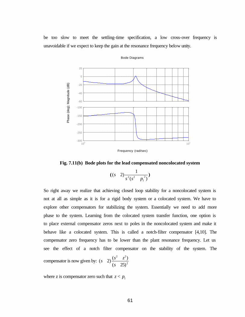
61

be too slow to meet the settling-time specification, a low cross-over frequency is

unavoidable if we expect to keep the gain at the resonance frequency below unity.

Frequency (rad/sec)

Pha

se (

deg)

; Mag

nitu

de (

dB)

Bode Diagrams

-60

-40

-20

0

20

100 101-300

-250

-200

-150

-100

Fig. 7.11(b) Bode plots for the lead compensated noncolocated system

( 22 21

1( 2)

( )s

s s p+

+)

So right away we realize that achieving closed loop stability for a noncolocated system is

not at all as simple as it is for a rigid body system or a colocated system. We have to

explore other compensators for stabilizing the system. Essentially we need to add more

phase to the system. Learning from the colocated system transfer function, one option is

to place external compensator zeros next to poles in the noncolocated system and make it

behave like a colocated system. This is called a notch-filter compensator [4,10]. The

compensator zero frequency has to be lower than the plant resonance frequency. Let us

see the effect of a notch filter compensator on the stability of the system. The

compensator is now given by: 2 2

2

( )( 2)

( 25)s z

ss

++

+

where z is compensator zero such that 1z p<

62

The overall open-loop transfer function for the compensated system now becomes

2 2

22 2 21

( ) 1( 2)

( 25) ( )s z

ss s s p

++

+ +

-12 -10 -8 -6 -4 -2 0 2-8

-6

-4

-2

0

2

4

6

8

Real Axis

Imag

Axi

s

Fig. 7.12(a) Root-locus plot for the notch compensated noncolocated system

63

Frequency (rad/sec)

Pha

se (

deg)

; Mag

nitu

de (

dB)

Bode Diagrams

-150

-100

-50

0

10-1 100 101 102-300

-200

-100

0

100

Fig. 7.12(b) Bode plots for the notch compensated noncolocated system

The two real poles in the compensator are necessary because the compensator zeros add

gain to the system at high frequencies thus making it susceptible to noise. The two poles

are placed far enough on the real axis so that their effect on stability is minimal, but at the

same time they ensure noise rejection at high frequencies. The zeros essentially add a 180

degrees phase at frequencies close to the system resonance frequency thus making it

close-loop stable. The problem with the resonance pole is that it leads to a phase lag of

180 degrees, which becomes detrimental for the close-loop stability.

From the above root-locus plots we conclude that the system is now stable except for

extremely high gains. The bode-plots indicate a positive phase margin for most values of

open-loop gain. For very high gains though, the phase margin becomes negative. The

notch-filter compensator for noncolocated systems is robust as long as the compensator

zero frequency is less than the plant resonance frequency. In case some parameter

variation causes the compensator zero to fall after the pole, a phenomenon called zero-

pole flipping, the system stability is jeopardized. Such an effect is extremely detrimental

64

for the system as is shown in the following figures. Pole-zero flipping may also occur

with the natural zeros in a non-colocated system. This issue is discussed in the following

sections.

-12 -10 -8 -6 -4 -2 0 2-8

-6

-4

-2

0

2

4

6

8

Real Axis

Imag

Axi

s

Fig. 7.13(a) Root-locus for the notch compensated noncolocated system in the

presence of pole-zero flipping

65

Frequency (rad/sec)

Pha

se (

deg)

; Mag

nitu

de (

dB)

Bode Diagrams

-150

-100

-50

0

10-1 100 101 102-300

-250

-200

-150

-100

Fig. 7.13(b) Bode plots for the notch compensated noncolocated system in the

presence of pole-zero flipping

As is clear from the above plots, the compensator zero does add phase to the system, but

at such a frequency that the phase margins are not improved at all. In fact, when a pole-

zero flipping occurs, the system becomes unconditionally unstable. In case the system has

some damping, the closed-loop system may be stable for very low or very high gains.

This is evident from the Bode plots which show that a positive phase margin exists for

very low and high gains.

In such a situation the compensator is no longer robust. Hence care should be taken while

implementing a notch-filter controller. In fact, for a robust compensator design, many

authors recommend the use of an optimal state-space controller [6,10]. A robust Linear

Quadratic Guassian (LQG) compensator design is presented by Cannon [10].

66

7.2.4 Multiple Mass Systems

We now extend the ideas developed in Sections 7.2.1-7.2.3 to multiple mass systems. For

a multiple-mass system with multiple flexible elements, like the one shown in Fig. 7.14

m1 m2

x1 x2

mn-1 mn

xn-1 xn

k1 kn-1

Fig. 7.14 Multiple-mass multiple-spring system

the system has as many resonance modes as the number of flexible elements (as long as

there are no closed chains in the system). Each of these resonance modes corresponds to a

complex-conjugate pole pair.

From another perspective, the system has as many modes of motion as the degrees of

freedom of the system. Thus if the system has four masses then there will be four

complex-conjugate pole pairs (including the pair at origin which corresponds to the rigid

body mode). Excluding the rigid body mode, the system therefore has three resonance

modes. These resonance modes are characteristics of the system and hence are

experienced by each mass in the system.

If an excitation force is applied on one of the masses in the above system, then we can

obtain transfer functions between the various system coordinates (x1,x2…xn) and the

input force. One of these will be a colocated case, wherein the actuator and sensor are

mounted on the same mass. All other transfer functions are the noncolocated cases.

Nevertheless, the poles of each of these transfer functions are the same, since poles are

characteristic of the entire system. As was discussed in Section 7.2.1, to set the stage for

each pole (i.e. resonance) a zero has to precede the resonance. Now this zero is

67

experienced only by some of the masses depending upon the actuator location, giving rise

to colocated and noncolocated cases.

For the colocated case, the mass on which the actuator force is applied experiences all the

zeros that precede the poles and hence the number of zeros in the colocated transfer

function is equal to the number of non-zero poles of the system. It is important to note

that for the colocated case, since each pole is preceded by a zero, there are alternating

poles and zeros along the imaginary axis in the root-locus diagram. As seen earlier, this

makes the control design problem very amenable. Even a simple lead compensator

provides a robust control action.

On the other for the non-colocated cases, the number of zeros experienced by any mass

falls short of the maximum possible number, by the number of coordinates (or masses)

that separate the sensor and the actuator. Also in this case parameter variation can lead to

the undesirable phenomena of pole-zero flipping. As an example consider the following

four-mass system.

m1 m2

x1 x2

m3 m4

x3 x4

k1 k3k2

Fin

Fig. 7.15 Four-mass three-spring system

The system has three resonance modes and hence 3 non-zero complex-conjugate pole

pairs. It also has one rigid body mode which results in a pole pair at the origin. While

mass-2 experiences three zeros since the actuator force acts on it, the other masses

experience fewer zeros. The x1/Fin and x2/Fin transfer functions have two zeros each,

while the x4/Fin transfer function has only one. The three resonance modes of the system

can occur in any order depending upon the mass and spring stiffness values. The single

zero in the x4/Fin transfer function corresponds to a zero before one of the three resonance

68

modes. Since the order of the resonance modes can vary depending upon the system

parameters, the single zero can occur before the first resonance, or between the first and

second resonance, or between the second and third resonance. This phenomenon is

known as pole-zero flipping and as was demonstrated earlier can jeopardize the close-

loop system stability since it drastically changes the root-locus and frequency response

plots. Therefore, during the compensator design for non-colocated systems it is necessary

to be aware of this problem and make sure that the compensator is robust enough to

handle this sudden change in phase and gain plots.

Let us see the close-loop behavior of this noncolocated transfer function in the presence

of a lead compensator (which of course is not sufficient to stabilize the system). In the

first case the zero lies between the first two resonance poles while in the second case it

lies between the last two poles.

Fig. 7.16(a) Pole-zero flipping in a noncolocated system

69

Fig. 7.16(b) Pole-zero flipping in a noncolocated system

70

7.3 Tachometer-Motor-Load System

Now that we have understood the fundamentals of colocated and noncolocated controls

with reference to multiple-mass multiple-spring systems, we are in a position to focus our

attention on the system in consideration, the tachometer-load-inertia system.

Fig. 7.17 Physical System and Physical Model

Since the actuator torque is applied at the motor rotor, and the speed is sensed at the

tachometer, the transfer function is noncolocated. Referring to Section 6 and equations

(6.1)-(6.2), we have the following transfer function for this system,

2

[ ][ ]

t

m

numT s denθ

=⋅

(7.6)

where,

Motor

Tach FlexibleCoupling Inertia1 Inertia2

Shaft1 Shaft2

Shaft3

Jt JmJ1 J2

θt θ1 θ2

θm

Tm

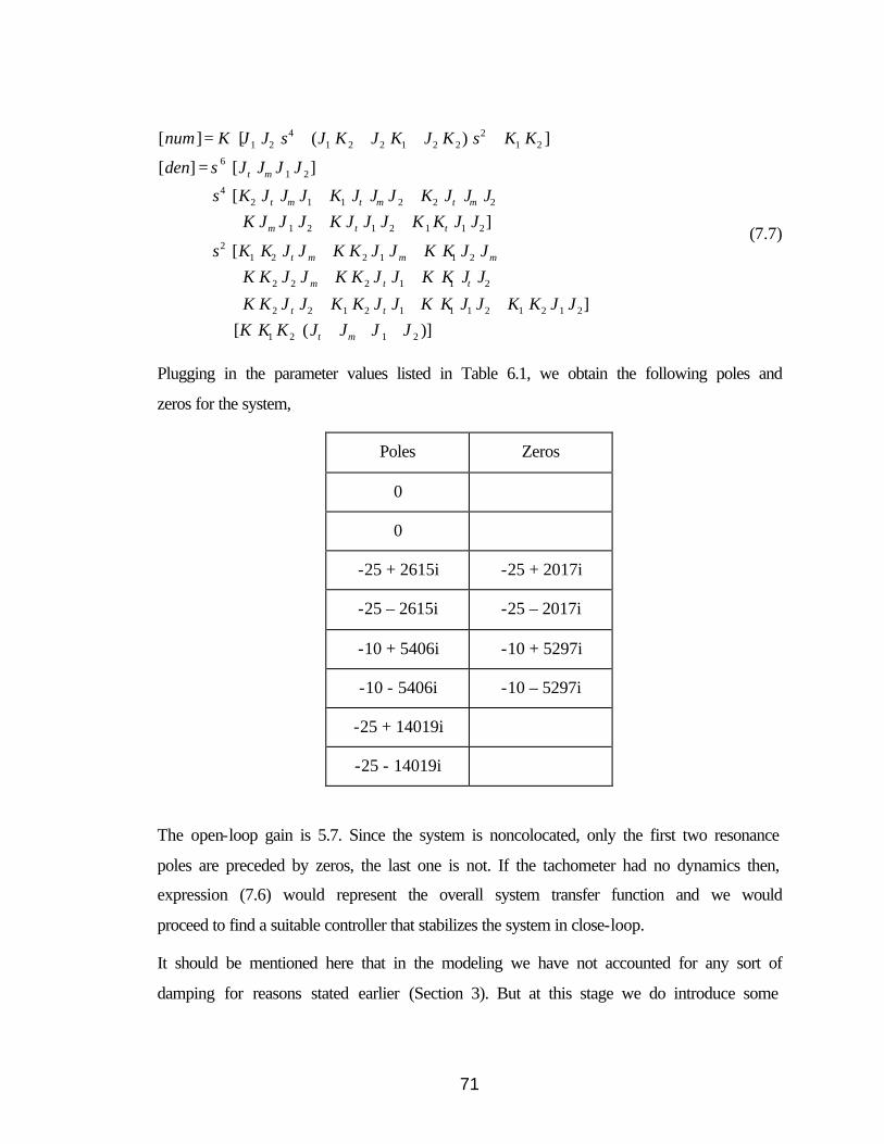
71

4 2 1 2 1 2 2 1 2 2 1 2

6 1 2

4 2 1 1 2 2 2

1 2 1 2 1 1 2

2 1 2

[ ] [ ( ) ]

[ ] [ ]

[ ]

[

t m

t m t m t m

m t t

t

num K J J s J K J K J K s K K

den s J J J J

s K J J J K J J J K J J JK J J J K J J J K K J J

s K K J

= + + + +

= +

+ + ++ + +

2 1 1 2

2 2 2 1 1 2

2 2 1 2 1 1 1 2 1 2 1 2

1 2 1 2

] [ ( )]

m m m

m t t

t t

t m

J K K J J K K J JK K J J K K J J K K J J

K K J J K K J J K K J J K K J JK K K J J J J

+ ++ +

+ + ++ + + +

(7.7)

Plugging in the parameter values listed in Table 6.1, we obtain the following poles and

zeros for the system,

Poles Zeros

0

0

-25 + 2615i -25 + 2017i

-25 – 2615i -25 – 2017i

-10 + 5406i -10 + 5297i

-10 - 5406i -10 – 5297i

-25 + 14019i

-25 - 14019i

The open-loop gain is 5.7. Since the system is noncolocated, only the first two resonance

poles are preceded by zeros, the last one is not. If the tachometer had no dynamics then,

expression (7.6) would represent the overall system transfer function and we would

proceed to find a suitable controller that stabilizes the system in close-loop.

It should be mentioned here that in the modeling we have not accounted for any sort of

damping for reasons stated earlier (Section 3). But at this stage we do introduce some

72

empirical values of damping at each of these poles and zeros to avoid singularities in the

root-locus and bode plots. These damping values are estimated by matching the

experimental frequency plots with the analytically predicted ones.

The actual root-locus for the open-loop system is as follows:

-500 -400 -300 -200 -100 0 100 200 300 400 500-1.5

-1

-0.5

0

0.5

1

1.5x 10

4

Real Axis

Imag

Axi

s

Fig. 7.17(a) t

mTθ

: Root-locus for the tachometer-motor-load mechanical system

For ease of visualization, the following exaggerated (yet qualitatively correct) plot (Fig

7.18(a)) of the same system. This provides a better picture of the pole and zero locations.

Clearly the system is marginally stable in close-loop. In Fig. 7.18(b), we investigate how

and to what extent can a lead controller help stabilize this system.

73

Fig. 7.18 Root locus for (a) Uncompensated system (b) Lead compensated system

74

Frequency (rad/sec)

Pha

se (

deg)

; Mag

nitu

de (

dB)

10-1 100 101 102 103 104 105-400

-200

0

200

-200

-100

0

100

Fig 7.19 Bode Plots for the system with lead compensation

As expected, since the system is noncolocated, a lead compensator does not make sure

that all the root-loci branches are on the left-hand side of the s-plane. Depending on the

lead zero location, the root-locus can take various forms but there are two braches

emanating from the last poles that always spill into the right-hand side. Nevertheless, it is

interesting to note that since the pole and-zero frequencies are so high and because there

is some damping present at the poles, we can get a reasonable closed-loop bandwidth

without destabilizing the system. Since the poles lie so far out on the frequency scale, the

open-loop gain can be increased still maintaining acceptable phase and gain margins. In

the particular case illustrated in the bode plots above, a crossover frequency of 100

rad/sec is achieved using the following lead controller,

15200

1500s

s+

+

This may or may not meet the desired rise time specifications. To achieve an even higher

bandwidth without causing the system to go unstable, it may be advisable to use a notch

75

compensator or a state-space controller (as was discussed in Section 7.2.3). It is also

noteworthy that the settling time is dependent on the first pole-zero pair location, since

the corresponding close-loop pole will lie close to this pole-zero pair.

But, we have to step back and realize that the tachometer does not act as a pure gain; it

adds sensor dynamics to the system. The fact that the tachometer reshuffles the original

zeros of the system and adds further zeros to the overall transfer function changes the

scenario completely. Referring back to Section 6, the overall transfer function with the

tachometer dynamics included is given by

2 [ ( ) ( ) ( )]

( )amp m r t tachtach

in

K K s den K s den K K numVV s den

− += (7.8)

where (num) and (den) are the same as defined in expression(7.7)

Referring to Section 5 of this thesis, we know that the tachometer dynamics causes the

system to have as many zeros as are the number of poles (including the pair at the origin).

If there are four pairs of complex conjugate poles (and if Km is positive, which it is for

this particular set-up) then there will be 4 complex-conjugate zeros in the overall system

transfer function. Since the system is no longer a purely mechanical but is now

electromechanical in nature, the alternating sequence of poles and zeros on the imaginary

axis is not assured. In fact we do observe the previously discussed phenomenon of pole-

zero flipping in this case. Furthermore, some of these new zeros lie on the right-hand side

of the s-plane making the system non-minimum phase and thus making the control

system design much more difficult. Now the zeros no longer add phase to the system,

they rather reduce phase from the system, which is a very unhealthy development.

Thus we notice that the tachometer dynamics complicates the matters to quite an extent.

We will see that while it was relatively easy to get an acceptable bandwidth had there

been no tachometer dynamics, in a real world case, the presence of tachometer dynamics

severely limits the controller capability. The following block diagram presents a

schematic of the overall open-loop system.

76

Motor

current (Im)

Torque Constant (Kt)

Kamp

Voltage to current amplifier

Vtach Tachometer

Output Voltage

Tach speed

Motor Current Tach voltage

Tachometer

Motor Torque Tach Speed

Tach-motor-load Mechanical System

Kt

Motor Model

Vin Input Voltage

Fig 7.20 Block-diagram based representation of the open-loop tachometer-motor-

load mechanical and electrical system

All the blocks inside the dotted square can be combined into one tachometer-motor-load

system that includes both the mechanical as well as electromagnetic model of the entire

system.

Motor

current (Im)

G(s)H(s)

Kamp

Voltage to current amplifier

Vtach Tachometer

Output Voltage

Motor Current Tach Voltage

Tach-Motor-Load Electromechanical System

Vin Input Voltage

Fig. 7.21 The tachometer-motor-load electromechanical system

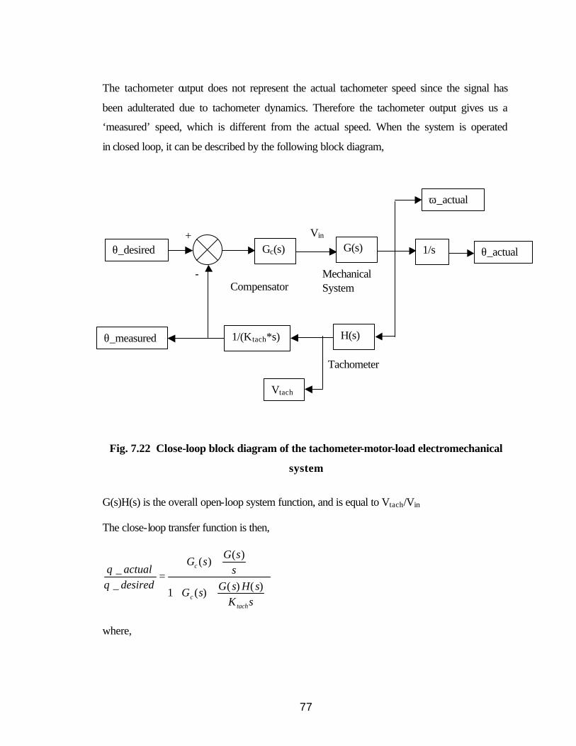
77

The tachometer output does not represent the actual tachometer speed since the signal has

been adulterated due to tachometer dynamics. Therefore the tachometer output gives us a

‘measured’ speed, which is different from the actual speed. When the system is operated

in closed loop, it can be described by the following block diagram,

Fig. 7.22 Close-loop block diagram of the tachometer-motor-load electromechanical

system

G(s)H(s) is the overall open-loop system function, and is equal to Vtach/Vin

The close-loop transfer function is then,

( )( )

__ ( ) ( )1 ( )

c

ctach

G sG s

actual sdesired G s H sG s

K s

θθ

=

+

where,

Compensator

Tachometer

-

+ θ_desired Gc(s) G(s)

H(s)

Mechanical System

1/s θ_actual

1/(Ktach*s) θ_measured

ω_actual

Vtach

Vin

78

2

2

[ ( ) ( ) ( )]( ) ( ) ( )

amp m r t tachtach

in

K K s den K s den K K numVG s H ss s V s den

− += =

Plugging the parameter values listed in Table 6.1, this open-loop transfer function yields

the following open-loop poles and zeros. The open-loop gain is 58.

Poles Zeros

0 118.5 + 1060i

0 118.5 – 1060i

-25 + 2615i 31.8 + 2814i

-25 – 2615i 31.8 - 2814i

-10 + 5406i 2 + 5419i

-10 - 5406i 2 - 5419i

-25 + 14019i -2.3 + 13934i

-25 - 14019i -2.3 - 13934i

Figures 23(a) and 23(b) provide the root-locus and Bode plots respectively for the

uncompensated tachometer-motor-load electromechanical system, with the new

tachometer model incorporated.

79

-200 -150 -100 -50 0 50 100 150 200-1.5

-1

-0.5

0

0.5

1

1.5x 10

4

Real Axis

Imag

Axi

s

Frequency (rad/sec)

Pha

se (

deg)

; Mag

nitu

de (

dB)

-150

-100

-50

0

101 102 103 104 105-1000

-800

-600

-400

-200

0

Fig. 7.23 (a) Root-locus plot (b) Bode plots for the uncompensated system

80

Because of the open-loop zeros on the right hand side of the plane the uncompensated

system is always unstable in close-loop for however low gains. From the bode plots it is

evident that the phase margin approaches zero for low gains but is never positive. The

fact that there is pole-zero flipping doesn’t have too much of an influence since the pole

and zero are very closely placed.

Next we investigate the influence of a lead controller on the stability of the system.

-200 -150 -100 -50 0 50 100 150 200-1.5

-1

-0.5

0

0.5

1

1.5x 10

4

Real Axis

Imag

Axi

s


electromechanical system

81

Frequency (rad/sec)

Pha

se (

deg)

; Mag

nitu

de (

dB)

10-1 100 101 102 103 104 105-1000

-500

0

-200

-100

0

100

200

Fig. 7.24(b) Bode plots for the lead compensated tachometer-motor-load

electromechanical system

These plots reveal some interesting information. The root-locus plots tells us that the

system is close-loop stable only up till a certain value of gain, beyond which the root loci

branches spill over into the right-hand side of the s-plane. This is confirmed from the

Bode plots. The crossover frequency can be raised only to a certain extent, by increasing

the gain, beyond which the phase margin becomes negative. Since this is a non-minimum

phase system, it is phase-deficient and hence the simple lead compensator is only of

limited help. Nevertheless, a bandwidth of approximately 200rad/sec is realizable as

shown in the above case, using the following lead compensator,

620

185s

s+

+

Once again, the settling time is limited by the location of the closest pole-zero pair, as

was explained earlier. One influence of the tachometer on the open-loop system is that it

82

brings the smallest zero closer to the origin. Consequently, the resulting close-loop pole

is closer to the origin, thereby increasing the settling time marginally. Overall the

tachometer dynamics has a deteriorating effect on the close-loop performance of the

tachometer-motor-load system. To achieve better time-response characteristics, it is

essential to look into other possible controller designs. Clearly a notch-filter is of no use

in this case. The possibility of using a state-space controller can be explored.

83

8. CONCLUDING REMARKS AND FUTURE WORK

The conventional DC tachometer model was found to be inadequate for predicting the

high-frequency responses, in cases when the tachometer is integrated with a DC motor.

This led to the investigation of a more accurate tachometer model. Based on fundamental

principles of electromagnetism, a new tachometer model was derived that includes the

effects of mutual inductance between motor and tachometer windings, and the loading of

the tachometer. In the high frequency domain, the tachometer can no longer be treated as

a simple gain; it introduces some additional zeros in the feedback path. This leads to

interesting consequences that are described in this thesis.

It is shown that, if high-speed servo-control is desired, the tachometer dynamics can play

a significant role in the control system design. Since the tachometer-motor-load system is

a multiple inertia system with multiple flexible elements, the concepts of colocated and

noncolocated controls are revisited. The physical interpretation of poles and zeros in

colocated and noncolocated transfer functions are sought using a simple system. These

concepts are then extended to the case at hand. Once the mechanical system has been

understood, the influence of tachometer dynamics on the overall system is discussed. The

tachometer dynamics makes the system non-minimum phase, which makes the control-

system design more complicated. It is found that the tachometer dynamics limits the

performance of the close-loop system when lead controller is used. The bandwidth of the

overall system cannot be increased beyond a certain limit without risking the system

stability.

For future work, it is a very good exercise to design a robust state-space controller for

this system that may allow for better a time-domain performance. Also it would be very

instructive to build an experimental multiple-mass and multiple-spring system (preferably

a four-mass three-spring system). This would be of much help in developing a physical

understanding of poles and zeros of such a system. Without an actual experimental test-

bed, it is difficult to visualize the various resonance modes for such a system, since a

resonance mode in general involves resonance in more than one spring.

84

With reference to new tachometer model, some observations that are not modeled are

also presented. A slight droop observed in the experimental phase plot may be due to

dead time effect towards the higher frequency range. This effect is not included in the

model.

Also, we have not accounted for any dynamics associated with the drive circuitry

including servo amplifier. We developed the system model assuming that the drive

circuitry has infinite bandwidth. A comparison of the predictions of this model with the

experimental results showed little discrepancy. Based on this, we concluded that for the

frequency range over which we are testing the system, the assumption regarding the

driver dynamics is acceptable. The slight droop in the phase plot, mentioned earlier, may

be due to a small delay time associated with the drive circuit.

During the derivation of system transfer functions, we have neglected mechanical

damping. This is justified by the argument that mechanical damping does not affect the

existence of system poles and zeros; it only reduces their intensity.

The purpose of this research was to point out an important electromagnetic phenomenon,

which shouldn’t be neglected without due consideration. It can significantly affect the

system performance. The tachometer dynamics is certainly not negligible because the

first tachometer-induced zero occurs much before the first system pole. But, the

tachometer dynamics identified in this thesis is extremely sensitive because Km and Kr

can vary from case to case and this change can significantly alter the high-frequency

system dynamics.

85

REFERENCES

1. Fitzgerald, A.E. and Kingsley, C., 1961, Electric Machinery: The Dynamics and

Statics of Electromechanical Energy Conversion, McGraw-Hill Book Company.

2. Sen, P.C., 1989, Principles of Electric Machines and Power Electronics, John

Wiley & Sons.

3. McLean, D., 1978, “Mathematical Models of Electrical Machines,” Measurement

and Control, Vol. 11, June, pp. 231-236.

4. Welch Jr., R.H., “Mechanical Resonance in a Closed Loop Servo System”,

Tutorial for Motion Control Expo.

5. Ogata, K., 1998, Modern Control Engineering, Prentice-Hall

6. Cannon, R.H. Jr., and Rosenthal, D.E., 1984, “Experiments in Control of Flexible

Structures with Noncolocated Sensors and Actuators,” Journal of Guidance,

Vol.7, No.5, Oct., pp. 546-553.

7. Miu, D.K., 1991, “Physical Interpretation of Transfer Functions Zeros for Simple

Control Systems With Mechanical Flexibilities,” ASME Journal of Dynamics

Systems, Measurement and Control, Vol.113, Sept., pp. 419-424.

8. Spector, V., and Flashner, H., 1990, “Modeling and Design Implications of

Noncolocated Control in Flexible Systems,” ASME Journal of Dynamics Systems,

Measurement and Control, Vol.112, June, pp. 186-163.

9. Friedland, B., 1996, Advanced Control System Design, Prentice-Hall

10. Franklin, G.F. and Powell, J.D., 1994, Feedback Control of Dynamic Systems,

Addison-Wesley Publishing Company

Documents

MAGNETIC COUPLING BETWEEN DC TACHOMETER AND