Embed Size (px)
Citation preview
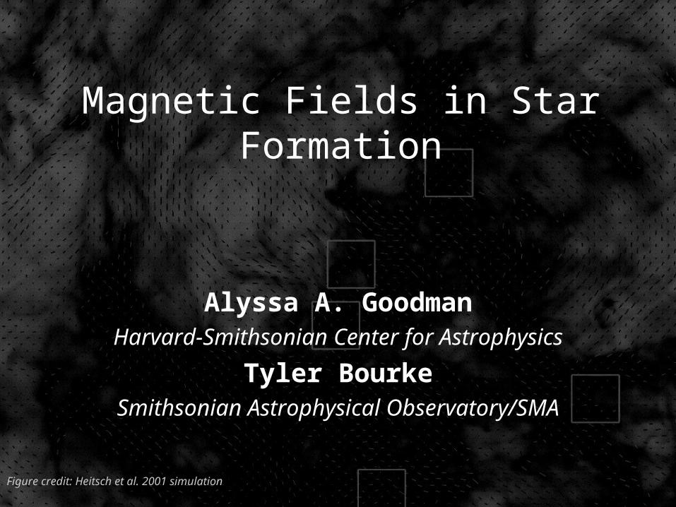
Magnetic Fields in Star Formation
Alyssa A. GoodmanHarvard-Smithsonian Center for
Astrophysics
Tyler BourkeSmithsonian Astrophysical
Observatory/SMAFigure credit: Heitsch et al. 2001 simulation
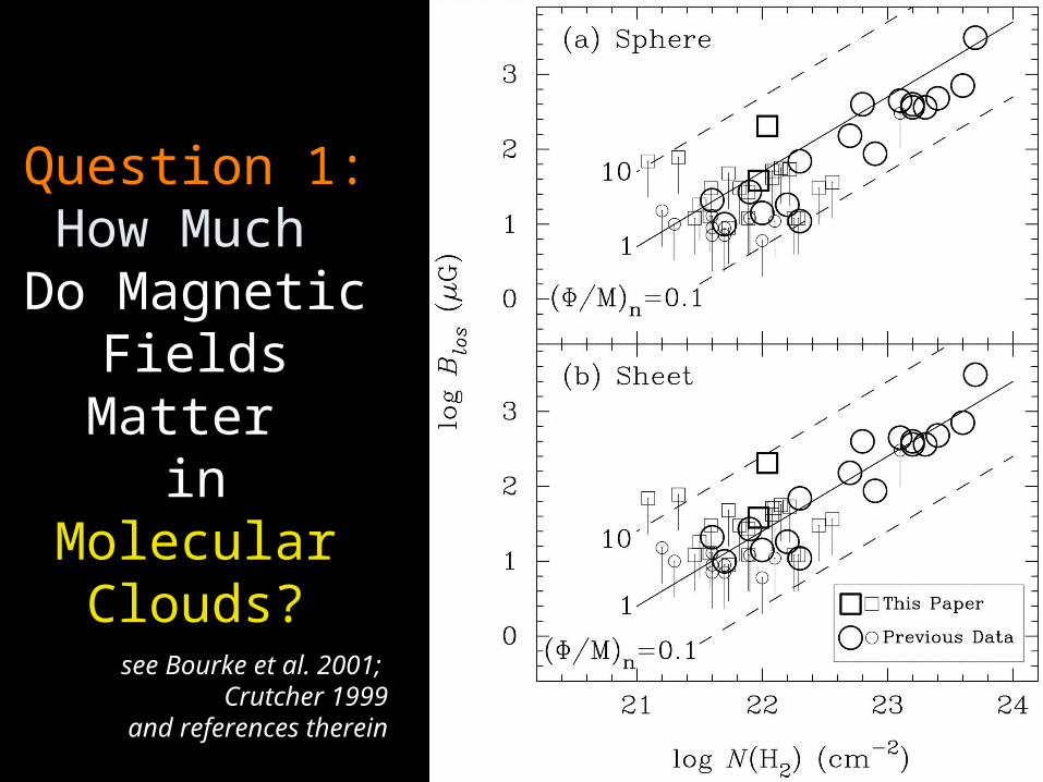
Question 1:How Much
Do Magnetic Fields Matter in Molecular
Clouds?
see Bourke et al. 2001; Crutcher 1999
and references therein
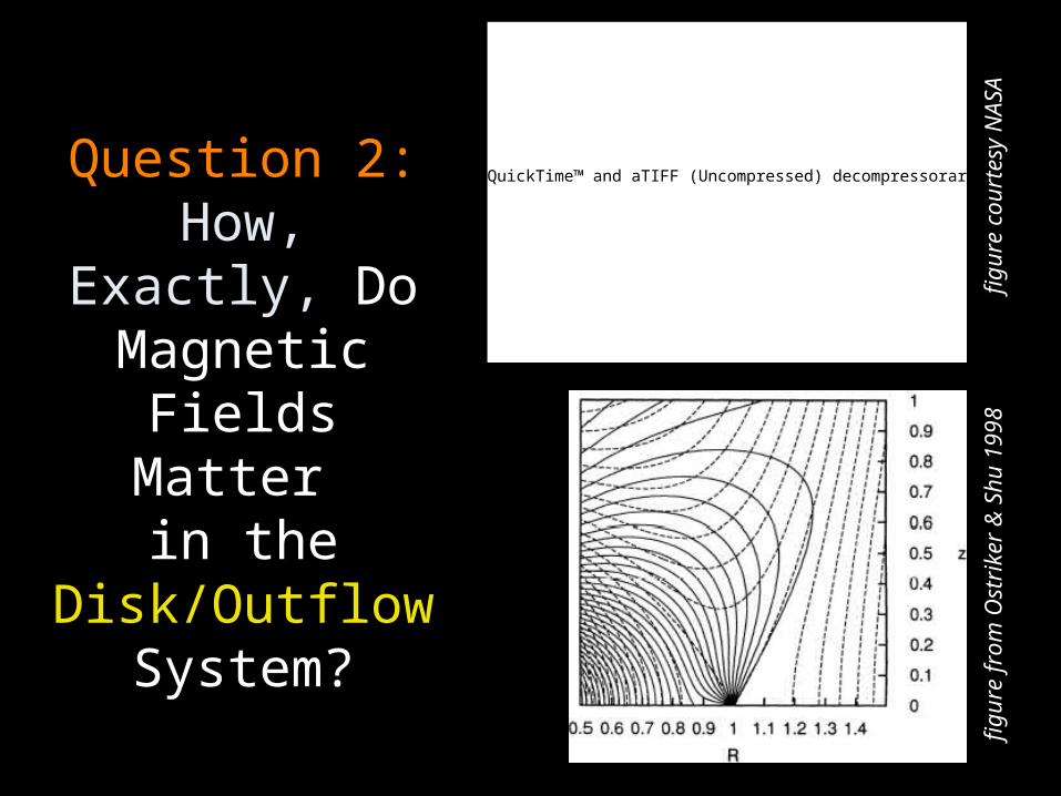
Question 2:How, Exactly, Do Magnetic Fields Matter
in the Disk/Outflow
System?
figure
fro
m O
stri
ker
& S
hu 1
99
8
QuickTime™ and aTIFF (Uncompressed) decompressorare needed to see this picture.
figure
court
esy
NA
SA
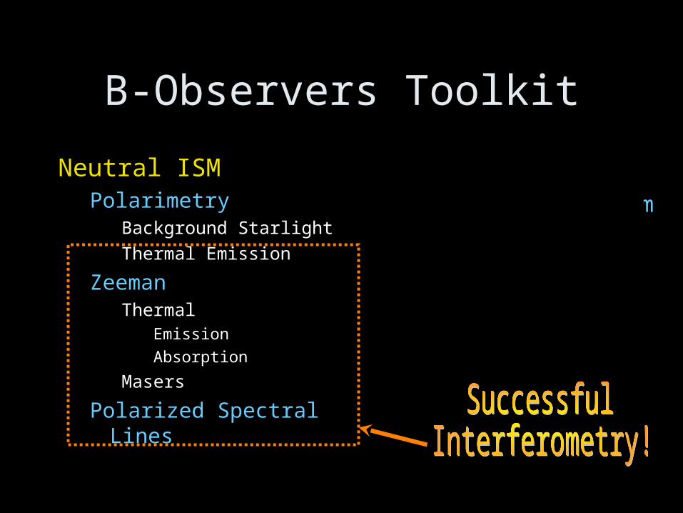
B-Observers Toolkit
Neutral ISMPolarimetry
Background Starlight
Thermal Emission
ZeemanThermal
EmissionAbsorption
Masers
Polarized Spectral Lines
Ionized ISMPolarized continuum
B directionFaraday Rotation
B=RM/DM
Recombination Line Masers
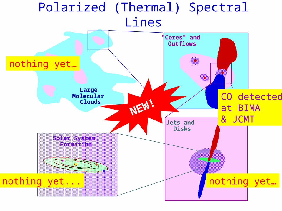
Large Molecular
Clouds
Jets and Disks
"Cores" and Outflows
Solar System Formation
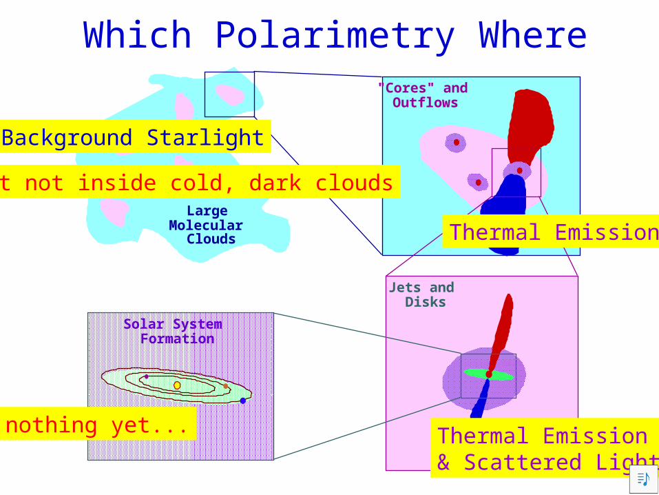
Which Polarimetry Where
Background Starlight
nothing yet...
Thermal Emission
Thermal Emission& Scattered Light
but not inside cold, dark clouds
Large Molecular
Clouds
Jets and Disks
"Cores" and Outflows
Solar System Formation
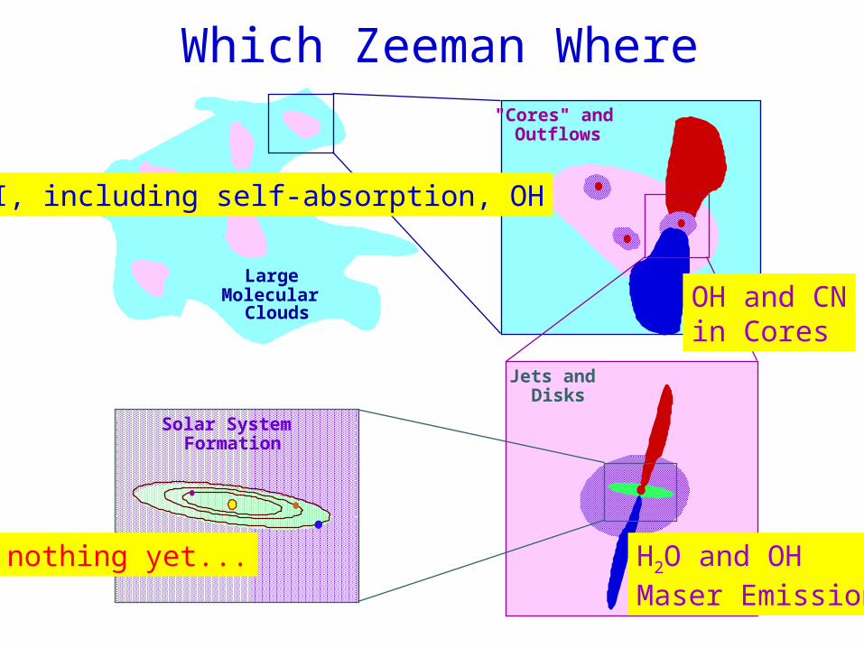
Which Zeeman Where
H I, including self-absorption, OH
nothing yet...
OH and CNin Cores
H2O and OHMaser Emission
Large Molecular
Clouds
Jets and Disks
"Cores" and Outflows
Solar System Formation
Polarized (Thermal) Spectral Lines
CO detectedat BIMA & JCMT
nothing yet…
nothing yet... nothing yet…
NEW!
B-Analysis Toolkit
Analytic Predictions
Numerical Simulations
Chandrasekhar-Fermi Method
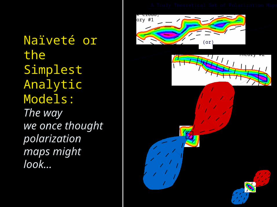
Naïveté or the Simplest Analytic Models:The waywe once thoughtpolarization maps might look…
(or)
Disk + Star
Core
Dark Cloud, Theory #2
Dark Cloud, Theory #1
A Truly Theoretical Set of Polarization Maps
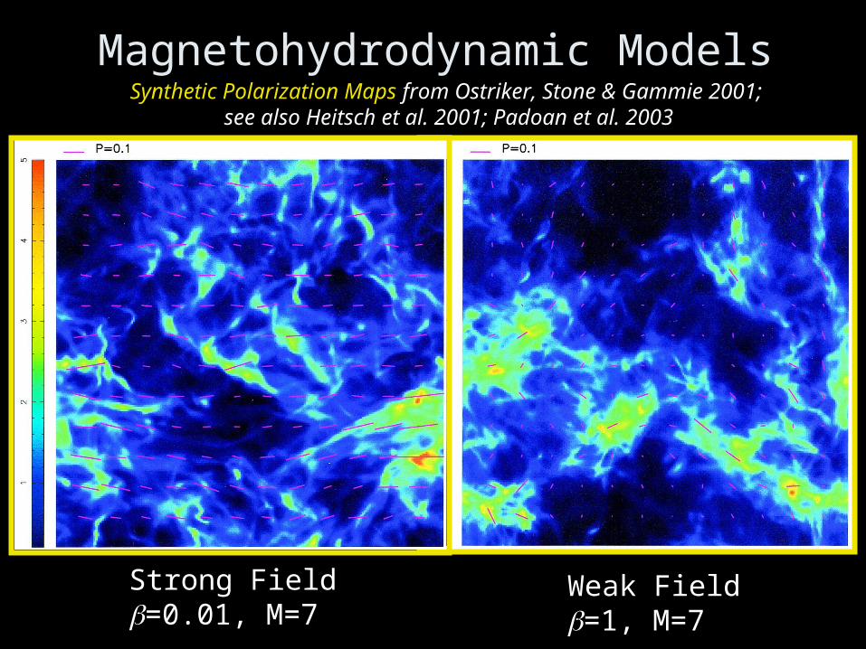
Magnetohydrodynamic Models
Strong Field=0.01, M=7
Weak Field=1, M=7
Synthetic Polarization Maps from Ostriker, Stone & Gammie 2001; see also Heitsch et al. 2001; Padoan et al. 2003
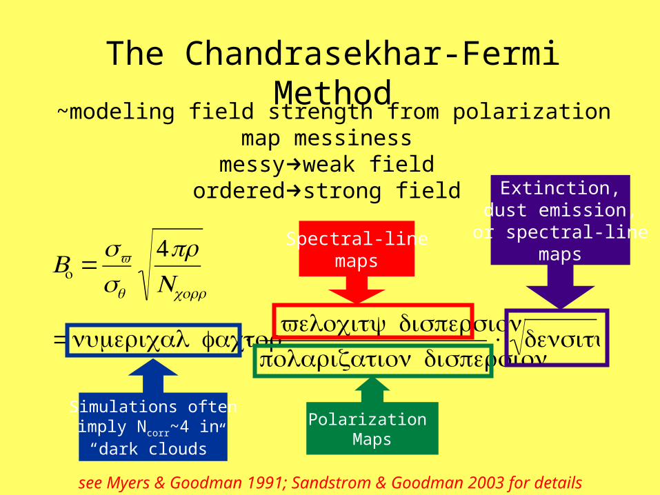
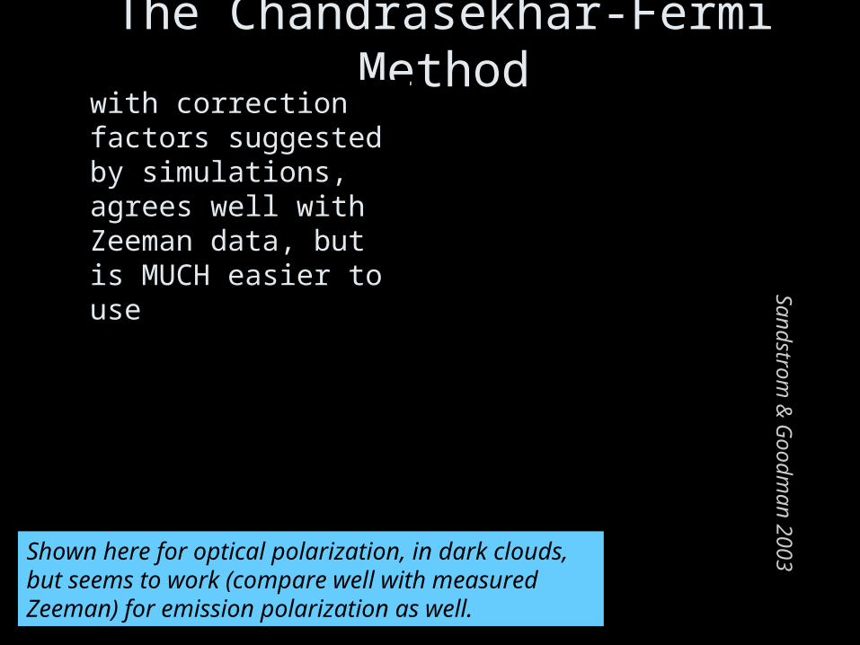
The Chandrasekhar-Fermi Method
€
Bo =σv
σθ
4πρNcorr
= numerical factor× velocity dispersion
polarization dispersion× density
see Myers & Goodman 1991; Sandstrom & Goodman 2003 for details
~modeling field strength from polarization map messiness
messyweak fieldorderedstrong field
Simulations oftenimply Ncorr~4 in “dark clouds”
Polarization Maps
Spectral-linemaps
Extinction,dust emission,or spectral-line
maps
B-Observers Toolkit
Neutral ISMPolarimetry
Background Starlight
Thermal Emission
ZeemanThermal
EmissionAbsorption
Masers
Polarized Spectral Lines
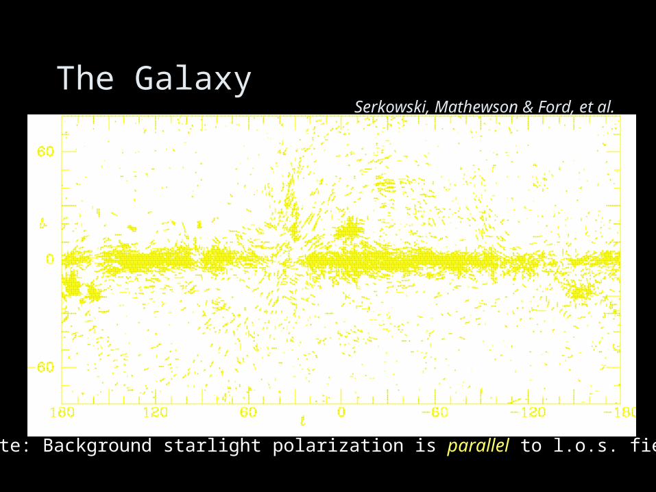
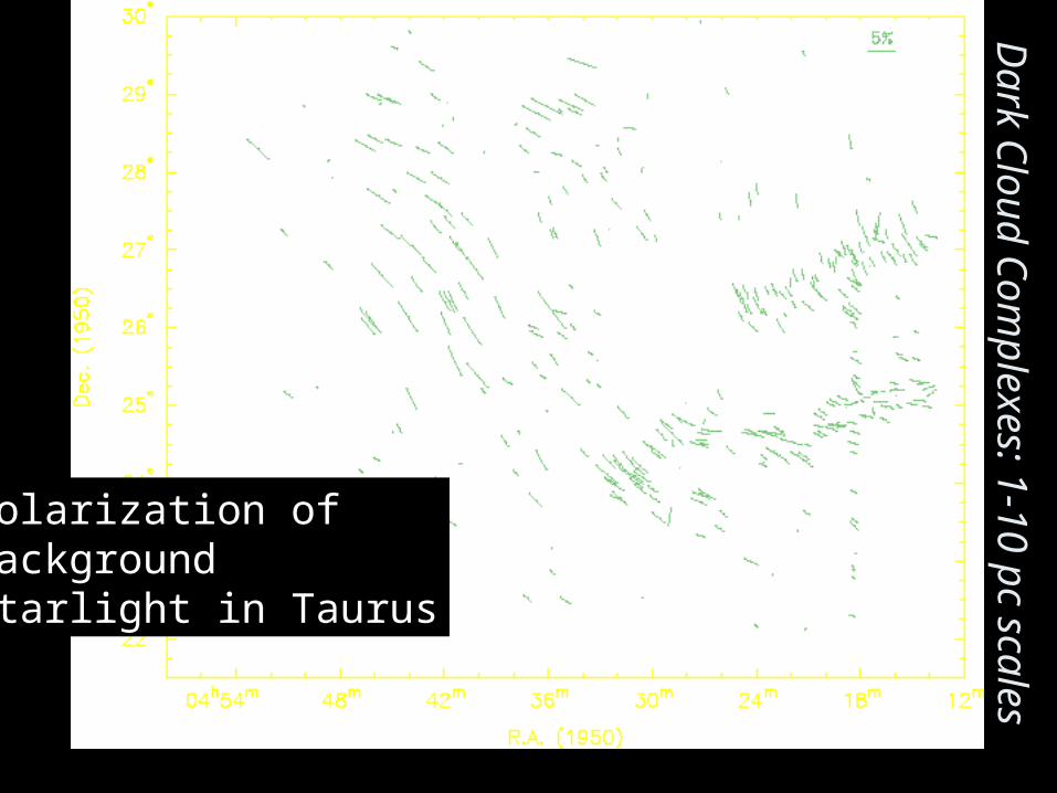
The GalaxyThe GalaxySerkowski, Mathewson & Ford, et al.
Note: Background starlight polarization is parallel to l.o.s. field
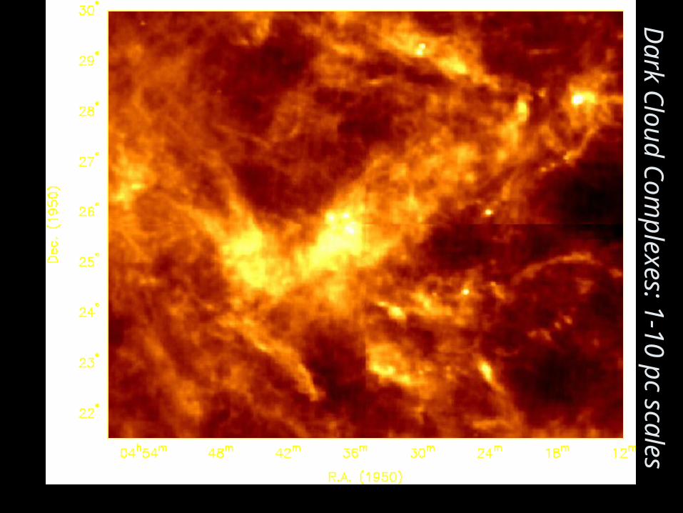
Dark C
loud
Com
ple
xes: 1
-10 p
c sca
les
Dark C
loud
Com
ple
xes: 1
-10 p
c sca
les
Polarization ofBackground Starlight in Taurus
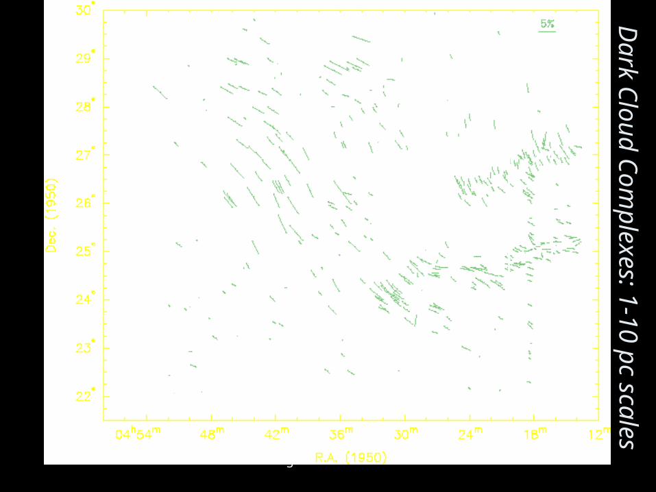
Magnetic Fields
Dark C
loud
Com
ple
xes: 1
-10 p
c sca
les
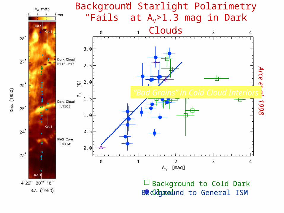
Background Starlight Polarimetry “Fails” at AV>1.3 mag in Dark Clouds
3.0
2.5
2.0
1.5
1.0
0.5
0.0
PR
[%]
43210
43210AV [mag]
Background to Cold Dark Cloud
Arce
et a
l. 1998
Background to General ISMcf. Goodman et al. 1992; 1995
“Bad Grains” in Cold Cloud Interiors
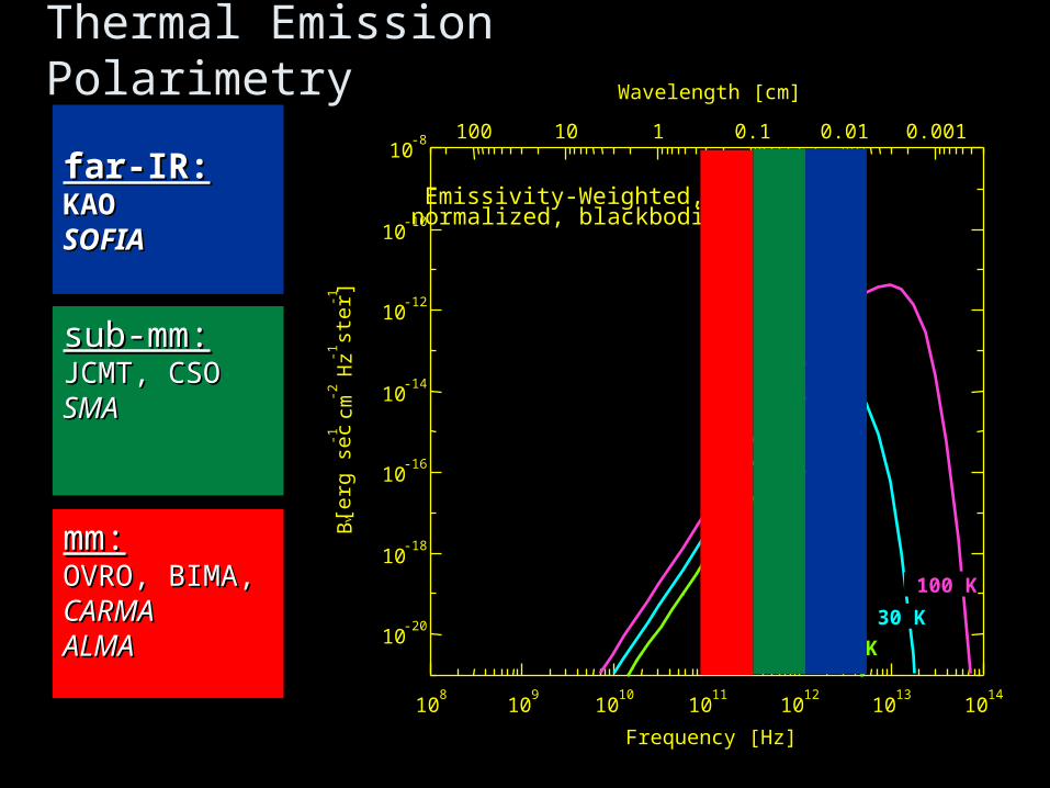
Thermal Emission Polarimetry
10-20
10-18
10-16
10-14
10-12
10-10
10-8
B [
erg
sec-1
cm
-2 H
z-1 s
ter-1
]
0.0010.010.1110100
Wavelength [cm]
108
109
1010
1011
1012
1013
1014
Frequency [Hz]
Emissivity-Weighted, normalized, blackbodies
10 K
30 K
100 K
sub-mm:sub-mm:JCMT, CSOJCMT, CSOSMASMA
far-IR:far-IR:KAOKAOSOFIASOFIA
mm:mm:OVRO, BIMA, OVRO, BIMA, CARMACARMAALMAALMA
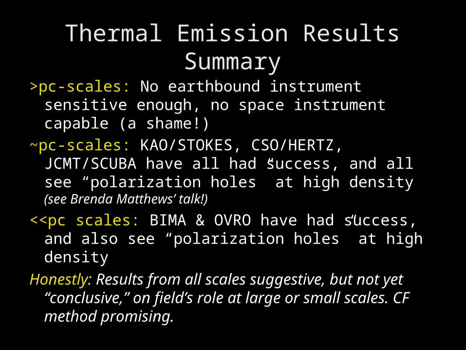
Thermal Emission Results Summary
>pc-scales: No earthbound instrument sensitive enough, no space instrument capable (a shame!)
~pc-scales: KAO/STOKES, CSO/HERTZ, JCMT/SCUBA have all had success, and all see “polarization holes” at high density (see Brenda Matthews’ talk!)
<<pc scales: BIMA & OVRO have had success, and also see “polarization holes” at high density
Honestly: Results from all scales suggestive, but not yet “conclusive,” on field’s role at large or small scales. CF method promising.
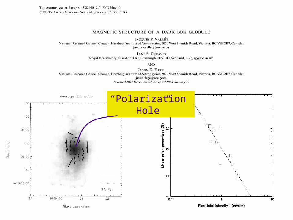
Vallé et al. 2003
“Polarization Hole”
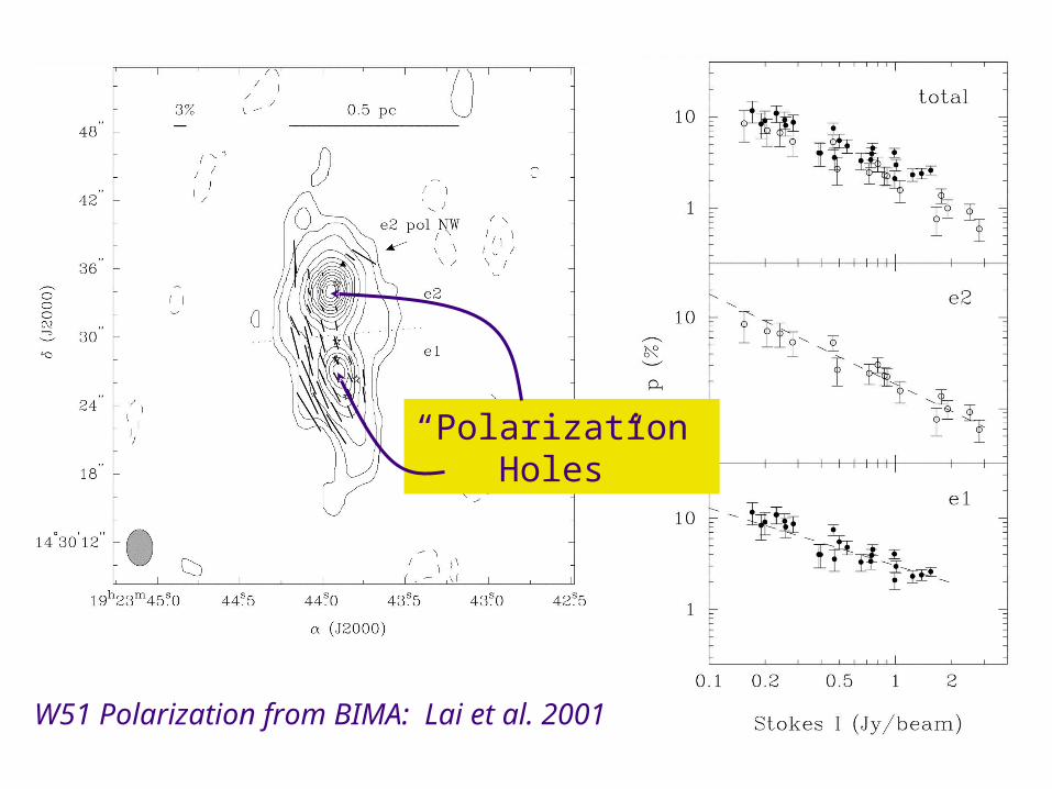
W51 Polarization from BIMA: Lai et al. 2001
“Polarization Holes”
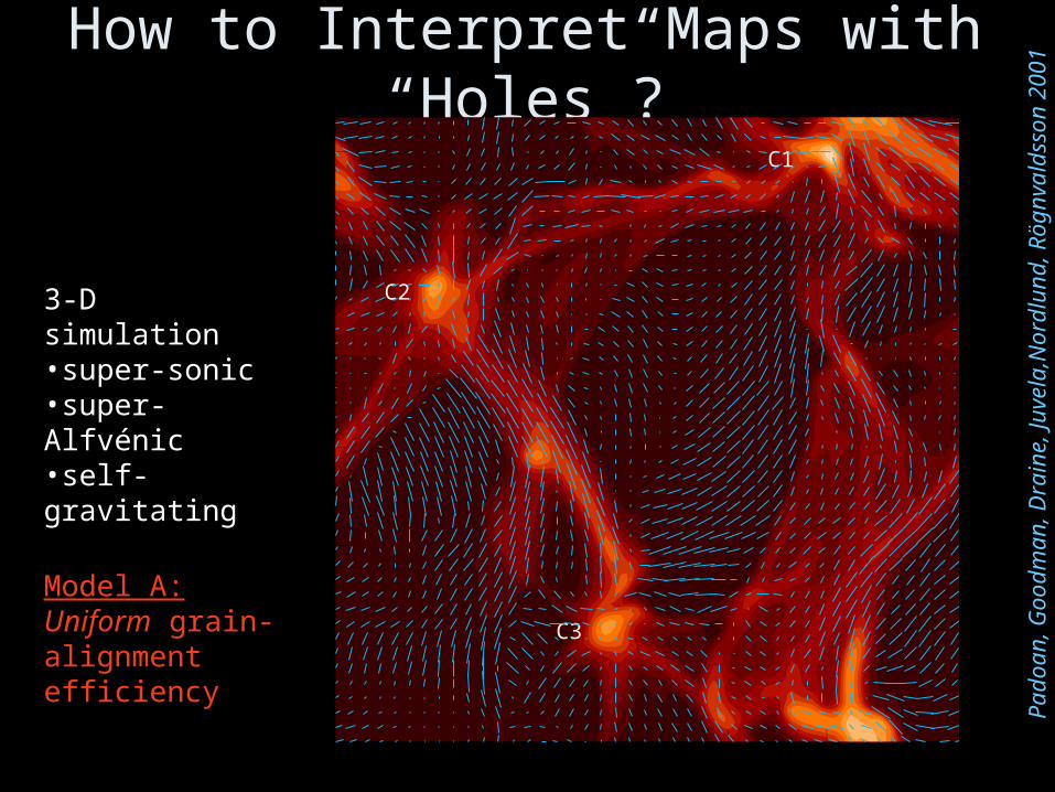
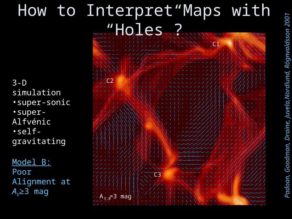
How to Interpret Maps with “Holes”?
C2
C3
C1
Padoan, G
oodm
an, D
rain
e, Ju
vela
,Nord
lund, R
ögnvald
sson 2
00
1
3-D simulation•super-sonic•super-Alfvénic•self-gravitating
Model A:Uniform grain-alignment efficiency
Padoan, G
oodm
an, D
rain
e, Ju
vela
,Nord
lund, R
ögnvald
sson 2
00
1
3-D simulation•super-sonic•super-Alfvénic•self-gravitating
Model B:Poor Alignment at AV≥3 mag
C2
C3
C1
AV,0 =3 mag
How to Interpret Maps with “Holes”?
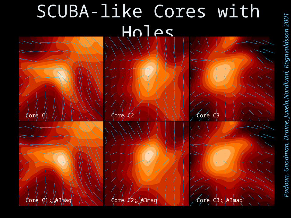
SCUBA-like Cores with Holes
Core C1
Core C2
Core C3
Core C1; AV,0=3 mag
Core C2; AV,0=3 mag
Core C3; AV,0=3 mag
Padoan, G
oodm
an, D
rain
e, Ju
vela
,Nord
lund, R
ögnvald
sson 2
00
1
It seems nearly all polarization maps show decrease in polarizing efficiency with density.
Derived models of 3D field (for comparisons) need to
take this into account.
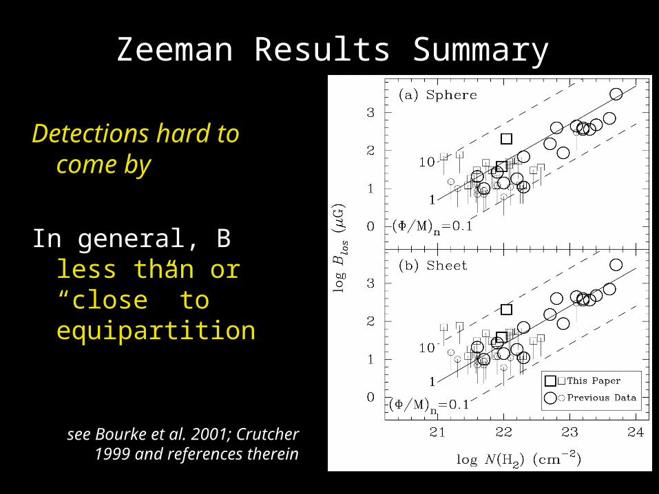
Zeeman Results Summary
see Bourke et al. 2001; Crutcher 1999 and references
therein
Detections hard to come by
In general, B less than or “close” to equipartition
The Chandrasekhar-Fermi Method
with correction factors suggested by simulations, agrees well with Zeeman data, but is MUCH easier to use S
andstro
m &
Goodm
an
2003
Shown here for optical polarization, in dark clouds,but seems to work (compare well with measured Zeeman) for emission polarization as well.
Polarized Spectral-Line Summary
Effect predicted by Goldreich & Kylafis, 1981
1st detection in a star-forming region (NGC 1333): Girart et al. 1999 (BIMA)
Subsequent detection with JCMT/SCUBA (in NGC2024): Greaves et al. 2001
Still very difficult to interpret (polarization can be parallel or perpendicular to B!--need context)
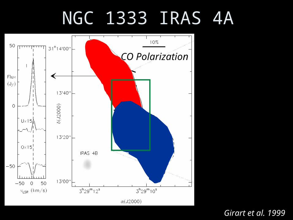
NGC 1333 IRAS 4A
Girart et al. 1999
CO Polarization
Dust Polarization(in white)
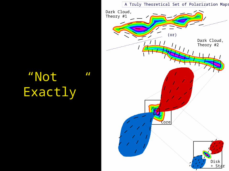
“Not ,Exactly”
(or)
Disk + Star
Core
Dark Cloud, Theory #2
Dark Cloud, Theory #1
A Truly Theoretical Set of Polarization Maps
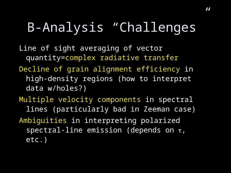
B-Analysis “Challenges”
Line of sight averaging of vector quantity=complex radiative transfer
Decline of grain alignment efficiency in high-density regions (how to interpret data w/holes?)
Multiple velocity components in spectral lines (particularly bad in Zeeman case)
Ambiguities in interpreting polarized spectral-line emission (depends on , etc.)
Question 1:How Much
Do Magnetic Fields Matter in Molecular Clouds?
Question 2:How, Exactly, Do Magnetic
Fields Matter in the Disk/Outflow System?
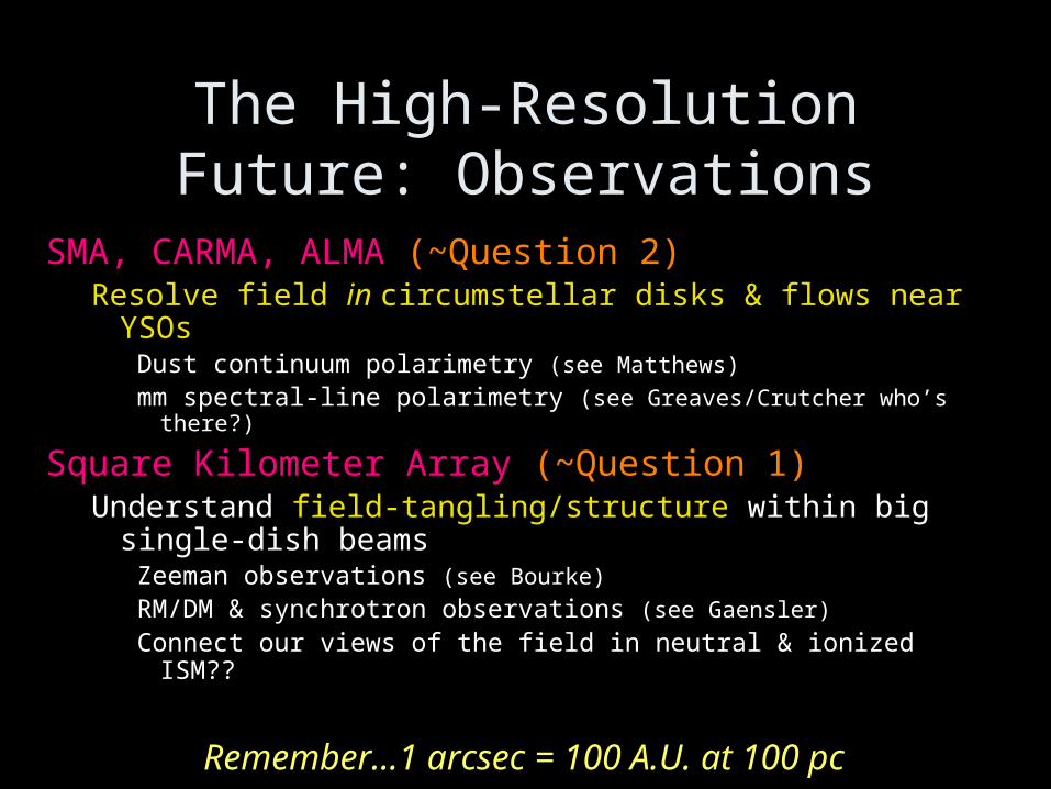
The High-Resolution Future: Observations
SMA, CARMA, ALMA (~Question 2)Resolve field in circumstellar disks & flows near
YSOs Dust continuum polarimetry (see Matthews)
mm spectral-line polarimetry (see Greaves/Crutcher who’s there?)
Square Kilometer Array (~Question 1)Understand field-tangling/structure within big
single-dish beamsZeeman observations (see Bourke)
RM/DM & synchrotron observations (see Gaensler)
Connect our views of the field in neutral & ionized ISM??
Remember…1 arcsec = 100 A.U. at 100 pc
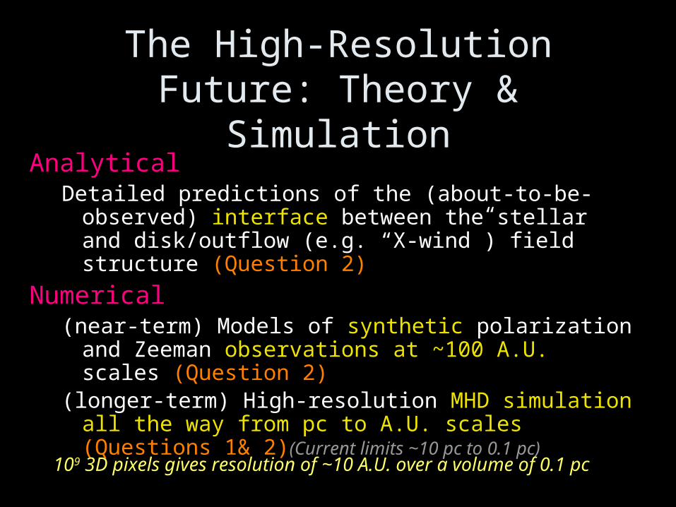
The High-Resolution Future: Theory & Simulation
AnalyticalDetailed predictions of the (about-to-be-observed)
interface between the stellar and disk/outflow (e.g. “X-wind”) field structure (Question 2)
Numerical(near-term) Models of synthetic polarization and
Zeeman observations at ~100 A.U. scales (Question 2)
(longer-term) High-resolution MHD simulation all the way from pc to A.U. scales (Questions 1& 2)(Current limits ~10 pc to 0.1 pc)
109 3D pixels gives resolution of ~10 A.U. over a volume of 0.1 pc
The Unconventional Future
Incorporating neutral/ion line width ratios to get 3D field (see Houdé et al. 2002)
Anisotropy in velocity centroid maps as a diagnostic of the mean magnetic field strength in cores (see Vestuto, Ostriker & Stone 2003)
Interpretation of microwave polarization (e.g. from WMAP) as due to rapidly spinning (magnetically aligned?) grains (see Finkbeiner 2003 and Hildebrand & Kirby 2003 & references therein)