arX

iv:1

805.

0613

1v2

[as

tro-

ph.G

A]

8 J

un 2

018

Draft version June 11, 2018

Typeset using LATEX twocolumn style in AASTeX61

MAGNETIC FIELDS TOWARDS OPHIUCHUS-B DERIVED FROM SCUBA-2 POLARIZATION

MEASUREMENTS

Archana Soam,1 Kate Pattle,2, 3, 4 Derek Ward-Thompson,2 Chang Won Lee,1, 5 Sarah Sadavoy,6

Patrick M. Koch,7 Gwanjeong Kim,1, 5, 8 Jungmi Kwon,9 Woojin Kwon,1, 5 Doris Arzoumanian,10 David Berry,11

Thiem Hoang,1, 5 Motohide Tamura,12, 13, 3 Sang-Sung Lee,1, 5 Tie Liu,1, 11 Kee-Tae Kim,1 Doug Johnstone,14, 15

Fumitaka Nakamura,16, 17 A-Ran Lyo,1 Takashi Onaka,12 Jongsoo Kim,1, 5 Ray S. Furuya,18, 19 Tetsuo Hasegawa,3

Shih-Ping Lai,4, 7 Pierre Bastien,20 Eun Jung Chung,1 Shinyoung Kim,1, 5 Harriet Parsons,11 Mark G. Rawlings,11

Steve Mairs,11 Sarah F. Graves,11 Jean-Franois Robitaille,21 Hong-Li Liu,22 Anthony P. Whitworth,23

Chakali Eswaraiah,4 Ramprasad Rao,7 Hyunju Yoo,24 Martin Houde,25 Ji-hyun Kang,26 Yasuo Doi,27

Minho Choi,1 Miju Kang,1 Simon Coude,20 Hua-bai Li,22 Masafumi Matsumura,28 Brenda C. Matthews,14, 15

Andy Pon,25 James Di Francesco,14, 15 Saeko S. Hayashi,29 Koji S. Kawabata,30, 31, 32 Shu-ichiro Inutsuka,10

Keping Qiu,33, 34 Erica Franzmann,35 Per Friberg,11 Jane S. Greaves,23 Jason M. Kirk,2 Di Li,36

Hiroko Shinnaga,37 Sven van Loo,38 Yusuke Aso,12 Do-Young Byun,26, 5 Huei-Ru Chen,4, 7 Mike C.-Y. Chen,15

Wen Ping Chen,39 Tao-Chung Ching,36, 40 Jungyeon Cho,24 Antonio Chrysostomou,41 Emily Drabek-Maunder,23

Stewart P. S. Eyres,2 Jason Fiege,35 Rachel K. Friesen,42 Gary Fuller,21 Tim Gledhill,41 Matt J. Griffin,23

Qilao Gu,22 Jennifer Hatchell,43 Wayne Holland,44, 45 Tsuyoshi Inoue,10 Kazunari Iwasaki,46 Il-Gyo Jeong,1

Sung-ju Kang,1 Francisca Kemper,7 Kyoung Hee Kim,47 Mi-Ryang Kim,1 Kevin M. Lacaille,48, 49

Jeong-Eun Lee,50 Dalei Li,51 Junhao Liu,33, 34 Sheng-Yuan Liu,7 Gerald H. Moriarty-Schieven,14

Hiroyuki Nakanishi,37 Nagayoshi Ohashi,29 Nicolas Peretto,23 Tae-Soo Pyo,29, 17 Lei Qian,40 Brendan Retter,23

John Richer,52, 53 Andrew Rigby,23 Giorgio Savini,54 Anna M. M. Scaife,21 Ya-Wen Tang,7 Kohji Tomisaka,16, 17

Hongchi Wang,55 Jia-Wei Wang,4 Hsi-Wei Yen,7, 56 Jinghua Yuan,40 Chuan-Peng Zhang,40 Guoyin Zhang,40

Jianjun Zhou,51 Lei Zhu,40 Philippe Andre,57 C. Darren Dowell,58 Sam Falle,59 Yusuke Tsukamoto,37

Yoshihiro Kanamori,27 Akimasa Kataoka,16 Masato I.N. Kobayashi,10 Tetsuya Nagata,60 Hiro Saito,61

Masumichi Seta,62 Jihye Hwang,1, 5 Ilseung Han,1, 5 Hyeseung Lee,24 and Tetsuya Zenko60

1Korea Astronomy and Space Science Institute, 776 Daedeokdae-ro, Yuseong-gu, Daejeon 34055, Republic of Korea2Jeremiah Horrocks Institute, University of Central Lancashire, Preston PR1 2HE, UK3National Astronomical Observatory of Japan, National Institutes of Natural Sciences, Osawa, Mitaka, Tokyo 181-8588, Japan4Institute of Astronomy and Department of Physics, National Tsing Hua University, Hsinchu 30013, Taiwan5Korea University of Science and Technology, 217 Gajang-ro, Yuseong-gu, Daejeon 34113, Korea6Harvard-Smithsonian Center for Astrophysics, 60 Garden Street, Cambridge, MA 02138, USA7Academia Sinica Institute of Astronomy and Astrophysics, P.O. Box 23-141, Taipei 10617, Taiwan8Nobeyama Radio Observatory (NRO), National Astronomical Observatory of Japan (NAOJ), Japan9Institute of Space and Astronautical Science, Japan Aerospace Exploration Agency, 3-1-1 Yoshinodai, Chuo-ku, Sagamihara, Kanagawa

252-5210, Japan10Department of Physics, Graduate School of Science, Nagoya University, Furo-cho, Chikusa-ku, Nagoya 464-8602, Japan11East Asian Observatory, 660 N. A‘ohoku Place, University Park, Hilo, HI 96720, USA12Department of Astronomy, Graduate School of Science, The University of Tokyo, 7-3-1 Hongo, Bunkyo-ku, Tokyo 113-0033, Japan13Astrobiology Center, National Institutes of Natural Sciences, 2-21-1 Osawa, Mitaka, Tokyo 181-8588, Japan14NRC Herzberg Astronomy and Astrophysics, 5071 West Saanich Road, Victoria, BC V9E 2E7, Canada15Department of Physics and Astronomy, University of Victoria, Victoria, BC V8P 1A1, Canada16Division of Theoretical Astronomy, National Astronomical Observatory of Japan, Mitaka, Tokyo 181-8588, Japan17SOKENDAI (The Graduate University for Advanced Studies), Hayama, Kanagawa 240-0193, Japan18Tokushima University, Minami Jousanajima-machi 1-1, Tokushima 770-8502, Japan19Institute of Liberal Arts and Sciences Tokushima University, Minami Jousanajima-machi 1-1, Tokushima 770-8502, Japan

Corresponding author: Archana Soam

archanasoam.bhu@gmail.com

2 Soam et al.

20Centre de recherche en astrophysique du Quebec & departement de physique, Universite de Montreal, C.P. 6128, Succ. Centre-ville,

Montreal, QC, H3C 3J7, Canada21Jodrell Bank Centre for Astrophysics, School of Physics and Astronomy, University of Manchester, Oxford Road, Manchester, M13 9PL,

UK22Department of Physics, The Chinese University of Hong Kong, Shatin, N.T., Hong Kong23School of Physics and Astronomy, Cardiff University, The Parade, Cardiff, CF24 3AA, UK24Department of Astronomy and Space Science, Chungnam National University, 99 Daehak-ro, Yuseong-gu, Daejeon 34134, Korea25Department of Physics and Astronomy, The University of Western Ontario, 1151 Richmond Street, London N6A 3K7, Canada26Korea Astronomy and Space Science Institute, 776 Daedeokdae-ro, Yuseong-gu, Daejeon 34055, Korea27Department of Earth Science and Astronomy, Graduate School of Arts and Sciences, The University of Tokyo,3-8-1 Komaba, Meguro,

Tokyo 153-8902, Japan28Kagawa University, Saiwai-cho 1-1, Takamatsu, Kagawa, 760-8522, Japan29Subaru Telescope, National Astronomical Observatory of Japan, 650 N. A‘ohoku Place, Hilo, HI 96720, USA30Hiroshima Astrophysical Science Center, Hiroshima University, Kagamiyama 1-3-1, Higashi-Hiroshima, Hiroshima 739-8526, Japan31Department of Physics, Hiroshima University, Kagamiyama 1-3-1, Higashi-Hiroshima, Hiroshima 739-8526, Japan32Core Research for Energetic Universe (CORE-U), Hiroshima University, Kagamiyama 1-3-1, Higashi-Hiroshima, Hiroshima 739-8526,

Japan33School of Astronomy and Space Science, Nanjing University, 163 Xianlin Avenue, Nanjing 210023, China34Key Laboratory of Modern Astronomy and Astrophysics (Nanjing University), Ministry of Education, Nanjing 210023, China35Department of Physics and Astronomy, The University of Manitoba, Winnipeg, Manitoba R3T2N2, Canada36CAS Key Laboratory of FAST, National Astronomical Observatories, Chinese Academy of Sciences37Department of Physics and Astronomy, Graduate School of Science and Engineering, Kagoshima University, 1-21-35 Korimoto,

Kagoshima 890-0065, JAPAN38School of Physics and Astronomy, University of Leeds, Woodhouse Lane, Leeds LS2 9JT, UK39Institute of Astronomy, National Central University, Chung-Li 32054, Taiwan40National Astronomical Observatories, Chinese Academy of Sciences, A20 Datun Road, Chaoyang District, Beijing 100012, China41School of Physics, Astronomy & Mathematics, University of Hertfordshire, College Lane, Hatfield, Hertfordshire AL10 9AB, UK42National Radio Astronomy Observatory, 520 Edgemont Rd., Charlottesville VA USA 2290343Physics and Astronomy, University of Exeter, Stocker Road, Exeter EX4 4QL, UK44UK Astronomy Technology Centre, Royal Observatory, Blackford Hill, Edinburgh EH9 3HJ, UK45Institute for Astronomy, University of Edinburgh, Royal Observatory, Blackford Hill, Edinburgh EH9 3HJ, UK46Department of Environmental Systems Science, Doshisha University, Tatara, Miyakodani 1-3, Kyotanabe, Kyoto 610-0394, Japan47Department of Earth Science Education, Kongju National University, 56 Gongjudaehak-ro, Gongju-si, Chungcheongnam-do 32588, Korea48Department of Physics and Astronomy, McMaster University, Hamilton, ON L8S 4M1 Canada49Department of Physics and Atmospheric Science, Dalhousie University, Halifax B3H 4R2, Canada50School of Space Research, Kyung Hee University, 1732 Deogyeong-daero, Giheung-gu, Yongin-si, Gyeonggi-do 17104, Korea51Xinjiang Astronomical Observatory, Chinese Academy of Sciences, 150 Science 1-Street, Urumqi 830011, Xinjiang, China52Astrophysics Group, Cavendish Laboratory, J J Thomson Avenue, Cambridge CB3 0HE, UK53Kavli Institute for Cosmology, Institute of Astronomy, University of Cambridge, Madingley Road, Cambridge, CB3 0HA, UK54OSL, Physics & Astronomy Dept., University College London, WC1E 6BT London, UK55Purple Mountain Observatory, Chinese Academy of Sciences, 2 West Beijing Road, 210008 Nanjing, PR China56European Southern Observatory (ESO), Karl-Schwarzschild-Strae 2, D-85748 Garching, Germany57Laboratoire AIM CEA/DSM-CNRS-Universit Paris Diderot, IRFU/Service dAstrophysique, CEA Saclay, F-91191 Gif-sur-Yvette, France58Jet Propulsion Laboratory, M/S 169-506, 4800 Oak Grove Drive, Pasadena, CA 91109, USA59Department of Applied Mathematics, University of Leeds, Woodhouse Lane, Leeds LS2 9JT, UK60Department of Astronomy, Graduate School of Science, Kyoto University, Sakyo-ku, Kyoto 606-8502, Japan61Department of Astronomy and Earth Sciences, Tokyo Gakugei University, Koganei, Tokyo 184-8501, Japan62Department of Physics, School of Science and Technology, Kwansei Gakuin University, 2-1 Gakuen, Sanda, Hyogo 669-1337, Japan

(Received —; Revised —-; Accepted —)

ABSTRACT

We present the results of dust emission polarization measurements of Ophiuchus-B (Oph-B) carried out using theSubmillimetre Common-User Bolometer Array 2 (SCUBA-2) camera with its associated polarimeter (POL-2) on

Magnetic fields in Oph-B 3

the James Clerk Maxwell Telescope (JCMT) in Hawaii. This work is part of the B-fields In Star-forming Region

Observations (BISTRO) survey initiated to understand the role of magnetic fields in star formation for nearby star-

forming molecular clouds. We present a first look at the geometry and strength of magnetic fields in Oph-B. The field

geometry is traced over ∼0.2 pc, with clear detection of both of the sub-clumps of Oph-B. The field pattern appearssignificantly disordered in sub-clump Oph-B1. The field geometry in Oph-B2 is more ordered, with a tendency to

be along the major axis of the clump, parallel to the filamentary structure within which it lies. The degree of

polarization decreases systematically towards the dense core material in the two sub-clumps. The field lines in the

lower density material along the periphery are smoothly joined to the large scale magnetic fields probed by NIR

polarization observations. We estimated a magnetic field strength of 630±410 µG in the Oph-B2 sub-clump usinga Davis-Chandeasekhar-Fermi analysis. With this magnetic field strength, we find a mass-to-flux ratio λ= 1.6±1.1,

which suggests that the Oph-B2 clump is slightly magnetically supercritical.

Keywords: polarization, dust emission

4 Soam et al.

1. INTRODUCTION

Low mass stars are formed in dense cores (M ≈ 1 −10 M⊙, size≈0.1-0.4 pc and density ≈ 104 − 105cm−3)

embedded in molecular clouds which are generally self-

gravitating, turbulent, magnetized and thought to becompressible fluids and are expected to form one or a

few stars when they become unstable to gravitational

collapse.

Considering the magnetized nature of molecular

clouds (Shu et al., 1987; McKee & Ostriker, 2007), weexpect magnetic fields (B-fields) to also have a signif-

icant impact on dense cores. Nevertheless, the role of

B-fields on the formation of dense cores and their evolu-

tion into the various stages of star formation is still un-der debate. Several observational and theoretical studies

have been dedicated to understand the importance of B-

fields in star formation. For example, isolated low-mass

cores that are magnetically dominated may gradually

condense out of a large scale cloud through ambipo-lar diffusion (e.g., Shu et al., 1987; McKee et al., 1993;

Mouschovias & Ciolek, 1999; Allen et al., 2003). In this

picture, the core will be flattened into a disk-like mor-

phology on scales of a few thousand AU, with field linesprimarily parallel to the symmetry axis. These field lines

become pinched into an hour-glass morphology as mass

accumulates in the core and self-gravity becomes more

significant (Fiedler & Mouschovias, 1993; Galli & Shu,

1993; Girart et al., 2006; Attard et al., 2009). On theother hand, B-fields are expected to be less significant

if cores form via turbulent flows (Mac Low & Klessen,

2004; Dib et al., 2007, 2010). In this picture the B-

field morphology will be more chaotic (Crutcher, 2004;Hull et al., 2017a).

B-fields are often characterized by dust polar-

ization observations. Dust grains are expected to

align with their short axes parallel to an exter-

nal B-field. As a result, thermal dust emission atsub-millimeter or millimeter wavelengths from these

grains will be polarized perpendicular to the B-

field (e.g. Cudlip et al., 1982; Hildebrand et al., 1984;

Hildebrand, 1988; Rao et al., 1998; Lazarian, 2000;Dotson et al., 2000, 2010; Vaillancourt & Matthews,

2012; Hull et al., 2014). The actual mechanism by

which dust grains align with a B-field is still unclear

(Lazarian, 2007; Andersson et al., 2015). The most

accepted mechanism to date is radiative torque align-ment (e.g. Hoang & Lazarian, 2014; Hoang et al., 2015;

Andersson et al., 2015), which was originally proposed

by Dolginov & Mitrofanov (1976).

Polarized thermal dust emission is important becauseit probes the magnetic fields in the denser regions with

extinction AV > 50 mag, since NIR/optical polariza-

tion measurements are limited by the number of de-

tectable background stars and cannot probe these high

density environments. At sub-mm wavelength one can

probe the B-field morphology deep inside the dense cores(nH2

∼ 105 − 106cm−3) where the central protostars and

their circumstellar disks form. B-fields in more diffuse

medium (AV ∼ 1-20 mag), associated with larger-scale

structures (>1 pc), can typically be probed using dust

extinction polarization of background stars at optical orNIR wavelengths (Hall, 1949; Hiltner, 1949a,b).

Ophiuchus is a molecular cloud at a distance of ≈140

pc (e.g. Chini, 1981; de Geus et al., 1989; Knude & Hog,

1998; Rebull et al., 2004; Loinard et al., 2008; Ortiz-Leon et al.,2017). Therefore this is one of the closest low mass star

forming regions (Wilking, 1992; Johnstone et al., 2000;

Padgett et al., 2008; Miville-Deschenes et al., 2010).

The Ophiuchus region is highly structured, with sev-

eral ∼1 pc sized clumps. This study focuses on theOph-B clump, which has two active star forming sub-

regions named Oph-B1 and Oph-B2, separated by ∼5′.

The Oph-B2 clump is the second densest region in Ophi-

uchus.We present the first submm polarization observations

made using the Submillimetre Common-User Bolometer

Array 2 (SCUBA-2) camera with the POL-2 polarime-

ter towards the Oph-B region to map the B-fields on

core scales. The molecular line observations towards thisregion using the Heterodyne Array Receiver Program

(HARP) are already available in White et al. (2015) to

understand the kinematics of the cloud.

The paper is organized as follows: in Section 2, wedescribe the observations and data reduction; in Section

3, we give initial results; in Section 4, we analyze the po-

larization data and estimate the magnetic field strength;

and in Section 5 we summarize the paper.

2. DATA ACQUISITION AND REDUCTION

TECHNIQUES

We observed Oph-B in 850-µm polarized emissionwith SCUBA-2 (Holland et al., 2013) in conjunction

with POL-2 (Friberg et al., 2016; P.Bastien et. al. in prep.,

2018) as part of the B-fields In STar-forming Region Ob-

servations (Ward-Thompson et al., 2017) survey under

project code M16AL004 at the James Clerk MaxwellTelescope (JCMT). This survey aims to use dust polar-

ization maps of nearby molecular clouds to probe B-field

structures. Oph-B was observed over a series of 21 ob-

servations, with an average integration time of ∼ 0.55hours per observation, in good weather (0.05 < τ225 <

0.08, where τ225 is atmospheric opacity at 225GHz).

Table 1 summarizes the observation logs. The scan

pattern used was a POL-2 daisy (Friberg et al., 2016)

Magnetic fields in Oph-B 5

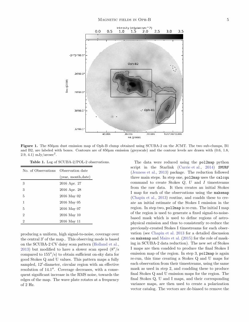
Figure 1. The 850µm dust emission map of Oph-B clump obtained using SCUBA-2 on the JCMT. The two sub-clumps, B1and B2, are labeled with boxes. Contours are of 850µm emission (greyscale) and the contour levels are drawn with (0.6, 1.8,2.9, 4.1) mJy/arcsec2 .

Table 1. Log of SCUBA-2/POL-2 observations.

No. of Observations Observation date

(year, month,date)

3 2016 Apr. 27

3 2016 Apr. 28

5 2016 May 02

1 2016 May 05

5 2016 May 07

2 2016 May 10

2 2016 May 11

producing a uniform, high signal-to-noise, coverage over

the central 3′ of the map.. This observing mode is based

on the SCUBA-2 CV daisy scan pattern (Holland et al.,

2013) but modified to have a slower scan speed (8′′/s

compared to 155′′/s) to obtain sufficient on-sky data forgood Stokes Q and U values. This pattern maps a fully

sampled, 12′-diameter, circular region with an effective

resolution of 14.1′′. Coverage decreases, with a conse-

quent significant increase in the RMS noise, towards theedges of the map. The wave plate rotates at a frequency

of 2 Hz.

The data were reduced using the pol2map python

script in the Starlink (Currie et al., 2014) SMURF

(Jenness et al., 2013) package. The reduction followed

three main steps. In step one, pol2map uses the calcqu

command to create Stokes Q, U and I timestreams

from the raw data. It then creates an initial Stokes

I map for each of the observations using the makemap

(Chapin et al., 2013) routine, and coadds these to cre-

ate an initial estimate of the Stokes I emission in the

region. In step two, pol2map is re-run. The initial I map

of the region is used to generate a fixed signal-to-noise-based mask which is used to define regions of astro-

physical emission and thus to consistently re-reduce the

previously-created Stokes I timestreams for each obser-

vation (see Chapin et al. 2013 for a detailed discussion

on makemap and Mairs et al. (2015) for the role of mask-ing in SCUBA-2 data reduction). The new set of Stokes

I maps are then coadded to produce the final Stokes I

emission map of the region. In step 3, pol2map is again

re-run, this time creating a Stokes Q and U maps foreach observation from their timestreams, using the same

mask as used in step 2, and coadding these to produce

final Stokes Q and U emission maps for the region. The

final Stokes Q, U and I maps, and their corresponding

variance maps, are then used to create a polarizationvector catalog. The vectors are de-biased to remove the

6 Soam et al.

effect of statistical biasing in low signal-to-noise-ratio

(SNR) regions. See Mairs et al. (2015) and Pattle et al.

(2017) for a detailed description of the SCUBA-2 and

POL-2 data reduction process, respectively.The RMS noise in the maps was estimated by selecting

an emission-free region near the map center and find-

ing the standard deviation of the measured flux den-

sity distribution in that region. A RMS noise value of

∼2 mJy/beam (Pattle et al., 2017) was set as the targetvalue for the BISTRO survey. The estimated noise in

the Stokes I map of Oph-B is ∼ 3.5 mJy/beam.

Bias in the measured polarization fraction and po-

larized intensity values result from the fact that polar-ized intensity is defined as being positive, and so un-

certainties on Stokes Q and U values tend to increase

the measured polarization values (Vaillancourt, 2006;

Kwon et al., 2018). De-biased values of polarized in-

tensity are estimated to be

PI =√

Q2 +U2 − 0.5(δQ2 + δU2), (1)

where PI is polarized intensity, δQ is the uncertainty

on Stokes Q, and δU is the uncertainty on Stokes U. The

polarization fraction, P, is then given by

P =PI

I, (2)

where I is the total intensity.The polarization position angle θ and the correspond-

ing uncertainties (Naghizadeh-Khouei & Clarke, 1993)

are estimated as:

θ =1

2tan−1(

U

Q), (3)

and

δθ = 0.5×√

(Q2 × δU2 +U2 × δQ2)

(Q2 +U2)×

180◦

π(4)

The debiased polarized intensity, polarization fractionand angle derived as explained above are used in the

analysis of the paper. Magnetic field orientation is de-

rived by rotating the θ by 90◦. The details of the pro-

cedure followed in producing polarization values is ex-plained in detail by Kwon et al. (2018).

3. RESULTS

Figure 1 shows the Stokes I map of Oph-B obtained

from SCUBA-2/POL-2 observations. The Oph-B clumpcontains two structures, one in the southwest known as

Oph-B1 and other in the northeast known as Oph-B2

(Motte et al., 1998). These structures are labeled with

boxes in figure 1. The entire clump appears to be rather

cold, with dust temperatures ranging from ∼ 7 to 23 K

at the center of the clump (Stamatellos et al., 2007).

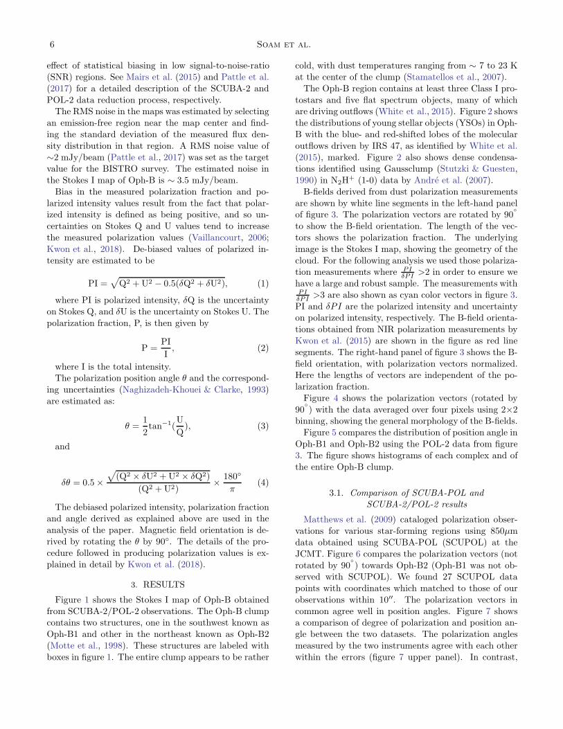
The Oph-B region contains at least three Class I pro-

tostars and five flat spectrum objects, many of whichare driving outflows (White et al., 2015). Figure 2 shows

the distributions of young stellar objects (YSOs) in Oph-

B with the blue- and red-shifted lobes of the molecular

outflows driven by IRS 47, as identified by White et al.

(2015), marked. Figure 2 also shows dense condensa-tions identified using Gaussclump (Stutzki & Guesten,

1990) in N2H+ (1-0) data by Andre et al. (2007).

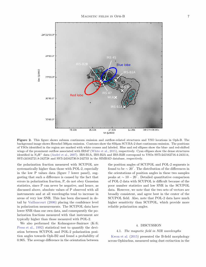
B-fields derived from dust polarization measurements

are shown by white line segments in the left-hand panelof figure 3. The polarization vectors are rotated by 90

◦

to show the B-field orientation. The length of the vec-

tors shows the polarization fraction. The underlying

image is the Stokes I map, showing the geometry of the

cloud. For the following analysis we used those polariza-tion measurements where PI

δPI>2 in order to ensure we

have a large and robust sample. The measurements withPIδPI

>3 are also shown as cyan color vectors in figure 3.

PI and δPI are the polarized intensity and uncertaintyon polarized intensity, respectively. The B-field orienta-

tions obtained from NIR polarization measurements by

Kwon et al. (2015) are shown in the figure as red line

segments. The right-hand panel of figure 3 shows the B-

field orientation, with polarization vectors normalized.Here the lengths of vectors are independent of the po-

larization fraction.

Figure 4 shows the polarization vectors (rotated by

90◦

) with the data averaged over four pixels using 2×2binning, showing the general morphology of the B-fields.

Figure 5 compares the distribution of position angle in

Oph-B1 and Oph-B2 using the POL-2 data from figure

3. The figure shows histograms of each complex and of

the entire Oph-B clump.

3.1. Comparison of SCUBA-POL andSCUBA-2/POL-2 results

Matthews et al. (2009) cataloged polarization obser-

vations for various star-forming regions using 850µm

data obtained using SCUBA-POL (SCUPOL) at the

JCMT. Figure 6 compares the polarization vectors (not

rotated by 90◦

) towards Oph-B2 (Oph-B1 was not ob-served with SCUPOL). We found 27 SCUPOL data

points with coordinates which matched to those of our

observations within 10′′. The polarization vectors in

common agree well in position angles. Figure 7 showsa comparison of degree of polarization and position an-

gle between the two datasets. The polarization angles

measured by the two instruments agree with each other

within the errors (figure 7 upper panel). In contrast,

Magnetic fields in Oph-B 7

Figure 2. This figure shows submm continuum emission and outflow-related structures and YSO locations in Oph-B. Thebackground image shows Herschel 500µm emission. Contours show the 850µm SCUBA-2 dust continuum emission. The positionsof YSOs identified in the region are marked with white crosses and labeled. Blue and red ellipses show the blue- and red-shiftedwings of the prominent outflow associated with IRS47 (White et al., 2015), respectively. Cyan ellipses show the dense structuresidentified in N2H+ data (Andre et al., 2007). IRS-B1A, IRS-B2A and IRS-B2B correspond to YSOs SSTc2dJ162716.4-243114,SSTc2d162721.8-242728 and SSTc2d162730.9-242733 in the SIMBAD database, respectively.

the polarization fraction measured with SCUPOL are

systematically higher than those with POL-2, especially

in the low P values data (figure 7 lower panel), sug-gesting that such a difference is caused by the fact that

errors in polarization fraction, P, do not obey Gaussian

statistics, since P can never be negative, and hence, as

discussed above, absolute values of P observed with all

instruments and at all wavelengths tend to increase inareas of very low SNR. This has been discussed in de-

tail by Vaillancourt (2006) placing the confidence level

in polarization measurements. The SCUPOL data have

lower SNR than our own data, and consequently the po-larization fractions measured with that instrument are

typically higher than those measured with POL-2.

We also performed the Kolmogorov-Smirnov (K-S;

Press et al., 1992) statistical test to quantify the devi-

ation between SCUPOL and POL-2 polarization posi-tion angles towards Oph-B2 and found a probability of

0.905. The average difference in the orientation between

the position angles of SCUPOL and POL-2 segments is

found to be ∼ 20◦

. The distribution of the differences in

the orientations of position angles in these two samplespeaks at ∼ 10− 20

◦

. Detailed quantitative comparison

of POL-2 data with SCUPOL is difficult because of the

poor number statistics and low SNR in the SCUPOL

data. However, we note that the two sets of vectors are

broadly consistent, and agree best in the center of theSCUPOL field. Also, note that POL-2 data have much

higher sensitivity than SCUPOL, which provide more

reliable polarization angles.

4. DISCUSSION

4.1. The magnetic field in NIR wavelengths

Kwon et al. (2015) presented the B-field morphology

across Ophiuchus, measured using dust extinction in the

8 Soam et al.

Figure 3. Left panel: B-field orientation in Oph-B from 850µm dust polarization data. The background image shows the dustcontinuum map at 850µm from SCUBA-2. The white and cyan color vectors correspond to data with PI/δPI > 2 and PI/δPI >

3, respectively. The vectors are rotated by 90◦

to show the inferred B-field morphology. The white star symbol represents theposition of IRS47, with its associated bipolar outflow shown using a double-headed arrow in yellow. A 5% polarization vector isshown for reference. The red vectors shows the B-fields mapped using deep NIR observations by (Kwon et al., 2015). The blackdashed line shows the orientation of the Galactic Plane at the latitude of the cloud. Right panel: Same as left panel (exceptNIR data), but the vectors are of uniform length, rather than scaled with polarization fraction.

J, H and K bands using SIRPOL1. Near-infrared (NIR)

polarimetry can probe B-fields in diffuse environments(AV ∼ 10− 20 mag; Tamura 1999; Tamura et al. 2011).

However, these data cannot probe the high-density re-

gions where stars themselves form. To study the B-

field morphology on .1 pc scales, Kwon et al. (2015)compared the NIR data with optical polarimetry data

tracing B-fields on 1-10 pc scales in the Ophiuchus re-

gion (Vrba et al., 1976). Their investigation suggested

that the B-field structures in the Ophiuchus clumps were

distorted by the cluster formation in this region, whichmay have been induced by a shock compression by winds

and/or radiation from the Scorpius−Centaurus associ-

ation towards its west. The overall B-field observed at

NIR wavelengths is found to have an orientation of 50◦

East of North (Kwon et al., 2015).

4.2. The magnetic field morphology in submm

wavelengths

Submm polarimetry probes B-fields in relatively dense

(AV ∼ 50 mag) regions of clouds. It can be noticed in

1 SIRIUS camera in POLarimeter mode on the IRSF 1.4 mtelescope in South Africa (Kandori et al., 2006)

figure 5 that the distribution of position angles peaks

at θ= 50-80◦

, suggesting that the large-scale B-field isa dominant component of the cloud’s B-field geometry.

There is a more clearly prevailing B-field orientation in

Oph-B2, as demonstrated by the peak in the distribu-

tion shown in the histogram. The 1000-2000 AU-scaleB-field traced by 850µm polarimetry seems to follow the

structure of the two clumps, if we consider the field ge-

ometry as a whole. In figure 3, it is clear that a B-field

component with an orientation of 50-80◦

is present in

the low-density periphery of the cloud, and seems to beconnecting well to the large-scale B-fields revealed at

NIR wavelengths (shown as red vectors in the figure).

This component is also present in Planck polarization

observations (Planck Collaboration et al., 2015). Thisorientation is also supported by the position angle of a

single isolated detection in the south-east of the Oph-

B region, which has a position angle ∼60◦

. The mean

magnetic field direction in Oph-B2 by Gaussian fitting

to the position angles is measured to be 78±40◦

. Theposition angle of Oph-B2 major axis is found to be 60

◦

inferred by fitting an ellipse to the clump. The angu-

lar offset between the mean B-field direction and the

major axis of Oph-B2 suggests that the B-field is con-

Magnetic fields in Oph-B 9

16h27m10.00s20.00s30.00s40.00sRA (J2000)

32'00.0"

30'00.0"

28'00.0"

26'00.0"

-24°24'00.0"

Dec

(J2000)

5% POL-2

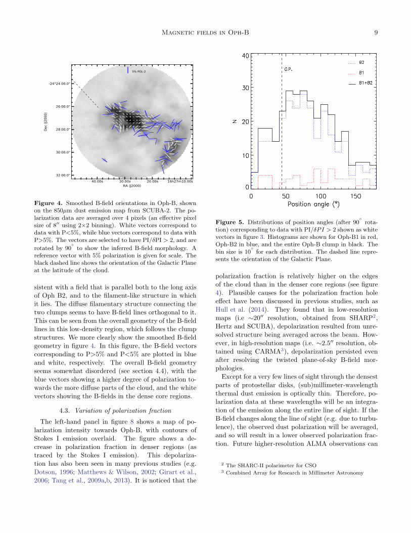
Figure 4. Smoothed B-field orientations in Oph-B, shownon the 850µm dust emission map from SCUBA-2. The po-larization data are averaged over 4 pixels (an effective pixelsize of 8′′ using 2×2 binning). White vectors correspond todata with P<5%, while blue vectors correspond to data withP>5%. The vectors are selected to have PI/δPI > 2, and are

rotated by 90◦

to show the inferred B-field morphology. Areference vector with 5% polarization is given for scale. Theblack dashed line shows the orientation of the Galactic Planeat the latitude of the cloud.

sistent with a field that is parallel both to the long axisof Oph B2, and to the filament-like structure in which

it lies. The diffuse filamentary structure connecting the

two clumps seems to have B-field lines orthogonal to it.

This can be seen from the overall geometry of the B-fieldlines in this low-density region, which follows the clump

structures. We more clearly show the smoothed B-field

geometry in figure 4. In this figure, the B-field vectors

corresponding to P>5% and P<5% are plotted in blue

and white, respectively. The overall B-field geometryseems somewhat disordered (see section 4.4), with the

blue vectors showing a higher degree of polarization to-

wards the more diffuse parts of the cloud, and the white

vectors showing the B-fields in the dense core regions.

4.3. Variation of polarization fraction

The left-hand panel in figure 8 shows a map of po-

larization intensity towards Oph-B, with contours of

Stokes I emission overlaid. The figure shows a de-

crease in polarization fraction in denser regions (astraced by the Stokes I emission). This depolariza-

tion has also been seen in many previous studies (e.g.

Dotson, 1996; Matthews & Wilson, 2002; Girart et al.,

2006; Tang et al., 2009a,b, 2013). It is noticed that the

Figure 5. Distributions of position angles (after 90◦

rota-tion) corresponding to data with PI/δPI > 2 shown as whitevectors in figure 3. Histograms are shown for Oph-B1 in red,Oph-B2 in blue, and the entire Oph-B clump in black. Thebin size is 10

◦

for each distribution. The dashed line repre-sents the orientation of the Galactic Plane.

polarization fraction is relatively higher on the edgesof the cloud than in the denser core regions (see figure

4). Plausible causes for the polarization fraction hole

effect have been discussed in previous studies, such as

Hull et al. (2014). They found that in low-resolution

maps (i.e ∼20′′ resolution, obtained from SHARP2,Hertz and SCUBA), depolarization resulted from unre-

solved structure being averaged across the beam. How-

ever, in high-resolution maps (i.e. ∼2.5′′ resolution, ob-

tained using CARMA3), depolarization persisted evenafter resolving the twisted plane-of-sky B-field mor-

phologies.

Except for a very few lines of sight through the densest

parts of protostellar disks, (sub)millimeter-wavelength

thermal dust emission is optically thin. Therefore, po-larization data at these wavelengths will be an integra-

tion of the emission along the entire line of sight. If the

B-field changes along the line of sight (e.g. due to turbu-

lence), the observed dust polarization will be averaged,and so will result in a lower observed polarization frac-

tion. Future higher-resolution ALMA observations can

2 The SHARC-II polarimeter for CSO3 Combined Array for Research in Millimeter Astronomy

10 Soam et al.

16h27m10.00s20.00s30.00s40.00s50.00sRA (J2000)

32'00.0"

30'00.0"

28'00.0"

26'00.0"

24'00.0"

-24°22'00.0"

Dec (J2000)

5% SCUPOL

16h27m10.00s20.00s30.00s40.00sRA (J2000)

32'00.0"

30'00.0"

28'00.0"

26'00.0"

-24°24'00.0"

Dec (J2000)

5% POL-2

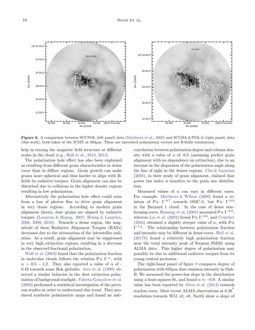
Figure 6. A comparison between SCUPOL (left panel) data (Matthews et al., 2009) and SCUBA-2/POL-2 (right panel) data(this work), both taken at the JCMT at 850µm. These are unrotated polarization vectors not B-fields orientations.

help in tracing the magnetic field structure at different

scales in the cloud (e.g., Hull et al., 2013, 2014).

The polarization hole effect has also been explained

as resulting from different grain characteristics in densecores than in diffuse regions. Grain growth can make

grains more spherical and thus harder to align with B-

fields by radiative torques. Grain alignment can also be

disturbed due to collisions in the higher density regions

resulting in low polarization.Alternatively the polarization hole effect could arise

from a loss of photon flux to drive grain alignment

in very dense regions. According to modern grain

alignment theory, dust grains are aligned by radiativetorques (Lazarian & Hoang, 2007; Hoang & Lazarian,

2008, 2009, 2016). Towards a dense region, the mag-

nitude of these Radiative Alignment Torques (RATs)

decreases due to the attenuation of the interstellar radi-

ation. As a result, grain alignment may be suppressedin very high extinction regions, resulting in a decrease

in the observed fractional polarization.

Wolf et al. (2003) found that the polarization fraction

in molecular clouds follows the relation P∝ I−α, withα ∼ 0.5 − 1.2. They also reported a value of α of -

0.43 towards some Bok globules. Arce et al. (1998) ob-

served a similar behavior in the dust extinction polar-

ization of background starlight. Falceta-Goncalves et al.

(2008) performed a statistical investigation of the previ-ous studies in order to understand this trend. They pro-

duced synthetic polarimetric maps and found an anti-

correlation between polarization degree and column den-

sity with a value of α of -0.5 (assuming perfect grain

alignment with no dependence on extinction), due to an

increase in the dispersion of the polarization angle alongthe line of sight in the denser regions. Cho & Lazarian

(2005), in their study of grain alignment, claimed that

power law index is sensitive to the grain size distribu-

tion.

Measured values of α can vary in different cases.For example, Matthews & Wilson (2000) found a re-

lation of P∝ I−0.7 towards OMC-3, but P∝ I−0.8

in the Barnard 1 cloud. In the case of dense star-

forming cores, Henning et al. (2001) measured P∝ I−0.6,whereas Lai et al. (2002) found P∝ I−0.8, and Crutcher

(2004) obtained a slightly steeper value of α, with P∝I−1.2. The relationship between polarization fraction

and intensity may be different in dense cores. Hull et al.

(2017b) found a relatively high polarization fractionnear the total intensity peak of Serpens SMM1 using

ALMA data. This higher degree of polarization may

possibly be due to additional radiative torques from its

young central protostar.The right-hand panel of figure 8 compares degree of

polarization with 850µm dust emission intensity in Oph-

B. We measured the power-law slope in the distribution

using a least-squares fit, and found α ≈ −0.9. A similar

value has been reported by Alves et al. (2014) towards

starless cores. Most recent ALMA observations at 0.26′′

resolution towards W51 e2, e8, North show a slope of

Magnetic fields in Oph-B 11

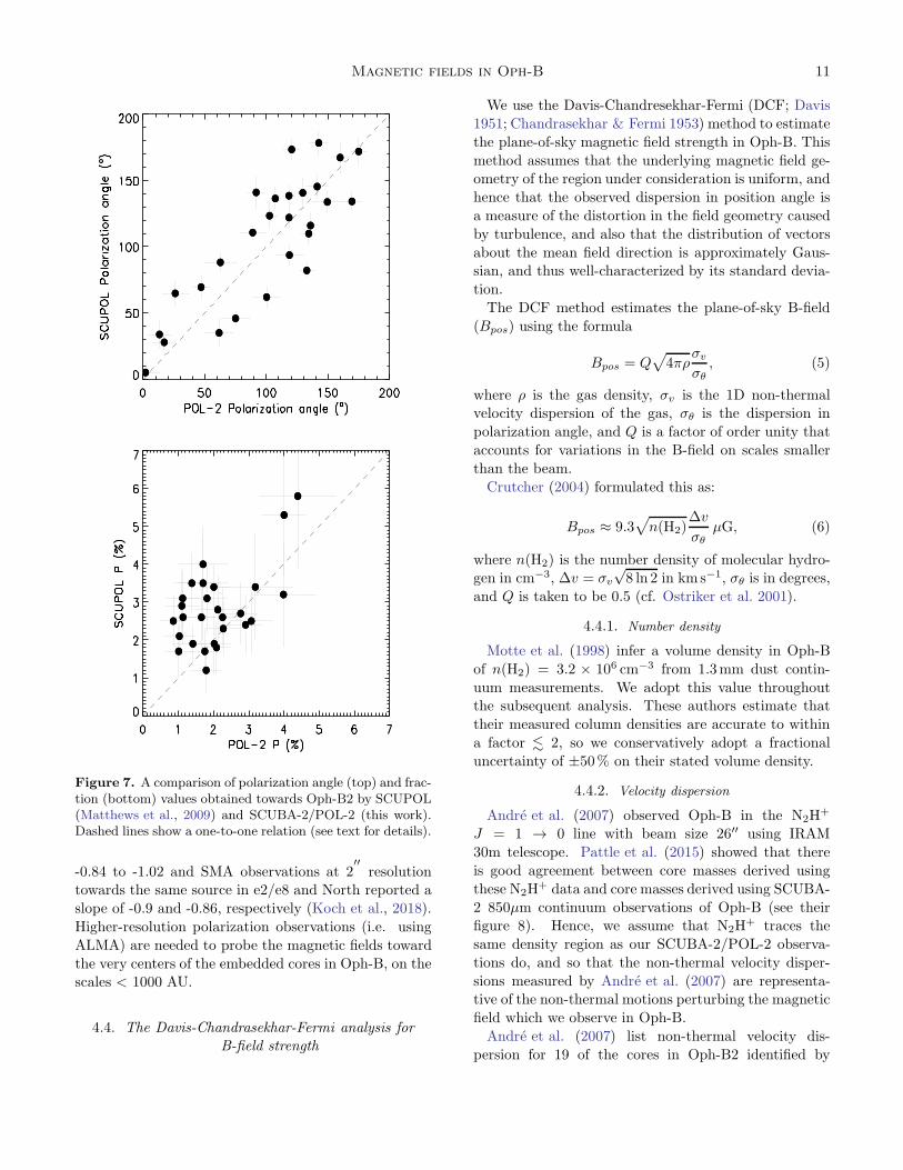
Figure 7. A comparison of polarization angle (top) and frac-tion (bottom) values obtained towards Oph-B2 by SCUPOL(Matthews et al., 2009) and SCUBA-2/POL-2 (this work).Dashed lines show a one-to-one relation (see text for details).

-0.84 to -1.02 and SMA observations at 2′′

resolutiontowards the same source in e2/e8 and North reported a

slope of -0.9 and -0.86, respectively (Koch et al., 2018).

Higher-resolution polarization observations (i.e. using

ALMA) are needed to probe the magnetic fields toward

the very centers of the embedded cores in Oph-B, on thescales < 1000 AU.

4.4. The Davis-Chandrasekhar-Fermi analysis forB-field strength

We use the Davis-Chandresekhar-Fermi (DCF; Davis

1951; Chandrasekhar & Fermi 1953) method to estimate

the plane-of-sky magnetic field strength in Oph-B. This

method assumes that the underlying magnetic field ge-ometry of the region under consideration is uniform, and

hence that the observed dispersion in position angle is

a measure of the distortion in the field geometry caused

by turbulence, and also that the distribution of vectors

about the mean field direction is approximately Gaus-sian, and thus well-characterized by its standard devia-

tion.

The DCF method estimates the plane-of-sky B-field

(Bpos) using the formula

Bpos = Q√

4πρσv

σθ

, (5)

where ρ is the gas density, σv is the 1D non-thermalvelocity dispersion of the gas, σθ is the dispersion in

polarization angle, and Q is a factor of order unity that

accounts for variations in the B-field on scales smaller

than the beam.

Crutcher (2004) formulated this as:

Bpos ≈ 9.3√

n(H2)∆v

σθ

µG, (6)

where n(H2) is the number density of molecular hydro-gen in cm−3, ∆v = σv

√8 ln 2 in kms−1, σθ is in degrees,

and Q is taken to be 0.5 (cf. Ostriker et al. 2001).

4.4.1. Number density

Motte et al. (1998) infer a volume density in Oph-B

of n(H2) = 3.2 × 106 cm−3 from 1.3mm dust contin-

uum measurements. We adopt this value throughoutthe subsequent analysis. These authors estimate that

their measured column densities are accurate to within

a factor . 2, so we conservatively adopt a fractional

uncertainty of ±50% on their stated volume density.

4.4.2. Velocity dispersion

Andre et al. (2007) observed Oph-B in the N2H+

J = 1 → 0 line with beam size 26′′ using IRAM

30m telescope. Pattle et al. (2015) showed that there

is good agreement between core masses derived using

these N2H+ data and core masses derived using SCUBA-

2 850µm continuum observations of Oph-B (see theirfigure 8). Hence, we assume that N2H

+ traces the

same density region as our SCUBA-2/POL-2 observa-

tions do, and so that the non-thermal velocity disper-

sions measured by Andre et al. (2007) are representa-tive of the non-thermal motions perturbing the magnetic

field which we observe in Oph-B.

Andre et al. (2007) list non-thermal velocity dis-

persion for 19 of the cores in Oph-B2 identified by

12 Soam et al.

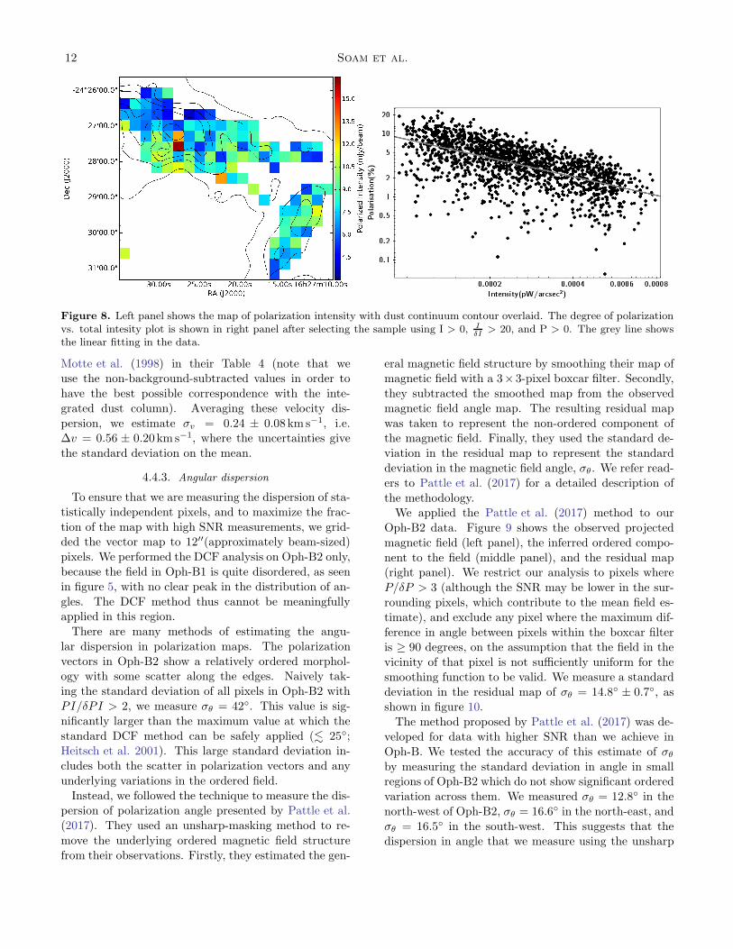
Figure 8. Left panel shows the map of polarization intensity with dust continuum contour overlaid. The degree of polarizationvs. total intesity plot is shown in right panel after selecting the sample using I > 0, I

δI> 20, and P > 0. The grey line shows

the linear fitting in the data.

Motte et al. (1998) in their Table 4 (note that weuse the non-background-subtracted values in order to

have the best possible correspondence with the inte-

grated dust column). Averaging these velocity dis-

persion, we estimate σv = 0.24 ± 0.08km s−1, i.e.∆v = 0.56 ± 0.20km s−1, where the uncertainties give

the standard deviation on the mean.

4.4.3. Angular dispersion

To ensure that we are measuring the dispersion of sta-

tistically independent pixels, and to maximize the frac-

tion of the map with high SNR measurements, we grid-ded the vector map to 12′′(approximately beam-sized)

pixels. We performed the DCF analysis on Oph-B2 only,

because the field in Oph-B1 is quite disordered, as seen

in figure 5, with no clear peak in the distribution of an-

gles. The DCF method thus cannot be meaningfullyapplied in this region.

There are many methods of estimating the angu-

lar dispersion in polarization maps. The polarization

vectors in Oph-B2 show a relatively ordered morphol-ogy with some scatter along the edges. Naively tak-

ing the standard deviation of all pixels in Oph-B2 with

PI/δPI > 2, we measure σθ = 42◦. This value is sig-

nificantly larger than the maximum value at which the

standard DCF method can be safely applied (. 25◦;Heitsch et al. 2001). This large standard deviation in-

cludes both the scatter in polarization vectors and any

underlying variations in the ordered field.

Instead, we followed the technique to measure the dis-persion of polarization angle presented by Pattle et al.

(2017). They used an unsharp-masking method to re-

move the underlying ordered magnetic field structure

from their observations. Firstly, they estimated the gen-

eral magnetic field structure by smoothing their map ofmagnetic field with a 3× 3-pixel boxcar filter. Secondly,

they subtracted the smoothed map from the observed

magnetic field angle map. The resulting residual map

was taken to represent the non-ordered component ofthe magnetic field. Finally, they used the standard de-

viation in the residual map to represent the standard

deviation in the magnetic field angle, σθ. We refer read-

ers to Pattle et al. (2017) for a detailed description of

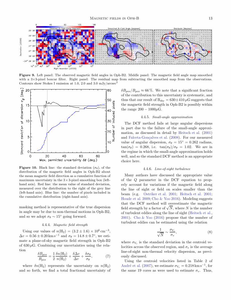
the methodology.We applied the Pattle et al. (2017) method to our

Oph-B2 data. Figure 9 shows the observed projected

magnetic field (left panel), the inferred ordered compo-

nent to the field (middle panel), and the residual map(right panel). We restrict our analysis to pixels where

P/δP > 3 (although the SNR may be lower in the sur-

rounding pixels, which contribute to the mean field es-

timate), and exclude any pixel where the maximum dif-

ference in angle between pixels within the boxcar filteris ≥ 90 degrees, on the assumption that the field in the

vicinity of that pixel is not sufficiently uniform for the

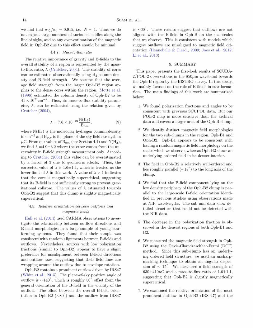
smoothing function to be valid. We measure a standard

deviation in the residual map of σθ = 14.8◦ ± 0.7◦, asshown in figure 10.

The method proposed by Pattle et al. (2017) was de-

veloped for data with higher SNR than we achieve in

Oph-B. We tested the accuracy of this estimate of σθ

by measuring the standard deviation in angle in smallregions of Oph-B2 which do not show significant ordered

variation across them. We measured σθ = 12.8◦ in the

north-west of Oph-B2, σθ = 16.6◦ in the north-east, and

σθ = 16.5◦ in the south-west. This suggests that thedispersion in angle that we measure using the unsharp

Magnetic fields in Oph-B 13

Figure 9. Left panel: The observed magnetic field angles in Oph-B2. Middle panel: The magnetic field angle map smoothedwith a 3×3-pixel boxcar filter. Right panel: The residual map from subtracting the smoothed map from the observations.Contours show Stokes I emission at 1.0, 2.0 and 3.0 mJy/arcsec2

Figure 10. Black line: the standard deviation (σθ), of thedistribution of the magnetic field angles in Oph-B2 aboutthe mean magnetic field direction as a cumulative function ofmaximum uncertainty in the 3×3-pixel smoothing box (left-hand axis). Red line: the mean value of standard deviation,measured over the distribution to the right of the grey line(left-hand axis). Blue line: the number of pixels included inthe cumulative distribution (right-hand axis).

masking method is representative of the true dispersionin angle may be due to non-thermal motions in Oph-B2,

and so we adopt σθ ∼ 15◦ going forward.

4.4.4. Magnetic field strength

Using our values of n(H2) = (3.2 ± 1.6) × 106 cm−3,

∆v = 0.56± 0.20km s−1 and σθ = 14.8± 0.7◦, we esti-

mate a plane-of-sky magnetic field strength in Oph-B2

of 630µG. Combining our uncertainties using the rela-tion

δBpos

Bpos

=1

2

δn(H2)

n(H2)+

δ∆v

∆v+

δσθ

σθ

, (7)

where δn(H2) represents the uncertainty on n(H2)

and so forth, we find a total fractional uncertainty of

δBpos/Bpos ≈ 66%. We note that a significant fraction

of the contribution to this uncertainty is systematic, andthus that our result of Bsky = 630±410µG suggests that

the magnetic field strength in Oph-B2 is possibly within

the range 200− 1000µG.

4.4.5. Small-angle approximation

The DCF method fails at large angular dispersionsin part due to the failure of the small-angle approxi-

mation, as discussed in detail by Heitsch et al. (2001)

and Falceta-Goncalves et al. (2008). For our measured

value of angular dispersion, σθ = 15◦ = 0.262 radians,tan(σθ) = 0.268, i.e. tan(σθ)/σθ = 1.02. We are in

the regime in which the small-angle approximation holds

well, and so the standard DCF method is an appropriate

choice here.

4.4.6. Line-of-sight turbulence

Many authors have discussed the appropriate value

of the Q parameter in the DCF equation to prop-

erly account for variations if the magnetic field along

the line of sight or field on scales smaller than the

beam (e.g. Ostriker et al. 2001; Heitsch et al. 2001;Houde et al. 2009; Cho & Yoo 2016). Modeling suggests

that the DCF method will overestimate the magnetic

field strength by a factor of√N , where N is the number

of turbulent eddies along the line of sight (Heitsch et al.,2001). Cho & Yoo (2016) propose that the number of

turbulent eddies can be estimated using the relation

1√N

∼σVc

σv

, (8)

where σVcis the standard deviation in the centroid ve-

locities across the observed region, and σv is the average

line-of-sight non-thermal velocity dispersion, as previ-ously discussed.

Using the centroid velocities listed in Table 2 of

Andre et al. (2007), we estimate σVc= 0.218km s−1, for

the same 19 cores as were used to estimate σv. Thus,

14 Soam et al.

we find that σVc/σv = 0.915, i.e. N ∼ 1. Thus we do

not expect large numbers of turbulent eddies along the

line of sight, and so any over-estimation of the magnetic

field in Oph-B2 due to this effect should be minimal.

4.4.7. Mass-to-flux ratio

The relative importance of gravity and B-fields to the

overall stability of a region is represented by the mass-to-flux ratio, λ (Crutcher, 2004). The stability of cores

can be estimated observationally using H2 column den-

sity and B-field strength. We assume that the aver-

age field strength from the larger Oph-B2 region ap-

plies to the dense cores within the region. Motte et al.(1998) estimated the column density of Oph-B2 to be

41× 1022cm−2. Thus, its mass-to-flux stability param-

eter, λ, can be estimated using the relation given by

Crutcher (2004),

λ = 7.6× 10−21N(H2)

Bpos

, (9)

where N(H2) is the molecular hydrogen column density

in cm−2 and Bpos is the plane-of-the sky field strength in

µG. From our values of Bpos (see Section 4.4) and N(H2),we find λ =4.9±3.2 where the error comes from the un-

certainty in B-field strength measurement only. Accord-

ing to Crutcher (2004) this value can be overestimated

by a factor of 3 due to geometric effects. Thus, the

corrected value of λ is 1.6±1.1, which is treated as thelower limit of λ in this work. A value of λ > 1 indicates

that the core is magnetically supercritical, suggesting

that its B-field is not sufficiently strong to prevent grav-

itational collapse. The values of λ estimated towardsOph-B2 suggest that this clump is slightly magnetically

supercritical.

4.5. Relative orientation between outflows and

magnetic fields

Hull et al. (2014) used CARMA observations to inves-

tigate the relationship between outflow directions and

B-field morphologies in a large sample of young star-forming systems. They found that their sample was

consistent with random alignments between B-fields and

outflows. Nevertheless, sources with low polarization

fractions (similar to Oph-B2) appear to have a slight

preference for misalignment between B-field directionsand outflow axes, suggesting that their field lines are

wrapping around the outflow due to envelope rotation.

Oph-B2 contains a prominent outflow driven by IRS47

(White et al., 2015). The plane-of-sky position angle ofoutflow is ∼140

◦

, which is roughly 50◦

offset from the

general orientation of the B-field in the vicinity of the

outflow. The offset between the overall B-field orien-

tation in Oph-B2 (∼80◦

) and the outflow from IRS47

is ∼60◦

. These results suggest that outflows are not

aligned with the B-field in Oph-B on the size scales

that we observe. This is consistent with models which

suggest outflows are misaligned to magnetic field ori-entation (Hennebelle & Ciardi, 2009; Joos et al., 2012;

Li et al., 2013).

5. SUMMARY

This paper presents the first-look results of SCUBA-

2/POL-2 observations in the 850µm waveband towardsthe Oph-B region by the BISTRO survey. In this study,

we mainly focused on the role of B-fields in star forma-

tion. The main findings of this work are summarized

below:

1. We found polarization fractions and angles to be

consistent with previous SCUPOL data. But our

POL-2 map is more sensitive than the archival

data and covers a larger area of the Oph-B clump.

2. We identify distinct magnetic field morphologies

for the two sub-clumps in the region, Oph-B1 and

Oph-B2. Oph-B1 appears to be consistent with

having a random magnetic field morphology on thescales which we observe, whereas Oph-B2 shows an

underlying ordered field in its denser interior.

3. The field in Oph-B2 is relatively well-ordered and

lies roughly parallel (∼18◦

) to the long axis of theclump.

4. We find that the B-field component lying on the

low density periphery of the Oph-B2 clump is par-allel to the large-scale B-field orientation identi-

fied in previous studies using observations made

at NIR wavelengths. The sub-mm data show de-

tailed structure that could not be detected with

the NIR data.

5. The decrease in the polarization fraction is ob-

served in the densest regions of both Oph-B1 and

B2.

6. We measured the magnetic field strength in Oph-

B2 using the Davis-Chandrasekhar-Fermi (DCF)

method. Since this sub-clump has an underly-

ing ordered field structure, we used an unsharp-masking technique to obtain an angular disper-

sion of ∼ 15◦

. We measured a field strength of

630±410µG and a mass-to-flux ratio of 1.6±1.1,

suggesting that Oph-B2 is slightly magneticallysupercritical.

7. We examined the relative orientation of the most

prominent outflow in Oph-B2 (IRS 47) and the

Magnetic fields in Oph-B 15

local magnetic field. The two have orientations

that are offset by ∼50◦

, suggesting they are not

aligned. The angular offset between the large-scale

magnetic field in Oph-B2 and the outflow orienta-tion is ∼60

◦

, suggesting consistency with models

which predict that outflows should be misaligned

to magnetic field direction.

6. ACKNOWLEDGMENTS

Authors thank referee for a constructive report that

helped in improving the content of this paper. TheJames Clerk Maxwell Telescope is operated by the East

Asian Observatory on behalf of the National Astronomi-

cal Observatory of Japan, the Academia Sinica Institute

of Astronomy and Astrophysics, the Korea Astronomyand Space Science Institute, the National Astronomi-

cal Observatories of China and the Chinese Academy

of Sciences (Grant No. XDB09000000), with additional

funding support from the Science and Technology Facil-

ities Council of the United Kingdom and participatinguniversities in the United Kingdom and Canada. The

James Clerk Maxwell Telescope has historically been op-

erated by the Joint Astronomy Centre on behalf of the

Science and Technology Facilities Council of the UnitedKingdom, the National Research Council of Canada and

the Netherlands Organisation for Scientific Research.

Additional funds for the construction of SCUBA-2 and

POL-2 were provided by the Canada Foundation for

Innovation. The data used in this paper were takenunder project code M16AL004. AS would like to ac-

knowledge the support from KASI for postdoctoral fel-

lowship. K.P. acknowledges support from the Science

and Technology Facilities Council (STFC) under grantnumber ST/M000877/1 and the Ministry of Science and

Technology, Taiwan, under grant number 106-2119-M-

007-021-MY3, and was an International Research Fel-

low of the Japan Society for the Promotion of Science

for part of the duration of this project. CWL andMK were supported by Basic Science Research Program

through the National Research Foundation of Korea

(NRF) funded by the Ministry of Education, Science and

Technology (CWL: NRF-2016R1A2B4012593) and the

Ministry of Science, ICT & Future Planning (MK: NRF-2015R1C1A1A01052160). W.K. was supported by Ba-

sic Science Research Program through the National Re-

search Foundation of Korea (NRF-2016R1C1B2013642).

JEL is supported by the Basic Science Research Pro-gram through the National Research Foundation of Ko-

rea (grant No. NRF-2018R1A2B6003423) and the Ko-

rea Astronomy and Space Science Institute under the

R&D program supervised by the Ministry of Science,

ICT and Future Planning. D.L. is supported by NSFCNo. 11725313. S.P.L. acknowledges support from the

Ministry of Science and Technology of Taiwan with

Grant MOST 106-2119-M-007-021-MY3. K.Q. acknowl-

edges the support from National Natural Science Foun-dation of China (NSFC) through grants NSFC 11473011

and NSFC 11590781. This research has made use of

the NASA Astrophysics Data System. AS thanks Ma-

heswar G. for discussion on polarization in star-forming

regions. AS also thanks Piyush Bhardwaj (GIST, SouthKorea) for a critical reading of the paper. The authors

wish to recognize and acknowledge the very significant

cultural role that the summit of Maunakea has always

had within the indigenous Hawaiian community, withreverence. AS specially thanks the JCMT TSS for the

hard-earned data.

REFERENCES

Allen, A., Li, Z.-Y., & Shu, F. H. 2003, ApJ, 599, 363

Alves, F. O., Frau, P., Girart, J. M., et al. 2014, A&A, 569,

L1

Andersson, B.-G., Lazarian, A., & Vaillancourt, J. E. 2015,

ARA&A, 53, 501

Andre, P., Belloche, A., Motte, F., & Peretto, N. 2007,

A&A, 472, 519

Arce, H. G., Goodman, A. A., Bastien, P., Manset, N., &

Sumner, M. 1998, ApJL, 499, L93

Attard, M., Houde, M., Novak, G., et al. 2009, ApJ, 702,

1584

Chandrasekhar, S., & Fermi, E. 1953, ApJ, 118, 113

Chapin, E. L., Berry, D. S., Gibb, A. G., et al. 2013,

MNRAS, 430, 2545

Chini, R. 1981, A&A, 99, 346

Cho, J., & Lazarian, A. 2005, ApJ, 631, 361

Cho, J., & Yoo, H. 2016, ApJ, 821, 21

Crutcher, R. M. 2004, Ap&SS, 292, 225

Cudlip, W., Furniss, I., King, K. J., & Jennings, R. E.

1982, MNRAS, 200, 1169

Currie, M. J., Berry, D. S., Jenness, T., et al. 2014, in

Astronomical Society of the Pacific Conference Series,

Vol. 485, Astronomical Data Analysis Software and

Systems XXIII, ed. N. Manset & P. Forshay, 391

Davis, L. 1951, Phys. Rev., 81, 890.

https://link.aps.org/doi/10.1103/PhysRev.81.890.2

de Geus, E. J., de Zeeuw, P. T., & Lub, J. 1989, A&A, 216,

44

16 Soam et al.

Dib, S., Hennebelle, P., Pineda, J. E., et al. 2010, ApJ, 723,

425

Dib, S., Kim, J., Vazquez-Semadeni, E., Burkert, A., &

Shadmehri, M. 2007, ApJ, 661, 262

Dolginov, A. Z., & Mitrofanov, I. G. 1976, Ap&SS, 43, 291

Dotson, J. L. 1996, ApJ, 470, 566

Dotson, J. L., Davidson, J., Dowell, C. D., Schleuning,

D. A., & Hildebrand, R. H. 2000, ApJS, 128, 335

Dotson, J. L., Vaillancourt, J. E., Kirby, L., et al. 2010,

ApJS, 186, 406

Falceta-Goncalves, D., Lazarian, A., & Kowal, G. 2008,

ApJ, 679, 537

Fiedler, R. A., & Mouschovias, T. C. 1993, ApJ, 415, 680

Friberg, P., Bastien, P., Berry, D., et al. 2016, in

Proc. SPIE, Vol. 9914, Millimeter, Submillimeter, and

Far-Infrared Detectors and Instrumentation for

Astronomy VIII, 991403

Galli, D., & Shu, F. H. 1993, ApJ, 417, 243

Girart, J. M., Rao, R., & Marrone, D. P. 2006, Science,

313, 812

Hall, J. S. 1949, Science, 109, 166

Heitsch, F., Zweibel, E. G., Mac Low, M.-M., Li, P., &

Norman, M. L. 2001, ApJ, 561, 800

Hennebelle, P., & Ciardi, A. 2009, A&A, 506, L29

Henning, T., Wolf, S., Launhardt, R., & Waters, R. 2001,

ApJ, 561, 871

Hildebrand, R. H. 1988, QJRAS, 29, 327

Hildebrand, R. H., Dragovan, M., & Novak, G. 1984, ApJL,

284, L51

Hiltner, W. A. 1949a, ApJ, 109, 471

—. 1949b, Science, 109, 165

Hoang, T., & Lazarian, A. 2008, MNRAS, 388, 117

—. 2009, ApJ, 697, 1316

—. 2014, MNRAS, 438, 680

—. 2016, ApJ, 831, 159

Hoang, T., Lazarian, A., & Andersson, B.-G. 2015,

MNRAS, 448, 1178

Holland, W. S., Bintley, D., Chapin, E. L., et al. 2013,

MNRAS, 430, 2513

Houde, M., Vaillancourt, J. E., Hildebrand, R. H.,

Chitsazzadeh, S., & Kirby, L. 2009, ApJ, 706, 1504

Hull, C. L. H., Plambeck, R. L., Bolatto, A. D., et al. 2013,

ApJ, 768, 159

Hull, C. L. H., Plambeck, R. L., Kwon, W., et al. 2014,

ApJS, 213, 13

Hull, C. L. H., Mocz, P., Burkhart, B., et al. 2017a, ApJL,

842, L9

Hull, C. L. H., Girart, J. M., Tychoniec, L., et al. 2017b,

ApJ, 847, 92

Jenness, T., Chapin, E. L., Berry, D. S., et al. 2013,

SMURF: SubMillimeter User Reduction Facility,

Astrophysics Source Code Library, , , ascl:1310.007

Johnstone, D., Wilson, C. D., Moriarty-Schieven, G., et al.

2000, ApJ, 545, 327

Joos, M., Hennebelle, P., & Ciardi, A. 2012, A&A, 543,

A128

Kandori, R., Kusakabe, N., Tamura, M., et al. 2006, in

Proc. SPIE, Vol. 6269, Society of Photo-Optical

Instrumentation Engineers (SPIE) Conference Series,

626951

Knude, J., & Hog, E. 1998, A&A, 338, 897

Koch, P. M., Tang, Y.-W., Ho, P. T. P., et al. 2018, ApJ,

855, 39

Kwon, J., Tamura, M., Hough, J. H., et al. 2015, ApJS,

220, 17

Kwon, J., Doi, Y., Tamura, M., et al. 2018, ArXiv e-prints,

arXiv:1804.09313

Lai, S.-P., Crutcher, R. M., Girart, J. M., & Rao, R. 2002,

ApJ, 566, 925

Lazarian, A. 2000, in Astronomical Society of the Pacific

Conference Series, Vol. 215, Cosmic Evolution and

Galaxy Formation: Structure, Interactions, and

Feedback, ed. J. Franco, L. Terlevich, O. Lopez-Cruz, &

I. Aretxaga, 69

Lazarian, A. 2007, JQSRT, 106, 225

Lazarian, A., & Hoang, T. 2007, MNRAS, 378, 910

Li, Z.-Y., Krasnopolsky, R., & Shang, H. 2013, ApJ, 774, 82

Loinard, L., Torres, R. M., Mioduszewski, A. J., &

Rodrıguez, L. F. 2008, ApJL, 675, L29

Mac Low, M.-M., & Klessen, R. S. 2004, Reviews of

Modern Physics, 76, 125

Mairs, S., Johnstone, D., Kirk, H., et al. 2015, MNRAS,

454, 2557

Matthews, B. C., McPhee, C. A., Fissel, L. M., & Curran,

R. L. 2009, ApJS, 182, 143

Matthews, B. C., & Wilson, C. D. 2000, ApJ, 531, 868

—. 2002, ApJ, 574, 822

McKee, C. F., & Ostriker, E. C. 2007, ARA&A, 45, 565

McKee, C. F., Zweibel, E. G., Goodman, A. A., & Heiles,

C. 1993, in Protostars and Planets III, ed. E. H. Levy &

J. I. Lunine, 327

Miville-Deschenes, M.-A., Martin, P. G., Abergel, A., et al.

2010, A&A, 518, L104

Motte, F., Andre, P., & Neri, R. 1998, A&A, 336, 150

Mouschovias, T. C., & Ciolek, G. E. 1999, in NATO ASIC

Proc. 540: The Origin of Stars and Planetary Systems,

ed. C. J. Lada & N. D. Kylafis, 305

Naghizadeh-Khouei, J., & Clarke, D. 1993, A&A, 274, 968

Magnetic fields in Oph-B 17

Ortiz-Leon, G. N., Loinard, L., Kounkel, M. A., et al. 2017,

ApJ, 834, 141

Ostriker, E. C., Stone, J. M., & Gammie, C. F. 2001, ApJ,

546, 980

Padgett, D. L., Rebull, L. M., Stapelfeldt, K. R., et al.

2008, ApJ, 672, 1013

Pattle, K., Ward-Thompson, D., Kirk, J. M., et al. 2015,

MNRAS, 450, 1094

Pattle, K., Ward-Thompson, D., Berry, D., et al. 2017,

ApJ, 846, 122

P.Bastien et. al. in prep. 2018, -,

Planck Collaboration, Ade, P. A. R., Aghanim, N., et al.

2015, A&A, 576, A105

Press, W. H., Rybicki, G. B., & Hewitt, J. N. 1992, ApJ,

385, 416

Rao, R., Crutcher, R. M., Plambeck, R. L., & Wright,

M. C. H. 1998, ApJL, 502, L75

Rebull, L. M., Wolff, S. C., & Strom, S. E. 2004, AJ, 127,

1029

Shu, F. H., Adams, F. C., & Lizano, S. 1987, ARA&A, 25,

23

Stamatellos, D., Whitworth, A. P., & Ward-Thompson, D.

2007, MNRAS, 379, 1390

Stutzki, J., & Guesten, R. 1990, ApJ, 356, 513

Tamura, M. 1999, in Star Formation 1999, ed.

T. Nakamoto, 212–216

Tamura, M., Hashimoto, J., Kandori, R., et al. 2011, in

Astronomical Society of the Pacific Conference Series,

Vol. 449, Astronomical Society of the Pacific Conference

Series, ed. P. Bastien, N. Manset, D. P. Clemens, &

N. St-Louis, 207

Tang, Y.-W., Ho, P. T. P., Girart, J. M., et al. 2009a, ApJ,

695, 1399

Tang, Y.-W., Ho, P. T. P., Koch, P. M., et al. 2009b, ApJ,

700, 251

Tang, Y.-W., Ho, P. T. P., Koch, P. M., Guilloteau, S., &

Dutrey, A. 2013, ApJ, 763, 135

Vaillancourt, J. E. 2006, PASP, 118, 1340

Vaillancourt, J. E., & Matthews, B. C. 2012, ApJS, 201, 13

Vrba, F. J., Strom, S. E., & Strom, K. M. 1976, AJ, 81, 958

Ward-Thompson, D., Pattle, K., Bastien, P., et al. 2017,

ApJ, 842, 66

White, G. J., Drabek-Maunder, E., Rosolowsky, E., et al.

2015, MNRAS, 447, 1996

Wilking, B. A. 1992, Star Formation in the Ophiuchus

Molecular Cloud Complex, ed. B. Reipurth, 159

Wolf, S., Launhardt, R., & Henning, T. 2003, ApJ, 592, 233