Magnetic field modeling of a dual-magnet …...Magnetic field modeling of a dual-magnet configuration Tat Joo Teo a and I-Ming Chen School of Mechanical & Aerospace Engineering,

Magnetic field modeling of a dual-magnet configurationTat Joo Teoa� and I-Ming ChenSchool of Mechanical & Aerospace Engineering, Nanyang Technological University, 50 Nanyang Avenue,Singapore 639798, Singapore

Guilin Yang and Wei LinSingapore Institute of Manufacturing Technology, Agency of Science, Technology and Research (A*STAR),71 Nanyang Drive, Singapore 638075, Singapore

�Received 2 May 2007; accepted 22 August 2007; published online 15 October 2007�

This paper presents the theoretical and experimental studies of a dual-magnet �DM� configurationthat forms the electromagnetic circuit of a nanopositioning actuator. Motivation of this work ariseswhen an accurate prediction of the magnetic field behavior within the DM configuration is requiredto achieve ultrahigh precision motion control. In the theoretical modeling, the DM configuration isdecomposed into several regions where each region is treated as a boundary-value problem. Amethod, termed superposition of the boundary conditions, is used to obtain the field solution of anair gap that is influenced by two magnetic sources. Consequently, a two-dimensional �2D� analyticalmodel that accurately predicts the magnetic field behavior of the DM configuration is presented. Inthe experimental investigations, the magnetic flux density measured from a DM configurationprototype is used to validate the accuracy of the 2D analytical model. These experimental data werealso compared against the magnetic flux density collected from a conventional single-magnetconfiguration prototype. Such comparisons verify the claimed features of the DM configuration, i.e.,providing 40% increase in the magnetic flux density and offering an evenly distributed magneticfield through the entire air gap of 11 mm. © 2007 American Institute of Physics.�DOI: 10.1063/1.2794855�

I. INTRODUCTION

Manipulation between nano- and mesoscales with largepayload and high bandwidth has always been a technologicalgap in the field of ultrahigh precision manufacturing. Tradi-tionally, most ultrahigh precision manipulators are driven us-ing piezoelectric �PZT� actuators due to their large actuatingforce and ease of control.1–7 However, PZT actuators areunsuitable for a manipulator targeted to achieve millimetersrange with resolutions in nanometers due to their limitedstrokes.8–10 Consequently, electromagnetic �EM� actuationbecomes a promising solution due to its capability of provid-ing displacements in millimeters with infinite positioningresolutions, high accelerations, and fast actuating speed. Cur-rently, EM propulsion, magnetic levitation �Maglev�, andLorentz-force actuation are the three main types of EM tech-nique for realizing ultrahigh precision manipulations. An EMpropulsion is achieved by the attraction and repulsion of aferromagnetic moving part using the EM field generatedfrom a solenoid.11–16 This technique possesses inconsistentactuating forces and eddy-current hysteresis due to the elec-tromagnetization of the ferromagnetic stators. Maglev hasbeen the most popular approach for developing supportlessand contactless multiple degree-of-freedom �DOF�manipulators.17–23 However, Maglev manipulators have un-stable behaviors and require complex control algorithms andcostly control systems.

Among these techniques, Lorentz-force actuation is a di-rect noncommutation drive, which provides a constant output

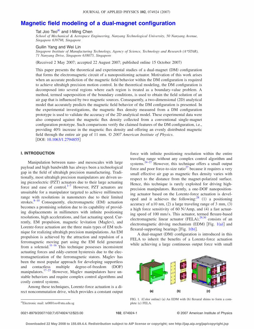
force with infinite positioning resolution within the entiretraveling range without any complex control algorithm andsystems.24–27 However, this technique offers a small outputforce and poor force-to-size ratio27 because it requires a verysmall effective air gap as magnetic flux density varies withrespect to the distance from the magnet-polarized surface.Hence, this technique is rarely exploited for driving high-precision manipulators. Recently, a one-DOF nanoposition-ing actuator based on the Lorentz-force actuation is devel-oped and it achieves the following:28 �1� a positioningaccuracy of ±10 nm, �2� a large traveling range of 3 mm, �3�a high force sensitivity of 60 N/Amp, and �4� a fast actuat-ing speed of 100 mm/s. This actuator, termed flexure-basedelectromagnetic linear actuator �FELA�,29,30 consists of anelectromagnetic driving mechanism �EDM� �Fig. 1�a�� andflexural-supporting bearings �Fig. 1�b��.

A dual-magnet �DM� configuration is introduced in thisFELA to inherit the benefits of a Lorentz-force actuationwhile achieving a large continuous output force with small

a�Electronic mail: [email protected]. 1. �Color online� �a� An EDM with �b� flexural shims to form a com-plete �c� FELA.

JOURNAL OF APPLIED PHYSICS 102, 074924 �2007�

0021-8979/2007/102�7�/074924/12/$23.00 © 2007 American Institute of Physics102, 074924-1

Downloaded 22 May 2008 to 155.69.4.4. Redistribution subject to AIP license or copyright; see http://jap.aip.org/jap/copyright.jsp

http://dx.doi.org/10.1063/1.2794855

http://dx.doi.org/10.1063/1.2794855

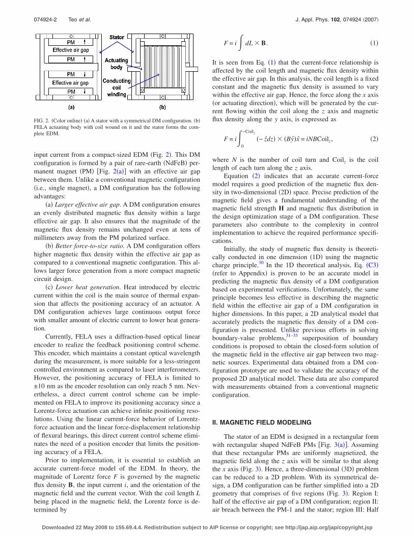
input current from a compact-sized EDM �Fig. 2�. This DMconfiguration is formed by a pair of rare-earth �NdFeB� per-manent magnet �PM� �Fig. 2�a�� with an effective air gapbetween them. Unlike a conventional magnetic configuration�i.e., single magnet�, a DM configuration has the followingadvantages:

�a� Larger effective air gap. A DM configuration ensuresan evenly distributed magnetic flux density within a largeeffective air gap. It also ensures that the magnitude of themagnetic flux density remains unchanged even at tens ofmillimeters away from the PM polarized surface.

�b� Better force-to-size ratio. A DM configuration offershigher magnetic flux density within the effective air gap ascompared to a conventional magnetic configuration. This al-lows larger force generation from a more compact magneticcircuit design.

�c� Lower heat generation. Heat introduced by electriccurrent within the coil is the main source of thermal expan-sion that affects the positioning accuracy of an actuator. ADM configuration achieves large continuous output forcewith smaller amount of electric current to lower heat genera-tion.

Currently, FELA uses a diffraction-based optical linearencoder to realize the feedback positioning control scheme.This encoder, which maintains a constant optical wavelengthduring the measurement, is more suitable for a less-stringentcontrolled environment as compared to laser interferometers.However, the positioning accuracy of FELA is limited to±10 nm as the encoder resolution can only reach 5 nm. Nev-ertheless, a direct current control scheme can be imple-mented on FELA to improve its positioning accuracy since aLorentz-force actuation can achieve infinite positioning reso-lutions. Using the linear current-force behavior of Lorentz-force actuation and the linear force-displacement relationshipof flexural bearings, this direct current control scheme elimi-nates the need of a position encoder that limits the position-ing accuracy of a FELA.

Prior to implementation, it is essential to establish anaccurate current-force model of the EDM. In theory, themagnitude of Lorentz force F is governed by the magneticflux density B, the input current i, and the orientation of themagnetic field and the current vector. With the coil length Lbeing placed in the magnetic field, the Lorentz force is de-termined by

F = i� dL � B . �1�

It is seen from Eq. �1� that the current-force relationship isaffected by the coil length and magnetic flux density withinthe effective air gap. In this analysis, the coil length is a fixedconstant and the magnetic flux density is assumed to varywithin the effective air gap. Hence, the force along the x axis�or actuating direction�, which will be generated by the cur-rent flowing within the coil along the z axis and magneticflux density along the y axis, is expressed as

F = i�0

−Coilz

�− zdz� � �By�x = iNBCoilz, �2�

where N is the number of coil turn and Coilz is the coillength of each turn along the z axis.

Equation �2� indicates that an accurate current-forcemodel requires a good prediction of the magnetic flux den-sity in two-dimensional �2D� space. Precise prediction of themagnetic field gives a fundamental understanding of themagnetic field strength H and magnetic flux distribution inthe design optimization stage of a DM configuration. Theseparameters also contribute to the complexity in controlimplementation to achieve the required performance specifi-cations.

Initially, the study of magnetic flux density is theoreti-cally conducted in one dimension �1D� using the magneticcharge principle.30 In the 1D theoretical analysis, Eq. �C3��refer to Appendix� is proven to be an accurate model inpredicting the magnetic flux density of a DM configurationbased on experimental verifications. Unfortunately, the sameprinciple becomes less effective in describing the magneticfield within the effective air gap of a DM configuration inhigher dimensions. In this paper, a 2D analytical model thataccurately predicts the magnetic flux density of a DM con-figuration is presented. Unlike previous efforts in solvingboundary-value problems,31–33 superposition of boundaryconditions is proposed to obtain the closed-form solution ofthe magnetic field in the effective air gap between two mag-netic sources. Experimental data obtained from a DM con-figuration prototype are used to validate the accuracy of theproposed 2D analytical model. These data are also comparedwith measurements obtained from a conventional magneticconfiguration.

II. MAGNETIC FIELD MODELING

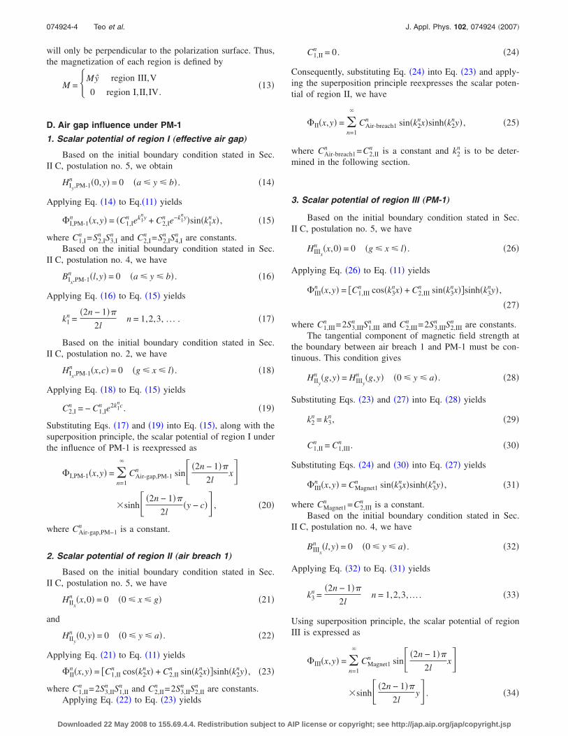
The stator of an EDM is designed in a rectangular formwith rectangular shaped NdFeB PMs �Fig. 3�a��. Assumingthat these rectangular PMs are uniformly magnetized, themagnetic field along the z axis will be similar to that alongthe x axis �Fig. 3�. Hence, a three-dimensional �3D� problemcan be reduced to a 2D problem. With its symmetrical de-sign, a DM configuration can be further simplified into a 2Dgeometry that comprises of five regions �Fig. 3�. Region I:half of the effective air gap of a DM configuration; region II:air breach between the PM-1 and the stator; region III: Half

FIG. 2. �Color online� �a� A stator with a symmetrical DM configuration. �b�FELA actuating body with coil wound on it and the stator forms the com-plete EDM.

074924-2 Teo et al. J. Appl. Phys. 102, 074924 �2007�


of the PM-1 of a DM configuration; region IV: air breachbetween the PM-2 and the stator; and region V: half of thePM-2 of a DM configuration.

A. Assumptions

In this analysis, PMs are assumed to be ideal with fieldrelationship described by the linear second quadrant of a PMdemagnetization curve. The constitutive relation for a PM isexpressed as34

B = �0�H + M� , �3�

where �0 is the permeability of the free space and M is themagnetization of a PM.

The air gap is assumed to be a linear homogeneous me-dia with the absence of magnetization, which leads to a con-stitutive relation for the air gap. This gives

B = �0H . �4�

With the assumption of a current-free air gap, the vector fieldbecomes an irrotational field and the magnetic field strengthis described by the divergence of the scalar potential �,

H = − �� . �5�

B. Boundary-value problem

The magnetic field within a current-free environment iscommonly described by Laplace’s equation, which is ex-pressed as

�2� = 0. �6�

In this analysis, the method of separation of variables is usedto obtain the solution of the scalar potential since Eq. �6� is alinear homogeneous partial differentiation equation. By let-ting the scalar potential to be a product of single variablefunction, this yields

�i�x,y� = Xi�x�Yi�y� , �7�

where i=1,2 ,3 ,4 ,5 representing region I to region V, re-spectively �Fig. 3�. Based on Eq. �7�, Eq. �6� is further ex-panded into two independent terms and yields

Xi�x�Xi�x�

+Yi��y�Yi�y�

= 0, �8�

where each term is a function of a single variable that can berepresented by an arbitrary constant, i.e., ki,x

2 +ki,y2 =0 with

Xi�x�=�2Xi�x� /�x2 and Yi��x�=�2Yi�y� /�y2.In this analysis, ki,x

2 is chosen to be a negative valuebecause with the magnetic field behavior is unpredictablealong the x axis. On the other hand, ki,y

2 is chosen to be apositive value since the magnetic field increases or decreasesaccording to the distance from the PM polarized surfacealong the y axis. Based on these conditions, Eq. �8� is sepa-rated into two independent ordinary differentiation equations�ODEs�. Solving those ODEs yield

Xin�x� = S1,i

n cos�kinx� + S2,i

n sin�kinx� �9�

and

Yin�y� = S3,i

n ekiny + S4,i

n e−kiny , �10�

where Sj,in �j=1,2 ,3 ,4� are constants.

Using Eqs. �7�, �9�, �10�, and the superposition principleyields the general form of scalar potential solution for eachregion, which is expressed as

�i�x,y� = �n=1

�

�S1,in cos�ki

nx� + S2,in sin�ki

nx��

��S3,in eki

ny + S4,in e−ki

ny� , �11�

where each constant is determined by imposing appropriateboundary conditions to each region.

C. Boundary conditions

In this analysis, superposition of boundary conditions isemployed to obtain a closed-form solution for the scalar po-tential of the effective air gap between two magnetic sources,PM-1 and PM-2. The scalar potential of the effective air gapwill be solved separately under the influence of each PM andsubsequently superimposed together. Thus, the total scalarpotential �I,Total�x ,y� of the effective air gap is expressed as

�I,Total�x,y� = �I,PM-1�x,y� + �I,PM-2�x,y� , �12�

where �I,PM-1�x ,y� is the scalar potential of effective air gapunder the influence of PM-1 and �I,PM-2�x ,y� is that underthe influence of PM-2.

Generally, initial boundary conditions are formulated un-der the following assumptions: �1� Permeability of the ironstator is infinite ��=0�. �2� When analyzing the effective airgap under the influence of PM-1, PM-2 is treated as a free-airregion. Thus, the tangential component vanishes when ap-proaching c along y axis �refer to Fig. 3�. �3� When analyz-ing the effective air gap under the influence of PM-2, PM-1is treated as a free-air region. Thus, the tangential componentvanishes when approaching 0 along y axis �refer to Fig. 3�.�4�The normal component of the magnetic flux density in themiddle of the effective air gap and the PMs is equal to zero�refer to Fig. 3 at x= l�. �5� The tangential component of themagnetic field strength along the closed-loop path is equal tozero. �6� The orientation of the magnetization within a PM

FIG. 3. �Color online� A 2D geometry reduced from half of a DMconfiguration.



will only be perpendicular to the polarization surface. Thus,the magnetization of each region is defined by

M = �My region III,V

0 region I,II,IV.� �13�

D. Air gap influence under PM-1

1. Scalar potential of region I „effective air gap…

Based on the initial boundary condition stated in Sec.II C, postulation no. 5, we obtain

HIy,PM-1n �0,y� = 0 �a � y � b� . �14�

Applying Eq. �14� to Eq.�11� yields

�I,PM-1n �x,y� = �C1,I

n ek1ny + C2,I

n e−k1ny�sin�k1

nx� , �15�

where C1,In =S2,I

n S3,In and C2,I

n =S2,In S4,I

n are constants.Based on the initial boundary condition stated in Sec.

II C, postulation no. 4, we have

BIx,PM-1n �l,y� = 0 �a � y � b� . �16�

Applying Eq. �16� to Eq. �15� yields

k1n =

�2n − 1��2l

n = 1,2,3, . . . . �17�

Based on the initial boundary condition stated in Sec.II C, postulation no. 2, we have

HIx,PM-1n �x,c� = 0 �g � x � l� . �18�


C2,In = − C1,I

n e2k1nc. �19�

Substituting Eqs. �17� and �19� into Eq. �15�, along with thesuperposition principle, the scalar potential of region I underthe influence of PM-1 is reexpressed as

�I,PM-1�x,y� = �n=1

�

CAir-gap,PM-1n sin �2n − 1��

2lx

�sinh �2n − 1��2l

�y − c� , �20�

where CAir-gap,PM−1n is a constant.

2. Scalar potential of region II „air breach 1…


HIIx

n �x,0� = 0 �0 � x � g� �21�

and

HIIy

n �0,y� = 0 �0 � y � a� . �22�


�IIn �x,y� = �C1,II

n cos�k2nx� + C2,II

n sin�k2nx��sinh�k2

ny� , �23�

where C1,IIn =2S3,II

n S1,IIn and C2,II

n =2S3,IIn S2,II

n are constants.Applying Eq. �22� to Eq. �23� yields

C1,IIn = 0. �24�

Consequently, substituting Eq. �24� into Eq. �23� and apply-ing the superposition principle reexpresses the scalar poten-tial of region II, we have

�II�x,y� = �n=1

�

CAir-breach1n sin�k2

nx�sinh�k2ny� , �25�

where CAir-breach1n =C2,II

n is a constant and k2n is to be deter-

mined in the following section.

3. Scalar potential of region III „PM-1…


HIIIx

n �x,0� = 0 �g � x � l� . �26�


�IIIn �x,y� = �C1,III

n cos�k3nx� + C2,III


ny� ,

�27�

where C1,IIIn =2S3,III

n S1,IIIn and C2,III

n =2S3,IIIn S2,III

n are constants.The tangential component of magnetic field strength at

the boundary between air breach 1 and PM-1 must be con-tinuous. This condition gives

HIIy

n �g,y� = HIIIy

n �g,y� �0 � y � a� . �28�

Substituting Eqs. �23� and �27� into Eq. �28� yields

k2n = k3

n, �29�

C1,IIn = C1,III

n . �30�


�IIIn �x,y� = CMagnet1

n sin�k3nx�sinh�k3

ny� , �31�

where CMagnet1n =C2,III

n is a constant.Based on the initial boundary condition stated in Sec.


BIIIx

n �l,y� = 0 �0 � y � a� . �32�


k3n =

�2n − 1��2l

n = 1,2,3,… . �33�

Using superposition principle, the scalar potential of regionIII is expressed as

�III�x,y� = �n=1

�

CMagnet1n sin �2n − 1��

2lx

�sinh �2n − 1��2l

y . �34�



4. Scalar potential of region I under influence of PM-1

The tangential component of the magnetic field strengthat the boundary between the effective air gap and PM-1 mustbe continuous. This condition gives

HIx,PM-1�x,a� = HIIIx�x,a� �g � x � l� . �35�


CMagnet1n = CAir-gap,PM-1

n

sinh �2n − 1��2l

�a − c�sinh �2n − 1��

2la . �36�

The tangential component of the magnetic flux density atthe boundary between the effective air gap and PM-1 mustbe continuous. This condition gives

BIy,PM-1�x,a� = BIIIy�x,a� �g � x � l� . �37�


�n=1

�

CAir-gap,PM-1n �2n − 1��

2lsin �2n − 1��

2lxUI = M , �38�

where

UI = sinh �2n − 1��2l

�a − c�coth �2n − 1��2l

a− cosh �2n − 1��

2l�a − c� . �39�

Multiplying both sides of Eq. �38� by sin��2n−1�� /2lx� andintegrates with respect to x yields

CAir-gap,PM-1n =

8Ml�1�n

UI��2n − 1��2 . �40�

Lastly, substituting Eq. �40� into Eq. �20� forms the completesolution for the scalar potential of the effective air gap �re-gion I� under influence of PM-1 that is expressed as

�I,PM-1�x,y�

=8Ml

�2 �n=1,2,3,. . .

�1

UI�2n − 1�2 sin �2n − 1��2l

x�sinh �2n − 1��

2l�y − c� . �41�

E. Air gap influence under PM-2

1. Scalar potential of region I „effective air gap…


HIx,PM-2n �x,0� = 0 �g � x � l� . �42�


C1,In = − C2,I

n . �43�

Substituting Eqs. �17� and �43� into Eq. �15�, along withsuperposition principle, the scalar potential of region I underthe influence of PM-2 is reexpressed as

�I,PM-2�x,y� = �n=1

�

CAir-gap,PM-2n sin �2n − 1��

2lx

�sinh �2n − 1��2l

y , �44�

where CAir-gap,PM-2n =2C1,I

n is a constant.

2. Scalar potential of region IV „air breach 2…


HIVx

n �x,c� = 0 �0 � x � g� �45�

and

HIVy

n �0,y� = 0 �b � y � c� . �46�


�IVn = �C1,IV

n cos�k4nx� + C2,IV


n�y − c�� ,

�47�

where C1,IVn =2S3,IV

n S1,IVn and C2,IV

n =2S3,IVn S2,IV

n are constants.Applying Eq. �46� to Eq. �47� yields

C1,IVn = 0. �48�

Consequently, substituting Eq. �48� into Eq. �47� and apply-ing superposition principle to reexpressed the scalar potentialof region IV, we have

�IV�x,y� = �n=1

�

CAir-breach2n sin�k4

nx�sinh�k4n�y − c�� , �49�

where CAir-breach2n =C2,IV

n is a constant and k4n is to be deter-

mined in the following section.

3. Scalar potential of region V „PM-2…


HVx

n �x,c� = 0 �g � x � l� . �50�


�Vn = �C1,V

n cos�k5nx� + C2,V


n�y − c�� , �51�

where C1,Vn =2S3,V

n S1,Vn and C2,V

n =2S3,Vn S2,V

n are constants.The tangential component of magnetic field strength at

the boundary between air breach 2 and PM-2 must be con-tinuous. This condition gives

HIVy

n �g,y� = HVy

n �g,y� �b � y � c� . �52�


C1,IVn = C1,V

n , �53�



k4n = k5

n. �54�

Substituting Eq. �53� to Eq. �51� yields

�Vn = CMagnet2

n sin�k5nx�sinh�k5

n�y − c�� , �55�

where CMagnet2n =C2,V

n is a constant.Based on the initial boundary condition stated in Sec.


BVx

n �l,y� = 0 �0 � y � a� . �56�


k5n =

�2n − 1��2l

n = 1,2,3,… �57�

Using superposition principle, the scalar potential of regionV is expressed as

�V�x,y� = �n=1

�

CMagnet2n sin �2n − 1��

2lx

�sinh �2n − 1��2l

�y − c� . �58�

4. Scalar potential of region I under influence ofPM-2

The tangential component of magnetic field strength atthe boundary between the effective air gap and PM-2 mustbe continuous. This condition gives

HIx,PM-2�x,b� = HVx�x,b� �g � x � l� . �59�


CMagnet2n = CAir-gap,PM-2

n

sinh �2n − 1��2l

bsinh �2n − 1��

2l�b − c� . �60�

The tangential component of magnetic flux density at theboundary between the effective air gap and PM-2 must becontinuous. This condition gives

BIy,PM-2�x,b� = BVy�x,b� �g � x � l� . �61�


�n=1

�

CAir-gap,PM-2n �2n − 1��

2lsin �2n − 1��

2lxUII = M ,

�62�

where

UII = sinh �2n − 1��2l

bcoth �2n − 1��2l

�b − c�− cosh �2n − 1��

2lb . �63�

Multiplying both sides of Eq. �62� by sin��2n−1�� /2lx� andintegrating with respect to x yields

CAir-gap,PM-2n =

8Ml�1�n

UII��2n − 1��2 . �64�

Lastly, substituting Eq. �64� into Eq. �44� forms the completesolution for the scalar potential of effective air gap �region I�under influence of PM-2 that can be expressed as

�I,PM-2�x,y� =8Ml

�2 �n=1,2,3,. . .

�1

UII�2n − 1�2

�sin �2n − 1��2l

xsinh �2n − 1��2l

y .

�65�

F. Proposed 2D analytical model

Based on Eqs. �4�, �5�, and �12�, the magnetic flux den-sity within the effective air gap of a DM configuration isexpressed as

BI,Total�x,y� = − �0 � ��I,PM-1�x,y� + �I,PM-2�x,y�� . �66�

By substituting Eqs. �41� and �65� into Eq. �66�, the tangen-tial component of the magnetic flux density within the effec-tive air gap of a DM configuration is described by the fol-lowing analytical model:

BIy,Total�x,y�

= −4�0M

��

n=1,2,3,. . .

�1

�2n − 1�

�sin �2n − 1��2l

x� 1

UIcosh �2n − 1��

2l�y − c�

+1

UIIcosh �2n − 1��

2ly� . �67�

III. EXPERIMENT

A. Prototype

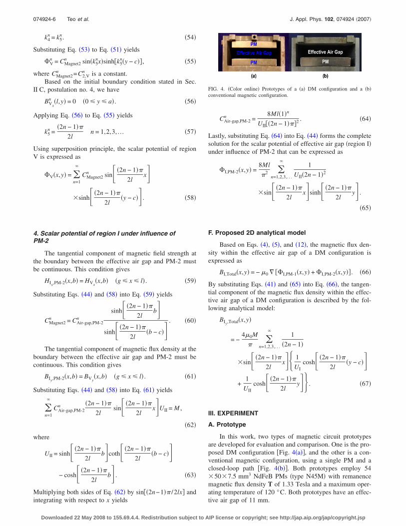
In this work, two types of magnetic circuit prototypesare developed for evaluation and comparison. One is the pro-posed DM configuration �Fig. 4�a��, and the other is a con-ventional magnetic configuration, using a single PM and aclosed-loop path �Fig. 4�b��. Both prototypes employ 54�50�7.5 mm3 NdFeB PMs �type N45M� with remanencemagnetic flux density T of 1.33 Tesla and a maximum oper-ating temperature of 120 °C. Both prototypes have an effec-tive air gap of 11 mm.

FIG. 4. �Color online� Prototypes of a �a� DM configuration and a �b�conventional magnetic configuration.



B. Experimental setup

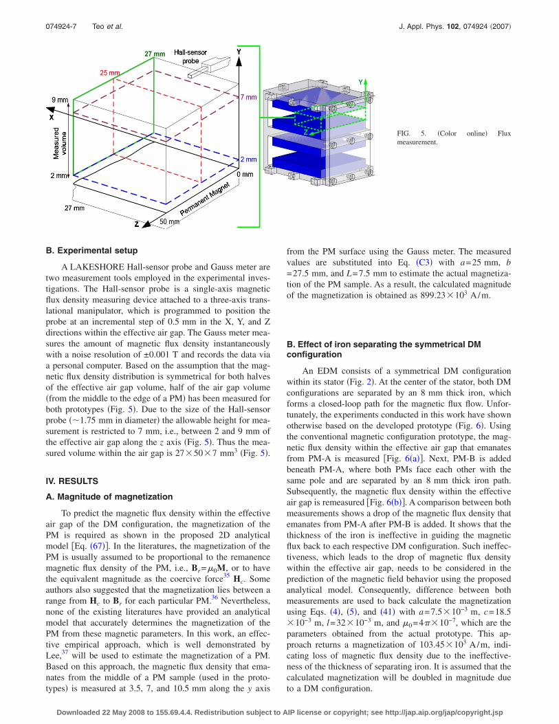
A LAKESHORE Hall-sensor probe and Gauss meter aretwo measurement tools employed in the experimental inves-tigations. The Hall-sensor probe is a single-axis magneticflux density measuring device attached to a three-axis trans-lational manipulator, which is programmed to position theprobe at an incremental step of 0.5 mm in the X, Y, and Zdirections within the effective air gap. The Gauss meter mea-sures the amount of magnetic flux density instantaneouslywith a noise resolution of ±0.001 T and records the data viaa personal computer. Based on the assumption that the mag-netic flux density distribution is symmetrical for both halvesof the effective air gap volume, half of the air gap volume�from the middle to the edge of a PM� has been measured forboth prototypes �Fig. 5�. Due to the size of the Hall-sensorprobe ��1.75 mm in diameter� the allowable height for mea-surement is restricted to 7 mm, i.e., between 2 and 9 mm ofthe effective air gap along the z axis �Fig. 5�. Thus the mea-sured volume within the air gap is 27�50�7 mm3 �Fig. 5�.

IV. RESULTS

A. Magnitude of magnetization

To predict the magnetic flux density within the effectiveair gap of the DM configuration, the magnetization of thePM is required as shown in the proposed 2D analyticalmodel �Eq. �67��. In the literatures, the magnetization of thePM is usually assumed to be proportional to the remanencemagnetic flux density of the PM, i.e., Br=�0M, or to havethe equivalent magnitude as the coercive force35 Hc. Someauthors also suggested that the magnetization lies between arange from Hc to Br for each particular PM.36 Nevertheless,none of the existing literatures have provided an analyticalmodel that accurately determines the magnetization of thePM from these magnetic parameters. In this work, an effec-tive empirical approach, which is well demonstrated byLee,37 will be used to estimate the magnetization of a PM.Based on this approach, the magnetic flux density that ema-nates from the middle of a PM sample �used in the proto-types� is measured at 3.5, 7, and 10.5 mm along the y axis

from the PM surface using the Gauss meter. The measuredvalues are substituted into Eq. �C3� with a=25 mm, b=27.5 mm, and L=7.5 mm to estimate the actual magnetiza-tion of the PM sample. As a result, the calculated magnitudeof the magnetization is obtained as 899.23�103 A/m.

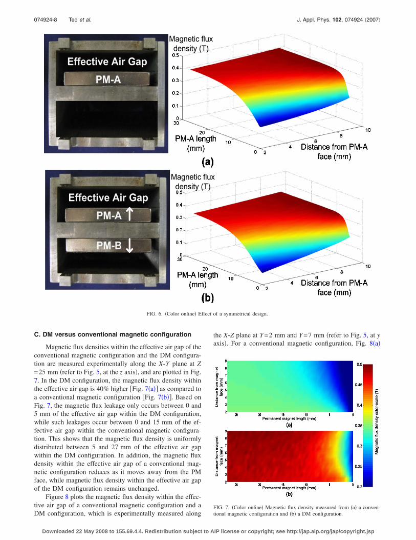
B. Effect of iron separating the symmetrical DMconfiguration

An EDM consists of a symmetrical DM configurationwithin its stator �Fig. 2�. At the center of the stator, both DMconfigurations are separated by an 8 mm thick iron, whichforms a closed-loop path for the magnetic flux flow. Unfor-tunately, the experiments conducted in this work have shownotherwise based on the developed prototype �Fig. 6�. Usingthe conventional magnetic configuration prototype, the mag-netic flux density within the effective air gap that emanatesfrom PM-A is measured �Fig. 6�a��. Next, PM-B is addedbeneath PM-A, where both PMs face each other with thesame pole and are separated by an 8 mm thick iron path.Subsequently, the magnetic flux density within the effectiveair gap is remeasured �Fig. 6�b��. A comparison between bothmeasurements shows a drop of the magnetic flux density thatemanates from PM-A after PM-B is added. It shows that thethickness of the iron is ineffective in guiding the magneticflux back to each respective DM configuration. Such ineffec-tiveness, which leads to the drop of magnetic flux densitywithin the effective air gap, needs to be considered in theprediction of the magnetic field behavior using the proposedanalytical model. Consequently, difference between bothmeasurements are used to back calculate the magnetizationusing Eqs. �4�, �5�, and �41� with a=7.5�10−3 m, c=18.5�10−3 m, l=32�10−3 m, and �0=4��10−7, which are theparameters obtained from the actual prototype. This ap-proach returns a magnetization of 103.45�103 A/m, indi-cating loss of magnetic flux density due to the ineffective-ness of the thickness of separating iron. It is assumed that thecalculated magnetization will be doubled in magnitude dueto a DM configuration.

FIG. 5. �Color online� Fluxmeasurement.



C. DM versus conventional magnetic configuration

Magnetic flux densities within the effective air gap of theconventional magnetic configuration and the DM configura-tion are measured experimentally along the X-Y plane at Z=25 mm �refer to Fig. 5, at the z axis�, and are plotted in Fig.7. In the DM configuration, the magnetic flux density withinthe effective air gap is 40% higher �Fig. 7�a�� as compared toa conventional magnetic configuration �Fig. 7�b��. Based onFig. 7, the magnetic flux leakage only occurs between 0 and5 mm of the effective air gap within the DM configuration,while such leakages occur between 0 and 15 mm of the ef-fective air gap within the conventional magnetic configura-tion. This shows that the magnetic flux density is uniformlydistributed between 5 and 27 mm of the effective air gapwithin the DM configuration. In addition, the magnetic fluxdensity within the effective air gap of a conventional mag-netic configuration reduces as it moves away from the PMface, while magnetic flux density within the effective air gapof the DM configuration remains unchanged.

Figure 8 plots the magnetic flux density within the effec-tive air gap of a conventional magnetic configuration and aDM configuration, which is experimentally measured along

the X-Z plane at Y =2 mm and Y =7 mm �refer to Fig. 5, at yaxis�. For a conventional magnetic configuration, Fig. 8�a�

FIG. 6. �Color online� Effect of a symmetrical design.

FIG. 7. �Color online� Magnetic flux density measured from �a� a conven-tional magnetic configuration and �b� a DM configuration.



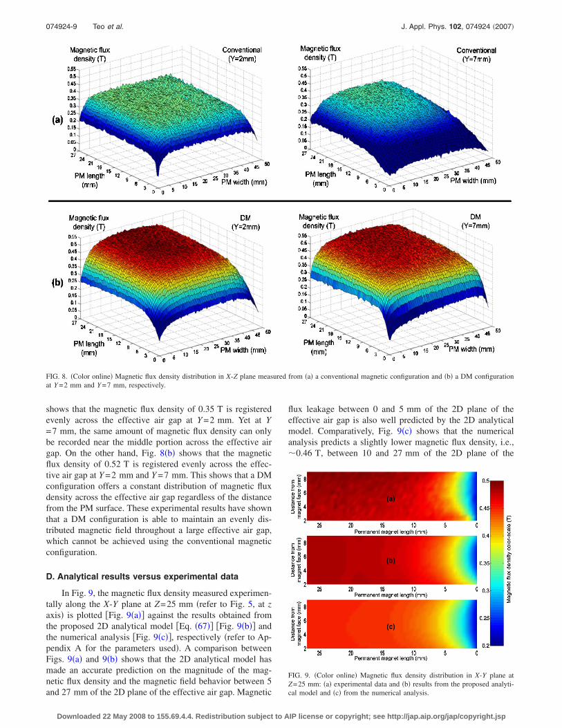
shows that the magnetic flux density of 0.35 T is registeredevenly across the effective air gap at Y =2 mm. Yet at Y=7 mm, the same amount of magnetic flux density can onlybe recorded near the middle portion across the effective airgap. On the other hand, Fig. 8�b� shows that the magneticflux density of 0.52 T is registered evenly across the effec-tive air gap at Y =2 mm and Y =7 mm. This shows that a DMconfiguration offers a constant distribution of magnetic fluxdensity across the effective air gap regardless of the distancefrom the PM surface. These experimental results have shownthat a DM configuration is able to maintain an evenly dis-tributed magnetic field throughout a large effective air gap,which cannot be achieved using the conventional magneticconfiguration.

D. Analytical results versus experimental data

In Fig. 9, the magnetic flux density measured experimen-tally along the X-Y plane at Z=25 mm �refer to Fig. 5, at zaxis� is plotted �Fig. 9�a�� against the results obtained fromthe proposed 2D analytical model �Eq. �67�� Fig. 9�b�� andthe numerical analysis �Fig. 9�c��, respectively �refer to Ap-pendix A for the parameters used�. A comparison betweenFigs. 9�a� and 9�b� shows that the 2D analytical model hasmade an accurate prediction on the magnitude of the mag-netic flux density and the magnetic field behavior between 5and 27 mm of the 2D plane of the effective air gap. Magnetic

flux leakage between 0 and 5 mm of the 2D plane of theeffective air gap is also well predicted by the 2D analyticalmodel. Comparatively, Fig. 9�c� shows that the numericalanalysis predicts a slightly lower magnetic flux density, i.e.,�0.46 T, between 10 and 27 mm of the 2D plane of the

FIG. 8. �Color online� Magnetic flux density distribution in X-Z plane measured from �a� a conventional magnetic configuration and �b� a DM configurationat Y =2 mm and Y =7 mm, respectively.

FIG. 9. �Color online� Magnetic flux density distribution in X-Y plane atZ=25 mm: �a� experimental data and �b� results from the proposed analyti-cal model and �c� from the numerical analysis.



effective air gap. A larger area of magnetic flux leakage de-rived from the numerical field solution also suggests that the2D analytical model offers a better prediction on the mag-netic flux distribution for a DM configuration.

The difference in the magnetic flux density between theanalytical and the experimental results is plotted in Fig. 10. Itshows that the 2D analytical model accurately predicts themagnitude of the magnetic flux density throughout the 2Dplane of the effective air gap with a deviation of ±0.02 T.Based on Fig. 10, a slight inaccuracy is found at the twocorners of the effective air gap, i.e., from 0 to 1 mm. Suchinaccuracies are accountable for as the actual PMs used inthe prototypes have fillet edges instead of sharp 90° edges,which are assumed during the formulation of the 2D analyti-cal model �refer to Fig. 4�. As a result, more magnetic fluxleakage is registered as projected at the two corner edges ofthe effective air gap in Fig. 9�a�.

The magnetic flux density measured experimentallyalong the Y-Z plane at X=27 mm �refer to Fig. 5, at x axis�is plotted in Fig. 11�a�. For comparison, the same analyticalresult obtained from the 2D analytical model is plotted inFig. 11�b�. It has shown that the 2D analytical model is alsoaccurate in predicting the magnitude of the magnetic fluxdensity along the Y-Z plane. Figure 12 plots the difference inthe magnetic flux density between the analytical and the ex-perimental results. It shows that the 2D analytical model can

accurately predict the magnitude of the magnetic flux densitythroughout the 2D plane of the effective air gap with a de-viation of ±0.02 T. Similarly, slight inaccurate predictionsoccur at the two corners of the effective air gap region due to

FIG. 10. �Color online� Difference in magnetic flux density between the results obtained from the proposed analytical model and the experiments �X-Y planeat Z=25 mm�.

FIG. 11. �Color online� Magnetic flux distribution in Y-Z plane at X=27 mm: �a� experimental data and �b� results from the proposed analyticalmodel.



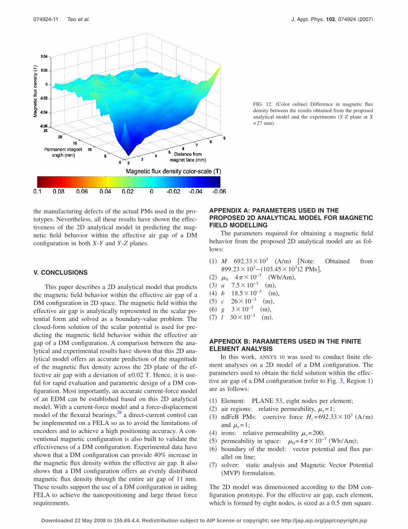
the manufacturing defects of the actual PMs used in the pro-totypes. Nevertheless, all these results have shown the effec-tiveness of the 2D analytical model in predicting the mag-netic field behavior within the effective air gap of a DMconfiguration in both X-Y and Y-Z planes.

V. CONCLUSIONS

This paper describes a 2D analytical model that predictsthe magnetic field behavior within the effective air gap of aDM configuration in 2D space. The magnetic field within theeffective air gap is analytically represented in the scalar po-tential form and solved as a boundary-value problem. Theclosed-form solution of the scalar potential is used for pre-dicting the magnetic field behavior within the effective airgap of a DM configuration. A comparison between the ana-lytical and experimental results have shown that this 2D ana-lytical model offers an accurate prediction of the magnitudeof the magnetic flux density across the 2D plane of the ef-fective air gap with a deviation of ±0.02 T. Hence, it is use-ful for rapid evaluation and parametric design of a DM con-figuration. Most importantly, an accurate current-force modelof an EDM can be established based on this 2D analyticalmodel. With a current-force model and a force-displacementmodel of the flexural bearings,28 a direct-current control canbe implemented on a FELA so as to avoid the limitations ofencoders and to achieve a high positioning accuracy. A con-ventional magnetic configuration is also built to validate theeffectiveness of a DM configuration. Experimental data haveshown that a DM configuration can provide 40% increase inthe magnetic flux density within the effective air gap. It alsoshows that a DM configuration offers an evenly distributedmagnetic flux density through the entire air gap of 11 mm.These results support the use of a DM configuration in aidingFELA to achieve the nanopositioning and large thrust forcerequirements.

APPENDIX A: PARAMETERS USED IN THEPROPOSED 2D ANALYTICAL MODEL FOR MAGNETICFIELD MODELLING

The parameters required for obtaining a magnetic fieldbehavior from the proposed 2D analytical model are as fol-lows:

�1� M 692.33�103 �A/m� �Note: Obtained from899.23�103− �103.45�103�2 PMs�,

�2� �0 4��10−7 �Wb/Am�,�3� a 7.5�10−3 �m�,�4� b 18.5�10−3 �m�,�5� c 26�10−3 �m�,�6� g 3�10−3 �m�,�7� l 30�10−3 �m�.

APPENDIX B: PARAMETERS USED IN THE FINITEELEMENT ANALYSIS

In this work, ANSYS 10 was used to conduct finite ele-ment analyses on a 2D model of a DM configuration. Theparameters used to obtain the field solution within the effec-tive air gap of a DM configuration �refer to Fig. 3, Region 1�are as follows:

�1� Element: PLANE 53, eight nodes per element;�2� air regions: relative permeability, �r=1;�3� ndFeB PMs: coercive force Hc=692.33�103 �A/m�

and �r=1;�4� irons: relative permeability �r=200;�5� permeability in space: �0=4��10−7 �Wb/Am�;�6� boundary of the model: vector potential and flux par-

allel on line;�7� solver: static analysis and Magnetic Vector Potential

�MVP� formulation.

The 2D model was dimensioned according to the DM con-figuration prototype. For the effective air gap, each element,which is formed by eight nodes, is sized as a 0.5 mm square.

FIG. 12. �Color online� Difference in magnetic fluxdensity between the results obtained from the proposedanalytical model and the experiments �Y-Z plane at X=27 mm�.



The magnetic flux density By of each element is obtained byaveraging the values of all the nodes that form the element.

APPENDIX C: A CONVENTIONAL MAGNETIC FIELDMODEL

Currently the magnetic field of a PM is commonly ana-lyzed using an analytical model that describes a PM withmagnetic charge. Based on this principle, Furlani34 made acomprehensive derivation of this model, and the scalar po-tential that is used to describe the magnetic field of the abovePM can be expressed as

� = −1

4��

V� � �� · M�x��

�x − x��dv� +

1

4�

S

M�x�� · n

�x − x��ds�,

�C1�

where the solution gives a sum of the magnetic charge vol-ume V and the surface S confining it. In addition, x is thevector of the observation point, x� is the vector of sourcepoint,�� operates on the primed coordinates, and n is theoutward unit normal to the surface.

For 1D analysis of the magnetic flux density above aPM, it is assumed that the magnetization M=My→−� ·M=0. Using Eqs. �4� and �C1�, x=y�y and x�=x�x+z�z, themagnetic flux density along the y axis for a DM configura-tion is expressed as

ByTotal�d� = By

PM−1�d� + ByPM−2�d − g� , �C2�

where

By�� =�0M

��tan−1 �� + L��a2 + b2 + �� + L�2

ab

− tan−1� p�a + b + �

ab�� , �C3�

with a=half the width of magnet, b=half the length of mag-net, L=thickness of magnet, and � represents the distancefrom the surface of PM-1, i.e., d, or from the surface PM-2,i.e., d−g �where g=height of air gap�.

1H. J. Mamin, D. W. Abraham, E. Ganz, and J. Clark, Rev. Sci. Instrum. 56,2168 �1985�.

2K. Fite and M. Goldfarb, IEEE International Conference on Robotics andAutomation �IEEE, New York, 1999�, pp. 2122–2127.

3L. Dong, F. Arai, and T. Fukuda, International Symposium on Micro-mechatronics and Human Science, March 2000, pp. 151–156.

4L. W. Kimball, D. D. Tsai, and J. Maloney, ASME Design EngineeringTechnical Conferences, 2000.

5Y. Sun, D. Piyabongkarn, A. Sezen, B. J. Nelson, R. Rajamani, R. Schoch,and D. P. Potasek, 2002 IEEE/RSJ International Conference on Intelli-gence Robots and Systems, EPFL, Lausanne, Switzerland, October 2002�IEEE, New York, 2002�, pp. 1796–1801.

6B. Zhang and Z. Zhu, IEEE/ASME Trans. Mechatron. 2, 22 �1997�.7K. K. Tan, T. H. Lee, and H. X. Zhou, IEEE/ASME Trans. Mechatron. 6,428 �2001�.

8U. Kenji, Piezoelectric Actuator and Ultrasonic Motors �Kluwer-Academic, Dordrecht, 1997�.

9T. G. King, Precis. Eng. 12, 131 �1990�.10P. J. Falter, Diamond Turning of Nonrotationally Symmetric Surfaces

�North Carolina State University, Raleigh, NC, 1990�.11D. L. Trumper, Ph.D. Thesis, Massachusetts Institute of Technology, 1990.12T. Higuchi and T. Yamaguchi, J. Jpn. Soc. Precis. Eng. 59, 37 �1993�.13M. L. Holmes, M.S. thesis University of North Carolina, 1994.14S. L. Ludwick, D. L. Trumper, and M. L. Holmes, IEEE Trans. Control

Syst. Technol. 4, 553 �1996�.15K.-S. Chen, D. L. Trumper, and S. T. Smith, Precis. Eng. 26, 355 �2002�.16K.-S. Chen and C.-C. Ho, Precis. Eng. 28, 106 �2004�.17K. Takahara, 22nd Aerospace Mechanism Symposium, May 1988 �unpub-

lished�, pp. 133–147.18K. Park, K.-B. Choi, S.-H. Kim, and Y. K. Kwak, IEEE Trans. Magn. 32,

208 �1996�.19W.-J. Kim, Ph.D. thesis, Massachusetts Institute of Technology, 1997.20W.-J. Kim and D. L. Trumper, Precis. Eng. 22, 66 �1998�.21M. Holmes, R. Hocken, and D. Trumper, Precis. Eng. 24, 191 �2000�.22W.-J. Kim and H. Maheshwari, Proceedings of the American Control Con-

ference, 2002, pp. 4279–4284, Vol. 5.23S. Verma, W.-J. Kim, and J. Gu, IEEE/ASME Trans. Mechatron. 9, 384

�2004�.24S. Mori, T. Hoshino, G. Obinata, and K. Ouchi, IEEE Trans. Magn. 39,

812 �2003�.25S. Fukada and T. Shibuya, Third Euspen International Conference, Eind-

hoven, The Netherland, May 2002, pp. 171–174.26B. Sprenger, O. Binzel, and R. Siegwart, Fourth International Conference

on Motion and Vibration Control �MOVIC 1998�, Zurich, 1998, pp. 1145–1150.

27B. Sprenger, IEEE/ASME International Conference on Advanced Intelli-gent Mechatronics ’97 �IEEE, New York, 1997�, p. 63.

28T. J. Teo, I.-M. Chen, G. L. Yang, and W. Lin, Proceedings of the Inter-national Conference on Robotics and Automation Roma, Italy.

29G. Yang and T. J. Teo, Intellectual Property Office of Singapore �A-STAR,Singapore, 2005�.

30T. J. Teo, I.-M. Chen, G. L. Yang, and W. Lin, Romansy 16 �Springer, NewYork, 2006�, pp. 317–378.

31E. P. Furlani, IEEE Trans. Magn. 28, 2061 �1992�.32E. P. Furlani, IEEE Trans. Magn. 30, 3660 �1994�.33J. Wang, G. W. Jewell, and D. Howe, J. Appl. Phys. 81, 4266 �1997�.34E. P. Furlani, Permanent Magnet and Electromechanical Devices �Aca-

demic, New York, 2001�.35J. R. Brauer, L. A. Larkin, and V. D. Overbye, J. Appl. Phys. 55, 2138

�1984�.36J. K. Lee and T. S. Lewis, J. Appl. Phys. 70, 6615 �1991�.37J. K. Lee, IEEE Trans. Magn. 28, 3021 �1992�.



Documents

Magnetic field modeling of a dual-magnet …...Magnetic field modeling of a dual-magnet configuration Tat Joo Teo a and I-Ming Chen School of Mechanical & Aerospace Engineering,