See discussions, stats, and author profiles for this publication at: https://www.researchgate.net/publication/237020586

Magnetic properties of unrusted steel drums from laboratory and field-magnetic

measurements

Article  in  Geophysics · September 1996

DOI: 10.1190/1.1444056

CITATIONS

24

READS

79

1 author:

Some of the authors of this publication are also working on these related projects:

An informal gravity and magnetic community effort to advance data bases, modeling, and analysis efforts View project

Dhananjay Ravat

Earth & Environmental Sciences and

125 PUBLICATIONS   2,002 CITATIONS   

SEE PROFILE

All content following this page was uploaded by Dhananjay Ravat on 29 May 2014.

The user has requested enhancement of the downloaded file.

GEOPHYSICS, VOL. 61, NO. 5 (SEPTEMBER-OCTOBER 1996); P. 1325-1335,7 FIGS., 4 TABLES.

Magnetic properties of unrusted steel drums fromlaboratory and field-magnetic measurements

Dhananjay Ravat*

ABSTRACT

Laboratory-derived magnetic properties from sam-ples of steel drums appear to be lower than bulkmagnetic properties required to produce observed mag-netic anomalies over the same drums. The origin ofthis discrepancy is perhaps in the shape demagneti-zation experienced by samples used in the laboratorystudy. Laboratory observations of magnetic susceptibil-ity in different directions suggest that the demagne-tization mechanism may have significantly attenuatedthe laboratory-derived magnetization values from smallsamples of drums. Field observations and computer mod-eling indicate that even though the effect of demagneti-zation is important for drum-shaped objects, demagne-tization is less pronounced in the shape of the drum thanin the samples cut for laboratory measurements. There-fore, laboratory-derived magnetizations from samples ofsteel drums cannot be used to model magnetic anoma-lies of steel drums. If laboratory-derived magnetizationswere used to model steel drums, the models would under-estimate the resulting magnetic anomalies considerably

and, in turn, would overestimate the number of burieddrums at an environmental investigation site. Apparentbulk magnetization values for unrusted vertically ori-ented 55 and 30 gallon drums have been calculated (i.e.,the values corrected for the effect of shape demagneti-zation of the drums). These range from to ~125 SIunits to cgs units) for volume susceptibility andfrom ~325 to ~2750 A/m (-0.325 to emu/cm3)for remanent magnetization (based on eight 55 gallonand four 30 gallon drums). Further deviations in thesevalues could arise from the type and thickness of thesteel and variations in manufacturing conditions affect-ing magnetizations. From the point of view of model-ing the drums, at most source-to-observation distancesapplicable to environmental investigations, the equiva-lent source method is able to approximate the observedanomalies of steel drums better than the 3-D modelingmethod. With two years of rusting, magnetic anoma-lies of some of the drums have reduced, while in otherdrums, they have slightly increased. The overall magneticchanges caused by rusting appear to be more complexthan anticipated, at least in the initial phase of rusting.

INTRODUCTION forward using either horizontal [e.g., straight-slope or similarmethods, see Skilbrei (1993); rules of thumb, e.g., Hinze (1990)]

Detection and precise location of buried ferromagnetic ob- or vertical [e.g., Euler deconvolution, Thompson, (1982);jects and estimation of the type and quantity of the objects Ravat (1994)] gradient-based techniques. While the estimationare becoming increasingly important in environmental inves- of the type of source (e.g., steel drums, steel tanks, pipelines,tigations worldwide. The magnetic method is very useful, in etc.) can be made in many circumstances by observing anomalycases where the signal-to-noise ratio of the magnetic anoma-patterns (also, many times, the type of the object is known alies is high, for detecting horizontal (x, y) locations of isolated priori), judging the quantity of such closely spaced objects re-buried ferromagnetic objects (assuming that maxima/minima quires that the object(s) be modeled because magnetic anoma-shifts because of the inclination and declination of the Earth’s lies from nearby sources merge into a single anomaly at mostfield orientation and because of the direction of the total mag- practical source-to-observation distances. At present, it is pos-netization vector are taken into account). Finding the depth of sible to use a forward or an elementary inverse modelingcompact objects within an acceptable error bound is straight- approach to estimate approximately (approximately, because

Manuscript received by the Editor April 17,1995; revised manuscript received November 20,1995.*Department of Geology, MS 4324, Southern Illinois University at Carbondale, Carbondale, IL 62901.© 1996 Society of Exploration Geophysicists. All rights reserved.

1325

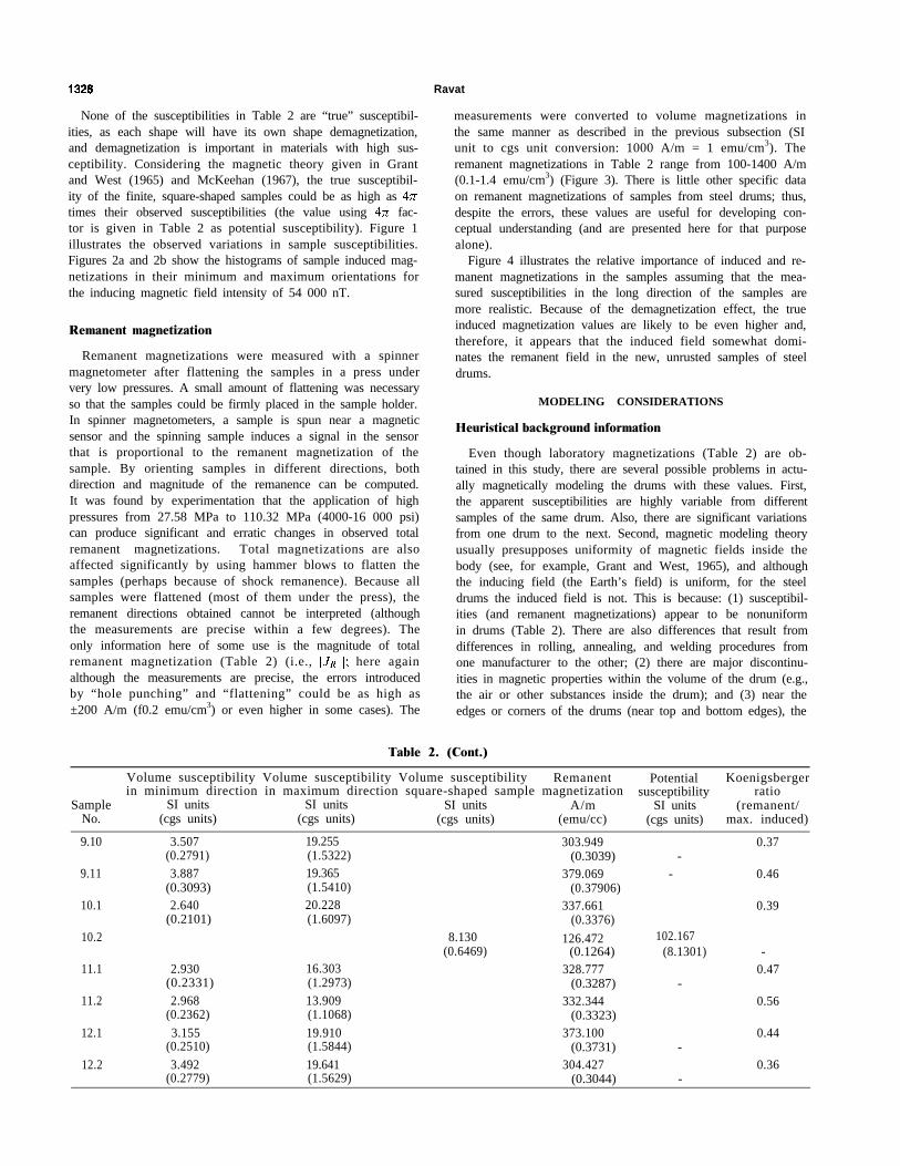
1326

of potential-field nonuniqueness and also because anomaliescaused by different size drums have significantly differentamplitudes) the number of drums and their locations in caseswhere the signal-to-noise ratio is high. What is lacking is knowl-edge of the range of values of susceptibility and the remanentmagnetization to be considered in such modeling.

In this study, first, laboratory and field magnetizations of new(unrusted) steel drums are determined. The laboratory andfield-derived magnetizations and the observed and computedmagnetic anomalies are then compared to investigate possiblecorrelations and discrepancies. A modeling comparison is alsomade between the equivalent source method and a 3-D mod-eling method to determine their usefulness in environmentalinvestigations. Common definitions of various magnetic prop-erties used in this paper and additional definitions used herefor the purpose of clarity are given in Table 1.

LABORATORY MEASUREMENTS

For measuring susceptibility and remanent magnetizations,36 samples (0.0254 m or 1 in. diameter) were extracted from12 steel drums using an industrial hole punch. This is probablynot the best method for preserving the original magnetizations(use of heavy duty shears may be the best method if smallflat pieces of a drum can be extracted), but it is probably theleast destructive method of extracting samples, i.e., without de-stroying the shape of the drum. The drawback of this method isthat some pressure is applied while removing samples, and thepressure could change magnetizations. Using the hole punch,pressure can be increased slowly and, therefore, no shock mag-netization is expected during the sample extraction.

Ravat

Susceptibility and induced magnetization

Susceptibility measurements were performed on aBartington susceptibility bridge where samples are placed in acoil in an inductor-resistor-capacitor (LRC) circuit, the changesin the current being proportional to the magnetic susceptibilityof the sample. The measurements were made at 79.577 A/m(1 Oe) inducing field intensity and were found to be precise toabout SI units cgs units); the precision of theobservations is about two orders of magnitude better than thelowest observed susceptibility. The measurements were madein a cgs system of units, normalized to weight in grams, andconverted to volume susceptibility in cgs units by using densityof steel = 7.874 Mg/m3 or g/cm3) (susceptibility in SI unitsis times the susceptibility in cgs units). Most samples usedfor susceptibility measurements were long in one dimension(length/width -3). Therefore, the susceptibility measurementswere made in steps, by rotating the sample orientation withrespect to the plane of the coil on the susceptibility bridge. Themaximum values were observed when the long axis of the sam-ple was perpendicular to the plane of the coil (i.e., along theaxis of the coil, or along the inducing field) and the minimumvalues were observed when the long axis of the sample wasparallel to the plane of the coil (Table 2). These observationsare consistent with the supposition of magnetic anisotropy,i.e., the tendency to reorient the susceptibility into the planeor the axis of the long dimension of an object (Breiner, 1973;called “aeolotropy” in Grant and West, 1965). A few sampleswere cut further into square shapes. Their observations did notdepend significantly on the orientation, but their magnitudeswere only a little above the minimum observed values.

Table 1. Glossary of specialized magnetic terms (*denotes important caveats).

Effective susceptibilityEffect of combined induced and remanent magnetization translated into susceptibility assuming that remanent magnetizationlies in the same direction as the inducing field. (*This property is computed from field observations, and may be used onlywhen either remanent magnetization is negligible or lies in the same direction as the inducing field.)

Effective apparent susceptibilityEffective susceptibility as observed from a sample of a particular shape and size (e.g., reduction in the effective susceptibilitybecause of demagnetization is taken into account here). (*Same as above.)

Bulk magnetizationCombined induced and remanent magnetization vector as observed by magnetometers some distance away from an objectof a particular shape and size.

Apparent bulk (total) magnetizationCombined induced and remanent magnetization vector as observed by magnetometers some distance away from an objectof a particular shape and size. (*A calculated quantity from field measurements. This quantity takes into account theeffective reduction in bulk magnetization because of demagnetization in one step and, thus, eliminates the need forcomplicated iterative forward modeling of demagnetization for all practical purposes.)

Apparent bulk induced magnetizationThe induced part of the apparent bulk magnetization

Apparent bulk susceptibilitySusceptibility calculated from the apparent bulk induced magnetization

Apparent bulk remanent magnetizationThe remanent part of the apparent bulk magnetization

Equivalent source (total/induced/remanent) magnetizationNumerical best-fit magnetization that would be required to approximate (all of/induced part of/remanent part of) theobserved magnetic anomaly by a magnetic dipole placed at a specific location. (*This quantity is not real. It is computedfrom the inversion of the field data after first splitting the inverted dipole moment vector into its component-inducedand remanent vectors using either 3 or 4 orientation field observations as discussed in the text andthen normalizing the magnitudes of the vectors by a relatively small arbitrary volume.)

Equivalent source susceptibilityNumerical best-fit susceptibility that would be required to approximate only the induced part of the observed magneticanomaly by a magnetic dipole placed at a specific location. (*Same as above.)

Magnetic Properties of Steel Drums 1327

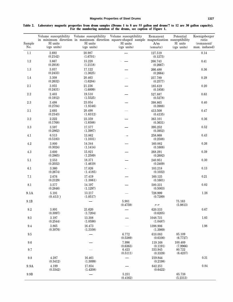
Table 2. Laboratory magnetic properties from drum samples (Drums 1 to 8 are 55 gallon and drums�? to 12 are 30 gallon capacity).For the numbering notation of the drums, see caption of Figure 1.

Volume susceptibility Volume susceptibility Volume susceptibility Remanent Potential Koenigsbergerin minimum direction in maximum direction square-shaped sample magnetization susceptibility ratio

Sample SI units SI units SI units A/m SI units (remanent/No. (cgs units) (cgs units) (cgs units) (emu/cc) (cgs units) max. induced)

1.1

1.2

1.3

1.4

2.1

2.2

2.3

3.1

3.2

3.3

4.1

4.2

4.3

5.1

6.1

7.1

8.1

9.1A

9.1B

9.2

9.3

9.4

9.5

9.6

9.7

9.8

9.9A

9.9B

2.692 20.987(0.2142) (1.6701)3.667 15.228

(0.2918) (1.2118)3.057 17.122

(0.2433) (1.3625)3.308 20.463

(0.2632) (1.6284)3.055 21.236

(0.2431) (1.6899)2.403 19.510

(0.1912) (1.5525)3.498 23.054

(0.2784) (1.8346)2.693 20.498

(0.2143) (1.6312)2.222 23.359

(0.1768) (1.8588)3.597 17.577

(0.2862) (1.3987)6.513 13.862

(0.5183) (1.1031)3.800 14.344

(0.3024) (1.1414)3.600 15.821

(0.2865) (1.2589)2.553 18.371

(0.2032) (1.4619)3.360 17.826

(0.2674) (1.4185)2.676 17.419

(0.2129) (1.3861)3.577 14.197

(0.2846) (1.1297)5.191 13.217

(0.413 (1.0517)

3.891 21.620(0.3097) (1.7204)3.197 13.308

(0.2544) (1.0590)3.865 16.473

(0.3076) (1.3108)

4.287 16.461(0.3412) (1.3099)4.199 17.854

(0.3342) (1.4208)

5.981(0.4759)

6.772(0.5389)7.996

(0.6363)6.423

(0.5111)

5.231 65.738(0.4162) (5.2313)

127.519(0.1275)

266.743(0.2667)

266.488(0.2664)

257.789(0.2577)

185.619(0.1856)

527.887(0.5278)

398.865(0.3988)

413.508(0.4135)

363.101(0.3631)

395.252(0.3952)

258.868(0.2588)

160.882(0.1608)

268.291(0.2682)

240.951(0.2409)

103.218(0.1032)

160.125(0.1601)

500.331(0.5003)

728.999(0.7289)

620.533

(0.6205)1048.721

(1.0487)1398.906

(1.3989)610.083

(0.6100)119.168

(0.1191)333.945

(0.3339)219.844

(0.2198)642.251

(0.6422)

75.163(5.9813)

85.109(6.7727)

100.489(7.9966)80.722(6.4237)

0.14

0.41

0.36

0.29

0.20

0.63

0.40

0.47

0.36

0.52

0.43

0.26

0.39

0.30

0.13

0.21

0.82

1.28

0.67

1.83

1.98

0.31

0.84

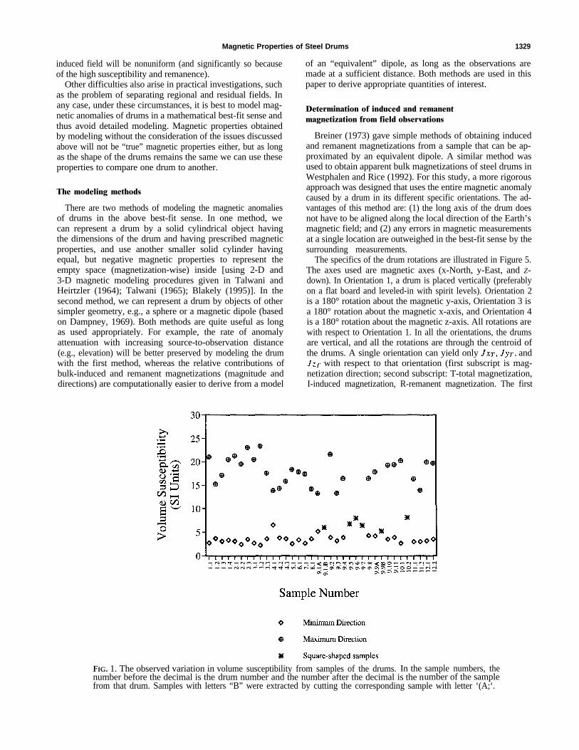
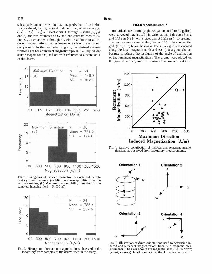
None of the susceptibilities in Table 2 are “true” susceptibil-ities, as each shape will have its own shape demagnetization,and demagnetization is important in materials with high sus-ceptibility. Considering the magnetic theory given in Grantand West (1965) and McKeehan (1967), the true susceptibil-ity of the finite, square-shaped samples could be as high as times their observed susceptibilities (the value using fac-tor is given in Table 2 as potential susceptibility). Figure 1illustrates the observed variations in sample susceptibilities.Figures 2a and 2b show the histograms of sample induced mag-netizations in their minimum and maximum orientations forthe inducing magnetic field intensity of 54 000 nT.

Remanent magnetization

Remanent magnetizations were measured with a spinnermagnetometer after flattening the samples in a press undervery low pressures. A small amount of flattening was necessaryso that the samples could be firmly placed in the sample holder.In spinner magnetometers, a sample is spun near a magneticsensor and the spinning sample induces a signal in the sensorthat is proportional to the remanent magnetization of thesample. By orienting samples in different directions, bothdirection and magnitude of the remanence can be computed.It was found by experimentation that the application of highpressures from 27.58 MPa to 110.32 MPa (4000-16 000 psi)can produce significant and erratic changes in observed totalremanent magnetizations. Total magnetizations are alsoaffected significantly by using hammer blows to flatten thesamples (perhaps because of shock remanence). Because allsamples were flattened (most of them under the press), theremanent directions obtained cannot be interpreted (althoughthe measurements are precise within a few degrees). Theonly information here of some use is the magnitude of totalremanent magnetization (Table 2) (i.e., here againalthough the measurements are precise, the errors introducedby “hole punching” and “flattening” could be as high as±200 A/m (f0.2 emu/cm3) or even higher in some cases). The

Ravat

measurements were converted to volume magnetizations inthe same manner as described in the previous subsection (SIunit to cgs unit conversion: 1000 A/m = 1 emu/cm3). Theremanent magnetizations in Table 2 range from 100-1400 A/m(0.1-1.4 emu/cm3) (Figure 3). There is little other specific dataon remanent magnetizations of samples from steel drums; thus,despite the errors, these values are useful for developing con-ceptual understanding (and are presented here for that purposealone).

Figure 4 illustrates the relative importance of induced and re-manent magnetizations in the samples assuming that the mea-sured susceptibilities in the long direction of the samples aremore realistic. Because of the demagnetization effect, the trueinduced magnetization values are likely to be even higher and,therefore, it appears that the induced field somewhat domi-nates the remanent field in the new, unrusted samples of steeldrums.

MODELING CONSIDERATIONS

Heuristical background information

Even though laboratory magnetizations (Table 2) are ob-tained in this study, there are several possible problems in actu-ally magnetically modeling the drums with these values. First,the apparent susceptibilities are highly variable from differentsamples of the same drum. Also, there are significant variationsfrom one drum to the next. Second, magnetic modeling theoryusually presupposes uniformity of magnetic fields inside thebody (see, for example, Grant and West, 1965), and althoughthe inducing field (the Earth’s field) is uniform, for the steeldrums the induced field is not. This is because: (1) susceptibil-ities (and remanent magnetizations) appear to be nonuniformin drums (Table 2). There are also differences that result fromdifferences in rolling, annealing, and welding procedures fromone manufacturer to the other; (2) there are major discontinu-ities in magnetic properties within the volume of the drum (e.g.,the air or other substances inside the drum); and (3) near theedges or corners of the drums (near top and bottom edges), the

Table 2. (Cont.)

Volume susceptibility Volume susceptibility Volume susceptibility Remanent Potential Koenigsbergerin minimum direction in maximum direction square-shaped sample magnetizationsusceptibility ratio

Sample SI units SI units SI units A/m SI units (remanent/No. (cgs units) (cgs units) (cgs units) (emu/cc) (cgs units) max. induced)

9.10 3.507 19.255 303.949 0.37(0.2791) (1.5322) (0.3039) -

9.11 3.887(0.3093)

10.1 2.640(0.2101)

10.2

11.1 2.930(0.2331)

11.2 2.968

19.365(1.5410)20.228(1.6097)

8.130(0.6469)

16.303(1.2973)13.909

379.069 - 0.46(0.37906)

337.661 0.39(0.3376)

102.167126.472-(0.1264) (8.1301)

328.777(0.3287) -

0.47

332.344 0.56(0.2362) (1.1068) (0.3323)

12.1 3.155 19.910 373.100 0.44(0.2510) (1.5844) (0.3731) -

12.2 3.492 19.641 304.427 0.36(0.2779) (1.5629) (0.3044) -

Magnetic Properties of Steel Drums 1329

induced field will be nonuniform (and significantly so becauseof the high susceptibility and remanence).

Other difficulties also arise in practical investigations, suchas the problem of separating regional and residual fields. Inany case, under these circumstances, it is best to model mag-netic anomalies of drums in a mathematical best-fit sense andthus avoid detailed modeling. Magnetic properties obtainedby modeling without the consideration of the issues discussedabove will not be “true” magnetic properties either, but as longas the shape of the drums remains the same we can use theseproperties to compare one drum to another.

The modeling methods

There are two methods of modeling the magnetic anomaliesof drums in the above best-fit sense. In one method, wecan represent a drum by a solid cylindrical object havingthe dimensions of the drum and having prescribed magneticproperties, and use another smaller solid cylinder havingequal, but negative magnetic properties to represent theempty space (magnetization-wise) inside [using 2-D and3-D magnetic modeling procedures given in Talwani andHeirtzler (1964); Talwani (1965); Blakely (1995)]. In thesecond method, we can represent a drum by objects of othersimpler geometry, e.g., a sphere or a magnetic dipole (basedon Dampney, 1969). Both methods are quite useful as longas used appropriately. For example, the rate of anomalyattenuation with increasing source-to-observation distance(e.g., elevation) will be better preserved by modeling the drumwith the first method, whereas the relative contributions ofbulk-induced and remanent magnetizations (magnitude anddirections) are computationally easier to derive from a model

of an “equivalent” dipole, as long as the observations aremade at a sufficient distance. Both methods are used in thispaper to derive appropriate quantities of interest.

Determination of induced and remanentmagnetization from field observations

Breiner (1973) gave simple methods of obtaining inducedand remanent magnetizations from a sample that can be ap-proximated by an equivalent dipole. A similar method wasused to obtain apparent bulk magnetizations of steel drums inWestphalen and Rice (1992). For this study, a more rigorousapproach was designed that uses the entire magnetic anomalycaused by a drum in its different specific orientations. The ad-vantages of this method are: (1) the long axis of the drum doesnot have to be aligned along the local direction of the Earth’smagnetic field; and (2) any errors in magnetic measurementsat a single location are outweighed in the best-fit sense by thesurrounding measurements.

The specifics of the drum rotations are illustrated in Figure 5.The axes used are magnetic axes (x-North, y-East, and Z-down). In Orientation 1, a drum is placed vertically (preferablyon a flat board and leveled-in with spirit levels). Orientation 2is a 180° rotation about the magnetic y-axis, Orientation 3 isa 180° rotation about the magnetic x-axis, and Orientation 4is a 180° rotation about the magnetic z-axis. All rotations arewith respect to Orientation 1. In all the orientations, the drumsare vertical, and all the rotations are through the centroid ofthe drums. A single orientation can yield only and

with respect to that orientation (first subscript is mag-netization direction; second subscript: T-total magnetization,I-induced magnetization, R-remanent magnetization. The first

FIG. 1. The observed variation involume susceptibility from samples of the drums.In thesample numbers, thenumber before the decimal is the drum number and the number after the decimal is the number of the samplefrom that drum. Samples with letters “B” were extracted by cutting the corresponding sample with letter ‘(A;‘.

1330

subscript is omitted when the total magnetization of each kindis considered, i.e., = total induced magnetization = sqrt

+ + Orientations 1 through 3 yield JXI, Jyi,and J.g and two estimates of JZR and one estimate each of JXR

and JYR. Orientations 1 through 4 yield, in addition to all in-duced magnetizations, two estimates of each of the remanentcomponents. In the computer program, the derived magne-tizations are for equivalent magnetic dipoles (i.e., equivalentsource magnetizations) and are with reference to Orientation 1of the drums.

FIG. 2. Histograms of induced magnetizations obtained by lab-oratory measurements. (a) Minimum susceptibility directionof the samples; (b) Maximum susceptibility direction of thesamples. Inducing field = 54000 nT.

FIG. 3. Histogram of remanent magnetizations observed in thelaboratory from samples of the drums used in the study.

FIELD MEASUREMENTS

Individual steel drums (eight 5.5 gallon and four 30 gallon)were surveyed magnetically in Orientations 1 through 3 in agrid 14.63 m (48 ft) on its sides and at 1.219 m (4 ft) spacing.The drums were centered at the (7.62 m, 7.62 m) location on thegrid, (0 m, 0 m) being the origin. The survey grid was orientedalong the local magnetic north and east (not a good choice,because it reduced the resolution of the angle of declinationof the remanent magnetization). The drums were placed onthe ground surface, and the sensor elevation was 2.438 m

FIG. 4. Relative contribution of induced and remanent magne-tizations as observed from laboratory measurements.

FIG. 5. Illustration of drum orientations used to determine in-duced and remanent magnetizations from field magnetic mea-surements. The axes shown are magnetic axes (i.e., x-North;y-East; z-down). In all orientations, the drums are vertical.

Magnetic Properties of Steel Drums 1331

(8 ft) above the ground (the sensor staff came in segments of0.6096 m (2 ft), hence the choice of feet as the distance unit).Five drums (one 55 gallon and all 30 gallon) were also surveyedin Orientation 4. The survey was conducted during April-May1993 on a site provided by the College of Agriculture at South-ern Illinois University at Carbondale. By prior magnetic sur-veying, the site was deemed to be magnetically “clean.” Thearea was also surveyed with the above specifications in theabsence of drums. Residual magnetic anomalies of each ofthe drums in the above orientations were obtained after cor-rections for temporal variations by reoccupying a base station(surveys were abandoned when large, erratic temporal varia-tions were observed) and after removing the field without thedrums (i.e., the regional). No latitudinal correction was appliedas the area covers only 14.63 m in the North-South direction.

THE MODELING

Equivalent source modeling

In equivalent source modeling, placement of an equivalentmagnetic dipole is of importance because we want to fit the ob-served anomalies as well as possible. The horizontal locationof the dipole should obviously be the horizontal center of thedrum. The vertical location of the dipole that numerically fitsthe anomaly the best was determined from Euler’s equationassuming the anomaly attenuation rate of 3, which is the the-oretical anomaly attenuation rate for a magnetic dipole (e.g.,Ravat, 1994). The average vertical location for the equivalent

dipole for 55 gallon drums was 0.183 m (0.6 ft) and for 30 gal-lon drums was 0.122 m (0.4 ft), both above the ground surface;hence, for all the drums, the equivalent dipoles were placed at0.1525 m (0.5 ft) above the ground surface. The drums in thisexperiment were always kept in Orientation 1, except whenthe measurements in the other orientations were carried out.Thus, in this study, some of the viscous magnetic effects willcontribute toward the derived remanent magnetization vectorand some toward the induced magnetization vector (see alsothe discussion section).

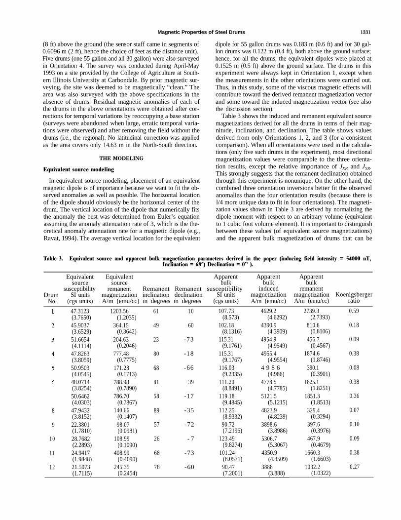
Table 3 shows the induced and remanent equivalent sourcemagnetizations derived for all the drums in terms of their mag-nitude, inclination, and declination. The table shows valuesderived from only Orientations 1, 2, and 3 (for a consistentcomparison). When all orientations were used in the calcula-tions (only five such drums in the experiment), most directionalmagnetization values were comparable to the three orienta-tion results, except the relative importance of JXR and JYR.This strongly suggests that the remanent declination obtainedthrough this experiment is nonunique. On the other hand, thecombined three orientation inversions better fit the observedanomalies than the four orientation results (because there isl/4 more unique data to fit in four orientations). The magneti-zation values shown in Table 3 are derived by normalizing thedipole moment with respect to an arbitrary volume (equivalentto 1 cubic foot volume element). It is important to distinguishbetween these values (of equivalent source magnetizations)and the apparent bulk magnetization of drums that can be

Table 3. Equivalent source and apparent bulk magnetization parameters derived in the paper (inducing field intensity = 54000 nT,Inclination = 68°) Declination = 0� ).

Equivalent Equivalent Apparent Apparent Apparentsource source bulk bulk bulk

susceptibility remanent Remanent Remanent susceptibility induced remanentDrum SI units magnetization inclination declination SI units magnetization magnetizationKoenigsberger

No. (cgs units) A/m (emu/cc) in degrees in degrees (cgs units) A/m (emu/cc) A/m (emu/cc) ratio

8

9

10

11

12

47.3123 1203.56(3.7650) (1.2035)45.9037 364.15(3.6529) (0.3642)51.6654 204.63(4.1114) (0.2046)47.8263 777.48(3.8059) (0.7775)50.9503 171.28(4.0545) (0.1713)48.0714 788.98(3.8254) (0.7890)50.6462 786.70(4.0303) (0.7867)47.9432 140.66(3.8152) (0.1407)22.3801 98.07(1.7810) (0.0981)28.7682 108.99(2.2893) (0.1090)24.9417 408.99(1.9848) (0.4090)21.5073 245.35(1.7115) (0.2454)

61 10

49 60

23 -73

80 -18

68 -66

81 39

58 -17

89 -35

57 -72

26 - 7

68 -73

78 -60

107.73 4629.2 2739.3(8.573) (4.6292) (2.7393)

102.18 4390.9 810.6(8.1316) (4.3909) (0.8106)

115.31 4954.9 456.7(9.1761) (4.9549) (0.4567)

115.31 4955.4 1874.6(9.1767) (4.9554) (1.8746)

116.03 4 9 8 6 390.1(9.2335) (4.986) (0.3901)

111.20 4778.5 1825.1(8.8491) (4.7785) (1.8251)

119.18 5121.5 1851.3(9.4845) (5.1215) (1.8513)

112.25 4823.9 329.4(8.9332) (4.8239) (0.3294)90.72 3898.6 397.6(7.2196) (3.8986) (0.3976)

123.49 5306.7 467.9(9.8274) (5.3067) (0.4679)

101.24 4350.9 1660.3(8.0571) (4.3509) (1.6603)90.47 3888 1032.2(7.2001) (3.888) (1.0322)

0.59

0.18

0.09

0.38

0.08

0.38

0.36

0.07

0.10

0.09

0.38

0.27

Ravat1332

obtained by modeling the shape of the drum as precisely aspossible (see Table 1).

The inclination (and to some extent, declination) values ofthe equivalent source induced magnetization derived in thisstudy (but not presented here) are of interest because, in thecomputer program, these directions are not constrained to liealong the Earth’s magnetic field direction. Despite that, the in-verted induced equivalent source magnetization directions arevery close to the local inclination (68”; the maximum deviationis actually 10° shallower than 68”) and declination (0°, by thedesigned layout of the grid) of the Earth’s field. Thus, in thebulk sense and as observed from a few feet away, the equivalentsource susceptibility of the drum is not directed along the longaxis of the drum as one may erroneously conclude from demag-netization considerations discussed in the laboratory magneticmeasurements. This observation strongly suggests that in theshape of a vertical drum, and with the observation plane abovethe drum, the effect of demagnetization is much reduced (incomparison to laboratory samples).

The remanent magnetizations in Table 3 are very small incomparison to the respective induced magnetizations in mostcases. The Koenigsberger ratios of laboratory-determinedmagnetizations (the sample maximum direction) are largerthan the field-determined magnetizations (Tables 2 and 3). Forsix drums, the ratio from the field-determined magnetizationsis lower than 0.2.

3-D modeling

To estimate parameters, such as how much bulk magnetiza-tion (see Table 1) is needed to produce the observed residualanomalies from the drums, it is necessary to model a drum-shaped object. In this study, the drums are modeled using thetheory of uniformly-magnetized objects (Talwani, 1965) and ig-noring other important complications discussed earlier in the“modeling considerations” section. The bulk magnetizationthat is modeled in this manner is really the “apparent bulk mag-netization” (Table l), and it is of value for comparison betweendifferent drums. In their apparent bulk magnetization form,drum magnetizations derived by field magnetic measurementsby different people at different drum-to-sensor distances canbe rigorously compared. Recently, Traynin and Hansen (1993)have formulated and implemented a method that incorporatesdemagnetization effects important in highly permeable arbi-trary 3-D sources (including steel drum-shaped objects). Thismethod of modeling will be useful if one wishes to avoid theconcept of apparent bulk magnetization.

The drums were modeled with a 3-D modeling program(Talwani, 1965) with dimensions listed in Table 4. Weightscalculated using the volume of the steel resulting from using

Table 4. Dimensions and weights of the drums used in thestudy.

Length

External radius

ThicknessWeight

55 gallon capacity 30 gallon capacity

96.52 cm 76.20 cm(3.1666 ft) (2.5 ft)29.21 cm 23.50 cm

(0.9583 ft) (0.7708 ft)l m m l m m

22-23 kg 12-13 kg

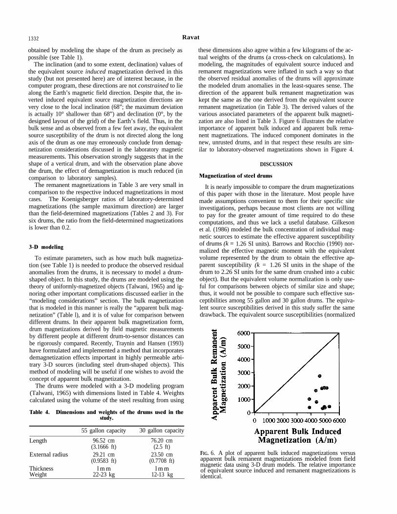
these dimensions also agree within a few kilograms of the ac-tual weights of the drums (a cross-check on calculations). Inmodeling, the magnitudes of equivalent source induced andremanent magnetizations were inflated in such a way so thatthe observed residual anomalies of the drums will approximatethe modeled drum anomalies in the least-squares sense. Thedirection of the apparent bulk remanent magnetization waskept the same as the one derived from the equivalent sourceremanent magnetization (in Table 3). The derived values of thevarious associated parameters of the apparent bulk magneti-zation are also listed in Table 3. Figure 6 illustrates the relativeimportance of apparent bulk induced and apparent bulk rema-nent magnetizations. The induced component dominates in thenew, unrusted drums, and in that respect these results are sim-ilar to laboratory-observed magnetizations shown in Figure 4.

DISCUSSION

Magnetization of steel drums

It is nearly impossible to compare the drum magnetizationsof this paper with those in the literature. Most people havemade assumptions convenient to them for their specific siteinvestigations, perhaps because most clients are not willingto pay for the greater amount of time required to do thesecomputations, and thus we lack a useful database. Gilkesonet al. (1986) modeled the bulk concentration of individual mag-netic sources to estimate the effective apparent susceptibilityof drums (k = 1.26 SI units). Barrows and Rocchio (1990) nor-malized the effective magnetic moment with the equivalentvolume represented by the drum to obtain the effective ap-parent susceptibility (k = 1.26 SI units in the shape of thedrum to 2.26 SI units for the same drum crushed into a cubicobject). But the equivalent volume normalization is only use-ful for comparisons between objects of similar size and shape;thus, it would not be possible to compare such effective sus-ceptibilities among 55 gallon and 30 gallon drums. The equiva-lent source susceptibilities derived in this study suffer the samedrawback. The equivalent source susceptibilities (normalized

FIG. 6. A plot of apparent bulk induced magnetizations versusapparent bulk remanent magnetizations modeled from fieldmagnetic data using 3-D drum models. The relative importanceof equivalent source induced and remanent magnetizations isidentical.

Magnetic Properties of Steel Drums 1333

to 1 cu ft volume) range from 45.90 to 51.66 SI units (3.65 to4.11 cgs units) for 55 gallon drums and from 21.50 to 28.77 SIunits (1.71 to 2.29 cgs units) for 30 gallon drums. The appar-ent bulk susceptibilities or the apparent bulk magnetizationsderived in this study (Table 3) are the closest things to “bulk”reality using the theory of uniformly magnetized objects as faras the steel drums are concerned. Breiner (1973) mentionedthat for most iron and steel objects the susceptibility is be-tween and 125 (SI units) or 1 and 10 (cgs units), and theapparent bulk susceptibilities derived here are in agreementwith his values. However, modeling in the shape of the drums(including the magnetization-wise empty space) is necessaryto derive these values; the other important drawback is theamount of time required to specify precisely the 3-D shape ofthe object—a very difficult task if the drums were tilted.

Viscous magnetization is a complicating factor that is notconsidered here at great length because of lack of constrain-ing information. Although viscous effects in steel drums arenot studied extensively, a preliminary study in Gilkeson et al.(1992) suggests that they can be large (a few tens of nT)over the time span of just a few hours. This effect will bepresent in the apparent magnetic susceptibilities and magne-tizations derived from field-magnetic measurements (see also,Macnae, 1994), but probably not the laboratory measurementsof the susceptibility. Because different drum orientations hadto be used in this study to derive the induced and remanent

magnetizations from the field-magnetic measurements, the vis-cous effects probably contribute toward both induced and re-manent magnetizations (but their respective amounts cannotbe quantified).

Neither any field-derived remanent magnetization data onsteel drums nor any laboratory magnetization data on samplesfrom steel drums are known to the author. It is, however, in-teresting to note that the laboratory-derived susceptibilities inthe maximum direction and the potential susceptibilities givenin Table 2 are within the range specified in Breiner (1973) andthe apparent bulk susceptibilities derived in this study. The ap-parent bulk remanent magnetizations, on the other hand, arehigher than the laboratory-derived remanent magnetizations(but certainly within an order of magnitude).

Modeling efficiency

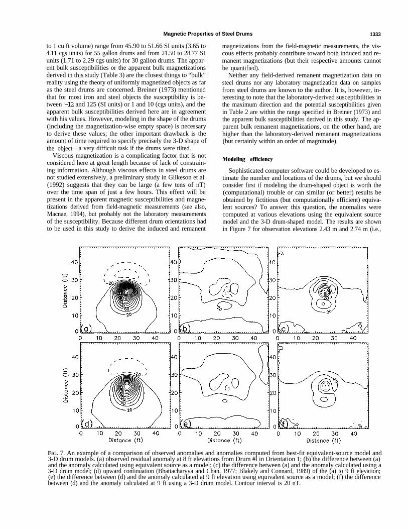
Sophisticated computer software could be developed to es-timate the number and locations of the drums, but we shouldconsider first if modeling the drum-shaped object is worth the(computational) trouble or can similar (or better) results beobtained by fictitious (but computationally efficient) equiva-lent sources? To answer this question, the anomalies werecomputed at various elevations using the equivalent sourcemodel and the 3-D drum-shaped model. The results are shownin Figure 7 for observation elevations 2.43 m and 2.74 m (i.e.,

FIG. 7. An example of a comparison of observed anomalies and anomalies computed from best-fit equivalent-source model and3-D drum models. (a) observed residual anomaly at 8 ft elevations from Drum #l in Orientation 1; (b) the difference between (a)and the anomaly calculated using equivalent source as a model; (c) the difference between (a) and the anomaly calculated using a3-D drum model; (d) upward continuation (Bhattacharyya and Chan, 1977; Blakely and Connard, 1989) of the (a) to 9 ft elevation;(e) the difference between (d) and the anomaly calculated at 9 ft elevation using equivalent source as a model; (f) the differencebetween (d) and the anomaly calculated at 9 ft using a 3-D drum model. Contour interval is 20 nT.

1334

1.47 m and 1.78 m above the top of the drums, respectively).These results strongly indicate that the equivalent sourcemodel better represents the observed and upward-continuedanomaly fields at these source-to-observation distances (interms of anomaly fall-off rate, amplitude, and shape of theanomaly) than the 3-D drum-shaped model itself. Above theseobservation elevations (with the drum placed vertically on theground surface), both models work equally well. The differ-ence between the observed anomaly and the anomaly com-puted from the 3-D drum-shaped models (Figures 7c and 7f)may be caused by the nonuniformity of the magnetic fieldwithin the body (as discussed earlier). As far as the fit of theequivalent source model is concerned (Figures 7b and 7e), thevertical location of the equivalent source was determined basedon the fit of the calculated anomalies to observed anomalies(through Euler’s equation). It is therefore not surprising thatthe equivalent source model fits the observed anomalies bet-ter than the anomalies calculated from the 3-D drum-shapedobject. In any case, for the purpose of estimating the numberof buried drums, the results in Figure 7 fail to show any com-pelling reason to adhere to the 3-D drum-shaped model-theequivalent source model fits the anomaly better and is compu-tationally most efficient. The equivalent source magnetizationsderived in this study should be of value in estimating the num-ber and locations of the drums. The problem can be handledwith iterative forward modeling using equivalent sources andthe ranges of equivalent source susceptibilities and remanentmagnetizations derived in this paper.

Changes in magnetic anomalies caused by rusting

Although this paper is not about rusted drums, some discus-sion on the effects of rusting would be appropriate. The drumsused in this study are being rusted naturally in the air (in Ori-entation 1) and the changing magnetic anomalies are beingmonitored every six months. The initial changes in magneticanomalies caused by oxidation appear to be complex in detail.Magnetic anomalies of some drums decreased systematicallywith increasing oxidation, in others the changes are within theerror level, and in yet another group of drums, the anomaliesappeared to increase slightly and then started falling-off withincreasing oxidation. At the present time, rusting has not pen-etrated much beneath the surface of the drums. Based on thepresent data, one cannot confirm or refute the hypothesis thatthe process of rusting alone will significantly reduce the mag-netic properties of steel drums. It seems likely, however, thatthe reduction may be achieved if the rust is physically removedfrom the drums (and thereby reducing the available magneticmaterial).

CONCLUSION

The results of the study are:

1) Laboratory-measured magnetizations are smaller thanthe magnetizations needed to model 55 and 30 gallon steeldrums (e.g., compare susceptibilities and remanent mag-netization values in Table 2 and apparent bulk suscepti-bilities and remanent magnetization values in Table 3).The comparisons indicate that if the laboratory magneti-zation values were used to model steel drums, the calcu-lated magnetic anomalies would significantly fall short ofthe observed magnetic anomalies;

Ravat

2)

3)

4)

5)

In the new (unrusted) drums, the induced componentis much larger than the remanent component based onlaboratory- and field-derived magnetizations;The equivalent source magnetization ranges for verticaldrums are: (a) 55 gallon drums-Volume susceptibi-lity-45.90 to 51.66 SI units (3.65 to 4.11 cgs units), manent magnetization-140 to 1200 A/m (0.14 to 1.20emu/cm3); (b) 30 gallon drums—Volume susceptibility—21.50 to 28.77 SI units (1.71 to 2.29 cgs units), Remanentmagnetization-98 to 410 A/m (0.09 to 0.41 emu/cm3)(the values are normalized to 1 cu ft volume and whenequivalent source is placed 0.5 ft above the bottom centerof the drum and based on only eight 55 gallon and four30 gallon drums);The apparent bulk magnetization ranges are (based ontwelve drums): Volume susceptibility- to SI units to cgs units), and Remanent magnetiza-t i o n - to A/m (-0.325 to andThe equivalent source model, placed at an optimum lo-cation, better approximates the observed anomalies thanthe 3-D modeling of the drums at most practical source-to-observation distances encountered in environmentalinvestigations.

ACKNOWLEDGMENTS

would like to thank Rick Blakely, Bill Hinze, and BruceMoskowitz and the three reviewers and the Associate Editorof GEOPHYSICS for their careful comments on the manuscript.The research was supported by Special Research Project ofthe Office of Research, Development, and Administration ofSouthern Illinois University at Carbondale. Dean AnthonyYoung of the College of Agriculture made available the sitefor the field surveys. Steve Stubblefield and Elden Chaffnerprovided considerable logistical help for the Drums Project.The field magnetic measurements were made by MechelleCrisler and Coulibaly Mammadou. Bruce Moskowitz, PaulKelso, Chris Hunt, and Jim Marvin of the Institute of RockMagnetism, University of Minnesota, provided considerablehelp and advice in making laboratory magnetic measurements.Linda Gassel retyped the unrecovered parts of the manuscriptand tables in the matter of hours after the crash of my harddrive. I am grateful for the generous help of all of theseindividuals and organizations.

REFERENCES

Barrows, L., and Rocchio, J. E., 1990, Magnetic surveying for buriedmetallic objects: Ground Water Monitoring Review, 10, 204-211.

Bhattacharyya, B. K., and Chan, K. C., 1977, Reduction of magneticand gravity data on an arbitrary surface acquired in a region of hightopographic relief: Geophysics, 42, 1411-1430.

Blakely, R. J., 1995, Potential theory in gravity and magnetic applica-tions: Cambridge Univ. Press.

Blakely, R. J., and Connard, G. C., 1989, Crustal studies using magneticdata, in Mooney, W. D., and Pakiser, L. C., Eds., Geophysical frame-work of the continental United States: Geol. Soc. Am. Memoir, 172,45-60.

Breiner, S., 1973, Applications manual for portable magnetometers:GeoMetrics.

Dampney, C. N. G., 1969, The equivalent source technique: Geo-physics, 34, 39-53.

Gilkeson, R. H., Heigold, P. C., and Laymon, D. E., 1986, Practicalapplication of theoretical models to magnetometer surveys on haz-ardous waste disposal sites—A case history: Ground water moni-toring review, 6, 54-61.

Magnetic Properties of Steel Drums 1335

Gilkeson, R. H., Gorin, S. R., and Laymon, D. E., 1992, Application ofmagnetic and electromagnetic methods to metal detection, in Bell,R. S., Ed., Proc. Symp. on the application of geophysics to engineer-ing and environmental problems, Vol. 1: Soc. Eng. and Min. Expl:Geophys., 309-328.

Grant, F. S., and West, G. F., 1965, Interpretation theory in appliedgeophysics: McGraw-Hill Book Co.

Hinze, W. J., 1990, The role of gravity and magnetic methods inengineering and environmental applications, in Ward, S. H., Ed.,Geotechnical and Environmental Geophysics, Vol. 1: Soc. Expl.Geophys., 75-126.

Macnae, J., 1994, Viscous magnetization: Misleading Koenigsberger’sQ: 64th Ann. Internat. Mtg., Soc. Expl. Geophys., Expanded Ab-stracts, 456-458.

McKeehan, L. W., 1967, Magnets: D.Van Nostrand Co.Ravat, D., 1994, Use of the fractal dimension to determine the applica-

bility of Euler’s homogeneity equation for finding source locationsof gravity and magnetic anomalies, in Bell, R. S., and Lepper, C. M.,Eds., Proc. Symp. on the application of geophysics to engineering

and environmental problems, Vol. 1: Environ. and Eng. Geophys.Soc, 41-53.

Skilbrei, J. R., 1993, The straight-slope method for basement depthdetermination revisited: Geophysics, 58, 593-595.

Talwani, M., 1965, Computation with the help of a digital computerof magnetic anomalies caused by bodies of arbitrary shape: Geo-physics, 30, 797-817.

Talwani, M., and Heirtzler, J. R., 1964, Computation of magneticanomalies caused by two dimensional structures of arbitrary shape:Computer in the mineral industries, Part 1, Stanford UniversityPubl., Geological Sciences, 9, 464-480.

Thompson, D. T., 1982, EULDPH-A new technique for makingcomputer-assisted depth estimates from magnetic data: Geophysics,47, 31-37.

Traynin, P., and Hansen, R. O., 1993, Magnetic modeling for highlypermeable bodies with remanent magnetization: 63th Ann. Internat.Mtg., Soc. Expl. Geophys., Expanded Abstracts, 410-413.

Westphalen, O., and Rice, J., 1992, Drum detection: EM versus Mag:Some revealing tests: Proc. 6th Nat. Outdoor Action Conf., 665-688.

View publication statsView publication stats