Embed Size (px)
Citation preview

Dipl.-Ing. Christoph Stefan Aigner
Magnetic resonance RF pulse design forsimultaneous multislice imaging
DOCTORAL THESIS
to achieve the university degree of
Doktor der technischen Wissenschaften
submitted to
Graz University of Technology
SupervisorUniv.-Prof. Dipl-Ing. Dr.techn. Rudolf Stollberger
Institute for Medical Engineering
Graz, 2018

Statutory Declaration
I declare that I have authored this thesis independently, that I have not used otherthan the declared sources/resources, and that I have explicitly marked all materialwhich has been quoted either literally or by content from the used sources.
Graz,
Date Signature
Eidesstattliche Erklarung1
Ich erklare an Eides statt, dass ich die vorliegende Arbeit selbststandig verfasst,andere als die angegebenen Quellen/Hilfsmittel nicht benutzt, und die den benutztenQuellen wortlich und inhaltlich entnommenen Stellen als solche kenntlich gemachthabe.
Graz, am
Datum Unterschrift
1Beschluss der Curricula-Kommission fur Bachelor-, Master- und Diplomstudien vom 10.11.2008;Genehmigung des Senates am 1.12.2008
ii

Acknowledgements
This work was carried out during the years 2012-2018 at the Graz University ofTechnology, at the Institute of Medical Engineering in strong and tight cooperationwith researchers from the Department of Mathematics at the Karl Franzens Universityof Graz. It is a pleasure to thank those who made this thesis possible.
Firstly, I would like to thank my supervisor Prof. Rudolf Stollberger for introducingme to the exciting research field of magnetic resonance imaging (MRI), his continuoussupport and optimism concerning this work and for giving me the opportunity towork on this topic. RF pulse design for MRI is a highly interdisciplinary research fieldthat requires knowledge from various topics including physics, computer science,engineering, medicine and mathematics. Therefore, I would like to point out thatthe working environment as a member of the SFB Research Center ”MathematicalOptimization and Applications in Biomedical Sciences” turned out to be optimal forthe progress of this thesis. Hence, a special thanks goes to Prof. Karl Kunisch as theCoordinator of the SFB for his support and cooperation. In addition, I would like tohighlight two people, Prof. Christian Clason and Armin Rund. You have been mytwo main collaborators and I owe you my deepest gratitude for your endless patience,support and motivating guidance. Moreover, the results presented in this work wereonly possible thanks to our tight and fruitful cooperation. Thank you! I am lookingforward to further joint work in the future.
Further, I want to express my immense gratitude to all present and former colleaguesat the Institute of Medical Engineering (TU Graz), the Institute of Mathematics and Sci-entific Computing (Uni Graz), the Institute of Psychology (Uni Graz), the Departmentof Neurology (Medical University) and the Ludwig Boltzmann Institute for ClinicalForensic Imaging for numerous interesting and highly productive discussions and therelaxed working atmosphere. Special thanks go to Deepika Bagga, Christoph Birkl,Markus Bodenler, Prof. Kristian Bredies, Clemens Diwoky, Christian Gossweiner,Christina Graf, Kamil Kazimierski, Karl Koschutnig, Markus Kraiger, ChristianLangkammer, Andreas Lesch, Oliver Maier, Adrian Martın Fernandez,BernhardNeumayer, Peter Opriessnig, Isabella Radl, Lukas Pirpamer, Prof. Stefan Ropele,Andreas Petrovic, Prof. Veronika Schopf, Prof. Hermann Scharfetter, MatthiasSchlogl, Martin Sollradl, Johannes Strasser, Stefan Spann and Bridgette Webb.
iii

I am thankful for the great time we had together and I am glad I got to share the lastyears with you.
I would additionally like to thank my so far not mentioned national and internationalcooperation partners from the Medical University of Vienna, King’s College Londonand the MGH Harvard-MIT group in Boston, especially, Samy Abo Seada, Prof.Elmar Laistler, Prof. Shaihan Malik, Lena Nohava, Prof. Gert Pfurtscheller, DanielPolak and Prof. Kawin Setsompop. The collaboration with you has allowed me toextend and deepen my knowledge of various exciting MR related topics previouslyunknown to me. Thank you!
Very special thanks go to all proofreaders, especially A. Lesch and B. Webb, whosecomments greatly helped me to polish and to finish this thesis.
I extend my deepest gratitude to my friends and everyone else who is not listed hereexplicitly. Finally, I would like to thank my girlfriend Sara, my brother Michael andmy parents Stefan and Gertraud Aigner for their continuous love, help and endlesssupport. This journey would not have been possible without you!
iv

Abstract
Magnetic Resonance Imaging (MRI) is one of the leading non-invasive medicalimaging techniques to image healthy and pathological anatomy and physiologicalprocesses of the body and is primarily known for its excellent soft tissue contrast.Contrary to other high resolution imaging techniques, MRI is based on strong mag-netic and electric fields and does not require ionizing radiation. Image acquisition,however, is often limited by long acquisition times resulting from the need to repeatthe measurement several times to encode multiple k-space data points. In addition tolengthy acquisition times, limited MR hardware performance as well as physical andphysiological effects further restrict the MR sequence parameters, which results inlower signal to noise ratio and increased sensitivity to motion or magnetic susceptibil-ity effects. This thesis is dedicated to the development and practical implementationof tailored large tip-angle radio frequency (RF) pulses and slice selective gradientshapes with increased excitation accuracy, lower power requirement and reducedpulse duration. The presented optimal control based RF pulse design methods areformulated for the joint design of RF and slice selective gradient shape for differentlarge tip-angle applications. The focus of this work is on simultaneous multislice(SMS) applications to push acceleration of existing 2D MRI acquisition strategies. Theextension to constrained RF pulse optimization allows exploitation of various MRhardware limits and yields accurate low power RF pulses and slice selective gradientshapes with short pulse durations. The optimized waveforms proved to outperformexisting RF pulses and can be used to reduce the minimal echo spacing and echo time.Numerous simulation and experimental examples based on phantom and in-vivomeasurements demonstrate the increased excitation accuracy and the reduction ofboth RF power and RF duration.
Keywords: RF pulse design, slice-selective, simultaneous multislice, refocusing, phys-ical constraints, optimal control
v
Kurzfassung
Die Magnetresonanztomographie (MRT) ist eines der fuhrenden nicht-invasivenbildgebenden Verfahren zur Abbildung gesunder und pathologischer Gewebstypenund physiologischer Prozesse des Korpers und ist vor allem fur seinen hervor-ragenden Weichteilkontrast bekannt. Im Gegensatz zu anderen hochauflosendenbildgebenden Verfahren basiert die MRT auf starken magnetischen und elektrischenFeldern und benotigt keine schadliche ionisierende Strahlung oder Rontgenstrahlung.Die Bildaufnahme ist jedoch oft durch lange Aufnahmezeiten begrenzt, die sich ausder Notwendigkeit ergeben, die Messung mehrmals zu wiederholen, um mehrerek-space Datenpunkte zu kodieren. Zusatzlich zu den langen Messzeiten, begrenzendie limitierte MR-Hardware und physische und physiologische Beschrankungendie MRT Sequenzparameter, was zu einem geringeren Signal-Rausch-Verhaltnisund einer hoheren Empfindlichkeit fur Bewegungseffekte fuhrt. Diese Arbeit wid-met sich der Entwicklung und praktischen Umsetzung maßgeschneiderter Hochfre-quenzpulse und schichtselektiver Gradientenformen mit erhohter Anregungsge-nauigkeit, geringem Leistungsbedarf und reduzierter Pulsdauer. Die vorgestelltenHF-Impulsentwurfsmethoden basieren auf Methoden der Optimalsteuerung und sindfur den gemeinsamen Entwurf von HF Puls und schichtselektiven Gradientenformformuliert. Der Schwerpunkt dieser Arbeit liegt auf der simultanen Mehrschich-tanwendungen zur weiteren Beschleunigung von 2D-MRT-Aufnahmestrategien. DieErweiterung der Designmethode auf die eingeschrankte Optimierung ermoglicht dieAusnutzung verschiedener MR-Hardware-Grenzen, was zu einer geringen Pulsleis-tung oder minimalen Dauer von HF-Impulsen und schichtselektiver Gradientenfor-men fuhrt. Die optimierten Wellenformen ubertreffen vorhandene HF-Impulse undkonnen dazu verwendet werden, das minimalen Echo-Spacing zu reduzieren unddie kurzeste erreichbare Echozeit zu nutzen. Zahlreiche Simulations- und Experimen-talbeispiele auf Basis von Phantom- und In-vivo-Messungen zeigen die Erhohungder Anregungsgenauigkeit, die Reduzierung der HF-Leistung und die Reduktion derminimalen HF-Dauer.
Schlusselworter: Magnetresonanztomographie, HF-Impulsdesign, schichtselektiv,Simultane Multischicht-Anregung, Refokussierung, optimale Steuerung
vi
Contents
Abstract v
Acronyms ix
1 Introduction 1
2 Physical principles of magnetic resonance 32.1 Nuclear spin . . . . . . . . . . . . . . . . . . . . . . . . . . . . . . . . . . 4
2.2 Equation of motion and bulk magnetization . . . . . . . . . . . . . . . 6
2.3 RF excitation . . . . . . . . . . . . . . . . . . . . . . . . . . . . . . . . . . 9
2.4 Relaxation . . . . . . . . . . . . . . . . . . . . . . . . . . . . . . . . . . . 11
2.5 Bloch equations . . . . . . . . . . . . . . . . . . . . . . . . . . . . . . . . 13
3 Bloch simulation 163.1 Neglected relaxation . . . . . . . . . . . . . . . . . . . . . . . . . . . . . 17
3.1.1 Small tip angle approximation . . . . . . . . . . . . . . . . . . . 17
3.1.2 Rotation in the magnetization domain . . . . . . . . . . . . . . . 18
3.1.3 Rotation in the spin domain . . . . . . . . . . . . . . . . . . . . 21
3.2 Including relaxation . . . . . . . . . . . . . . . . . . . . . . . . . . . . . 23
4 MR hardware and practical aspects 264.1 Experimental design . . . . . . . . . . . . . . . . . . . . . . . . . . . . . 27
4.2 Pulse sequence programming . . . . . . . . . . . . . . . . . . . . . . . . 31
4.3 RF pulse and slice selective gradient limitations . . . . . . . . . . . . . 32
5 RF pulse design 385.1 RF pulse categories . . . . . . . . . . . . . . . . . . . . . . . . . . . . . . 39
5.2 Spatial non-selective RF pulses . . . . . . . . . . . . . . . . . . . . . . . 41
5.3 Spatial selective RF pulses . . . . . . . . . . . . . . . . . . . . . . . . . . 44
5.4 Variable-rate selective excitation . . . . . . . . . . . . . . . . . . . . . . 51
5.5 SMS RF pulse design . . . . . . . . . . . . . . . . . . . . . . . . . . . . . 52
5.5.1 Peak RF amplitude reduction . . . . . . . . . . . . . . . . . . . . 53
5.5.2 Peak RF amplitude and RF power reduction . . . . . . . . . . . 56
vii

Contents
5.6 Slice selective RF pulse design via optimal control . . . . . . . . . . . . 59
5.6.1 Single slice selective RF pulse design via OC . . . . . . . . . . . 60
5.6.2 SMS RF pulse design via OC . . . . . . . . . . . . . . . . . . . . 68
6 Discussion 81
7 Outlook 84
8 List of Publications 87
9 Appendix 939.1 Efficient high-resolution RF pulse design applied to simultaneous
multi-slice excitation . . . . . . . . . . . . . . . . . . . . . . . . . . . . . 93
9.1.1 Introduction . . . . . . . . . . . . . . . . . . . . . . . . . . . . . . 94
9.1.2 Theory . . . . . . . . . . . . . . . . . . . . . . . . . . . . . . . . . 96
9.1.3 Methods . . . . . . . . . . . . . . . . . . . . . . . . . . . . . . . . 100
9.1.4 Results . . . . . . . . . . . . . . . . . . . . . . . . . . . . . . . . . 104
9.1.5 Discussion . . . . . . . . . . . . . . . . . . . . . . . . . . . . . . . 110
9.1.6 Conclusions . . . . . . . . . . . . . . . . . . . . . . . . . . . . . . 113
9.1.7 Trust-region algorithm . . . . . . . . . . . . . . . . . . . . . . . . 114
9.1.8 Discretization . . . . . . . . . . . . . . . . . . . . . . . . . . . . . 115
9.2 Magnetic Resonance RF pulse design by optimal control with physicalconstraints . . . . . . . . . . . . . . . . . . . . . . . . . . . . . . . . . . . 117
9.2.1 Introduction . . . . . . . . . . . . . . . . . . . . . . . . . . . . . . 118
9.2.2 Theory . . . . . . . . . . . . . . . . . . . . . . . . . . . . . . . . . 119
9.2.3 Methods . . . . . . . . . . . . . . . . . . . . . . . . . . . . . . . . 123
9.2.4 Results . . . . . . . . . . . . . . . . . . . . . . . . . . . . . . . . . 125
9.2.5 Discussion . . . . . . . . . . . . . . . . . . . . . . . . . . . . . . . 134
9.2.6 Conclusions . . . . . . . . . . . . . . . . . . . . . . . . . . . . . . 141
9.2.7 Lagrange calculus in the spin domain . . . . . . . . . . . . . . . 141
9.3 Simultaneous Multislice Refocusing via Time Optimal Control . . . . 145
9.3.1 Introduction . . . . . . . . . . . . . . . . . . . . . . . . . . . . . . 146
9.3.2 Theory . . . . . . . . . . . . . . . . . . . . . . . . . . . . . . . . . 147
9.3.3 Methods . . . . . . . . . . . . . . . . . . . . . . . . . . . . . . . . 151
9.3.4 Results . . . . . . . . . . . . . . . . . . . . . . . . . . . . . . . . . 155
9.3.5 Discussion . . . . . . . . . . . . . . . . . . . . . . . . . . . . . . . 161
9.3.6 Conclusions . . . . . . . . . . . . . . . . . . . . . . . . . . . . . . 164
Bibliography 169
viii

Acronyms
BIR B1 Insensitive RotationCAIPIRINHA Controlled Aliasing in Parallel Imaging Results in Higher Accelera-
tionCG Conjugate GradientCPMG Carr-Purcell-Meiboom-GillCPU Central Processing UnitCSPAMM Complementary Spatial Modulation of MagnetizationEPI Echo-planar imagingFFT Fast Fourier TransformFID Free Induction DecayFLASH Fast Low Angle Single ShotFOV Field-of-ViewFWHM Full Width at Half MaximumGIRF Gradient Impulse Response FunctionGPU Graphics Processing UnitGRAPPA Generalized Autocalibrating Partially Parallel AcquisitionsGRASE Gradient-and Spin-EchoGRE Gradient Recalled EchoIDEA Integrated Development Enviroment for (MR) ApplicationsISMRM International Society for Magnetic Resonance in MedicineMB MultibandMR Magnetic ResonanceMRI Magnetic Resonance ImagingNMR Nuclear Magnetic ResonanceOC Optimal ControlPINS Power Independent Number Of SlicespTx Parallel ExcitationRARE Rapid Acquisition with Refocused EchoesRF Radio FrequencyROI Region of Interest
ix

Acronyms
SAR Specific Absorption RateSE Spin EchosG slice GRAPPASINC Sinus CardinalisSLR Shinnar–Le RouxSMS Simultaneous Multi-SliceSPAMM Spatial Modulation of MagnetizationSSFP Steady-State Free PrecessionTBWP Time-Bandwidth ProductTE Echo TimeTHK ThicknessTR Repetition TimeTSE Turbo Spin EchoVERSE Variable-Rate Selective Excitation
x

1 Introduction
Most NMR and MR applications need RF pulses to alter magnetization and to createNMR signals, which makes them an essential element in MRI. RF pulses are eitherused without a slice selective gradient shape for spatial non-selective applications orsimultaneously with a slice selective gradient for slice selective excitation, inversionor refocusing and are an essential element of MRI sequences. Contrary to the staticmain field, RF and slice selective gradient fields are not applied continuously, butin distinct blocks or periods of MRI sequences with a time varying waveform. Yet,achieving well defined spatially selective slice profiles at high field strengths whilefulfilling hardware and safety constraints is a challenging task. Consequently, differ-ent design approaches were proposed for RF pulse design using different kind ofapproximations on the Bloch equations for various applications. These assumptions,for instance neglected relaxation terms or the small tip angle approximation, resultin analytical expressions with easy solutions and therefore find widespread use.However, the accuracy of conventional RF pulses is limited by the impact of theunderlying approximations. An alternative design approach is the minimization ofa suitable functional that represents a comprehensive description of the intendedRF pulse application. Different optimization methods have been proposed to solvethe design task including simulated annealing, evolutionary approaches or optimalcontrol. These design methods often lead to more accurate excitation patterns andallow to consider various other effects, for instance spatially varying slice selectivegradients or transmit coil sensitivities. However, the use of numerical optimizationtechniques are often limited by the computational effort. The main research questionthat forms the basis of this thesis consists in how numerical optimization can beused to jointly design RF pulse and slice selective gradient shapes for large flip angleapplications. Besides single slice selective excitation, the focus of this work lies onSMS applications. Different RF pulse design methods and models based on OC arediscussed. These include unconstrained and constrained optimization with fixed andvariable pulse duration [1]–[3]. The proposed optimization methods significantlyreduce the pulse duration with minimal RF power compared to state of the artRF pulse design methods [4]. Additionally to low RF power and pulse durationrequirements, the optimized results fulfil specific hardware and safety limitations.The system limitations can be defined before the optimization and include RF, sliceselective gradient and slew rate amplitude and RF power constraints and constraints
1

1 Introduction
on the slice profile accuracy. The optimized RF pulses are experimentally validatedand the applicability of the proposed design methods is proved.
The structure of this thesis is as follows. Chapter 2 revises the physical principlesof NMR and MR necessary to understand the specifications regarding the RF pulsedesign process and its substantial consequences. It contains a brief derivation of theBloch equations and description of MRI strategies for signal generation. Further, itdiscusses why the Bloch equations can be solved analytically only for special cases.The general simulation and solution of the Bloch equations is covered by Chapter 3.Different numerical and analytical Bloch integration methods, including rotationmatrices for piecewise constant fields, small tip angle approximation and analyticaleigenvalue approach are discussed and introduced. Chapter 4 summarizes specificaspects on the practical MR sequence implementation and hardware limitations. Thefocus of this chapter lies in the practical validation of the optimized RF pulse and sliceselective gradient waveforms and the impact of hardware limits and imperfections.The design of RF pulses is covered by Chapter 5. This chapter discusses the mostprominent RF pulse design methods for single non- and slice selective and SMSselective excitation and refocusing. The main results of the three main publicationsof this thesis [1]–[3] are summarized at the end of Chapter 5 and are listed in theAppendix. The final discussion and outlook for further applications on the design ofparallel transmission and the inclusion of gradient imperfections in the optimizationare given in Chapters 6 and 7.
2

2 Physical principles of magneticresonance
Contents
2.1 Nuclear spin . . . . . . . . . . . . . . . . . . . . . . . . . . . . . . 4
2.2 Equation of motion and bulk magnetization . . . . . . . . . . . . 6
2.3 RF excitation . . . . . . . . . . . . . . . . . . . . . . . . . . . . . . 9
2.4 Relaxation . . . . . . . . . . . . . . . . . . . . . . . . . . . . . . . 11
2.5 Bloch equations . . . . . . . . . . . . . . . . . . . . . . . . . . . . 13
Nuclear magnetic resonance (NMR) or more general, magnetic resonance (MR)is based on the quantum mechanical interaction of atomic nuclei with a nonzeronuclear magnetic moment and an external magnetic field B0 [5]–[8]. Besides NMRapplications in the field of material research or chemical analysis, the NMR effectcan further be used to perform magnetic resonance imaging (MRI) to acquire non-invasive images with excellent soft-tissue contrast. The quantum mechanical effects ofindividual spins can be summarized for a sample with a large number of spins by aclassical description of the macroscopic bulk magnetization [7], [8] whose interactionswith the external magnetic field can be modeled by the classical phenomenologicalBloch equations [9]. Although this macroscopic description does not include nuclearspin-spin interactions such as j-, dipole-, or quadrupole-coupling, it is sufficient tomodel the most effects for the intended clinical in vivo MRI applications to imagethe hydrogen proton. Therefore, the quantum mechanical content in this section isreduced to an absolute minimum. For a quantum mechanical description of NMRthe reader is refered to [8], [10] and for an analysis of different MRI myths caused byan incorrect interpretation of quantum mechanics to [11].
In the following section, the emphasis will be on the classical description of the mag-netization regarding the effects of an external field on non-zero spins. Furthermore,all discussion is limited to hydrogen protons.
3

2 Physical principles of magnetic resonance
2.1 Nuclear spin
The observations of Zeeman [12], Stern and Gerlach [13], Uhlenbeck and Goudsmith[14] and Dirac [15] led to the introduction of the electron spin and the observation,that the quantum mechanical states of atoms in a constant external magnetic fieldsplit into discrete energy levels. Figure 2.1 shows such a schematic energy splittingof the proton in an external magnetic field. The energy difference E∆ is generallydefined by the Zeeman Hamiltonian
Hz = −γhB0 Iz, (2.1)
using the quantum mechanical spin operator Iz, the reduced Planck constant h =1.0545718 · 10−34 J s [16], the gyromagnetic ratio γ in rad s−1 T−1 and the main fieldB0 in T. For the hydrogen proton with a nuclear spin I = 1/2 the magnetic spinquantum number
ms = −I, (−I + 1), (−I + 2), ..., I (2.2)
results in ms = ±1/2. The two energy levels of the eigenstates can be found usingthe Schrodinger equation
Hz|I, ms >= E|I, ms >, (2.3)
with the energy E and eigenfunction of the proton |I, ms >. Using Eq. 2.1 and 2.2 theenergy difference E∆ or transition between the two states can be computed with
E∆ = 1/2γhB0 − (−1/2γhB0) = hω0, (2.4)
describing the static interaction with the external magnetic field B0.
This expression directly leads to the Lamor equation
ω0 = −γB0, (2.5)
with the nuclei dependent proportionality factor or gyromagnetic ratio γ given by
γ =gpµn
h, (2.6)
with the experimentally determined proton Lande-factor gp = 5.58 [17] and thenuclear magnetic moment µn. The nuclear magnetic moment is defined as
µn =eh
2mp, (2.7)
4

2 Physical principles of magnetic resonance
with the magnitude of the particle charge e = 1.60 × 10⁻¹⁹ C and the protonmass mp = 1.67 × 10⁻²⁷ kg, see [8]. For protons, γ is 2.6731 × 10⁸ rad s−1 T−1 orγ/2π = 42.58 MHz/T [8]. The proton’s energy difference E∆ for the two stableenergy levels then mainly depends on the field strength, see Eq. 2.1. For a static fieldof B0 = 3 T this energy difference is E∆ = 8.457 × 10⁻²⁶ J.
The population ratio of the atoms occupying the two different states is described bythe Boltzmann distribution
E[N1]
E[N2]= e
E∆kT , (2.8)
using the reduced Boltzmann constant k = 1.381 × 10⁻²³ J K−1, the temperature Tin K and the energy difference E∆ to predict the different spin populations E[N1]and E[N2]. From that, one can calculate the macroscopic net magnetization that isproportional to the occupancy difference
E[N1 − N2] = Ne
E∆kT − 1
eE∆kT + 1
≈ NE∆
2kT, (2.9)
with N being the total number of spins [18]. At a field strength of 3 T and at roomtemperature T = 293.15 K the occupation difference is approximately 10 ppm.
Energy
0
no field external field
m=-1/2
m=1/2E1
E2
ΔE=E2-E1
Figure 2.1: Schematic Zeeman splitting of the proton energy levels in an external field. The Energydifference E∆ depends mainly on the external field, see Eq. 2.4.
Due to its high natural abundance in biological tissue and its large gyromagneticratio, hydrogen protons are the nuclei primarily used for in vivo MRI. Nevertheless,other nuclei with a non-zero spin, for instance 13C, 19P or 31P, also have a nuclearmagnetic moment µn that can be used to generate NMR signals. The nuclear magneticmoment µn can be related to the angular momentum J (the hats above the symbolindicate that they are quantum mechanical operators, refer to Chapter 7 of [10])
µn = γ J, (2.10)
5

2 Physical principles of magnetic resonance
with J = ( Jx, Jy, Jz)T in the Cartesian coordinates. For a quantum mechanical descrip-tion of the spin precession refer to Chapter 10 of [10].
The placement of a spin in an external magnetic field B results in a torque N =(Nx, Ny, Nz)T, given by the cross product of the magnetic spin moment µn and theexternal field B
N = µn × B. (2.11)
For a non-zero net torque this implies that the angular momentum J changes accord-ing to
dJdt
= N, (2.12)
establishing the fundamentals of the equation of motion. For a more rigorous deriva-tion of the magnetic moment and net force, referred to Chapter 2 of [8] and Chapters2 and 5 of [10].
2.2 Equation of motion and bulk magnetization
Combining Eq. 2.10 and Eq. 2.11 allows rewriting of Eq. 2.12 to get the fundamentalequation of motion:
dµn
dt= γµn × B. (2.13)
This differential equation describes the macroscopic movement of the spin momentin an external field B and relates the resulting motion to the gyromagnetic ratio γ[8]. For a static and time invariant external field, for instance B = (0, 0, B0)
T, Eq. 2.13
reduces to the important Lamor equation, see also Eq. 2.5, with ω0 describing theprecessional frequency of the spin system, better known as Lamor or precessionfrequency [8], [10]. The negative sign of Eq. 2.5 results from the main field B0 pointingalong the positive z-axis.
Pure water has a proton concentration of 110.4 mol L−1 [19], thus resulting in anextremely large number of protons for typical NMR or MRI sample sizes. Thisholds for most biological tissues, for instance grey matter of the brain has a protonconcentration of approximately 70 % of pure water [19]. For such a large number ofindividual protons, the macroscopic bulk magnetization M can be defined as the sumof all nuclear spins µn in the observed sample
M =1V ∑
protonsinVµn. (2.14)
6

2 Physical principles of magnetic resonance
dx
dy
dz
M0
B0
Figure 2.2: Random spin orientation and schematic build up of the makroscoptic bulk magnetizationin an external field B0.
with the volume V. In the absence of an external field, the direction of the individualspins is purely random due to random thermal motion [8], [10], thus resulting in noobservable bulk magnetization M = (0, 0, 0)T. However, immediately after applyinga strong external magnetic field, a precession around the external magnetic field istriggered. The random spin orientation (spherical) is slightly skewed towards the fielddirection due to relaxation [11] and a macroscopic observable bulk magnetizationaccumulates. The macroscopic bulk magnetization M now describes the macroscopicbehaviour in the external field and enables the use of classical descriptions ratherthan requiring quantum mechanics. Figure 2.2 shows the schematic build up of theclassical bulk magnetization M0 parallel to an external field.
Further, the assumption of non-interacting spins (for coupled spins, refer to Chapter 6
of [10]) and the previously defined bulk magnetization (Eq. 2.14) allow substitution ofthe magnetic moment µn in the equation of motion (Eq. 2.13) leading to a predecessorof the Bloch equations without relaxation effects
dM(t)dt
= γM(t)× B(t),
M(0) = M0,(2.15)
with the initial magnetization
M0 = [M0x, M0
y, M0z ]
T. (2.16)
Now, the change of magnetization M over time can be formulated as a result of theexternal magnetic field B on the magnetization M. The magnitude of the macroscopicbulk magnetization M0 scales for a hydrogen proton in the equilibrium (t→ inf)
M0 'γ2h2B0
4kTsampleρ0, (2.17)
7

2 Physical principles of magnetic resonance
with the magnitude of the applied field B0, Boltzmann’s constant k, reduced Plank’sconstant h, the sample temperature Tsample in K, the proton density ρ0 and the protonsgyromagnetic ratio γ according to [8].
This implies that in general, a stronger constant magnetic field results in a largerbulk magnetization and thus, a larger MR signal. However, increasing the mainfield strength causes several other effects which counteract this increase to someextent, for instance elevated B0 field inhomogeneities and an increased dielectriceffect. Furthermore, larger relaxation times and power deposition in combination withperipheral nerve stimulation, limit the optimal field strength for in vivo MR. Therefore,most clinical MR scanners nowadays still use 1.5 to 3 T [20], while human in vivo MRresearch is done up to 10.5 T [21]. The constant improvement of MR hardware andthe use of sophisticated MR techniques, recently resulted in the regulatory approvalof 7 T systems to be used for clinical routine applications [22]. For more informationon the impact of the hardware the reader is referred to Chapter 4.
The equation of motion Eq. 2.15 is defined with respect to a stationary coordinatesystem, better known in NMR as the laboratory frame of reference [8]. Typically, theconstant main magnetic field (B0) is much larger than the radio frequency (RF) andgradient fields essential for MR signal generation and spatial MRI encoding. Thisresults in a clouding of the much smaller non-static field interactions by the constantLamor precession, see Figure 2.3 and requires a high temporal and spatial resolutionfor an accurate description of the magnetization. Furthermore, the bandwidth of RFand slice selective gradient waveforms are much lower than the Lamor frequency,see Section 4.3. This would result in an unjustifiably computational effort and thestatic field interaction is therefore typically removed by a coordinate transformationsimilar to a frequency demodulation in signal processing. The transformation of theCartesian coordinates (x, y, z) to the rotating frame of reference (x′, y′, z′) with ωby
x′ = x cos(ωt)− y sin(ωt),y′ = x sin(ωt) + y cos(ωt),z′ = z.
(2.18)
In the following, the prime character is used to define variables in the rotatingframe of reference. The use of a rotating frame of reference rotating with the Lamorfrequency allows for an easier handling of the equations (see Section 2.3) and a betterunderstanding of the non-static field interactions [8], [10], [23]. Figure 5.1 summarizesthe differences between the laboratory frame of reference and the rotating frame ofreference. Instead of modulation of the RF pulse with the Lamor frequency ω0, therotation of the coordinate system with ω0 results in a stationary and on-resonantB1 field for the rectangular envelope, while the magnitude varies to achieve a SINC
8

2 Physical principles of magnetic resonance
envelope. The use of the rotating frame of reference simplifies the modelling of RFexcitation and signal encoding.
2.3 RF excitation
The equilibrium bulk magnetization M, see Eq. 2.14, does not result in a measurableMR signal [8], [10], [23]. To induce a NMR signal in nearby receiver coils, time varyingRF fields B1(t), for instance perpendicular to the much larger but constant field B0[8], are applied by setting
B(t, r) = [B1,x(t), B1,y(t), B0 + Gs(t) · r]T, (2.19)
with the slice selective gradient for each axis
Gs(t) = [Gs,x(t), Gs,y(t), Gs,z(t)]T, (2.20)
at spatial position r = (x, y, z)T being assumed to be zero for the discussion of pureRF excitation. RF fields close to or at the Lamor frequency tip the magnetization awayfrom the initial state M0, see Eq. 2.16. After the RF field is turned off, the transversalcomponents of the tipped magnetization precess around the B0 field with the Lamorfrequency Mxy(t) = (Mx(t), My(t))T and result in an electromagnetic induction inthe receiver coil [8], [10], see Figure 2.3 The time course of the magnetization M canbe modeled with Eq. 2.15.
While the general solution is hard to solve, see Section 3, the use of a left-circularpolarized RF field
B+1 (t) = B1
(cos ωt− sin ωt
), (2.21)
with B1 being the RF magnitude, ω the frequency and t the time vector allows findingof easy analytical solutions [8]. The further use of a rotating frame of reference [8],[24] rotating with the frequency ω instead of the laboratory frame of reference, resultsin a stationary RF field
B+1 (t)′ =
(B10
). (2.22)
9

2 Physical principles of magnetic resonance
The combination of B+1 (t)′ of Eq. 2.22 and Eq. 2.15, with a constant main field B0
according to [8], results in
(dM(t)
dt
)′= γM(t)′ ×
B10
B0 −ω/γ
= γM(t)′ × Be f f , (2.23)
with Be f f being the effective magnetic field and ω the frequency of the RF field. Thisresults in a counter clockwise precession around the axis of Be f f , see Figure 2.3. Forthe on-resonant case (ω = ω0) the B1 field is synchronized to tip the spin around thex′-axis and Eq. 2.23 is reduced to the cornerstone equation of motion
(dM(t)
dt
)′= γM(t)′ ×
B100
. (2.24)
Using Eq. 2.24 the overall rotation of the bulk magnetization can be described by theflip angle φ
φ = γ∫ T
t=0B1(t)dt, (2.25)
where T is the pulse duration and B1(t) is the time dependent RF modulationenvelope. For this easy example with an constant RF field B1, the flip angle φ can befurther analytically described by
φ = γB1T. (2.26)
However, it should be noted that Eq. 2.25 and 2.26 are valid only for the on-resonancecondition. A more comprehensive discussion of all factors influencing the flip angleand its measurment in MRI is given in [25].
So far, all considerations are mainly based on geometrical solutions resulting from theequation of motion (Eq. 2.15). An alternative solution to the RF excitation (Eq. 2.24)based on rotation matrices is described in Section 3. At this point it is importantto state again, that the simplified macroscopic view of the underlying quantummechanical spin properties is justified only for a large sample of non-interacting spins.For the quantum mechanical modelling of spins in external magnetic fields refer to[10].
10

2 Physical principles of magnetic resonance
B0
z
xy
M
B0
xy
Mxy
0
receivereceive
z
x'
y'
B1
M = 90°
(b)
(d)(c)
B0 B0
z
xy
M
B1
0
(a)
0
Figure 2.3: Schematic deflection of magnetization by a circular polarized RF field B1 in the laboratoryframe (a) + (b) and rotating frame of reference (d). After turning off B1, M precesses in thexy plane and induces a signal in the receive coil (c). Modified from [26].
2.4 Relaxation
Besides the interaction with external magnetic fields, there occur further spin inter-actions with each other and also with the surrounding. Since the exact quantummechanical mechanisms, which are responsible for these effects, are beyond thescope of this work, only the phenomenological observation of relaxation effects isdescribed here. For an extensive quantum mechanical explanation refer to [8], [10],[27], [28]. After tilting the bulk magnetization vector M by a RF pulse, it returnsback to its equilibrium state M = (0, 0, M0)
T after sufficient time. The macroscopiceffects behind this behaviour were modeled by Felix Bloch [9] as longitudinal (T1) andtransversal relaxation (T2) describing the time constants of a first order exponentialkinetics.
The longitudinal relaxation time T1 is defined as the proportionality factor that con-nects the recovery rate of the longitudinal magnetization (dMz/dt) and the differenceM0 −Mz
dMz(t)dt
=1T1
[M0 −Mz(t)],
Mz(0) = Mz0.
(2.27)
11

2 Physical principles of magnetic resonance
time in s
0 T1
2.5 5
Mz
0
1-e-1
M0
time in s
0 T2
0.25 0.5
Mxy
0
e-1
M0
Figure 2.4: Simulated recovery of the longitudinal (Mz) and transversal (Mxy) magnetization based onT1 and T2 relaxation for white matter at 3 T (T1 = 1084 ms, T2 = 69 ms, [29]).
This differential equation can be solved analytically yielding
Mz(t) = M0z e−t/T1 + M0(1− e−t/T1), (2.28)
with the initial condition M0z which describes the exponential recovery of the longitu-
dinal magnetization. Please note that the solution assumes that the external field B0is along the z-axis.
The transversal relaxation time T2 on the other hand is defined as the proportionalityfactor that connects the decay of the transversal magnetization (dMxy/dt)′ with theinitial condition M0
xy (
dMxy(t)dt
)′= − 1
T2Mxy(t)′,
Mxy(0)′ = M0xy,
(2.29)
Eq. 2.29 has the following analytical solution in the rotating frame of reference
M′xy(t) = M0xy e−t/T2 . (2.30)
Relaxation times depend on proton surroundings and the main field [29]. In softtissues at 3 T typical relaxation times range from T1 = 100− 2000 ms (excludingcerebro spinal fluid) and T2 = 28− 300 ms with a large spread in absolute numbers[30]. Figure 2.4 shows the time course of a pure mono-exponential T1 and T2 relax-ation after a 90 tip. There is an additional decay of the transversal magnetizationdue to static field inhomogeneities. This additional dephasing can be characterizedby the time constant T′2 with the assumption of a Lorentzian distribution of theinhomogeneities, see [8]. This results in the effective transversal relaxation time T?
2given by
1T?
2=
1T2
+1T′2
. (2.31)
12

2 Physical principles of magnetic resonance
Contrary to the irreversible T2 decay, the T′2 decay can be recovered by forming a spin-echo. However, for specific applications, for instance functional imaging of the brain,the T?
2 decay founds the basis of signal differences [31]. In typical biological tissuesrelaxation times follow T?
2 < T2 < T1, however it was previously experimentallyshown that for extremly low temperatures this relation may change and T2 actuallybecomes larger than T1 [32]–[34].
2.5 Bloch equations
The inclusion of the longitudinal and transversal relaxation (Eq. 2.27 and Eq. 2.29)into the equation of motion (Eq. 2.15) leads to the famous Bloch equations
dM(t)dt
= γM(t)× B(t) +1T1
00
M0 −Mz(t)
− 1T2
Mx(t)My(t)
0
,
M(0) = M0,
(2.32)
describing the macroscopic change of magnetization in an external magnetic field fora given initial magnetization M0 [9]. The Bloch equations (Eq. 2.32) are a system ofcoupled linear differential equations and can be rewritten using a system matrix Aacting on the magnetization M and a vector b
dM(t, r)dt
= A(B(t, r))M(t, r) + b(t), t > 0,
M(0) = M0,(2.33)
summarizing the cross product of the magnetization M and the external magneticfield B for each spatial position r = (x, y, z)T and the relaxation effects for a giveninitial magnetization M0, see Eq. 2.16. Using the time varying external field B(t), seeEq. 2.19, the system matrix A and the vector b result in
A =
− 1T2
γ[B0 + Gs(t) · r] −γB1,y(t)−γ[B0 + Gs(t) · r] − 1
T2γB1,x(t)
γB1,y(t) −γB1,x(t) − 1T1
, (2.34)
b =
00
M0(r)T1
. (2.35)
13

2 Physical principles of magnetic resonance
It should be noted that Eq. 2.33 is defined to act the system matrix on the magnetiza-tion AM instead of MA.
There is no analytic solution for the full Bloch equations for a spatially and timevarying magnetic field B(t, r). Only for special cases, including neglected relaxationeffects, left-circular polarized and constant RF field (Section 2.3), or for a zero B1 field,straight forward analytical solutions exist.
For a static and uniform magnetic field B0 with no active RF components, for instanceB = (0, 0, B0)
T, the Bloch equations reduce todM(t, z)
dt=
−1T2
γB0 0−γB0 − 1
T20
0 0 − 1T1
M(t, z) +
00
M0T1
,
M(0) = M0.
(2.36)
with the Lamor frequency ω0 = −γB0 according to Eq. 2.5. This allows an elegantanalytical solution of pure relaxation, see Section 2.4, by decoupling the relaxationeffects T1 and T2
Mx(t) = e−t/T2(M0x cos ω0t + M0
y sin ω0t),
My(t) = e−t/T2(M0y cos ω0t−M0
x sin ω0t),
Mz(t) = M0ze−t/T1 + M0(1− e−t/T1),
(2.37)
with the initial magnetization M0, see Eq. 2.16. Now, the Bloch equations are de-coupled and longitudinal and transversal components can be handled separately.Together with the complex magnetization
Mxy(t) = Mx(t) + iMy(t) (2.38)
that defines the measurable NMR signal, the transversal solution is given by
Mxy(t) = M0xye−iω0te−t/T2 (2.39)
in the stationary field. The solution in the rotating frame of reference is given inSection 2.4, Eq. 2.30.
Non-interacting spins in a perfectly homogeneous proton sample and magnetic fieldB0 possess one distinct Lamor frequency ω0, see Eq. 2.5. However, realistic MRsystems do not create perfectly homogeneous magnetic fields. Especially MR systemswith a large bore have B0 field variations in the order of a few ppm in the specifiedfield of view [35]. Besides inhomogeneities created by non-perfect coils, there are
14

2 Physical principles of magnetic resonance
additional field inhomogeneities arising from atomic or molecular spin interactionsand variations due to magnetic susceptibility [36]–[38]. Contrary to a static resonanceshift, or chemical shift, local field inhomogeneities create an additional de-phasing ofthe transversal magnetization that can be summarized by T′2 assuming a Lorentzianlineshape by setting T′2 = 1/(γ∆B0) with the field inhomogeneity ∆B0 across thevoxel [8], [31].
Static field inhomogeneities reduce the transversal relaxation time T2 according toEq. 2.31 which results in a faster de-phasing of the magnetization. Contrary to theinevitably lost T2 dephasing, the static T′2 dephasing can be recovered with refocusingpulses in a spin echo setting.
The Lamor frequency can be intentionally changed by field gradients to performspatial encoding. Such field gradients depend on the spatial position, for instancealong the z-axis, and are created by orthogonal gradient coils [39]–[41]. Gradientscan be controlled independently for the three Cartesian components x, y and z.This enables selection of two or three dimensional objects with single or paralleltransmission [42]–[49]. It is important to mention here, that all field gradients areadded to the z component of B, see Eq. 2.19, and thus only change the resonancefrequency at a specific location r = (x, y, z)T
B(t, r) = [0, 0, B0 + Gs,x(t)x + Gs,y(t)y + Gs,z(t)z]T. (2.40)
Besides RF encoding, the gradient coils are further used for encoding of the acquisitionk-space and to establish the k-space acquisition trajectory [8], [23], [50]–[52].
So far, the discussion has been restricted to situations in which there was no ar-bitrary time dependent RF pulse involved. Using a time varying RF field B1(t) =[B1,x(t), B1,y(t)]T perpendicular to the external magnetic field B0 and a spatiallydependent slice selective gradient results in the full Bloch equations
dM(t, z)dt
=
− 1T2
γ[B0 + Gs(t) · r] −γB1,y(t)−γ[B0 + Gs(t) · r] − 1
T2γB1,x(t)
γB1,y(t) −γB1,x(t) − 1T1
M(t, z) +
00
M0T1
,
M(0) = M0.(2.41)
Now, the linear differential equations are coupled and cannot be solved analytically tofind the RF or slice selective gradient shape [1]–[3], [53]. Besides numerical approaches,approximative steady state solutions for very short or very long RF applications exist[8]. However for the general case, the Bloch equations have to be discretized andsolved numerically.
15

3 Bloch simulation
Contents
3.1 Neglected relaxation . . . . . . . . . . . . . . . . . . . . . . . . . 17
3.1.1 Small tip angle approximation . . . . . . . . . . . . . . . . 17
3.1.2 Rotation in the magnetization domain . . . . . . . . . . . . 18
3.1.3 Rotation in the spin domain . . . . . . . . . . . . . . . . . . 21
3.2 Including relaxation . . . . . . . . . . . . . . . . . . . . . . . . . . 23
This section presents different strategies to solve the Bloch equations introduced inSection 2.5 and gives a brief overview of the most basic physical concepts behindthem.
The Bloch equations, see Eq. 2.32, are a system of coupled bilinear differentialequations for which in general it is impossible to find closed form solutions [53]–[55].Analytical solutions therefore exist only under special assumptions, for instance noexternal B1 field [56], a constant B1 field [57], steady-state solutions or weak RFfields [8], [53]. Since solving the Bloch equations with arbitrary time varying externalfields is important for simulations and the design of slice selective MR experiments,the Bloch equations are therefore typically solved numerically [55]. For this, both,the time and B fields are discretized and the magnetization is computed iterativelyfor each time-point solving an initial value problem by numerical integration [58].Numerical integration can be done in different ways, for instance using implicite orexplicite single step methods like a higher order Runge-Kutta or multi-step methods[59]. Alternatively, the Bloch integration can be approximated by means of rotationmatrices and an exponential scaling to incorporate relaxation effects [60]–[63]. Itshould be noted, that for neglected relaxation terms, a series of piecewise constantfields can be exactly solved numerically by rotation matrices. The effects of gradients,RF pulses and relaxation with respect to MR echo generation can be further simulatedusing extended phase graphs [64].
16

3 Bloch simulation
3.1 Neglected relaxation
The Bloch equations without relaxation effects are defined by a crossproduct of themagnetization M and the external field B, see Eq. 2.15. In matrix vector notation theBloch equations with neglected relaxation effects in the rotating frame are given by
dM(t, r)dt
=
0 γ[Gs(t) · r] −γB1,y(t)−γ[Gs(t) · r] 0 γB1,x(t)
γB1,y(t) −γB1,x(t) 0
M(t, r),
M(0) = M0,
(3.1)
with the main field B0, the time dependent complex RF pulse components B1,x(t) andB1,y(t), the time dependent and spatial varying slice selective gradient Gs(t) · r forthe spatial location r = (x, y, z)T and the gyromagnetic ratio γ. Eq. 3.1 can be solvedby further assumption of the small tip angle approximation or by means of rotationmatrices for piecewise constant external fields.
3.1.1 Small tip angle approximation
The approximative solution of sinφ ≈ φ for small angles φ allows the assumptionthat a small tip of the magnetization has only a minor effect on the z component ofthe magnetization M(t) [23], [43]. This means that Mz(t) is approximately equal tothe bulk magnetization M0 and that it does not change over time [18]
dMz(t)dt
= 0. (3.2)
Using the complex notation of the transverse magnetization Mxy, see Eq. 2.38, theBloch equations reduce to a single differential equation
dMxy(t, r)dt
= −iγ[Gs(t) · r]Mxy(t, r) + iγB1(t)M0z(r), (3.3)
with B1(t) = B1,x(t) + iB1,y(t) and the time constant longitudinal magnetizationMz(t, r) = M0(r). Using the initial condition Mxy(0, r) = 0 the general solution ofEq. 3.3 at the end of the RF pulse T is given by
Mxy(T, r) = iM0(r)∫ T
0γB1(t)e−iγr·
∫ st Gs(s)dsdt. (3.4)
17

3 Bloch simulation
with time dependent RF and slice selective gradient fields. The excitation k-spaceformulation [43] with k(t) being the spatial frequency variable
k(t) = −γ∫ T
tGs(s)ds. (3.5)
allows further reduction of Eq. 3.4 to
Mxy(T, r) = iM0(r)∫ T
0γB1(t)eir·k(t)dt, (3.6)
that can be solved with the Fourier transform. For a more extensive discussion refer to[43]. This further implies that for small flip angles the RF shape of the can be designedwith the Fourier transform for a prescribed desired slice profile, see Section 5.
3.1.2 Rotation in the magnetization domain
An on-resonant and constant RF pulse with a nominal flip angle φ and a pulseduration T = τ, see Section 2.3 and Eq. 2.26, results in a rotation of the magnetization.A rotation of a vector can be expressed by simple rotation matrices
Rx(φ) =
1 0 00 cos φ sin φ0 − sin φ cos φ
,
Ry(φ) =
cos φ 0 − sin φ0 1 0
sin φ 0 cos φ
,
Rz(φ) =
cos φ sin φ 0− sin φ cos φ 0
0 0 1
,
(3.7)
describing the rotation around the x-, y- or z-axis with an angle φ. An equidistantdiscretization of the pulse duration interval [0, T] results in piecewise constantexternal fields B that can be solved in each time step analogous to rectangular blockpulses. The temporal discretization is defined as
0 = t0 < ... < tN−1 = T. (3.8)
18

3 Bloch simulation
with the equidistant temporal step size τ = tm+1 − tm and N being the number ortime steps. The impact on the magnetization for a pure rotation with a flip angle φaround the x-axis can be easily computed with
Mm+1 = Rx(φ)Mm(t). (3.9)
The effect of a complex RF pulse in the xy plane with a flip angle φ and a phase angleθ can be described by a cascade of three spin rotations [53], [60], [62]
Mm+1 = Rz(θ)Rx(φ)Rz(−θ)Mm(t). (3.10)
This can be generalized for the inclusion of local field differences and the rotationaround an arbitrary axis. For this purpose, the magnetization is transformed to thenew coordinate system followed by the rotation and a transformation back to theoriginal coordinate system
Mm+1 = Rz(θ)Ry(φy)Rx(φx)Ry(−φy)Rz(−θ)Mm(t), (3.11)
with the effective flip angle
φx = −τ√(∆ω)2 + (φ/τ)2,
φy = tan−1 ∆ωτ/φ,(3.12)
using the desired flip angle φ, the duration τ and the local frequency offset
∆ω(x, y, z, t) = 2πγ[B0 − B(x, y, z, t)]. (3.13)
Alternatively, the field contributions B for one time step can be summarized andexpressed by a single rotation matrix R. The rotation by an angle φ about any arbitraryunit vector n = (nx, ny, nz)T is represented by
R(φ) =
(cosφ + n2
x(1− cosφ) nxny(1− cosφ)− nzsinφ nxnz(1− cosφ) + nysinφnynx(1− cosφ) + nzsinφ cosφ + n2
y(1− cosφ) nynz(1− cosφ) + nxsinφ
nznx(1− cosφ)− nysinφ nzny(1− cosφ) + nxsinφ cosφ + n2z(1− cosφ)
)(3.14)
where n2x + n2
y + n2z = 1 has to be satisfied [65]. For each time point m the angle φm
and the vector nm are defined by
φm = −γτ√|B1,m|2 + Gm · r
nm =γτ
|φm|(B1,x,m, B1,y,m, Gm · r)T,
(3.15)
19

3 Bloch simulation
time in ms
0 0.5 1
Inte
nsity in a
.u.
-0.5
0
0.5
1
time in ms
0 0.5 1
Inte
nsity in a
.u.
-0.5
0
0.5
1
Figure 3.1: Graphical depiction of a SINC based RF waveform with continous (left) and discretizedand piecewise constant (right) representation.
with the time step τ and the piecewise constant RF and gradient amplitudes B1,m andGm at spatial position r.
To simulate a series of piecewise constant B fields, for instance discrete RF and sliceselective gradient waveforms, a consecutive application of rotation matrices can beused. The temporal evolution of the magnetization is then a series of rotation matricesacting on the initial magnetization M0, see Eq. 2.16,
M(T) = RNRN−1...R1M0. (3.16)
The assumption of piecewise constant fields is a good approximation of how RF andslice selective gradient waveforms are implemented on MR scanners, see Section 4
and [66]. This results in a series of block functions as visualized in Figure 3.1.
In contrast to computing the effective external field for each time point, a sequentialapplication of instant RF rotations and gradient precession yields a straightforwardsolution. This is also known as hard pulse approximation. Pure precession as an effectof spatially selective gradients can be modeled with rotation matrices as well. Thephase angle θGs of the slice selective gradient Gs(t), see Eq. 2.20, can be computedwith
θGs(r) = γrt+τ∫t
Gs(τ)dτ, (3.17)
and plugged into the rotation matrix around the z-axis. The effect of the rectangularexternal fields is then split into gradient rotation around the z-axis and RF rotationaround an axis in the xy-plane. The full cascade is now given by
Mm+1 = Rz(θGs)Rz(θ)Ry(φy)Rx(φx)Ry(−φy)Rz(−θ)Mm(t). (3.18)
If there are more than one gradient dimensions active, Eq. 3.17, has to be computed foreach axis, see Eq. 2.40. Field inhomogeneities can be treated accordingly. The concept
20

3 Bloch simulation
of orthogonal rotation matrices for a three dimensional rotation in the magnetizationdomain can be equivalently described by rotations in other domains.
3.1.3 Rotation in the spin domain
In contrast to a rotation of an orthonormal magnetization vector (SO3), the samerotation can be described by a unitary rotation (SU2) in the spin domain [66], [67].Equivalent to a rotation of a 3x1 vector M by a 3x3 rotation matrix R
Mm+1 = RMm (3.19)
there exists a unitary rotation of a spinor Ψ = (α, β)T
Ψm+1 = QΨm (3.20)
with the complex Cayley-Klein parameters α, β and the unitary rotation matrix Q.The spin domain description of Q is connected with the Pauli spin matrices
σx =
(0 11 0
), σy =
(0 −ii 0
), σz =
(1 00 −1
), (3.21)
to axis and magnitude of the corresponding rotation. The rotation by an angle φabout a vector n = (nx, ny, nz)T is represented by
Q =
(cosφ/2− inzsinφ/2 −i(nx − iny)sinφ/2−i(nx + iny)sinφ/2 cosφ/2 + inzsinφ/2
)=
(α −β?
β α?
),
(3.22)
with the complex valued Cayley-Klein parameters
α = cos(φ/2)− inz sin(φ/2),β = −i(nx + iny) sin(φ/2),
(3.23)
satisfying the constraint αα? + ββ? = 1.
The Cayley-Klein parameters for each time step m are am and bm and can be computedby
am = cos(φm/2)− inz,m sin(φm/2),bm = −i(nx,m + iny,m) sin(φm/2).
(3.24)
21

3 Bloch simulation
with the unitary rotation matrix
Qm =
(am −b?mbm a?m
)(3.25)
by means of Cayley-Klein parameters. The total rotation is then given by
Q = QNQN−1...Q1. (3.26)
The redundancy in Eq 3.25 allows to replace the matrix product in Eq. 3.26 by amatrix vector product (
αmβm
)= Qm
(αm−1βm−1
)(3.27)
to compute the accumulated rotation for each time step with the general initialspinor Ψ0. The initial Ψ0 can be found assuming no rotation φ = 0 and an initialmagnetization along the z-axis n = (0, 0, 1)T resulting in
Ψ0 =
(a0b0
)=
(10
). (3.28)
The Pauli matrices can be further used to compute the magnetization components fora given spinor Ψ with
Mx = Ψ?σxΨ, My = Ψ?σyΨ, Mz = Ψ?σzΨ. (3.29)
Alternatively, this can be done for the transversal magnetization defining
Mxy = Ψ?(σx + iσy)Ψ. (3.30)
The final Cayley-Klein parameters α and β can be then used to describe the overallimpact on an arbitrary initial magnetization in the axial representation byMxy(+)
M?xy(+)
Mz(+)
=
(α?)2 −β2 2α?β−(β?)2 α2 2αβ?
−(αβ)? −(αβ) αα? − ββ?
Mxy(−)M?
xy(−)Mz(−)
, (3.31)
with Mxy being the transversal magnetization and M?xy being the complex conjugate
transversal magnetization before (−) and after (+) the rotation. Besides mathematicalsimplifications (only 1 constraint in SU2 compared to 6 constraints in SO3) [23] therotation in the spin domain allows an elegant description of important RF casessuch as excitation, inversion and refocusing by means of α and β. For instance, therefocusing profile for an initial magnetization M = (0, M0, 0)T can be describedby Mxy = iM0[(α
?)2 + β2] (without crushers) or Mxy = iM0β2 (assuming perfect
22

3 Bloch simulation
time in ms
0 0.2 0.4
B1
in µ
T
×10-3
0
5
10
RF
B1,x
B1,y
frequency in kHz
-20 0 20
no
rma
lize
d in
a.u
.-1
-0.5
0
0.5
1
Mx
frequency in kHz
-1
-0.5
0
0.5
1
My
frequency in kHz
0
0.5
1
abs(Mxy)
time in ms
0 0.2 0.4
B1
in µ
T
×10-3
0
5
10
frequency in kHz
-1
-0.5
0
0.5
1
frequency in kHz
-1
-0.5
0
0.5
1
0
0.5
1
SDFFT
SDFFT
SDFFT
frequency in kHz
no
rma
lize
d in
a.u
.
no
rma
lize
d in
a.u
.
no
rma
lize
d in
a.u
.
no
rma
lize
d in
a.u
.
no
rma
lize
d in
a.u
.
-20 0 20 -20 0 20 -20 0 20
-20 0 20-20 0 20
Figure 3.2: Block RF pulses (Row 1: π/8 and Row 2: π/2 with the Fourier transform (FFT) and spindomain (SD) solution using rotation matrices. For neglected relaxation the solution of theSD rotation matrices is numerical exact.
crushers). See Chapter 5.1 and Table 5.1 for more parameter relations and [23], [66]for a more rigorous derivation.
Figure 3.2 compares the results of the Fourier transform with the results of therotation matrices in the spin domain for two rectangular RF pulses (π/8 and π/2).While both results of the low flip angle pulse are valid, the Fourier relation fails forlarger tip angles where the magnetization clearly changes. Then, an error betweenthe Fourier transform approximation and the Bloch equations occurs. Nevertheless,the RF design up to roughly 60 works surprisingly good.
3.2 Including relaxation
The fully time dependent Bloch equations (Eq. 2.41) including relaxation effectsare a coupled system of linear differential equations with non-constant coefficients.Again, an analytical solution only exists for special cases, see Section 2.5 and [8],[10]. Assuming piecewise constant RF and gradient fields, the Bloch equations, seeEq. 2.41, reduce to a coupled system of linear differential equations with constantcoefficients at each temporal point. For such differential systems exact analytical andapproximative numerical solutions can be found.
23

3 Bloch simulation
The Bloch equations in the rotating frame are given by Eq. 2.33. For piecewiseconstant external fields the Bloch equations are now a set of differential equationswith constant coefficients in each time point. If the system matrix A further becomesa diagonalizable matrix, a calculation of the analytical solution in each time step τwould result in
M(t) = (Mm−1 + A−1m b)eAmt − A−1
m b, (3.32)
with Mm−1 being the solution of the previous time step or the initial condition M0
and Am being the piecewise constant system matrices for the uniformly discretizedtime interval [68], [69]. There are numerous ways to calculate the matrix exponentialeAmt, refer to [70]. However, if A is not diagonalizable, the matrix exponential cannot be computed analytically. To overcome this hurdle, the piecewise constant Blochequations can be solved using a case analysis to find an exact analytical solution bycomputing the eigenvalues and eigenvectors for each time step. Different cases arisefrom the calculation of the eigenvalues using Cardano’s formula. The homogeneoussolutions are solved analytically for the different cases adding the constant, and inall cases the same, particular solution yielding the full solution of the differentialequations. This analytical approach results in an exact solution of the Bloch equationsfor piecewise constant B fields. For more details the reader is refer to [68].
Another approach to solve ordinary differential equations is to compute a numericalsolution. Besides potential numerical stability problems, the use of numerical singleand multi-step methods is associated with numerical errors. The ordinary Blochequations dM/dt = f (t, M) can be solved with a direct application of the backwardEuler method to update the magnetization for each discrete time point τ with anapproximated integration of the differential equations by the rectangle method. Incombination with the Bloch equations however, the backward Euler was shown to benot energy conserving thus resulting in loss of magnetization over time. Therefore itshould not be used for simulation purposes [68].
A higher order approximation of the integration can be achieved by a combination ofimplicit and explicit Euler schemes which results in the Crank-Nicolson method. Itsapproximation is based on the trapezoidal rule and has a second order convergence intime. Compared to backward Euler, the Crank-Nicolson method is energy conservingand can be used for an efficient numerical Bloch simulation. In the context of highoff-resonance terms it should be noted that this method leads to numerical phaseerrors of the transversal magnetization [68], [71]. A higher order numerical solutioncan be computed using different Runge-Kutta integration methods that reduce thenumerical error, but lead to significantly higher computation times.
Alternatively, the full Bloch equations can be approximated by an alternating series ofrotation matrices followed by exponential scaling to model relaxation effects according
24
3 Bloch simulation
to [53], [60], [62], [72]. The relaxation effects are typically incorporated by a diagonalmatrix with exponential dampening factors resulting in
Rrelax(T1, T2) =
e−τ/T2 0 00 e−τ/T2 00 0 1− e−τ/T1
, (3.33)
describing the pure relaxation due to T1 and T2 for the duration τ. Together with therotation matrices, introduced in Section 3.1, the evolution of the magnetization vectorfor a short time period τ with constant external fields can be described by
Mm+1 = Rrelax(T1, T2)R(B)Mm. (3.34)
A more extensive derivation of the different matrices is given in [53]. It should benoted, that in contrast to the above introduced model that splits relaxation androtation, relaxations happens simultaneously with the rotation on the magnetization.Therefore, the use of separate rotation matrices is always associated with a splittingerror. This error can be reduced by finer temporal discretistion or a more sophisticatedsplitting scheme, for instance a symmetric or higher order splitting compared to theasymmetric splitting scheme presented in [53], [60], [62]. The analysis of differentnumerical and analytical Bloch solvers was investigated in [68].
25

4 MR hardware and practical aspects
Contents
4.1 Experimental design . . . . . . . . . . . . . . . . . . . . . . . . . 27
4.2 Pulse sequence programming . . . . . . . . . . . . . . . . . . . . 31
4.3 RF pulse and slice selective gradient limitations . . . . . . . . . . 32
Although there is a wide range of NMR and MRI applications such as materialresearch [73]–[75], pre-clinical animal [76]–[80] or in vivo human imaging [81]–[84],the fundamental hardware systems are very similar. A typical MR setting consists of avery strong static magnetic field, shim coils to increase the spatial field homogeneity,field gradient coils (optional for NMR) to perform spatial encoding, transmit/receiveRF coils and transmit/receive electronics [41].
Despite similar principles, a huge range of system relevant parameters require highlyspecialized MR hardware [41], [85]. For instance, the field strength of the main magnetranges from 0 T [86] up to 10.5 T (in vivo MRI [21]), 45 T (DC NMR) or even 100 T(pulsed NMR) [87]–[89]). Further, different bore diameters range from several mm(NMR) up to 700 mm (in vivo MRI) for closed-bore systems or alternatively short-boreor open-bore scanners [90], [91] impact the homogeneity and system performance.Typical hardware parameters for each of the three MR modalities are summarizedin Table 4.1 [41]. In the following section, the focus is placed on human in vivo MRsystems whose system specifications are mainly limited by the larger volume andfield of view required to image whole body parts [41]. Specifically, the experimentalresults shown in Section 5 are designed for 3 T human MR systems with the hardwarespecifications listed in Table 4.2. The RF pulse design methods presented in Section 5,can be easily adapted for other hardware specifications by changing the specifichardware constraints to the desired system properties.
In addition to the hardware constraints listed in Tables 4.1 and 4.2 there are furtherand less obvious hardware limitations that impact digitally sampled RF and gradientwaveforms. The digital waveforms have to be converted to analogue signals and be
26

4 MR hardware and practical aspects
Table 4.1: Characteristics of the magnet, gradients, and RF coils in commercial systems, adapted andmodified from [41].
NMR MRI MRIanimal human
B0 in T 4.7− 23.5 4.7− 45 1.5− 10.5ω0 in MHz 200− 1900 200–900 63.8–450Gmax in mT m−1 25000 1000 25− 300RF coil diameter in mm 1.3− 20 10− 60 100− 700RF amplifier power in kW 1 4 0.5− 35minimal RF duration in µs 1 5− 10 10− 50
Table 4.2: Hardware specifications of two 3 T human in vivo Siemens Magnetom MR scanners usedfor the experimental implemetations presented in [1]–[3] and in the Appendix.
Skyra-XQ Prisma-XR
B0 in T 2.89 2.89Gmax in mT m−1 43 80Gmax in mT m−1 s−1 200 200bore diameter in mm 700 600RF amplifier power (BC) in kW 29.7 16.2
amplified resulting in non-piecewise constant waveforms. More information on RFand slice selective gradient amplifier imperfections is discussed in Section 4.3.
4.1 Experimental design
This chapter describes some typical experiments for the excitation and refocusingof the magnetization in MRI. For the practical assessment of designed RF pulsesthe interaction with the involved hardware components are of great importance andshould be also considered. Proton signals proportional to the net magnetizationand the relaxation times can be acquired after tilting the net magnetization fromits equilibrium state by an RF pulse close to the Lamor frequency. The precessionof the tilted magnetization around the main magnetic field emits a measurable RFpulse with the Lamor frequency. Based on first insights by Bloch [9], Purcell [92]and Bloembergen [93] with continous wave NMR experiments this phenomenomwas investigated in Hahn’s experiment with pulsed NMR techniques [94] resultingin the first FID sequence. For MR imaging, we are additionally interested in the
27

4 MR hardware and practical aspects
spatial origin of the NMR signal, which requires a spatial encoding. This encodingcan be separated into slice selection and an additional in-plane encoding [8], [23],[50], [51].
In general, tipping the magnetization out of equilibrium results in an electromagneticinduction of a signal in the receiver coil. Receiver coils have to be placed perpendicularto the main magnetic field along the z-axis and the induced signal is recorded as thesum of the transversal magnetization of all spins in the range of the receiver coil. Theeasiest MR sequence is therefore the generation of a FID. After the excitation RF pulseis turned off, the induced time-domain signal is digitalized and a Fourier transformcan be applied to compute the NMR spectrum. Assuming an ideal RF receiver withno noise and uniform receive sensitivity, the received and with the Lamor frequencyω0 demodulated signal and neglected relaxation terms is given by
s(t) =∫∫∫
Mxy(r, 0)e−θ(r,t)dr, (4.1)
with θ(r, t) = −∫ t
0 ∆ω(r, t′)dt′ being the accumulated phase of the intended orunwanted inhomogeneous B0 field. The spatial location is summarized by r =(x, y, z)T. For the non-selective case where no gradient is present, the static field isassumed to be homogeneous, thus resulting in no spatial phase differences. In reality,the FID signal decays with T?
2 since field inhomogeneities increase the dephasing ofthe transversal magnetization [31]. The static field inhomogeneities summarized byT′2 can be corrected by a second RF pulse applied to form a SE [94].
Spatial selection is achieved by a combination of frequency selective RF pulses andslice selective gradient shapes. This has the advantage, that only spins in a certainslice or multi-dimensional object are tipped and therefore contribute to the overallsignal, while other spins remain unchanged due to spatial off resonance. This enablessequential multiplexing of the slice selective acquisition to increase temporal efficiencyand to design sequential multi-slice sequences. This should however not be confusedwith the SMS approach [95]. The frequency selectivity or bandwidth of RF pulses isused in combination with spatially dependent slice selective gradients to map thefrequency to distinct spatial positions by a variation of the magnetic field and theLamor frequency, see Eq. 2.5. This relation can be easily described by
Gs =2π∆ fγ∆z
, (4.2)
to find the required amplitude of a constant slice selective gradient Gs in mT m−1 tomap the bandwidth ∆ f to the spatial thickness ∆z. The design of the slice selectivegradient therefore would ideally result in rectangular waveforms. Besides the maximal
28

4 MR hardware and practical aspects
z in m
mT
Gs=2mT/m
Gs=1mT/m
2mm
1mm
Gs
Ts
B1,max
Tr
mT/m
µT
Gs
t
Figure 4.1: Schematic RF and slice selective gradient shapes with ramp-up and ramp-down periods(Tr) together with amplitude contraints B1,max and Gs (left) and the relation of the idealspatial extension of the slice selective gradient amplitude Gs.
gradient strength Gs,max the slew rate of the slice selective gradient Gs = ∆Gs/τ limitsthe minimal achievable rise time Tr, see Tables 4.2, 4.1. The additional ramp up andramp down segments result in trapezoidal gradient shapes and extend the minimalecho time (TE). Figure 4.1 visualizes a typical trapezoidal slice selective gradient andthe scaling of the frequency selectivity. It should be noted, that a scaling of the sliceselective gradient may violate the slew rate constraint and the rise time may have tobe increased. Figure 4.1 assumes that there is a linear slice selective gradient over thewhole spatial domain. In reality the linearity is violated which results in a mismatchof the spatial encoding during RF application in the context of off-isocenter or SMSimaging and in k-space encoding [39].
The spatial in-plane encoding is typically done after the RF pulse application andcan be assumed to be independent of the RF excitation. Similar to slice selection,spatially dependent gradients change the phase of the spins as a function of theirlocation with respect to the isocenter. This phase difference efficiently encodes amultidimensional dataset which can be transformed back to the spatial domain byusing the Fourier transform according to the k-space formalism. There are numerousdifferent strategies to acquire k-space data [52], [96], [97] realized by MRI sequences.These MRI sequences can be adapted for different sequence parameters, including TEand TR, THK, k-space and image matrix size, or read-out bandwidth and typicallyconsist of a sequence kernel that is repeated with different spatial encoding. Figure 4.2shows a schematic sequence diagram of the two most basic MR sequence kernelsto acquire a simple GRE and SE images. Based on the fundamental ideas of GREand SE there are numerous multi-shot sequence variants to increase the acquisitionefficiency, for instance FLASH [98], SSFP [99] or TSE/RARE [100]. Additionally thereare single shot techniques such as EPI [101], [102] or HASTE [103] to acquire the
29

4 MR hardware and practical aspects
1 2 3
1 2 3
ky
kx
1
2 3
B1
Gz
Gx
Gy
signal
ky
kx
1
3 4
B1
Gz
Gx
Gy
signal
2
4
TE
TE
TR
TR
Figure 4.2: Schematic GRE (first row) and SE generation (second row) with the corresponding k-spaceacquisition scheme. Figure idea from [85].
30
4 MR hardware and practical aspects
seqence
parameterssequence
waveforms
MR hardware
electronics
MR signal
electronics
ADC
RF
Gx
Gy
reconstructed
MR data
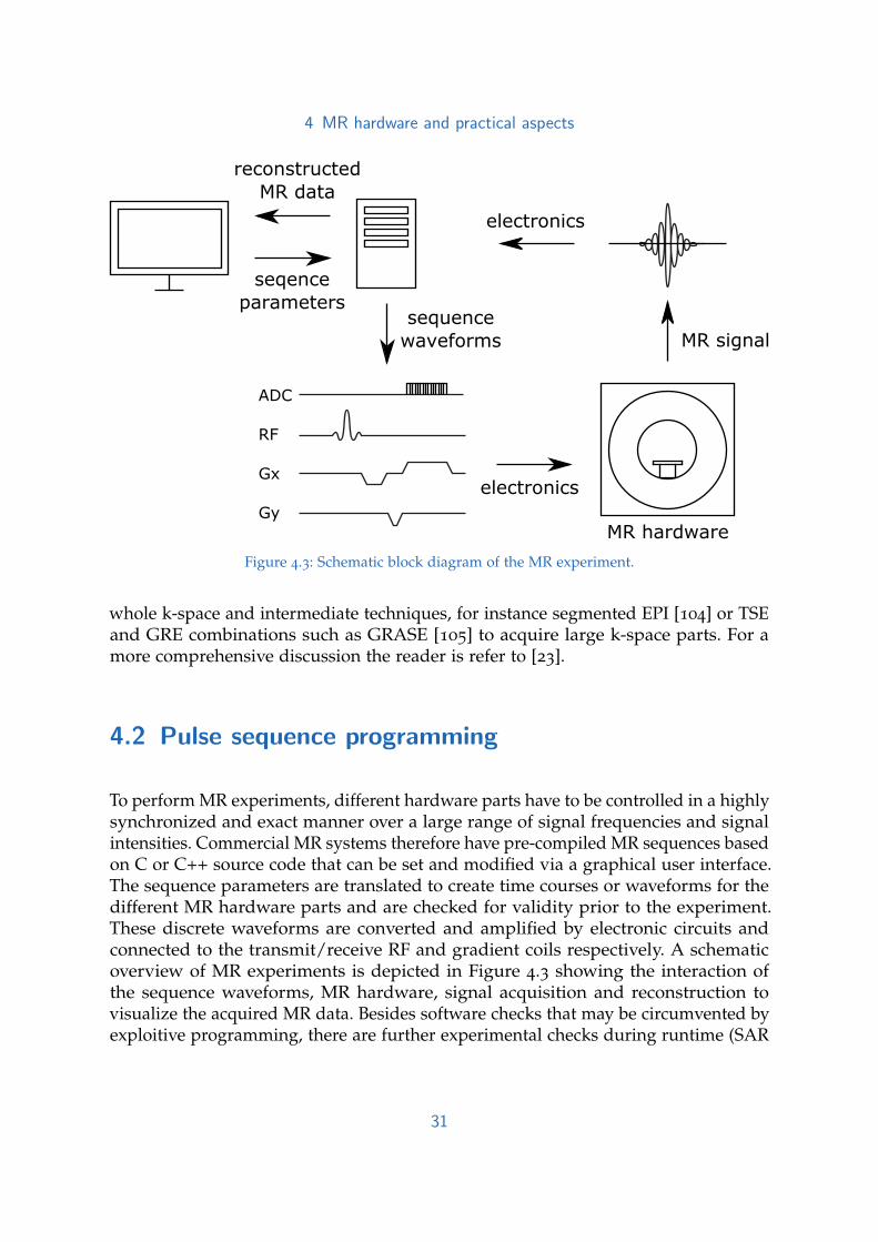
Figure 4.3: Schematic block diagram of the MR experiment.
whole k-space and intermediate techniques, for instance segmented EPI [104] or TSEand GRE combinations such as GRASE [105] to acquire large k-space parts. For amore comprehensive discussion the reader is refer to [23].
4.2 Pulse sequence programming
To perform MR experiments, different hardware parts have to be controlled in a highlysynchronized and exact manner over a large range of signal frequencies and signalintensities. Commercial MR systems therefore have pre-compiled MR sequences basedon C or C++ source code that can be set and modified via a graphical user interface.The sequence parameters are translated to create time courses or waveforms for thedifferent MR hardware parts and are checked for validity prior to the experiment.These discrete waveforms are converted and amplified by electronic circuits andconnected to the transmit/receive RF and gradient coils respectively. A schematicoverview of MR experiments is depicted in Figure 4.3 showing the interaction ofthe sequence waveforms, MR hardware, signal acquisition and reconstruction tovisualize the acquired MR data. Besides software checks that may be circumvented byexploitive programming, there are further experimental checks during runtime (SAR
31

4 MR hardware and practical aspects
and gradient watchdog) to prevent a possible violation of safety or hardware limits.The most common and relevant ones are listed in Table 4.3 for two MR systems.
MR vendors give researchers the opportunity to set up and test their own source codewhich in general allows design of custom sequences and acquisition of preliminarydata, or to check simulations with different timings using custom RF pulse or sliceselective gradient shapes. The sequence programming environments and availablesource codes differ a lot between the different vendors and although most vendorsargue that they offer an open source software environment, in practice their sourcecode is only available after signing specific research agreements which limits theability for rapid prototyping. Even with access to the source codes, the complexity ofthe code and the sensitive software environments in combination with very limiteddocumentation and debugging capabilities often results in large time delays. Recently,an open source framework for the development and execution of MR pulse sequences(https://pulseq.github.io/) was proposed to overcome these hurdles. This toolreads an open source file format and allows interpretation of MR sequences createdin MATLAB (The MathWorks, Inc., Natick, Massachusetts, United States) with theopen source MRI simulation (JEMRIS, http://www.jemris.org/, [58]).
The later presented numerically designed RF and slice selective gradient shapes areexperimentally validated with GRE and SE MR sequences on two 3 T MR scanners(Magnetom Skyra-XQ and Magnetom Prisma-XR, Siemens Healthcare, Erlangen,Germany). For this purpose, the C++ source codes (software versions IDEA VD13Aand VE11C) were modified to read external RF pulses and slice selective gradientshapes and the encoding was changed to measure the slice selection direction. Thefollowing paragraph therefore focuses only on the vendor and scanner specificlimitations.
4.3 RF pulse and slice selective gradient limitations
The layout of the RF and selective gradient shapes is relatively simple and excellentlyfit to the assumption of piecewise constant B-fields, see Section 5. The discretewaveforms, including RF and gradient shapes, are evaluated and matched to acommon time grid defined by the minimal raster time (10 µs for the used MR system,see Table 4.3). For single transmit systems, the RF pulse shape can be defined by asequence of complex piecewise constant blocks with a distinct magnitude and phase.Figure 4.4 shows an optimal SMS RF pulse and slice selective gradient shape [3]normalized to additionally fulfill the software constraints shown in Table 4.3.
32

4 MR hardware and practical aspects
0
0.5
1|R
F| in
a.u
.
0
1
2
3
angle
(RF
) in
rad
time in ms
0 0.05 0.1 0.15 0.2 0.25 0.3
0
0.5
1
gra
die
nt in
a.u
.
Figure 4.4: Optimal SMS RF pulse (Row 1 shows the magnitude and Row 2 the phase) and sliceselective gradient shape used for the experimental validation in [3].
Conventional RF pulses are typically computed at runtime by evaluation of analyticalfunctions, for instance Hamming filtered SINC or Gauss functions, see Section 5, fora desired pulse duration, number of sample points and RF bandwidth.
The discrete RF pulse shapes are scaled at runtime depending on the normalized RFpulse amplitude integral ARF, pulse duration T, desired flip angle φ and temporaldiscretization to compensate coil loading effects. The amplitude integral ARF isdefined as
ARF =
√√√√( N
∑m=1
rm cos θm
)2
+
(N
∑m=1
rm sin θm
)2
, (4.3)
where N is the number of sample points, rm is the normalized RF pulse magnitude andθm is the phase of each time point m. It should be noted that the Eq. 4.3 is independentof the temporal discretization. The temporal settings are defined together with thedesired flip angle by the MR sequence.
The actual RF pulse waveform is amplified at runtime with respect to a reference scanperformed at the beginning of each MR experiments. This reference scan calibratesthe RF transmitter to achieve a 180 flip angle with a rectangular RF pulse with aduration of T = 1 ms. This calibration step compensates field fluctuations caused bycoil loading which depends on the coil, but also on the geometry and material of the
33

4 MR hardware and practical aspects
used phantom or body part [106], [107]. Therefore, numerically designed RF pulsesare normalized to 1 and scaled with the experimentally determined reference scan.Special care has to be taken to define consistent discretisation, flip angle and pulseduration in the MR sequence.
For real valued RF pulses the scaling is straight forward and can be done analogousto conventional RF pulses via the RF pulse amplitude integral given in Eq. 4.3. Forphase modulated RF pulses, however, for instance SMS pulses with an even numberof symmetric slices, the amplitude integral computation, see Eq. 4.3 would becomeclose to zero. This is a result of RF symmetry and would result in a wrong and fartoo large transmit voltage factor, hence producing a wrong field in coil. This can becompensated by relating B1,max directly to the reference scan by a manual calculationof the amplitude integral
ARF,V =Nφ
360TγB1,max, (4.4)
with the number of discrete samples N, the flip angle φ in , the pulse duration T, thegyromagnetic ration γ and the maximal B1 magnitude B1,max. Based on the linearityassumptions of the RF amplifier and the reference scan performed in the calibrationstep before MR data acquisition.
Arbitrary RF pulse shapes (normalized magnitude and phase vector) can be importedto MR sequences in different ways. The most straight forward and safest with respectto reproducibility and validity is a direct numerical import into the sequence sourcecode. This comes with the hurdle that a change of the RF pulse requires a sequencecompilation, a lengthy and error-prone step. Higher flexibility can be achieved bystoring the RF pulses in external RF pulse containers or supply them in exchangeableexternal text or binary files that allows to change RF pulses independently to the MRsequence. It should be kept in mind that for Siemens systems RF pulse containers andtheir shapes are loaded and set up during the booting of the MR scanner. Changing anexisting RF pulse during runtime therefore does not change the RF pulse and requiresa scanner reboot. The most flexible form for rapid prototyping is the inclusion ofexternal files containing the RF and slice selective gradient vectors. These files can beautomatically created with an appropriate header containing additional informationsuch as the amplitude integral, number of sample points or on the timing.
In order to align the RF pulse with other sequence objects, for instance the sliceselective gradient or additional phase objects to perform RF spoiling or off-resonantfrequency shifts, the start and end-time of the RF pulses have to match the gradientraster time of the MR system (for Siemens: 10 µs). The minimal raster time of RFpulses of 25 ns however is much smaller, which would allow to use much finerresolved RF pulses. The piecewise constant normalized slice selective gradient shape
34
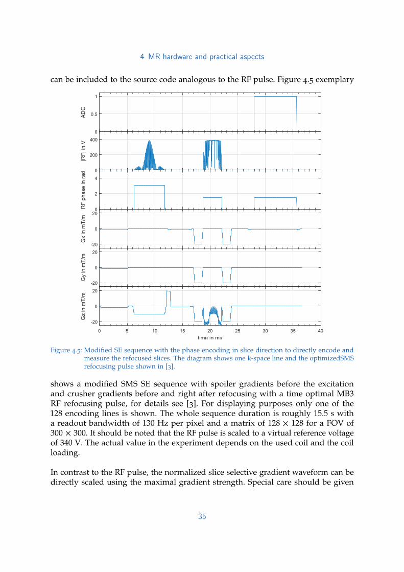
4 MR hardware and practical aspects
can be included to the source code analogous to the RF pulse. Figure 4.5 exemplary
0
0.5
1
AD
C
0
200
400
|RF
| in
V
0
2
4
RF
phase in r
ad
-20
0
20
Gx in m
T/m
-20
0
20
Gy in m
T/m
time in ms
0 5 10 15 20 25 30 35 40
-20
0
20
Gz in m
T/m
Figure 4.5: Modified SE sequence with the phase encoding in slice direction to directly encode andmeasure the refocused slices. The diagram shows one k-space line and the optimizedSMSrefocusing pulse shown in [3].
shows a modified SMS SE sequence with spoiler gradients before the excitationand crusher gradients before and right after refocusing with a time optimal MB3RF refocusing pulse, for details see [3]. For displaying purposes only one of the128 encoding lines is shown. The whole sequence duration is roughly 15.5 s witha readout bandwidth of 130 Hz per pixel and a matrix of 128 × 128 for a FOV of300 × 300. It should be noted that the RF pulse is scaled to a virtual reference voltageof 340 V. The actual value in the experiment depends on the used coil and the coilloading.
In contrast to the RF pulse, the normalized slice selective gradient waveform can bedirectly scaled using the maximal gradient strength. Special care should be given
35

4 MR hardware and practical aspects
not to violate the minimal raster time and the maximal amplitude and slew rateconstraints of the slice selective gradient amplifier. These parameters are evaluatedbefore and during the actual MR scan, thus presenting a potential pitfall. The usedRF pulse and slice selective gradient shapes have a strong influence on the sequencetiming and the validity of the sequence. Therefore, validity should be checked toprevent hardware errors that may result in scanner reboots. There are differentlimitations that are specific for the software and hardware version and these influencethe RF pulse design. Table 4.3 summarizes the most important software and hardwarelimitations for Siemens IDEA VD13A/VE11C and the Siemens Skyra-XQ 3 T MRscanner used later on. The change of the read-out gradient from the phase encoding
Table 4.3: Overview of the important software and hardware (Skyra-XQ) constraints for MR sequenceprogramming. Ns denotes the maximal number of discrete sample points, rm the normalizedRF magnitude, θm the RF phase, Gs,m the normalized slice selective gradient amplitude, τRFthe RF raster time and τGs the gradient raster time.
software constraints hardware constraints
Ns 8192 min τRF 25 nsrm 0− 1 min τGs 10 µsθm 0− 2π min RF hold duration 8 µsGs,m −1− 1 min Gs rise time 5.55 µs mT−1 m−1
max Gs 24 mT m−1 max Gs 43 mT m−1
max Gs 180.18 T m−1 s−1 max Gs 200 T m−1 s−1
min τRF 25 ns max RF power 29.7 kWmin τGs 10 µs max RF bandwidth 800 kHz
to the slice direction allows measurement and visualization of the excited slices [3].The result is a phase encoding along the slice direction, thus obtaining the spatialdependent signal.
Besides obvious imperfections such as B0 and B1 variations or non-linear gradientsacross the field of view [23], [25], [108], the time varying RF and slice selectivegradient shapes may further deviate from the theoretical waveforms. The slope ofthe RF and slice selective gradient shapes are implemented as piecewise constantfunctions, see Section 4.2, which cannot be exactly realized by the amplifiers andcoils due to an inherent low pass characteristics. Furthermore, the RF and gradientamplification have different frequency content and power which makes them notdirectly comparable. For an extensive review the reader is referred to [109] for RFand [39] for gradient amplification.
The discrete RF signals are converted into analogue signals and modulate the ampli-fied RF-transmitter signal in order to create RF fields in the µT range. For human in
36

4 MR hardware and practical aspects
vivo MR systems the RF power lies in the range of 0.5− 35 kW [109]. RF amplifierimperfections may alter the discrete pulse amplitude and phase slopes, thus resultingin potential slice profile degradation and alterations. Most of these RF amplifiernon-linearities can be corrected by a pre-distortion of the RF shape [110]. The use ofhighly modulated complex RF pulses however can result in unwanted slice profileartifacts, whereas real valued RF pulses create less artifacts [111]. In general, theeffective RF bandwidth outperforms the bandwidth achievable by the gradient systemand alterations on the RF shape should be minimal [3].
The gradient system on the other hand typically has much more restricted bandwidthlimitations in the range of several tenths of kHz thus potentially impacting rapidlyvarying slice selective gradient slopes. These limitations results from the need forhigher currents to produce the gradient waveforms [112] and eddy current effects[113], [114]. The overall alterations can be measured and modeled by the gradient im-pulse response function (GIRF) [115]–[117]. It should be further kept in mind that thegradient bandwidth is highly vendor specific and time varying gradient forms resultin different alterations on different systems [3], [111], [115]. The actually producedslice selective gradient waveform Gs,GIRF(t) can be computed by a convolution
Gs,GIRF(t) = Gs(t) ∗ GIRF(t), (4.5)
of the ideal slice selective gradient shape Gs(t) and the measured or modelledGIRF. The impact of the GIRF is comparable to a low-pass effect with a runtimedelay resulting in a smoothed and time shifted slice selective gradient shape whichalters the slice profile accuracy. However, knowledge of the GIRF allows iterativecorrection of the RF pulse [118] for non-ideal gradient distortions. The GIRF can bealso incorporated directly in the OC pulse design [119], see Section 7. This allows touse the OC based constrained joint design of RF and slice selective shape for systemswith a limiting gradient amplifier bandwidth [119].
37

5 RF pulse design
Contents
5.1 RF pulse categories . . . . . . . . . . . . . . . . . . . . . . . . . . 39
5.2 Spatial non-selective RF pulses . . . . . . . . . . . . . . . . . . . 41
5.3 Spatial selective RF pulses . . . . . . . . . . . . . . . . . . . . . . 44
5.4 Variable-rate selective excitation . . . . . . . . . . . . . . . . . . . 51
5.5 SMS RF pulse design . . . . . . . . . . . . . . . . . . . . . . . . . 52
5.5.1 Peak RF amplitude reduction . . . . . . . . . . . . . . . . . 53
5.5.2 Peak RF amplitude and RF power reduction . . . . . . . . . 56
5.6 Slice selective RF pulse design via optimal control . . . . . . . . . 59
5.6.1 Single slice selective RF pulse design via OC . . . . . . . . . 60
5.6.2 SMS RF pulse design via OC . . . . . . . . . . . . . . . . . 68
RF pulses and gradients are key factors and essential for most MR experiments. RFpulse design summarizes how to compute waveforms for the RF and gradient systemthat change the magnetization from a given initial state to a desired state with respectto different parameters, including profile accuracy, amplitude restrictions and safetyconstraints. This work mainly focusses on one dimensional slice selective RF pulsesfor single transmit to excite or refocus one dimensional slice profiles.
This section discusses different approaches to design RF pulse and slice selective gra-dient shapes for single- and SMS applications. For simplicity reasons, the followingsections use the rotating frame of reference. This implies, that for experimental appli-cation, the RF pulses have to be modulated with the Lamor frequency with respectto the main field, see Eq. 2.5. Figure 5.1 shows this relationship for a rectangular RFpulse.
The focus of this thesis lies on the design of RF and slice selective gradient waveformsvia optimal control theory, it’s application to SMS imaging and the experimentalvalidation. The first part of this section introduces and compares different RF pulse
38

5 RF pulse design
f in Hz
amplitude
in a.u
0
amplitude
in µT
time
in s
f in Hz
amplitude
in a.u
20
amplitude
in µT
time
in s
B1 cos(20t)
T
T
1/T
1/TB1
B1B1 sin(20t)
Figure 5.1: RF pulse in the rotating frame of reference (Row 1) and in the laboratory frame of reference.Please note, that the magnitude remains unchanged.
design methods that were used to initialize and benchmark the optimized resultspresented in [1]–[3] and the Appendix. The main results of these works are introducedand summarized at the end of this section.
5.1 RF pulse categories
The most basic RF pulses can be summarized in four main categories: excitation,inversion, saturation and refocusing [23]. The description and visualization of RFpulse categories is straight forward and can be formulated in the magnetization [120]or spin domain [66]. Although the spin domain description with the Cayley-Kleinparameters appears to be more complicated, elegant transformations exist to assessthe main RF classes and transform their result to the other domain respectively [66].These relations and transformations are summarized in Table 5.1. It should be noted,that the perfectly crushed refocusing scenario, where the FID of refocusing pulseis assumed to be perfectly de-phased, can be easily described in the spin domainby setting α to zero such that it does not contribute to the transverse magnetization.The later described optimal control (OC) approaches use the magnetization domainformulation for excitation [1] and the spin domain formulation for perfectly crushedrefocusing [2], [3], see also the Appendix. Figure 5.2 gives a graphical overview of
39

5 RF pulse design
Table 5.1: Response of the Magnetization to commonly used RF Pulse Types in Terms of the Cayley-Klein Parameters, adopted from [23]
Initial ConditionPulse Type (Mx, My, Mz)T Final state
Excitation or saturation (0, 0, M0)T Mx = 2M0Re(αβ?)
My = 2M0 Im(αβ?)Mt = 2αβ?
Inversion (0, 0, M0)T Mz = M0(1− 2|β|2)
Refocus (M0, 0, 0)T Mt = M0((α?)2 + β2)
Refocus (perfect crusher) (M0, 0, 0)T Mt = M0β2
φB1
B0
y'
x'
z
M0
M φB1
B0
y'
x'
z
M0
M
B1
B0
y'
x'
z
M0
M(2)
M(1)
excitation inversion refocusing
Figure 5.2: Most common RF pulse categories (excitation, inversion and refocusing) and their desiredtrajectory of the isocenter magnetization.
three RF pulse categories. For simplicity reasons, this is shown only for one perfectlyon-resonant spin in the isocenter.
The concept of one dimensional slice selective RF pulse design can be easily extendedto multiple dimensions, see [23], for instance to design RF pulses that excite, refocusor saturate two or three dimensional shapes [42]–[49]. Analogous, this idea can befurther extended to compute spatially spectral RF pulses [121]–[123]. A relativelysimple and direct extension to the basic pulse categories introduced above are com-posite RF pulses [23], [38], [110], a series of non-selective RF pulses with or withoutvarying phase that are commonly used in NMR applications, for instance broadbandexcitation [124], WALTZ-16 [125] decoupling, or saturation at distinct frequencies[38], [126]. Moreover, special RF classes developed over time, such as velocity com-pensating excitation [127], velocity selective excitation [128] or myocardial tagging(SPAMM [129] and CSPAMM [130]) by an application of alternating non-selective RFblocks and slice selective gradient blips. This alternating application scheme and the
40

5 RF pulse design
corresponding replicating excitation pattern form the fundamentals of the PINS [131]method developed for SMS imaging. A completely different RF pulse category areadiabatic RF pulses [23], [38], [110]. Their main advantage is an inherent B1 robustnesswith the hurdle of large RF power requirements. Since adiabatic pulses are not themain focus of this work, the reader is referred to [23], [110] for additional informationon this topic. Besides the RF pulse type, parallel transmit (pTx) [132]–[135] allowsthe use of independent RF channels to directly address B1 and local SAR issues[136]–[139].
RF pulses alter the magnetization from a given initial magnetization as close aspossible to a desired magnetization (for instance from M0 = (0, 0, M0)
T to Mdes =(0, M0, 0)T for an ideal 90 excitation RF pulse). This process can be defined inthe frequency or spatial domain for non-selective and slice selective applicationsrespectively. Conventional RF pulse design based on analytical RF waveforms typicallyenables choice of only a limited number of parameters, for instance the pulse durationT, nominal time bandwidth product (TBWP), slice thickness (THK) defined on thefull width at half maximum (FWHM), or maximal error deviations (e1 and e2). TheTBWP of SINC based pulses can be approximated
TBWP = T∆ f (5.1)
with the pulse duration T and the bandwidth of the main lobe ∆ f . Alternatively, theTBWP is directly given by the number of zero crossings [23].
RF pulse design based on optimization methods further allows assessment andpredefinition of more parameters. For instance, the spatial domain can be treatedpoint-wise in space to define a desired magnetization for all spatial points. Figure 5.3summarizes four different design approaches for rectangular, SINC, SLR and opti-mization based RF pulse design. Additionally to these state constraints, optimizationbased methods typically allow to further define limitations on the RF pulse and sliceselective gradient shape, for instance the maximal amplitudes or time derivatives[2], [3]. It should be noted, that most RF pulse methods typically assume a constantslice selective gradient while OC based methods, presented in Section 5.6, enablesimultaneous design of the RF and slice selective gradient.
5.2 Spatial non-selective RF pulses
Even in the most basic NMR experiment, the creation of a FID signal without a spatialvarying gradient, RF pulses typically can not be analytically designed. There are
41

5 RF pulse design
M0
magnetization
f in HzFWHM ~1.21/T
M0
magnetization
f in HzFWHM ~TBWP/T
M0
magnetization
f in Hz
e1
e2
M0
magnetization
z in mdz
a)
c) d)
bb)
Mx(z)
My(z)
Mz(z)
Mt(T,φ)
Mt(TBWP, φ
T, e1, e2)
Mt(T,φ)
FWHM ~TBWP/T
Figure 5.3: Parametrized and pointwise discription of the desired magnetzation in slice selectiondirection for a rectangular (a), SINC (b), SLR (c) and optimization (d) based RF pulsedesign method.
two problems which prevent an analytical solution, a coupling of the transversaland longitudinal component and inherent relaxation effects. However, neglectingthe relaxation terms decouples the Bloch equations. The additional assumptionsof a perfectly homogeneous B0 field and an absent slice selective gradient, allowsfor a geometric description of the rotating magnetization vector, see Section 2.3.To visualize the off-resonance behaviour of spatial non-selective RF pulses, theassumption of a constant slice selective gradient amplitude maps the spatial variablez to the corresponding frequency f (z). The frequency can be computed as
f (z) =γ
2πGsz, (5.2)
with the gyromagnetic ratio γ/(2π) of the used nuclei in MHz T−1, the time constantamplitude of the slice selective gradient Gs in mT m−1 and the spatial position zin m. It should be noted, that this relies on the assumption of a spin ensemblewith a uniform frequency distribution, according to Eq. 5.2. In the following sectiononly rectangular pulses are discussed. For a more extensive comparision of non-selective RF pulses, including composite pulses, adiabatic pulses (for instance half-,full-passage or BIR pulses) or optimized block pulses, the interested reader is referredto [140].
42

5 RF pulse design
Rectangular RF pulses are fully described by the B1 amplitude, the Lamor frequencyand the pulse duration T resulting in the flip angle, see Eq. 2.26 and Section 2.3.A simple example can be found using the gyromagnetic ratio of hydrogen protonsγ = 2.6731 × 10⁸ rad s−1 T−1, a pulse duration T = 1 ms and a desired flip angle ofπ/2 to compute the required B1 amplitude according to
B1 =φ
γT= 5.876µT. (5.3)
In order to minimize relaxation effects and the minimal achievable echo time, the RFpulse duration should be typically as short as possible.
Although an infinitely high and short rectangular RF pulse would be desirable, the RFpower amplifier constraints limit the achievable maximal field strength and thereforelimit the minimal RF duration. See Section 4 for the description of how the B1 field isconnected to the voltage of the RF amplifier.
Two rectangular RF pulses (π/8 and π/2) are shown together with a two-sided FFTand Bloch simulations in Row 1 of Figure 3.2. It can be seen, that for this smalltip angle RF pulse both simulations result in comparable slice profiles. However,it should be noted that although there is no clear visual difference between theseresults, they are not numerically identical. Using the small tip angle approximation,rectangular RF pulses result in SINC-shaped excitation profiles whose full half widthmaximum and zero crossings are defined by the pulse duration and the FWHM canbe approximated by 1.21/T [23]. For the shown π/8 pulse this results in a FWHMof 10.37 kHz which fits nicely to the simulations given in Figure 3.2. The frequencyselectivity of non-selective pulses is mainly determined by the pulse duration, themain parameter for the desired magnetization, see Figure 5.3, and the RF waveform.The prominent side-lobes of rectangular pulses can be suppressed using Gaussianpulses, see Section 5.3 with the drawback of lower frequency selectivity.
Increasing the flip angle to π/2 for the same maximal B1 amplitude (B1,max = 12.5µT) requires to increase the pulse duration T = 0.47 ms to be 4 times longer. Theπ/2 RF pulse and the corresponding forward FFT simulations are shown in Row 2
of Figure 3.2. Now, the small tip angle approximation is violated and a significantdifference between FFT and Bloch simulations is the result. Compared to the π/8example, the longer pulse duration additionally leads to a more selective excitationprofile. The small tip angle approximation results in a FWHM of 1.3 kHz, whilethe Bloch simulation shows a merely smaller FWHM of roughly 1.1 kHz. Althoughrectangular RF pulses could be also used for slice selective applications, their poorslice profile limits the practical value for slice selective applications. Nevertheless,they are commonly used for spatial non-selective NMR and MRI applications.
43

5 RF pulse design
5.3 Spatial selective RF pulses
To achieve a spatially selective RF pulse, a slice selective gradient is applied simulta-neously with the RF field.
All spins in the object of interest are acquired simultaneously during signal acquisitionand a de-phasing across the slice selection direction would results in a reduced FIDsignal. Therefore, the phase across the slice is an important parameter to characterizeslice profiles. Slice selective RF pulses for conventional GRE or SE imaging preferablytilt the magnetization uniformly across the slice selection axis. However, specializedapplications such as peak power reduction [141], [142] may benefit from a de-phasedslice profile. Using the complex description of the magnetization the phase θ can becomputed with
θ(z) = tan−1 Im(Mxy(z))Re(Mxy(z))
, (5.4)
for the spatial position z. In the context of slice selective RF pulses, the use of aslice selective gradient inherently results in a de-phasing of the magnetization in thetransversal plane. For linear-phase RF pulses, for instance SINC (Section 5.3), Gauss(Section 5.3) or SLR (Section 5.3) based RF pulses, the accumulated phase dispersioncan be corrected with a re-phasing gradient. The required gradient area depends onthe isodelay [23] of the RF pulse. For symmetric pulses the isodelay is typically halfthe RF duration, for SLR or optimized RF pulses the iso-delay may further dependon the flip angle. Besides linear-phase RF pulses, the SLR design method allowscomputation of maximal-phase with a larger iso-delay or minimal-phase pulses witha smaller iso-delay [43]. Although these pulses typically suffer from a worse sliceprofile, their phase properties allow for a direct use in saturation or in the contextof minimal TE since less refocusing area is required. Figure 5.4 summarizes a linear-phase SLR pulse without (Column 1) and with (Column 4) a matched slice selectivere-phasing gradient. Column 2 shows a maximal-phase SLR pulse, intended for theuse of saturation with an even higher de-phasing, compared to Column 1. Column3 shows a minimal-phase SLR pulse where a reduced refocusing area is required,thus enables reduction of the TE. The minimal- or maximal-phase pulses should notbe confused with non-linear-phase pulses such as quadratic [142] or quasi randomphase RF pulses. In contrast to the residual linear-phase, a non-linear-phase cannotbe corrected by a slice selective gradient. However, the use of two consecutive RFpulses with the same non-linear-phase results in a phase cancellation and allows theuse of non-linear pulses, for instance in double refocused diffusion or matched spinecho sequences [143], [144].
44

5 RF pulse design
time in ms
0 2 4B1
in µ
T a
nd
Gs
in m
T/m
-10
0
10
SLR
distance in m×10-3
-2.5 0 2.5no
rma
lize
d m
ag
ne
tiza
tio
n
-1
-0.5
0
0.5
1 Mx
My
Mz
time in ms
0 2 4
-10
0
10
SLR
distance in m×10-3
-2.5 0 2.5
-1
-0.5
0
0.5
1
time in ms
0 2 4
-10
0
10
maximal -phase SLR
distance in m×10-3
-2.5 0 2.5
-1
-0.5
0
0.5
1
time in ms
0 2 4
-10
0
10
minimal -phase SLR
distance in m×10-3
-2.5 0 2.5
-1
-0.5
0
0.5
1
B1,x
B1,y
Gs
Figure 5.4: Overview of slice selective SLR based RF pulses with constant slice selective gradientshapes and the Bloch simulations. Column 1 shows the linear de-phasing that is correctedin Column 4 with a slice selective re-phasing gradient. Column 2 shows a maximal-phaseRF pulse for saturation and Column 3 shows a minimal RF pulse with decreased gradientrefocusing lobe for minimal TE purposes.
SINC pulses
The Fourier transform of a rectangular function in one domain results in an infiniteSINC-function in the transformed domain. Assuming the small tip angle approxima-tion, SINC-shaped RF pulses therefore excite rectangular slice profiles. The RF pulseshape B1(t) can be easily defined using the SINC function:
B1(t) =
sin πt
πt if t 6= 0,1 if t = 0,
(5.5)
using t = −TBWP: τ :TBWP to compute a B1(t) with the intended frequencyselectivity based on the TBWP and the discretization step τ. However, there aretwo problems associated with the use of SINC pulses. First, the aforementionedassumption only holds for small flip angles. Second, the SINC function is defined foran infinite temporal duration which is not feasible due to limited TE and RF amplifierrequirements. Since the RF area defines the flip angle in the iso-center, the limitedB1 amplitude results in longer RF durations. This results in an inherent trade-offbetween frequency selectivity and pulse duration.
45
5 RF pulse design
The selectivity of a SINC pulse is defined by the dimensionless TBWP, see Eq. 5.1.Together with a limited B1,max, the choice of the TBWP is a crucial decision thatstrikes a balance between RF pulse duration and slice profile fidelity. Similar torectangular block pulses, see Section 5.2, there are useful approximations to definethe bandwidth or slice profile thickness with respect to the FWHM of SINC basedRF pulses [23] . As an example, Figure 5.5 shows a SINC based RF pulse with3 zero crossings, that correspond to TBWP = 3. The pulse duration is scaled toT = 2.644 ms to perform a 90 excitation with B1,max = 12.5 µT, see Eq. 2.25 Fora time-constant slice selective gradient, the slice thickness THK can be chosen byscaling the amplitude of the slice selective gradient. According to Eq. 4.2 a THK of 5mm results in Gs = 10.461 mT m−1, which is confirmed by the Bloch simulations inFigure 5.5. Jump discontinuities at the beginning and end of the RF pulse result inclearly visible and severe ripples in both the slice profile and the out-of-slice profile.This effect is similar to leakage in digital signal processing and can be reduced byfiltering the RF waveform with proper window functions such as Hamming or Hannwindows. Column 2 of Figure 5.5 summarizes the effect of an Hamming window(shown dotted) on the SINC based RF pulses shown in Column 1. It can be clearlyseen, that the unwanted ripples are reduced with the drawback of a simultaneousreduction of the slice profile transition steepness or TBWP. This is strongly connectedto digital signal processing and results in a trade-off between frequency selectivity andleakage suppression. Nevertheless, and mainly due to their simplicity and analyticaldescription, windowed SINC functions are still the most used RF pulse shapes forsmall flip angles in slice selective MR experiments.
Gaussian pulses
Comparable to SINC pulses, Gaussian pulses are another special case of analyticalRF pulse types that originate from the small tip angle approximation. Gaussian RFpulses can be designed analytically by
B1(t) = B1,maxe−t2/(2σ2), (5.6)
with the time-vector t running from −T/2 to T/2 with T being the pulse duration[23]. The variance σ2 is used to adjust the desired frequency selectivity. The Fouriertransform of a Gauss function is another Gauss function with a favourable smoothdecline of the slice profile.
46

5 RF pulse design
time in ms
0 2 4B1
in µ
T a
nd
Gs
in m
T/m
-10
0
10
SINC
distance in m×10-3
-2.5 0 2.5no
rma
lize
d m
ag
ne
tiza
tio
n
0
0.5
1
time in ms
0 2 4
-10
0
10
Hann filtered SINC
distance in m×10-3
-2.5 0 2.5
0
0.5
1
time in ms
0 2 4
-10
0
10
SLR
distance in m×10-3
-2.5 0 2.5
0
0.5
1
time in ms
0 2 4
-10
0
10
SLR VERSE
distance in m×10-3
-2.5 0 2.5
0
0.5
1Mx
My
Mz
B1,x
B1,y
Gs
Figure 5.5: Overview of slice selective RF pulses designed with the Fourier approximation (Column1 and 2) and SLR (Column 3 and 4). Column 2 shows a Hamming windowed version(dotted line) of the pulse shown in Column 1 and Column 4 shows a VERSE’d version(with prescribed gradient shape) of Column 3 respectively.
Shinnar–Le Roux algorithm
The SLR algorithm does not rely on the small tip angle approximation and can beused for accurate large flip angle RF pulse design. It is formulated in the spin domainwith neglected relaxation terms and makes use of the hard pulse approximation, seeSection 3.1.3. Then, the rotation for each time point can separated for RF and sliceselective gradient as
Qm =
(Cm −S?
mSm Cm
)(z1/2 0
0 z−1/2
), (5.7)
with Cm = cos(γ|B1,m|τ/2), Sm = iei 6 B1,msin(γ|B1,m|τ/2) describing the effect of theRF pulse and z = eiγGxτ describing the effect of the slice selective gradient G at thespatial position x. Using Eq. 5.7, the recursion to compute the accumulated rotation,see Eq. 3.27, becomes(
αmβm
)= z1/2
(Cm −S?
mSm Cm
)(1 00 z−1
)(αm−1βm−1
), (5.8)
47

5 RF pulse design
with the Cayley-Klein parameters αm and βm for each time step m. The definition oftwo complex polynomials Am = zj/2αm and Bm = zj/2βm defines the forward SLRtransform (
AmBm
)=
(Cm −S?
mz−1
Sm Cmz−1
)(Am−1Bm−1
). (5.9)
Starting with (A0, B0)T = (1, 0)T, see Eq. 3.28, the polynomials for the nth step An
and Bn are complex polynomials in z−1
An(z) = ∑n−1m=0 amz−m,
Bn(z) = ∑n−1m=0 bmz−m,
(5.10)
of order n− 1. The forward SLR transformation (Eq. 5.9) computes An(z) and Bn(z) ofan arbitrary piecewise constant RF pulse. For small tip angles the SLR transformationcan be reduced to the z-transform [66].
The idea leading to SLR based RF pulse design is to invert the forward SLR transformand use two complex polynomials An(z) and Bn(z) to calculate the RF pulse thatcreates these polynomials. The inversion of Eq. 5.9, or inverse SLR transform, is givenby (
Am−1Bm−1
)=
(Cm S?
m−Smz Cmz
)(AmBm
)=
(Cm Am + S?
mBmz(−Sm Am + CmBm)
). (5.11)
It can be proven [66] that the relation
Bm,0
Am,0=
Sm
Cm=
ieiθmsinφm/2cosφm/2
, (5.12)
can be used to compute the RF waveform for each time point
B1,m =1
γτφmeiθm , (5.13)
with the rotation angle φm and the RF phase θm
φm = 2tan−1 | Bm,0/Am,0 |,θm = 6 (−iBm,0/Am,0),
(5.14)
where Am,0 and Bm,0 are the lowest order of the polynomials.
The SLR based RF pulse design consists of two main steps. After the design ofthe filter polynomials Bn(z) and An(z), the inverse SLR transform computes thecorresponding RF pulse.
48
5 RF pulse design
To design a 90 excitation pulse, the polynomial Bn(z) should be as close as possibleto an ideal rectangular slice profile with the in-slice amplitude for φ = 90
Bd(z = eiγGxτ) = i(nx + iny)sinφ/2 = isinφ/2 = i√
2/2 (5.15)
and the out-of-slice amplitude for φ = 0
Bd(z = eiγGxτ) = isinφ/2 = 0. (5.16)
However, rectangular functions cannot be described exactly by the Bn(z) polynomial.The goal is to find a polynomial approximation Bn(z) close to the ideal slice profilewhich can be computed with different filter design methods including the Parks-McClellan algorithm (equi-ripple error) or by a least squares approach [66]. It can beshown that the FIR filter design parameters d1, d2, and the two cut-off frequencies forpass- and stop-band directly relate to slice profile accuracy, frequency selectivity andintended RF pulse category [66]. After Bn(z) has been designed, the magnitude ofthe polynomial An(z) can be computed by
|An(z)| =√
1− Bn(z)B?n(z) (5.17)
using the magnitude constraint |An(z)|2 + |Bn(z)|2 = 1. In order to get low RFenergy requirements [23] the phase of the polynomial An(z) is typically set to fulfil aminimum-phase solution. Finally, the corresponding RF pulse can be computed by theinverse SLR transform of the polynomials An(z), Bn(z). Figure 5.6 gives an overviewof the different SLR design steps and shows the two polynomials An(z), Bn(z) andthe resulting RF pulse together with the corresponding profiles. The symmetricSLR RF pulse results in a linear de-phasing across the slice direction that can berecovered with a slice selective refocusing gradient. Other phase patterns can beachieved choosing a non-symmetric (minimum and maximum phase) or complexBn polynomial. Column 3 of Figure 5.5 shows a representative SLR excitation pulse(φ = 90 , N = 256, T = 2.894 ms, TBWP= 3, d1 = 0.01/4, d2 = 0.01/
√(2), linear-
phase, least squares filter design method) together with a constant slice selectivegradient and the forward Bloch simulation.
Although the overall RF pulse slope is similar to the SINC based RF pulses, theslice profile is closer to the desired rectangular shape. Efficient digital filter designmethods allows rapid design of RF pulses and makes the SLR the gold standard forlarge tip angle design with constant slice selective gradient and neglected relaxationterms [66].
49

5 RF pulse design
normalized time
0 0.2 0.4 0.6 0.8 1
-0.02
0
0.02
0.04
0.06
Bn polynomial
Re
Im
normalized position
-0.2 -0.1 0 0.1 0.2
0
0.5
1
Bn and B
d profile
Bn
Bd
normalized time
0 0.2 0.4 0.6 0.8 1-0.5
0
0.5
1
An polynomial
Re
Im
normalized position
-0.2 -0.1 0 0.1 0.2
-1
0
1
An profile
Re
Im
normalized time
0 0.2 0.4 0.6 0.8 1-0.05
0
0.05
0.1RF pulse
Re
Im
normalized position
-0.2 -0.1 0 0.1 0.2-0.5
0
0.5
1
excitation profile
Mx
My
Figure 5.6: Overview of the different stages of the SLR Pulse design for a 90 excitation pulse. The Bnpolynomial is designed with a least squares approach to fit to the desired slice profile Bd.An is computed based on Bn with a minimal phase constraint. Both polynomials result inthe complex RF pulse using the inverse SLR transform. The results of the Bloch simulationswith corrected linear phase dispersion shows the final Mx and My components.
Additional RF design methods
In addition to the above described RF design methods further methods have beenproposed. These include RF pulse design with the continous or discrete inversescattering transform [145], [146] or the design of adiabatic RF pulses [23], [110], [140]together with most of the design methods listed in Section 5.1.
Alternatively, RF pulse design problems can be formulated using optimization tech-niques such as simulated annealing [147], [148], evolutionary approaches [149], [150],neuronal networks [151] or optimal control theory [1]–[3], [47], [49], [120], [152]–[158].For the ease of readability the description of the proposed OC methods are given inSection 5.6. The underlying idea is to formulate a suitable functional and minimize itby finding the external magnetic field, for instance the RF pulse or the slice selectivegradient waveform, based on the Bloch equations measured in different norms. Themain advantage of numerical optimization methods lies in its flexible formulation thatcan be extended and adapted to many different applications with problem specificfunctionals, for instance parallel transmit, SMS or multidimensional modelling, aswell as B1 and B0 robustness. Due to the accurate design model, these numericaldesign methods typically lead to better magnetization profiles with the hurdle ofincreased computational costs, thus in general preventing on the fly design, and
50

5 RF pulse design
more complicated numerical design. Nevertheless, for single transmit cases RF pulsestypically can be computed off-line and stored in a pulse library on the MR scannerto be selected in the intended MR sequence. However, GPU parallelization has beenshown to reduce the computation time dramatically from the range of hours downto several seconds [159]. This could be highly interesting in the context of paralleltransmit where RF pulses have to be optimized for a patient specific B1 transmitmap.
5.4 Variable-rate selective excitation
So far, the design of RF pulses is based on the assumption of no (Section 5.2) or aconstant spatially variable field gradient (Section 5.3). For neglected relaxation therelation between RF amplitude and slice selective gradient can be exploited to reducethe overall RF power requirements. This is known as variable-rate selective excitationVERSE [160]. The reduction of the overall RF power comes with the drawback ofincreased sensitivity to of off-resonance effects increase due to a time varying sliceselective gradient shape with lower amplitudes. Later implementations extended thisidea to reduce the pulse duration and apply it to reduce the peak RF amplitude [112]and power of SMS pulses [118]. A thoughtful derivation and further elaboration ofVERSE can be found in [23].
To reduce the RF amplitude, a rectangular RF pulse can be stretched in time (seeSection 5.2) which reduces the RF bandwidth. This change in RF bandwidth can becompensated by the same reduction of the amplitude of the slice selective gradient,see Eq. 5.2. This idea can be extended to a time varying RF pulse and slice selectivegradient shape with a transformation function λ(t). The VERSE transformation canbe defined [23] by
B1,VERSE(t) =2π
γGsB1(k)
dkdt
, (5.18)
Gs,VERSE(t) =2π∆ fγ∆z
λ(t) = Gsλ(t), (5.19)
with
k(t) =γ
2π
∫ t
0Gs(t′)dt′ =
γGs
2π
∫ t
0λ(t′)dt′ (5.20)
being the RF k-space trajectory [23]. The transformation in Eq. 5.18 connects λ(t) withthe slope of the RF pulse B1(t) and the constant slice selective gradient amplitudeGs. This transformation results in a variable-rate slice selective gradient shape with a
51

5 RF pulse design
matched RF pulse that compensates the varying k-space velocity. For instance, whenthe slice selective gradient amplitude is small, the RF amplitude has to be reduced tocompensate the slow k-space velocity.
The main question for the VERSE application is the determination of the transfor-mation function λ(t). The tranformation function λ(t) can be defined by a manualselection of time points where the RF amplitude should be reduced, or by an iterativeadaption until all hardware constraints on the RF and slice selective gradient am-plitude and slew rate are fulfilled [112]. This however should not be confused withthe method described in Chaper 5.6 to jointly design RF and slice selective gradientshape with explicit hardware constraints.
Column 4 of Figure 5.5 shows the VERSE’d Hann filtered SLR RF pulse of Section 5.3(re-sampled with a time discretization τ = 2.36 µs, a factor of 10, to reduce theinterpolation artefacts) and λ(t) composed out of two constant blocks and half a Sineperiod at the center where the RF pulse amplitude should be reduced. The area ofthe slice selective gradient has been scaled such that the gradient impact remainsconstant, thus leading to an almost identical slice profile before and after VERSE.
5.5 SMS RF pulse design
Conventional single slice selective MR imaging experiments acquire an integrated MRsignal originating from protons of a specific slice or slab, a process which is repeatedto acquire the entire k-space. Although TE for single- and multi-shot sequences lies inthe sub-second range, the need to fill a spatially encoded two or three dimensional k-space in combination with relatively long T1 times typically results in long repetitiontimes with a long dead time in between. This dead time can be used in conventionalmulti-slice imaging to multiplex the acquisition of spatially non-overlapping slices toincrease the temporal acquisition efficiency [23]. Developments in parallel imagingenabled an extension of this idea of slice selective multi-slice imaging to acquireslice information simultaneously to further increase the acquisition efficiency anduse coil sensitivities to separate the aliased slice information [95], [161]. Althoughthe main idea of SMS was founded in 1988 [162], it took several years until SMSimaging became widely accepted as evidenced in various publications [95], [163]–[166] and pushed by pre-compiled SMS-MR sequences provided by the University ofMinnesota (Center for Magnetic Resonance Research, CMMR) and the MassachusettsGeneral Hospital (MGH, Boston). Today, SMS is commercially available as a clinicallyapproved MRI sequence product.
52

5 RF pulse design
Besides parallel imaging based reconstruction [82], [167]–[172], special RF pulsesthat excite or refocus slices simultaneously are essential for SMS imaging [95]. Thetopic of this section deals with limitations influencing the slice acceleration factor,or multi-band MB factor. Different approaches are introduced to increase the sliceacceleration while maintaining a minimal echo time to maximize the achievable MRsignal.
SMS RF pulses can be computed by a simple superposition of individual RF pulseswith a different carrier frequencies [162]. Originally, the resulting SMS pulses werecombined with Hadamard encoding [161] to disentangle the aliased slice informationby subtraction of raw images acquired with alternating phase patterns [162]. Thisimplies that the required acquisitions to disentangle the aliased slice informationincrease by the power of the MB factor. To avoid multiple acquisitions, later imple-mentations use parallel imaging reconstruction techniques [95]. Slice selective RFpulses, see Section 5.3, can be easily shifted along the slice direction z by a phasemodulation of the RF pulse shape
B1,o f f set(t) = B1(t)eiγGs∆zt, (5.21)
for a given slice selective gradient amplitude Gs at each time-point t [95]. This allowssuperposition of phase modulated RF pulse shapes B1(t) replicated in the slicedirection for the desired spatial locations ∆zn
B1,sp(t) =MB
∑n=1
B1(t)eiγGs∆znt, (5.22)
with MB being the MB factor. This process is depicted in Figure 5.7 for a MB3superposition pulses together with the Bloch simulation to visualize the position ofthe slice profile. The superposition results in a linear scaling of the maximal peak RFamplitude [95], thus easily reaching B1,max and RF power.
5.5.1 Peak RF amplitude reduction
The linear B1 peak amplitude scaling of conventional superposition pulses competeswith RF amplifier constraints, see Section 4. For typical 3 T in vivo MR systems theRF amplifiers are usually limited to 12− 20 µT. To fulfil this amplitude constraint,superposition pulses have to be stretched and can get unacceptably long since, thepulse duration competes with inherent T2 and T∗2 de-phasing, especially for high MBfactors or high TBWP. The following methods assess the problem of peak amplitude
53

5 RF pulse design
time in ms
0 2 4 6 8-5
0
5
10
15
distance in m
-0.02 0 0.02
0
0.5
1
time in ms
0 2 4 6 8
B1 in µ
T, G
sin
mT
/m
-5
0
5
10
15 B1,x
B1,y
Gs
distance in m
-0.02 0 0.02
refo
cusin
g p
rofile
0
0.5
1
time in ms
0 2 4 6 8-5
0
5
10
15
distance in m
-0.02 0 0.02
0
0.5
1
time in ms
0 2 4 6 8-5
0
5
10
15
distance in m
-0.02 0 0.02
0
0.5
1
Figure 5.7: Principal composition of a SMS superposition pulse as a sum of different on-resonant andphase shifted single slice pulses.
increase without reducing the overall RF power requirements. A more extensivecomparison of the presented design methods is given in [111], [173].
Phase scrambling
The peak B1 amplitude of superposition SMS pulses can be reduced by a variation ofthe individual mean phase of each single slice RF pulse [174]. The phase variationresults in a shift of the complex peak amplitudes such that the individual peaks donot overlap. Theoretically, the peak amplitude reduction then is proportional to thesquare root of the number of simultaneous slices
√MB [174].
A slight modification of Equation 5.22 can be used to compute the RF shape
B1,ps(t) =MB
∑n=1
B1(t)ei(γGs∆znt+θn), (5.23)
with θn being the mean phase for each of the individual slices. The phase offsets upto a MB factor of 16 can be found at [174]. Column 2 of Figure 5.8 shows a phasescrambled superposition pulse with the mean phase θ(n) = (0, 2.005, 1.674, 5.012,5.736, 4.123) rad with a roughly 28% shorter pulse duration.
54

5 RF pulse design
time in ms
0 5 10
B1 in
µT,
Gs
in m
T/m
-10
0
10
superposition
distance in m
-0.02 0 0.02
0
0.5
1
distance in m
-0.02 0 0.02
an
gle
-π
0
π
time in ms
0 5 10
-10
0
10
phase scrambling
distance in m
-0.02 0 0.02
0
0.5
1
distance in m
-0.02 0 0.02
-π
0
π
time in ms
0 5 10
-10
0
10
time shifting
distance in m
-0.02 0 0.02
0
0.5
1
distance in m
-0.02 0 0.02
-π
0
π
time in ms
0 5 10
-10
0
10
root flipped
B1,x
B1,y
Gs
distance in m
-0.02 0 0.02
0
0.5
1
distance in m
-0.02 0 0.02
-π
0
π
refo
cu
sin
g p
rofile
Figure 5.8: Overview of different SMS refocusing pulses (MB= 6, TBWP= 2) designed with superposi-tion (Column 1), phase-scrambling (Column 2), time shifting (Column 3) and root flipping(Column 4) and maximal RF peak amplitude of 12.5 µT. The Bloch simulations (magnitudeand phase) are given in Row 2 and 3 respectively.
Time shifting
The B1 peak amplitude of superposition pulses can be further reduced by a temporalshift of the individual sub pulses. This results in a better amplitude distributionand reduced peak amplitudes [175]. Column 3 of Figure 5.8 shows a time shiftedsuperposition pulse with a roughly 32% reduced pulse duration. The individualsub-pulses are delayed by 0.25 ms. There is a nice overview and comparison oftime-stretched, time-shifted and phase-scrambled superposition in [175]. Therein, it’sshown that the combination of phase-scrambled and time-shifted sub-pulses resultsin the lowest peak amplitude and thereafter enables generation of even shorter pulses.Due to the different temporal shifts however, the individual slices are excited atdifferent time points and the slice selection gradient can not re-phase all slices at thesame echo time. This slice dependent echo time can be corrected with a matchedsecond RF pulse e.g. to generate a uniform spin echo in all slices. Therefore the useof time shifted pulses is limited to the use of sequences with two RF pulses needed,for instance SE or TSE.
55

5 RF pulse design
Root flipping
Another approach to reduce the B1 peak amplitude using SLR theory is to generateasymmetric RF pulses whose peak amplitudes do not overlap [173]. This is achievedby flipping the roots of the sub pulse’s beta polynomial such that the peak amplitudeof the overall RF pulse is reduced. In addition to a slice dependent echo time, rootflipped SMS pulses have a quadratic in-slice phase and require a second matchedSMS RF pulse. Compared to phase optimization and pure time shifting, the use ofroot flipping reduces both the pass- and stop-band ripple amplification and yieldssignificant shorter minimal RF pulse durations. A comparison of a representativeSMS root flipping RF pulse is given in Column 4 of Figure 5.8 with roughly half thepulse duration compared to the superposition pulse in Column 1.
5.5.2 Peak RF amplitude and RF power reduction
In addition to the linear peak amplitude scaling the mean RF energy requirements ofsuperposition pulses also scale linearly [95], hence limiting the the use of large MBfactors. The mean energy S of an arbitrary RF pulse B1(t) can be computed by
S = τ ∑ |B1(t)|2, (5.24)
with the time discretization τ for all temporal samples. The overall energy require-ments of SMS RF pulses can be reduced analogous to single slice RF pulses bymodifying the k-space trajectory via VERSE [112], [160], [172], see Section 5.4. Itshould be noted, however, that strong oscillations of the RF waveform might requireadditional smoothing of the otherwise too rapidly changing gradient waveform. Theapplication of VERSE on the envelope of the SMS pulse resolves this limitation [176],[177].
A different approach to reduce peak RF amplitude and mean energy can be achievedvia wavelet compression [178]. Alternatively, an inherent power reduction can beachieved by the PINS [131] or MultiPINS [179] method described in the followingsections. A direct peak and power constrained RF design including in-slice errorconstraints was proposed with constrained convex optimization [180] or applyingOC, see Section 5.6.
56

5 RF pulse design
PINS
An elegant way to set up the k-space trajectory by means of power efficiency isthe power independent number of slices PINS technique [131]. Therein, RF pulseshape and the corresponding k-space trajectory are discretized and used after eachother in an alternating scheme. The RF pulse is then a convolution of the continuoussingle slice pulse with a train of delta functions whereas the gradient are triangularblips. This results in a piecewise movement through excitation k-space with RF powerdeposition only at distinct k-space positions and periodic slice profiles. The alternatingRF and slice selective gradient pattern, together with the slew rate limitations of theslice selective gradient system typically results in lengthy PINS pulses. The TBWP ofPINS pulses is defined as [95]
TBWP = NspTHK/zsep, (5.25)
with the number of PINS sub-pulses Nsp, the slice thickness THK and the sliceseparation zsep. The PINS method can be directly applied to single slice RF pulseswith a constant slice selective gradient shape. Figure 5.9 shows a superpositionrefocusing pulse (TBWP= 2.05, THK= 1 mm, MB= 11, zsep = 20 mm) and incomparison a PINS RF pulse (Number of gradient blips Nsp = 37 with a durationτsp = 0.2 ms) based on the same single slice SLR pulse. It can be seen that both, thesuperposition and PINS pulse suffer from a large B1,max of 41.13 µT (superposition)and 31.72 µT (PINS).
Multi PINS
The comparison of PINS and superposition based RF pulses shows that both methodshave different design targets. Therefore, the question arises when to use superpositionpulses and when to use PINS based pulses. It has shown that the combination ofconventional superposition pulses and PINS yields good intermediate results [179].With Multi PINS it is possible to combine the beneficial low power requirements ofPINS pulses with the higher TBWP of superposition pulses. This is realized by usingVERSE on the superposition pulse and using the time of the slice selective gradientblips for RF transmission. This reduces peak RF amplitude and power and can beused to further reduce the overall RF pulse duration. Column 3 of Figure 5.9 shows aMultiPINS example with a mixing ratio of 0.5, see [179], reducing B1,max from 31.72µT by roughly 50% to 15.99 µT.
57

5 RF pulse design
time in ms
0 2 4 6
B1 in µ
T, G
sin
mT
/m
0
20
40
superposition
B1,x
B1,y
Gs
distance in m
-0.15 -0.1 -0.05 0 0.05 0.1
0
0.5
1
distance in m
-0.021 -0.02 -0.019
0
0.5
1
time in ms
0 2 4 6
0
20
40
PINS
distance in m
-0.15 -0.1 -0.05 0 0.05 0.1
0
0.5
1
distance in m
-0.021 -0.02 -0.019
0
0.5
1
time in ms
0 2 4 6
0
20
40
Multi PINS
distance in m
-0.15 -0.1 -0.05 0 0.05 0.1
0
0.5
1
distance in m
-0.021 -0.02 -0.019
0
0.5
1
refo
cusin
g p
rofile
refo
cusin
g p
rofile
Figure 5.9: Comparision of superposition (Column 1), PINS (Column 2) and MultiPINS (Column3) pulses with the same pulse duration and different peak RF amplitudes. The Blochsimulations (magnitude) are shown in Row 2 and 3 (zoom to one slice) respectively.
58

5 RF pulse design
5.6 Slice selective RF pulse design via optimal control
Optimal control theory goes back to the 17th century and became widely usedwith the development of digital computers for various applications [181] includingflight path optimization, feedback control and RF pulse design for NMR and MRIapplications. This includes the design of RF pulses for slice selective excitationin MRI [120], coupled spin systems in NMR [155], [156], NMR and MRI contrastoptimization [152], [182], multidimensional parallel transmission [47], [49] and robust2D spatial selective excitation [153]. For modern OC theory the reader is refered tothe monography [183]. There are various ways to compute the optimal solution andthe following will therefore focus on the methods used in [1]–[3] to design RF pulsesfor single slice selective and SMS applications with and without constraints on thecontrols.
The general idea of optimal control based RF pulse design is to compute the RFand slice selective gradient shapes summarized by u(t) (control variables), thatminimize a cost functional J(M, u) containing the discrepancy of the simulated anddesired magnetization (state variables) and a penalty function related to the controlvariables. The Bloch equations in the rotating frame, see Section 2.5, are defined bythe differential equation
M(t, z) = A(u(t), z)M(t, z) + b(z), t > 0,
M(0, z) = M0(z),(5.26)
with the magnetization M, the controls u(t) = (B1,x(t), B1,y(t), Gs(t))T describing thereal and imaginary RF pulse and the slice selective gradient shape [26]. The systemmatrix A is defined as
A(u; z) =
− 1T2
γGs(t)z −γB1,y(t)−γGs(t)z − 1
T2γB1,x(t)
γB1,y(t) −γB1,x(t) − 1T1
, b(z) =
00
M0T1
, (5.27)
for each time point t ∈ [0, T] and spatial point z ∈ [−zmin, zmax].
The RF pulse design problem with a constant slice selective gradient waveformcan be formulated as a quadratic tracking problem starting from a given initialmagnetization M0(z) and initial controls u0(t) = (B1,x(t), B1,y(t))T to find u(t) that
59
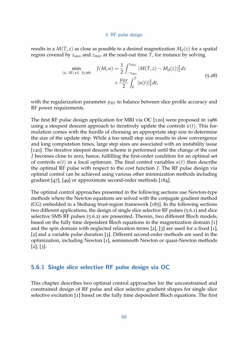
5 RF pulse design
results in a M(T, z) as close as possible to a desired magnetization Md(z) for a spatialregion covered by zmin and zmax at the read-out time T, for instance by solving
min(u, M) s.t. (5.26)
J(M, u) =12
∫ zmax
−zmin
|M(T, z)−Md(z)|22 dz
+µRF
2
∫ T
0|u(t)|22 dt,
(5.28)
with the regularization parameter µRF to balance between slice profile accuracy andRF power requirements.
The first RF pulse design application for MRI via OC [120] were proposed in 1986
using a steepest descent approach to iteratively update the controls u(t). This for-mulation comes with the hurdle of choosing an appropriate step size to determinethe size of the update step. While a too small step size results in slow convergenceand long computation times, large step sizes are associated with an instability issue[120]. The iterative steepest descent scheme is performed until the change of the costJ becomes close to zero, hence, fulfilling the first-order condition for an optimal setof controls u(t) in a local optimum. The final control variables u(t) then describethe optimal RF pulse with respect to the cost function J. The RF pulse design viaoptimal control can be achieved using various other minimization methods includinggradient [47], [49] or approximate second-order methods [184].
The optimal control approaches presented in the following sections use Newton-typemethods where the Newton equations are solved with the conjugate gradient method(CG) embedded in a Steihaug trust-region framework [185]. In the following sectionstwo different applications, the design of single slice selective RF pulses (5.6.1) and sliceselective SMS RF pulses (5.6.2) are presented. Therein, two different Bloch models,based on the fully time dependent Bloch equations in the magnetization domain [1]and the spin domain with neglected relaxation terms [2], [3] are used for a fixed [1],[2] and a variable pulse duration [3]. Different second-order methods are used in theoptimization, including Newton [1], semismooth Newton or quasi-Newton methods[2], [3].
5.6.1 Single slice selective RF pulse design via OC
This chapter describes two optimal control approaches for the unconstrained andconstrained design of RF pulse and slice selective gradient shapes for single sliceselective excitation [1] based on the fully time dependent Bloch equations. The first
60

5 RF pulse design
section contains a brief description of the unconstrained optimal control frameworkand its limitation with respect to strict hardware limitations on the RF and sliceselective gradient waveform. These limitations are included in the optimal controlframework and described in the second section.
Unconstrained joint design of RF pulse and slice selective gradient shape
First, only the real RF pulse waveform B1,x(t) is optimized. The imaginary partof the RF pulse B1,y(t) and the selective gradient shape Gs(t) are not part of theoptimization and are set to zero and to a trapezoidal shape, respectively. Therefore,the controls u(t) are equivalent to B1,x(t). The optimization consists of minimizingthe functional
min(u, M) s.t. (5.26)
J(M, u) =12
∫ zmax
zmin
|M(T, z)−Md(z)|22dz
+µRF
2
∫ T
0|B1,x(t)|22dt,
(5.29)
at the end of the excitation time t = T that is evaluated at discrete spatial points zranging from zmin to zmax.
The optimal RF shape B1,x(t) is computed by minimizing J, see Eq. 5.29. In contrastto gradient methods that compute the update
uk+1 = uk − skg(uk), (5.30)
for a step length sk and the gradient g(uk) of Eq.5.29, the application of the Newton’smethod requires an additional derivative. However, the computation of the fullHessian H(k) is in practice computationally expensive. The computation of the fullHessian can be prevented using Krylov methods such as CG that only require tocompute the Hessian action H(uk)h for a given direction h in each iteration. Thisreduces the computational effort dramatically to the cost of a gradient evaluation [1],[186]. To achieve accurate derivative information the gradient and the action of theHessian are computed using the adjoint method. This is achieved solving the forwardBloch equations, see Eq. 5.26, and adjoint (backward in time) Bloch equations
−P(t; z) = A(u(t); z)TP(t; z), 0 ≤ t < T,P(T; z) = M(T; z)−Md(z),
(5.31)
61

5 RF pulse design
with P being the solution to the adjoint Bloch equation. The gradient can be thencalculated efficiently by
g(uk)(t) = µRFu(t) +
(∫ zmax−zmin
M(t; z)A1P(t; z) dz∫ zmax−zmin
M(t; z)A2P(t; z) dz
), 0 ≤ t ≤ T, (5.32)
with
A1 :=
0 0 00 0 −γ0 γ 0
, A2 :=
0 0 −γ0 0 0γ 0 0
. (5.33)
The computation of the Hessian action H(uk)h is done accordingly by differntiatingEq. 5.32 with respect to u and h, see [1] and 9.1.2 in the Appendix. To ensure practicalapplication of the CG Newton method and to guarantee convergence from anyarbitrary initial u(t), the Newton’s method is embedded into a Steihaug CG trust-region [185] framework. This, however, does not imply the determination of theglobally optimal solution, but the convergence to a local minimum is guaranteed. Inthe Steihaug CG trust-region framework a breakdown of the CG method is handledby a trust-region step. Additional checks before the application of the update stepon curvature, step size and actual cost decrease allow us to use the CG method forminimizing a quadratic function with a trust-region radius that is adapted iteratively.The full algorithm and discretization required for numerical optimization are givenin [1] as well as in 9.1.7 and 9.1.8 in the Appendix.
As an exemplary result, the optimal RF pulse shape B1,x(t) with respect to a Gauss-filtered rectangular slice with a THK of 5 mm and a flip angle of 90 (Md(z)) isshown in Row 1 of Figure 5.10 [187]. The optimization is initialized with a zero RFpulse and has a fixed duration of 2.56 ms (τ = 10 µs). The refocusing gradient isnot part of the optimization and is fixed to half of the gradient moment of the sliceselective gradient. The spatial domain consists of 2001 equidistant discrete samplesto incorporate a distance of ±0.2 m. The Bloch simulation at the end of the gradientrefocusing is shown and compared to experimental GRE magnitude reconstructionof the measured slice profile. The choice of the regularization parameter µRF inEq. 5.29 is done with respect to the best ratio between the slice profile accuracy, RFpeak amplitude and RF power requirements. Figure 5.11 shows this for differentoptimization runs with different regularization parameters to find the best value forthe optimization of a MB6 excitation pulse used in [1] and shown in Figure 5.16.
The extension to a joint design of both the RF shape and the slice selective gradientshape is straight forward. The vector notation of the optimization enables directextension of the controls to include the slice selective gradient in the optimizationas well. Besides tracking to a desired Md this allows for reduction of the RF power
62

5 RF pulse design
x
s
s
z [m]
-0.05 0 0.05
norm
alized m
agnetization
0
1
z [m]
-0.05 0 0.05
norm
alized m
agnetization
0
1
z [m]
-0.05 0 0.05
norm
alized m
agnetization
0
1
z [m]
-0.05 0 0.05
norm
alized m
agnetization
0
1
position in mm
-50 0 50
norm
alized s
ignal [a
.u.]
0
position in mm
-50 0 50
norm
alized s
ignal [a
.u.]
0
position in mm
-50 0 50
norm
alized s
ignal [a
.u.]
0
position in mm
-50 0 50
norm
alized s
ignal [a
.u.]
0
A A B B
AB
x
s
s
Figure 5.10: RF only (Row 1) and joint RF/Gs (Row 2) optimization (left) together with the simulated(middle) and measured transverse magnetization (right). Row 3 shows the experimentalphantom an in vivo magnitude reconstructions using the RF and gradient shapes RF only(A) and joint RF/Gs (B) [187].
63

5 RF pulse design
µRF µRF µRF
10-6 10-4 10-2no
rma
lize
d r
ela
tive
err
or
0.06
0.065
0.07
0.075
0.08
10-6 10-4 10-2 R
F e
ne
rgy
80
100
120
140
10-6 10-4 10-2
ma
x B
1
10
11
12
13
Figure 5.11: Optimized SMS pulses with different regularization parameter µRF. The relative erroris defined as the normalized point-wise Euclidean norm ||M − Md||22/||Md||22 and theaverage RF energy is ||B1||22. The red circle depicts the µRF used in [1].
requirements of the RF pulse by changing the k-space velocity, a similar effect asdescribed in Section 5.4 (VERSE). However, the slice selective gradient is changedhere in each iteration simultaneously with the RF pulse.
The optimization results for a joint optimization of RF and slice selective gradient isdepicted in Row 2 of Figure 5.10. Again, the optimization is started with a zero RFpulse and the trapezoidal slice selective gradient with respect to the same parametersas stated above. Now, the first 256 samples of the slice selective gradient are modifiedin the optimization, thus leading to simultaneous reduction and stretching of both,the RF and slice selective gradient shape to reduce the RF power present in the costfunction Eq. 5.29. This reduces the RF power by 30% with only a low increase of themean squared error (0.26% to 0.31%). The peak slew rate of the optimized gradient(120 T m−1 s−1) remains below the prescribed maximal rate (180 T m−1 s−1) of theused system. It should be noted, however, that the optimization is unconstrained anddepending on the regularization parameters the optimized waveforms may violateMR scanner hardware limits. An experimental comparison of the two optimizedresults is depicted in Row 3 of Figure 5.10 for a standard GRE in vivo scan and amodified GRE phantom scan to directly measure the slice profile, see Section 4.2.The intersection line depicts the position of the profile. The joint design yieldssharp slice profiles and reduced RF power requirements without the need of explicitpower reduction techniques such as VERSE [112], see Section 5.4. The matrix-freeimplementation allows computation of a larger number of temporal and spatialcontrol points compared to the gVERSE [188] approach that is limited with 15 spatialpoints. Depending on the regularization parameters it is possible to compute pulseswith an even lower SAR depending on hardware limitations, in particular the gradientslew rate.
64

5 RF pulse design
Constrained joint design of RF pulse and slice selective gradient shape
The design approach described before enables an unconstrained optimization ofboth the RF pulse and slice gradient shape at a high spatial and temporal resolution[1]. However, the optimized results could exceed physical constraints and thereforemay not be realized on a real MR scanner. To include hard constraints of actualMR hardware, the previously introduced framework is extended to a trust-regionsemismooth Newton method to include physical constraints such as the peak B1amplitude of the RF pulse and the slew rate of the gradient system [2].
The optimization is again based on minimizing the difference between the forwardBloch simulation at the end of the pulse duration M(T, z) and the desired magneti-zation Md(z). Three additional cost terms model the power of the RF pulse B1,x, theslew rate Gs and the final amplitude of Gs
min(u, M) s.t. (5.26)
J(M, u) =12
∫ z
−z|M(T; z)−Md(z)|22 dz +
µRF
2
∫ T
0|B1,x(t)|22 dt
+µGs
2
∫ T
0|Gs(t)|22 dt +
µs
2|Gs(T)|22,
(5.34)
with the regularization parameters µRF, µGs , µs. To include peak RF and slew rateamplitude constraints, these are added as point-wise inequality constraints on thecontrol variables u(t):
|B1|∞ ≤ B1,max and |Gs|∞ ≤ Gs,max. (5.35)
Now, the Newton method is not applicable any longer due to a resulting set ofnonsmooth equations [2]. However, such problems can be efficiently solved with gen-eralized semismooth Newton methods [190] based on projections without increasingthe computational effort. The semismooth Newton-derivative can be evaluated forthe Hessian action similar to the unconstrained design [1]. In addition to the efficientapplication, semismooth Newton methods converge locally superlinear which makesthem an highly efficient method for OC problems with inequality constraints [2].Again, the gradient and Hessian information are computed with the adjoint calcu-lus. The generalized semismooth Newton method is embedded in a Steihaug CGtrust-region framework [185], [191].
Figure 5.12 compares a conventional Hamming filtered SINC pulse with the resultsof the unconstrained optimization together with the constrained optimization (peakRF magnitude B1,max = 13 µT, peak slew rate Gs = 175 mT m−1 s−1) [189]. The Blochsimulations show a well-defined slice profile for all three examples. However, only
65

5 RF pulse design
conventional
0 0.5 1
20
10
0
10
20
30
40
t [ms]
B1
[µT
], G
s[m
T/m
]
B1,x
B1,y
Gs
0.05 0 0.05
0
1
z [m]
no
rma
lize
d m
ag
ne
tiza
tio
n
|Mxy
(T)|
|Mi,xy
|
0.05 0 0.05
0
1
z [m]
no
rma
lize
d m
ag
ne
tiza
tio
n
0.01 0.005 0 0.005 0.01
z [m]
ph
ase
[ra
d] i
0.01 0.005 0 0.005 0.01
-
z [m]
ph
ase
[ra
d]
unconstrained
0 0.5 1
20
10
0
10
20
30
40
t [ms]
B1
[µT
], G
s[m
T/m
]
B1,x
B1,y
Gs
0.05 0 0.05
0
1
z [m]
no
rma
lize
d m
ag
ne
tiza
tio
n
|Mxy
(T)|
|Mi,xy
|
0.05 0 0.05
0
1
z [m]
no
rma
lize
d m
ag
ne
tiza
tio
n
0.01 0.005 0 0.005 0.01z [m]
ph
ase
[ra
d] i
0.01 0.005 0 0.005 0.01
-
z [m]
ph
ase
[ra
d]
constrained
0 0.5 1
20
10
0
10
20
30
40
t [ms]
B1
[µT
], G
s[m
T/m
]
B1,x
B1,y
Gs
0.05 0 0.05
0
1
z [m]
no
rma
lize
d m
ag
ne
tiza
tio
n
|Mxy
(T)|
|Mi,xy
|
0.05 0 0.05
0
1
z [m]
no
rma
lize
d m
ag
ne
tiza
tio
n
0.01 0.005 0 0.005 0.01z [m]
ph
ase
[ra
d] i
0.01 0.005 0 0.005 0.01
-
z [m]
ph
ase
[ra
d]
θ
θ
θ
θ
θ
θ
Figure 5.12: Conventional Hamming window filtered SINC with standard trapezoidal gradient slope,low SAR optimized unconstrained and constrained RF and Gs shapes (both with µRF =5e − 4, µGs = 3e − 4, µs = 1.25), second line: simulated (Mxy) and ideal transversemagnetization (Mi,xy), third line: simulated and ideal phase (θ and θd) [189].
66
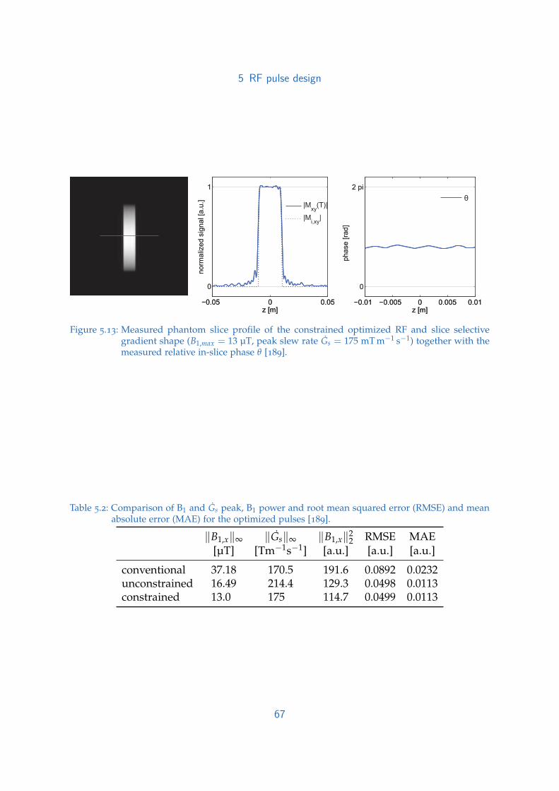
5 RF pulse design
−0.05 0 0.05
0
1
z [m]
no
rma
lize
d s
igna
l [a
.u.]
|Mxy
(T)|
|Mi,xy
|
−0.05 0 0.05
0
1
z [m]
no
rma
lize
d s
igna
l [a
.u.]
−0.01 −0.005 0 0.005 0.01
0
2 pi
z [m]
ph
ase [
rad]
−0.01 −0.005 0 0.005 0.01
0
2 pi
z [m]
pha
se
[ra
d]
θ
Figure 5.13: Measured phantom slice profile of the constrained optimized RF and slice selectivegradient shape (B1,max = 13 µT, peak slew rate Gs = 175 mT m−1 s−1) together with themeasured relative in-slice phase θ [189].
Table 5.2: Comparison of B1 and Gs peak, B1 power and root mean squared error (RMSE) and meanabsolute error (MAE) for the optimized pulses [189].
‖B1,x‖∞ ‖Gs‖∞ ‖B1,x‖22 RMSE MAE
[µT] [Tm−1s−1] [a.u.] [a.u.] [a.u.]
conventional 37.18 170.5 191.6 0.0892 0.0232unconstrained 16.49 214.4 129.3 0.0498 0.0113constrained 13.0 175 114.7 0.0499 0.0113
67

5 RF pulse design
−0.01 −0.005 0 0.005 0.01
0
1
z [m]
no
rma
lize
d m
ag
ne
tiza
tio
n Md,x
Md,y
Md,z
−0.01 −0.005 0 0.005 0.01
0
1
z [m]
no
rma
lize
d m
ag
ne
tiza
tio
n
−0.1 −0.05 0 0.05 0.1
−1
0
1
z [m]
no
rma
lize
d m
ag
ne
tiza
tio
n
Md,x
Md,y
Md,z
−0.1 −0.05 0 0.05 0.1
−1
0
1
z [m]
no
rma
lize
d m
ag
ne
tiza
tio
n−0.1 −0.05 0 0.05 0.1
−1
0
1
z [m]
no
rma
lize
d m
ag
ne
tiza
tio
n
Md,x
Md,y
Md,z
−0.1 −0.05 0 0.05 0.1
−1
0
1
z [m]
no
rma
lize
d m
ag
ne
tiza
tio
n
Figure 5.14: Desired magnetization Md for single (a) and SMS design with 6 slices with different phasepatterns (b,c) [1].
the constrained results are directly applicable on the MR scanner. The unconstrainedresults violate the hardware limitations and have to be stretched in time to reducepeak RF and slew rate of the slice selective gradient. The numerical simulationsare validated by magnitude and phase images of experimental 3 T phantom mea-surements in Figure 5.13. The significant key features are summarized in Table 5.2.Despite using a constrained optimization, the optimized pulses achieve a similarslice profile compared to the unconstrained optimization while having the benefit ofguaranteed practical applicability.
5.6.2 SMS RF pulse design via OC
The OC based design method introduced in the previous Section 5.6.1 can be easilyextended to the design of SMS pulses and gradient shapes. For this purpose, thedesired magnetization is changed to contain more than one slice, for instance sixequidistant slices, as shown in Figure 5.14. The following sections describe theunconstrained and constrained design of SMS RF pulses with fixed pulse durationand optimized pulse duration.
Unconstrained SMS excitation
The unconstrained OC approach to design SMS RF pulse shapes is done in a similarway to Section 5.6.1 and consists of minimizing the discrepancy between the numericalsolution of the fully time-dependent Bloch equations and a prescribed magnetizationprofile together with a cost term modeling the pulse power, see Eq. 5.29. The useof different desired magnetization patterns, see Figure 5.14, now results in SMS RF
68

5 RF pulse design
time in ms
simulation experiment
B1 in
µT
an
d G
s in
mT
/m
B1,x
B1,y
Gs
-10
-5
0
5
10
distance in m
norm
aliz
ed m
agnetiz
atio
n0
0.5
1
distance in m
magnitude in a
.u.
-0.05 0 0.050 2 4 6 8 -0.05 0 0.05
Figure 5.15: Optimized SMS RF pulse for three slices with different flip angles (φ = (65, 35, 15) ) andexperimental phantom reconstruction [193].
pulses. The source code used to generate the examples can be downloaded fromhttps://github.com/chaigner/rfcontrol/releases/v1.2 [1].
This approach was applied to compute RF pulses for a simultaneous excitation, con-sidering a z-range of 400 mm with a spatial resolution of 0.02 mm and a thickness of5 mm for each slice. The high spatial resolution is important to suppress a modulationof the magnetization. The pulses were designed for a total excitation time T = 2.56ms and consisted of 256 samples. For each slice, a flip angle of 25 [192] or 90 wasspecified [1], see also Figure 5.14. Alternatively, the OC-based design approach allowsfor the choice of any arbitrary desired magnetization pattern, for instance choosingdifferent flip angles for individual slices [193]. This is exemplary shown in Figure 5.15
for an optimized complex SMS excitation pulse to excite three slices with differentflip angles (φi = (65, 35, 15) ). The numerical results are imported to the previouslydescribed GRE sequence to perform phantom and in vivo measurements.
Figure 5.16 shows optimized RF pulses (B1,x, B1,y) together with the prescribed sliceselective gradient Gs, the corresponding simulated slice profiles and the centralline of the reconstructed phantom magnitude images for a flip angle of 90 . Toseparate aliased slice information in the case of in vivo imaging, we use the slice-GRAPPA (sG) algorithm [172] with reference scans of 24 phase encoding lines perslice. Since the reconstruction starts to suffer from g-factor problems for more thanthree slices, we modified the above-described SMS pulses using a CAIPIRINHA-basedexcitation pattern [171], which alternates two different pulses to achieve phase-shiftedmagnetization vectors in order to increase the spatial distance of aliased voxels bya factor of FOV/2 for every second slice. As it can be seen in Row 2 of Figure 5.16,the optimized pulses lead to the desired excitation pattern while the remainingcolumns show the sG reconstructions, which illustrate the uniform excitation and theapplicability of the optimized pulses for in vivo experiments.
69

5 RF pulse design
slice GRAPPA reconstruction
slice 1 slice 2 slice 3 slice 4 slice 5 slice 6
0 5 1015
0
15
time [ms]
B1
[µT
], G
z[m
T/m
]
B1,x
B1,y
Gs
optimized pulse
0.05 0 0.050
0.5
1
z [m]
no
rma
lize
d m
ag
ne
tiza
tio
n
0.05 0 0.050
0.5
1
z [m]
no
rma
lize
d m
ag
ne
tiza
tio
n
optimized slice profile
0.05 0 0.050
500
1000
1500
2000
position in m
sig
na
l [a
.u.]
measured slice profile p
ha
nto
m
in v
ivo
z readout
Figure 5.16: Optimized RF pulse for six slice profiles, each with a flip angle of 90 together withsimulated magnetization patterns and experimental phantom measurements (Row 1).Cartesian and slice-GRAPPA reconstruction using CAIPIRINHA-based SMS excitation(Row 2) [1].
The simulation and optimization of the full time dependent Bloch equations withthe Crank–Nicolson method [1] turned out to introduce numerical errors [71] thatwere not visible in the numerical simulations and experimental validation. This errorincreases for off-resonant positions and leads to a slice shift and dephasing. Thisnumerical errors can be effectively reduced by increasing the temporal discretiza-tion. Figure 5.17 shows two optimization runs for six slices and compares forwardsimulations with the Crank–Nicolson method and spin domain Bloch simulations.The differences in the transversal magnetization are minimized by the finer temporaldiscretization in Row 2. A more extensive analysis of different numerical methods tosolve the Bloch equations with and without relaxation times is covered in [68].
70

5 RF pulse designd
iscre
tiza
tio
n 2
.5µ
s
dis
cre
tiza
tio
n 1
0µ
s
time in ms
0 5 10
B1 in
µT,
Gs
in m
T/m
-20
-10
0
10
20
distance in m
-0.1 0 0.1
no
rma
lize
d m
ag
ne
tiza
tio
n
0
0.5
1
distance in m
0.055 0.06 0.065 0.07
no
rma
lize
d m
ag
ne
tiza
tio
n
0
0.5
1
time in ms
0 5 10
B1 in
µT,
Gs
in m
T/m
-20
-10
0
10
20
distance in m
-0.1 0 0.1
no
rma
lize
d m
ag
ne
tiza
tio
n
0
0.5
1
distance in m
0.055 0.06 0.065 0.07
no
rma
lize
d m
ag
ne
tiza
tio
n
0
0.5
1
B1,x
B1,y
Gs
CNSD
CNSD
Figure 5.17: Optimized SMS excitation pulses using the numerical Bloch Crank–Nicolson (CN) modelwith different temporal sampling (Row 1: τ = 10 µs and Row 2: τ = 2.5 µs) together withsimulated transverse magnetization using Crank–Nicolson and spin domain (SD) Blochequations.
Constrained SMS refocusing
The joint design of RF and slice selective gradient shape via OC [1] can be extendedto the spin domain Bloch equations using the Cayley-Klein parameters a, b [2]
am = αmam−1 − β∗mbm−1,bm = βmam−1 + α∗mbm−1,
(5.36)
and α, β defined in Eq. 3.15 together with the initial conditions a0 = 1, b0 = 0.The controls x are the complex RF pulse B1,m = rmexp(iϑm) and the slice selectivegradient slew rate sm = gm − gm−1/τ for each discrete time point m. Contrary to thepreviously described design of single and SMS excitation pulses, SMS refocusingpulses are designed in the spin domain assuming perfect crusher gradients. Therefore,the desired refocusing profile (magnitude and phase) at the end of the refocusingtime T is defined in-slice as 1− |β(z)|2 ≤ ein, out-of-slice as |β(z)|2 ≤ eout togetherwith a in-slice phase constraint |ϕ− ϕ| ≤ eph with the phase ϕ and desired mean
71

5 RF pulse design
phase ϕ based on the parameter relations in [66] and Tab. 5.1. The optimization isdone to minimize the RF energy requirements by minimizing the functional
min(x) s.t. (5.36)
J =τ
2
Nt
∑m=1
r2m + ζϑ2
m + ζg2m
+δµout
2p ∑zj∈Ωout
(|bNt |2
e
)p
+δµin
2p ∑zj∈Ωin
(|bNt |2 − 1
e
)p
+δµp
p
L
∑l=1
∑zj∈Sl
(ϕ− ϕl
ep
)p+
τµg
p
Nt
∑m=2
(gm − gm−1
τsmax
)p,
where x are the control variables, p is an even positive integer, rm the RF amplitude,ϑm the RF phase, gm the slice selective gradient and ζ, µout, µin, µp and µg being theregularization parameters. The regularization parameters are initialized with ζ = 0.01,µout = 1e5, µin = 1e4, µp = 1 and µg = 1. To balance between the different terms theregularization parameters are being adapted throughout the optimization [2]. Hardamplitude constraints on the RF amplitude (0 ≤ r ≤ B1,max), RF phase (−π ≤ ϑ ≤ π)and slew rate of the slice selective gradient (−smax ≤ gm − gm−1 ≤ smax) are includedfor the controls. The resulting set of nonsmooth equations are solved for a fixed pby a semismooth quasi-Newton method [190] that is embedded in a Steihaug CGtrust-region framework [185], [191]. Throughout the optimization, the parameter pis successively increased starting with a small number, for instance p = 2, until theminimum pulse energy is found. For a full description refer to [2], or 9.2.2, 9.2.3 and9.2.7 in the Appendix.
The proposed algorithm is tested to reduce the power requirements of different SMSpulses including superposition, PINS and root flipping as well as examples given bythe ISMRM Challenge 2015 test set [83] for a fixed pulse duration [2]. To guaranteepractical applicability on the MR system used, the time discretization is fixed to agradient raster time of τ = 10 µs. Throughout the optimization, the parameter p isiteratively increased with a decrease of all µ in Eq. 5.37 to find a minimal RF powersolution. Figure 5.18 shows an optimized result for SMS refocusing with a MB factorof 6, a THK of 1.75 mm and a TBWP of 4 starting from a root flipping [173] initialfor peak RF amplitude B1,max = 13 µT, a peak slew rate Gs,max = 200 T m−1 s−1,and a maximum refocusing error of 5% (in-slice) and 4% (out-slice). The phase ofthe refocusing profiles was not included since root flipping pulses do not have alinear phase profile [173]. Other optimized results are presented in [2] and in 9.2.4 ofthe Appendix. Optimized SMS pulses with a MB factor of 3 and 10 respectively areimplemented on a 3 T MR scanner (Magnetom Skyra, Siemens Healthcare, Erlangen,Germany) using a spin echo sequence with a conventional superposed 90 SLRbased SMS excitation pulse. These results are depicted in Figure 5.19 for phantom
72

5 RF pulse design
time in ms
0 2 4 6 8B1 in
µT,
Gs in
mT
/m
-10
0
10
20
time in ms
0 2 4 6 8B1 in
µT,
Gs in
mT
/m
-10
0
10
20
distance in m
-0.03 -0.02 -0.01 0 0.01 0.02 0.03
refo
cu
sin
g p
rofile
0
0.5
1
distance in m
-0.03 -0.02 -0.01 0 0.01 0.02 0.03re
focu
sin
g p
rofile
0
0.5
1
distance in m
-0.022 -0.02 -0.018 -0.016 -0.014
refo
cu
sin
g p
rofile
0
0.5
1
distance in m
-0.02 -0.019 -0.018 -0.017 -0.016
ph
ase
an
gle
-2
0
2
Figure 5.18: Numerical optimization results and spin domain Bloch simulations for a MB6 pulse.Initial (Row 1) and optimized (Row 2) RF and Gs (Re(RF) in blue, Im(RF) in yellow andGs in red) with refocusing profile |bNt |2. Zoom of the central slice (black lines mark thein-slice/out-of-slice error tolerance) with phase angle(bNt) (not part of the optimization)for the optimized pulse (Row 3) [2].
and in vivo measurements (TR/TE= 100/25− 30 ms, FOV= 300× 300 mm, matrix=1536 × 1536 with 922 phase encoding steps) and an in vivo scan (TR/TE= 200/15ms, FOV= 300 × 300 mm, matrix= 512 × 512). The reconstructed high resolutionexperimental phantom data is further directly compared with the numerical results,thereby validating the Bloch simulations. Across a wide range of parameters the pulsepower is dramatically reduced. Both the phantom and in vivo measurements showwell defined slices and validate the Bloch simulations, demonstrating the ability tojointly design RF and slice selective gradient shapes with hard inequality constraints.
73
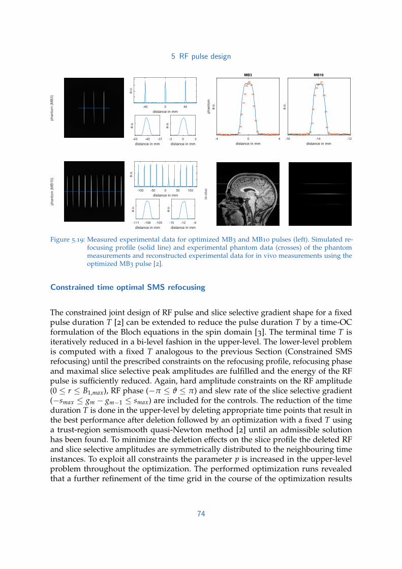
5 RF pulse designphanto
m (
MB
3)
distance in mm
-40 0 40
a.u
.
distance in mm
-3 0 3
a.u
.
distance in mm
-43 -40 -37
a.u
.
phanto
m (
MB
10)
distance in mm
-100 -50 0 50 100
a.u
.
distance in mm
-15 -12 -9
a.u
.
distance in mm
-111 -108 -105
a.u
.
in-v
ivo
distance in mm
-4 0 4
a.u
.
MB3
distance in mm
-16 -14 -12
a.u
.
MB10
phanto
m
Figure 5.19: Measured experimental data for optimized MB3 and MB10 pulses (left). Simulated re-focusing profile (solid line) and experimental phantom data (crosses) of the phantommeasurements and reconstructed experimental data for in vivo measurements using theoptimized MB3 pulse [2].
Constrained time optimal SMS refocusing
The constrained joint design of RF pulse and slice selective gradient shape for a fixedpulse duration T [2] can be extended to reduce the pulse duration T by a time-OCformulation of the Bloch equations in the spin domain [3]. The terminal time T isiteratively reduced in a bi-level fashion in the upper-level. The lower-level problemis computed with a fixed T analogous to the previous Section (Constrained SMSrefocusing) until the prescribed constraints on the refocusing profile, refocusing phaseand maximal slice selective peak amplitudes are fulfilled and the energy of the RFpulse is sufficiently reduced. Again, hard amplitude constraints on the RF amplitude(0 ≤ r ≤ B1,max), RF phase (−π ≤ ϑ ≤ π) and slew rate of the slice selective gradient(−smax ≤ gm − gm−1 ≤ smax) are included for the controls. The reduction of the timeduration T is done in the upper-level by deleting appropriate time points that result inthe best performance after deletion followed by an optimization with a fixed T usinga trust-region semismooth quasi-Newton method [2] until an admissible solutionhas been found. To minimize the deletion effects on the slice profile the deleted RFand slice selective amplitudes are symmetrically distributed to the neighbouring timeinstances. To exploit all constraints the parameter p is increased in the upper-levelproblem throughout the optimization. The performed optimization runs revealedthat a further refinement of the time grid in the course of the optimization results
74

5 RF pulse design
in even shorter pulse durations. The refinement, however, has to be used withcare with respect to gradient raster time of the MR system. For a full descriptionrefer to [3], or 9.3.2 in the Appendix. The source code can be downloaded fromhttps://github.com/rundar/mr.control.
To test the general applicability of the proposed design method, we minimizedthe pulse duration in the test set of 31 cases from the 2015 ISMRM pulse designchallenge [83]. The iterative optimization was initialized with PINS [131]-based RFand triangular slice selective gradient shapes with respect to a B1,max = 18 µT, andGs,max = 200 T m−1 s−1, and a maximum refocusing error of 3% and 2% for in-and out-slice regions respectively. A representative optimized TSE result (MB= 12,TBWP= 3, THK= 1 mm) is depicted in Figure 5.20. The exploitation of the hardwareconstraints, see Row 1 of Figure 5.20, and a p driven to large even numbers, allowedfor determination of the shown result with a pulse duration T reduced by 75% from12.92 ms to 3.16 ms compared to the initial PINS pulse that still fulfils all controlconstraints. An overview of all optimized 31 examples of the ISMRM challenge [83]
Table 5.3: Comparison of the optimized pulse duration (in ms) with the duration of the PINS initialguess for all examples without constraints on the refocusing phase.
MB3 MB4 MB5
THK PINS opt PINS opt PINS optmm ms ms ms ms ms ms
2.00 16.870 2.155 15.090 2.285 13.560 2.414
1.75 18.460 2.155 16.400 2.448 14.140 2.502
1.50 21.260 2.336 18.470 2.539 16.090 2.651
1.25 24.370 2.470 21.180 2.673 18.320 2.404
1.00 28.840 2.650 25.250 2.805 21.180 2.938
is summarized in Tables 5.3 and 5.4 and compare the time optimal pulse durationwith the used PINS initial guesses. The optimized slice selective gradient resulted ina varying k-space trajectory that makes the pulse possibly prone to B0 off-resonanceinfluences and B1 inhomogeneities. Figure 5.21 shows Bloch simulations with aconstant global B0 off-resonance variation of ±200 Hz and B1 variation of 75%-125%with stable slice profiles below ±100 Hz. To validate the numerical results, theoptimized pulses were computed for the gradient raster time of τ = 10 µs, whichresults in a pulse duration of T = 3.3 ms on the 3 T MR scanner (Magnetom Skyra,Siemens Healthcare, Erlangen, Germany) used and imported to a spin echo sequence.Phantom experiments were performed with a conventional SLR based 90 SMSexcitation pulse acquiring high-resolution phantom scans (TR/TE = 300/30 ms,FOV = 300 × 300 mm, matrix = 960 × 960) where the phase encoding is applied inslice-direction. The experimental results are shown in Figure 5.22. To validate the
75

5 RF pulse design
time in ms
0 0.5 1 1.5 2 2.5 3
Gs
in m
T/m
0
20
40
60
time in ms
0 0.5 1 1.5 2 2.5 3
RF
in µ
T
-20
-10
0
10
20
time in ms
0 0.5 1 1.5 2 2.5 3
sle
w r
ate
in T
/m/s
-200
-100
0
100
200
distance in mm
-100 -50 0 50 100re
focusin
g p
rofile
0
0.5
1
distance in mm
-12 -10 -8
refo
cu
sin
g p
rofile
0
0.5
1
-110
an
gle
-2
0
2
-90 -70 -50 -30
distance in mm
-10 10 30 50 70 90 110
Figure 5.20: Optimization results and Bloch simulations for one representative TSE example. The firstrow shows the control variables B1 amplitude and slew rate of the slice selective gradientfor the refocusing duration of T = 3.16 ms. The second row depicts the slice selectivegradient shape, and the corresponding simulated refocusing profile |bNt |2. The last rowshows a detail zoom of one slice to see the refocusing profile together with the errorcorridor (black), and the phase angle arg(b2
Nt) per slice [3].
Table 5.4: Comparison of the optimized pulse duration (in ms) with the duration of the PINS initialguess for all TSE examples.
MB8 MB10 MB12 MB14
THK PINS opt PINS opt PINS opt PINS optmm ms ms ms ms ms ms ms ms
2.0 10.640 2.742 9.460 2.856 8.810 2.728 8.710 2.809
1.5 13.260 3.295 11.110 3.213 10.890 3.286 10.300 3.296
1.0 18.040 3.958 15.170 4.122 14.460 4.120 14.110 3.996
0.5 32.420 6.106 27.390 6.113 25.230 6.080 24.520 6.189
76
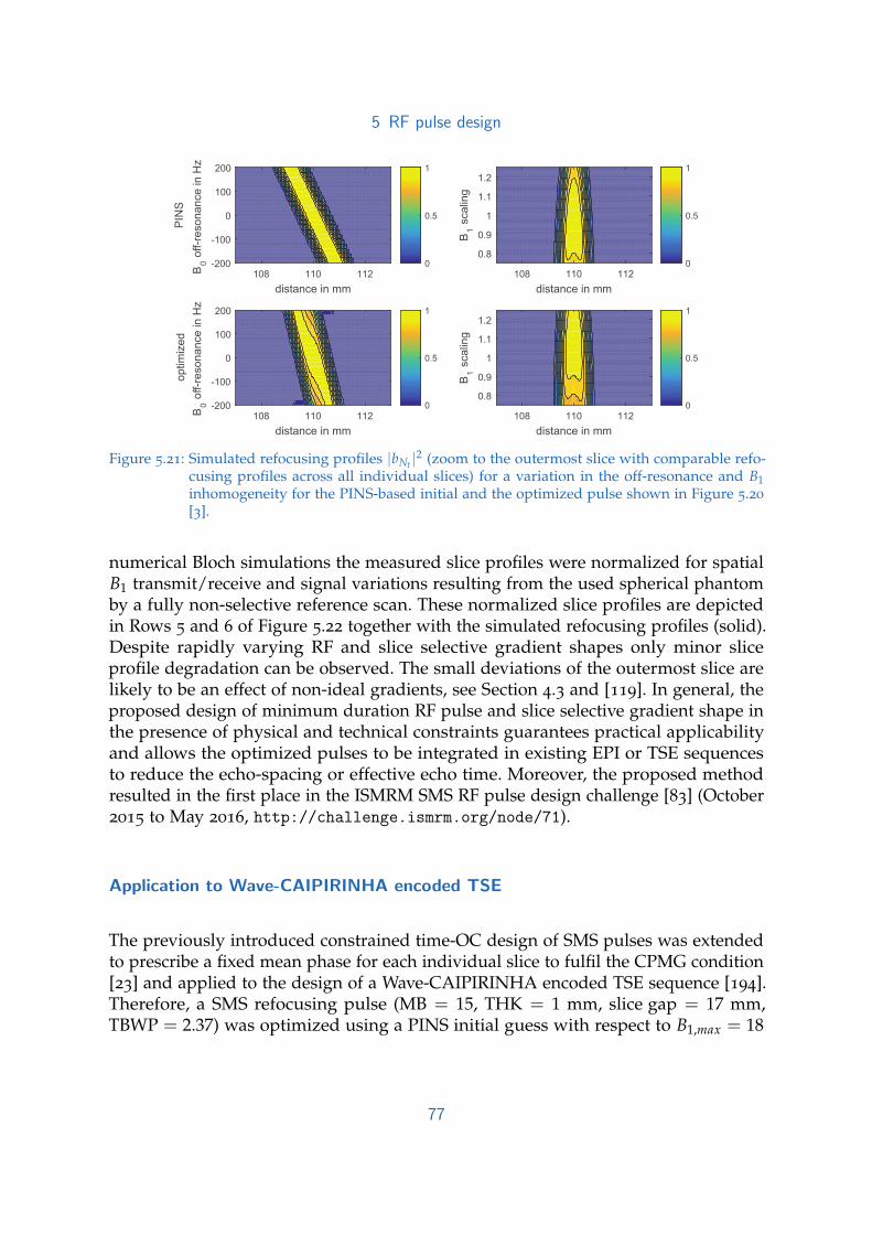
5 RF pulse design
distance in mm
108 110 112
B1
scalin
g
0.8
0.9
1
1.1
1.2
0
0.5
1
distance in mm
108 110 112B0
off-r
eso
nance in H
z
-200
-100
0
100
200
0
0.5
1
distance in mm
108 110 112
B1
scalin
g
0.8
0.9
1
1.1
1.2
0
0.5
1
distance in mm
108 110 112B0
off-r
eso
nance in H
z
-200
-100
0
100
200
0
0.5
1
optim
ized
PIN
S
Figure 5.21: Simulated refocusing profiles |bNt |2 (zoom to the outermost slice with comparable refo-cusing profiles across all individual slices) for a variation in the off-resonance and B1inhomogeneity for the PINS-based initial and the optimized pulse shown in Figure 5.20
[3].
numerical Bloch simulations the measured slice profiles were normalized for spatialB1 transmit/receive and signal variations resulting from the used spherical phantomby a fully non-selective reference scan. These normalized slice profiles are depictedin Rows 5 and 6 of Figure 5.22 together with the simulated refocusing profiles (solid).Despite rapidly varying RF and slice selective gradient shapes only minor sliceprofile degradation can be observed. The small deviations of the outermost slice arelikely to be an effect of non-ideal gradients, see Section 4.3 and [119]. In general, theproposed design of minimum duration RF pulse and slice selective gradient shape inthe presence of physical and technical constraints guarantees practical applicabilityand allows the optimized pulses to be integrated in existing EPI or TSE sequencesto reduce the echo-spacing or effective echo time. Moreover, the proposed methodresulted in the first place in the ISMRM SMS RF pulse design challenge [83] (October2015 to May 2016, http://challenge.ismrm.org/node/71).
Application to Wave-CAIPIRINHA encoded TSE
The previously introduced constrained time-OC design of SMS pulses was extendedto prescribe a fixed mean phase for each individual slice to fulfil the CPMG condition[23] and applied to the design of a Wave-CAIPIRINHA encoded TSE sequence [194].Therefore, a SMS refocusing pulse (MB = 15, THK = 1 mm, slice gap = 17 mm,TBWP = 2.37) was optimized using a PINS initial guess with respect to B1,max = 18
77
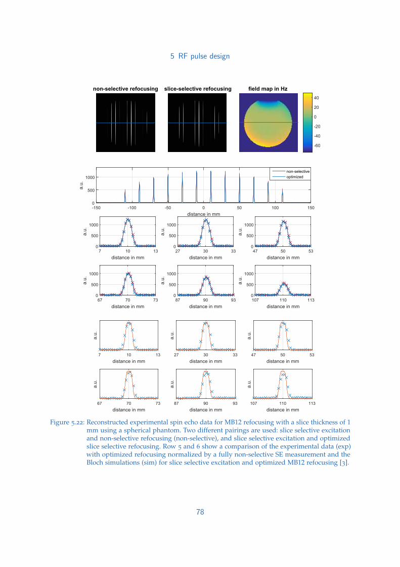
5 RF pulse design
non-selective refocusing slice-selective refocusing field map in Hz
-60
-40
-20
0
20
40
distance in mm
-150 -100 -50 0 50 100 150
a.u
.
0
500
1000
non-selective
optimized
distance in mm
7 10 13
a.u
.
0
500
1000
distance in mm
27 30 33
a.u
.
0
500
1000
distance in mm
47 50 53
a.u
.
0
500
1000
distance in mm
67 70 73
a.u
.
0
500
1000
distance in mm
87 90 93
a.u
.
0
500
1000
distance in mm
107 110 113
a.u
.
0
500
1000
distance in mm
7 10 13
a.u
.
distance in mm
27 30 33
a.u
.
distance in mm
47 50 53
a.u
.
distance in mm
67 70 73
a.u
.
distance in mm
87 90 93
a.u
.
distance in mm
107 110 113
a.u
.
Figure 5.22: Reconstructed experimental spin echo data for MB12 refocusing with a slice thickness of 1mm using a spherical phantom. Two different pairings are used: slice selective excitationand non-selective refocusing (non-selective), and slice selective excitation and optimizedslice selective refocusing. Row 5 and 6 show a comparison of the experimental data (exp)with optimized refocusing normalized by a fully non-selective SE measurement and theBloch simulations (sim) for slice selective excitation and optimized MB12 refocusing [3].
78
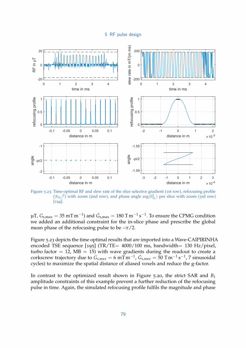
5 RF pulse design
time in ms
0 1 2 3 4
RF
in
µT
-20
0
20
time in ms
0 1 2 3 4sle
w r
ate
in
mT
/(m
ms)
-200
0
200
distance in m
-0.1 -0.05 0 0.05 0.1
refo
cu
sin
g p
rofile
0
0.5
1
distance in m ×10-3
-2 -1 0 1 2re
focu
sin
g p
rofile
0
0.5
1
distance in m
-0.1 -0.05 0 0.05 0.1
an
gle
-2
-pi/2
-1
distance in m ×10-4
-3 -2 -1 0 1 2 3
an
gle
-1.59
-pi/2
-1.55
Figure 5.23: Time-optimal RF and slew rate of the slice selective gradient (1st row), refocusing profile(|bNt |2) with zoom (2nd row), and phase angle arg(b2
Nt) per slice with zoom (3rd row)
[194].
µT, Gs,max = 35 mT m−1) and Gs,max = 180 T m−1 s−1. To ensure the CPMG conditionwe added an additional constraint for the in-slice phase and prescribe the globalmean phase of the refocusing pulse to be –π/2.
Figure 5.23 depicts the time optimal results that are imported into a Wave-CAIPIRINHAencoded TSE sequence [195] (TR/TE= 4000/100 ms, bandwidth= 130 Hz/pixel,turbo factor = 12, MB = 15) with wave gradients during the readout to create acorkscrew trajectory due to Gs,max = 6 mT m−1, Gs,max = 50 T m−1 s−1, 7 sinusoidalcycles) to maximize the spatial distance of aliased voxels and reduce the g-factor.
In contrast to the optimized result shown in Figure 5.20, the strict SAR and B1amplitude constraints of this example prevent a further reduction of the refocusingpulse in time. Again, the simulated refocusing profile fulfils the magnitude and phase
79

5 RF pulse design
Figure 5.24: Phantom (Row 1) and in vivo (Row 2) RARE/TSE measurement using the optimizedpulse shown in Figure 5.23 after Wave-CAIPIRINHA reconstruction [194].
constraints in the observed slice regions. Measurements are performed on a 3 T MRScanner (Magnetom Trio, Siemens Healthcare, Erlangen, Germany) for a phantomand in vivo. The Wave-CAIPIRINHA reconstruction of the optimized RF pulse isshown in Figure 5.24 for a phantom (Row 1) and in vivo (Row 2). The optimized RFpulse and slice selective gradient fulfil the hard constraints given by actual scannerhardware and safety measures that ensures a simple replacement of existing pulsesand is well suited to further decrease the echo spacing in TSE/RARE sequences. Thecombination of optimized pulses for large MB factors with a Wave-CAIPIRINHAreconstruction allows for fast acquisition of whole head TSE/RARE imaging in 70 s.
80

6 Discussion
This thesis presents different methods to design RF pulse and slice selective gradientshapes. The focus was placed on single slice and SMS applications with and withoutexplicit hardware constraints for the full Bloch equations including relaxation effectsand the spin domain Bloch equations with neglected relaxation terms. A summariseddiscussion of the key results is presented below.
Compared to standard RF design methods, OC approaches are flexible in the problemformulation and can be modified to prescribe various problem parameters rangingfrom a point-wise description of the desired magnetization [1] to maximal error andamplitude bounds on the state and control variables [2]. The theory is described forboth, the full [1] and the spin domain Bloch equations [2], [3], while most of theoptimization runs are done with neglected relaxation times. For standard in vivoimaging of the human head, this is a valid assumption since the relaxation times arevery long compared to the RF pulse duration. Nevertheless, the inclusion of relaxationtimes is possible using the design approach based on the full time dependent Blochequations [1]. More details on the theory and the employed methods can be found inthe Appendix.
The increased computational effort of numerical optimization is kept low by anefficient computation of exact or approximate second order information to speed upconvergence and by using a trust region framework for robustness and numericalefficiency. Large numbers of spatial points are efficiently computed by means of GPUor CPU parallelization. The RF and slice selective gradient shapes are treated in theoptimization as piecewise constant functions. This form of modelling reflects howexternal fields are implemented in MR sequences.
The performed studies show that the OC based design of RF pulse shapes increasesthe slice profile accuracy without major RF power reduction [1]. The RF powerrequirements can be reduced, however, by a joint design of RF and slice selectivegradient waveforms [2]. This is in good accordance with the VERSE theory and comeswith the benefits of a constant raster time and single step formulation, rather thansplitting the design of RF and slice selective gradient. Therefore, jointly optimizedRF and slice selective gradient shapes do not have to be interpolated to match the
81

6 Discussion
raster time, which saves interpolation errors. Additionally, the joint optimization doesnot require a scaling function and the balance between slice profile accuracy andRF power requirements can be adjusted with the regularization parameters. Theseobservations can be transferred to SMS pulse design where RF amplitude, power andduration are highly limited parameters [1].
The Crank–Nicolson scheme used to discretize the Bloch equations [1] showed slightslice profile differences as a function of the spatial position that remained undetectedby the initial experimental validation [71]. Compared to the Bloch solution withrotation matrices, off resonant spatial positions experienced a slice shift and de-phasing. Spins close to the isocenter, however, are affected by a much smaller content.It seems, that the precession of spins far away from the isocenter becomes too largefor an adequate solution by the Crank-Nicolson method. This inaccurracy can beeffectively reduced choosing finer temporal discretization as shown exemplarly byFigure 5.17. However, the optimization framework and methods are independentof the chosen Bloch solver, and hence can be extended easily to more expensiveand accurate Bloch solvers, for instance to symmetric operator splitting or piecewiseconstant analytic solution, which was done in [68]. Alternatively, the spin domainformulation can be used to accurately solve the Bloch equations with neglectedrelaxation terms [2]. The decreased computational effort compared to a numericalsolution allows looping of the optimization to address new issues, for instance areduction of the overall pulse duration [3].
While the proposed optimal control approaches use highly efficient numerical meth-ods, the computational effort is significantly greater than, for instance, SLR-basedapproaches. The optimized examples are therefore computed offline within in theminute to hour range [1]–[3] using parallel CPU computing. A proof-of-conceptGPU implementation indicates that this gap can be sufficiently narrowed to makepatient-specific design feasible [1].
The use of unconstrained optimization requires checking the admissibility of opti-mized results which may result in the need for manual tuning of the regularizationparameters or post optimal adjustment efforts [1]. This is no longer necessary whenexplicit hardware constraints are included in the optimization. The constraint for-mulation proved to facilitate the optimization and guarantees practical applicability[2]. The extension to a bi-level optimization with an iterative reduction of the pulseduration further allows the design of time optimal SMS pulses [3]. Compared toconventional superposed frequency shifted and PINS based pulse candidates, the du-ration can be reduced drastically by roughly 80%. This reduces the effective echo timeor echo spacing which increases signal quality and motion robustness and increasesthe temporal acquisition efficiency. Moreover, the discussed time optimal design wasdeclared the winning method of the ISMRM Challenge on RF pulse design [83].
82

6 Discussion
The optimized RF and slice selective gradient shapes are implemented on different3 T MR scanners. The experimental results validate the numerical simulations withvarious phantom and in vivo experiments. Using the specific hardware constraintsof the MR system used in the optimization simplifies the application of optimizedpulses since no further transformations have to be done that could reduce the sliceprofile accuracy or violate hardware constraints.
The joint design of RF and slice selective gradient results in time varying sliceselective gradient shapes that are known to introduce sensitivity with respect toB0 inhomogeneity. However, the slice profile fidelity remains almost unchanged(±500 Hz for fixed duration and ±100 Hz for time optimization). With respect to B1variations the optimized RF shapes behave similar to conventional RF pulses [3].
Although the optimized results fulfil all prescribed hardware constraints on the RFand slice selective gradient, the optimized slice selective gradient shape might exceedthe bandwidth of the slice selective gradient system. Despite a highly fluctuatingslice selective gradient shape, influences from gradient imperfections are hardlyvisible in the acquired experimental data [2], [3]. However, the same optimized resultsshowed clearly visible deviations on a different MR system of a different vendor [119]as a result of a lower effective gradient system bandwidth. These gradient systemimperfections can be corrected by an inclusion of the GIRF in the optimization [119]which is currently in progress.
The optimization is formulated and has been performed for excitation in the mag-netization domain [1] and refocusing with crusher gradients in the spin domain[2], [3]. To cover other RF examples such as inversion or saturation, or to addressadditional effects such as B0 or B1 inhomogeneities, the discussed cost functions haveto be adapted. Finally, the presented OC based RF pulse design methods outper-forms previously proposed design methods in terms of flexibility and shows thatit is possible to greatly reduce the RF power and pulse duration while fulfillinghardware constraints. The numerical results are validated in various experiments anddemonstrate its practical use to design short, low power and accurate RF and sliceselective gradient shapes for single and SMS applications.
83

7 Outlook
The OC based RF design methods described in the previous chapters and listed inthe Appendix show different numerical strategies to design short and low power RFand slice selective gradient shapes for clinically relevant sequences with respect tophysical constraints given by current scanner hardware. The presented approachesform the basis of new research projects targeting different directions.
Translating the time optimal solutions to different MR systems revealed that therapid varying slice selective gradient shapes might outperform the gradient amplifierbandwidth and together with gradient imperfections caused by eddy currents ortime delays could be an obstacle for practical application of optimized RF pulses.Preliminary results in Figure 7.1 show that the inclusion of the time-invariant GIRF[115] in the optimization completely corrects these gradient imperfections and shouldallow the design of short RF and slice selective gradient shapes for precise SMSrefocusing [119].
The OC design framework can be extended to jointly design RF pulses and sliceselective gradient shapes for multi-dimensional and multi-channel pTx excitation.In addition to the known hardware constraints, we add a minimum local 10 gSAR constraint based on the Q-matrix formalism to limit potential SAR hot spots.Preliminary simulations with a homogenious spherical phantom showed that both,local SAR and peak RF power can be reduced significantly while maintaining a lowslice profile error [139]. Figure 7.2 shows the initial and SAR optimized independentRF and slice selective gradient shapes. Both, Bloch and electromagnetic simulationsto computing the local SAR (XFdtd 7.4, Remcom, State College, USA) show thefeasibility to jointly compute complex RF and slice selective gradient shapes for largeflip angle pTx excitation which forms the basis for future projects.
Finally, future work will be done on the extension of more complicated Bloch modelssuch as the Bloch Torrey equation [196] or the Bloch McConnell equation [197]to model more comprehensive physical processes, such as diffusion or chemicalexchange during RF application.
84

7 Outlook
, ,
,,
Figure 7.1: Comparison of the two optimized slice selective gradient shapes before (Gs) and afterconvolution with the GIRF (Gs,GIRF) with a duration of 3.17 ms (optimized without GIRF)and 3.6 ms (optimized with GIRF). Row 2 and 3 show the simulated refocusing profiles|b(z)|2 in the spin domain without and with convolution. Row 4 and 5 show slice profilemeasurements on a phantom bottle, in a spin-echo sequence using the time-optimal controlrefocusing pulses and conventional multiband excitation pulses [119].
85
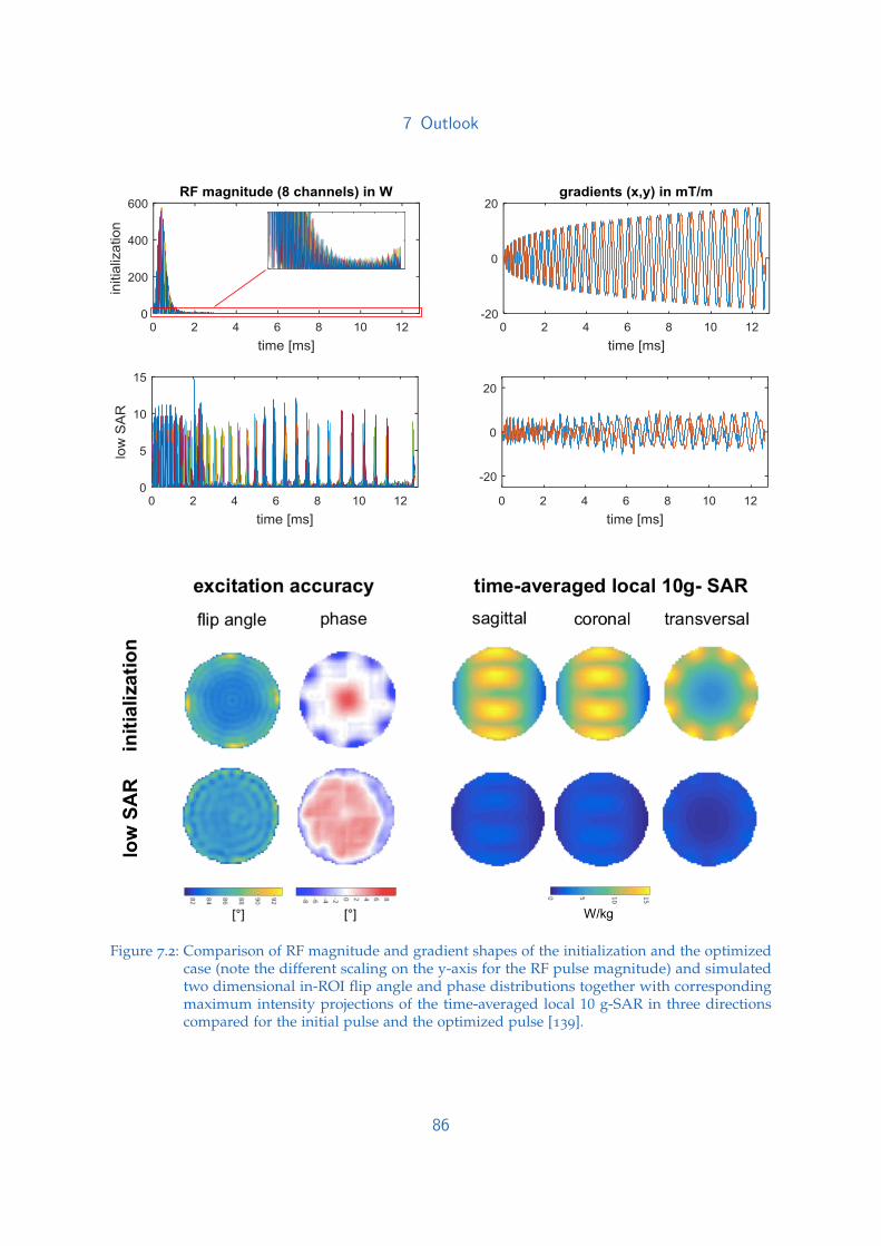
7 Outlook
Figure 7.2: Comparison of RF magnitude and gradient shapes of the initialization and the optimizedcase (note the different scaling on the y-axis for the RF pulse magnitude) and simulatedtwo dimensional in-ROI flip angle and phase distributions together with correspondingmaximum intensity projections of the time-averaged local 10 g-SAR in three directionscompared for the initial pulse and the optimized pulse [139].
86

8 List of Publications
Peer reviewed full journal publications
1. D. Bagga, C.S. Aigner, J.L. Reichert, C. Cecchetto, F.P.S. Fischmeister, P. Holzer,C. Moissl-Eichinger and V. Schopf. ”Influence of 4-week multi strain probioticadministration on resting-state functional connectivity in healthy volunteers”.European Journal of Nutrition, Early view May 2018, doi: https://doi.org/10.1007/s00394-018-1732-z
2. D. Bagga, J.L. Reichert, K. Koschutnig, C.S. Aigner, P. Holzer, K. Koskinen, C.Moissl-Eichinger and V. Schopf. ”Probiotics drive gut microbiome triggeringemotional brain signatures”. Gut Microbes, Early view May 2018, doi: https://doi.org/10.1080/19490976.2018.1460015
3. G. Pfurtscheller, A. Schwerdtfeger, A. Seither-Preisler, C. Brunner, C.S. Aigner,J. Calisto, J. Gens and A. Andrade. ”Synchronization of intrinsic 0.1-Hz blood-oxygen-level dependent (BOLD) oscillations in amygdala and prefrontal cortexin subjects with increased state anxiety”. European Journal of Neuroscience, Volume47:5, March 2018, Pages 417-426, doi: https://doi.org/10.1111/ejn.13845
4. A. Rund†, C.S. Aigner†, K. Kunisch, and R. Stollberger. ”Simultaneous multislicerefocusing via time optimal control”. Magnetic Resonance in Medicine, Early view:February 2018, doi: https://doi.org/10.1002/mrm.27124
5. A. Rund, C.S. Aigner, K. Kunisch, and R. Stollberger. ”Magnetic Resonance RFpulse design by optimal control with physical constraints”. IEEE Transactions onMedical Imaging, Volume 37:2, February 2018, Pages 461-472, doi: 10.1109/TMI.2017.2758391
6. S.M. Spann, K.S. Kazimierski, C.S. Aigner, M. Kraiger, K. Bredies, R. Stoll-berger. ”Spatio-temporal TGV denoising for ASL perfusion imaging”. NeuroIm-age, Volume 157, August 2017, Pages 81–96, doi: https://doi.org/10.1016/j.neuroimage.2017.05.054
7. G. Pfurtscheller, A. Schwerdtfeger, A. Seither-Preisler, C. Brunner, C.S. Aigner,J. Brito, M.P. Carmo, A. Andrade. ”Brain-heart communication: Evidence for
†Armin Rund and Christoph Stefan Aigner have contributed equally to the paper
87

8 List of Publications
”central pacemaker” oscillations with a dominant frequency at 0.1 Hz in thecingulum”. Clinical Neurophysiology, Volume 128:1, January 2017, Pages 183–193,doi: https://doi.org/10.1016/j.clinph.2016.10.097
8. G. Pfurtscheller, A. Schwerdtfeger , C. Brunner, C.S. Aigner, D. Fink, J. Brito,M.P. Carmo, A. Andrade. ”Distinction between Neural and Vascular BOLDOscillations and Intertwined Heart Rate Oscillations at 0.1 Hz in the RestingState and during Movement”. PLoS ONE 12(1): e0168097, January 2017, doi:https://doi.org/10.1371/journal.pone.0168097
9. C.S. Aigner, C. Clason, A. Rund and R. Stollberger. ”Efficient high-resolution RFpulse design applied to simultaneous multi-slice excitation”. Journal of MagneticResonance, Volume 263, February 2016, Pages 33–44, doi: https://doi.org/10.1016/j.jmr.2015.11.013
Peer reviewed conference proceedings
1. D. Bagga, C.S. Aigner, C. Cecchetto, F. Fischmeister, A. Specht, F. Schwaerzeland V. Schopf. ”The interplay between gender, GABA levels, and nicotineaddiction: A proton MRS investigation”. Annual OHBM Meeting, Singapore,Singapore, June 2018
2. C.S. Aigner, A. Rund, S. Abo Seada, S. Malik, J.V. Hajnal, K. Kunischand R. Stollberger. ”Time-optimal control based RF pulse design undergradient imperfections”. Proc. Intl. Soc. Mag. Reson. Med. 26, Paris, France,June 2018
3. A. Rund, C.S. Aigner, L. Nohava, R. Frass-Kriegl, E. Laistler, K. Kunisch and RStollberger. ”Optimal control based design of parallel transmission RF pulseswith minimum local SAR”. Proc. Intl. Soc. Mag. Reson. Med. 26, Paris, France,June 2018
4. S.M. Spann, C.S. Aigner, M. Schlogl, A. Lesch, K. Bredies, R. Stefan,D. Pinter, L. Pirpamer and R. Stollberger. ”Acceleration of arterial spinlabeling data using spatio-temporal total generalized variation (TGV)reconstruction”. Proc. Intl. Soc. Mag. Reson. Med. 26, Paris, France, June2018
5. S.M. Spann, M. Schlogl, C.S. Aigner, K. Koschutnig, M. Holler, K. Brediesand R. Stollberger. ”Denoising of functional Arterial Spin Labeling (fASL)perfusion data using infimal convolution of total generalized variationfunctionals (ICTGV)”. Proc. Intl. Soc. Mag. Reson. Med. 26, Paris, France,June 2018
88

8 List of Publications
6. A. Rund, C.S. Aigner, K. Kunisch and R. Stollberger. ”Magnetic ResonanceRadiofrequency Pulse Design by Optimal Control”. 9th Vienna Conference onMathematical Modelling, Vienna, Austria, January 2018
7. L. Nohava, A. Kuehne, C.S. Aigner, A. Rund, E. Moser, E. Laistler and R. FrassKriegl. ”Evaluation of RF pulses for 8-channel pTx systems at 7T with respectto hardware constraints and the trade-off between local 10g SAR and excitationaccuracy”. 34th ESMRMB Annual Scientific Meeting, Barcelona, Spain, October2017
8. D. Bagga, K. Koschutnig, B. Mohan, C.S. Aigner, J. Reichert, P. Holzer andV. Schopf. ”When gut speaks, brain listens: Exploring the influence of gutmicrobiota on emotional decision making”. Annual OHBM Meeting, Vancouver,Canada, June 2017
9. C.S. Aigner, A. Rund, B. Bilgic, B. Gagoski, K. Setsompop, K. Kunisch and R.Stollberger. ”Application of time-optimal Simultaneous Multi-Slice refocusingto TSE/RARE”. Proc. Intl. Soc. Mag. Reson. Med. 25, Hawaii, USA, April 2017
10. A. Rund, C.S. Aigner, K. Kunisch and R. Stollberger. ”Simultaneous multislicerefocusing by time-optimal control”. Proc. Intl. Soc. Mag. Reson. Med. 25, Hawaii,USA, April 2017
11. A. Rund, C.S. Aigner, K. Kunisch and R. Stollberger. ”RF pulse design byoptimal control with physical constraints”. Proc. Intl. Soc. Mag. Reson. Med. 25,Hawaii, USA, April 2017
12. A. Petrovic, C.S. Aigner and R. Stollberger. ”A time domain signal equation formulti-echo spin-echo sequences with arbitrary exciation and refocusing angleand phase”. Proc. Intl. Soc. Mag. Reson. Med. 25, Hawaii, USA, April 2017
13. M. Schloegl, S. Spann, C.S. Aigner, M. Holler, K. Bredies and R. Stollberger.”Improved Denoising of Dynamic Arterial Spin Labeling with Infimal Convolu-tion of Total Generalized Variation Functionals (ICTGV)”. Proc. Intl. Soc. Mag.Reson. Med. 25, Hawaii, USA, April 2017
14. S.M. Spann, K.S. Kazimierski, C.S. Aigner and R. Stollberger. ”A denoisingmethod for arterial spin labeling data based on total generalized variation (TGV)with a spatial varying regularization parameter”. Proc. Intl. Soc. Mag. Reson.Med. 25, Hawaii, USA, April 2017
15. D. Bagga, K. Koschutnig, B. Mohan, C.S. Aigner, J. Reichert, P. Holzer and V.Schopf. ”The Gut-Brain-Axis: from gut feelings to gut memory”. Proc. Intl. Soc.Mag. Reson. Med. 25, Hawaii, USA, April 2017
16. C.S. Aigner, C. Clason, A. Rund, A. Petrovic and R. Stollberger. ”Design ofcomplex RF pulse shapes for asymmetric excitation patterns via optimal control”.BMT 2016 ”Dreilandertagung“ Swiss, Austrian and German Societies of BiomedicalEngineering, Basel, Switzerland, October 2016
89

8 List of Publications
17. S.M. Spann, K.S. Kazimierski, C.S. Aigner, M. Kraiger and R. Stollberger; ”In-fluence of denoising techniques on the absolute CBF quantification of ASLperfusion data”. BMT 2016 ”Dreilandertagung“ Swiss, Austrian and German Soci-eties of Biomedical Engineering, Basel, Switzerland, October 2016
18. M. Bodenler, C.S. Aigner, A. Rund, C. Clason and R. Stollberger. Fast Optimiza-tion of RF Excitation. 33rd ESMRMB Annual Scientific Meeting, Vienna, Austria,October 2016
19. S.M. Spann, C.S. Aigner, K.S. Kazimierski, Markus Kraiger and R. Stollberger.”Total generalized variation (TGV) for spatio-temporal denoising of high reso-lution ASL perfusion data”. 33rd ESMRMB Annual Scientific Meeting, Vienna,Austria, October 2016
20. C.S. Aigner, C. Clason, A. Rund and R. Stollberger. ”Low SAR RF-pulse designby joint optimization of RF and gradient shape with physical constraints”. Proc.Intl. Soc. Mag. Reson. Med. 24, Singapore, Singapore, May 2016
21. C.S. Aigner, C. Clason, A. Rund and R. Stollberger. ”RF pulse design forsimultaneous multislice excitation with highly reduced B1 peak ampli-tude”. Proc. Intl. Soc. Mag. Reson. Med. 23, Toronto, Canada, June 2015;magna cum laude award
22. C.S. Aigner, C. Clason, A. Rund and R. Stollberger. ”SAR reduced excitation byjoint design of RF pulse and slice selective gradient shape”. Proc. Intl. Soc. Mag.Reson. Med. 23, Toronto, Canada, June 2015
23. A. Lesch, A. Petrovic, T.J. Sumpf, C.S. Aigner and R. Stollberger. ”Fast andAccurate Quantification of T1, T2 and Proton Density using IR bSSFP with SliceProfile Correction and Model Based Reconstruction”. Proc. Intl. Soc. Mag. Reson.Med. 23, Toronto, June 2015
24. C.S. Aigner, C. Clason, A. Rund and R. Stollberger. ”Validation of a flexibleoptimal control approach for RF-pulse-design including relaxation effects andSAR”. Annual Meeting of the Austrian Society for Biomedical Engineering, Hall inTirol, Austria, September 2014
25. C.S. Aigner, C. Clason, A. Rund and R. Stollberger. ”RF pulse design for lowSAR simultaneous multislice (SMS) excitation using optimal control”. Proc. Intl.Soc. Mag. Reson. Med. 22, Milano, Italy, May 2014
26. C.S. Aigner, C. Diwoky and R. Stollberger. ”Development of a pulseoximeter tomeasure the oxygen saturation and the heartrate of sedated mice”. BMT 2013
”Dreilandertagung“ Swiss, Austrian and German Societies of Biomedical Engineering,Graz, Austria, 2013
90

8 List of Publications
Oral Presentations
1. C.S. Aigner, A. Rund, S. Abo Seada, S. Malik, J.V. Hajnal, K. Kunisch andR. Stollberger. ”Time-optimal control based RF pulse design under gradientimperfections”. Intl. Soc. Mag. Reson. Med. 26 Power Pitch presentation,Paris, France, June 2018
2. C.S. Aigner. ”Spin Dance – On the Forefront of MRI Signal Generation”. 2ndHuman- and Biotechnology FoE Day, Graz, Austria, October 2017
3. C.S. Aigner, A. Rund, K. Kunisch and R. Stollberger. ”RF-Pulse Design withPhysical Constraints”. Czech-Austrian MR Workshop, Semmering, Austria, May2017
4. C.S. Aigner, A. Rund. ”Optimal Control Based Design of Tailored RF Pulses”.Invited Talk at the Medical University of Vienna, Vienna, Austria, October 2016
5. C.S. Aigner. ”Slice selective RF pulse design via optimal control”. Invited Talk atthe University Medical Center Freiburg, Freiburg, Germany, October 2016
6. C.S. Aigner, C. Clason, ”Design of complex RF pulse shapes for asymmetricexcitation patterns via optimal control”. BMT 2016 ”Dreilandertagung“ Swiss, Aus-trian and German Societies of Biomedical Engineering, Basel, Switzerland, October2016
7. C.S. Aigner, A. Rund. ”Towards tailored refocusing in minimum time: Re-sults and Application”. Imaging with Modulated/Incomplete Data, Graz, Austria,September 2016
8. C.S. Aigner, C. Clason, A. Rund and R. Stollberger. ”Low SAR RF-pulse designby joint optimization of RF and gradient shape with physical constraints”.Intl. Soc. Mag. Reson. Med. 24, Joint Study Group Session: High Field Systems andApplications and MR Safety, Singapore, Singapore, May 2016
9. C.S. Aigner, Christian Clason, Armin Rund and Rudolf Stollberger. ”RF PulseDesign With Optimal Control - Current and Future Applications”. SFB Sta-tusseminar 2016, Admont, Austria, April 2016
10. C.S. Aigner. ”Optimal Control – vom Raum zum Spin”. MRI research in Graz,Graz, Austria, March 2015
11. C.S. Aigner, Christian Clason, Armin Rund and Rudolf Stollberger. ”RF PulseOptimization via Optimal Control – Summary and Outlook”. SFB NetworkingSeminar 2014, Graz, Austria, September 2014
12. C.S. Aigner, C. Clason, A. Rund and R. Stollberger. ”RF pulse design forsimultaneous multislice excitation with highly reduced B1 peak ampli-tude”. Proc. Intl. Soc. Mag. Reson. Med. 23, Toronto, Canada, June 2015;magna cum laude award
91

8 List of Publications
13. C.S. Aigner, C. Clason, A. Rund and R. Stollberger. ”Validation of a flexibleoptimal control approach for RF-pulse-design including relaxation effects andSAR”. Annual Meeting of the Austrian Society for Biomedical Engineering, Hall inTirol, Austria, September 2014
14. C.S. Aigner, Christian Clason, Armin Rund and Rudolf Stollberger. ”Opti-mal control for advanced 1D RF-pulse-design: Results and Challenges”. SFBStatusseminar 2013, Admont, Austria, November 2013
15. C.S. Aigner, Christian Clason, Armin Rund and Rudolf Stollberger. ”An optimalcontrol approach for advanced 1D RF-pulse-design including relaxation effects”.BMT 2013 ”Dreilandertagung“ Swiss, Austrian and German Societies of BiomedicalEngineering, Graz, Austria, September 2013
Prices, Awards and Stipends
1. Magna cum laude award ISMRM 26 (2018), Paris, France2. 1st place in the ISMRM RF pulse design challenge 2015: Simultaneous Multislice
Acquisition. Member of the winning team ”rfcontrol” together with A.Rund,C.Clason, K.Kunisch and R. Stollberger; (2015-2016), SingaporeMRM Highlights: Q&A with 2015 ISMRM Challenge Winners, (http://www.ismrm.org/rf-pulse-design-challenge/)MRM full paper: W. Grissom and K. Setsompop et al., MRM 2016. (https://doi.org/10.1002/mrm.26512)
3. Magna cum laude award ISMRM 23 (2015), Toronto, Canada4. ISMRM Educational Stipend 2014, 2015 and 2016
92

9 Appendix
9.1 Efficient high-resolution RF pulse design applied tosimultaneous multi-slice excitation
Christoph Stefan Aigner1,2, Christian Clason3, Armin Rund4 and Rudolf Stoll-berger1,2
This is a preprint of the publication ”Efficient high-resolution RF pulse design appliedto simultaneous multi-slice excitation”. Journal of Magnetic Resonance, Volume 263,February 2016, Pages 33–44, doi: https://doi.org/10.1016/j.jmr.2015.11.013
Abstract
RF pulse design via optimal control is typically based on gradient and quasi-Newtonapproaches and therefore suffers from slow convergence. We present a flexible andhighly efficient method that uses exact second-order information within a globallyconvergent trust-region CG-Newton method to yield an improved convergence rate.The approach is applied to the design of RF pulses for single- and simultaneousmulti-slice (SMS) excitation and validated using phantom and in-vivo experimentson a 3 T scanner using a modified gradient echo sequence.
1Institute of Medical Engineering, Graz University of Technology, Stremayrgasse 16, 8010 Graz, Austria2BioTechMedGraz, 8010 Graz, Austria3Faculty of Mathematics, University of Duisburg-Essen, 45117 Essen, Germany4Institute for Mathematics and Scientific Computing, University of Graz, Heinrichstrasse 36, 8010
Graz, Austria
93

9 Appendix
9.1.1 Introduction
For many applications in MRI there is still demand for the optimization of selectiveRF excitation, e.g., for simultaneous multi-slice excitation [163], [166], UTE imaging[198], or velocity selective excitation [128]. To achieve a well-defined slice profile athigh field strength while meeting B1 peak amplitude limitations is a challenge for RFpulse design and becomes especially critical for quantitative methods.
Correspondingly, many approaches for general pulse design have been proposed inthe literature. RF pulses with low flip angles can be designed using the small tip anglesimplification [43], which makes use of an approximation of the Bloch equation tocompute a pulse via the Fourier transform of the desired slice profile. However, thissimplification breaks down for large flip angles. The resulting excitation error for largeflip angle pulses can be reduced by applying the Shinnar–Le Roux (SLR) technique[66] or optimization methods, e.g., simulated annealing, evolutionary approaches oroptimal control [47], [120], [147], [149], [152], [153], [199]. The SLR method is basedon the hard pulse approximation and a transformation of the excitation problem,allowing to solve the excitation problem recursively by applying fast filter designalgorithms such as the Parks–McClellan algorithm [66]. Originally, this approachonly covered special pulses such as 90 and 180 excitation or refocusing, but Lee[200] generalized this approach to arbitrary flip angles with an exact parameterrelation. Despite its limitations due to neglected relaxation terms and sensitivity to B1inhomogeneities, it found widespread use (see, e.g., [200]–[203]) and is considered tobe the gold standard for large tip angle pulse design. An alternative approach is basedon optimizing a suitable functional; see, e.g., [47], [66], [145], [151], [154]. In particular,optimal control (OC) approaches involve the solution of the Bloch equation describingthe evolution of the magnetization vector in an exterior magnetic field [47], [49], [120],[152], [153], [155], [156], [182]. They often lead to better excitation profiles due to amore accurate design model and are increasingly used in MRI, for instance, to performmultidimensional and multichannel RF design [47], [49], robust 2D spatial selectivepulses [153] and saturation contrast [152]. In addition, arbitrary flip angles and targetslice profiles, as well as inclusion of additional physical effects such as, e.g., relaxationcan be handled. However, so far OC approaches are limited by the computationaleffort and require a proper modeling of the objective. In particular, standard gradient-based approaches suffer from slow convergence, imposing significant limitationson the accuracy of the obtained slice profiles. On the other hand, Newton methodsshow a locally quadratic convergence, but require second-order information whichin general is expensive to compute [157]. Approximating the Hessian using finitedifferences causes loss of quadratic convergence due to the lack of exact second-order information and typically requires significantly more iterations. Superlinearconvergence can be obtained using quasi-Newton methods based on exact gradients
94

9 Appendix
[204], although their performance can be sensitive to implementation details. Thepurpose of this work is to demonstrate that for the OC approach to pulse design,it is in fact possible to use exact second-order information while avoiding the needof computing the full Hessian, yielding a highly efficient numerical method for theoptimal control of the full time-dependent Bloch equation. In contrast to [157] (whichuses black-box optimization method and symbolically calculated Hessians based onan effective-matrix approximation of the Bloch equation), we propose a matrix-freeNewton–Krylov method [186] using first- and second-order derivatives based on theadjoint calculus [205] together with a trust-region globalization [185]; for details werefer to Section 9.1.2. Recently, similar matrix-free Newton–Krylov approaches withline search globalization were presented for optimal control of quantum systems inthe context of NMR pulse sequence design [206], [207]. In comparison, the proposedtrust-region framework significantly reduces the computational effort, particularlyfor the initial steps far away from the optimum. The effectiveness of the proposedmethod is demonstrated for the design of pulses for single and simultaneous multi-slice excitation (SMS).
SMS excitation is increasingly used to accelerate imaging experiments [163]–[166].Conventional design approaches, based on a superposition of phase-shifted sub-pulses [162] or sinusoidal modulation [163], typically result in a linear scaling ofthe B1 peak amplitude, a quadratic peak power and a linear increase in the overallRF power [131], [175]. The required maximal B1 peak amplitude of conventionalmulti-slice pulses therefore easily exceeds the transmit voltage of the RF amplifier. Inthis case, clipping will occur, while rescaling will decrease and limit the maximal flipangle of such a pulse. On the other hand, restrictions of the specific absorption ratelimit the total (integrated) B1 power and therefore the maximal number of slices aswell as the pulse duration and flip angle. The increase of B1 power can be addressedby the Power Independent of Number of Slices (PINS) technique [131], which wasextended to the kT-PINS method [208] to account for B1 inhomogeneities. Thisapproach leads to a nearly slice-independent power requirement, but the periodicityof the resulting excitation restricts the slice orientation and positioning. Furthermore,the slice profile accuracy is reduced [165], and a limited ratio between slice thicknessand slice distance may further restrict possible applications. The combination of PINSwith regular multi-band pulses was shown to reduce the overall RF power by up to50 % (MultiPINS [179]) and was applied to refocusing pulses in a multi-band RAREsequence with 13 slices [195].
A different way to reduce the maximum B1 amplitude is to increase the pulse length;however, this stretching increases the minimal echo and repetition times and decreasesthe RF bandwidth, thus reducing the slice profile accuracy [175]. Applying variablerate selective excitation [160], [209] avoids this problem but leads to an increasedsensitivity to slice profile degradations at off-resonance frequencies. In addition, they
95

9 Appendix
require specific sequence alterations, e.g., variable slice gradients or gradient blips.Instead of using the same phase for all sub-slices, the peak power can be reducedby changing the uniform phase schedule to a different phase for each individualslice [174]. Alternative approaches[173], [210] using phase-matched excitation andrefocusing pairs show that a nonlinear phase pattern can be corrected by a subsequentrefocusing pulse. Another way to reduce the power deposition and SAR of SMS pulsesis to combine them with parallel transmission [211]. This allows to capitalize transmitsensitivities in the pulse design and leads to a more uniform excitation with anincreased power efficiency [212], [213]. Recently, Guerin et al. [214] demonstrated thatit is possible to explicitly control both global and local SAR as well as the peak powerusing a spokes-SMS-pTx pulse design.
The focus of this work, however, is on single channel imaging, where we apply ourOC-based pulse design for efficient SMS pulse optimization using a direct descriptionof the desired magnetization pattern. Its flexible formulation allows a trade-offbetween the slice profile accuracy and the required pulse power and is well suitedfor the reduction of power and amplitude requirements of such pulses, even for alarge number of slices or large flip angles or in presence of relaxation. The efficientimplementation of the proposed method allows to optimize for SMS pulses witha high spatial resolution to achieve accurate excitation profiles. The RF pulses aredesigned to achieve a uniform effective echo time and phase for each slice anduse a constant slice-selective gradient, allowing to insert the RF pulse into existingsequences and opening up a wide range of applications.
9.1.2 Theory
This section is concerned with the description of the optimal control approach to RFpulse design as well as of the proposed numerical solution approach.
Optimal control framework
Our OC approach is based on the full time-dependent Bloch equation, whichdescribes the temporal evolution of the ensemble magnetization vector M(t) =(Mx(t), My(t), Mz(t))T due to a transient external magnetic field B(t) as the solutionof the ordinary differential equation (ODE)
M(t) = γB(t)×M(t) + R(M(t)), t > 0,
M(0) = M0,(9.1)
96

9 Appendix
where γ is the gyromagnetic ratio, M0 is the initial magnetization and
R(M(t)) = (−Mx(t)/T2,−My(t)/T2,−(Mz(t)−M0)/T1)T (9.2)
denotes the relaxation term with relaxation times T1, T2 and the equilibrium mag-netization M0. To encode spatial information in MR imaging, the external magneticfield B (and thus the magnetization vector) depends on the slice direction z, hencethe Bloch equation can be considered as a parametrized family of three-dimensionalODEs. In the on-resonance case and ignoring spatial field inhomogeneities, the Blochequation can be expressed in the rotating frame as
M(t; z) = A(u(t); z)M(t; z) + b(z), t > 0,
M(0; z) = M0(z),(9.3)
where the control u(t) = (ux(t), uy(t)) describes the RF pulse,
A(u; z) =
− 1T2
γGz(t)z γuy(t)B1
−γGz(t)z − 1T2
γux(t)B1
−γuy(t)B1 −γux(t)B1 − 1T1
, b(z) =
00
M0T1
, (9.4)
and Gz is the slice-selective gradient; see, e. g., [26, Chapter 6.1].
The OC approach consists in computing for given initial magnetization M0(z) theRF pulse u(t), t ∈ [0, Tu], that minimizes the squared error at read-out time T > Tubetween the corresponding solution M(T; z) of (9.3) and a prescribed slice profileMd(z) for all z ∈ [−a, a] together with a quadratic cost term modeling the SAR of thepulse, i.e., solving
min(u,M) satisfying (9.3)
J(M, u) =12
∫ a
−a|M(T; z)−Md(z)|22 dz +
α
2
∫ Tu
0|u(t)|22 dt. (9.5)
The parameter α > 0 controls the trade-off between the competing goals of sliceprofile attainment and SAR reduction.
Adjoint approach
The standard gradient method for solving (9.5) consists of computing for given uk
the gradient g(uk) of j(u) := J(M(u), u) and setting uk+1 = uk − skg(uk) for some
97

9 Appendix
suitable step length sk. The gradient can be calculated efficiently using the adjointmethod, which in this case yields
g(uk)(t) = αu(t) + γB1
(∫ a−a Mz(t; z)Py(t; z)−My(t; z)Pz(t; z) dz∫ a−a Mz(t; z)Px(t; z)−Mx(t; z)Pz(t; z) dz
)
=: αu(t) +
(∫ a−a M(t; z)A1P(t; z) dz∫ a−a M(t; z)A2P(t; z) dz
), 0 ≤ t ≤ Tu,
(9.6)
where M is the solution to (9.3) for u = uk and 0 < t ≤ T, P is the solution to theadjoint (backward in time) equation
−P(t; z) = A(u(t); z)TP(t; z), 0 ≤ t < T,P(T; z) = M(T; z)−Md(z),
(9.7)
and for the sake of brevity, we have set
A1 := γB1
0 0 00 0 −10 1 0
, A2 := γB1
0 0 −10 0 01 0 0
. (9.8)
However, this method requires a line search to converge and usually suffers fromslow convergence close to a minimizer. This is not the case for Newton’s method(which is a second-order method and converges locally quadratically), where oneadditionally computes the Hessian H(uk) of j at uk, solves for δu in
H(uk)δu = −g(uk), (9.9)
and sets uk+1 = uk + δu. While the full Hessian H(uk) is very expensive to computein practice, solving (9.9) using a Krylov method such as conjugate gradients (CG) onlyrequires computing the Hessian action H(uk)h for a given direction h per iteration;see, e.g., [186]. The crucial observation in our approach is that the adjoint methodallows computing this action exactly (e.g., without employing finite difference ap-proximations) and without knowledge of the full Hessian. Since Krylov methodsusually converge within very few iterations, this so-called “matrix-free” approachamounts to significant computational savings. To derive a procedure for computingthe Hessian action H(uk)h for a given direction h directly, we start by differentiating(9.6) with respect to u in direction h and applying the product rule. This yields
98

9 Appendix
[H(uk)h](t) = αh(t) +(∫ a−a δM(t; z)A1P(t; z) + M(t; z)A1δP(t; z) dz∫ a−a δM(t; z)A2P(t; z) + M(t; z)A2δP(t; z) dz
), 0 ≤ t ≤ Tu, (9.10)
where δM – corresponding to the directional derivative of M with respect to u – isgiven by the solution of the linearized state equation
˙δM(t; z) = A(uk; z)δM(t; z) + A′(h)M, 0 < t ≤ T,
δM(0; z) = (0, 0, 0)T,(9.11)
with
A′(h) = γB1
0 0 hy(t)0 0 hx(t)
−hy(t) −hx(t) 0
, (9.12)
and δP – corresponding to the directional derivative of P with respect to u – is thesolution of the linearized adjoint equation
− ˙δP(t; z) = A(uk; z)TδP(t; z) + A′(h)TP, 0 ≤ t < T,δP(T; z) = δM(T; z).
(9.13)
This characterization can be derived using formal Lagrangian calculus and rigorouslyjustified using the implicit function theorem; see, e.g., [215, Chapter 1.6]. Since (9.10)can be computed by solving the two ODEs (9.11) and (9.13), the cost of computing asingle Hessian action is comparable to that of a gradient evaluation; cf. (9.6). This hasalready been observed in the context of seismic imaging [216], meteorology [217], andoptimal control of partial differential equations [205], but has received little attentionso far in the context of optimal control of ODEs.
One difficulty is that the Bloch equation (9.3) is bilinear since it involves the product ofthe unknowns u and M. Hence, the optimal control problem (9.5) is not convex and theHessian H(u) is not necessarily positive definite (or even invertible), thus precluding adirect application of the CG-Newton method. We therefore embed Newton’s methodinto the trust-region framework of Steihaug [185], where a breakdown of the CGmethod is handled by a trust-region step and the trust region radius is continuallyadapted. This allows global convergence (i.e., for any starting point) to a localminimizer as well as transition to fast quadratic convergence; see [185]. As an addedadvantage, computational time is saved since the CG method is usually not fullyresolved far away from the optimum. The full algorithm is given in Appendix 9.1.7.
99

9 Appendix
Discretization
For the numerical computation of optimal controls, both the Bloch equation (9.3)and the optimal control problem in (9.5) need to be discretized. Here, the timeinterval [0, T] is replaced by a time grid 0 = t0 < · · · < tN = T with time steps∆tm := tm − tm−1, chosen such that tNu = Tu < T for some Nu < N. The domain[−a, a] is replaced by a spatial grid −a = z1 < · · · < zZ = a with grid sizes∆zm := zm − zm−1. We note that for each zi, the corresponding ODEs can be solvedindependently and in parallel. The Bloch equation is discretized using a Crank–Nicolson method, where the state M is discretized as continuous piecewise linearfunctions with values Mm := M(tm), and the controls u are treated as piecewiseconstant functions, i.e., u = ∑Nu
m=1 umχ(tm−1,tm](t), where χ(a,b] is the characteristicfunction of the half-open interval (a, b].
For the efficient computation of optimal controls, it is crucial that both the gradientand the Hessian action are computed in a manner consistent with the chosen dis-cretization. This implies that the adjoint state P has to be discretized as piecewiseconstant using an appropriate time-stepping scheme [218], and that the linearizedstate δM and the linearized adjoint state δP have to be discretized in the same way asthe state and adjoint state, respectively. Furthermore, the conjugate gradient methodhas to be implemented using the scaled inner product 〈u, v〉 := ∑Nu
m=1 ∆tmumvm andthe corresponding induced norm ‖u‖2 := 〈u, u〉. For completeness, the resultingschemes and discrete derivatives are given in Appendix 9.1.8.
9.1.3 Methods
This section describes the computational implementation of the proposed pulsedesign and the experimental protocol for its validation.
Pulse design
The OC approach described in Section 9.1.2 is implemented in MATLAB (The Math-Works, Inc., Natick, USA) using the Parallel Toolbox for parallel solution of the(linearized) Bloch and adjoint equation for different values of zi. In the spirit ofreproducible research, the code used to generate the results in this paper can bedownloaded from https://github.com/chaigner/rfcontrol/releases/v1.2.
100

9 Appendix
−0.01 −0.005 0 0.005 0.01
0
1
z [m]
norm
aliz
ed m
ag
ne
tiza
tion
Md,x
Md,y
Md,z
−0.01 −0.005 0 0.005 0.01
0
1
z [m]
norm
aliz
ed m
ag
ne
tiza
tion
(a) Md for single slice (zoom)
−0.1 −0.05 0 0.05 0.1
−1
0
1
z [m]n
orm
aliz
ed m
ag
ne
tiza
tion
Md,x
Md,y
Md,z
−0.1 −0.05 0 0.05 0.1
−1
0
1
z [m]n
orm
aliz
ed m
ag
ne
tiza
tion
(b) Md for SMS 6 (zoom)
−0.1 −0.05 0 0.05 0.1
−1
0
1
z [m]
norm
aliz
ed m
ag
ne
tiza
tion
Md,x
Md,y
Md,z
−0.1 −0.05 0 0.05 0.1
−1
0
1
z [m]
norm
aliz
ed m
ag
ne
tiza
tion
(c) Md for phase shifted SMS6 (zoom)
Figure 9.1: Desired magnetization for single- (a) and multi-slice (b,c) pulse design
The initial magnetization vector is set to equilibrium, i.e., M0(z) = M0(0, 0, 1)T. Theslice-selective gradient Gz(t) is extracted out of a standard Cartesian GRE sequencesimulation and consists of a trapezoidal shape of length 2.56 ms that is followed by are-phasing part of length 0.92 ms to correct the phase dispersion using the maximalslew rate; i.e., Tu = 2.56 ms and T = 3.48 ms with a temporal resolution of ∆t = 5 µsfor the single-slice excitation (see dashed line in Figure 9.2a) and Tu = 10.24 ms andT = 13.92 ms with a temporal resolution of ∆t = 20 µs for the SMS excitation (seedashed line in Figure 9.4a). This corresponds in both cases to N = 697 uniform timesteps for the time interval [0, T] and Nu = 512 time steps for the control interval[0, Tu]. For the spatial computational domain, a = 0.5 m is chosen to consider typicalscanner dimensions; the domain [−a, a] is discretized using Z = 5001 equidistantpoints to achieve a homogeneous spatial resolution of ∆z = 0.2 mm.
For the desired magnetization vector, we consider three examples:
Single-slice excitation To validate the design procedure, we compute an optimizedpulse for a single slice of a given thickness ∆w and a flip angle of 90, i.e., we set
Md(z) =
(0, sin(90), cos(90))T if |z| < ∆w/2,(0, 0, 1)T else,
(9.14)
as visualized in Figure 9.1a. To reduce Gibbs ringing, this vector is filtered before theoptimization with a Gaussian kernel with a full width at half maximum of 1.6 mm.For comparison, an SLR pulse [66], [200] with an identical temporal resolution andpulse duration is designed to the same specification (slice width, flip angle, full widthat half maximum) using the Parks–McClellan (PM) algorithm [66] with a 1 % in-
101

9 Appendix
and out-of slice ripple as usual [66] and a bandwidth of 2.35 kHz. To achieve a fullyrefocused magnetization, the refocusing area of the slice selective gradient for theSLR pulse is increased by 4.1 percent compared to the OC pulse (Figure 9.2a).
SMS excitation: phantom RF pulses for the simultaneous excitation of two, four,and six equidistant rectangular slices with a flip angle of 90 are computed, i.e., weset
Md(z) =
(0, sin(90), cos(90))T if z in slice,(0, 0, 1)T if z out of slice,
(9.15)
and apply Gauss filtering; see Figure 9.1b for the case of six slices.
Since PINS pulses are not suitable for axial or axial-oblique slice preference asthey generate a periodic slice pattern extending outside the field of interest [166],the optimized pulses are compared with conventional SMS pulses obtained usingsuperposed phase-shifted sinc-based excitation pulses, again for the same slice width,flip angle and full width at half maximum.
SMS excitation: in-vivo Since multi-slice in-vivo imaging using slice-GRAPPA startsto suffer from g-factor problems for more than three slices, we modify the above-described SMS pulses using a CAIPIRINHA-based excitation pattern [171], whichalternates two different pulses to achieve phase-shifted magnetization vectors in orderto increase the spatial distance of aliased voxels. Here, the first vector and pulseare identical to those designed for the phantom. For odd slice numbers, the secondvector is modified by adding a phase term of π to every second slice of the desiredmagnetization, i.e.,
Md(z) =
(0,± sin(90), cos(90))T if z in odd/even slice,(0, 0, 1)T if z out of slice
(9.16)
(before filtering). For even slice numbers, the transverse pattern has to be furthershifted by π
2 , i.e.,
Md(z) =
(± sin(90), 0, cos(90))T if z in even/odd slice,(0, 0, 1)T if z out of slice,
(9.17)
see Figure 9.1c for the case of six slices. The additional phase shift is balanced beforereconstruction by subtracting a phase of π
2 from every second phase-encoding lineof the measured k-space data. Since typical relaxation times in the human brain are
102

9 Appendix
at least an order of magnitude bigger than the pulse duration, relaxation effects areneglected in the optimization.
The starting point for the optimization is chosen in all cases as u0 = [0, . . . , 0]. Thecontrol cost parameter is fixed at α = 10−4 for both the single-slice and the multi-sliceoptimization. The parameters in Algorithm 1 are set to tolN = 10−9, maxitN = 5,tolC = 10−6, maxitC = 50, ρ0 = 1, ρmax = 2, q = 2, σ1 = 0.03, σ2 = 0.25, σ3 = 0.7.
All calculations are performed on a workstation with a four-core 64 bit processor with3.1 GHz (Intel i5-3350P) and 16 GB of RAM.
Experimental validation
Fully sampled experimental data for a phantom and a healthy volunteer were acquiredon a 3 T MR scanner (Magnetom Skyra, Siemens Healthcare, Erlangen, Germany)using the built-in body coil to transmit the RF pulse. The MR signals were receivedusing a body coil for the phantom experiments and a 32-channel head coil for thein-vivo experiments. A standard Cartesian GRE sequence was modified to import andapply external RF pulses. By changing the read-out gradient from the frequency-axisto the slice direction, the excited slice can be measured and visualized. The single-sliceexcitation was measured using a water filled sphere with a diameter of 170 mm. Toacquire a high resolution in z-direction, we used a matrix size of 512× 384 with a FOVof 250 mm× 187 mm and a bandwidth of 390 Hz. The echo time was TE = 5 ms andthe repetition time TR = 2000 ms to get fully relaxed magnetization before the nextexcitation. The SMS phantom experiments were performed using a homogeneouscylinder phantom with diameter of 140 mm, length of 400 mm, and relaxation timesT1 = 102 ms, T2 = 81 ms, and T∗2 = 70 ms. The sequence parameters were TE =10 ms, TR = 1000 ms, bandwidth 390 Hz, matrix size 512× 288, and a field of view of250 mm× 141 mm.
To verify the in-vivo applicability, human brain images of a healthy volunteer wereacquired using the above described GRE sequence modified to include the optimizedCAIPIRINHA-based pulses. The sequence parameters were set to TE = 10 ms, TR =4000 ms, bandwidth 390 Hz, matrix size 192× 120 and FOV 300 mm× 187 mm. Afteracquisition, the k-space data of the individual slices were separated using an offlineslice-GRAPPA (32 coils, kernel size of 4× 4) reconstruction [172], [219]. The referencescans used in the slice-GRAPPA reconstruction were performed with the samesequence using an optimized single-slice pulse (not shown here). To decrease thescanning time, we acquired 25 k-space lines (1/5 of the full dataset) around the
103

9 Appendix
k-space center for each reference scan. After this separation, a conventional Cartesianreconstruction was performed individually for each slice.
9.1.4 Results
Single-slice excitation Figure 9.2 shows the results of the design of an RF pulse forthe excitation of a single slice of width ∆w = 5 mm; see Figure 9.1a. The computedpulse (after 4 Newton iterations and a total number of 28 CG steps taking 989 s onthe above-mentioned workstation is shown in Figure 9.2a. (To indicate the sequencetiming, the slice-selective gradient Gz – although not part of the optimization – isshown dashed.) It can be seen that ux(t) is similar, but not identical, to a standardsinc shape, and that uy(t) is close to zero, which is expected due to the symmetryof the prescribed slice profile. Figure 9.2b contains a detail of the correspondingtransverse magnetization Mxy(T) = (Mx(T)2 + My(T)2)1/2 obtained from the nu-merical solution of the Bloch equation, which is confirmed by experimental phantommeasurements in Figure 9.2c,d. Both simulation and measurement show an excitationwith a steep transition between the in- and out-of-slice regions and a homogeneousflip angle distribution across the target slice.
Figure 9.3 compares the optimized (OC) pulse with a standard SLR pulse by showingdetails of the corresponding simulated magnetizations (Figure 9.3a for OC and Figure9.3b for SLR; in both cases the targeted ideal magnetization is shown dashed). Itcan be seen that the in-slice magnetization of the optimized pulse has oscillations ofhigher frequency but of much smaller amplitude than that of the SLR pulse. Thisbecomes especially visible when comparing the resulting in-slice phases (Figure9.3c).
This is achieved by allowing higher ripples close to the slice while decreasing theamplitude monotonically away from the slice. (Note that only a small central segmentof this region is shown in the figures.) This leads to the total root mean squared error(RMSE) and the mean absolute error (MAE) with the ideal rectangular magnetizationpattern (Figure 9.3d) matching the full width at half maximum of both pulses beingsmaller for the OC pulse (1.46× 10⁻² and 1.10× 10⁻⁴, respectively) compared tothe SLR pulse (1.62× 10⁻² and 2.27× 10⁻⁴, with an equal power demand for bothpulses.
SMS excitation: phantom Figure 9.4 shows the results of the design of RF pulsesfor simultaneous excitation of two, four and six equidistant slices with a separation
104
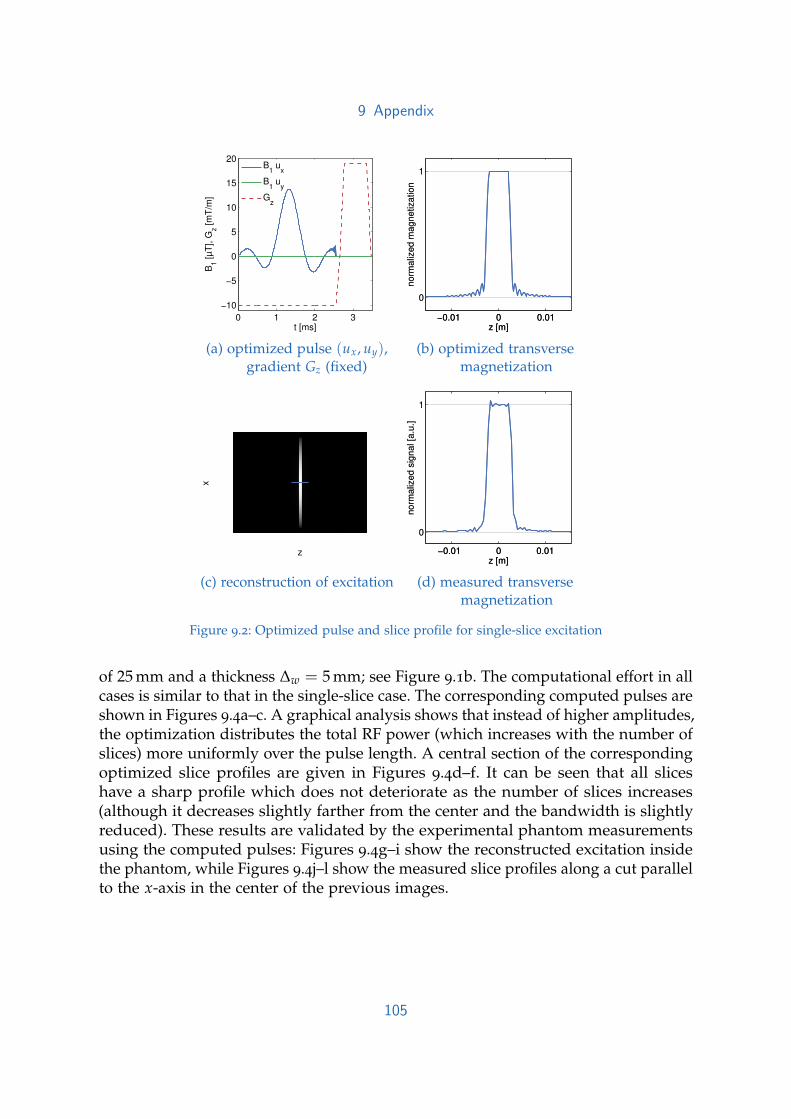
9 Appendix
0 1 2 3
−10
−5
0
5
10
15
20
t [ms]
B1 [µT
], G
z [m
T/m
]
B
1 u
x
B1 u
y
Gz
(a) optimized pulse (ux, uy),gradient Gz (fixed)
−0.01 0 0.01
0
1
z [m]
norm
aliz
ed m
agnetization
−0.01 0 0.01
0
1
z [m]
norm
aliz
ed m
agnetization
(b) optimized transversemagnetization
z
x
(c) reconstruction of excitation
−0.01 0 0.01
0
1
z [m]
norm
aliz
ed s
ignal [a
.u.]
−0.01 0 0.01
0
1
z [m]
norm
aliz
ed s
ignal [a
.u.]
(d) measured transversemagnetization
Figure 9.2: Optimized pulse and slice profile for single-slice excitation
of 25 mm and a thickness ∆w = 5 mm; see Figure 9.1b. The computational effort in allcases is similar to that in the single-slice case. The corresponding computed pulses areshown in Figures 9.4a–c. A graphical analysis shows that instead of higher amplitudes,the optimization distributes the total RF power (which increases with the number ofslices) more uniformly over the pulse length. A central section of the correspondingoptimized slice profiles are given in Figures 9.4d–f. It can be seen that all sliceshave a sharp profile which does not deteriorate as the number of slices increases(although it decreases slightly farther from the center and the bandwidth is slightlyreduced). These results are validated by the experimental phantom measurementsusing the computed pulses: Figures 9.4g–i show the reconstructed excitation insidethe phantom, while Figures 9.4j–l show the measured slice profiles along a cut parallelto the x-axis in the center of the previous images.
105

9 Appendix
−0.01 0 0.01
0
1
z [m]
norm
aliz
ed m
agnetization
Mx(T)
My(T)
Mz(T)
|Mi,xy
|
−0.01 0 0.01
0
1
z [m]
norm
aliz
ed m
agnetization
(a) simulated magnetization(OC)
−0.01 0 0.01
0
1
z [m]
norm
aliz
ed m
agnetization
Mx(T)
My(T)
Mz(T)
|Mi,xy
|
−0.01 0 0.01
0
1
z [m]
norm
aliz
ed m
agnetization
(b) simulated magnetization(SLR)
−2 −1 0 1 2
x 10−3
−0.5
0
0.5
z [m]
phase [ra
d]
SLR
OC
−2 −1 0 1 2
x 10−3
−0.5
0
0.5
z [m]
phase [ra
d]
(c) in-slice phase
−0.01 0 0.01
0
1
z [m]
norm
aliz
ed m
agnetization
Mi,x
Mi,y
Mi,z
−0.01 0 0.01
0
1
z [m]
norm
aliz
ed m
agnetization
(d) ideal magnetization
Figure 9.3: Comparison of SLR and OC pulse
A quantitative comparison of SLR and OC-based SMS pulses from one to six simulta-neous slices is given in Table 9.1, which shows both the power requirement of thecomputed pulses, both in total B1 energy
‖B1,x‖22 =
∫ T
0|B1ux(t)|2 dt (9.18)
and in peak B1 amplitude
‖B1,x‖∞ = maxt∈[0,T]
|B1ux(t)|, (9.19)
as well as the mean absolute error (MAE) with respect to the ideal (unfiltered) sliceprofiles for the in-slice and the out-of-slice regions. While both methods lead to alinear increase of the total energy with the number of slices, the peak amplitude in-creases more slowly for the OC pulses than for the conventional pulses. Furthermore,we remark that the peak B1 amplitude for four, five and six slices remain similar.
106

9 Appendix
0 5 10−15
0
15
time [ms]
B1 [µT
], G
z [m
T/m
]
B
1 u
x
B1 u
y
Gz
(a) optimized pulse (2slices)
0 5 10−15
0
15
time [ms]
B1 [µT
], G
z [m
T/m
]
B
1 u
x
B1 u
y
Gz
(b) optimized pulse (4slices)
0 5 10−15
0
15
time [ms]
B1 [µT
], G
z [m
T/m
]
B
1 u
x
B1 u
y
Gz
(c) optimized pulse (6slices)
−0.05 0 0.050
0.5
1
z [m]
norm
aliz
ed m
agnetization
−0.05 0 0.050
0.5
1
z [m]
norm
aliz
ed m
agnetization
(d) optimized slice pro-file (2)
−0.05 0 0.050
0.5
1
z [m]
norm
aliz
ed m
agnetization
−0.05 0 0.050
0.5
1
z [m]
norm
aliz
ed m
agnetization
(e) optimized slice pro-file (4)
−0.05 0 0.050
0.5
1
z [m]
norm
aliz
ed m
agnetization
−0.05 0 0.050
0.5
1
z [m]
norm
aliz
ed m
agnetization
(f) optimized slice pro-file (6)
z
x
(g) reconstructed excita-tion (2)
z
x
(h) reconstructed excita-tion (4)
z
x
(i) reconstructed excita-tion (6)
−0.05 0 0.050
500
1000
1500
2000
position in m
sig
nal [a
.u.]
(j) measured slice pro-file (2)
−0.05 0 0.050
500
1000
1500
2000
position in m
sig
nal [a
.u.]
(k) measured slice pro-file (4)
−0.05 0 0.050
500
1000
1500
2000
position in m
sig
nal [a
.u.]
(l) measured slice pro-file (6)
Figure 9.4: Optimized pulses and slice profiles for SMS excitation (phantom)
107

9 Appendix
Regarding the corresponding slice profiles, the OC pulses lead to a significantly lowerMAE in both the in-slice and out-of-slice regions compared to the SLR pulses. Visualinspection of Figure 9.4d–f shows that this is due to the fact that the out-of-sliceripples are concentrated around the in-slice regions while quickly decaying awayfrom them.
Table 9.1: Comparison of B1 power and the mean absolute error (MAE) of the transverse magnetizationafter excitation for conventional and OC based SMS pulses
‖B1,x‖22 ‖B1,x‖∞ MAE in-slice MAE out-of-slice
[a.u.] [µT] [a.u.] [a.u.]
slices conv OC conv OC conv OC conv OC
1 19.5 19.5 3.5 3.49 0.062 0.052 0.0039 0.00142 38.9 38.1 7.0 6.78 0.060 0.052 0.0040 0.00183 58.4 57.2 10.5 10.02 0.054 0.053 0.0039 0.00304 77.9 76.3 14.0 12.13 0.065 0.045 0.0086 0.00315 97.3 95.5 17.5 11.38 0.059 0.053 0.0078 0.00516 116.8 113.9 21.0 12.63 0.068 0.053 0.0075 0.0067
Finally, we illustrate the influence of the regularization parameter α in Table 9.2,where the root of mean square error (RMSE), the total B1 energy as well as theB1 peak of the OC SMS 6 pulses is shown for different values of the control costparameter α. As can be seen, a bigger α leads to an increase in the error betweendesired and controlled magnetization while both the total B1 power and the peak B1amplitude are reduced, although these effects amount to less than 20 percent overa range of parameters spanning two orders of magnitude. This demonstrates thatthe results presented here are robust with respect to the choice of the control costparameter.
Table 9.2: Comparison of RMSE, B1 power and B1 peak for different values of α
α RMSE ‖B1,x‖22 ‖B1,x‖∞
[a.u.] [a.u.] [a.u.] [µT]
1× 10⁻⁵ 2.374× 10⁻² 117.0 12.755× 10⁻⁵ 2.375× 10⁻² 115.1 12.711× 10⁻⁴ 2.377× 10⁻² 113.9 12.625× 10⁻⁴ 2.437× 10⁻² 106.7 12.141× 10⁻³ 2.591× 10⁻² 98.9 11.63
108

9 Appendix
0 5 10−15
−10
−5
0
5
10
15
t [ms]
B1 [µT
], G
z [m
T/m
]
B
1 u
x
B1 u
y
Gz
(a) optimized pulse (no shift)
−0.1 −0.05 0 0.05 0.1
−1
0
1
z [m]norm
aliz
ed m
agnetization
Mx(T)
My(T)
−0.1 −0.05 0 0.05 0.1
−1
0
1
z [m]norm
aliz
ed m
agnetization
(b) optimized slice profile of(a)
0 5 10−15
−10
−5
0
5
10
15
t [ms]
B1 [µT
], G
z [m
T/m
]
B
1 u
x
B1 u
y
Gz
(c) optimized pulse (phaseshift)
−0.1 −0.05 0 0.05 0.1
−1
0
1
φ = 0
φ = π
φ = 0
φ = π
φ = 0
z [m]
norm
aliz
ed m
agnetization
Mx(T)
My(T)
−0.1 −0.05 0 0.05 0.1
−1
0
1
φ = 0
φ = π
φ = 0
φ = π
φ = 0
z [m]
norm
aliz
ed m
agnetization
(d) optimized slice profile of(c)
(e) slice-aliased recon-struction
Figure 9.5: Optimized pulses, slice profiles and slice-aliased Cartesian reconstruction for CAIPIRINHA-based SMS excitation pattern (five slices)
SMS excitation: in-vivo The CAIPIRINHA-based modifications to the SMS pulsedesign (see Figure 9.1c) are illustrated in Figure 9.5 (showing the case of five slicesfor the sake of variation). Figure 9.5a shows the unmodified pulse, which differs instructure from the cases with an even number of slices in, e.g., Figure 9.4c due to thedifferent symmetry of the slice profile (see Figure 9.5b). On the other hand, the pulseis very similar to the modified pulse for the alternating phase shift; see Figure 9.5cfor the computed pulse and Figure 9.5d for the resulting slice profile. For illustration,a slice-aliased reconstruction of the acquired in-vivo data using this pulse sequenceis shown in Figure 9.5e.
Figure 9.6 shows the image reconstruction using optimized RF pulses for simultane-ous excitation of two, four and six slices with the same slice separation and thicknessas above. As can be seen clearly in the first column, all three pulses lead to the desiredexcitation pattern in-vivo as well. The remaining columns show the slice-GRAPPA
109

9 Appendix
z readout
sG reconstructionslice 3 slice 4
slice 2 slice 3 slice 4 slice 5
slice 1 slice 2 slice 3 slice 4 slice 5 slice 6
Figure 9.6: Slice-GRAPPA reconstruction of in-vivo data using CAIPIRINHA-based SMS excitationpattern for two (top), four (middle) and six (bottom) slices (left: conventional reconstructionshowing the collapsed data in slice-encoding direction; right: reconstruction of GRAPPA-separated slices)
reconstructions, which illustrate that the excitation is uniform across the field ofview.
9.1.5 Discussion
Our optimization approach is related to the basic ideas presented by Conolly et al.[120]. In the context of MRI, the implementation of this principle was also carried outby other groups using gradient [47], [49] and quasi-Newton [153] methods. However,these methods do not make full use of second-order information and therefore achieveat best superlinear convergence. In contrast, our Newton method makes use of exactsecond derivatives and is therefore quadratically convergent. In particular, the maincontribution of our work is the efficient computation of exact Hessian actions usingthe adjoint approach and its implementation in a matrix-free trust-region CG–Newtonmethod. The use of exact derivatives speeds up convergence of the CG method, while
110

9 Appendix
the trust-region framework guarantees global convergence and terminates the CGmethod early especially at the beginning of the optimization. Both techniques saveCG steps and therefore computations of Hessian actions, allowing the use of second-order information with limited computational effort and memory requirements.Since computing a Hessian action incurs the same computational cost as a gradientevaluation (i.e., the solution of two ODEs; compare (9.6) with (9.10)), we were able tocompute a minimizer, e.g., for the single-slice example, with a computational effortcorresponding to 32 gradient evaluations (4 for the right-hand side in each Newtoniteration and 28 for the Hessian action in each CG iteration). This is less than thesame number of iterations of a gradient or quasi-Newton method with line search(required in this case for global convergence), demonstrating the efficiency of theproposed approach. Therefore, our method can be used to compute RF pulses with ahigh temporal resolution, allowing the design of pulses for a desired magnetizationon a very fine spatial scale, in particular for the excitation of a sharp slice profile.
Furthermore, the proposed algorithm does not require an educated initial guess forglobal convergence (to a local minimizer, which might depend on the initial guess ifmore than one exists) and allows for pulse optimization in non-standard situationswhere no analytic RF pulse exists (e.g., for large flip angles). Compared to designmethods using a simplification or approximation of the Bloch equation [43], [66], ourOC based approach is capable of including relaxation terms. However, for standardin-vivo imaging applications of the human head, the relevant relaxation times arevery long compared to the RF pulse duration. Thus, in our examples the influenceof relaxation during excitation on the designed pulses is insignificant and has beenneglected in the optimization process (although the inclusion may be indicatedfor other applications). The presented direct design approach allows to specify thedesired magnetization in x-, y- and z-direction independently for every point inthe field of view. This spatial independence of each control point allows to directlyapply parallel computing to speed up the optimization process. While real-timeoptimization was not the aim of this work, a proof-of-concept implementation ofthe proposed approach on a GPU system (CUDA, double precision, GeForce GTX550 Ti with 192 cores and 1024 MB of RAM) shows an average speedup of 135 (e.g.,6.8 s instead of 989 s for the single-slice example) while yielding identical results,thus making patient-specific design feasible as well as making the gap between OCand SLR pulse design nearly negligible. This allows efficient and fast generationof accurate slice profiles – important for minimal slice gaps, optimal contrast andlow systematic errors in quantitative imaging – for arbitrary flip angles and even forspecialized pulses such as refocusing or inversion.
In particular, our approach can be used to design pulses for the simultaneous excita-tion of multiple slices, which increases the temporal efficiency of advanced imagingtechniques such as diffusion tensor imaging, functional imaging or dynamic scans.
111
9 Appendix
In these contexts, SMS excitation is successfully used to reduce the total imagingtime [163]–[166]; however, the peak B1 amplitude of conventional SMS pulses is oneof the main restrictions of applying SMS imaging to high-field systems [166]. Theperformed studies show that compared to conventional SMS design, the presentedprocedure yields pulses with a reduced B1 peak amplitude (e.g., 40 % reduction for sixsimultaneous slices). Depending on the desired temporal resolution, the bandwidthand the slice profiles of the outer slices are slightly changed, which results in adecreased B1 peak amplitude. It could be shown that the peak B1 amplitude doesnot increase linearly with the number of slices, while the power requirement perslice remains constant and the overall power consumption is comparable to that ofconventional pulses. To further reduce the SAR it is necessary to either change theexcitation velocity using a time-varying slice selective gradient [160], or to extendthe pulse design to parallel transmit [211]–[214]. Furthermore, our OC-based pulsesproduce sharp slice profiles with a lower mean absolute error compared to the usedPM-based SLR pulse, both in- and out-of-slice, at the cost of slightly larger out-of-sliceripples close to the in-slice regions. Of course, the ripple behavior of the SLR pulsecan be balanced with the transition steepness by using different digital filter designmethods (i.e. PM for minimizing the maximum ripple or a least squares linear-phaseFIR filter for minimizing integrated squared error). The OC ripple amplitude close tothe transition band can be further controlled by using offset-dependent weights asdemonstrated by Skinner et al. [220]. In addition, the computational complexity ofOC methods is significantly higher than for direct or linearized methods. This impliesthat OC-based pulse design is advantageous in situations where high in-slice contrastand low B1 peak amplitude are important, while SLR pulses should be used whenminimal near-slice excitation and computational effort are crucial.
The presented OC approach is able to avoid some possible disadvantages of previouslyproposed design methods for SMS excitation. In particular, the OC design methodprescribes each slice with the same uniform echo-time and phase in comparison totime-shifted [175], phase relaxation [174] and nonlinear phase design techniques [173],[210]. On the other hand, some of their features such as different echo times [175]or a non-uniform phase pattern [173], [174], [210] (e.g., for spin echo experiments)can be incorporated in our approach to further reduce the B1 peak amplitude. Italso should be possible to combine the OC design method with other techniquesanalogous to MultiPINS [179], [195] that combine PINS with conventional multibandpulses for a further reduction of SAR. Finally, the phantom and in-vivo experimentsdemonstrate that it is possible to simply replace standard pulses by optimized pulsesin existing imaging sequences, and that the proposed method is therefore well suitedfor application in a wide range of imaging situations in MRI.
112

9 Appendix
9.1.6 Conclusions
This paper demonstrates a novel general-purpose implementation of RF pulse op-timization based on the full time-dependent Bloch equation and a highly efficientsecond-order optimization technique assuring global convergence to a local minimizer,which allows large-scale optimization with flexible problem-specific constraints. Thepower and applicability of this technique was demonstrated for SMS, where a re-duced B1 peak amplitude allows exciting a higher number of simultaneous slices orachieving a higher flip angle. Phantom and in-vivo measurements (on a 3 T scanner)verified these findings for optimized single- and multi-slice pulses. Even for a largenumber of simultaneously acquired slices, the reconstructed images show good imagequality and thus the applicability of the optimized RF pulses for practical imagingapplications. While the computational requirements for optimal control approachesare of course significantly greater than for, e.g., SLR-based approaches, a proof-of-concept GPU implementation indicates that this gap can be sufficiently narrowed tomake patient-specific design feasible.
Due to the flexibility of the optimal control formulation and the efficiency of ouroptimization strategy, it is possible to consider field inhomogeneities (B1, B0), designcomplex RF pulses for parallel transmit, or to extend the framework to includepointwise constraints due to hardware limits such as peak B1 amplitude and slewrate.
Acknowledgments
This work is funded and supported by the Austrian Science Fund (FWF) in thecontext of project ”SFB F3209-18” (Mathematical Optimization and Applications inBiomedical Sciences). Support from BioTechMed Graz and NAWI Graz is gratefullyacknowledged. We would like to thank Markus Bodenler from the Graz University ofTechnology for the CUDA implementation of our algorithm.
113

9 Appendix
9.1.7 Trust-region algorithm
Algorithm 1: Trust-region CG-Newton algorithmInput: Trust region parameters tolN , maxitN , tolC, maxitC, ρ0, ρmax, q > 1,
0 < σ1 < σ2 < σ3 < 1Output: Control uSet u0 ≡ 0, k = 0, g ≡ 1, ρ = ρ0 // initialization
while ‖g‖ > tolN and k < maxitN do // TR-Newton step
Compute gradient g(uk)
Set p0 = r0 = −g(uk), δu = 0, i = 0while ‖ri‖ > tolC‖r0‖ and i < maxitC do // TR-CG step
Compute H(uk)pi
if 〈pi, H(uk)pi〉 < ε then // negative curvature: CG fails
Compute maxτ : ‖δu + τpi‖ ≤ ρ // go to boundary of trust region
Set δu = δu + τpi; breakendCompute α = ‖ri‖/〈pi, H(uk)pi〉if ‖δu + αpi‖ ≥ ρ then // step too large: model not trusted
Compute maxτ : ‖δu + τpi‖ ≤ ρ // go to boundary of trust region
Set δu = δu + τpi; breakendSet ri+1 = ri − αH(uk)pi
Set pi+1 = ri+1 + ‖ri+1‖2/‖ri‖2 pi
Set δu = δu + αpi, i = i + 1endCompute δJa = J(uk)− J(uk + δu) // actual function decrease
Compute δJm = − 12 〈δu, H(uk)δu〉 − 〈δu, g(uk)〉 // predicted function decrease
if δJa > ε and δJa > σ1δJm then // sufficient decrease
Set uk+1 = uk + δu // accept step
endif δJa > ε and |δJa/δJm − 1| ≤ 1− σ3 then // step accepted, model good
Set ρ = min qρ, ρmax // increase radius
else if δJa ≤ ε then // step rejected, no decrease
Set ρ = ρ/q // decrease radius
endelse if δJa < σ2δJm then // model bad
Set ρ = ρ/q // decrease radius
endend
114

9 Appendix
9.1.8 Discretization
Cost functional:
J(M, u) =12
Z
∑i=1
∆zi|MN,i −Md(zi)|22 +α
2
N
∑m=1
∆tm|um|22
Bloch equation for all i = 1, . . . , Z:[I − ∆tm
2A(um; zi)
]Mm,i =
[I +
∆tm
2A(um; zi)
]Mm−1,i + ∆tmb, m = 1, . . . , N
M0,i = M0(zi)
Adjoint equation for all i = 1, . . . , Z:[I − ∆tm
2A(um; zi)
T]
Pm,i =
[I +
∆tm+1
2A(um+1; zi)
T]
Pm+1,i, m = 1, . . . , N − 1[I − ∆tN
2A(uN ; zi)
T]
PN,i = MN,i −Md(zi)
Discrete gradient for all m = 1, . . . , Nu: Mm := 12(Mm + Mm−1),
gm = αum + γB1
∑Zi=1 ∆zi
(PT
m,i A1 Mm,i
)∑Z
i=1 ∆zi
(PT
m,i A2 Mm,i
)
Linearized state equation for all i = 1, . . . , Z:[I − ∆tm
2A(um; zi)
]δMm,i =
[I +
∆tm
2A(um; zi)
]δMm−1,i + ∆tm A′(δum)Mm,i, m = 1, . . . , N
δM0,i = 0
115

9 Appendix
Linearized adjoint equation for all i = 1, . . . , Z:[I − ∆tm
2A(um; zi)
T]
δPm,i =
[I +
∆tm+1
2A(um+1; zi)
T]
δPm+1,i +∆tm
2A′(δum)
TPm,i
+∆tm+1
2A′(δum+1)
TPm+1,i, m = 1, . . . , N − 1[I − ∆tN
2A(uN ; zi)
T]
δPN,i = δMN,i +∆tN
2A′(δuN)
TPN,i
Discrete Hessian action for all m = 1, . . . , Nu: ¯δMm := 12(δMm + δMm−1)
[H(u)h]m = αhm + γB1
∑Zi=1 ∆zi
(δPT
m,i A1Mm,i + PTm,i A1 ¯δMm,i
)∑Z
i=1 ∆zi
(δPT
m,i A2Mm,i + PTm,i A2 ¯δMm,i
)
116

9 Appendix
9.2 Magnetic Resonance RF pulse design by optimalcontrol with physical constraints
Armin Rund1,2, Christoph Stefan Aigner3,2, Karl Kunisch1,4 and Rudolf Stollberger3,2
This is a preprint of the publication ”Magnetic Resonance RF pulse design by optimalcontrol with physical constraints”. IEEE Transactions on Medical Imaging, Volume 37:2,February 2018, Pages 461-472, doi: 10.1109/TMI.2017.2758391
Abstract
Optimal control approaches have proved useful in designing RF pulses for largetip-angle applications. A typical challenge for optimal control design is the inclusionof constraints resulting from physiological or technical limitations, that assure therealizability of the optimized pulses. In this work we show how to treat such inequalityconstraints, in particular, amplitude constraints on the B1 field, the slice-selectivegradient and its slew rate, as well as constraints on the slice profile accuracy. For thelatter a pointwise profile error and additional phase constraints are prescribed. Here,a penalization method is introduced that corresponds to a higher-order trackinginstead of the common quadratic tracking. The order is driven to infinity in thecourse of the optimization. We jointly optimize for the RF and slice-selective gradientwaveform. The amplitude constraints on these control variables are treated efficientlyby semismooth Newton or quasi-Newton methods.
The method is flexible, adapting to many optimization goals. As an applicationwe reduce the power of refocusing pulses, which is important for spin echo basedapplications with a short echo spacing. Here, the optimization method is testedin numerical experiments for reducing the pulse power of simultaneous multislicerefocusing pulses. The results are validated by phantom and in-vivo experiments.
1Institute for Mathematics and Scientific Computing, University of Graz, Heinrichstr. 36, 8010 Graz,Austria
2BioTechMed-Graz, 8010 Graz, Austria3Institute of Medical Engineering, Graz University of Technology, Stremayrgasse 16/III, 8010 Graz,Austria
4Johann Radon Institute for Computational and Applied Mathematics (RICAM), Austrian Academy ofSciences, Altenbergstraße 69, 4040 Linz, Austria
117

9 Appendix
9.2.1 Introduction
Magnetic resonance imaging at high field strength is restricted by the specific absorp-tion rate (SAR) and technical limitations of the hardware. For single transmit MRimaging the SAR is proportional to the overall or global pulse power. SAR limitationsapply mainly for sequences with larger flip angles (e.g. turbo or multi spin echo) orshort TR (e.g. True FISP, SSFP).
Various methods exist to design slice-selective RF pulses [23]. For small flip angles theBloch equation can be approximated by the inverse Fourier transform, while large flipangles require the full Bloch equation. Neglecting the relaxation terms and assumingpointwise constancy, the Bloch equation can be expressed in the spin domain [67] andinverted by the Shinnar Le-Roux transform for large tip angle RF pulse design [66].
In the context of Simultaneous Multislice (SMS) imaging [95] the global RF powertypically increases linearly with the multiband (MB) factor, while the increase inthe maximum B1 peak amplitude can be reduced by phase scrambling[174], timeshifting[175] or root flipping[173]. Using sampling and replication properties fromthe Fourier transform, the PINS method[131] allows for a refocusing of many periodicslices without a power increase at the cost of a reduced bandwith and long pulsedurations, which makes PINS or its enhancement MultiPINS[179] the gold standardfor large MB factors. A different approach to reduce the power of a given RF pulsewith a distinct slice profile can be accomplished by applying the VERSE principle[112],[176], [221]. Alternatively, the pulse can be improved iteratively by optimal controlapproaches [1], [152], [153], [202]. Here, one typically minimizes a quadratic objectivesubject to the Bloch equations.
The aim of this work is to introduce new models and optimal control methods forminimizing the global RF power while restricting the maximal slice profile error. Toeffectively reduce the pulse power, both the RF pulse and the slice-selective gradient(Gs) are controlled jointly. For ensuring the practical applicability of the optimizedpulses, technical constraints on the MR hardware are included into the optimization.Among these are amplitude constraints on Gs and its slew rate, as well as amplitudeconstraints on the RF pulse. In contrast to existing optimal control approaches, theproper excitation/refocusing pattern is modeled in a detailed way using an error bandaround a desired pattern. Accordingly we cast the design objectives as inequalityconstraints rather than as quadratic tracking type functionals. New methods forsolving the resulting inequality-constrained optimal control problems for RF pulsedesign are introduced. Since a reduced pulse power is highly important especiallyin SMS acquisition[95], test examples from this field are chosen for numericalexperiments, as well as phantom and in-vivo measurements.
118

9 Appendix
In our preceding work [1] we set up efficient second-order optimization methods foroptimal control of the Bloch equations with relaxation. Here we show how to extendsecond-order methods to different types of inequality constraints. Semismooth New-ton and quasi-Newton methods are introduced and combined with new penalizationtechniques for assuring the profile accuracy. Furthermore, we extend the optimizationframework to the common spin-domain description [66], [67] at the cost of neglectingthe relaxation.
9.2.2 Theory
The nuclear magnetization vector M is described by the Bloch equation (withoutrelaxation) in the on-resonance case M(t, z) = γB(t, z)×M(t, z). The external mag-netic field B(t, z) = (Re(B1(t)), Im(B1(t)), g(t)z) depends on the complex-valued RFpulse B1(t) and the amplitude g(t) of Gs, as well as the spatial position z and timet ∈ (0, T). The aim of the optimization will be to control B1(t) and g(t) jointly inorder to approximately reach a space-dependent desired magnetization pattern atthe terminal time T with a minimum pulse power. The optimization model will bedefined in the spin domain.
Spin domain Bloch equation
Assuming the external magnetic field to be piecewise constant in time, this Blochequation can be solved in the spin domain [66], [67] as a sequence of rotations, wherethe magnetization vector M can be described by the complex-valued Cayley-Kleinparameters (am), (bm), m = 1, . . . , Nt with evolution
am = αmam−1 − β∗mbm−1,bm = βmam−1 + α∗mbm−1,
(9.20)
and with initial conditions a0 = 1, b0 = 0.
The RF pulse is described in polar coordinates B1(t) = r(t) exp(iϑ(t)) with RFamplitude r(t), RF phase ϑ(t) and imaginary unit i. An equidistant time grid tk =kτ, k = 0, . . . , Nt with step size τ = T/Nt is chosen with piecewise constant RF pulse
119

9 Appendix
and Gs described by (rm, ϑm, gm), m = 1, . . . , Nt. The coefficients am, bm are then givenby
αm = cos(φm/2) + iγτzgm sin(φm/2)/φm,βm = iγτrm exp(iϑm) sin(φm/2)/φm,
(9.21)
with φm = −γτ√
r2m + (zgm)2 and the gyromagnetic ratio γ. Here, the variables
am, bm, αm, βm, φm depend on the spatial coordinate z ∈ Ω = [−L, L] in slice directionbased on an equidistant spatial discretization −L = z1 < · · · < zNz = L with stepsize δ.
Optimal control of the Bloch equation in the spin-domain
The slice-selective excitation or refocusing is modeled as optimal control problemwith inequality constraints. We jointly optimize for the RF pulse and Gs amplitude,hence we define the control vectorx = (r1, . . . , rNt , ϑ1, . . . , ϑNt , g2, . . . , gNt−1)
T. The boundary values for the Gs amplitudeare fixed g1 = g0 and gNt = gT with given g0, gT ∈ R. The optimal control problem isto minimize the pulse power
minx
τ
2
Nt
∑m=1
r2m (9.22)
subject to the spin domain Bloch equation (9.20) in every spatial point zj, j = 1, . . . , Nz,and an amplitude constraint on the Gs slew rate
|gm − gm−1| ≤ τsmax, m = 2, . . . , Nt, (9.23)
with given smax > 0. Additionally, we prescribe amplitude constraints r(t) ≤ rmaxwith rmax > 0 and bounds for Gs gmin ≤ g(t) ≤ gmax denoted by gmax > 0 andgmin < gmax. They are collected in the pointwise control constraints
cmin ≤ x ≤ cmax (9.24)
with vectorized lower and upper boundcmin = (0, . . . , 0,−π, . . . ,−π, gmin, . . . , gmin)
T
and cmax = (rmax, . . . , rmax, π, . . . , π, gmax, . . . , gmax)T.
The slice profile accuracy is now modeled by constraints on the profile and on thephase according to the type of the RF pulse, see [23, Tab 2.3] for excitation, inversion
120

9 Appendix
or refocusing pulses. Below, we concentrate on a spin-echo profile for SMS refocusingwith initial magnetization (0, M0, 0)T and ideal crusher gradients. The refocusingprofile at the terminal time T is described by |bNt(z)|2 using the last Cayley-Kleinparameter bNt = bNt(z) in (9.20). It is enforced to stay in a neighborhood of theideal rectangular refocusing for all z in the observation domain Ωobs ⊂ Ω, which ispartitioned into the in-slice and out-of-slice domain Ωobs = Ωin ∪Ωout.
|bNt(z)|2 − 1 ≤ e(z), ∀z ∈ Ωin,
|bNt(z)|2 ≤ e(z), ∀z ∈ Ωout,(9.25)
with tolerance e = e(z) > 0 that may depend on z. In particular a different in-sliceand out-of-slice error can be prescribed. The profile is not fixed in between the tworegions i.e. on Ω \ (Ωin ∪Ωout). For ease of notation we do not write the dependenceon zj below and introduce the vector b = (bNt(z1), . . . , bNt(zNz)). In case of NMB sliceswith in-slice domain Sl, l = 1, . . . , NMB, Ωin = ∪NMB
l=1 Sl a constant phase per slice canbe modeled as
|ϕ(b(z))− ϕl(b)| ≤ ep, ∀z ∈ Sl, l = 1, . . . , NMB, (9.26)
with phase ϕ(b(z)) = arg(b2Nt(z)) and arithmetic mean of the phase ϕl(b) in slice l,
and tolerance ep = ep(z) > 0.
The control constraints (9.24) and the state constraints (9.25), (9.26) need differentsolution techniques. Below, we suggest semismooth Newton techniques for thepointwise control constraints (9.24), which is computationally very inexpensive. Incontrast, (9.23) and the state constraints (9.25, 9.26) will be treated by an iterativepenalization method.
Penalization
State-constrained optimal control problems are known to be challenging since theLagrange multipliers are typically irregular, which may lead to a decrease of theconvergence speed and accuracy of numerical solution methods. To address these dif-ficulties, regularization techniques within Newton-type methods for state-constrainedoptimal control problems were introduced by several authors, in particular primal-dual active-set strategies applied to a Moreau-Yosida regularization [222], [223], whichare under appropriate conditions equivalent to a semismooth Newton method [224].Solution by interior-point methods were proposed in [225]. For further investigationsof the topic we refer to [226] and the references therein.
121

9 Appendix
Here we suggest a related but different method, which is designed to facilate theconvergence and globalization properties of the problem at hand. We suggest anLp-penalization of the state constraints (9.25) with parameters µout, µin > 0, and aninteger exponent p ≥ 1, which is driven to ∞ as we approach the optimizer. Therefore,we eliminate (9.25) and add
δµout
2p ∑zj∈Ωout
(|bNt |2
e
)p
+δµin
2p ∑zj∈Ωin
∣∣∣∣ |bNt |2 − 1e
∣∣∣∣p (9.27)
to the objective with parameters µin, µout > 0 and the spatial step size δ > 0. Whilep = 1 corresponds to the widespread quadratic tracking, the power-p penalty recoversthe original state constraint (9.25) for p→ ∞. This follows from the simple observationthat |s|p → ∞ for |s| > 1 and |s|p → 0 for |s| < 1 if p → ∞. We propose a looparound the optimization where p is increased successively until the minimum pulsepower solution is attained. We do not start with large p from the beginning, since asmall value of p turns out to be advantageous for the globalization, as will be shownin the results section.
The constraints on g in (9.23) and on the in-slice phase in (9.26) are treated analogously.For algorithmic purposes we also add a small regularization for the controls ϑm, gmwith parameter ζ > 0, which is driven to 0 as we approach the optimizer. To avoidabsolute values we restrict p > 0 to be even. Altogether the penalized objective isdefined as
J(x, b) =τ
2
Nt
∑m=1
r2m + ζϑ2
m + ζg2m (9.28)
+δµout
2p ∑zj∈Ωout
(|bNt |2
e
)p
+δµin
2p ∑zj∈Ωin
(|bNt |2 − 1
e
)p
+δµp
p
L
∑l=1
∑zj∈Sl
(ϕ− ϕl
ep
)p+
τµg
p
Nt
∑m=2
(gm − gm−1
τsmax
)p
with parameters ζ, µp, µg > 0.
122

9 Appendix
9.2.3 Methods
Semismooth (quasi-)Newton method
Semismooth Newton methods are a generalization of Newton’s method for specificnonsmooth equations. In the context of optimal control problems they were intro-duced by [190], [224], see also the monographs [227], [228]. With local superlinearconvergence, these methods turned out to be highly efficient for optimal control prob-lems with pointwise control or (regularized) state constraints, with sparsity, or withvariational inequalities. Here, the penalized optimal control problem (9.20,9.24,9.28)for a fixed p is solved with semismooth Newton methods. Semismooth Newtonmethods fulfill the remaining inequality constraints efficiently based on projections.This procedure allows for the inclusion of these constraints into the optimization codewithout increasing the computational effort. For efficiency the optimization is donepurely on the controls x, while the state variables are eliminated using the discreteBloch and auxiliary equations. We introduce the reduced objective
j(x) = J(x, b(x), w(x)) =12
xTEx + F(x),
with the diagonal matrix E = τdiag(1, . . . , 1, ζ, . . . , ζ, ζ, . . . , ζ) and penalization termsF. With its gradient j′(x) = Ex + F′(x) the first order necessary optimality conditionsfor mincmin≤x≤cmax j(x) are given by
x = Pad(−E−1F′(x)), (9.29)
where Pad = min(cmax, max(cmin, z)
)denotes the componentwise projection to the
feasible set. F′(x) is given in terms of a forward and backward solve using a Lagrangecalculus in Appendix 9.2.7. The calculations are done with the Wirtinger calculus[229], which for the spin domain description allows for an efficient derivation and acompact form of both, the equations and the subsequent code. We reformulate (9.29)equivalently by introducing c := −E−1F′(x) as independent variable and parametrizethe control x = Pad(c). Then a minimizer has to fulfill G(c) := Ec + F′(Pad(c)) = 0.G is nonsmooth but semismooth, which allows for the semismooth Newton iterationck+1 = ck + δc,
DNG(ck)δc = −G(ck). (9.30)
Therein, DNG(ck)δc is the generalized Newton-derivative of G applied to the direc-tion δc in the current point ck. While the assembling of the full matrix DNG(ck) iscomputationally expensive, it is well-known that the evaluation of a matrix vector
123

9 Appendix
product can be performed efficiently, without knowledge of the full matrix. This tech-nique is basis of matrix-free Newton-Krylov methods, where the Newton equation issolved iteratively using a Krylov method. We already presented this technique in [1]in the absence of inequality constraints and for the Crank-Nicolson Bloch solver. Here,we apply the technique in the spin domain, generalize the Newton method to thesemismooth case with inequality constraints, and to quasi-Newton methods. By thecalculus for Newton derivatives [227], the left-hand side of (9.30) can be computedas
DNG(ck)δc = Eδc + F′′(Pad(ck))DNPad(ck)δc (9.31)
where DNPad(ck) is the Newton-derivative of the projection Pad at the current iterateck. The second summand can be realized by a forward backward solve consisting in alinearized Bloch equation and its adjoint analogously to [1, eq. (6,7)]. We introducethe inactive set I = m | − cmin,m < cm < cmax,m and its characteristic functionχI(m) which is 1 for m ∈ I and 0 otherwise. Then it holds that DNPad(c) = χ withχ = diag(χI(1), . . . , χI(3Nt − 2)). In order to save computational effort, the systemis firstly solved on the inactive set I , where DNG(c) is symmetric, using the Steihaug-cg method [230]. Finally the components on the active set can be easily obtainedby adding the last residual, for background see [191, Algorithm 2]. Steihaug-cg isembedded into a trust-region framework based on [230] and [191, Algorithm 3].
In case of a semismooth quasi-Newton method we approximate F′′ using the Broyden-Fletcher–Goldfarb-Shanno (BFGS) formula [231]
Bk+1 = Bk −BksksT
k Bk
sTk Bksk
+ykyT
kyT
k sk, (9.32)
with sk = xk+1 − xk and yk = F′(Pad(ck+1))− F′(Pad(ck)). The expression DNG(c)δcis then replaced by (E + Bk+1χ)δc. The update is skipped if the trust-region stepis rejected. For efficiency, we apply Bk+1 in the (matrix-free) limited-memory BFGSmethod using the compact form of [231] and [232], which requires less storage andcomputational effort by storing only data from the last LBFGS steps with a fixed limitLBFGS ∈N.
We note that the presented trust-region semismooth Newton method coincides withthe trust-region Newton method of [1] in the absence of control constraints (9.24). Inthis case Pad(c) = c, and the active set is empty.
124

9 Appendix
Implementation
The optimal control approach is implemented in Matlab (The MathWorks, Inc.,Natick, USA). The Bloch state and adjoint solvers are parallelized in C using OpenMPand included using a MEX file. The computations are done on one node of the HPCCluster ”RADON 1” (RICAM Linz, Austria) with 16 CPU cores with 2.4 GHz.
The parameters of the penalized objective are adapted automatically throughout theoptimization. Therefore, the maximum errors in the constraints (9.23), (9.25), (9.26)are defined
εg = maxm=2,...,Nt
|gm−1 − gm|/(τsmax),
εout = maxz∈Ωout
|bNt |2/e,
εin = maxz∈Ωin
(1− |bNt |2)/e,
εph = maxl=1,...,L
maxz∈Sl|ϕ− ϕl|/ep.
(9.33)
Note that these errors are dimensionless and scaled to 1. Every 20th optimizationstep we adapt the parameter µg by multiplication withmin(10, max(0.3, 1 + 10(εg − 1))). Accordingly we increase µg if g is not admissibleto the slew rate constraint (εg > 1), keep µg if g is admissible but active (εg = 1), andreduce it if the slew rate constraint is not active at all (εg < 1). The other parameters(µout, µin, µp) are adapted in the same way by exchanging εg with εout, εin, εph. Thistechnique ensures that the different penalty terms remain balanced, and that theresults are insensitive to the initialization of the parameters. Initially we set µout = 105,µin = 104, µp = 1, and µg = 1.
9.2.4 Results
In this section we demonstrate the application of the proposed design method toreduce the overall RF pulse power using different initial guesses in the field of SMSrefocusing. We consider four different experiments for a varying number of slicesand slice thicknesses. The initial pulses are designed with six different state of the artmethods for SMS RF pulse design [95] including a conventional superposition [162],superposition with VERSE[112], [160], PINS[131], PINS with VERSE, MultiPINS[179]and root-flipped SMS design [173]. For all simulations we assume perfect spoiling forthe computed refocusing profile in the spin-domain description [66]. Tab. 9.3 lists theparameters of the four examples. The peak amplitudes are generally set to rmax = 18
125

9 Appendix
Table 9.3: Parameters of the experiments
Example MB factor T Nt L Nz transition region smax e|Ωin e|Ωout epms mm mm T m−1 s−1
SUP MB3 3 10.42 515 60 2401 1.1 200 0.03 0.02 ∞Root-flipped MB6 6 8.41 258 36 961 1.2 200 0.05 0.04 ∞
PINS MB10 10 9.46 946 120 4801 1.2 200 0.03 0.02 0.01Comparison MB5 5 6.02 602 125 5001 1.8 200 0.03 0.02 0.01
µT for B1, gmax = 24 mT m−1 for the gradient, and 200 T m−1 s−1 for the gradient slewrate. The minimum gradient value gmin is set to −gmax. However, the second examplebelow investigates the influence of the choice of smax and gmin on the optimal solution.Typical spatial and the temporal discretizations are chosen (50 to 75 µm and 10 to 40µs). The excluded transition regions are listed in Tab. 9.3 and shown graphically inRow 3 of Fig. 9.7-9.11 where black lines mark the in-slice/out-of-slice error tolerance.In all examples we set gT = g0 determined by the used initial guess. To comparethe overall pulse power of the initials and the optimized RF pulse candidates, wecompute the (scaled) pulse power using
S = 104τNt
∑m=1
r2m, [S] = 10−5T2s. (9.34)
As standard parameters for the optimization the exponent p in the penalization isinitially set to 2 and increased by a factor of 2 every 350th iteration of the quasi-Newton method (with LBFGS = 30), which is shown below to be the preferablestrategy in general. In addition, we give the best results using individually tunedparameters per example. Whenever p is increased, ζ is divided by 10 starting fromζ = 0.01.
Superposition (SUP) MB3
We designed a 180 degree single slice refocusing pulse based on the SLR [66] (in-slice and out-of-slice error of 0.02, time bandwidth product (TBP) = 2.8 and slicethickness of 2 mm). To generate a SMS refocusing pulse with a MB factor of three,we superposed three partially phase shifted subpulses together with a constant Gsamplitude. The symmetry of the slices around the isocenter leads to a real valuedpulse, rather than a complex pulse. This RF pulse was scaled to a maximal peak B1amplitude of 18 µT resulting in a pulse duration of 10.42 ms and is shown, togetherwith a Bloch simulation, in the first row of Figure 9.7. The optimized results for this
126

9 Appendix
Table 9.4: Optimization results: optimized pulse power in dependence of the choice rule for p (inMatlab colon notation). p is increased every maxit iteration (or stopping in case of maximump)
choice rule maxit optimized pulse power Sfor p SUP MB3 RF MB6 PINS MB10
2 3500 1.859 4.501 1.69725 3500 0.931 3.087 1.087210 3500 1.298 4.501 0.929
21:10 350 0.767 2.199 0.81941:5 700 0.768 2.240 0.82824:10 500 0.770 2.232 0.85181:4 875 0.799 2.433 0.879
21:10 100 1.577 2.632 1.69721:10 250 0.771 2.237 0.84021:10 350 0.767 2.199 0.81921:10 450 0.797 2.184 0.81621:10 500 0.805 2.168 0.914
example are given in the second row of Figure 9.7. The simulated refocusing profileis shown for the full field of view (FOV) of 120 mm and in detail for the centralslice in the third row of Figure 9.7 with the non-optimized but still stable phase. Theoverall pulse power is reduced by 59% from initially S = 1.859 to S = 0.767 after theoptimization.
Different strategies for choosing the penalty exponent p were tested, see Tab. 9.4.In the upper seven cases 3500 quasi-Newton iterations are performed in total. Theoptimized values of S for the first three examples presented in this paper are depicted.As can be seen in the first three rows, constant values of p do not allow to find asmall pulse power. Especially, the classical quadratic tracking in the first row cannotimprove S within 3500 iterations. In contrast, the proposed strategy of increasingp from a small initial value to a large value performs well, independently of theparticular protocol, see rows four to seven. The best results were gained with thestrategy p = 2k, k = 1, . . . , 10. The lower part shows that the number of 350 iterationsis a reasonable choice for that strategy. Therefore, this strategy is applied for all otheroptimization results throughout the paper. We observed that larger values p > 1024lead to many more iterations without a significant gain. However, we mention the bestobserved run for this example, which yielded a power S = 0.744 with individuallytuned parameters p = 2k, k = 1, . . . , 12 with maxit = 500 and LBFGS = 180.
127
9 Appendix
Root-flipped MB6
For this example we used a SMS refocusing pulse designed with the root-flippedmethod[173] as an initial guess for the numerical optimization together with aconstant Gs amplitude. This complex RF pulse refocuses six slices with a slicethickness of 1.75 mm and TBP = 4. Scaled to a peak B1 amplitude of 13 µT, the pulseduration results in 9.46 ms with S = 4.501. By optimization the pulse power wasreduced down to approximately S = 2.2 corresponding to a SAR reduction of 51%.Below we show that the reduction can even be increased to 77%. This best solution isplotted together with the initial guess in Figure 9.8. Bloch simulations at the terminaltime of the spoiled refocusing profile are given for the full FOV = 72 mm and indetail for one slice together with the refocusing phase. Please note, that the phasewas intentionally not part of the optimization.
Here, we compare different values of the limit parameter LBFGS for the limit-memoryBFGS, as well as the full semismooth Newton method, see Tab. 9.5. As can beseen from the table, LBFGS = 10 does not improve the pulse power satisfactorily. Incontrast, LBFGS = 30 already yields very small values in a computation time of 2.3min. Further increasing the limit in the BFGS method yields slightly better results atthe costs of a higher computational effort. Due to this trade-off we decided to useLBFGS = 30 in all other optimization results. However, if much more computationaltime can be invested, the SAR of the MB6 pulse can be even reduced by 74% usingindividually tuned parameters. Then, the pulse power is reduced to S = 1.166 usingp = 2k, k = 1, . . . , 10 with maxit = 5000 and LBFGS = 200 leading to a computationtime of 55 min. On the other hand, the exact Hessian within the semismooth Newtonmethod allows for the best power values that were observed at the cost of an increasednumerical effort. Here, we find S = 1.471 in the standard configuration (300 iterationsper step for p = 2k, k = 2, . . . , 7) with a computation time of about 2h (with standardMatlab parallelization instead of C/OpenMP). With individually tuned parametersthe semismooth Newton method gives S = 1.041 which is a reduction of 77% of thepulse power.The influences of the maximum slew rate smax and the minimum gradient gmin onthe gain of the optimal solution are depicted in Tab. 9.6. With smaller smax the SARreduction decreases slightly from 51% down to 40%. An increase of gmin up to 1 doesnot influence the optimal SAR significantly, which is related to the given boundaryconditions g0 = gT = 2.31. However, larger values decrease the SAR reductionsignificantly. The optimal solutions for different smax are depicted in Fig. 9.9. It canbe seen that the slew rate is hitting the constraint at many time instances and in allsettings. With smaller smax the gradient waveform gets smoother, while the maximumRF amplitude increases slightly. All optimal solutions show a good slice profile, onethat is admissible to the underlying inequality constraints. Up to now the lower
128

9 Appendix
Table 9.5: Optimization results: optimal pulse power in dependence of the optimization method. maxitis the iteration per step for p, i.p. denotes individually tuned parameters per example.
optimization method maxit optimized pulse power SSUP RF PINSMB3 MB6 MB10
semism. Newton, p = 22:7 300 1.471semism. Newton i.p. 1.041semism. BFGS, LBFGS = 10 350 0.790 2.257 0.997semism. BFGS, LBFGS = 30 350 0.767 2.199 0.819semism. BFGS, LBFGS = 50 350 0.763 2.172 0.813semism. BFGS, LBFGS = 80 350 0.761 2.163 0.808semism. BFGS, LBFGS = 200 i.p. 0.744 1.166 0.803
constraint on g was never active due to gmin = −24. In contrast, Figure 9.10 shows theoptimized results with different tight constraints on the minimal gradient amplitude(0, 1, 2.31 mT m−1) and standard parameters. As can be seen, the lower boundconstraint on g is active at many time instances, especially for gmin = 2.31.
PINS MB10
For the third example we designed a SMS refocusing pulse applying the PINS method[131] on a SLR based 180 degree refocusing pulse (in-slice and out-of-slice error of0.02, TBP = 3, slice thickness of 2 mm). Accordingly, the Gs amplitude is built upof regular PINS blips, see the upper left plot of Figure 9.11. Here, we include phaseconstraints with a maximum phase deviation of ep = 0.01 rad from the mean phaseper slice. This PINS refocusing pulse was scaled to a peak B1 amplitude of 18 µTproducing T = 10.36 ms. The optimized real valued controls are given in Figure 9.11
together with the used initial and Bloch simulations with FOV = 240 mm.
The power of the shown RF pulse was reduced to S = 0.819 by roughly 53% comparedto the inital PINS guess. With individually tuned parameters we even find S = 0.803with p = 2k, k = 1, . . . , 12, maxit = 500 and LBFGS = 170. For each example thereduction of the required pulse power is depicted in Tab. 9.7. The last three rowsof Tab. 9.7 contain the optimization results without joint control, i.e. when only theRF pulse is controlled while g is kept fix at its initialization. For the superpositionpulse with a fixed and constant g the reduction in the pulse power S is limited, whilefor the root-flipped pulse we observe a good reduction of 35% (compared to 51%reduction for joint control). In case of PINS initialization, keeping the non-constant g
129

9 Appendix
Table 9.6: Optimization results for a MB6 pulse: optimal pulse power S in dependence of the maximumslew rate smax and the minimum gradient field gmin.
smax gmin optimized S SAR reduction
200 −24 2.199 51.1%100 −24 2.248 50.1%50 −24 2.357 47.6%30 −24 2.458 45.4%10 −24 2.683 40.4%
200 −24 2.199 51.1%200 0 2.211 50.9%200 1 2.289 49.1%200 2 2.621 41.8%200 2.3 2.896 35.7%200 2.3091 2.901 35.6%
fixed yields a reduction of 46% which is just slightly below the value of 53% that wasobserved for joint control.
Comparison of different initializations for MB5
In a final study we compare the performance of the optimization method for differentinitializations (superposition, superposition with VERSE, PINS, PINS with VERSE,and MultiPINS). For an intermediate MB factor of 5, these five initializations canbe designed with the same duration (T = 6.02 ms) and comparable slice profileproperties (slice thickness 2 mm, TBP = 2, maximum in-slice and out-of-slice error,and maximum phase error, see Tab.9.3) resulting in different peak B1 amplitudes andRF power (see Tab.9.8). The boundary conditions are in general set to g0 = gT = 0,which is implemented with a ramp-up/ramp down for the superposition pulse toreach the constant gradient of 4.65 mT m−1, respectively 5.00 mT m−1 with VERSE.Furthermore, the peak B1 for the superposition pulse is projected down to the allowedmaximum of 18 µT. The optimized pulse power S is shown in the last two columns ofTab.9.8 for standard parameters in the optimization (column S) and for LBFGS = 200,p = 2k, k = 1, . . . , 12 with each 350 iterations (column S best). Depicted are also themaximum errors of the slice profile.
In the first two rows the superposition pulse without and with VERSE are compared.We see that the version with VERSE allows for a smaller pulse power S after op-timization. The last three rows show that the optimization method yields the best
130
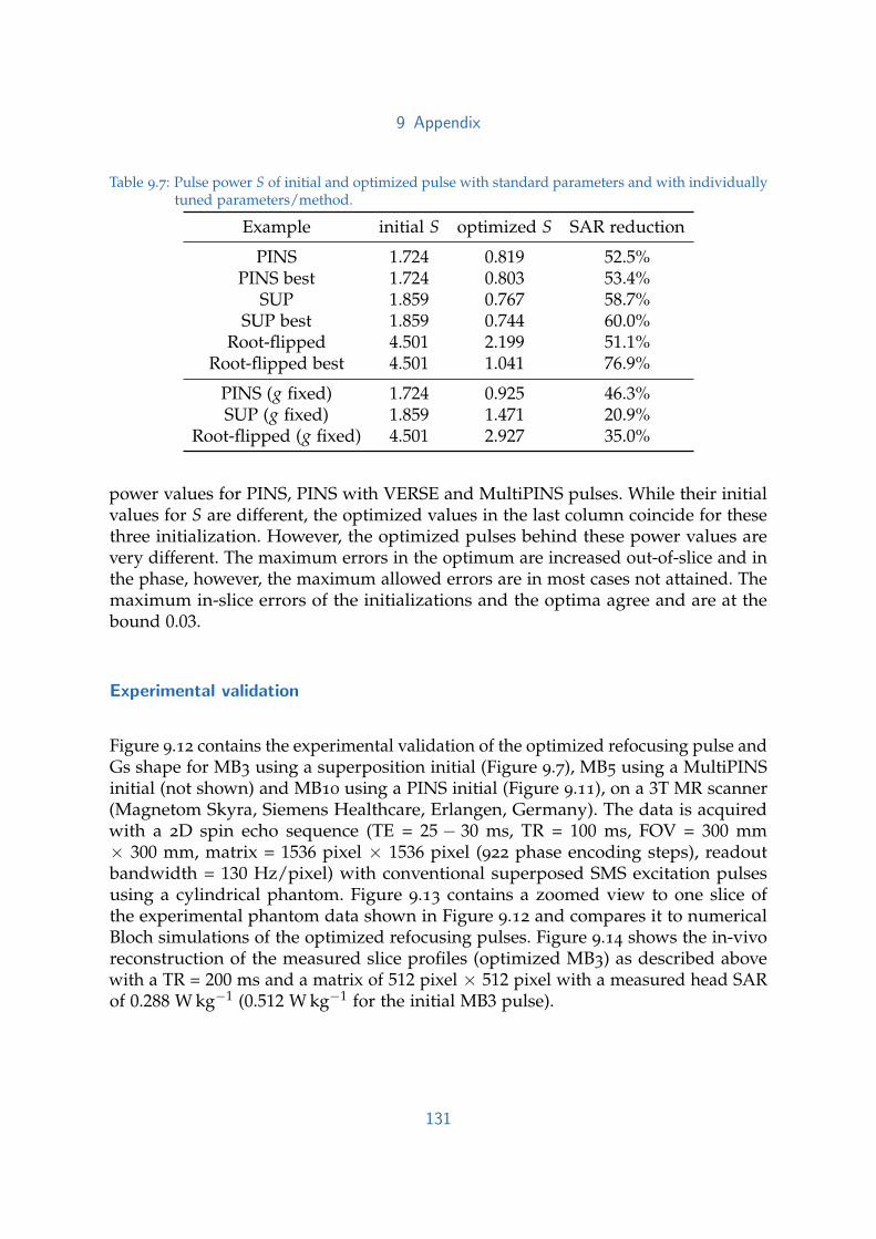
9 Appendix
Table 9.7: Pulse power S of initial and optimized pulse with standard parameters and with individuallytuned parameters/method.
Example initial S optimized S SAR reduction
PINS 1.724 0.819 52.5%PINS best 1.724 0.803 53.4%
SUP 1.859 0.767 58.7%SUP best 1.859 0.744 60.0%
Root-flipped 4.501 2.199 51.1%Root-flipped best 4.501 1.041 76.9%
PINS (g fixed) 1.724 0.925 46.3%SUP (g fixed) 1.859 1.471 20.9%
Root-flipped (g fixed) 4.501 2.927 35.0%
power values for PINS, PINS with VERSE and MultiPINS pulses. While their initialvalues for S are different, the optimized values in the last column coincide for thesethree initialization. However, the optimized pulses behind these power values arevery different. The maximum errors in the optimum are increased out-of-slice and inthe phase, however, the maximum allowed errors are in most cases not attained. Themaximum in-slice errors of the initializations and the optima agree and are at thebound 0.03.
Experimental validation
Figure 9.12 contains the experimental validation of the optimized refocusing pulse andGs shape for MB3 using a superposition initial (Figure 9.7), MB5 using a MultiPINSinitial (not shown) and MB10 using a PINS initial (Figure 9.11), on a 3T MR scanner(Magnetom Skyra, Siemens Healthcare, Erlangen, Germany). The data is acquiredwith a 2D spin echo sequence (TE = 25 − 30 ms, TR = 100 ms, FOV = 300 mm× 300 mm, matrix = 1536 pixel × 1536 pixel (922 phase encoding steps), readoutbandwidth = 130 Hz/pixel) with conventional superposed SMS excitation pulsesusing a cylindrical phantom. Figure 9.13 contains a zoomed view to one slice ofthe experimental phantom data shown in Figure 9.12 and compares it to numericalBloch simulations of the optimized refocusing pulses. Figure 9.14 shows the in-vivoreconstruction of the measured slice profiles (optimized MB3) as described abovewith a TR = 200 ms and a matrix of 512 pixel × 512 pixel with a measured head SARof 0.288 W kg−1 (0.512 W kg−1 for the initial MB3 pulse).
131

9 Appendix
time in ms
0 2 4 6 8 10
RF
in µ
T a
nd G
s in m
T/m
-10
0
10
20
time in ms
0 2 4 6 8 10
RF
in µ
T a
nd G
s in m
T/m
-10
0
10
20
distance in m
-0.06 -0.04 -0.02 0 0.02 0.04 0.06
refo
cusin
g p
rofile
0
0.5
1
distance in m
-0.06 -0.04 -0.02 0 0.02 0.04 0.06
refo
cusin
g p
rofile
0
0.5
1
distance in m ×10-3
-4 -2 0 2 4
refo
cusin
g p
rofile
0
0.5
1
distance in m ×10-3
-1 -0.5 0 0.5 1
phase a
ngle
-2
0
2
Figure 9.7: Optimization results and spin domain Bloch simulations for a MB3 pulse. Initial (Row 1)and optimized (Row 2) RF and Gs (Re(RF) in blue, Im(RF) in yellow and Gs in red) withrefocusing profile |bNt |2. Zoom of the central slice (black lines mark the in-slice/out-of-sliceerror tolerance) with phase angle(bNt) (not part of the optimization) for the optimizedpulse (Row 3).
time in ms
0 2 4 6 8
RF
in µ
T a
nd G
s in m
T/m
-10
0
10
20
time in ms
0 2 4 6 8
RF
in µ
T a
nd G
s in m
T/m
-10
0
10
20
distance in m
-0.03 -0.02 -0.01 0 0.01 0.02 0.03
refo
cusin
g p
rofile
0
0.5
1
distance in m
-0.03 -0.02 -0.01 0 0.01 0.02 0.03
refo
cusin
g p
rofile
0
0.5
1
distance in m
-0.022 -0.02 -0.018 -0.016 -0.014
refo
cusin
g p
rofile
0
0.5
1
distance in m
-0.02 -0.019 -0.018 -0.017 -0.016
phase a
ngle
-2
0
2
Figure 9.8: Optimization results and spin domain Bloch simulations for a MB6 pulse. Initial (Row 1)and optimized (Row 2) RF and Gs (Re(RF) in blue, Im(RF) in yellow and Gs in red) withrefocusing profile |bNt |2. Zoom of the central slice (black lines mark the in-slice/out-of-sliceerror tolerance) with phase angle(bNt) (not part of the optimization) for the optimizedpulse (Row 3)
132

9 Appendix
time in ms
0 2 4 6 8
RF
in
µT
-10
0
10
smax=
100
time in ms
0 2 4 6 8
RF
in
µT
-10
0
10
smax=
50
time in ms
0 2 4 6 8
RF
in
µT
-10
0
10
smax=
10
time in ms
0 2 4 6 8
Gs in
mT
/m
0
5
10
time in ms
0 2 4 6 8
Gs in
mT
/m
0
5
10
time in ms
0 2 4 6 8
Gs in
mT
/m
0
5
10
time in ms
0 2 4 6 8
sle
w r
ate
in
T/m
/s
-100
0
100
time in ms
0 2 4 6 8
sle
w r
ate
in
T/m
/s
-100
0
100
distance in m
0 2 4 6 8
sle
w r
ate
in
T/m
/s
-100
0
100
Figure 9.9: Optimized MB6 RF pulse (Re(RF) in blue, Im(RF) in red), slice-selective gradient Gs andgradient slew rate for different maximum values of s: smax ∈ 100, 50, 10 T m−1 s−1.
time in ms
0 1 2 3 4 5 6 7 8
RF
in
µT
an
d G
s in
mT
/m
-10
0
10
gmin=
2.3
time in ms
0 1 2 3 4 5 6 7 8
RF
in
µT
an
d G
s in
mT
/m
-10
0
10
gmin=
1
time in ms
0 1 2 3 4 5 6 7 8
RF
in
µT
an
d G
s in
mT
/m
-10
0
10
gmin=
0
Figure 9.10: Optimized MB6 RF pulse and slice-selective gradient shape (Re(RF) in blue, Im(RF) inyellow and Gs in red) for different minimal values of Gs: gmin ∈ 0, 1, 2.3 mT m−1.
133

9 Appendix
Table 9.8: Performance of the optimization method for different initializations for an MB5 example.Depicted are the maximum errors and the pulse power S both for the initial and optimizedpulse. The maximum errors were constrained by 0.03 in-slice , by 0.02 out-of-slice , and by0.01 in the phase constraint.
initial optimizedInitialization error error error max |B1| S error error error S S best
in-slice out-of-slice phase µT 10−5T2s in-slice out-of-slice phase 10−5T2s 10−5T2s
SUP 0.0318 0.0142 0.0031 18 1.9531 0.0300 0.0066 0.0100 0.7712 0.7677SUP VERSE 0.0297 0.0016 0.0010 14 1.4461 0.0300 0.0200 0.0032 0.5603 0.5556
PINS 0.0294 0.0010 0.0009 13 1.1301 0.0300 0.0116 0.0030 0.4163 0.4108PINS VERSE 0.0297 0.0014 0.0008 13 0.9967 0.0300 0.0146 0.0093 0.4578 0.4093MultiPINS 0.0297 0.0016 0.0009 8 0.7262 0.0300 0.0200 0.0032 0.4144 0.4127
9.2.5 Discussion
We presented a general framework for optimal control based joint design of RFpulses and gradient waveforms for MRI. The framework is flexible in the primaryoptimization goal, which was chosen as SAR reduction in the examples above, and inthe desired magnetization profile. The latter can range from a conventional singleslice in the isocenter, to asymmetric or off-resonance profiles, or SMS. While weincluded the most important inequality constraints for RF pulse design, it is possibleto add other constraints and treat them with the presented penalization method.Otherwise, constraints can also be turned off by choosing an infinite bound.
The examples were chosen in the context of SMS imaging, where the pulse powerand peak B1 amplitude are easily exceeded and complying the hardware constraintsis crucial for practical applications. Therefore, the optimal control method was testedin the numerical experiments focusing on SAR reduction of several SMS refocusingpulses for various slice thicknesses, time bandwidth products and a slice accelerationfactor ranging from MB3 to MB10. The initial pulses are designed with differentmethods, with conventional superposition[162], VERSE[112], [160], root flipping[173],PINS[131] and MultiPINS [179] with SLR based subpulses[66]. We investigated fourdifferent examples for low (MB3), intermediate (MB5 and MB6) and large (MB10)slice acceleration factors. PINS pulses for low MB factors and superposition pulses forlarge MB factors typically have a very long pulse duration. Therefore we chose to useMB3 superposition pulses for low and MB10 PINS pulses for large MB factors onlyand compare different initialization methods (SUP, SUP VERSE, PINS, PINS VERSEand MultiPINS) for the intermediate MB5 case. The root flipping pulse is excludedfrom this comparison and investigated separately for MB6 as it creates refocusingprofiles with a non linear phase.
134

9 Appendix
time in ms
0 2 4 6 8RF
in µ
T a
nd G
s in m
T/m
-20
0
20
time in ms
0 2 4 6 8RF
in µ
T a
nd G
s in m
T/m
-20
0
20
distance in m
-0.1 -0.05 0 0.05 0.1
refo
cusin
g p
rofile
0
0.5
1
distance in m
-0.1 -0.05 0 0.05 0.1
refo
cusin
g p
rofile
0
0.5
1
distance in m
-0.015 -0.014 -0.013 -0.012 -0.011 -0.01 -0.009
refo
cusin
g p
rofile
0
0.5
1
distance in m
-0.013 -0.0125 -0.012 -0.0115 -0.011
phase a
ngle
-2
0
2
Figure 9.11: Optimization results and spin domain Bloch simulations for a MB10 pulse. Initial (Row 1)and optimized (Row 2) RF and gradient waveform (Re(RF) in blue, Im(RF) in yellowand Gs in red) with refocusing profile |bNt |2. Zoom of the central slice (black lines markthe in-slice/out-of-slice error tolerance) with phase angle(bNt) for the optimized pulse(Row 3)
The results show that the proposed optimal control model and method can reducethe pulse power dramatically. The overall power of the initial pulses was reducedby roughly 58 percent for SUP MB3 and 52 percent for PINS MB10 (and by 77percent for the RF MB6 pulse with a higher tolerance ein and eout, see Tab. 9.3).Please note that the initial power of the PINS pulse already lies in the range ofthe MB3 pulse designed with superposition. As can be seen in the Figures 9.7-9.11
the optimal waveforms vary in their shape, and hence depend on the initialization.The figures show that the maximum and mean B1 amplitude is reduced and theslice-selective gradient is modulated. While the initial PINS already uses a timevarying Gs, the optimized superposition and in particular the optimized root flippedexample introduce fluctuating Gs curves from constant initializations. The extent ofthe fluctuations in Gs changes with the prescribed maximum gradient slew rate, seeFig.9.9, and small fluctuations give a slightly reduced but still significant reduction inthe pulse power, see Tab. 9.6. Even a constant and fixed Gs allows for a significantreduction of the pulse power for the root flipped initialization, but only a slightreduction for the superposition pulse, see Tab. 9.7. Keeping the non-constant Gs fromPINS initialization fixed allows for nearly the same reduction of the pulse power aswith the joint control. Accordingly, joint control is always beneficial, but the gainvarys with the specific examples.
135

9 Appendix
phanto
m (
MB
3)
distance in mm
-40 0 40
a.u
.
distance in mm
-3 0 3
a.u
.
distance in mm
-43 -40 -37
a.u
.
phanto
m (
MB
5)
distance in mm
-100 -50 0 50 100
a.u
.
distance in mm
-3 0 3
a.u
.
distance in mm
-103 -100 -97
a.u
.
phanto
m (
MB
10)
distance in mm
-100 -50 0 50 100
a.u
.
distance in mm
-15 -12 -9
a.u
.
distance in mm
-111 -108 -105
a.u
.
Figure 9.12: Reconstructed experimental data for the optimized MB3, MB5 and MB10 candidates.
136

9 Appendix
distance in mm
-4 0 4
a.u
.
MB3
distance in mm
-4 0 4
a.u
.
MB5
distance in mm
-16 -12 -8
a.u
.
MB10
Figure 9.13: Simulated refocusing profile (solid line) and experimental phantom data (crosses) of thephantom measurements shown in Figure 9.12 for MB3 (zoom to one slice).
in-v
ivo
Figure 9.14: Reconstructed experimental data for in-vivo measurements using the optimized MB3pulse.
137

9 Appendix
Five different initializations were compared for an intermediate MB factor of 5 witha uniform pulse duration and comparable error properties. The pulse power washeavily reduced in all cases while the maximal in-slice errors εin remained the same.An increase in the out-of-slice errors εout and phase errors εph was observed, but itremained below the prescribed error bounds of 2% and 0.01 radians, respectively.A superposition pulse with VERSE yielded S ≈ 0.56 and therefore outperformedthe same pulse without VERSE (S ≈ 0.77). However, much better power values ofS ≈ 0.41 were observed for optimized PINS, PINS with VERSE and MultiPINS pulses.Therefore, it seems that the optimal control method performs best with PINS basedinitializations, especially for large MB factors.
These improvements in the pulse power were possible by allowing a controlled deviationof 3% and 5% for the slice profile accuracy along with 2% and 4% for the out-of-slice region compared to an ideal rectangular refocusing with a transition zoneexcluded from the optimization. For two of the examples (SUP MB3 and PINS MB10)this formulation results in a slightly steeper refocusing profile for the optimizedrefocusing compared to the initial. Figures 9.7-9.11 show that the controlled deviationis not exceeded anywhere in the observation domain. In other words, the profileconstraints are fulfilled exactly, which is an achievement of the presented penalizationtechnique.
Two second-order methods of numerical optimal control were introduced, that bothuse adjoint-based exact discrete derivatives, also for the second derivative. The precisederivative information allows for better progress when approaching the minimizer.For robustness of the optimization method w.r.t. the initialization and the problemparameters we embedded the Newton-type method into a trust-region frameworkusing the Steihaug-CG method. Additionally, Steihaug-CG reduces the computationaleffort of Newton-type methods, since it saves many Hessian evaluations in the firstphase of the optimization. In the second phase of the optimization both methodsprofit from an increased convergence order compared to first-order methods. Tosave computational effort, both methods were applied as a Newton-Krylov methodwith a matrix-free evaluation of the Hessian. By semismooth Newton techniques theinequality constraints on the control variables were included into the optimizationwithout increasing the numerical effort. The parameters of the optimization methodwere adapted automatically, or calibrated in the numerical experiments shown above.With these parameters the semismooth quasi-Newton method yields good results inshort computational time. In contrast, the semismooth Newton method which usesincreased computation time gives the best results.
Two examples for turbo spin echo sequences included explicit phase constraints,whereas the two other examples, intended for double refocused diffusion sequences,did not constrain the phase of the refocusing profile. The influence of the phase
138

9 Appendix
constraints on the optimal solutions is less severe than expected and the optimizedcases lead to similar power reductions in the range of 50% for the standard constraints(Tab. 9.6).
The prescribed amplitude constraints on the optimized RF pulse, the gradient andits slew rate ensure practical applicability on MR scanners. Due to the semismoothNewton method as well as the penalization technique, all these constraints are neverexceeded in the optimum. More closely, the results show that the maximum valuesfor the B1 amplitude and gradient strength were not attained in the optimal solution.This is due to the fact, that the reduction of the pulse power and the boundaryconditions for the gradient already pull the maximum value downwards. However,both these constraints become active for examples with smaller maximum values,different boundary conditions, and especially for smaller pulse durations. In contrast,we observe that the slew rate constraint is active in any of the investigated scenarios,which can e.g. be seen in Fig. 9.9. A nonnegative minimum gradient value is alsoin effect for large pulse durations, as can be seen in Fig. 9.10. If the minimumgradient value gets too large, the possible reduction of the pulse power is decreasedsignificantly, as can be seen for gmin = 2.31 in Tab. 9.6.
The pulses were designed based on the spin-domain description neglecting therelaxation effects. To justify this simplification we performed full Bloch simulations[233] for the optimized pulses and compared the simulations to the spin-domainresults. The relaxation times were set to those of the cylindric phantom (T1 = 102ms, T2 = 81 ms) used in the experiment. In all simulations, the refocusing profiles ofthe optimized examples do not degenerate significantly in the presence of relaxation.We see a simple scaling of the refocusing profiles, similar to conventional RF pulsesfor short T2 values. The effects of T1 is an increase of the refocusing error outside ofthe slices, which is compensated by the T2 relaxation and remains below the alloweddeviation for each example. Since the T1 relaxation times of typical in-vivo tissueare even higher and their influence on the refocusing profiles are negligible. Thesefindings have been verified by the experimental phantom measurements.
The experimental validation was done on a 3T scanner exchanging the excitation andrefocusing pulse of a standard crushed spin echo sequence for a cylindrical phantom(MB3, MB5 and MB10) and in-vivo (MB3). Changing the readout gradient to the slicedirection allows for a direct measurement of the simultaneous excited and refocusedslices. The small inter slice ripples of the optimized refocusing pulses can be neglectedfor a real measurement as standard excitation pulses produce no marked transversalmagnetization at these inter slice positions and the refocused magnetization wouldbe weighted by a factor of sin(θ/2)2 with a spatially dependent but low inter slicerefocusing flip angle θ. Due to the adequate choice and implementation of the slewrate constraint, the fluctuating Gs shapes were implementable, and the measured slice
139

9 Appendix
profiles fit very well to the Bloch simulations for all measurements. The measuredwhole body SAR includes the non optimized excitation pulse and is therefore lowerthan the calculated power reduction of the optimized MB3 refocusing pulse. The goodaccordance of the simulations and the measurements shows the practical applicabilityof the optimized pulses on a standard clinical scanner. Using the specific hardwareconstraints of the desired MR system simplifies the application of optimized pulsessince no further modifications or transformations have to be done, that moreovercould reduce the optimality.
In simulations we compared the robustness of the optimized pulses w.r.t. inhomo-geneities in B0 and B1 to the one of the initial pulses. The initial pulse and gradientpairs have a constant k-space excitation velocity and constant B0 inhomogeneitieslead to a constant spatial shift. Despite the time varying slice-selective gradient ofthe optimized examples, which is known to be prone to off-resonance effects, theprofile fidelity remains almost unchanged in the range of ±500 Hz and the impactof the chemical shift (400 Hz at 3 T) is negligible. For applications with larger B0inhomogeneities, the minimal amplitude constraint of the slice selective gradient canbe increased or Gs can be fixed to enhance off-resonance robustness at the cost of adecreased power reduction. To investigate the influences of a temporal mismatch be-tween the RF and slice selective gradient and eddy currents on the refocusing profiles,Bloch simulations were performed using a temporal shift of the slice selective gradientshape with respect to the RF pulse (up to 10 µs) and a first order low pass filtering(normalized numerator and denominator of 0.5) of the slice selective gradient shape.Both effects led to a symmetric decrease of the refocusing efficiency in dependence ofthe distance to the isocenter. Compared to the used initials with constant or repetitivegradient functions, the fast changes in the optimized slice selective gradient are moreprone to these effects. However, such a behavior is not observable in the experimentalphantom measurements and leads to the conclusion that the optimized examples canbe successfully implemented on the used MR scanner without special compensationtechniques. To decrease the sensitivity of gradient imperfections of the optimizedresults, it should be possible to incorporate this directly in the optimization by enforc-ing a smoothness constraint on the slice selective gradient or to directly include thegradient impulse response[234]. In the context of B1 inhomogeneities all optimizedexamples behave similar as the initial pulses and lead to a smooth transition of higherand lower flip angles for a static B1 increase or reduction, respectively. Furthermore,we do not expect an additional proneness to small in-plane and through-plane motioncompared to conventional RF pulses. The same holds for movements between theexcitation and the read-out. However, to reduce the influences of motion artifacts itshould be considered to reduce the overall refocusing time.
If the pulse power is not the primary restriction, then the pulse duration can bedecreased instead while keeping the pulse power. The reduction of the refocusing
140

9 Appendix
time is of high importance in SMS imaging and was chosen to be the topic of the2015 ISMRM Challenge[4]. In this direction the next step is to minimize the pulseduration by time-optimal control [235] in order to find the shortest possible pulsesthat fulfill the given inequality constraints.
9.2.6 Conclusions
The modeling of the profile accuracy with inequality constraints together with acustomized solution method allows for the computation of optimal RF pulses andslice-selective gradients, that outperform other approaches in the performance index.Moreover, the usage of constrained optimization guarantees for practical applicabilityand a direct implementation in clinical MR sequences.
Acknowledgments
This work is partially funded by the Austrian Science Fund (FWF) in the context ofproject ”SFB F3209-18” (Mathematical Optimization and Applications in BiomedicalSciences). Partial support from BioTechMed-Graz and NAWI Graz is gratefullyacknowledged. The authors thank Christian Clason from the University of Duisburg-Essen for many fruitful discussions on the topic of the paper.
9.2.7 Lagrange calculus in the spin domain
The adjoint based derivative is set up using a real-valued Lagrangian together with theWirtinger calculus. Therefore we introduce the complex RF pulse Um = um + ivm =rmeiϑm . The Lagrange multipliers for the discrete Bloch equation (9.20) are calledpm, qm ∈ C for m = 1, . . . , Nt. The control constraints (9.24) are kept explicitely. TheLagrangian of the penalized problem is defined in the usual way depending on the
141

9 Appendix
control variables rm, ϑm, gm, the state variables am, bm and the Lagrange multiplierspm, qm as
L =τ
2
Nt
∑m=1
r2m + ζϑ2
m + ζg2m +
δµout
2p ∑zj∈Ωout
(|bNt |2
e
)p
+δµin
2p ∑zj∈Ωin
(|bNt |2 − 1
e
)p
+δµp
p
L
∑l=1
∑zj∈Sl
(ϕ− ϕl
ep
)p
+τµg
p
Nt
∑m=2
(gm − gm−1
τsmax
)p
− ∑zj∈Ω
Re Nt
∑m=1
(am − αmam−1 + β∗mbm−1) p∗m
+ (bm − βmam−1 − α∗mbm−1) q∗m
.
A compact form of the first-order necessary conditions can be derived efficientlyusing the Wirtinger calculus. In particular, for a Lagrangian of the form L = Re(LC)with a complex-valued expression LC the derivatives w.r.t the real and imaginarypart Z1, Z2 of a complex variable Z = Z1 + iZ2 can be combined to
∂L∂Z1
+ i∂L∂Z2
=∂LC
∂Z∗+
(∂LC
∂Z
)∗using the Wirtinger derivatives [229] of a function f : C→ C, Z = Z1 + iZ2 7→ f (Z)
∂ f∂Z
=12
(∂ f
∂Z1− i
∂ f∂Z2
),
∂ f∂Z∗
=12
(∂ f
∂Z1+ i
∂ f∂Z2
).
In our case LC does not depend on pm, qm, a∗m, b∗m. Therefore the state equations (9.20)are easily recovered by differentiation w.r.t. p∗m, q∗m. Analogously differentiating w.r.t.am and bm and complex conjugation gives the adjoint Bloch equations
pm = α∗m+1pm+1 + β∗m+1qm+1,qm = −βm+1pm+1 + αm+1qm+1,
142

9 Appendix
for m = 1, . . . , Nt − 1 and pointwise in each zj ∈ Ω. For the terminal condition incase of a refocusing pulse both Wirtinger derivatives w.r.t. bNt and b∗Nt
have to beevaluated. Depending on the location zj we find pNt = 0 and
qNt =µoutδ
eχΩout
(|bNt |2
e
)p−1
bNt
+µinδ
eχΩin
(|bNt |2 − 1
e
)p−1
bNt +
NMB
∑l=1
χSl
δµp
e[(ϕ− ϕl
ep
)p−1
− 1Nl
∑zk∈Sl
(ϕ(zk)− ϕl
ep(zk)
)p−1]
2ibNt
b∗NtbNt
.
The last fraction stems from the chain rule using the derivative of the arctan functionin ϕ = arg(b2
Nt). Moreover, χSl is the characteristic function of the in-slice set Sl =
zl1, . . . , zl
Nl with Nl points and mean phase ϕl = ∑Nl
k=1 ϕ(zlk)/Nl.
The gradient of the reduced objective j′ = Ex+ F′(x) is given by the partial derivativesw.r.t the control variables. Its components are given by chain rule for the polarcoordinates
∂L∂rm
= τrm +∂L∂um
cos(ϑm) +∂L∂vm
sin(ϑm),
∂L∂ϑm
= ζτϑm −∂L∂um
rm sin(ϑm) +∂L∂vm
rm cos(ϑm),
for m = 1, . . . , Nt and by ∂L∂gm
, m = 2, . . . , Nt − 1, which is computed below. Each firstterm is collected in Ex, and the other terms constitute F′(x). In these equations weneed
∂L∂um
= Re(
∂LC
∂Um+
∂LC
∂U∗m
),
∂L∂vm
= Im(
∂LC
∂U∗m− ∂LC
∂Um
).
With ∂α∗m∂φm
=(
∂αm∂φm
)∗and analogously for βm the result is
∂L∂um
=γ2τ2umRm − γτ Im(Qm), m = 1, . . . , Nt,
∂L∂vm
=γ2τ2vmRm − γτ Re(Qm), m = 1, . . . , Nt,
143

9 Appendix
with
Qm = ∑zj∈Ω
sin(φm/2)1
φm
(am−1q∗m − b∗m−1pm
),
Rm = ∑zj∈Ω
1φm
Re (
am−1p∗m + b∗m−1qm) ∂αm
∂φm
+(am−1q∗m − b∗m−1pm
) ∂βm
∂φm
,
∂αm
∂φm= i
γτzgm
φm
(cos(φm/2)
2− sin(φm/2)
φm
)− sin(φm/2)
2,
∂βm
∂φm= i
γτ(um + ivm)
φm
(cos(φm/2)
2− sin(φm/2)
φm
).
Differentiation w.r.t. gm gives finally
∂L∂gm
= ζτgm + ∑zj∈Ω
Re
(am−1p∗m + b∗m−1qm)
∂αm
∂gm
+ (am−1q∗m − b∗m−1pm)∂βm
∂gm
+µg
smax
(gm − gm−1
τsmax
)p−1
−µg
smax
(gm+1 − gm
τsmax
)p−1
,
for m = 2, . . . , Nt − 1 and with
∂αm
∂gm=
γτzφm
(i sin(φm/2) + γτzgm
∂αm
∂φm
),
∂βm
∂gm=
(γτz)2
φmgm
∂βm
∂φm.
144

9 Appendix
9.3 Simultaneous Multislice Refocusing via TimeOptimal Control
Armin Rund1,2,†, Christoph Stefan Aigner3,† Karl Kunisch1,2,4 and Rudolf Stoll-berger2,3
This is a preprint of the publication ”Simultaneous multislice refocusing via timeoptimal control”. Magnetic Resonance in Medicine, Early view: February 2018, doi:https://doi.org/10.1002/mrm.27124
Abstract
Purpose: Joint design of minimum duration RF pulses and slice-selective gradientshapes for MRI via time optimal control with strict physical constraints, and itsapplication to simultaneous multislice (SMS) imaging.Theory and Methods: The minimization of the pulse duration is cast as a time op-timal control problem with inequality constraints describing the refocusing qualityand physical constraints. It is solved with a bilevel method, where the pulse length isminimized in the upper level, and the constraints are satisfied in the lower level. Toaddress the inherent nonconvexity of the optimization problem, the upper level isenhanced with new heuristics for finding a near global optimizer based on a secondoptimization problem.Results: A large set of optimized examples shows an average temporal reduction of87.1% for double diffusion and 74% for turbo spin echo pulses compared to PINSpulses. The optimized results are validated on a 3T scanner with phantom measure-ments.Conclusion: The presented design method computes minimum duration RF pulseand slice-selective gradient shapes subject to physical constraints. The shorter pulseduration can be used to decrease the effective TE in existing EPI or echo spacing inTSE sequences.
1Institute for Mathematics and Scientific Computing, University of Graz, Heinrichstr. 36, 8010 Graz,Austria
2BioTechMed-Graz, 8010 Graz, Austria†Armin Rund and Christoph Stefan Aigner have contributed equally to the paper3Institute of Medical Engineering, Graz University of Technology, Stremayrgasse 16/III, 8010 Graz,Austria
4Johann Radon Institute for Computational and Applied Mathematics (RICAM), Austrian Academy ofSciences, Altenbergstraße 69, 4040 Linz, Austria
145
9 Appendix
9.3.1 Introduction
Simultaneous Multislice (SMS) imaging acquires the information of different slicessimultaneously to reduce the overall acquisition time and is an emerging imagingtechnique with various applications such as multi-directional diffusion tensor imag-ing [209], short echo time (TE) functional imaging [236] and clinically important turbospin echo (TSE) based sequences [195]. Contrary to pure in-plane accelerated parallelimaging, SMS acceleration in slice direction acquires signal for every extra slice mea-sured and has only a minimal signal-to-noise penalty [95]. Recently, the applicationof Wave-CAIPI [237], originally proposed for 3D encoding, to SMS imaging allowedan increase in the number of simultaneous slices, called the multiband (MB) factor, to13 without major g-factor penalties [195]. On the other hand, SMS refocusing pulseswith a low MB factor but a good refocusing profile are beneficial for high resolutiondiffusion imaging [173], [238], [239].
However, SMS imaging requires RF pulses that simultaneously excite or refocus slices,which typically result in RF amplitudes and power which are too high, or in verylong pulse durations [95]. Historically, the first SMS RF pulse design method is basedon a superposition of frequency shifted sub-pulses [162]. To overcome the limitationof a linear scaling of the B1 peak amplitude and overall RF power with the MB factor[95], [163], different groups proposed design methods via phase modulation [174],time shifted superposition [175], root-flipping [173] and use of the wavelet domain[178]. After the pulse design, additional B1 and power reduction can be achievedby applying variable-rate selective excitation (VERSE) [112], [160], [172]. However,high MB factors lead to a strong oscillation of the RF amplitude and a direct VERSEapplication might require additional smoothing of the otherwise too rapidly changinggradient waveform, which was resolved by applying VERSE on the overall RF pulseenvelope[176]. Alternatively, an inherent power reduction in the pulse design ispossible using the power independent number of slices (PINS) [131] method thatutilizes periodic excitation patterns, with the limitation that a low time-bandwidthproduct (TBP) is generally used in order to avoid long pulse durations.
The combination of PINS pulses with conventional SMS pulses, MultiPINS [179],combines both approaches to reduce the overall pulse duration and increase thebandwidth of PINS pulses.
In addition, SMS RF pulses can also be designed by optimal control methods. OptimalControl (OC) has proven to be successful in NMR and MRI to design accurateexcitation profiles based on different models such as the Liouville-von Neumannequation [155], [156], [158], the Bloch equations [1], [157], [184], [240], or the Blochspin-domain model [49].
146

9 Appendix
To encourage researchers to focus on new methods that compute short SMS pulseswith a low B1 peak and SAR, while achieving accurate excitation/refocusing profiles,SMS pulse design was chosen to be the topic of the 2015 ISMRM challenge [4] (October2015 to May 2016, http://challenge.ismrm.org/node/71). The method described inthis paper was developed and applied in its SMS design subchallenge.
In our preceding work [2], [241] we introduced an optimal control method for RFpulse design subject to different equality and inequality constraints using a fixedtime horizon. In contrast, we present here a new time optimal control modeling fordesigning RF pulses with minimum duration under technical constraints. Due to thefree terminal time, the solution of time optimal control problems [242] is algorithmi-cally involved and different methods are needed. We introduce a new bilevel methodwith time grid adaption and warm-start algorithms. Moreover, globalization plays acentral role, since both the free terminal time and the bilinear Bloch equation lead toa nonconvex optimization problem. Here, we introduce new heuristics for finding anear global optimizer. The optimization method is tested on 31 SMS refocusing exam-ples. The numerical results are validated by experimental phantom measurements ona 3T MR system.
9.3.2 Theory
In the following, refocusing in minimum time is posed as a time optimal control prob-lem with inequality constraints for slice profile fidelity and MR hardware restrictions.The constraints were inspired by the ISMRM Challenge [4].
Optimal control framework
We jointly optimize for the time horizon/pulse duration T, as well as the RF pulseand slice-selective gradient (Gs) slew rate values at each time sample. Applying anequidistant time grid tm = mτ, m = 0, . . . , Nt with step size τ = T/Nt, the RF pulseis described as B1,m = rm exp(iϑm) with amplitude rm, phase ϑm and the imaginaryunit i. The Gs amplitude gm is given via the slew rate sm as
gm = gm−1 + τsm−1, m = 2, . . . , Nt − 1 (9.35)
with given boundary conditions g1, gNt . The Bloch equation is solved exactly inthe spin-domain, see [66], [67], neglecting relaxation effects, which is reasonable
147
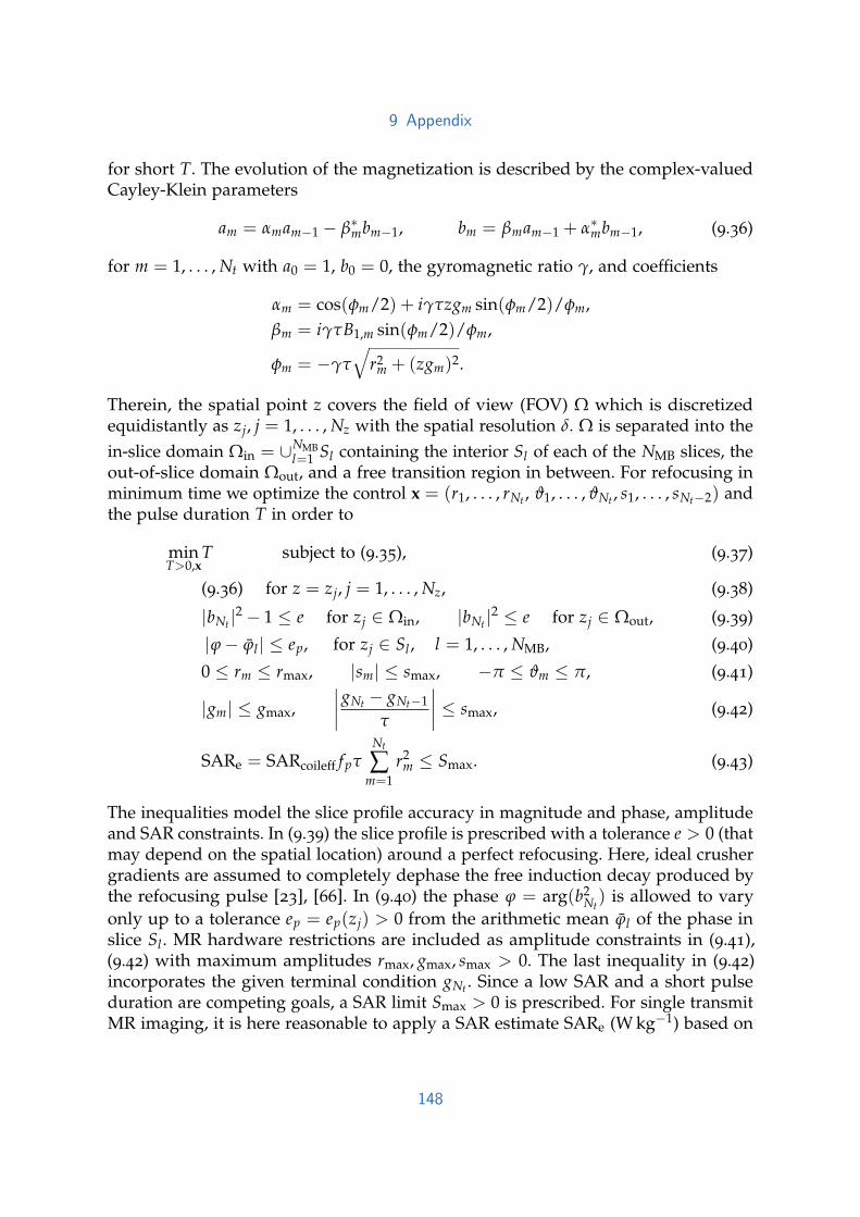
9 Appendix
for short T. The evolution of the magnetization is described by the complex-valuedCayley-Klein parameters
am = αmam−1 − β∗mbm−1, bm = βmam−1 + α∗mbm−1, (9.36)
for m = 1, . . . , Nt with a0 = 1, b0 = 0, the gyromagnetic ratio γ, and coefficients
αm = cos(φm/2) + iγτzgm sin(φm/2)/φm,βm = iγτB1,m sin(φm/2)/φm,
φm = −γτ√
r2m + (zgm)2.
Therein, the spatial point z covers the field of view (FOV) Ω which is discretizedequidistantly as zj, j = 1, . . . , Nz with the spatial resolution δ. Ω is separated into thein-slice domain Ωin = ∪NMB
l=1 Sl containing the interior Sl of each of the NMB slices, theout-of-slice domain Ωout, and a free transition region in between. For refocusing inminimum time we optimize the control x = (r1, . . . , rNt , ϑ1, . . . , ϑNt , s1, . . . , sNt−2) andthe pulse duration T in order to
minT>0,x
T subject to (9.35), (9.37)
(9.36) for z = zj, j = 1, . . . , Nz, (9.38)
|bNt |2 − 1 ≤ e for zj ∈ Ωin, |bNt |2 ≤ e for zj ∈ Ωout, (9.39)
|ϕ− ϕl| ≤ ep, for zj ∈ Sl, l = 1, . . . , NMB, (9.40)
0 ≤ rm ≤ rmax, |sm| ≤ smax, −π ≤ ϑm ≤ π, (9.41)
|gm| ≤ gmax,∣∣∣∣gNt − gNt−1
τ
∣∣∣∣ ≤ smax, (9.42)
SARe = SARcoileff fpτNt
∑m=1
r2m ≤ Smax. (9.43)
The inequalities model the slice profile accuracy in magnitude and phase, amplitudeand SAR constraints. In (9.39) the slice profile is prescribed with a tolerance e > 0 (thatmay depend on the spatial location) around a perfect refocusing. Here, ideal crushergradients are assumed to completely dephase the free induction decay produced bythe refocusing pulse [23], [66]. In (9.40) the phase ϕ = arg(b2
Nt) is allowed to vary
only up to a tolerance ep = ep(zj) > 0 from the arithmetic mean ϕl of the phase inslice Sl. MR hardware restrictions are included as amplitude constraints in (9.41),(9.42) with maximum amplitudes rmax, gmax, smax > 0. The last inequality in (9.42)incorporates the given terminal condition gNt . Since a low SAR and a short pulseduration are competing goals, a SAR limit Smax > 0 is prescribed. For single transmitMR imaging, it is here reasonable to apply a SAR estimate SARe (W kg−1) based on
148

9 Appendix
the global pulse power with constant SARcoileff (W/kg/µT2) and constant pulse ratefp.
This optimization problem is a pure time optimal control problem with controland state constraints. Such problems tend to possess bang-bang solutions, wherethe control constraint is active all the time but the value jumps between the upperand lower bound, see e.g. [242]. To approximate such optimal controls reliably wesuggest an L2-regularization of the controls with parameters α, ζ > 0. Furthermore,pointwise state-constrained optimal control problems are known to be involved sincethe Lagrange multiplier is irregular which leads to a decrease of the convergencespeed and accuracy of numerical solution methods, see e.g. [226]. To reduce theseeffects we apply the Lp-penalization of the state constraints from [2] and drive theexponent p → ∞ in a homotopy loop as we approach the optimizer. Therefore, wedefine the penalized objective
minT>0,x
J = T +τ
2
Nt
∑m=1
αr2m + ζϑ2
m +ζτ
2
Nt−2
∑m=1
s2m +
δµout
2p ∑zj∈Ωout
(|bNt |2
e
)p
+δµin
2p ∑zj∈Ωin
(|bNt |2 − 1
e
)p
+δµp
p
L
∑l=1
∑zj∈Sl
(ϕ− ϕl
ep
)p
+τµw
p
Nt−1
∑m=2
(gm
gmax
)p+
µT
p
(gNt − gNt−1
τsmax
)p(9.44)
with even number p and parameters µout, µin, µp, µw, µT > 0. α is automaticallyadapted to fulfill the SAR constraint (9.43), ζ is decreased as the optimizer is ap-proached. This penalized objective has to be minimized subject to (9.35), (9.36), (9.43),and the pointwise control constraints (9.41). For a fixed T this problem can be solvedwith established methods of numerical optimal control. We apply the trust-regionsemismooth quasi-Newton method from [2], which features robustness and adjoint-based exact discrete derivatives. It also handles the automatic adaption of the penaltyparameters µout, µin, µp, µw, µT. However, we still have to take care of the free terminaltime T.
Bilevel method for time optimal control
Time-optimal control problems can be solved by different approaches. In our ap-proach, the control x and T are separated in a bilevel method, where T is kept fixedin the lower level problem. Alternatively, both can be treated at once using timetransformations, see e.g. [243]. For the Bloch equation on equidistant time grids,
149

9 Appendix
numerical studies showed that a bilevel method prevails, since it facilitates keeping agood slice profile pattern after a time reduction. Furthermore, it offers more flexibilityin the time reduction, which is exploited for finding an improved minimizer.
The bilevel method is initialized using an existing method for SMS pulse design, e.g.conventional superposition [162], phase scrambling [174], root-flipped pulses [173],PINS [131] or MultiPINS [179]. Then, we alternately reduce the terminal time (upperlevel) and fulfill the constraints (lower level). For the former we keep the time stepconstant and reduce the terminal time by deleting one time point. The latter is doneby minimization of the penalized objective (9.44) for a fixed T using the trust-regionsemismooth quasi-Newton method of [2] with the following changes. First, we donot fully iterate until a relative or absolute stopping criteria is fulfilled, but terminateas soon as we have found an admissible solution to (9.39)–(9.43). Second, p is notchanged during the course of the semismooth quasi-Newton method, but altered inthe upper level of the bilevel method in order to have a monotonicity of p towardsthe optimum. Sometimes in the alternation of lower and upper level we decide toincrease p and might apply a refinement of the time grid (depending on the allowedraster time). The resulting bilevel method reads:
Step 1: Initialize control x0 and duration T0 with a conventional RF pulse designmethod, choose p and set n = 1.
Step 2: Upper level: Choose to delete one time instance tk applying the heuristicsfor an improved optimizer (9.45). Reduce the terminal time to Tn < Tn−1and warm-start xn = f (xn−1, k).
Step 3: Lower level: Minimize the penalized objective (9.44) for a fixed terminaltime Tn by a trust-region semismooth quasi-Newton method until anadmissible solution to the inequality constraints (9.39)–(9.43) is found. Theresulting control is xn.
Step 4: Decide to increase p, decrease ζ and/or to refine the time grid. Set n =n + 1 and repeat from Step 2.
Finally, we present the technical details of the time reduction. At deletion of a timepoint tk, the current control xn−1 is represented on the new time grid xn = f (xn−1, k)using a transfer function f that performs a good warm-start for the next lower leveloptimization. In particular, for maintaining a good slice profile this transfer functiondistributes the values of gk and the real and imaginary part of B1,k at the deletedtime instance tk symmetrically to the neighboring time instances. While doing so,we fulfill the constraints (9.41), (9.42). For technical details of f we refer to its sourcecode, which we published together with the software (see below). The time point tkto be deleted is chosen based on new heuristics for finding a near global optimizer.We choose the time point that allows the best performance after deletion, warm-start
150

9 Appendix
and Ng steps of the lower level solver. More precisely, the time tk is determined asthe global solution to the optimization problem
minm∈1,...,Nt
nJ(Tn, Q( f (xn−1, m))), (9.45)
where Q is an abstract function that stands for solving the lower level problem withthe trust-region semismooth quasi-Newton method of [2] in at most Ng iterations.Obviously, a larger Ng gives a better minimizer at the end, but increases the runtimeof the code. We use Ng = 0 for fast runs and 10 ≤ Ng ≤ 20 otherwise. Then theglobal minimizer of this auxiliary problem is computed exactly by total enumeration,or approximately by reusing information from previous upper level steps.
9.3.3 Methods
Simulations and pulse design
To test the general applicability of the proposed design method, we minimized thepulse duration in the test set of 31 cases given by the organizers of the ISMRMChallenge [4]. It contains different problem parameters (i.e. MB factor and slicethickness (THK)) and 13 different constraints (i.e. B1 peak, slew rate of Gs, maximumrefocusing errors and SAR limits). For the sake of completeness the most importantproblem parameters and constraints are repeated below. A full description is givenby the ISMRM 2015 challenge homepage and [4].
The maximum refocusing error e was set to 0.02 out-of-slice and 0.03 in-slice. Forthe design of all SMS refocusing pulses we assumed perfect crusher gradients. Thespace was discretized equidistantly with a resolution δ = THK/400. Two differentexample classes were considered for the optimization, double refocused diffusionand TSE/RARE imaging, each with different problem parameters (see SupportingTable S1). The global SAR constraint for all cases was set to be Smax = 3.2 W kg−1. TheSAR estimate SARe used an expected SAR efficiency of a 3T birdcage coil SARcoileffof 0.25 W/kg/µT2 and the assumed pulse rate fp for the two different scenarios (seeSupporting Table S1). The influence of amplitude constraints on the optimization wasanalyzed by using three different constraint settings given by actual hardware limits(see Supporting Table S2).
Diffusion pulses (DIFF). This example class asked for refocusing pulses for doublerefocused diffusion sequences [143] with a small MB factor (3–5) and THK (1–2mm), see Supporting Table S1. The number of spatial points Nz varied from 2401
151

9 Appendix
(MB = 3, THK = 2 mm) to 4801 (MB = 5, THK = 1 mm) to define a FOV of 120mm. The SAR estimate SARe used a repetition time (TR) of 120 ms with two identicalrefocusing pulses per repetition, resulting in a pulse rate fp = 16.67/s. The phase ofthe refocusing profile was not considered in the optimization.
Turbo spin echo pulses (TSE). Here the task was to generate SMS refocusing pulseswith a large number of simultaneous and thin slices (MB = 8–14, THK = 0.5–2mm, TBP = 3) for a repeated application in a TSE/RARE based sequence. A phaseconstraint with a maximal deviation of ep = 0.01 radiant from the mean phase perslice was added according to (9.40). The bigger FOV of 240 mm resulted in moredegrees of freedom in the spatial direction, ranging from 4801 (MB = 8, THK = 2mm) up to 19201 (MB = 14, THK = 0.5 mm). For all TSE cases a turbo factor of 12and a TR of 220 ms was assumed resulting in a pulse rate fp = 54.55/s.
The optimization was in general started from RF and Gs waveforms based on thePINS method [131]. The sub-pulse envelope was computed by the SLR algorithm [66]using d1 = e/4 (in-slice) and d2 = e/
√2 (out-of-slice). For τ = 10 µs the initial pulse
durations Tinit ranged from 8.710 ms (MB = 14, THK = 2 mm) to 32.42 ms (MB = 8,THK = 0.5 mm), see Table 9.9 and 9.10.
The optimization method was implemented in MATLAB (The MathWorks, Inc, Natick,USA). A version of it can be downloaded from https://github.com/rundar/mr.
control. Initially a small penalty exponent p = 6 was chosen, which was doubledtowards the optimum gradually to about 103 to 104 based on previous experience[2]. The trust-region semismooth quasi-Newton method [2] calibrated and adaptedthe other parameters in the objective (9.44) automatically. The time step size wasinitially set to τ = 10 µs, and gradually decreased by a factor of two as long asthe optimizer stayed below 20000 sampling points. For the challenge we typically
Table 9.9: Comparison of the optimized pulse duration (in ms) with the duration of the PINS initialguess for all DIFF examples.
MB3 MB4 MB5
THK PINS opt PINS opt PINS optmm ms ms ms ms ms ms
2.00 16.870 2.155 15.090 2.285 13.560 2.414
1.75 18.460 2.155 16.400 2.448 14.140 2.502
1.50 21.260 2.336 18.470 2.539 16.090 2.651
1.25 24.370 2.470 21.180 2.673 18.320 2.404
1.00 28.840 2.650 25.250 2.805 21.180 2.938
152

9 Appendix
chose Ng = 20 for the auxiliary optimization problem of the best time reduction,and reused the information several times. All calculations were done in parallel onthe high-performance-computing-cluster “RADON 1” (RICAM, Linz, Austria) usingone node (2× Xeon E5-2630v3 with in total 16 cores and 128 GB of RAM) for eachcase. Two examples were analyzed and described in more detail. One diffusion casewith MB = 3 and THK = 1.75 mm and one TSE/RARE case with MB = 12 andTHK = 1 mm.
Experiments
To validate the numerical simulations, phantom measurements were performed ona 3T MR scanner (Magnetom Skyra, Siemens Healthcare, Erlangen, Germany) us-ing the transmit/receive body-coil (birdcage). A standard crushed spin echo (SE)sequence was modified to import arbitrary RF and Gs shapes, and to measurethe slice profile by changing the phase encoding to the slice direction. We createdthree SE sequences, non-selective excitation and refocusing, slice-selective MB excita-tion with non-selective refocusing, and slice-selective MB excitation with optimizedslice-selective MB refocusing (applying the proposed optimization method). We im-plemented two optimized refocusing pulses and slice-selective gradient shapes, bothshown in Figure 9.17 (“scanner 2”), optimized for the hardware constraints thatcomply with the MR system used. Their durations were T = 3.38 ms (DIFF MB3) andT = 5.78 ms (TSE MB12) using a temporal grid of 10 µs equivalent to the gradientraster time of the MR system.
The utilized non-selective rectangular block pulses were 0.8 ms long for both, excita-tion and refocusing. The slice-selective MB excitation pulses were created applyingsuperposition with phase shifted SLR sub-pulse envelopes[66] resulting in a pulse
Table 9.10: Comparison of the optimized pulse duration (in ms) with the duration of the PINS initialguess for all TSE examples.
MB8 MB10 MB12 MB14
THK PINS opt PINS opt PINS opt PINS optmm ms ms ms ms ms ms ms ms
2.0 10.640 2.742 9.460 2.856 8.810 2.728 8.710 2.809
1.5 13.260 3.295 11.110 3.213 10.890 3.286 10.300 3.296
1.0 18.040 3.958 15.170 4.122 14.460 4.120 14.110 3.996
0.5 32.420 6.106 27.390 6.113 25.230 6.080 24.520 6.189
153

9 Appendix
time in ms
0 0.5 1 1.5 2 2.5 3
Gs in
mT
/m
0
20
40
60
time in ms
0 0.5 1 1.5 2 2.5 3
RF
in
µT
-20
-10
0
10
20
time in ms
0 0.5 1 1.5 2 2.5 3
sle
w r
ate
in
T/m
/s
-200
-100
0
100
200
distance in mm
-100 -50 0 50 100
refo
cu
sin
g p
rofile
0
0.5
1
distance in mm
-12 -10 -8
refo
cusin
g p
rofile
0
0.5
1
-110
angle
-2
0
2
-90 -70 -50 -30
distance in mm
-10 10 30 50 70 90 110
Figure 9.15: Optimization results and Bloch simulations for one representative TSE example. The firstrow shows the control variables B1 amplitude and slew rate of Gs for the refocusingduration of 3.16 ms. The second row depicts Gs shape, and the corresponding simulatedrefocusing profile |bNt |2. The last row shows a detail zoom of one slice to see the refocusingprofile together with the error corridor (black), and the phase angle arg(b2
Nt) per slice.
duration of T = 5.58 ms and a constant slice-selective gradient of 10 mT/m for theDIFF MB3 case. For the TSE MB12 case we have T = 10.92 ms and 5 mT/m.
The experiments were performed using a spherical phantom with a diameter of 240mm filled with 0.011 g MACROLEX blue per liter MARCOL-oil (T1 ≈ 200 ms andT2 ≈ 100 ms). High resolution data were acquired in the transversal plane with amatrix size of 1536× 1536 (1536 phase encoding steps) and a FOV of 300× 300 mmresulting in a voxel size of 0.2× 0.2 mm. For both cases we used TR = 300 ms. TheTE was set to 23 ms (DIFF MB3) and 30 ms (TSE MB12) for both the non-selective andoptimized SE experiments. The TE of the fully non-selective SE was set to 15.5 ms.All measurements were acquired after a manual shim with a sampling bandwidth of130 Hz and were repeated five times to compute the median with an increased signalto noise ratio. The experimental data using the optimized slice-selective refocusing
154

9 Appendix
were normalized by the fully non-selective SE measurement using a masked noisecut-off of 0.1.
9.3.4 Results
Below we present the results of our contribution to the ISMRM challenge. In particular,we show the real-valued RF pulses (B1,m ∈ R for all times) which were submitted forthe challenge.
Simulations
Supporting Figure S1 summarizes the numerical results of an optimized diffusionexample to refocus 5 slices with a thickness of 1.25 mm equally distributed overa FOV of 120 mm at a temporal resolution of τ = 0.625 µs. The overall terminaltime could be reduced to 2.404 ms, which is a reduction of 86.9% compared to theinitial PINS pulse with 18.32 ms and a reduction of 90.3% compared to a validpulse candidate based on conventional superposition with 24.85 ms (not shown). Theoptimized RF amplitude and slew rate are given in the first row of Supporting FigureS1. The second row additionally shows the Gs shape, and the simulated refocusingprofile for the whole FOV. A zoomed image in the third row shows, that the profilealways remains inside the black error corridor. The last plot shows the phase of eachrefocusing profile, which was not constrained here.
Figure 9.15 shows the analogous plots, this time for the optimized TSE refocusing(MB12, THK= 1 mm, FOC= 240 mm, τ = 0.625 µs). The optimization was done herewithout a constraint on the SAR. The pulse duration was reduced by 75% from 12.92ms to 3.16 ms compared to the initial PINS pulse. Again, the gradient amplitudein the third plot shows a large hump at the beginning and the end, and a smallzigzagging in between that remained from the initial PINS pulse. The slice profilefulfills the constraints, with an equiripple error in the out-of-slice region, which canbe seen in the zoomed plot in the third row for one slice. The last plot shows theadditional phase constraint for the TSE/RARE examples. The refocusing phase isnearly constant per slice, but each slice shows a different mean phase.
A summary for the total pulse duration of the PINS based initial guesses Tinitcompared to the time optimal pulse durations T is given in Table 9.9 (DIFF) andTable 9.10 (TSE). Here, all 31 examples were solved with the SAR constraint. Theachieved temporal reduction for the diffusion example is 86.9% (from 18.32 ms to
155
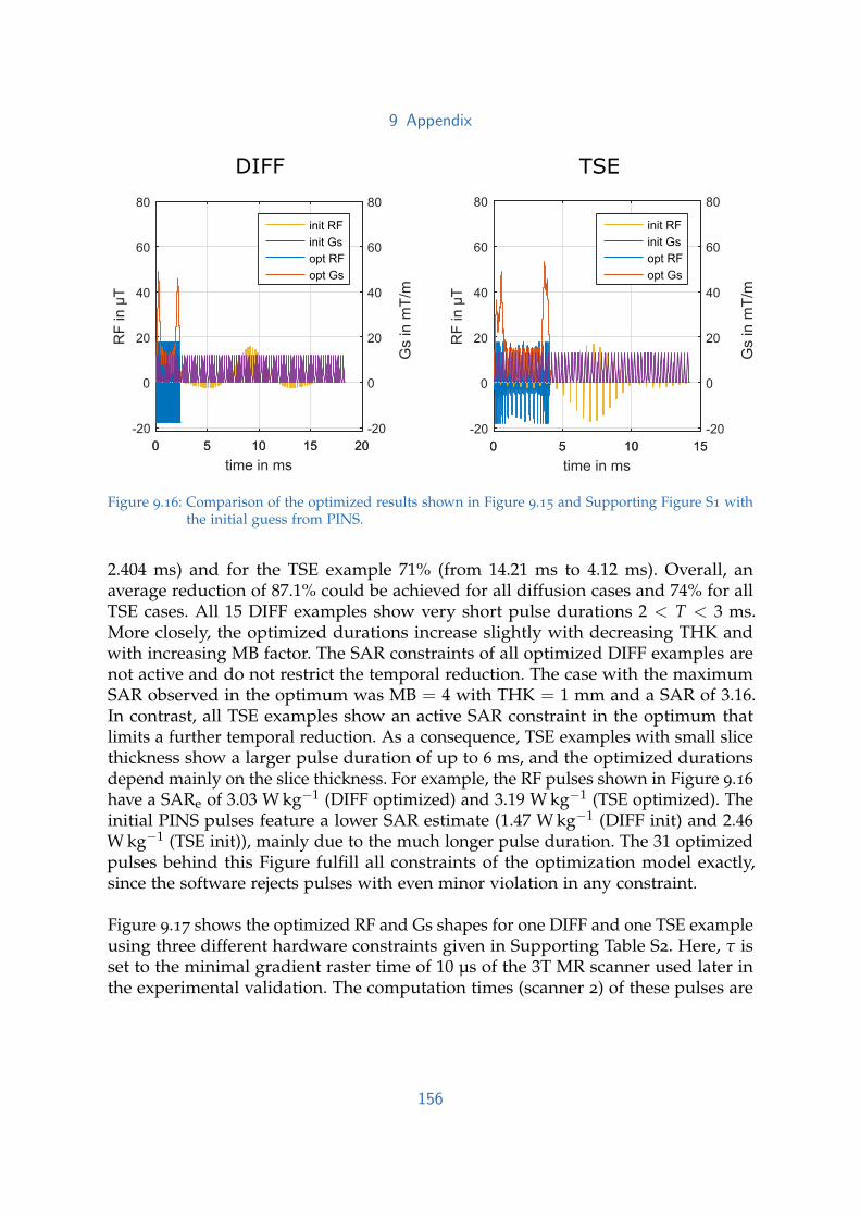
9 Appendix
DIFF
Gs in
mT
/m
time in ms
0 5 10 15R
F in µ
T
-20
0
20
40
60
80
init RF
init Gs
opt RF
opt Gs
0 5 10 15
-20
0
20
40
60
80
time in ms
0 5 10 15 20
RF
in
µT
-20
0
20
40
60
80
init RF
init Gs
opt RF
opt Gs
0 5 10 15 20
-20
0
20
40
60
80
TSE
Gs in
mT
/m
Figure 9.16: Comparison of the optimized results shown in Figure 9.15 and Supporting Figure S1 withthe initial guess from PINS.
2.404 ms) and for the TSE example 71% (from 14.21 ms to 4.12 ms). Overall, anaverage reduction of 87.1% could be achieved for all diffusion cases and 74% for allTSE cases. All 15 DIFF examples show very short pulse durations 2 < T < 3 ms.More closely, the optimized durations increase slightly with decreasing THK andwith increasing MB factor. The SAR constraints of all optimized DIFF examples arenot active and do not restrict the temporal reduction. The case with the maximumSAR observed in the optimum was MB = 4 with THK = 1 mm and a SAR of 3.16.In contrast, all TSE examples show an active SAR constraint in the optimum thatlimits a further temporal reduction. As a consequence, TSE examples with small slicethickness show a larger pulse duration of up to 6 ms, and the optimized durationsdepend mainly on the slice thickness. For example, the RF pulses shown in Figure 9.16
have a SARe of 3.03 W kg−1 (DIFF optimized) and 3.19 W kg−1 (TSE optimized). Theinitial PINS pulses feature a lower SAR estimate (1.47 W kg−1 (DIFF init) and 2.46W kg−1 (TSE init)), mainly due to the much longer pulse duration. The 31 optimizedpulses behind this Figure fulfill all constraints of the optimization model exactly,since the software rejects pulses with even minor violation in any constraint.
Figure 9.17 shows the optimized RF and Gs shapes for one DIFF and one TSE exampleusing three different hardware constraints given in Supporting Table S2. Here, τ isset to the minimal gradient raster time of 10 µs of the 3T MR scanner used later inthe experimental validation. The computation times (scanner 2) of these pulses are
156

9 Appendix
time in ms
0 1 2
DIF
F s
cenario
RF
in µ
T a
nd G
s in m
T/m
-20
0
20
40
60
80ISMRM challenge
RF
Gs
time in ms
0 0.5 1 1.5 2R
F in µ
T a
nd G
s in m
T/m
-20
0
20
40
60
80scanner 1
RF
Gs
time in ms
0 1 2 3
RF
in µ
T a
nd G
s in m
T/m
-20
0
20
40
60
80scanner 2
RF
Gs
time in ms
0 2 4
TS
E s
cenario
RF
in µ
T a
nd G
s in m
T/m
-20
0
20
40
60
80
RF
Gs
time in ms
0 2 4
RF
in µ
T a
nd G
s in m
T/m
-20
0
20
40
60
80
RF
Gs
time in ms
0 2 4R
F in µ
T a
nd G
s in m
T/m
-20
0
20
40
60
80
RF
Gs
Figure 9.17: Optimized RF and Gs shapes for different hardware constraints (shown dotted) summa-rized in Supporting Table S2 (left: ISMRM challenge, middle: scanner 1, right: scanner 2)and a fixed temporal resolution of 10 µs. The upper row shows a DIFF pulse for 3 sliceswith a thickness of 1.75 mm and the lower row shows a TSE pulse for 12 slices with athickness of 1 mm.
approximately 2h (DIFF) and 2.5h (TSE) using MPI on the hardware (16 CPU cores)described above.
Next, we investigated the influence of time-invariant B0 and B1 inhomogeneities onthe two optimized pulses shown in Figure 9.15 and Supporting Figure S1. Blochsimulations were performed with an off-resonance range of pm200 Hz and a B1variation of 75− 125%. The results for the optimized pulses and the correspondinginitial PINS pulse are depicted in Supporting Figure S2.
The optimized results do not change significantly w.r.t. the time resolution of thePINS initial guess or the initialization of the objective parameters, as long as thefinal time sampling rate is the same. In contrast, a coarser time discretization atthe end generally leads to an increased pulse duration. For instance, the shortestdiffusion candidate in Figure 9.17 optimized for a temporal discretization of τ = 10
157

9 Appendix
Figure 9.18: Reconstructed experimental spin echo data using a spherical oil phantom. Three differentpairings are used: non-selective excitation and refocusing (left), slice-selective MB12excitation and non-selective refocusing (middle), and slice-selective MB12 excitation andoptimized refocusing (right). The intersection is shown in Figure 9.19 in detail.
µs is about 17% longer (T = 2.61 ms) than the optimized candidate with a temporaldiscretization of 0.625 µs shown in Table 9.9 with T = 2.155 ms.
Experiments
Figure 9.18 shows the image reconstructions (magnitude) of the three SE experimentsusing a spherical oil phantom in the above mentioned 3T MR scanner. The optimizedrefocusing is based on the RF and Gs shapes of Figure 9.17 (“scanner 2”). Themeasured and reconstructed magnitude signal along the blue intersection line isplotted in detail in Figure 9.19 for the two slice-selective SE experiments.
There, the first and third row show the median of the high resolution DIFF and TSEphantom measurements, whereas the second, fourth and fifth row display zoomedimages of the slices displaying both the median (solid) and the measurements points(crosses). The median is computed out of five individual measurements with minornoise variations. There is a good agreement between the different SE experiments witha small signal reduction for the outermost OC TSE slices, visible in the lowest rightplot of Figure 9.19. The larger span in slice direction of the TSE example (240 mm)led to a comparable slice shift for both, the non-selective and optimized refocuseddata.
Figure 9.20 shows the intersection of the optimized SE experiment (median) normal-ized by the median of the non-selective SE experiment (shown for TSE in Figure
158
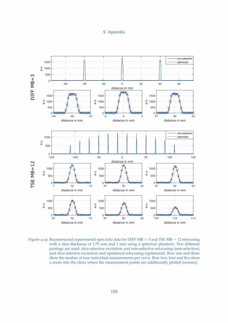
9 Appendix
distance in mm
-150 -100 -50 0 50 100 150
a.u
.
0
500
1000
non-selective
optimized
distance in mm
7 10 13
a.u
.
0
500
1000
distance in mm
27 30 33
a.u
.
0
500
1000
distance in mm
47 50 53
a.u
.
0
500
1000
distance in mm
67 70 73
a.u
.
0
500
1000
distance in mm
87 90 93
a.u
.
0
500
1000
distance in mm
107 110 113
a.u
.
0
500
1000
distance in mm
-60 -40 -20 0 20 40 60
a.u
.
0
500
1000
1500
non-selective
optimized
distance in mm
-43 -40 -37
a.u
.
0
500
1000
1500
distance in mm
-3 0 3
a.u
.
0
500
1000
1500
distance in mm
37 40 43
a.u
.
0
500
1000
1500
TSE M
B=
12
DIFF M
B=
3
Figure 9.19: Reconstructed experimental spin echo data for DIFF MB = 3 and TSE MB = 12 refocusingwith a slice thickness of 1.75 mm and 1 mm using a spherical phantom. Two differentpairings are used: slice-selective excitation and non-selective refocusing (non-selective),and slice-selective excitation and optimized refocusing (optimized). Row one and threeshow the median of four individual measurements per curve. Row two, four and five showa zoom into the slices where the measurement points are additionally plotted (crosses).
159

9 Appendix
distance in mm
-43 -40 -37
a.u
.
distance in mm
-3 0 3
a.u
.
distance in mm
37 40 43
a.u
.
exp
sim
distance in mm
7 10 13
a.u
.
distance in mm
27 30 33
a.u
.
distance in mm
47 50 53
a.u
.
distance in mm
67 70 73
a.u
.
distance in mm
87 90 93
a.u
.
distance in mm
107 110 113
a.u
.TSE M
B=
12
DIFF M
B=
3
Figure 9.20: Comparison of the experimental data (exp) with optimized refocusing normalized by afully non-selective SE measurement and the Bloch simulations (sim) for slice-selectiveexcitation and optimized DIFF MB = 3 and TSE MB = 12 refocusing.
160

9 Appendix
9.18). This normalization corrects for spatial B1 transmit/receive and signal variationsresulting from the spherical phantom. The normalized data points were comparedto the numerical Bloch simulations of the used excitation and optimized refocusing(solid).
9.3.5 Discussion
In addition to strict hardware and safety constraints, the minimal excitation orrefocusing duration is a critical and important parameter. Specifically in the contextof SMS imaging, RF pulses tend to have unacceptable long pulse durations limitingthe applications and capabilities of SMS imaging. This work presented a time optimalcontrol method, that, together with constrained optimization [2], can be applied todrastically reduce the pulse duration of SMS refocusing pulses while still fulfillingthe hardware constraints and slice profile accuracy. The methods were tested on the31 examples of the ISMRM Challenge on RF pulse design [4]. Compared to the giveninitialization of the ISMRM challenge (conventional superposed frequency shiftedcandidates for the diffusion cases, PINS for the TSE cases) the sum of the pulsedurations for the 31 examples was reduced from 520.4 ms down to 102.4 ms, whichis a reduction of 80.3%.
The proposed time optimal control method was tested for different problem parame-ters (Supporting Table S1) and constraints (Supporting Table S2). It robustly deliveredpulses that exploit the allowed error bands to significantly shorten the pulse duration.This robustness w.r.t. the parameters and initializations is a consequence of usinga trust-region globalization of the Newton-type method in the lower level problem.During the Challenge we tested the optimizer on different initializations computed byfrequency shifted superposition, phase modulation and PINS. In all cases the pulseswere shortened significantly. The shortest pulse durations were in most cases obtainedfor PINS based initial pulses, however, other educated guesses may outperform thepresented results. We note that different initializations can be tested by the user inthe published software.
The simulations of the optimized SMS pulses show accurate refocusing profileswith errors below the prescribed error bounds. Both, the treatment of the controlconstraints (i.e. peak B1 amplitude and the peak slew rate of Gs) by a semismoothquasi-Newton method and the treatment of the state constraints (profile accuracy,phase constraints, amplitude of Gs) by an Lp penalization with an iteratively increasedp → ∞ allowed for full exploitation of the inequality constraints [2]. The precisederivative information (exact discrete derivatives using adjoint calculus, second-order
161

9 Appendix
method) enabled additional progress in reducing the pulse duration, when many ofthe constraints were already active. In contrast to the SAR minimization for fixedpulse duration in [2] the RF amplitude constraint is much more important in thetime optimal case. In particular, the optimized controls in Figure 9.15 and SupportingFigure S1 show that (if the SAR and peak gradient constraint are not active) all theconstraints are active wherever it is possible, resulting in equiripple error distributionsand bang-bang controls. This is a typical behavior of solutions of pure time optimalcontrol problems, and it underlines the local optimality of the presented results. Withstronger constraints on the SAR or the peak gradient amplitude, optimized durationsincrease. In this case the optimal RF amplitude is at its bounds only in certain pointsduring the time interval, see Figure 9.17.
In all examples, the pulse duration can be further decreased by a temporal refinementat the cost of an increased computational effort. For example the diffusion case shownin Figure 9.17 yielded a minimum pulse duration of 2.61 ms for a typical time grid(τ = 10 µs) and of 2.155 ms after four further refinement steps (τ = 2.5 µs). For theSE measurements the temporal refinement was done only up to the minimal gradientraster time of the particular MR scanner.
All optimized examples are designed and evaluated for a distinct FOV. We wouldlike to mention here that both the PINS initial and optimized pulses create refocusingslices outside the FOV of interest. If this is unacceptable, the use of different initialguesses such as superposition pulses allows to increase the FOV and further restrictsthe refocusing profiles.
Optimized pulse durations of under 3 ms were observed throughout all diffusionexamples, see Table 9.9. Here, the SAR was never at its bounds, mainly because of thelow pulse rate. The maximum amplitude gmax for the Gs amplitude was only reachedin 3 of the 15 examples. In contrast, all optimized RF amplitudes and gradient slewrates were at their bounds almost everywhere with small exceptions around the twotime points of maximum gradient amplitude.
For the TSE examples, the initial PINS pulses already combine a good refocusingprofile with a small RF power that is exploited in the temporal reduction. Due to ahigher pulse rate, the SAR constraint has a strong influence on the pulse durationhere and is the main limiting factor for the temporal reduction. All 16 cases showan active SAR constraint in the optimum and outperform the initial PINS pulsesin terms of the required refocusing duration. For the case given in Figure 9.15, theoptimizer computes an admissible pulse candidate with a minimal pulse duration of3.155 ms without a SAR constraint, compared to 4.120 ms with a SAR constraint, seeFigure 9.16 and Table 9.10, of 3.2 W kg−1 - a factor of roughly 25%. This results in lessexploited RF shape where the RF envelope differs from the block shape of examples
162
9 Appendix
without an active power constraint, e.g. the DIFF MB5 case shown in Figure 9.16. Asa consequence of the active SAR constraint, the minimum durations turn out to beindependent of the MB factor, see Table 9.10. Instead, they mainly depend on the slicethickness.
In total we applied the proposed optimization method to design SMS refocusingpulses with a wide range of MB factors (3–14) and THK (0.5–2 mm). All optimizedpulses show a dramatically reduced pulse duration, on average by 87.1% for thediffusion and by 74.5% for the TSE examples, which allows significant reduction ofthe minimal TE of both, diffusion and TSE/RARE sequences.
Compared to state-of-the-art minimum duration design methods such as root-flipdesign [173], the achieved reduction of the proposed method is still significantlyhigher. For instance, the DIFF pulse used in the experiment (see Figure 9.17) is 57.4%shorter than a root-flipped pulse (T = 6.11 ms) designed with equivalent designparameters (512 time-points with τ = 11.93 µs, MB = 3, TBP = 4, THK = 1.75 mm,rmax = 12.5 µT and a refocusing error of 0.02 out-of-slice and 0.03 in-slice).
Comparison of DIFF examples without a distinct phase constraint with the TSEexamples designed with a pointwise phase constraint of the refocusing slices revealedthat the additional constraint only has a minor effect on the overall pulse duration.Although this is not shown in this work, the phase constraint can obviously bechanged to treat all slices at once to comply with the CPMG condition [244], [245].
With the current CPU based MPI implementation the pulses need to be precomputedand provided on the MR scanner. To reduce the current computation time, a speed-upof a factor 31 has been reported by using GPU parallelization[159]. Both optimizedSE measurements were in a good accordance with the non-selective refocusing.
For comparison of simulated and measured slice profiles, the transmit/receive sen-sitivity variations and spatial signal differences arising from the used spherical oilphantom were removed by normalization of the measurements with a fully non-selective SE reference scan. Then, comparisons between the normalized slice profileswith optimized refocusing and the Bloch simulations were performed (Figure 9.20).
In general, rapidly-varying RF pulses can be distorted by the limited bandwidth ofthe RF system[246]. To reduce this RF distortion, we design real valued RF pulsesthat are less prone to RF distortions[111]. Additionally we used a time grid of 10 µs,400 times the minimal RF duration of 25 ns. Therefore we do not expect significantalterations of the RF chain on the optimized RF shapes. This is supported by themeasured slice profiles. The question, whether time-optimal complex-valued RFpulses can outperform the real-valued ones will be part of future work. For systemswith different RF specifications or for the optimization of complex RF pulses, an
163

9 Appendix
additional constraint on the RF slew rate, analogous to the presented Gs slew rateconstraint, could be included in the optimization.
The question arises how the optimized pulses perform in the presence of gradientimperfections. Besides an identical slice shift for both refocusing examples (seeFigure 9.19) the slices of the optimized refocusing are attenuated with the distance tothe isocenter. After a manual shim there are only minor B0 inhomogeneities in thephantom and the slice shift mainly results from non-linear gradients at the boundaryof the field of view. The minor signal attenuations of the outermost slices are likelycaused by gradient distortions [115], [118]. The inclusion of gradient and amplifierimperfections for different MR systems in the optimization will be future work.
An additional gradient echo phase scan (not shown) showed a slightly asymmetric B0field that explains spatial signal differences between data from non-selective excitationand data from slice-selective excitation. However, these residual B0 inhomogeneitiesare not strong enough to explain the observed signal loss. The robustness of theoptimized pulses w.r.t. B0 and B1 inhomogeneities was investigated in simulations incomparison to the initial pulses (Supporting Figure S2). In general the slice displace-ment for both optimized cases are lower compared with the initial PINS pulses. Thisis mainly due to the heavily decreased pulse duration which reduces the B0 sensitivity.Due to a variable k-space velocity of the optimized examples, the refocusing profilesare thinned out with increasing off-resonance, but remain stable below pm100 Hz. Inthe context of B1 inhomogeneities, all examples share the principle that the thicknessof the refocusing profile is broadened for lower B1 scaling and thinned out for ahigher B1 scaling similar to other studies [247]. Depending on the application, aninclusion of B0/B1 robustness into the optimization framework will be focus of futurework.
9.3.6 Conclusions
The proposed time optimal design method yields optimized SMS refocusing pulsesfor clinical sequences with very short pulse durations with respect to representativephysical constraints given by current scanner hardware. The time optimal refocusingpulses will be beneficial for a broad range of SMS applications such as diffusion andspin echo based sequences to reduce the echo spacing and increase the signal qualityin terms of amplitude and robustness to motion.
164

9 Appendix
Acknowledgments
Partial support from ”SFB F32-N18” and BioTechMed-Graz are gratefully acknowl-edged. This work was in part supported by the ERC advanced grant 668998 (OCLOC)under the EU’s H2020 research program. The authors thank Christian Clason fromthe University of Duisburg-Essen for many fruitful discussions on the topic of thepaper.
165
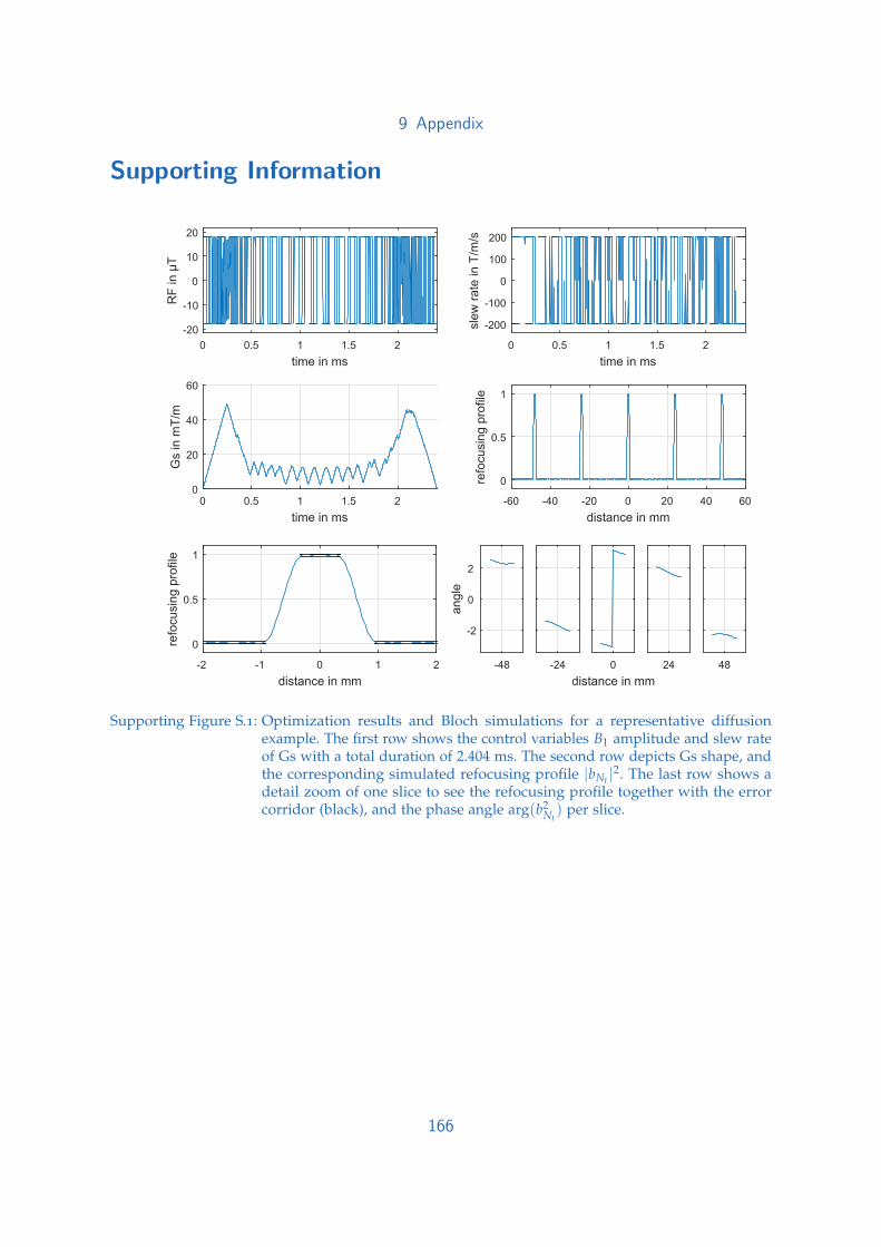
9 Appendix
Supporting Information
time in ms
0 0.5 1 1.5 2
Gs in m
T/m
0
20
40
60
time in ms
0 0.5 1 1.5 2
RF
in µ
T
-20
-10
0
10
20
time in ms
0 0.5 1 1.5 2
sle
w r
ate
in T
/m/s
-200
-100
0
100
200
distance in mm
-60 -40 -20 0 20 40 60
refo
cusin
g p
rofile
0
0.5
1
distance in mm
-2 -1 0 1 2
refo
cusin
g p
rofile
0
0.5
1
-48
angle
-2
0
2
-24
distance in mm
0 24 48
Supporting Figure S.1: Optimization results and Bloch simulations for a representative diffusionexample. The first row shows the control variables B1 amplitude and slew rateof Gs with a total duration of 2.404 ms. The second row depicts Gs shape, andthe corresponding simulated refocusing profile |bNt |2. The last row shows adetail zoom of one slice to see the refocusing profile together with the errorcorridor (black), and the phase angle arg(b2
Nt) per slice.
166

9 Appendix
distance in mm
108 110 112
B1
sca
ling
0.8
0.9
1
1.1
1.2
0
0.5
1
distance in mm
108 110 112
B0
off
res in
Hz
-200
-100
0
100
200
0
0.5
1
distance in mm
108 110 112
B1
sca
ling
0.8
0.9
1
1.1
1.2
0
0.5
1
distance in mm
108 110 112
B0
off
res in
Hz
-200
-100
0
100
200
0
0.5
1
TS
E s
cenario
distance in mm
45 46 47 48 49 50 51
B1
sca
ling
0.8
0.9
1
1.1
1.2
0
0.5
1
distance in mm
45 46 47 48 49 50 51
B0
off
res in
Hz
-200
-100
0
100
200
0
0.5
1
distance in mm
45 46 47 48 49 50 51
B1
sca
ling
0.8
0.9
1
1.1
1.2
0
0.5
1
distance in mm
45 46 47 48 49 50 51
B0
off
res in
Hz
-200
-100
0
100
200
0
0.5
1
DIF
F s
cenario
Supporting Figure S.2: Simulated refocusing profiles |bNt |2 (zoom to the outermost slice with com-parable refocusing profiles across all individual slices) for a variation in theoff-resonance and B1 inhomogeneity for four different pulses: the PINS-basedinitial pulses (first and third row) and the optimized pulses shown in Support-ing Figure S1 (second row) and Figure 1 (fourth row), respectively.
167

9 Appendix
Supporting Table S.1: Overview of the problem parameters for TSE and diffusion (DIFF).
MB factor FOV THK TBP fp phase[a.u.] mm mm [a.u.] 1/s [a.u.]
TSE 8 : 2 : 14 240 0.5 : 0.5 : 2.0 3 54.55 constantDIFF 3 : 1 : 5 120 1.0 : 0.25 : 2.0 4 16.67 free
Supporting Table S.2: Overview of the physical constraints used in the optimization.
gmax smax rmaxmT/m mT/m/ms µT
ISMRM challenge 80.0 200 18.0scanner 1 34.0 200 18.0scanner 2 24.0 180 12.5
168
Bibliography
[1] C. S. Aigner, C. Clason, A. Rund, and R. Stollberger, “Efficient high-resolutionRF pulse design applied to simultaneous multi-slice excitation”, J Magn Reson,vol. 263, pp. 33–44, 2016. doi: http://dx.doi.org/10.1016/j.jmr.2015.11.013 (cit. on pp. 1, 2, 15, 27, 39, 50, 59–62, 64, 65, 68–71, 81–83, 118, 119, 124,146).
[2] A. Rund, C. S. Aigner, K. Kunisch, and R. Stollberger, “Magnetic resonance rfpulse design by optimal control with physical constraints”, IEEE Trans MedImaging, vol. 37, no. 2, pp. 461–472, 2018, issn: 0278-0062. doi: 10.1109/TMI.2017.2758391 (cit. on pp. 1, 2, 15, 27, 39, 41, 50, 59, 60, 65, 71–74, 81–83, 147,149–152, 161, 162).
[3] A. Rund, C. S. Aigner, K. Kunisch, and R. Stollberger, “Simultaneous multislicerefocusing via time optimal control”, Magn Reson Med, n/a–n/a, doi: 10.1002/mrm.27124 (cit. on pp. 1, 2, 15, 27, 32, 33, 35–37, 39, 41, 50, 59, 60, 74–78, 81–83).
[4] W. A. Grissom, K. Setsompop, S. A. Hurley, J. Tsao, J. V. Velikina, and A. A.Samsonov, “Advancing RF pulse design using an open-competition format:Report from the 2015 ISMRM challenge”, Magn Reson Med, pp. 1–10, 2016,issn: 1522-2594. doi: 10.1002/mrm.26512 (cit. on pp. 1, 141, 147, 151, 161).
[5] I. I. Rabi, “On the process of space quantization”, Phys Rev, vol. 49, pp. 324–328,4 1936. doi: 10.1103/PhysRev.49.324 (cit. on p. 3).
[6] ——, “Space quantization in a gyrating magnetic field”, Phys Rev, vol. 51,pp. 652–654, 8 1937. doi: 10.1103/PhysRev.51.652 (cit. on p. 3).
[7] C. P. Slichter, Principles of Magnetic Resonance. Springer-Verlag Berlin Heidel-berg, 1990. doi: 10.1007/978-3-662-09441-9 (cit. on p. 3).
[8] M. E. Haacke, R. Brown, M. Thompson, and R. Venkatesan, Magnetic resonanceimaging: physical principles and sequence design. Wiley-Liss, 1999 (cit. on pp. 3,5–12, 15, 16, 23, 28).
[9] F. Bloch, “Nuclear induction”, Phys Rev, vol. 70, pp. 460–474, 7-8 1946. doi:10.1103/PhysRev.70.460 (cit. on pp. 3, 11, 13, 27).
[10] M. H. Levitt, Spin Dynamics: Basics of Nuclear Magnetic Resonance. Wiley, 2008
(cit. on pp. 3, 5–11, 23).
169
Bibliography
[11] L. G. Hanson, “Is quantum mechanics necessary for understanding magneticresonance?”, Concepts Magn Reson Part A, vol. 32A, no. 5, pp. 329–340, 2008.doi: 10.1002/cmr.a.20123 (cit. on pp. 3, 7).
[12] D. P. Zeeman, “On the influence of magnetism on the nature of the lightemitted by a substance”, Philos Mag, vol. 43, no. 262, pp. 226–239, 1897. doi:10.1080/14786449708620985 (cit. on p. 4).
[13] W. Gerlach and O. Stern, “Der experimentelle nachweis der richtungsquan-telung im magnetfeld”, Zeitschrift fur Physik, vol. 9, no. 1, pp. 349–352, 1922,issn: 0044-3328. doi: 10.1007/BF01326983 (cit. on p. 4).
[14] G. E. Uhlenbeck and S. Goudsmit, “Spinning electrons and the structure ofspectra”, Nature, vol. 117, 1926. doi: 10.1038/117264a0 (cit. on p. 4).
[15] “The quantum theory of the electron”, Proc Royal Soc of London, vol. 117,no. 778, pp. 610–624, 1928. doi: 10.1098/rspa.1928.0023 (cit. on p. 4).
[16] P. J. Mohr, D. B. Newell, and B. N. Taylor, “Codata recommended values ofthe fundamental physical constants: 2014”, Rev Mod Phys, vol. 88, p. 035 009, 3
2016. doi: 10.1103/RevModPhys.88.035009 (cit. on p. 4).
[17] The nist reference on fundamental physical constants, https://physics.nist.gov/cgi-bin/cuu/Value?gp, Accessed: 2018-05-08 (cit. on p. 4).
[18] J. Fessler, “Mri notes, p. 1-33”, lecture notes for EECS 516, 2009 (cit. on pp. 5,17).
[19] “Pd: Proton density of tissue water”, in Quantitative MRI of the Brain. JohnWiley and Sons, Ltd, 2004, pp. 83–109. doi: 10.1002/0470869526.ch4 (cit. onp. 6).
[20] E. Moser, “Ultra-high-field magnetic resonance: Why and when?”, World JRadiol, vol. 2, pp. 37–40, 1 2010. doi: 10.4329/wjr.v2.i1.37 (cit. on p. 8).
[21] M. K. Woo, R. L. Lagore, L. DelaBarre, B. Y. Lee, Y. Eryaman, J. Radder,A. Erturk, G. Metzger, P. F. van de Moortele, K. Ugurbil, and G. Adriany,“A 16-channel transceiver loop dipole antennas head array for human headimaging at 10.5t”, in Proc ICEAA, 2017, pp. 1649–1652. doi: 10.1109/ICEAA.2017.8065607 (cit. on pp. 8, 26).
[22] O. Kraff and H. H. Quick, “7t: Physics, safety, and potential clinical applica-tions”, J Magn ResonImaging, n/a–n/a, 2017. doi: 10.1002/jmri.25723 (cit. onp. 8).
[23] M. A. Bernstein, K. F. King, and X. J. Zhou, Handbook of MRI Pulse Sequences.Elsevier Academic Press, 2004. doi: http://dx.doi.org/10.1016/B978-012092861-3/50003-0 (cit. on pp. 8, 9, 15, 17, 22, 23, 28, 31, 36, 39–41, 43, 44,46, 49–52, 77, 118, 120, 148).
170
Bibliography
[24] I. I. Rabi, N. F. Ramsey, and J. Schwinger, “Use of rotating coordinates inmagnetic resonance problems”, Rev Mod Phys, vol. 26, pp. 167–171, 2 1954. doi:10.1103/RevModPhys.26.167 (cit. on p. 9).
[25] J. Wang, W. Mao, M. Qiu, M. B. Smith, and R. T. Constable, “Factors influencingflip angle mapping in mri: Rf pulse shape, slice-select gradients, off-resonanceexcitation, and b0 inhomogeneities”, Magn Reson Med, vol. 56, no. 2, pp. 463–468, 2006. doi: 10.1002/mrm.20947 (cit. on pp. 10, 36).
[26] D. G. Nishimura, Principles of Magnetic Resonance Imaging. Standford University,1996 (cit. on pp. 11, 59, 97).
[27] A. Abragam, The Principles of Nuclear Magnetism. Clarendon Press, 1983 (cit. onp. 11).
[28] M. Goldman, “Formal theory of spin-lattice relaxation”, J Magn Reson, vol. 149,no. 2, pp. 160–187, 2001. doi: https://doi.org/10.1006/jmre.2000.2239(cit. on p. 11).
[29] G. J. Stanisz, E. E. Odrobina, J. Pun, M. Escaravage, S. J. Graham, M. J. Bronskill,and R. M. Henkelman, “T1, t2 relaxation and magnetization transfer in tissue at3t”, Magn Reson Med, vol. 54, no. 3, pp. 507–512, 2005. doi: 10.1002/mrm.20605(cit. on p. 12).
[30] J. Z. Bojorquez, S. Bricq, C. Acquitter, F. Brunotte, P. M. Walker, and A. Lalande,“What are normal relaxation times of tissues at 3 t?”, J Magn ResonImaging,vol. 35, pp. 69–80, 2017. doi: https://doi.org/10.1016/j.mri.2016.08.021(cit. on p. 12).
[31] G. B. Chavhan, P. S. Babyn, B. Thomas, M. M. Shroff, and E. M. Haacke,“Principles, techniques, and applications of t2*-based mr imaging and itsspecial applications”, RadioGraphics, vol. 29, no. 5, pp. 1433–1449, 2009. doi:10.1148/rg.295095034 (cit. on pp. 13, 15, 28).
[32] F. A. Anet, D. J. O’Leary, C. G. Wade, and R. D. Johnson, “Nmr relaxationby the antisymmetric component of the shielding tensor: A longer transversethan longitudinal relaxation time”, Chem Phys Lett, vol. 171, no. 5, pp. 401–405,1990. doi: https://doi.org/10.1016/0009-2614(90)85237-7 (cit. on p. 13).
[33] H. M. Sevian and J. L. Skinner, “T2 can be greater than 2t1”, The J Chem Phys,vol. 91, no. 3, pp. 1775–1782, 1989. doi: 10.1063/1.457648 (cit. on p. 13).
[34] D. D. Traficante, “Relaxation. can t2, be longer than t1?”, Concepts Magn Reson,vol. 3, no. 3, pp. 171–177, 1991. doi: 10.1002/cmr.1820030305 (cit. on p. 13).
[35] L. N. Baldwin, K. Wachowicz, S. D. Thomas, R. Rivest, and B. G. Fallone,“Characterization, prediction, and correction of geometric distortion in 3t mrimages”, Med Phys, vol. 34, no. 2, pp. 388–399, 2007. doi: 10.1118/1.2402331(cit. on p. 14).
171

Bibliography
[36] J. R. Reichenbach, R. Venkatesan, D. A. Yablonskiy, M. R. Thompson, S. Lai,and E. M. Haacke, “Theory and application of static field inhomogeneityeffects in gradient-echo imaging”, J Magn ResonImaging, vol. 7, no. 2, pp. 266–279, 1997. doi: 10.1002/jmri.1880070203 (cit. on p. 15).
[37] J. F. Schenck, “The role of magnetic susceptibility in magnetic resonanceimaging: Mri magnetic compatibility of the first and second kinds”, Med Phys,vol. 23, no. 6, pp. 815–850, 1996. doi: 10.1118/1.597854 (cit. on p. 15).
[38] “Composite pulses”, in eMagRes. John Wiley and Sons, Ltd, 2007. doi: 10.1002/9780470034590.emrstm0086 (cit. on pp. 15, 40, 41).
[39] S. Hidalgo-Tobon, “Theory of gradient coil design methods for magneticresonance imaging”, Concept Magn Reson A, vol. 36A, no. 4, pp. 223–242, 2010.doi: 10.1002/cmr.a.20163 (cit. on pp. 15, 29, 36).
[40] P. C. Lauterbur, “Image formation by induced local interactions: Examplesemploying nuclear magnetic resonance”, Nature, vol. 242, p. 190, 1973. doi:10.1038/242190a0 (cit. on p. 15).
[41] A. G. Webb, Ed., Magnetic Resonance Technology, Hardware and System ComponentDesign, ser. New Developments in NMR. The Royal Society of Chemistry, 2016,pp. 1–385. doi: 10.1039/9781782623878 (cit. on pp. 15, 26, 27).
[42] P. A. Bottomley and C. J. Hardy, “Two dimensional spatially selective spininversion and spin echo refocusing with a single nuclear magnetic resonancepulse”, J Appl Phys, vol. 62, no. 10, pp. 4284–4290, 1987. doi: 10.1063/1.339103(cit. on pp. 15, 40).
[43] J. Pauly, D. Nishimura, and A. Macovski, “A k-space analysis of small-tip-angle excitation”, J Magn Reson, vol. 213, no. 2, pp. 544–557, 1989. doi: 10.1016/0022-2364(89)90265-5 (cit. on pp. 15, 17, 18, 40, 44, 94, 111).
[44] J. Pauly, D. Spielman, and A. Macovski, “Echo-planar spin-echo and inversionpulses”, Magn Reson Med, vol. 29, no. 6, pp. 776–782, 1993. doi: 10.1002/mrm.1910290609 (cit. on pp. 15, 40).
[45] S. Rieseberg, J. Frahm, and J. Finsterbusch, “Two-dimensional spatially-selectiverf excitation pulses in echo-planar imaging”, Magn Reson Med, vol. 47, no. 6,pp. 1186–1193, 2002. doi: 10.1002/mrm.10157 (cit. on pp. 15, 40).
[46] V. A. Stenger, F. E. Boada, and D. C. Noll, “Multishot 3d slice-select tailoredrf pulses for mri”, Magn Reson Med, vol. 48, no. 1, pp. 157–165, 2002. doi:10.1002/mrm.10194 (cit. on pp. 15, 40).
[47] D. Xu, K. F. King, Y. Zhu, G. C. McKinnon, and Z.-P. Liang, “Designing mul-tichannel, multidimensional, arbitrary flip angle RF pulses using an optimalcontrol approach”, Magn Reson Med, vol. 59, no. 3, pp. 547–560, 2008. doi:10.1002/mrm.21485 (cit. on pp. 15, 40, 50, 59, 60, 94, 110).
172
Bibliography
[48] D. Lee, M. Lustig, W. A. Grissom, and J. M. Pauly, “Time-optimal designfor multidimensional and parallel transmit variable-rate selective excitation”,Magn Reson Med, vol. 61, no. 6, pp. 1471–1479, 2009. doi: 10.1002/mrm.21950(cit. on pp. 15, 40).
[49] W. A. Grissom, D. Xu, A. B. Kerr, J. A. Fessler, and D. C. Noll, “Fast large-tip-angle multidimensional and parallel RF pulse design in MRI”, IEEE Trans MedImaging, vol. 28, no. 10, pp. 1548–1559, 2009. doi: 10.1109/TMI.2009.2020064(cit. on pp. 15, 40, 50, 59, 60, 94, 110, 146).
[50] T. R. Brown, B. M. Kincaid, and K. Ugurbil, “Nmr chemical shift imagingin three dimensions”, Proc National Academy of Sciences USA, vol. 79, no. 11,pp. 3523–3526, 1982 (cit. on pp. 15, 28).
[51] S. Ljunggren, “A simple graphical representation of fourier-based imagingmethods”, J Magn Reson, vol. 54, no. 2, pp. 338–343, 1983. doi: https://doi.org/10.1016/0022-2364(83)90060-4 (cit. on pp. 15, 28).
[52] D. B. Twieg, “The k-trajectory formulation of the nmr imaging process withapplications in analysis and synthesis of imaging methods”, Med Phys, vol. 10,no. 5, pp. 610–621, 1983. doi: 10.1118/1.595331 (cit. on pp. 15, 29).
[53] Z.-P. Liang and P. C. Lauterbur, Principles of magnetic resonance imaging: a signalprocessing perspective, ser. IEEE Press series in biomedical engineering. IEEEPress, 2000, isbn: 9780819435163 (cit. on pp. 15, 16, 19, 25).
[54] B. Tahayori, L. Johnston, I. Mareels, and P. Farrell, “The bloch equation revis-ited through averaging under adiabatic passages”, Proc IFAC, vol. 44, no. 1,pp. 9650–9655, 2011. doi: https://doi.org/10.3182/20110828- 6- IT-1002.00884 (cit. on p. 16).
[55] S. Balac and L. Chupin, “Fast approximate solution of bloch equation forsimulation of rf artifacts in magnetic resonance imaging”, Math Comp Modelling,vol. 48, no. 11, pp. 1901–1913, 2008. doi: https://doi.org/10.1016/j.mcm.2007.05.021 (cit. on p. 16).
[56] G. Sebastiani and P. Barone, “Mathematical principles of basic magnetic reso-nance imaging in medicine”, Signal Processing, vol. 25, no. 2, pp. 227–250, 1991.doi: https://doi.org/10.1016/0165-1684(91)90065-Q (cit. on p. 16).
[57] P. K. Madhu and A. Kumar, “Bloch equations revisited: New analytical so-lutions for the generalized bloch equations”, Concept Magn Reson A, vol. 9,no. 1, pp. 1–12, 1997. doi: 10.1002/(SICI)1099-0534(1997)9:1<1::AID-CMR1>3.0.CO;2-2 (cit. on p. 16).
[58] T. Stoecker, K. Vahedipour, D. Pflugfelder, and N. J. Shah, “High-performancecomputing mri simulations”, Magn Reson Med, vol. 64, no. 1, pp. 186–193, 2010.doi: 10.1002/mrm.22406 (cit. on pp. 16, 32).
173

Bibliography
[59] J. P. Grivet, “Simulation of magnetic resonance experiments”, Am J Phys, vol. 61,no. 12, pp. 1133–1139, 1993. doi: 10.1119/1.17309 (cit. on p. 16).
[60] J. Bittoun, J. Taquin, and M. Sauzade, “A computer algorithm for the simulationof any nuclear magnetic resonance (nmr) imaging method”, J Magn ResonImag-ing, vol. 2, no. 2, pp. 113–120, 1984. doi: https://doi.org/10.1016/0730-725X(84)90065-1 (cit. on pp. 16, 19, 25).
[61] R. M. Summers, L. Axel, and S. Israel, “A computer simulation of nuclearmagnetic resonance imaging”, Magn Reson Med, vol. 3, no. 3, pp. 363–376, 1986.doi: 10.1002/mrm.1910030302 (cit. on p. 16).
[62] H. Benoit-Cattin, G. Collewet, B. Belaroussi, H. Saint-Jalmes, and C. Odet, “Thesimri project: A versatile and interactive mri simulator”, J Magn Reson, vol. 173,no. 1, pp. 97–115, 2005. doi: https://doi.org/10.1016/j.jmr.2004.09.027(cit. on pp. 16, 19, 25).
[63] I. Drobnjak, D. Gavaghan, E. Suli, J. Pitt-Francis, and M. Jenkinson, “Devel-opment of a functional magnetic resonance imaging simulator for modelingrealistic rigid-body motion artifacts”, Magn Reson Med, vol. 56, no. 2, pp. 364–380, 2006. doi: 10.1002/mrm.20939 (cit. on p. 16).
[64] M. Weigel, “Extended phase graphs: Dephasing, rf pulses, and echoes - pureand simple”, J Magn ResonImaging, vol. 41, no. 2, pp. 266–295, 2015. doi:10.1002/jmri.24619 (cit. on p. 16).
[65] I. R. Cole, “Modelling cpv”, PhD Dissertation, Loughborough University, 2015
(cit. on p. 19).
[66] J. Pauly, P. Le Roux, D. Nishimura, and A. Macovski, “Parameter relations forthe Shinnar–Le Roux selective excitation pulse design algorithm”, IEEE TransMed Imaging, vol. 10, no. 1, pp. 53–65, 1991. doi: 10.1109/42.75611 (cit. onpp. 20, 21, 23, 39, 48, 49, 72, 94, 101, 102, 111, 118, 119, 125, 126, 134, 147, 148,152, 153).
[67] E. Jaynes, “Matrix treatment of nuclear induction”, Phys Rev, vol. 98, no. 4,pp. 1099–1105, 1955 (cit. on pp. 21, 118, 119, 147).
[68] C. Graf, “On the numerical solution of the bloch equation with relaxation”,Master thesis, 2018 (cit. on pp. 24, 25, 70, 82).
[69] S. Hirsch, J. Braun, and I. Sack, “Simulating the bloch equations”, in MagneticResonance Elastography. Wiley-VCH Verlag GmbH and Co. KGaA, 2016, pp. 355–356. doi: 10.1002/9783527696017.app1 (cit. on p. 24).
[70] C. Moler and C. V. Loan, “Nineteen dubious ways to compute the exponentialof a matrix, twenty-five years later”, SIAM Review, vol. 45, no. 1, pp. 3–49, 2003.doi: 10.1137/S00361445024180 (cit. on p. 24).
174

Bibliography
[71] K. Majewski, “Rotation relaxation splitting for optimizing parallel rf excitationpulses with t1- and t2-relaxations in mri”, J Magn Reson, vol. 288, pp. 43–57,2018, issn: 1090-7807. doi: https://doi.org/10.1016/j.jmr.2018.01.005(cit. on pp. 24, 70, 82).
[72] D. G. Nishimura, Principles of Magnetic Resonance Imaging. Stanford Univ, 2010
(cit. on p. 25).
[73] B. Blumich, P. Blunder, C. Fulber, U. Scheler, and F. Weigand, “Nmr imagingand materials research”, Macromolecular Symposia, vol. 87, no. 1, pp. 187–193,1994. doi: 10.1002/masy.19940870120 (cit. on p. 26).
[74] O. Pecher, J. Carretero-Gonzalez, K. J. Griffith, and C. P. Grey, “Materials’methods: Nmr in battery research”, Chem Mater, vol. 29, no. 1, pp. 213–242,2017. doi: 10.1021/acs.chemmater.6b03183 (cit. on p. 26).
[75] R. E. Botto and Y. Sanada, Magnetic Resonance of Carbonaceous Solids, B. R. E.and S. Yuzo, Eds. Washington, DC: J Am Chem Soc, 1992. doi: 10.1021/ba-1993-0229 (cit. on p. 26).
[76] A. Denic, S. I. Macura, P. Mishra, J. D. Gamez, M. Rodriguez, and I. Pirko, “Mriin rodent models of brain disorders”, Neurotherapeutics, vol. 8, no. 1, pp. 3–18,2011. doi: 10.1007/s13311-010-0002-4 (cit. on p. 26).
[77] P. Marzola, F. Boschi, F. Moneta, A. Sbarbati, and C. Zancanaro, “Preclinicalin vivo imaging for fat tissue identification, quantification, and functionalcharacterization”, Front Pharmacol, vol. 7, p. 336, 2016. doi: 10.3389/fphar.2016.00336 (cit. on p. 26).
[78] R. M. Botnar and M. R. Makowski, “Chapter 8 - cardiovascular magneticresonance imaging in small animals”, in Animal Models of Molecular Pathology,ser. Progress in Molecular Biology and Translational Science, P. Conn, Ed.,vol. 105, Academic Press, 2012, pp. 227–261. doi: https://doi.org/10.1016/B978-0-12-394596-9.00008-1 (cit. on p. 26).
[79] C. Albanese, O. C. Rodriguez, J. VanMeter, S. T. Fricke, B. R. Rood, Y. Lee,S. S. Wang, S. Madhavan, Y. Gusev, E. F. Petricoin, and Y. Wang, “Preclinicalmagnetic resonance imaging and systems biology in cancer research: Currentapplications and challenges”, Am J Pathol, vol. 182, no. 2, pp. 312–318, 2013.doi: https://doi.org/10.1016/j.ajpath.2012.09.024 (cit. on p. 26).
[80] N. Beckmann, T. Mueggler, P. R. Allegrini, D. Laurent, and M. Rudin, “Fromanatomy to the target: Contributions of magnetic resonance imaging to pre-clinical pharmaceutical research”, Anat Rec, vol. 265, no. 2, pp. 85–100, 2001.doi: 10.1002/ar.1059 (cit. on p. 26).
[81] S. D. Wolff and R. S. Balaban, “Magnetization transfer contrast (mtc) and tissuewater proton relaxation in vivo”, Magn Reson Med, vol. 10, no. 1, pp. 135–144,1989. doi: 10.1002/mrm.1910100113 (cit. on p. 26).
175

Bibliography
[82] D. J. Larkman and R. G. Nunes, “Parallel magnetic resonance imaging”, PhysMed Biol, vol. 52, no. 7, R15, 2007 (cit. on pp. 26, 53).
[83] W. A. Grissom, K. Setsompop, S. A. Hurley, J. Tsao, J. V. Velikina, and A. A.Samsonov, “Advancing rf pulse design using an open-competition format:Report from the 2015 ismrm challenge”, Magn Reson Med, vol. 78, no. 4,pp. 1352–1361, 2017. doi: 10.1002/mrm.26512 (cit. on pp. 26, 72, 75, 77, 82).
[84] S. Posse, R. Otazo, S. R. Dager, and J. Alger, “Mr spectroscopic imaging:Principles and recent advances”, J Magn ResonImaging, vol. 37, no. 6, pp. 1301–1325, 2013. doi: 10.1002/jmri.23945 (cit. on p. 26).
[85] P. Stroman, Essentials of Functional MRI. Boca Raton: CRC Press, 2011 (cit. onpp. 26, 30).
[86] C. Meriles, D. Sakellariou, and A. Trabesinger, “Theory of mri in the presenceof zero to low magnetic fields and tensor imaging field gradients”, J MagnReson, vol. 182, no. 1, pp. 106–114, 2006. doi: https://doi.org/10.1016/j.jmr.2006.06.018 (cit. on p. 26).
[87] Y. Eryaman, P. Zhang, L. Utecht, K. Kose, R. L. Lagore, L. DelaBarre, J. Kulesa,L. E. Eberly, G. Adriany, T. L. Iles, P. A. Iaizzo, J. T. Vaughan, and K. Ugurbil,“Investigating the physiological effects of 10.5 tesla static field exposure onanesthetized swine”, Magn Reson Med, vol. 79, no. 1, pp. 511–514, 2018. doi:10.1002/mrm.26672 (cit. on p. 26).
[88] M. D. Bird, I. R. Dixon, and J. Toth, “Large, high-field magnet projects atthe nhmfl”, IEEE Trans Appl Supercond, vol. 25, no. 3, pp. 1–6, 2015. doi:10.1109/TASC.2014.2367470 (cit. on p. 26).
[89] E. Moser, E. Laistler, F. Schmitt, and G. Kontaxis, “Ultra-high field nmr andmri—the role of magnet technology to increase sensitivity and specificity”,Front Phys, vol. 5, p. 33, 2017. doi: 10.3389/fphy.2017.00033 (cit. on p. 26).
[90] J. Enders, M. Rief, E. Zimmermann, P. Asbach, G. Diederichs, C. Wetz, E.Siebert, M. Wagner, B. Hamm, and M. Dewey, “High-field open versus short-bore magnetic resonance imaging of the spine: A randomized controlledcomparison of image quality”, PLOS ONE, vol. 8, no. 12, pp. 1–10, 2014. doi:10.1371/journal.pone.0083427 (cit. on p. 26).
[91] W. T. Sobol, “Recent advances in mri technology: Implications for imagequality and patient safety”, Saudi J Ophthalmol, vol. 26, no. 4, pp. 393–399, 2012.doi: https://doi.org/10.1016/j.sjopt.2012.07.005 (cit. on p. 26).
[92] E. M. Purcell, H. C. Torrey, and R. V. Pound, “Resonance absorption bynuclear magnetic moments in a solid”, Phys Rev, vol. 69, pp. 37–38, 1-2 1946.doi: 10.1103/PhysRev.69.37 (cit. on p. 27).
176

Bibliography
[93] N. Bloembergen, E. M. Purcell, and R. V. Pound, “Relaxation effects in nuclearmagnetic resonance absorption”, Phys Rev, vol. 73, pp. 679–712, 7 1948. doi:10.1103/PhysRev.73.679 (cit. on p. 27).
[94] E. L. Hahn, “Spin echoes”, Phys Rev, vol. 80, pp. 580–594, 4 1950. doi: 10.1103/PhysRev.80.580 (cit. on pp. 27, 28).
[95] M. Barth, F. Breuer, P. Koopmans, D. Norris, and B. Poser, “Simultaneousmultislice (SMS) imaging techniques”, Magn Reson Med, vol. 81, pp. 63–81,2016. doi: 10.1002/mrm.25897 (cit. on pp. 28, 52, 53, 56, 57, 118, 125, 146).
[96] K. F. King and P. R. Moran, “A unified description of nmr imaging, data-collection strategies, and reconstruction”, Med Phys, vol. 11, no. 1, pp. 1–14,1984. doi: 10.1118/1.595470 (cit. on p. 29).
[97] J. Pauly, Non-cartesian reconstruction, 2005 (cit. on p. 29).
[98] A. Haase, J. Frahm, D. Matthaei, W. Hanicke, and K.-D. Merboldt, “Flashimaging. rapid nmr imaging using low flip-angle pulses”, J Magn Reson,vol. 67, no. 2, pp. 258–266, 1986. doi: https://doi.org/10.1016/0022-2364(86)90433-6 (cit. on p. 29).
[99] K. Scheffler and S. Lehnhardt, “Principles and applications of balanced ssfptechniques”, Eur Radiol, vol. 13, no. 11, pp. 2409–2418, 2003. doi: 10.1007/s00330-003-1957-x (cit. on p. 29).
[100] J. Hennig, A. Nauerth, and H. Friedburg, “Rare imaging: A fast imagingmethod for clinical mr”, Magn Reson Med, vol. 3, no. 6, pp. 823–833, 1986. doi:10.1002/mrm.1910030602 (cit. on p. 29).
[101] P. Mansfield, “Multi-planar image formation using nmr spin echoes”, Journalof Physics C: Solid State Physics, vol. 10, no. 3, p. L55, 1977 (cit. on p. 29).
[102] M. Poustchi-Amin, S. A. Mirowitz, J. J. Brown, R. C. McKinstry, and T. Li,“Principles and applications of echo-planar imaging: A review for the generalradiologist”, RadioGraphics, vol. 21, no. 3, pp. 767–779, 2001. doi: 10.1148/radiographics.21.3.g01ma23767 (cit. on p. 29).
[103] R. C. Semelka, N. L. Kelekis, D. Thomasson, M. A. Brown, and G. A. Laub,“Haste mr imaging: Description of technique and preliminary results in theabdomen”, J Magn Reson Imaging, vol. 6, no. 4, pp. 698–699, doi: 10.1002/jmri.1880060420 (cit. on p. 29).
[104] S. J. Holdsworth, S. Skare, R. D. Newbould, R. Guzmann, N. H. Blevins,and R. Bammer, “Readout-segmented epi for rapid high resolution diffusionimaging at 3t”, Eur J Radiol, vol. 65, no. 1, pp. 36–46, 2008, 3 Tesla MR. doi:https://doi.org/10.1016/j.ejrad.2007.09.016 (cit. on p. 31).
177

Bibliography
[105] K. Oshio and D. A. Feinberg, “Grase (gradient-and spin-echo) imaging: Anovel fast mri technique”, Magn Reson Med, vol. 20, no. 2, pp. 344–349, 1991.doi: 10.1002/mrm.1910200219 (cit. on p. 31).
[106] B. Slayman, K. King, and P. Licato, Nutation angle measurement during mriprescan, US Patent 5,416,412, 1995. [Online]. Available: https://www.google.si/patents/US5416412 (cit. on p. 34).
[107] T. Feiweier, P. Heubes, and T. Speckner, Method and magnetic resonance systemfor adjustment of the field strength of rf pulses, US Patent App. 11/612,802, 2007.[Online]. Available: https://www.google.com/patents/US20070145975 (cit.on p. 34).
[108] D. O. Brunner, B. E. Dietrich, M. Cavusoglu, B. J. Wilm, T. Schmid, S. Gross, C.Barmet, and K. P. Pruessmann, “Concurrent recording of rf pulses and gradientfields – comprehensive field monitoring for mri”, NMR Biomed, vol. 29, no. 9,pp. 1162–1172, 2016. doi: 10.1002/nbm.3359 (cit. on p. 36).
[109] “Radiofrequency power amplifiers for nmr and mri”, in eMagRes. John Wileyand Sons, Ltd, 2007. doi: 10.1002/9780470034590.emrstm1138 (cit. on pp. 36,37).
[110] R. A. de Graaf, In Vivo NMR Spectroscopy: Principles and Techniques. John Wileyand Sons, Ltd, 2013 (cit. on pp. 37, 40, 41, 50).
[111] S. Abo Seada, A. N. Price, J. V. Hajnal, and S. J. Malik, “Optimized ampli-tude modulated multiband rf pulse design”, Magn Reson Med, vol. 78, no. 6,pp. 2185–2193, 2017. doi: 10.1002/mrm.26610 (cit. on pp. 37, 54, 163).
[112] B. A. Hargreaves, C. H. Cunningham, D. G. Nishimura, and S. M. Conolly,“Variable-rate selective excitation for rapid mri sequences”, Magn Reson Med,vol. 52, no. 3, pp. 590–597, 2004. doi: 10.1002/mrm.20168 (cit. on pp. 37, 51,52, 56, 64, 118, 125, 134, 146).
[113] C. Boesch, R. Gruetter, and E. Martin, “Temporal and spatial analysis of fieldsgenerated by eddy currents in superconducting magnets: Optimization of cor-rections and quantitative characterization of magnet/gradient systems”, MagnReson Med, vol. 20, no. 2, pp. 268–284, 1991. doi: 10.1002/mrm.1910200209(cit. on p. 37).
[114] Q. Liu, D. G. Hughes, and P. S. Allen, “Quantitative characterization of theeddy current fields in a 40-cm bore superconducting magnet”, Magn ResonMed, vol. 31, no. 1, pp. 73–76, 1994. doi: 10.1002/mrm.1910310112 (cit. onp. 37).
[115] S. J. Vannesjo, M. Haeberlin, L. Kasper, M. Pavan, B. J. Wilm, C. Barmet, andK. P. Pruessmann, “Gradient system characterization by impulse responsemeasurements with a dynamic field camera”, Magn Reson Med, vol. 69, no. 2,pp. 583–593, 2013. doi: 10.1002/mrm.24263 (cit. on pp. 37, 84, 164).
178

Bibliography
[116] H. Liu and G. B. Matson, “Accurate measurement of magnetic resonanceimaging gradient characteristics”, Materials, vol. 7, no. 1, pp. 1–15, 2014, issn:1996-1944. doi: 10.3390/ma7010001. [Online]. Available: http://www.mdpi.com/1996-1944/7/1/1 (cit. on p. 37).
[117] F. Testud, “Dynamic magnetic field estimation for magnetic resonance imag-ing”, PhD Dissertation, Albert-Ludwigs-Universitat Freiburg im Breisgau, 2013
(cit. on p. 37).
[118] S. Abo Seada, J. V. Hajnal, and S. J. Malik, “A simple optimisation approach tomaking time efficient verse-multiband pulses feasible on non-ideal gradients”,in Proc Intl Soc Mag Reson Med 25, 2017, p. 5059 (cit. on pp. 37, 51, 164).
[119] C. Aigner, A. Rund, S. Abo Seada, S. Malik, J. V. Hajnal, K. Kunisch, andR. Stollberger, “Time-optimal control based rf pulse design under gradientimperfections”, in Proc Intl Soc Mag Reson Med 26, 2017, p. ... (Cit. on pp. 37,77, 83–85).
[120] S. Conolly, D. Nishimura, and A. Macovski, “Optimal control solutions to themagnetic resonance selective excitation problem”, IEEE Trans Med Imaging,vol. MI-5, no. 2, pp. 106–115, 1986. doi: 10.1109/TMI.1986.4307754 (cit. onpp. 39, 50, 59, 60, 94, 110).
[121] C. H. Meyer, J. M. Pauly, A. Macovskiand, and D. G. Nishimura, “Simultane-ous spatial and spectral selective excitation”, Magn Reson Med, vol. 15, no. 2,pp. 287–304, 1990. doi: 10.1002/mrm.1910150211 (cit. on p. 40).
[122] C. H. Cunningham, D. B. Vigneron, A. P. Chen, D. Xu, R. E. Hurd, N. Sailasuta,and J. M. Pauly, “Design of symmetric-sweep spectral-spatial rf pulses forspectral editing”, Magn Reson Med, vol. 52, no. 1, pp. 147–153, 2004. doi:10.1002/mrm.20116 (cit. on p. 40).
[123] C. Yang, W. Deng, and V. A. Stenger, “Simple analytical dual-band spectral-spatial rf pulses for b1+ and susceptibility artifact reduction in gradient echomri”, Magn Reson Med, vol. 65, no. 2, pp. 370–376, 2011. doi: 10.1002/mrm.22725 (cit. on p. 40).
[124] M. Shen, R. Roopchand, E. S. Mananga, J.-P. Amoureux, Q. Chen, G. S. Boutis,and B. Hu, “Revisiting nmr composite pulses for broadband 2h excitation”,Solid State Nucl Magn, vol. 66-67, pp. 45–48, 2015. doi: https://doi.org/10.1016/j.ssnmr.2014.12.004 (cit. on p. 40).
[125] A. Shaka, J. Keeler, T. Frenkiel, and R. Freeman, “An improved sequence forbroadband decoupling: Waltz-16”, J Magn Reson, vol. 52, no. 2, pp. 335–338,1983. doi: https://doi.org/10.1016/0022-2364(83)90207-X (cit. on p. 40).
[126] P. Hors, “A new method for water suppression in the proton nmr spectraof aqueous solutions”, J Magn Reson, vol. 54, no. 3, pp. 539–542, 1983. doi:https://doi.org/10.1016/0022-2364(83)90335-9 (cit. on p. 40).
179

Bibliography
[127] D. Atkinson, M. Brant-Zawadzki, G. Gillan, D. Purdy, and G. Laub, “Improvedmr angiography: Magnetization transfer suppression with variable flip angleexcitation and increased resolution.”, Radiology, vol. 190, no. 3, pp. 890–894,1994. doi: 10.1148/radiology.190.3.8115646 (cit. on p. 40).
[128] L. de Rochefort, X. Maıtre, J. Bittoun, and E. Durand, “Velocity-selectiverf pulses in mri”, Magn Reson Med, vol. 55, no. 1, pp. 171–176, 2006. doi:10.1002/mrm.20751 (cit. on pp. 40, 94).
[129] L. Axel and L. Dougherty, “Mr imaging of motion with spatial modulation ofmagnetization.”, Radiology, vol. 171, no. 3, pp. 841–845, 1989. doi: 10.1148/radiology.171.3.2717762 (cit. on p. 40).
[130] S. E. Fischer, G. C. McKinnon, S. E. Maier, and P. Boesiger, “Improved myocar-dial tagging contrast”, Magn Reson Med, vol. 30, no. 2, pp. 191–200, 1993. doi:10.1002/mrm.1910300207 (cit. on p. 40).
[131] D. G. Norris, P. J. Koopmans, R. Boyacioglu, and M. Barth, “Power independentof number of slices (PINS) radiofrequency pulses for low-power simultaneousmultislice excitation”, Magn Reson Med, vol. 66, no. 5, pp. 1234–1240, 2011. doi:10.1002/mrm.23152 (cit. on pp. 41, 56, 57, 75, 95, 118, 125, 129, 134, 146, 150,152).
[132] U. Katscher, P. Bornert, C. Leussler, and J. S. van den Brink, “Transmit sense”,Magn Reson Med, vol. 49, no. 1, pp. 144–150, doi: 10.1002/mrm.10353 (cit. onp. 41).
[133] Y. Zhu, “Parallel excitation with an array of transmit coils”, Magn Reson Med,vol. 51, no. 4, pp. 775–784, 2004. doi: 10.1002/mrm.20011 (cit. on p. 41).
[134] K. Setsompop, L. L. Wald, V. Alagappan, B. Gagoski, F. Hebrank, U. Fontius, F.Schmitt, and E. Adalsteinsson, “Parallel rf transmission with eight channels at3 tesla”, Magn Reson Med, vol. 56, no. 5, pp. 1163–1171, doi: 10.1002/mrm.21042(cit. on p. 41).
[135] W. Grissom, C. Yip, Z. Zhang, V. A. Stenger, J. A. Fessler, and D. C. Noll, “Spa-tial domain method for the design of rf pulses in multicoil parallel excitation”,Magn Reson Med, vol. 56, no. 3, pp. 620–629, doi: 10.1002/mrm.20978 (cit. onp. 41).
[136] A. Martin, E. Schiavi, Y. Eryaman, J. L. Herraiz, B. Gagoski, E. Adalsteinsson,L. L. Wald, and B. Guerin, “Parallel transmission pulse design with explicitcontrol for the specific absorption rate in the presence of radiofrequencyerrors”, Magn Reson Med, vol. 75, no. 6, pp. 2493–2504, doi: 10.1002/mrm.25820(cit. on p. 41).
180

Bibliography
[137] B. Guerin, M. Gebhardt, S. Cauley, E. Adalsteinsson, and L. L. Wald, “Localspecific absorption rate (sar), global sar, transmitter power, and excitationaccuracy trade offs in low flip angle parallel transmit pulse design”, MagnReson Med, vol. 71, no. 4, pp. 1446–1457, doi: 10.1002/mrm.24800 (cit. onp. 41).
[138] M. S. Vinding, B. Guerin, T. Vosegaard, and N. C. Nielsen, “Local sar, globalsar, and power-constrained large flip angle pulses with optimal control andvirtual observation points”, Magn Reson Med, vol. 77, no. 1, pp. 374–384, doi:10.1002/mrm.26086 (cit. on p. 41).
[139] A. Rund, C. Aigner, N. L., F.-K. R., L. E., K. Kunisch, and R. Stollberger,“Optimal control based design of parallel transmission rf pulses with minimumlocal sar”, in Proc Intl Soc Mag Reson Med 26, 2017, p. ... (Cit. on pp. 41, 84, 86).
[140] J. Moore, M. Jankiewicz, A. W. Anderson, and J. C. Gore, “Evaluation ofnon-selective refocusing pulses for 7t mri”, J Magn Reson, vol. 214, pp. 212–220,2012. doi: https://doi.org/10.1016/j.jmr.2011.11.010 (cit. on pp. 42, 50).
[141] M. Shinnar, “Reduced power selective excitation radio frequency pulses”,Magn Reson Med, vol. 32, no. 5, pp. 658–660, doi: 10.1002/mrm.1910320516(cit. on p. 44).
[142] R. F. Schulte, J. Tsao, P. Boesiger, and K. P. Pruessmann, “Equi-ripple designof quadratic-phase rf pulses”, J Magn Reson, vol. 166, no. 1, pp. 111–122, 2004.doi: https://doi.org/10.1016/j.jmr.2003.10.009 (cit. on p. 44).
[143] T. Reese, O. Heid, R. Weisskoff, and V. Wedeen, “Reduction of eddy-current-induced distortion in diffusion MRI using a twice-refocused spin echo”, MagnReson Med, vol. 49, no. 1, pp. 177–182, 2003. doi: 10.1002/mrm.10308 (cit. onpp. 44, 151).
[144] H. Dyvorne, R. O’Halloran, and P. Balchandani, “Ultrahigh field single-refocused diffusion weighted imaging using a matched-phase adiabatic spinecho (mase)”, Magn Reson Med, vol. 75, no. 5, pp. 1949–1957, 2016. doi: 10.1002/mrm.25790 (cit. on p. 44).
[145] M. H. Buonocore, “RF pulse design using the inverse scattering transform”,Magn Reson Med, vol. 29, no. 4, pp. 470–477, 1993. doi: 10.1002/mrm.1910290408(cit. on pp. 50, 94).
[146] J. Magland and C. L. Epstein, “Practical pulse synthesis via the discrete inversescattering transform”, J Magn Reson, vol. 172, no. 1, pp. 63–78, 2005, issn: 1090-7807. doi: https://doi.org/10.1016/j.jmr.2004.09.022 (cit. on p. 50).
[147] J. Shen, “Delayed-focus pulses optimized using simulated annealing”, J MagnReson, vol. 149, no. 2, pp. 234–238, 2001. doi: 10.1006/jmre.2001.2306 (cit. onpp. 50, 94).
181

Bibliography
[148] K. J. Lee, M. N. J. Paley, and J. M. Wild, “Combined simulated annealingand Shinnar–Le Roux pulse design of slice-multiplexed RF pulses for multi-slice imaging”, J Magn Reson, vol. 182, no. 1, pp. 133–142, 2006. doi: http://dx.doi.org/10.1016/j.jmr.2006.06.019 (cit. on p. 50).
[149] X.-L. Wu, P. Xu, and R. Freeman, “Delayed-focus pulses for magnetic resonanceimaging: An evolutionary approach”, Magn Reson Med, vol. 20, no. 1, pp. 165–170, 1991. doi: 10.1002/mrm.1910200118 (cit. on pp. 50, 94).
[150] V. Manu and G. Veglia, “Genetic algorithm optimized triply compensatedpulses in nmr spectroscopy”, J Magn Reson, vol. 260, pp. 136–143, 2015, issn:1090-7807. doi: https://doi.org/10.1016/j.jmr.2015.09.010 (cit. on p. 50).
[151] J. D. Gezelter and R. Freeman, “Use of neural networks to design shapedradiofrequency pulses”, J Magn Reson, vol. 90, no. 2, pp. 397–404, 1990. doi:10.1016/0022-2364(90)90149-4 (cit. on pp. 50, 94).
[152] M. Lapert, Y. Zhang, M. A. Janich, S. J. Glaser, and D. Sugny, “Exploring thephysical limits of saturation contrast in magnetic resonance imaging”, ScientificReports, vol. 2, 2012. doi: 10.1038/srep00589 (cit. on pp. 50, 59, 94, 118).
[153] M. S. Vinding, I. I. Maximov, Z. Tosner, and N. C. Nielsen, “Fast numericaldesign of spatial-selective RF pulses in MRI using Krotov and quasi-Newtonbased optimal control methods”, J Chem Phys, vol. 137, no. 5, 2012. doi:10.1063/1.4739755 (cit. on pp. 50, 59, 94, 110, 118).
[154] J. L. Ulloa, M. Guarini, A. Guesalaga, and P. Irarrazaval, “Chebyshev series fordesigning RF pulses employing an optimal control approach”, IEEE Trans MedImaging, vol. 23, no. 11, pp. 1445–1452, 2004. doi: 10.1109/TMI.2004.835602(cit. on pp. 50, 94).
[155] B. Bonnard, M. Claeys, O. Cots, and P. Martinon, “Optimal control of coupledspin dynamics: Design of NMR pulse sequences by gradient ascent algo-rithms”, J Magn Reson, vol. 172, no. 2, pp. 296–305, 2005. doi: 10.1016/j.jmr.2004.11.004 (cit. on pp. 50, 59, 94, 146).
[156] T. E. Skinner, N. I. Gershenzon, M. Nimbalkar, W. Bermel, B. Luy, and S. J.Glaser, “New strategies for designing robust universal rotation pulses: Appli-cation to broadband refocusing at low power”, J Magn Reson, vol. 216, pp. 78–87, 2012. doi: 10.1016/j.jmr.2012.01.005 (cit. on pp. 50, 59, 94, 146).
[157] C. K. Anand, A. D. Bain, A. T. Curtis, and Z. Nie, “Designing optimal universalpulses using second-order, large-scale, non-linear optimization”, J Magn Reson,vol. 219, pp. 61–74, 2012. doi: doi:10.1016/j.jmr.2012.04.004 (cit. on pp. 50,94, 95, 146).
182

Bibliography
[158] G. Ciaramella and A. Borzı, “SKRYN: A fast semismooth-Krylov-Newtonmethod for controlling Ising spin systems”, Comput Phys Commun, vol. 190,pp. 213–223, 2015, issn: 0010-4655. doi: http://dx.doi.org/10.1016/j.cpc.2015.01.006 (cit. on pp. 50, 146).
[159] M. Bodenler, C. S. Aigner, A. Rund, C. Clason, and R. Stollberger, “Fastoptimization of RF excitation”, in Proc ESMRMB 29, 2016, pp. 247–400 (cit. onpp. 51, 163).
[160] S. Conolly, D. Nishimura, A. Macovski, and G. Glover, “Variable-rate selectiveexcitation”, J Magn Reson, vol. 78, no. 3, pp. 440–458, 1988 (cit. on pp. 51, 56,95, 112, 125, 134, 146).
[161] S. Souza, J. Szumowski, C. Dumoulin, D. Plewes, and G. Glover, “SIMA:Simultaneous multislice acquisition of MR images by Hadamard-encodedexcitation”, J Comput Assist Tomogr, vol. 12, no. 6, pp. 907–1093, 1988. doi:10.1097/00004728-198811000-00021 (cit. on pp. 52, 53).
[162] S. Mueller, “Multifrequency selective RF pulses for multislice MR imaging”,Magn Reson Med, vol. 6, no. 3, pp. 364–371, 1988. doi: 10.1002/mrm.1910060315(cit. on pp. 52, 53, 95, 125, 134, 146, 150).
[163] D. J. Larkman, J. V. Hajnal, A. H. Herlihy, G. A. Coutts, I. R. Young, and G.Ehnholm, “Use of multicoil arrays for separation of signal from multiple slicessimultaneously excited”, J Magn ResonImaging, vol. 13, no. 2, pp. 313–317, 2001.doi: 10.1002/1522-2586(200102)13:2<313::AID-JMRI1045>3.0.CO;2-W(cit. on pp. 52, 94, 95, 112, 146).
[164] R. Nunes, J. V. Hajnal, X. Golay, and D. J. Larkman, “Simultaneous sliceexcitation and reconstruction for single shot EPI”, in Proc Intl Soc Mag ResonMed 14, 2006, p. 293 (cit. on pp. 52, 95, 112).
[165] D. A. Feinberg and K. Setsompop, “Ultra-fast MRI of the human brain withsimultaneous multi-slice imaging”, J Magn Reson, vol. 229, pp. 90–100, 2013.doi: 10.1016/j.jmr.2013.02.002 (cit. on pp. 52, 95, 112).
[166] K. Ugurbil, J. Xu, E. J. Auerbach, S. Moeller, A. T. Vu, J. M. Duarte-Carvajalino,C. Lenglet, X. Wu, S. Schmitter, P. F. Van de Moortele, J. Strupp, G. Sapiro,F. De Martino, D. Wang, N. Harel, M. Garwood, L. Chen, D. A. Feinberg,S. M. Smith, K. L. Miller, S. N. Sotiropoulos, S. Jbabdi, J. L. R. Andersson,T. E. J. Behrens, M. F. Glasser, D. C. Van Essen, and E. Yacoub, “Pushingspatial and temporal resolution for functional and diffusion MRI in the humanconnectome project”, NeuroImage, vol. 80, pp. 80–104, 2013. doi: 10.1016/j.neuroimage.2013.05.012 (cit. on pp. 52, 94, 95, 102, 112).
[167] P. B. Roemer, W. A. Edelstein, C. E. Hayes, S. P. Souza, and O. M. Mueller,“The nmr phased array”, Magn Reson Med, vol. 16, no. 2, pp. 192–225, 1990.doi: 10.1002/mrm.1910160203 (cit. on p. 53).
183

Bibliography
[168] K. P. Pruessmann, M. Weiger, M. B. Scheidegger, and P. Boesiger, “Sense:Sensitivity encoding for fast mri”, Magn Reson Med, vol. 42, no. 5, pp. 952–962,1999. doi: 10.1002/(SICI)1522-2594(199911)42:5<952::AID-MRM16>3.0.CO;2-S (cit. on p. 53).
[169] M. A. Griswold, P. M. Jakob, R. M. Heidemann, M. Nittka, V. Jellus, J. Wang,B. Kiefer, and A. Haase, “Generalized autocalibrating partially parallel acqui-sitions (grappa)”, Magn Reson Med, vol. 47, no. 6, pp. 1202–1210, 2002. doi:10.1002/mrm.10171 (cit. on p. 53).
[170] M. Blaimer, F. Breuer, M. Mueller, R. M. Heidemann, M. A. Griswold, andP. M. Jakob, “Smash, sense, pils, grappa: How to choose the optimal method”,Topics Magn Reson Imaging, vol. 15, no. 4, 2004 (cit. on p. 53).
[171] F. A. Breuer, M. Blaimer, M. F. Mueller, N. Seiberlich, R. M. Heidemann,M. A. Griswold, and P. M. Jakob, “Controlled aliasing in volumetric parallelimaging (2d caipirinha)”, Magn Reson Med, vol. 55, no. 3, pp. 549–556, 2006.doi: 10.1002/mrm.20787 (cit. on pp. 53, 69, 102).
[172] K. Setsompop, B. A. Gagoski, J. R. Polimeni, T. Witzel, V. J. Wedeen, andL. L. Wald, “Blipped-controlled aliasing in parallel imaging for simultaneousmultislice echo planar imaging with reduced g-factor penalty”, Magn ResonMed, vol. 67, no. 5, pp. 1210–1224, 2012. doi: 10.1002/mrm.23097 (cit. onpp. 53, 56, 69, 103, 146).
[173] A. Sharma, M. Lustig, and W. A. Grissom, “Root-flipped multiband refocusingpulses”, Magn Reson Med, vol. 75, no. 1, pp. 227–237, 2016. doi: 10.1002/mrm.25629 (cit. on pp. 54, 56, 72, 96, 112, 118, 125, 128, 134, 146, 150, 163).
[174] E. Wong, “Optimized phase schedules for minimizing peak RF power insimultaneous multi-slice RF excitation pulses”, in Proc. ISMRM 20, 2012,p. 2209 (cit. on pp. 54, 96, 112, 118, 146, 150).
[175] E. J. Auerbach, J. Xu, E. Yacoub, S. Moeller, and K. Ugurbil, “Multibandaccelerated spin-echo echo planar imaging with reduced peak RF power usingtime-shifted RF pulses”, Magn Reson Med, vol. 69, no. 5, pp. 1261–1267, 2013.doi: 10.1002/mrm.24719 (cit. on pp. 55, 95, 112, 118, 146).
[176] N. Kobayashi, K. Ugurbil, and X. Wu, “Shortening nonlinear phase multibandrefocusing pulses with VERSE”, in Proc Intl Soc Mag Reson Med. 24, 2016,p. 3253 (cit. on pp. 56, 118, 146).
[177] S. Abo Seada, A. N. Price, T. Schneider, J. V. Hajnal, and S. J. Malik, “Multibandrf pulse design for realistic gradient performance”, Magn Reson Med, n/a–n/a,doi: n/a (cit. on p. 56).
184

Bibliography
[178] A. M. Huettner, N. J. Mickevicius, A. Ersoz, K. M. Koch, L. T. Muftuler,and A. S. Nencka, “Wavelet domain radiofrequency pulse design applied tomagnetic resonance imaging”, PLOS ONE, vol. 10, no. 10, pp. 1–17, 2015. doi:10.1371/journal.pone.0141151 (cit. on pp. 56, 146).
[179] C. Eichner, L. L. Wald, and K. Setsompop, “A low power radiofrequencypulse for simultaneous multislice excitation and refocusing”, Magn Reson Med,vol. 72, no. 4, pp. 949–958, 2014. doi: 10.1002/mrm.25389 (cit. on pp. 56, 57,95, 112, 118, 125, 134, 146, 150).
[180] S. Williams, J. A. Fessler, and D. C. Noll, “Minimum out-of-slice error sms rfpulse design with direct peak, power, and in-slice error constraints”, in ProcESMRMB 30, 2017 (cit. on p. 56).
[181] A. E. Bryson, “Optimal control-1950 to 1985”, IEEE Control Systems, vol. 16,no. 3, pp. 26–33, 1996. doi: 10.1109/37.506395 (cit. on p. 59).
[182] B. Bonnard, M. Claeys, O. Cots, and P. Martinon, “Geometric and numericalmethods in the contrast imaging problem in nuclear magnetic resonance”, ActaAppl Math, vol. online first, 2014. doi: 10.1007/s10440-014-9947-3 (cit. onpp. 59, 94).
[183] F. Troltzsch, Optimal control of partial differential equations. Amer Math Soc, 2004,isbn: 978-0-8218-4904-0 (cit. on p. 59).
[184] M. Vinding, I. Maximov, Z. Tosner, and N. Nielsen, “Fast numerical designof spatial-selective RF pulses in MRI using Krotov and quasi-Newton basedoptimal control methods”, J Chem Phys, vol. 137, no. 5, 2012, issn: 00219606.doi: 10.1063/1.4739755 (cit. on pp. 60, 146).
[185] T. Steihaug, “The conjugate gradient method and trust regions in large scaleoptimization”, SIAM J Num Anal, vol. 20, no. 3, pp. 626–637, 1983. doi: 10.1137/0720042 (cit. on pp. 60, 62, 65, 72, 95, 99).
[186] D. A. Knoll and D. E. Keyes, “Jacobian-free Newton–Krylov methods: A surveyof approaches and applications”, J Comp Phys, vol. 193, no. 2, pp. 357–397,2004. doi: 10.1016/j.jcp.2003.08.010 (cit. on pp. 61, 95, 98).
[187] C. Aigner, C. Clason, A. Rund, and R. Stollberger, “Sar reduced excitation byjoint design of rf pulse and slice selective gradient shape”, in Proc Intl Soc MagReson Med 23, 2015, p. 915 (cit. on pp. 62, 63).
[188] C. K. Anand, S. J. Stoyan, and T. Terlaky, “Optimizing the gVERSE RF pulsesequence: An evaluation of two competitive software algorithms”, Math OperRes, vol. 6, pp. 1–19, 2011 (cit. on p. 64).
[189] C. Aigner, C. Clason, A. Rund, and R. Stollberger, “Low sar rf-pulse designby joint optimization of rf and gradient shape with physical constraints”, inProc Intl Soc Mag Reson Med 24, 2016, p. 1891 (cit. on pp. 65–67).
185

Bibliography
[190] M. Ulbrich, “Semismooth Newton methods for operator equations in functionspaces”, SIAM J Optim, vol. 13, no. 3, pp. 805–841, 2003. doi: 10 . 1137 /
S1052623400371569 (cit. on pp. 65, 72, 123).
[191] K. Pieper, “Finite element discretization and efficient numerical solution ofelliptic and parabolic sparse control problems”, PhD Dissertation, TechnischeUniversitat Munchen, 2015 (cit. on pp. 65, 72, 124).
[192] C. Aigner, C. Clason, A. Rund, and R. Stollberger, “Rf pulse design forsimultaneous multislice excitation with highly reduced b1 peak amplitude”,in Proc Intl Soc Mag Reson Med 23, 2015, p. 660 (cit. on p. 69).
[193] C. Aigner, C. Clason, A. Rund, A. Petrovic, and R. Stollberger, “Design of com-plex rf pulse shapes for asymmetric excitation patterns via optimal control”,in Proc BMT, 2016, p. xx (cit. on p. 69).
[194] C. Aigner, A. Rund, B. Bilgic, B. Gagoski, K. Setsompop, K. Kunisch, and R.Stollberger, “Application of time-optimal simultaneous multi-slice refocusingto tse/rare”, in Proc Intl Soc Mag Reson Med 25, 2017, p. 3843 (cit. on pp. 77, 79,80).
[195] B. A. Gagoski, B. Bilgic, C. Eichner, H. Bhat, P. E. Grant, L. L. Wald, and K.Setsompop, “RARE/turbo spin echo imaging with simultaneous multisliceWave-CAIPI”, Magn Reson Med, vol. 73, no. 3, pp. 929–938, 2015. doi: 10.1002/mrm.25615 (cit. on pp. 79, 95, 112, 146).
[196] H. C. Torrey, “Bloch equations with diffusion terms”, Phys Rev, vol. 104,pp. 563–565, 3 1956. doi: 10.1103/PhysRev.104.563 (cit. on p. 84).
[197] H. M. McConnell, “Reaction rates by nuclear magnetic resonance”, J ChemPhys, vol. 28, no. 3, pp. 430–431, 1958. doi: 10.1063/1.1744152 (cit. on p. 84).
[198] G. M. Bydder, G. D. Fullerton, and I. R. Young, MRI of tissues with short T2s orT2*s. Wiley, 2012, vol. 1 (cit. on p. 94).
[199] A. A. Khalifa, A.-B. M. Youssef, and Y. M. Kadah, “Optimal design of RFpulses with arbitrary profiles in magnetic resonance imaging”, in Proc IEEE 23,vol. 3, 2001, pp. 2296–2299. doi: 10.1109/IEMBS.2001.1017234 (cit. on p. 94).
[200] K. J. Lee, “General parameter relations for the Shinnar–Le Roux pulse designalgorithm”, J Magn Reson, vol. 186, no. 2, pp. 252–258, 2007. doi: 10.1016/j.jmr.2007.03.010 (cit. on pp. 94, 101).
[201] P. Balchandani, J. Pauly, and D. Spielman, “Designing adiabatic radio fre-quency pulses using the Shinnar–Le Roux algorithm”, Magn Reson Med, vol. 64,no. 3, pp. 843–851, 2010. doi: 10.1002/mrm.22473 (cit. on p. 94).
[202] W. A. Grissom, G. C. McKinnon, and M. W. Vogel, “Nonuniform and mul-tidimensional Shinnar–Le Roux RF pulse design method”, Magn Reson Med,vol. 68, no. 3, pp. 690–702, 2012. doi: 10.1002/mrm.23269 (cit. on pp. 94, 118).
186
Bibliography
[203] C. Ma and Z.-P. Liang, “Design of multidimensional Shinnar–Le Roux ra-diofrequency pulses”, Magn Reson Med, 2014. doi: 10.1002/mrm.25179 (cit. onp. 94).
[204] P. de Fouquieres, S. Schirmer, S. Glaser, and I. Kuprov, “Second order gradientascent pulse engineering”, J Magn Reson, vol. 212, no. 2, pp. 412–417, 2011. doi:10.1016/j.jmr.2011.07.023 (cit. on p. 95).
[205] M. Hinze and K. Kunisch, “Second order methods for optimal control oftime-dependent fluid flow”, SIAM J Control Optim, vol. 40, no. 3, pp. 925–946,2001. doi: 10.1137/S0363012999361810 (cit. on pp. 95, 99).
[206] G. Ciaramella, A. Borzi, G. Dirr, and D. Wachsmuth, “Newton methods for theoptimal control of closed quantum spin systems”, SIAM J Scien Comp, vol. 37,A319–A346, 2015. doi: 10.1137/140966988 (cit. on p. 95).
[207] G. Ciaramella and A. Borzi, “SKRYN: A fast semismooth-Krylov–Newtonmethod for controlling Ising spin systems”, Comput Phys Commun, vol. 190,pp. 213–223, 2015. doi: 10.1016/j.cpc.2015.01.006 (cit. on p. 95).
[208] A. Sharma, R. O’Halloran, E. Aboussouan, A. Tu Van, J. Maclaren, M. Aksoy,V. A. Stenger, R. Bammer, and W. A. Grissom, “kT-PINS RF pulses for low-power field inhomogeneity-compensated multislice excitation”, in Proc Intl SocMag Reson Med 21, 2013, p. 44 (cit. on p. 95).
[209] K. Setsompop, J. Cohen-Adad, B. A. Gagoski, T. Raij, A. Yendiki, B. Keil,V. J. Wedeen, and L. L. Wald, “Improving diffusion MRI using simultaneousmulti-slice echo planar imaging”, NeuroImage, vol. 63, no. 1, pp. 569–580, 2012.doi: 10.1016/j.neuroimage.2012.06.033 (cit. on pp. 95, 146).
[210] K. Zhu, A. B. Kerr, and J. M. Pauly, “Nonlinear-phase multiband 90–180
RF pair with reduced peak power”, in Proc Intl Soc Mag Reson Med 22, 2014,p. 1440 (cit. on pp. 96, 112).
[211] U. Katscher, H. Eggers, I. Graesslin, G. Mens, and P. Boernert, “3D RF shim-ming using multi-frequency excitation”, in Proc Intl Soc Mag Reson Med 16, 208,p. 1311 (cit. on pp. 96, 112).
[212] X. Wu, S. Schmitter, E. J. Auerbach, S. Moeller, K. Ugurbil, and P.-F. Vande Moortele, “Simultaneous multislice multiband parallel radiofrequencyexcitation with independent slice-specific transmit B1 homogenization”, MagnReson Med, vol. 70, no. 3, pp. 630–638, 2013. doi: 10.1002/mrm.24828 (cit. onpp. 96, 112).
[213] B. A. Poser, R. J. Anderson, B. Guerin, K. Setsompop, W. Deng, A. Mareyam,P. Serano, L. L. Wald, and V. A. Stenger, “Simultaneous multislice excitationby parallel transmission”, Magn Reson Med, vol. 71, no. 4, pp. 1416–1427, 2014.doi: 10.1002/mrm.24791 (cit. on pp. 96, 112).
187

Bibliography
[214] B. Guerin, K. Setsompop, H. Ye, B. A. Poser, A. V. Stenger, and L. L. Wald, “De-sign of parallel transmission pulses for simultaneous multislice with explicitcontrol for peak power and local specific absorption rate”, Magn Reson Med,vol. 73, no. 5, pp. 1946–1953, 2014. doi: 10.1002/mrm.25325 (cit. on pp. 96,112).
[215] M. Hinze, R. Pinnau, M. Ulbrich, and S. Ulbrich, Optimization with PDEconstraints, ser. Math Model Theory Appl. Springer, New York, 2009, vol. 23.doi: 10.1007/978-1-4020-8839-1 (cit. on p. 99).
[216] F. Santosa and W. W. Symes, “Computation of the Hessian for least-squaressolutions of inverse problems of reflection seismology”, Inverse Problems, vol. 4,no. 1, p. 211, 1988. doi: 10.1088/0266-5611/4/1/017 (cit. on p. 99).
[217] Z. Wang, I. Navon, F. Le Dimet, and X. Zou, “The second order adjoint analysis:Theory and applications”, Meteorol Atmos Phys, vol. 50, no. 1–3, pp. 3–20, 1992.doi: 10.1007/BF01025501 (cit. on p. 99).
[218] R. Becker, D. Meidner, and B. Vexler, “Efficient numerical solution of parabolicoptimization problems by finite element methods”, Optim Method, vol. 22,no. 5, pp. 813–833, 2007. doi: 10.1080/10556780701228532 (cit. on p. 100).
[219] S. F. Cauley, J. R. Polimeni, H. Bhat, L. L. Wald, and K. Setsompop, “Intersliceleakage artifact reduction technique for simultaneous multislice acquisitions”,Magn Reson Med, vol. 72, no. 1, pp. 93–102, 2014. doi: 10.1002/mrm.24898(cit. on p. 103).
[220] T. E. Skinner, N. I. Gershenzona, M. Nimbalkar, and S. J. Glaser, “Optimalcontrol design of band-selective excitation pulses that accommodate relaxationand rf inhomogeneity”, J Magn Reson, vol. 217, pp. 53–60, 2012. doi: 10.1016/j.jmr.2012.02.007 (cit. on p. 112).
[221] S. Conolly, D. Nishimura, and A. Macovski, “Variable rate selective excitation”,IEEE Trans Med Imaging, vol. MI-5, p. 106, 1986 (cit. on p. 118).
[222] M. Bergounioux, K. Ito, and K. Kunisch, “Primal-dual strategy for constrainedoptimal control problems”, SIAM J Control Optim, vol. 37, pp. 1176–1194, 1999.doi: 10.1137/S0363012997328609 (cit. on p. 121).
[223] M. Bergounioux, M. Haddou, M. Hintermuller, and K. Kunisch, “A compari-son of a Moreau-Yosida based active set strategy and interior point methodsfor constrained optimal control problems”, SIAM J Optim, vol. 11, pp. 495–521,2000. doi: 10.1137/S1052623498343131 (cit. on p. 121).
[224] M. Hintermuller, K. Ito, and K. Kunisch, “The primal-dual active set methodas a semi-smooth Newton method”, SIAM J Optim, vol. 13, no. 3, pp. 865–888,2003. doi: 10.1137/S1052623401383558 (cit. on pp. 121, 123).
188

Bibliography
[225] M. Ulbrich, S. Ulbrich, and M. Heinkenschloss, “Global convergence of trust-region interior-point algorithms for infinite-dimensional nonconvex minimiza-tion subject to pointwise bounds”, SIAM J Control Optim, vol. 37, no. 3, pp. 731–764, 1999. doi: 10.1137/S0363012997325915 (cit. on p. 121).
[226] M. Hintermuller and K. Kunisch, “Stationary optimal control problems withpointwise state constraints”, in Numerical PDE Constrained Optimization, ser. Lec-ture Notes in Computational Science and Engineering, vol. 72, Berlin: Springer,2009 (cit. on pp. 121, 149).
[227] M. Ulbrich, Semismooth Newton Methods for Variational Inequalities and Con-strained Optimization Problems in Function Spaces, ser. MOS-SIAM Series onOptimization. SIAM, 2011 (cit. on pp. 123, 124).
[228] K. Ito and K. Kunisch, Lagrange Multiplier Approach to Variational Problems andApplications. SIAM, 2008 (cit. on p. 123).
[229] W. Fischer and I. Lieb, A Course in Complex Analysis. Vieweg+Teubner Verlag,2012. doi: 10.1007/978-3-8348-8661-3 (cit. on pp. 123, 142).
[230] T. Steihaug, “The conjugate gradient method and trust regions in large scaleoptimization”, SIAM J Num Anal, vol. 20, pp. 626–637, 1983 (cit. on p. 124).
[231] J. Nocedal and S. J. Wright, Numerical Optimization, 2nd, T. V. Mikosch, S. I.Resnick, and S. M. Robinson, Eds., ser. Springer Series in Operations Researchand Financial Engineering. New York: Springer, 2006. doi: 10.1007/978-0-387-40065-5 (cit. on p. 124).
[232] R. H. Byrd, J. Nocedal, and R. B. Schnabel, “Representations of quasi-newtonmatrices and their use in limited memory methods”, Math Program, vol. 63,no. 1, pp. 129–156, 1994. doi: 10.1007/BF01582063 (cit. on p. 124).
[233] B. Hargreaves, “Bloch equation simulation”, 2003. [Online]. Available: http://mrsrl.stanford.edu/~brian/blochsim/ (cit. on p. 139).
[234] M. Cavusoglu, R. Mooiweer, K. P. Pruessmann, and S. J. Malik, “Verse-guidedparallel rf excitations using dynamic field correction”, NMR Biomed, vol. 30,no. 6, e3697–n/a, 2017, e3697 NBM-16-0080.R1. doi: 10.1002/nbm.3697 (cit. onp. 140).
[235] A. Rund, C. Aigner, K. Kunisch, and R. Stollberger, “Simultaneous multislicerefocusing by time-optimal control”, in Proc Intl Soc Mag Reson Med 25, 2017
(cit. on p. 141).
[236] L. Chen, A. T. Vu, J. Xu, S. Moeller, K. Ugurbil, E. Yacoub, and D. Feinberg,“Evaluation of highly accelerated simultaneous multi-slice EPI for fMRI”,NeuroImage, vol. 104, pp. 452–459, 2015. doi: http://dx.doi.org/10.1016/j.neuroimage.2014.10.027 (cit. on p. 146).
189

Bibliography
[237] B. Bilgic, B. Gagoski, S. Cauley, A. Fan, J. Polimeni, P. Grant, L. Wald, andK. Setsompop, “Wave-CAIPI for highly accelerated 3D imaging”, J Magn Reson,vol. 73, no. 6, pp. 2152–2162, 2015. doi: 10.1002/mrm.25347 (cit. on p. 146).
[238] K. Setsompop, B. Bilgic, A. Nummenmaa, Q. Fan, S. F. Cauley, S. Huang, I.Chatnuntawech, Y. Rathi, T. Witzel, and L. L. Wald, “Slice dithered enhancedresolution simultaneous multislice (SLIDER-SMS) for high resolution (700 um)diffusion imaging of the human brain”, in Proc Intl Soc Mag Reson Med 23,2015, p. 0339 (cit. on p. 146).
[239] J. P. Haldar, Q. Fan, and K. Setsompop, “Whole-brain quantitative diffusionMRI at 660 um resolution in 25 minutes using gSlider-SMS and SNR-enhancingjoint reconstruction”, in Proc Intl Soc Mag Reson Med 24, 2016, p. 0102 (cit. onp. 146).
[240] S. Conolly, D. Nishimura, and A. Macovski, “Optimal control solutions to themagnetic resonance selective excitation problem”, IEEE Trans Med Imaging,vol. MI-5, no. 2, pp. 106–115, 1986 (cit. on p. 146).
[241] A. Rund, C. Aigner, K. Kunisch, and R. Stollberger, “Rf pulse design byoptimal control with physical constraints”, in Proc Intl Soc Mag Reson Med 25,2017, p. 1324 (cit. on p. 147).
[242] H. Hermes and J. P. Lasalle, Functional Analysis and Time Optimal Control,ser. Mathematics in Science and Engineering. New York: Academic Press,1969. [Online]. Available: http://books.google.at/books?id=U2Opf6C83B8C(cit. on pp. 147, 149).
[243] K. Kunisch, K. Pieper, and A. Rund, “Time optimal control for a reactiondiffusion system arising in cardiac electrophysiology – a monolithic approach”,ESAIM-Math Model Num, vol. 50, no. 2, pp. 381–414, 2016. doi: 10.1051/m2an/2015048 (cit. on p. 149).
[244] H. Y. Carr and E. M. Purcell, “Effects of diffusion on free precession in nuclearmagnetic resonance experiments”, Phys Rev, vol. 94, pp. 630–638, 3 1954. doi:10.1103/PhysRev.94.630 (cit. on p. 163).
[245] S. Meiboom and D. Gill, “Modified spin-echo method for measuring nuclearrelaxation times”, Rev Sci Instrum, vol. 29, no. 8, pp. 688–691, 1958. doi:10.1063/1.1716296 (cit. on p. 163).
[246] W. A. Grissom, A. B. Kerr, P. Stang, G. C. Scott, and J. M. Pauly, “Minimumenvelope roughness pulse design for reduced amplifier distortion in parallelexcitation”, Magn Reson Med, vol. 64, no. 5, pp. 1432–1439, 2010. doi: 10.1002/mrm.22512 (cit. on p. 163).
[247] M. A. Janich, R. F. Schulte, M. Schwaiger, and S. J. Glaser, “Robust slice-selective broadband refocusing pulses”, J Magn Reson, vol. 213, no. 1, pp. 126–135, 2011. doi: http://doi.org/10.1016/j.jmr.2011.09.025 (cit. on p. 164).
190


![Uniform Field Re-entrant Cylindrical TE Cavity for Pulse ... · Pulse Electron Paramagnetic Resonance Spectroscopy at Q-band ... perturbations along the sample volume [6]. The resonator](https://img.pdfslide.net/doc/110x75/5ad9f81e7f8b9add658bfa69/uniform-field-re-entrant-cylindrical-te-cavity-for-pulse-electron-paramagnetic.jpg)