Magnetics - Virginia Tech · magneticSp17 February 10, 2017 1 of 17 EXPERIMENT Magnetics Faraday’s Law in Coils with Permanent Magnet, ... the magnetic flux through such a circuit

Magnetics

magneticSp17 February 10, 2017 1 of 17

EXPERIMENT Magnetics

Faraday’s Law in Coils with Permanent Magnet, DC and AC Excitation OBJECTIVE The knowledge and understanding of the behavior of magnetic materials is of prime importance for

the design of electromechanical devices such as transformers, motors, generators, and transmission lines.

Hysteresis and eddy current losses reduce the efficiency of a given design. Saturation of magnetic

materials makes the design procedure non-linear. This experiment verifies the concepts of Faraday’s Law

and demonstrates the flux concentration capacity and non-linearities of ferromagnetic materials.

REFERENCES

1. “Electric Machinery”, Fourth Edition, Fitzgerald, Kingsley, and Umans, McGraw-Hill Book Company, 1983, Chapters 1 and 2.

2. “Applied Electromagnetics”, Plonus, Martin A., McGraw-Hill Book Company, 1978.

3. “Electromagnetic and Electromechanical Machines”, Matsch, Leander W., Intext Educational

Publishers, 1972. BACKGROUND INFORMATION The experimental work of Michael Faraday showed that a changing magnetic field that linked a

wire loop induced a voltage (emf) in the loop. The induced emf is proportional to the rate of change of the

magnetic flux through the loop. The magnetic flux can change with time in many ways; the loop can be

fixed in space while changing the magnetic field with time. For example, an alternating current or a

permanent magnet moving back and forth through the loop can produce a time-varying field. The wire loop

can also be moving or changing its shape while in a static magnetic field. The polarity of the induced

voltage is given by Lenz’ Law: The induced voltage causes a current in the wire loop that produces a

magnetic field opposing the change in flux.

Combining Lenz’ Law, which determines the sign, with Faraday’s experimental results yields Faraday’s

Law, written in the form

e = - dt

d

(1.1)

where e is the emf induced in the loop and is the effective flux linkage of the loop. The flux linkage is

described by

Magnetics


=

(1.2)

where N is the number of turns in the coil and in the flux linking the loop.

Figure 1: Contour coincides with a wire loop in which a voltage e is induced by the changing

magnetic field B . We can cut the wire thus introducing a small gap and bring e out to the terminals.

The polarity shown is for increasing B ; a decreasing B will produce opposite polarity.

Magnetics


If we denote the contour of the wire loop, shown in Figure 1, by , the magnetic flux through

such a circuit is given by

= ∬A(ℓ ) B • Ad

(1.3)

Thus, is given by integrating the normal components of the magnetic flux density B over any

surface A, not necessarily a plane, which has contour as a boundary.

Emf is related to the work done in moving a charge around a closed path. Therefore, if a

voltage is induced in circuit of Figure 1, a force must exist on the electric charges in order to

move them around the circuit. This force must be an electric field E which is tangential to the

circuit (Electric field is force per unit charge). The work per unit charge due to E , when added

around the contour , must be equal to the emf induced in the circuit; that is,

E = ∮ℓ E · d

(1.4)

Combining Eqs. 1.1 through 1.4 yields the integral form of Faraday’s Law:

∮ℓ E · d = - t

∬A B · Ad

(1.5)

Figure1 illustrates Faraday’s Law. The direction of the path and the normal surface n

are related by the right-hand rule. Figure 1 shows a bowl-shaped surface A, bounded by contour

and threaded by an increasing magnetic B field. Since each segment dl of the wire loop

contributes to the induced voltage e, we can think of the induced current as being produced, at any

instant of time, by a series of batteries, which are distributed along the loop, and have the polarities

shown.

Figure 1 clearly shows that the terminal voltage and the induced emf have opposite

polarities. Therefore, the terminal voltage is described as

v= dt

d=

dt

d N

(1.6)

Magnetics


Since the devices we are working with have fixed geometries, the number of turn is constant. Thus,

v = N dt

d

(1.7)

Eq. 1.7 is often called the lumped circuit form of Faraday’s Law, and is the average flux per turn

of the coil.

To this point the coil has been used as a vehicle to support a voltage created by a time-

varying flux. The coil can also be used as a magnet by applying a time-varying current to the coils.

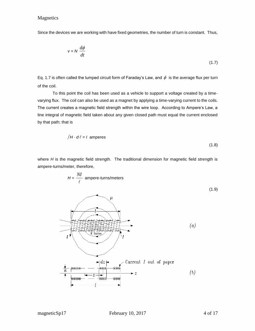
The current creates a magnetic field strength within the wire loop. According to Ampere’s Law, a

line integral of magnetic field taken about any given closed path must equal the current enclosed

by that path; that is

H d = I amperes

(1.8)

where H is the magnetic field strength. The traditional dimension for magnetic field strength is

ampere-turns/meter, therefore,

H =

NI ampere-turns/meters

(1.9)

Magnetics


Figure 2: (a) A solenoid of N turns with current I flowing; (b) a cross-section of the solenoid.

The total current into or out of the page is NI, and the amount in section dz is NI(dz/ ).

Magnetic field strength is related to magnetic flux density by the magnetic permeability of

the medium. For an air-cored solenoid as shown in Figure 2,

B = Ho

webers/meter2

(1.10)

After substituting in Eq. 1.9, the flux density becomes

B =

NIo

Tesla

(1.11)

Eq. 1.11 is a valid engineering expression for coils where > > a. The more exact expression is

B = 2/122

)4( a

NIo

Tesla

(1.12)

For a > > ,

B = a

NIo

2

Tesla

(1.13)

is sufficiently accurate. Figure 2 shows all geometries and defines all the variables.

It is obvious from Eqs. 1.9-1.13 that the magnetic field strength generated in the coil is

directly proportional to the current applied. If two excited coils are placed near each other, they will

be attracted toward or repulsed from each other with a force described by the following:

Magnetics


F = d

o

B2

2

Newtons

(1.14)

Where B is the mutual flux density linking the two coils and d is the distance between the two coils.

Obviously, the force can be either attractive or repulsive depending upon the field polarities, and

the force can be controlled by varying currents applied to the coils.

In all cases of DC excitation there is no generated emf after the initial transient dies out.

The transient is caused by the inductance of the coil that is defined as

L = i

Henrys

(1.15)

Geometrically, the inductance is

L = R

N2

=

AN 2

Henrys

(1.16)

Where N is number of turns, A is area of the flux path, is length of the flux path, and in the

permeability of the flux path. Obviously, the inductance of a device is determined by geometry

(N,A, ) and material characteristics ( ).

From Eq. 1.15, we find that

= Li Weber – turns

(1.17)

From Eq. 1.6, with Eq. 1.17, the terminal voltage required to force a current through an inductance

is

v = dt

d = L

dt

di+ 1

dt

dL

(1.18)

Magnetics


if the coil is ideal or of a super-conducting material. Real coils, such as those in the laboratory,

have resistance that also must be overcome when forcing current through the coil.

Therefore,

v = Ri + Ldt

di+ i

dt

dL

(1.19)

where R is the coil resistance.

The laboratory coils have a fixed number of turns that causes the third term on the right side of Eq.

1.l9 to go to zero. In addition, basic circuit theory tells us that the second term on the right side of

Eq. 1.19 goes to zero after the transient, 5-6 time constants. Therefore, for all practical purposes

the current through the coil with DC excitation is

I = R

V amps

(1.20)

regardless of the permeability of the magnetic path.

The permeability of the magnetic path is determined by the type of material in the path. If

the medium is air, or some other non-magnetic material, such as wood or glass, the permeability

is

= o

= 4 x 107 Henrys/meter

(1.21)

Permeability relates the flux density in the magnetic path to the magnetic field strength required to

achieve that density, thus

= H

B Henrys/meter

(1.22)

Obviously, if the medium is non-magnetic, the ratio described by Eq. 1.22 is constant.

Magnetics


Figure 3: Magnetization curve of commercial iron. Permeability is given by the ratio B/H.

If a ferromagnetic material, such as iron, is placed in the flux path, we find that much more

flux is produced for a given current. Figure 3 shows a typical magnetization curve for commercial

iron. On the curve

H

B = =

r

o Henrys/meter

(1.23)

where r is the relative permeability of the material. Figure 1.3 shows a peak relative permeability

exceeding 6000, which means for a given current, the iron core will have 6000 times the flux density

of an air core. A referral to Eq. 1.16 shows that the inductance of the coil will be 6000 times greater

if the applied current causes the system to operate at the point of maximum relative permeability.

For DC excitation, where the current is constant, the inductance is controlled by varying the cross

sectional area of the iron which causes the flux density to vary.

When AC excitation is applied to the coil, the results are different. The third term on the

right side of Eq. 1.19 can still be set to zero, but the second term on the right side cannot be zero

Magnetics


because the current is now a time-varying quantity. The second difference from the DC case is the

addition of a time-varying flux and a non-zero terminal voltage, as described by Eq. 1.7, appearing

across the coil. If we assume that the coil has an air core and that, for the time being, the resistance

is negligible, then the total applied voltage appears across the coil and causes flux to be produced.

The flux must be such that its time derivative multiplied by the number of linked turns exactly

matches the applied voltage. If we further assume that the applied voltage is sinusoidal, then the

flux must vary as a cosine such that

N

1 )()( tdttv Webers

(1.24)

Magnetic flux is actually produced by current (Eq. 1.8), so Eq. 1.24 must imply that the power

supply which is producing the sinusoidal voltage must also supply a co-sinusoidal current. This

current must have sufficient magnitude to produce the required flux.

The flux and current are related by the permeability of the magnetic path, which in turn is

a function of the material used for the magnetic path. If the path consists of ferromagnetic material,

it takes much less current to produce the required flux. In fact, if the voltage applied to the coil is

held at a constant RMS value, the required flux also has a constant RMS magnitude. The current

required to produce this constant flux varies inversely with the relative permeability of the magnetic

path.

Magnetics


Figure 4: Hysteresis loops of soft magnetic materials, which are easy to magnetize and demagnetize, and those of hard magnetic materials. The former is useful in transformers and machinery, whereas the later finds application in permanent magnets. The flux and current relationship is made more complex by the non-linear characteristics

of ferromagnetic materials, as shown in Figure 3. In addition, ferromagnetic materials exhibit

hysteresis characteristics shown in Figure 4. Since, in most cases of AC excitation and particularly

in a teaching laboratory, the strength of the AC source far exceeds that of the load, the source

voltage tends to maintain its sinusoidal wave shape. As discussed above, the flux must maintain

its sinusoidal nature. There, any non-linearities due to the flux path will appear in the current wave

shape. Figure 5 shows the result of a contained flux wave on a non-linear iron flux path. The

current shows a definite third harmonic flux wave on a non-linear iron flux path. The current shows

a definite third harmonic component. Note that the third harmonic is caused by a stiff sinusoidal

voltage source which causes an essentially sinusoidal flux within a non-linear magnetic path.

Magnetics


Figure 5: (1) Upper half of energy loop. (b) Sinusoidal flux and exciting current waves. (c) Waves of induced voltage, flux, and exciting current.

Figure 6: Two circuits with mutual inductance.

Magnetics


Figure 6 shows two coils sharing a common flux; called mutual coupling. If circuit 1 of the

figure is excited by an AC source, then the flux linking circuit 2 is time varying. The flux linking

circuit 2 causes a voltage to appear across the terminals of circuit 2 (Faraday’s Law). Thus, we are

seeing an indication of magnetic flux in circuit 2 due to the excitation current in circuit 1. This is the

concept of mutual inductance, which, in this case, is the inductance from circuit 1 to circuit 2, thus,

ANN

iL

21

1

2

12 Henry

(1.25)

where N1 and N 2

are the effective number of linked turns on each coil, A is the area of the

magnetic path, and is the length of the magnetic path. It is seen from Figure 6 that the effective

number of linked turns can be changed by varying the mutual geometry of the coils. Eq. 1.25 notes

the effects of coil geometry and permeability.

SUGGESTED PROCEDURE

1. Connect experimental set-up shown in Figure 7. Low voltage coils are found in the

laboratory shelf for each bench; they’re the coils with visible windings (use the large wire

coil). The permanent magnets and integrators are in the drawer on the lower side of the

bench. Set the oscilloscope using the procedure below. Then move the magnet in and out

of the coil at two speeds and different polarities. Record, andamplitude Record

waveform v, and Φ

Steps for configuring the oscilloscope

Select Default Setup

Select CH_1 Menu

Coupling = DC, BW Limit = Off, Volts/Dev = Coarse

Probe: > Voltage >Attenuation = 1X > Back

Invert = Off

Adjust the Volts/Div knob to 100 mV / Div

Select CH_2 Menu

Coupling = DC, BW Limit = Off, Volts/Dev = Coarse

Probe: > Voltage >Attenuation = 1X > Back

Invert = Off

Adjust the Volts/Div knob to 50 mV / Div Set the Horizontal

Magnetics


Sec/Div = 100mS Select Trig Menu

Type=Edge, Source=CH_1, Slope=Rising, Mode=Normal, Coupling=DC

Adjust Trigger Level knob: Level= between 20mv and 100mv

Select Single Seq

Press Ch_1 in the vertical menu buttons

Press Measure, and Select Measurement for Ch_ 1 top buttom. Press type until, Pk-Pk, then

Back.

Press Ch_2 in the vertical menu buttons and select Pk-Pk again Press Measure, and Select

Measurement for Ch_ 2 second buttom. Press type until, Pk-Pk, then Back.

Record the voltage and flux waveforms and record |𝑣| and |𝜙|.

2. Using the coil with the largest wire, connect the circuit shown in Figure 8. There are two

DC power supplies on the console. They are all the same, so use the most convenient.

To set the DC power supply follow the following procedure:

Be sure all knobs are turned fully counter-clockwise for voltage and at the 9:00 position for

current. Turn on DC supply. Increase voltage level slightly until DC ammeter gives a read-

out. Adjust current knob until 3.5 Amps (safety current limit) register on the Ammeter set

the Ammeter to DC current. Decrease voltage level to zero and remove short-circuit

across the coil.

Increase the voltage level. Using the voltage control set current to 3 amperes, energize the

coil and observe the force on the permanent magnet. Reduce current to 2 and 1 Amps

magnitudes and different magnet ends. Use the right hand rule to fine the magnetic

polarities of the field in the coil. Observe the forces of attraction and repulsion so that you

can determine the magnet’s polarities. As you run these experiments, keep the general

concepts of electromagnetic forces and energy conversion in mind.

3. The circuit show in Figure 9 is used for experiments required AC excitation. All equipment

taken from the shelves must be replaced on the shelves at the completion of the laboratory

period. The voltage across the 1 (found on the equipment shelf) is directly proportional

to the current through the resistor.

Now place the two coils directly next to each other in the position of maximum coupling.

This position creates maximum coupling because the flux that passes through any given

surface area of one coil passes through any cross-sectional area of the other coil. Adjust

Magnetics


the Single-Phase AC Source so the RMS current is 3 amps, make sure the Ammeter is set

to AC current. Note the RMS voltage across the excited coil (primary Heavy wire)

because during the next procedures this voltage should be kept constant. Insert three iron

strips at a time, through the windows of both coils and record RMS values for voltage,

current, and flux while maintaining constant voltage. Also, record the voltage and flux

wavesforms as the number of iron strips is varied.

No. strips Voltage RMS Current RMS Flux

0

3

6

9

Switch the oscilloscope to X-Y mode. To do this press the DISPLAY button and select

Format from the horizontal menu and XY from the vertical menu. The versus I curve is

displayed on the screen. Record the waveform of the versus I curve for air and various

numbers of steel strips while keeping the voltage constant.

If the hysteresis curve contains some unexpected loops, adjust the 100Ω potentiometer,

this should permit filtering them out. Record the waveforms and observe the changes in

the hysteresis loop using 3 iron strips when varying the terminal voltage for three different

values.

Record the hysteresis waveforms when biasing the 3 iron strips at one end with a

permanent magnet.

Using only 3 iron strips verify that the permeability of saturated iron is the same

as the permeability of air (observe the 3 amp current limit).

Magnetics


REPORT follow the template

1. Explain the observations made in Part 1 in terms of Faraday’s Law. Note particularly the

factors affecting the polarity, magnitude, and shape of the voltage and the relationship

between voltage and flux.

2. Explain the results of Part 2 in terms of magnetic polarities, current magnitudes, and the

general concepts of electromagnetic forces.

3. Explain the observations of Part 3 in terms of mutual coupling and permeability. Why is

the terminal voltage across the coil held constant? What happened to the current as iron

was added or subtracted? What happened to the fluxes? Describe the final observation

in terms of Figure 3. If you are designing an electromechanical device that requires linear

operation, what parameters need to be considered? How can you modify your design to

minimize eddy currents, and in return, how does this modification affect your device?

4. Using your knowledge of electromechanical devices and the results of this experiment,

what are some physical entities that affect saturation? Also, what design parameters can

be altered to prevent saturation?

Magnetics


Figure 7

Figure 8

Magnetics


AC

A

V

Diff amp scope CH1Diff amp Scope CH2

PosNegNegPos

1

10K

100 Black

White

H1

H4

X1

X3

Coil Heavy

wire

Coil Midsize

Wire

Passive

integrator

Figure 9

Documents

Magnetics - Virginia Tech · magneticSp17 February 10, 2017 1 of 17 EXPERIMENT Magnetics Faraday’s Law in Coils with Permanent Magnet, ... the magnetic flux through such a circuit