Maintaining Momentum Towards the MDGs: An Impact ... · An Impact Evaluation of Interventions to Improve ... Document of the World Bank ... to Meera Shekar of the World Bank’s nutrition

Maintaining Momentum Towards the MDGs: An Impact Evaluation of Interventions to Improve Maternal and Child Health and Nutrition Outcomes in Bangladesh

March 29, 2005 Operations Evaluation Department

Document of the World Bank

This document has a restricted distribution and may be used by recipients only in the performance of their official duties. Its contents may not otherwise be disclosed without World Bank authorization.

Abbreviations and Acronyms

ANC Ante-Natal Care BCG Bacillus Calmette-Guerin BDHS Bangladesh Health Survey BFS Bangladesh Family Survey BINP Bangladesh Integrated Nutrition

Project BMI Body-Mass Index BRAC Bangladesh Rural Advancement

Committee BRSFM Bangladesh Retrospective Survey

of Fertility and Mortality CAS Country Assistance Strategy CBNC Community-Based Nutrition

Component CNP Community Nutrition Promoter CPS Contraceptive Prevalence Survey DFID Department for International

Development (UK) DHS Demographic and Health Surveys DPT Diphtheria, Pertussis and Tetanus EOC Emergency Obstetric Care EPI Expanded Program of

Immunization FHV Family Health Visitor FSSAP Female Secondary School Stipend

Program FWA Family Welfare Assistant FWC Family Welfare Center GoB Government of Bangladesh HA Health Assistant HAZ Height-for-Age Z score HKI Helen Keller International HPSP Health and Population Sector

Project HPNSP Health, Population and Nutrition

Sector Project IEC Information, Education and

Communication I-PRSP Interim Poverty Reduction

Strategy Paper

IUD Intra-uterine device JFS Joint Finance Scheme KP Knowledge and Practice MCH Maternal and Child Health MDGs Millennium Development Goals MOFHW Ministry of Family, Health and

Welfare NGO Non Government Organization NIDS National Immunization Days NNP National Nutrition Program NORAD Norwegian Agency for

Development NSP Nutritional Surveillance Project OED Operations Evaluation

Department PCR Project Completion Report PHP Population and Health Project PPS-BD Participatory Practitioner’s

Society-Bangladesh READ Research Evaluation Associates

for Development SIDA Swedish International

Development Agency TBA Traditional Birth Attendants TFR Total Fertility Rate TMSS Thengamara Mohila Sabuj Sangha TTBA Trained Traditional Birth

Attendant UHZ Upazilla Health Complex UNFPA United Nations Population Fund UNICEF United Nations Children’s

Emergency Fund USAID United States Agency for

International Development SAR Staff Appraisal Report WAZ Weight-for-Age Z score WDI World Development Indicator WHO World Health Organization WHZ Weight-for-Height Z score

Director-General, Operations Evaluation : Mr. Gregory K. Ingram Director, Operations Evaluation Department : Mr. Ajay Chhibber Manager, Sector, Thematic, and Global Evaluation Group : Mr. Alain Barbu Task Manager : Mr.. Howard N. White

i

Table of Contents

Acknowledgments ..............................................................................................................v

Executive Summary........................................................................................................ vii

1. Maternal and Child Health in Bangladesh: A Record of Success ...........................1

Scope of the Study ....................................................................................................4

2. Health, Family Planning and Nutrition Services in Bangladesh: An Overview ....8

Family Planning Programs......................................................................................8

Health Services ......................................................................................................11

Nutrition.................................................................................................................14

3. Trends in Under-Five Mortality, Nutrition and Fertility.......................................16

Patterns of Mortality Decline ................................................................................16

Anthropometric Outcomes .....................................................................................17

What Has Been Happening to Fertility?................................................................18

4. Impact of Specific Interventions on Child Health and Fertility ................................21

Income Growth Accounts for Some, But Not All, Improvement in Outcomes .......21

Under-five Mortality ..............................................................................................24

Fertility Reduction .................................................................................................33

Nutrition.................................................................................................................35

5. A Closer Look at Nutrition: The Bangladesh Integrated Nutrition Project ........36

Overview of the Project .........................................................................................37

Project Coverage and Targeting ...........................................................................38

Acquiring Knowledge.............................................................................................41

Turning Knowledge into Practice: the Knowledge Practice Gap .........................42

The Nutritional Impact of BINP Interventions.......................................................45

Testing the Theory in Practice - How Well Did the Causal Chain Operate?........48

6. Lessons Learned.........................................................................................................50

ii

Annexes

Annex A. Trends in Maternal and Child Health Outcomes..............................................55

Annex B. Cross-Country Analysis of Child Health and Nutrition Outcomes ...................58

Annex C. Neonatal, Postnatal, and Child Mortality in the 1990s......................................76

Annex D. Child Malnutrition During the 1990s ..............................................................134

Annex E. Women’s Agency, Household Structure, and Health Outcomes.....................154

Annex F. Fertility.............................................................................................................172

Annex G. Analysis of BINP’s Community-Based Nutrition Component .......................191

Annex H. DFID and World Bank Programs in Bangladesh ............................................236

Annex I. Agricultural Production, Natural Disasters, Seasonality and Nutritional Outcomes....................................................................................................................................242

Annex J. Approach paper.................................................................................................249

References....................................................................................................................259 Boxes

Box 1.1 Measures of welfare outcomes.................................................................................... 2 Box 4.1 Which Children Get Immunized? ............................................................................. 26 Box 4.2 Polio Eradication in Bangladesh ............................................................................... 27 Box 5.1 Qualitative Perspectives of the Knowledge - Practice Gap: the PPS-BD study ....... 44 Figures

Figure 1.1 Both Under-five Mortality and Fertility Have Fallen Rapidly................................ 3 Figure 2.1 Immunization coverage of children aged 12-23 months …………………..…… 13 Figure 3.1 Nutritional Status Improved in the 1990s (proportion <-2SDs WAZ and HAZ).. 17 Figure 3.2 Data From Different Sources Present a Consistent Picture (WAZ) ...................... 18 Figure 3.3 Fertility decline continued in the 1990s according to a range of indirect measures

......................................................................................................................................... 20 Figure 3.4 Knowledge of modern contraceptives is universal and use continues to rise ....... 20 Figure 4.1 Bangladesh’s improvement in social outcomes is greater than can be explained by

economic growth alone ................................................................................................... 22

iii

Figure 5.1 Various Factors Affect Women’s Participation, but Restrictions on Women’s Mobility in More Conservative Areas are the Most Important....................................... 38

Figure 5.2 Women Living in Project Areas are More Likely to Have Nutritional Information, Especially if They Participate in Project Activities ........................................................ 42

Figure 5.3 The Knowledge-Practice gap in project areas: more women say they know good behavior than actually practice it .................................................................................... 43

Figure 5.4 Rice Production and Daily Energy Supply Have Grown Rapidly in the Late 1990s......................................................................................................................................... 47

Tables

Table 3.1 Fertility Decline Has Always Been Erratic Based on Direct Estimates, but Continues into The 1990s Using Indirect Ones .............................................................. 19

Table 4.1 Growth in GNP Per Capita Accounts for at Most One-Third of The Reduction in Mortality… and Less Than a Fifth of Lower Fertility.................................................... 22

Table 4.2 Significant Determinants of Infant and Child Mortality......................................... 25 Table 5.1 Many Factors Prevent Women from Putting Nutritional Advice into Practice,

Though the Project Partially Overcomes Some of These ............................................... 44 Table 5.2 Cost of Nutrition Improvements and Mortality Reduction (US$).......................... 46 Table 5.3 Links in the Causal Chain....................................................................................... 49

v

Acknowledgments

This study is the second in a series of three impact studies being conducted by OED under a DFID-OED partnership agreement.1 In these studies OED is exploring different ways of carrying out ex post impact analysis in cases for which no impact evaluation framework was put in place at the start of the intervention. For the first study, of Ghana basic education (World Bank, 2004), a survey was commissioned to follow on from a nationally representative household and school survey conducted fifteen years earlier. This second study is based on existing data sets: the Bangladesh Demographic and Health Surveys, the Household Income and Expenditure Survey, two data sets related to the Bangladesh Integrated Nutrition Project - the evaluation data set and that collected by Save the Children - and data from Helen Keller International’s Nutritional Surveillance Project. Thanks are due to Meera Shekar of the World Bank’s nutrition hub, Dora Panagides of HKI and Anna Taylor and Arabella Duffield of Save the Children for facilitating access to the latter three data sets. This report was prepared by Howard White, with assistance from Nina Blöndal, Edoardo Masset and Hugh Waddington, and inputs provided by Professor Kabir and Dr. Sayed Haider of Research Evaluation Associates for Development (READ) and Dr. Sharifa Begum of the Bangladesh Institute of Development Studies (BIDS). In addition, a background paper was commissioned from the Participatory Practitioner’s Society-Bangladesh (PPS-BD). Preparation of the report was assisted by Alain Barbu, Martha Ainsworth and Denise Vaillancourt. Professor Nicholas Mascie-Taylor (University of Cambridge) and Dr. Arabella Duffield (Save the Children UK) acted as external reviewers. Comments were also received by Harold Alderman, Farial Mahmud, Md. Abdul Maleque (of the Implementation, Monitoring and Evaluation Department of the Ministry of Planning in Bangladesh), Bina Valaydon, the Planning Commission of the Government of Bangladesh, and Bernabé Sánchez, Nick York and Shona Wynd of DFID Evaluation Department. Thanks are due to all those in the Government of Bangladesh, NGOs and donor agencies who provided their time and support to the undertaking of this study. In the World Bank office in Dhaka, Rafael Cortez, Farzana Ishrat and Shirin Jahangeer provided valuable inputs, and excellent logistical support was provided by the support staff of the Health Project Support Office, including arranging a presentation of preliminary findings. From DFID, Dinesh Nair and Neil Squires provided useful guidance. Thanks are due to Kaosar Afsana of BRAC and Mohammed Azizul Hoque of Thengamara Mohila Sabuj Sangha for their assistance in trips to the field. Administrative support was provided by Soon Woon-Pak. The report was edited by Bill Hurlbut.

1 Financial support was also provided through Danish Consultant Trust Funds.

vii

Executive Summary

1. Improving maternal and child health and nutrition is central to development goals. The importance of these objectives is reflected by their inclusion in poverty-reduction targets, such as the Millennium Development Goals (MDGs) and Bangladesh’s Interim Poverty Reduction Strategy Paper, supported by major development partners including the World Bank and DFID. This report addresses the issue of what publicly-supported programs and external assistance from the Bank and other agencies can do to accelerate attainment of targets such as reducing infant mortality by two-thirds. The evidence presented here relates to Bangladesh, a country which has made spectacular progress but needs to maintain momentum in order to achieve its own poverty reduction goals.

2. The report addresses the following issues: (1) What has happened to child health and nutrition outcomes and fertility in Bangladesh since 1990? Are the poor sharing in the progress which is being made? (2) What have been the main determinants of MCH outcomes in Bangladesh over this period? (3) Given these determinants, what can be said about the impact of publicly and externally-supported programs – notably those of the World Bank and DFID - to improve health and nutrition? (4) To the extent that interventions have brought about positive impacts, have they done so in a cost effective manner?

Trends in Under-Five Mortality, Fertility and Nutrition

3. Despite an inauspicious start coming out of war and famine, Bangladesh has achieved spectacular rates of progress in the last two decades, most notably with respect to fertility decline. Contrary to common perceptions, fertility continued to decline during the 1990s. Under-five mortality has also been reduced at a substantial rate, Bangladesh being one of the few countries to achieve a sufficient rate of reduction to achieve the MDG of a two-thirds decline by 2015. The exception to these successes has been nutrition. Physical measures of nutritional status only began to show some improvement in the 1990s, and malnutrition remains at high levels.

4. Improvements in these outcomes have been spread across all Bangladeshis. Although children of the poor are more likely to suffer premature death, this gap is narrowing, with mortality rates falling faster among the poor than the non-poor. Contraceptive use and low fertility are also common among the poor.

Sources of Under-five Mortality Decline

5. Analysis of the determinants of mortality using both cross-country and Demographic and Health Survey (DHS) data shows that a variety of factors have been behind the falling number of deaths. Improved economic well-being is the most important reason for lower child mortality, but plays less of a role for infants. Social sector interventions – both health and education – are also found to matter, with expanded immunization coverage and greater female enrolment in primary and secondary education both playing a substantial part in mortality reduction. The results also show a pronounced sex bias in mortality against girls, especially in the Sylhet and Chittagong divisions. Analysis of selected interventions reveals the following:

viii

• Immunization coverage was at less than 2 percent in the early 1980s, but grew in the latter part of the decade (largely with the support of UNICEF, but later also other donors including the World Bank) so that by 1990 close to half of all children were fully vaccinated in their first 12 months. Immunization has averted over 2 million child deaths in the last two decades, at a cost of between $100 and $300 per life saved.

• The World Bank financed the training of approximately 14,000 traditional birth attendants (TBAs) until the late nineties, at which point training TBAs was abandoned following a shift in international opinion toward a policy of all births being attended by Skilled Birth Attendants. However, the evidence presented in this report shows that training TBAs saved infant lives, at a cost of $220-800 per death averted.

• Female secondary schooling expanded rapidly in the 1990s, especially in rural areas partly as a result of the stipend paid to all female students in grades 6-10 in rural areas supported by Norwegian aid, the Asian Development Bank, the World Bank and government. Amongst the benefits of the increase in female secondary schooling are lower mortality, at a cost of $1,080-US$5,400 per death averted.

• Rural electrification, supported through three World Bank programs in the 1980s and 1990s, reduces mortality through income effects, improving health services, making water sterilization easier and improving access to health information, especially from TV. Taking these various channels into account means that children in households receiving electrification have an under-five mortality rate 25 per 1,000 lower than that of children in non-electrified households. Based on historic costs, this amounts to $20,000 per life saved, and $40,000 based on current connection costs.

Nutrition

6. In order to address the poor state of nutrition, the government implemented, with World Bank assistance, the pilot Bangladesh Integrated Nutrition Project (BINP). The core of BINP is the Community-Based Nutrition Component (CNBC), which promotes nutritional counseling to bring about behavior change, complemented by supplementary feeding for pregnant women and young children.

7. Analysis of the causal chain from BINP inputs to child anthropometric outcomes shows the following: (1) there is a weak link in the chain as behavioral change communication has been excessively focused on mothers, who are often not the main decision maker for all nutrition-related practices; (2) program coverage is generally high in project areas, but notably lower in more conservative thanas (sub-districts), especially among women who live with their mothers-in-law; (3) there are some deficiencies in targeting: (a) too strict a criterion was applied in admitting malnourished children to supplementary feeding, while admitting children who were growth faltering but probably well-nourished, (b) feeding of pregnant women excluded many who were eligible while including a proportion who were not; (4) a large proportion of mothers of children receiving supplementary feeding claimed to have not received nutritional counseling; (5) there is a substantial knowledge-practice gap, whereby women do not turn the advice they receive into practice: economic resource and time constraints are a major reason for this; and (6) the impact on pregnancy

ix

weight gain is too small to have a substantial impact on birth weight, which is a common result from similar programs in other countries; mother’s pre-pregnancy nutritional status is a more important factor in low birth weight than pregnancy weight gain and might therefore have been a better focus for the project.

8. The list in the previous paragraph may be read as a list of problems to be fixed in the project, as to some extent they have been under the expanded National Nutrition Project – the targeting criteria for children’s supplementary feeding have been revised and another attempt made to reach men with nutritional counseling. But the program has not been a very cost effective means of improving nutritional status – which has improved generally with the acceleration in food availability associated with the yield-driven increase in rice production since the late nineties, and consequent reduction in the real price of rice. Simulations show that simply giving food to families with children would have had a larger nutritional impact. The cost per life saved from the hypothetical rice ration is just over $2,000, half the cost of lives saved by BINP.

Fertility Reduction

9. The rate of fertility reduction in Bangladesh is shown to exceed that which may be expected from other socio-economic developments, such as income growth and expanding female education. While socio-economic developments, including the demographic transition, explain a part of Bangladesh’s rapid fall in fertility, a large part is attributable to the country’s family planning service, built up with substantial external support in the years following liberation in 1971. The continued decline of fertility in the 1990s, driven by rising contraceptive prevalence, demonstrates the continued effectiveness of this program.

10. The government’s HNP Strategic Investment Plan highlights the role of increasing the age at marriage as a means of reducing fertility, and several programs, including the counseling provided under BINP, promote getting married later. It is a condition of the female secondary school stipend program, supported by the Bank amongst others, that recipients remain unmarried. It is true that the age at marriage in Bangladesh is low, with half of all women marrying by age 14. It is also true that there is a well-established international pattern whereby increasing the age at marriage drives down fertility. But this pattern should not be expected to be observed in Bangladesh for two reasons: (1) raising the age at marriage of girls aged 13 or less has no effect on the age at which they have their first child (so as the age at marriage has risen the gap from marriage to first birth has fallen), and (2) if a woman plans to have only 3-4 children, as the majority of Bangladeshi women do, then this can be accomplished whether child bearing begins at 15 or 20. The direct effect of expanding secondary education will be muted, as Bangladesh has already attained fertility levels comparable to those in countries with higher education levels. Hence raising the age at marriage, while desirable for both maternal and child health (children born to young mothers have a greater chance of premature death), will have little impact on the number of children borne by each women during her reproductive years - though there would be a temporary tempo effect on the total fertility rate, and there will be a second-order effect as the mortality reducing effect of later births will reduce the desired number of births. Instead high fertility households should be targeted, partly by an attempt to restore the use of permanent contraceptive measures to their previous levels. Efforts should also be made to tackle son

x

preference which creates a barrier to fertility decline. And continued success in reducing mortality will also help reduce fertility.

Lessons Learned

11. The following general lessons follow from the analysis in this report:

• Externally supported interventions have had a notable impact on MCH-related outcomes in Bangladesh. Immunization has proved particularly cost effective, and has saved the lives of up to two million children under the age of five

• World Bank support to sectors outside of health has contributed to better child health outcomes

• Small amounts of money save lives…though the amount varies significantly by intervention

• Although interventions from many sectors affect maternal and child health outcomes, this fact need not imply that multi-sectoral interventions are always needed

• World Bank support for training traditional birth attendants has reduced neonatal mortality…but this program has now been abandoned following the international trend toward support for skilled birth attendants

• Programs should be based on local evidence, rather than general conventional wisdom

• Gender issues are central to health strategies in Bangladesh. More attention is needed to redressing gender biases to maintain momentum in mortality decline and fertility reduction. But traditional attitudes are not the absolute constraint on service provision which is sometimes suggested.

• The Bank’s BINP has improved nutritional status, but not by much less than planned. Serious attention needs to be given to ways of improving both the efficacy and efficiency of the program - or if not possible then to consider alternatives to scaling up.

• Rigorous impact evaluation can show which government programs and external support are contributing most to meeting poverty reduction goals

• National surveys can be used for evaluation purposes, but some adaptations would make them more powerful, notably a more detailed community questionnaire

1

1. Maternal and Child Health in Bangladesh: A Record of Success

Improving maternal and child health is central to the development challenge. Bangladesh has a remarkable record in the reduction of under-five mortality and fertility, but less impressive achievements with respect to nutrition. This study examines the impact of inventions from various sectors – health, population, nutrition, education and electrification – on these outcomes. Will existing interventions be adequate to maintain momentum toward the achievement of poverty reduction goals, or are changes required?

1.1 Improving maternal and child health (MCH) and nutrition is central to the development challenge. This is reflected in the incorporation of MCH outcomes in development goals. Two of the eight Millennium Development Goals (MDGs) refer to MCH outcomes -- reducing under-five and maternal mortality -- and child malnutrition is an indicator for the first MDG goal. Four of the ten goals in Bangladesh’s Interim Poverty Reduction Strategy Paper relate to MCH. These four are to (1) reduce infant and under-five mortality rates by 65 percent, and eliminate gender disparity in child mortality; (2) reduce the proportion of malnourished children under-five by 50 percent and eliminate gender disparity in child malnutrition; (3) reduce the maternal mortality rate by 75 percent; and (4) ensure reproductive health services for all.2 These goals are reflected in the Bank’s Country Assistance Strategy (CAS): human development is listed as the first ‘development priority’, and the second of the four ‘thrusts’ in the CAS is to “consolidate gains in human development, addressing development challenges in education, health, and nutrition”.3

1.2 Adoption of a results-based approach requires understanding the main drivers behind changes in target outcomes. Which publicly-supported interventions can accelerate the pace of improvement and so secure the achievement of development goals? Have the interventions supported by the Bank and DFID contributed to meeting the goals they set themselves in their respective country strategies? This report addresses these questions in the context of Bangladesh, a country which has made notable progress but needs to maintain momentum in order to achieve its own poverty reduction goals. The following outcomes are analyzed: infant and child mortality, child nutrition, nutritional status of pregnant women and low-birth weight, and fertility (see Box 1.1). Maternal mortality is excluded on account of lack of data.4 However, fertility is included as a known correlate of maternal mortality, as well as being related to child health and nutrition.

1.3 The years immediately following Bangladesh’s liberation in 1971 were inauspicious ones for the prospects of development. Emerging from a violent struggle which cost over one million lives, the country was beset by a famine responsible for 2. Ministry of Finance Bangladesh: A National Strategy for Economic Growth, Poverty Reduction and Social Development, March 2003: pp. 7-8.

3. Country Assistance Strategy for Bangladesh, World Bank, February 2002, Report No. 21326-BD.

4. Data from the 2003 Maternal Mortality Survey were not available for analysis.

2

at least another quarter of a million deaths. Nearly one in four children were dying before reaching their fifth birthday, reflecting the highest under-five mortality rate in the region, and one of the highest in the world.5

1.4 But by the start of the 1980s the situation had changed. The decline in infant and child mortality which began slowly in the 1960s accelerated (Figure 1.1).6 By 2000 under-five mortality had fallen to 82 per 1,000 live births. This rate is now

5. The under-five mortality rate in 1970 was 239 per 1,000 live births, compared to 202 for India, 181 for Pakistan (excluding Bangladesh) and just 100 for Sri Lanka.

6. Social indicators are often built upon fairly shaky statistical foundations. However, as shown in Annex A, Bangladesh has benefited from various surveys so that the data are unusually reliable. The exception has been maternal mortality, but a new maternal mortality survey has changed the situation also in this regard.

Box 1.1 Measures of welfare outcomes

Mortality

The three mortality measures are:

• Infant mortality rate (IMR), the probability of death before an infant’s first birthday, usually expressed per 1,000 live births

• Child mortality rate (CMR), the probability of death between a child’s first and fifth birthdays, expressed per 1,000

• Under-five mortality rate (U5M), the probability of death before a child’s fifth birthday.

Anthropometric measures

The nutritional status of children under-five is often monitored through measurements of their height, weight and age. These three pieces of information are used to calculate three ratios:

• Height for age (stunting): a measure of long-run nutritional status • Weight for height (wasting): a measure of short-run nutritional status • Weight for age (underweight): a combination of the above two measures

Nutritional status is determined by converting a measure to a z score, i.e. subtracting the mean and dividing by the standard deviation (SD) from a reference population. The corresponding statistics are called the height for age z score (HAZ), weight for height z score (WHZ) and weight for age z score (WAZ). Values of less than -2 (i.e., 2 SDs below the reference mean) are taken to indicate malnutrition and less than -3 severe malnutrition.

For adults, the appropriate measure is the Body Mass Index (BMI), which is equal to a person’s weight in kilograms divided by the square of their height in meters. A BMI of less than 18.5 indicates that a person is underweight.

Fertility

The most common measure, the total fertility rate (TFR), is the number of children a woman would have if her child-bearing equaled the age-specific fertility rates of women currently in those age groups. That is, TFR is a cohort measure. In the presence of declining fertility, a woman entering her child-bearing years is expected to have fewer children than the TFR, whereas the average number of children born to women who have completed their reproductive years will exceed the TFR.

3

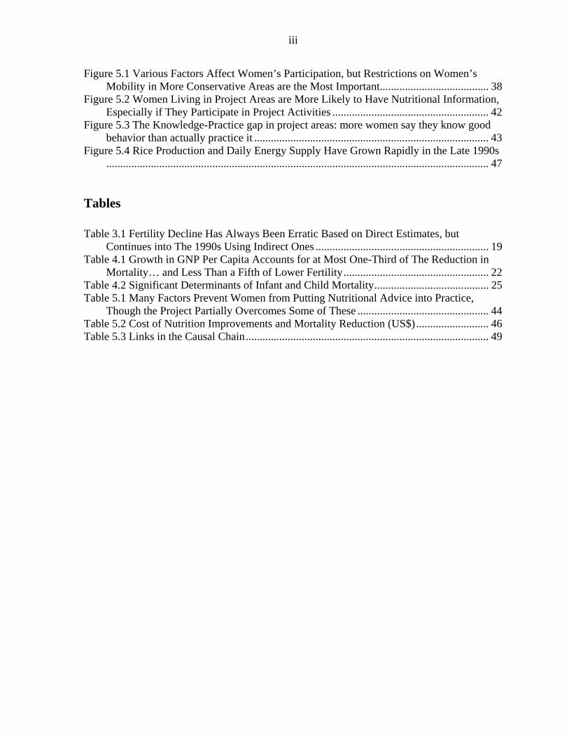
below that in neighboring countries and a sufficient rate of decline for Bangladesh to be one of the few countries on track to meet the Millennium Development Goal of a two-thirds reduction between 1990 and 2015. The country’s achievements with respect to fertility are even more remarkable. Fertility was very high, and possibly even rising, in the sixties and early-1970s, with each woman bearing an average of seven live births. A rapid decline in fertility starting in the mid-1970s has more than halved the total fertility rate.7 There was less progress regarding nutrition, with improvements in anthropometric indicators occurring only in the 1990s. Maternal mortality also remains very high.

Figure 1.1 Both Under-five Mortality and Fertility Have Fallen Rapidly

Source: Annex A 1.5 This report analyses the factors behind this success story, focusing on the 1990s. The main questions addressed are:

• What has happened to child health and nutrition indicators and fertility in Bangladesh since 1990? Are the poor sharing in the progress which is being made?

• What have been the main determinants of MCH and nutrition outcomes in Bangladesh over this period?

• Given these determinants, what can be said about the impact of publicly-supported programs to improve health and nutrition?

• To the extent that interventions have brought about positive impacts, have they done so in a cost effective manner?

7. Whether or not fertility decline continued into the 1990s is a matter of debate. This issue is explored in Chapter 3 and Annex F.

0

50

100

150

200

250

300

1960 1965 1970 1975 1980 1985 1990 1995 2000 2005

Und

er-fi

ve m

otal

ity

0.0

1.0

2.0

3.0

4.0

5.0

6.0

7.0

8.0

Tota

l fer

tility

rate

Under-five m ortality Total fertility rate

4

Scope of the Study

1.6 Maternal and child health and nutrition outcomes result from public policies and private actions in many sectors: not only health provision and choices, but also, for example, income-generation, education and infrastructure. This study focuses on a few selected interventions supported by the World Bank, DFID and other external agencies from both within and outside the population and health sector. The interventions have been selected on the grounds of (1) their demonstrated importance for health and nutrition outcomes, and (2) the involvement of external partners in supporting service provision.

1.7 Health, nutrition and population programs are clear candidates for inclusion in the evaluation on grounds of both an expected impact on MCH-related outcomes and and the level of externally-supported public provision of services. Bangladesh has benefited from a high degree of donor coordination in the health and population sector, under the auspices of five World Bank credits since 1975 with substantial levels of cofinancing from bilateral agencies, including the United Kingdom.8 The first three of these projects focused on establishing the country’s reproductive health system, but the fourth and fifth projects expanded coverage to all aspects of health care delivery. This study is mainly concerned with the period covered by the Fourth Population and Health Project (PHP IV, 1993-99) and the Health and Population Sector Project (HPSP, 1998-2004). HPSP marked the transition from coordinated project support to sector program financing (sector budget support); for example DFID health spending in this period was dominated by UK£25 million denoted as ‘World Bank time slice financing’.

1.8 Preparations are underway for the follow up Health, Population and Nutrition Sector Project (HPNSP), with further expansion in coverage. While nutrition activities were partly included in earlier health projects, a stand-alone pilot project, the Bangladesh Integrated Nutrition Project (BINP) was initiated in 1996. BINP, and the follow-on National Nutrition Project (NNP), embody a behavior change approach to improving nutritional status, an approach of growing importance in various areas of health care. This study re-examines the data from recent evaluations of BINP to determine the effectiveness of this approach.

1.9 Evidence of impact on MCH outcomes from two other sub-sectors is also assessed: female secondary schooling and rural electrification. Female education is a well-established correlate of child health and nutrition, a link confirmed by the empirical analysis in this study (Chapter 4 and Annexes C and D). The World Bank has been one of the agencies supporting the female secondary school stipend program (FSSAP), which is shown to have made a substantial contribution to the rapid growth in secondary enrolments. Electrification appears as a determinant of mortality in many studies, although the channels for this effect are not so well documented. Together with

8. For example, the United Kingdom financed fifteen separate activities under the Fourth Population and Health Project, totaling UK£ 15.5 million (close to US$30 million at current exchange rates). Close to half of this total was for ‘Support to NGO programs’, with substantial amounts also for strengthening nurse education (UK£ 2.8 million) and medical colleges (UK£3.1 million) (see Annex I).

5

other agencies, the World Bank supported rural electrification in Bangladesh through three projects in the eighties and nineties,9 so this link warrants further investigation.

1.10 It is worth mentioning some areas which have been excluded from the study, despite their importance to MCH outcomes: income-generating activities, disaster prevention and relief, and economic infrastructure. The many interventions whose main impact on health is via their income generation effects have been excluded from the analysis on two grounds. The first reason is that estimating income effects of interventions is a sizeable task in itself, and not one to which the data strategy adopted for this study was well-suited. The second reason is that while economic growth explains part of Bangladesh’s remarkable progress in improving social outcomes, it is not, as is shown in Chapter 4, the whole explanation.

1.11 A second sector excluded from this study is that of disaster prevention. Bangladesh is subject to repeated disasters, most notably flooding. A substantial amount of external support has gone to measures to prevent flooding and protect people from its consequences, as well as funds for relief and rehabilitation in the wake of such events.10 The success of these, and similar programs funded from other sources, is shown by the reduced death toll from natural disasters.11 These flood control measures should be important to preserving livelihoods (though some early Bank-supported projects had the opposite effect) and saving lives. But the number of deaths directly attributable to flooding, at less than 2,000 in each disaster year, is relatively small compared to the approximately 300,000 under-five deaths each year.12

1.12 Another area of great importance, but not considered in this study partly for the reason income-generating activities are excluded (difficulty in tracing the causal chain with the data to hand), is economic infrastructure. Large-scale infrastructure, such as the DFID-supported renovation of Chittagong port, have helped spur the rapid expansion of the garment industry, which has brought both economic growth and changes in the position of women. Other large projects, such as Jamuna bridge, have greatly reduced travel time across the country, promoting social and economic integration. Smaller scale rural roads, and particularly bridges, foster the integration of remote areas, facilitating access to markets and other services.13

9. Rural Electrification I: 1982-86; II: 1985-94; and III: 1990-99.

10. The World Bank has lent US$234 million for flood relief and drainage programs in the last two decades and DFID £59 million since 1991 (see Annex I).

11. The 1998 floods were far greater in terms of the affected area and infrastructure destroyed than those in 1988. But fewer than 1,000 people lost their lives in the 1998 floods compared to over 2,400 in 1988. And only 600 died in the 2004 floods which appear to be at least comparable to those in 1998.

12. Among older children drowning is now the major cause of death. But, as these figures show, these drownings are mainly accidents rather than the direct consequence of flooding. Figures on indirect deaths from flooding as a result of disease and malnutrition are less easy to come by, though there is such an effect (for some estimates see Del Ninno et al., 1991).

13. Moore (2003) argues that the remote nature of many communities, resulting in control of local politics by a small number of dominant families, in part results from difficulties in moving around the country. Infrastructure may thus be argued to have beneficial effects on political life, which in turn will improve service delivery.

6

Evaluation Approach

1.13 This study draws on the analysis of a number of existing data sets. Demographic and Health survey (DHS) data are used to model the determinants of child health and nutrition outcomes, and of fertility. Bangladesh has had three such surveys in the 1992, 1996 and 1999,14 allowing an analysis of the relative importance of the various determinants in explaining improved outcomes in the 1990s. This analysis informed the choice of sectors to be included in the evaluation.

1.14 The impact of different interventions is estimated through a structural modeling approach. That is, multivariate estimates are made of the outcomes of interest (mortality, nutrition and fertility), drawing on the state of the art in the literature. The endogeneity of behavioral factors, such as antenatal care and immunization, is controlled for through the use of appropriate instruments, and the selection bias from children who have died not being in the sample for the nutrition equation allowed for by a two part sample selection model. Further details on methodology can be found in the relevant Annexes (notably C, D and G) and in the Approach Paper (Annex J). Combining the marginal impact of different interventions on welfare outcomes with cost data allows cost effectiveness analysis to be carried out.

1.15 The analysis of nutrition is a partial exception to the above approach. The Bangladesh Integrated Nutrition Project (BINP) conducted a survey for evaluation purposes. This study presents a re-analysis of these data, modifying the control group using propensity score matching by drawing on the nationally representative Nutritional Surveillance Survey carried out by Helen Keller International. A theory-based approach is adopted, so that the causal chain by which inputs are intended to affect outcomes can be examined in detail

1.16 The main thrust of this approach is heavily quantitative. But any impact evaluation needs to place itself in context. Qualitative information is relevant to the analysis in various ways. First is the historical political context. Bangladesh has historically had a strong commitment to basic health, introducing an essential drugs policy in face of substantial opposition, but in recent years there is a poor record of delivering essential health at the field level (see Chapter 2). Second, is the changing role of women, and the way in which purdah may restrict their ability to access health services. A third important factor is the importance of the private sector, although this study focuses on services which have been provided by government with external support.

1.17 The findings from this study can be related to OED’s evaluation criteria of relevance, efficacy and efficiency. This chapter has already illustrated the relevance of interventions intended to improve maternal and child health and nutrition to Bangladesh’s poverty reduction goals. The efficacy of the interventions depends on establishing a link from supported activities to welfare outcomes, as is done in

14. The data from a fourth DHS survey, conducted in 2004, were not available for this study.

7

Chapters 4 and 5 of this report. Efficiency is determined using cost-effectiveness analysis, which is reported in the same chapters.

Overview of the Report

1.18 Chapter 2 presents background information on the evolution of health and family planning services in Bangladesh and the role of external agencies in supporting these programs. The record with respect to mortality, fertility and nutrition is presented in Chapter 3. The following two chapters examine the impact of selected interventions on health, nutrition and fertility outcomes. Chapter 6 concludes with lessons learned.

8

2. Health, Family Planning and Nutrition Services in Bangladesh: An Overview

Following independence Bangladesh established a substantial network of health and family planning facilities. This network, including staff costs, was largely financed by donor assistance during the first decade. Although facilities were created for both health and family planning, the focus of service delivery until the 1990s was on family planning, with the exception of immunization for which a successful campaign was launched in the mid-1980s. The family planning services were built up on a home visit system, similarly immunization operates through 8,000 outreach centers around the country. Plans to move to a fixed site system, for which construction of community clinics has been undertaken at donor expense, have met with very limited success. Expanding beyond its limited coverage in existing programs, a pilot Integrated Nutrition Project was launched in 1996, which is now being rolled out nation-wide.

Family Planning Programs

2.1 Family planning began with the voluntary Family Planning Association in what was then East Pakistan in 1952. A national family planning program was adopted in 1965, setting up a network of family planning clinics, run by the Family Planning Board. The program used incentives for both personnel and acceptors, promoting mainly sterilization and intra-uterine devices (IUDs). Success was limited, with fewer than 10 percent of couples having ever used contraception in 1969, though awareness of modern methods increased markedly. As a result of limited acceptance, fertility remained high, with a total fertility rate (TFR) of seven. Planned improvements in the program were interrupted by the liberation war in 1971. The newly independent government recognized population as one of the country’s most pressing problems: already by that time the country had the highest population density in the world.

2.2 The Government of Bangladesh’s efforts to reduce population growth cannot be separated from the role of external agencies, since these agencies were central from the outset, paying the majority of program costs, including salaries, in the early years. The country’s First Five Year Plan proposed a health and family planning system comprising a hospital in each district,15 which in some cases was supplemented by a Maternal and Child Welfare Center at sub-district level. Each thana was to have an Upazilla Health Complex (UHC), and then each union a Family Welfare Center (FWC). Each FWC is headed by a Medical Assistant, working with a Family Welfare Visitor (FWV) and a Pharmacist. The FWC’s staff comprise a female Family Welfare Assistant (FWA) and a male Health Assistant (HA). The FWV conducts satellite clinics, the FWA makes home visits and the HA has responsibility for malaria and epidemic control and environmental sanitation.

15. Bangladesh has six administrative divisions, further sub-divided into 64 districts. Each district has several thanas (formerly upazillas), of which there are 490 in total. Each thana (covering some 15-20 villages) is further sub-divided into several unions.

9

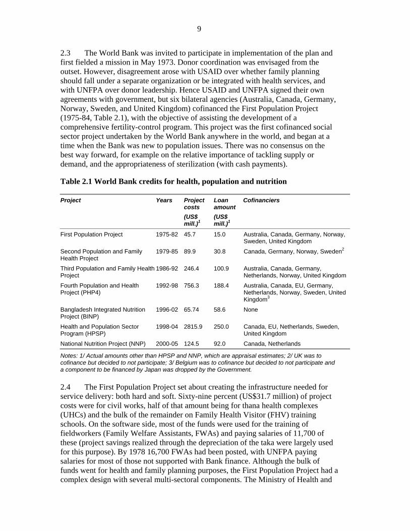
2.3 The World Bank was invited to participate in implementation of the plan and first fielded a mission in May 1973. Donor coordination was envisaged from the outset. However, disagreement arose with USAID over whether family planning should fall under a separate organization or be integrated with health services, and with UNFPA over donor leadership. Hence USAID and UNFPA signed their own agreements with government, but six bilateral agencies (Australia, Canada, Germany, Norway, Sweden, and United Kingdom) cofinanced the First Population Project (1975-84, Table 2.1), with the objective of assisting the development of a comprehensive fertility-control program. This project was the first cofinanced social sector project undertaken by the World Bank anywhere in the world, and began at a time when the Bank was new to population issues. There was no consensus on the best way forward, for example on the relative importance of tackling supply or demand, and the appropriateness of sterilization (with cash payments).

Table 2.1 World Bank credits for health, population and nutrition

Project Years Project costs

(US$ mill.)1

Loan amount (US$ mill.)1

Cofinanciers

First Population Project 1975-82 45.7 15.0 Australia, Canada, Germany, Norway, Sweden, United Kingdom

Second Population and Family Health Project

1979-85 89.9 30.8 Canada, Germany, Norway, Sweden2

Third Population and Family Health Project

1986-92 246.4 100.9 Australia, Canada, Germany, Netherlands, Norway, United Kingdom

Fourth Population and Health Project (PHP4)

1992-98 756.3 188.4 Australia, Canada, EU, Germany, Netherlands, Norway, Sweden, United Kingdom3

Bangladesh Integrated Nutrition Project (BINP)

1996-02 65.74 58.6 None

Health and Population Sector Program (HPSP)

1998-04 2815.9 250.0 Canada, EU, Netherlands, Sweden, United Kingdom

National Nutrition Project (NNP) 2000-05 124.5 92.0 Canada, Netherlands

Notes: 1/ Actual amounts other than HPSP and NNP, which are appraisal estimates; 2/ UK was to cofinance but decided to not participate; 3/ Belgium was to cofinance but decided to not participate and a component to be financed by Japan was dropped by the Government. 2.4 The First Population Project set about creating the infrastructure needed for service delivery: both hard and soft. Sixty-nine percent (US$31.7 million) of project costs were for civil works, half of that amount being for thana health complexes (UHCs) and the bulk of the remainder on Family Health Visitor (FHV) training schools. On the software side, most of the funds were used for the training of fieldworkers (Family Welfare Assistants, FWAs) and paying salaries of 11,700 of these (project savings realized through the depreciation of the taka were largely used for this purpose). By 1978 16,700 FWAs had been posted, with UNFPA paying salaries for most of those not supported with Bank finance. Although the bulk of funds went for health and family planning purposes, the First Population Project had a complex design with several multi-sectoral components. The Ministry of Health and

10

Population Control was responsible for the largest part of the project, but another five ministries were also involved: Local Government, Rural Development and Cooperatives; Labor and Social Welfare; Agriculture; Education; and Information and Broadcasting. In part, these ministries implemented programs for spreading contraceptive knowledge, e.g. through agricultural extension workers, but they also carried out other activities such as income-generating activities for women, as increasing the status of women was recognized from the outset as important in reducing fertility.

2.5 During preparations for the Second Five Year Plan, the government invited all donors to participate as technical advisors in drawing up the family planning strategy, alongside a request for preparations for a follow-on population project, subsequently named the Second Population and Family Health Project. Once again, about half of project costs went on civil works, mainly UHCs and Family Welfare Centers. The third project continued this pattern. Although the projects paid the salaries of field staff, government was assuming a larger share. Under the first two projects government had paid only 10 percent of project costs, but this share rose to 17 percent by the third project and would be 28 percent in the fourth project.

2.6 The first three projects established the envisaged infrastructure in much of the country. By 1990 there were over 2,700 Upazilla Health Centers and Family Welfare Centers, compared to 147 in 1975 when the first project began. There were over 21,000 Family Welfare Assistants in place and the distribution of contraceptives had grown dramatically. However, even toward the end of the 1980s, the program was still not widely recognized as a success. While the achievements in output delivery were recognized, albeit often with delays in project implementation usually on account of problems with civil works, there was felt to be insufficient improvement in fertility outcomes. An OED project assessment report of the first two projects, produced in 1989, did not give the impression that there was any great success story in Bangladesh’s experience. Problems were attributed to both design (too great a focus on permanent rather than temporary contraceptive methods) and implementation, in particular the poor quality of training. There were also continuing problems with the integration, or otherwise, of health and family planning, in addition to which the OED project assessment commented that managerial capability had been overstretched by the complex multi-sectoral design.

2.7 However, a series of surveys started telling a different story. The Bangladesh Fertility Survey (BFS) of 1989 showed a steep decline in the TFR from 6.8 in 1979 to 4.6 in 1988. The Contraceptive Prevalence Surveys of 1989 and 1991, as well as the registration scheme of the Bangladesh Bureau of Statistics, revealed a similar trend. Bank documents started proclaiming the success. An OED report from 1991 said there was incontrovertible evidence of fertility decline and that Bank-financed projects had contributed to that trend.16 The project completion report (PCR) for the

16. It might be wondered if the assessment a few years earlier can thus be faulted. While the earlier OED report missed the emerging success of the program, its findings reflected accepted opinion of the program at the time. Perceptions regarding the success of the Bangladesh program changed with the data from the BFS and CPS carried out in 1989.

11

third project said that the progress was remarkable and the contribution of the Bank’s projects both substantial and undeniable. Most notably, Cleland et al. (1994) argued that fertility reduction had been achieved as a result of the program, despite an inhospitable socio-economic setting. Others have challenged this conclusion, arguing that there has been socio-economic change which can account for falling fertility.17

2.8 Subsequent projects have supported the continued expansion and implementation of the family planning program, although the focus on family planning has declined as greater emphasis has been placed on health services. This changing focus was reflected in a broadening of objectives, for example the Third Population and Family Health Project was to assist government achieve not only its fertility goals but also those for the reduction of infant and maternal mortality. Two policy issues have remained contentious between the government and donors. The first is the functional relationship of health and family planning. The second is provision of fixed services versus a system of home visits. Government has been more inclined to keep Health and Family Planning separate, and to maintain home visits, which donor critics see as reflecting the power of vested interests rather than making sense in terms of improved service delivery.

Health Services

2.9 The general view is that other health services were relatively neglected given the emphasis on family planning.18 While there are serious shortcomings in the delivery of public health services today, two points should be noted as caveats to this general impression. First, Bangladesh led the world in establishing an essential drugs policy in the early eighties (the National Drugs Policy of 1982), despite opposition from the United States and, for a time, the World Bank.19 This policy helped both create the large pharmaceutical sector in the country and make essential medicines available at low-cost. Clearly at that time the Bangladeshi government had both the capacity and will to implement an imaginative and difficult health policy. Second, the immunization program, discussed below, is an example of a successfully conducted program using government staff.

2.10 These apparent successes, and that of the family planning program, stand in contrast to the failure of current efforts to deliver the Essential Service Package through fixed sites. Community Clinics have been constructed under HPSP, but usage rates are extremely low and there has been no rise in the proportion of people utilizing clinics.20 This low take up may be partly attributed to problems of

17. For example Caldwell et al. (1999) and Kabeer (2001). Chapter 4 will examine the evidence regarding this debate in more detail.

18. See, for example, the staff appraisal report for the Bank’s Fourth Population and Health Project.

19. See Zafrullah Chowdhury (1996) The Politics of Essential Drugs. The makings of a successful health strategy: lessons from Bangladesh. Dhaka: University Press Limited.

20. Data from the Health Facility Surveys show a decline the proportion of households using government health and family planning services from 13 to 10 percent from 1999 to 2003 (Cockcroft et al., 2003).

12

accessibility and restrictions on women’s movement, but the main reason is the poor quality of service offered at the clinics, with drugs being in short supply. In Union Health Centers many doctors simply do not take up their posts.21 These problems are manifestations of the governance issues that plague service delivery in Bangladesh.22 With little incentive to visit clinics people did not do so, so FWAs resumed home visits.

2.11 As with reproductive health, other health services have been assisted by a very broad array of donor interventions. Each World Bank project has had a large and growing number of sub-components, reaching 66 sub-components under HPSP. Similarly DFID has simultaneously supported a large number of health-related interventions, reaching a maximum of 41 separate activities in 1999/00.23 Hence, any evaluation (not only an impact study) cannot possibly hope to cover meaningfully the full range of funded activities; indeed it is difficult to imagine even how they can be supervised. This study focuses its attention on a small number of selected interventions, namely immunization and training of traditional birth attendants.

Immunization

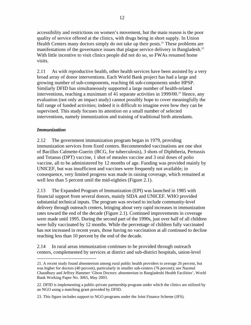
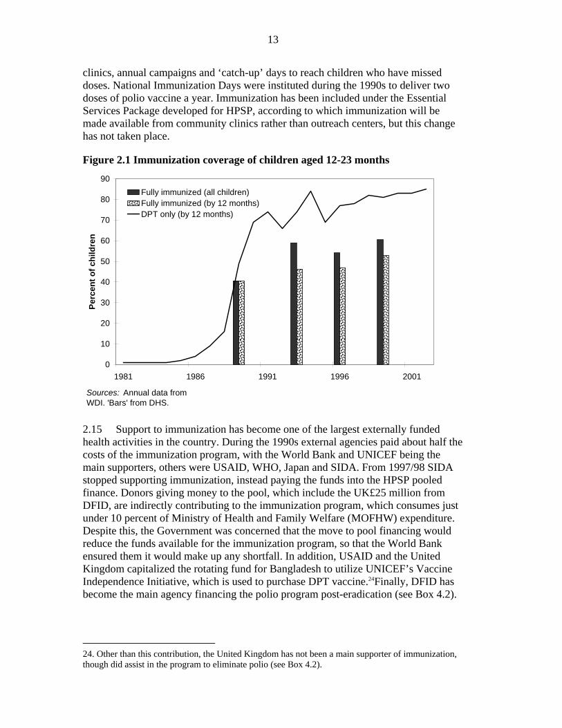
2.12 The government immunization program began in 1979, providing immunization services from fixed centers. Recommended vaccinations are one shot of Bacillus Calmette-Guerin (BCG, for tuberculosis), 3 shots of Diphtheria, Pertussis and Tetanus (DPT) vaccine, 1 shot of measles vaccine and 3 oral doses of polio vaccine, all to be administered by 12 months of age. Funding was provided mainly by UNICEF, but was insufficient and vaccines were frequently not available; in consequence, very limited progress was made in raising coverage, which remained at well less than 5 percent until the mid-eighties (Figure 2.1).

2.13 The Expanded Program of Immunization (EPI) was launched in 1985 with financial support from several donors, mainly SIDA and UNICEF. WHO provided substantial technical inputs. The program was revised to include community-level delivery through outreach centers, bringing about very rapid increases in immunization rates toward the end of the decade (Figure 2.1). Continued improvements in coverage were made until 1995. During the second part of the 1990s, just over half of all children were fully vaccinated by 12 months. While the percentage of children fully vaccinated has not increased in recent years, those having no vaccination at all continued to decline reaching less than 10 percent by the end of the decade.

2.14 In rural areas immunization continues to be provided through outreach centers, complemented by services at district and sub-district hospitals, union-level 21. A recent study found absenteeism among rural public health providers to average 26 percent, but was higher for doctors (40 percent), particularly in smaller sub-centers (76 percent); see Nazmul Chaudhury and Jeffrey Hammer ‘Ghost Doctors: absenteeism in Bangladeshi Health Facilities’, World Bank Working Paper No. 3065, May 2003.

22. DFID is implementing a public-private partnership program under which the clinics are utilized by an NGO using a matching grant provided by DFID.

23. This figure includes support to NGO programs under the Joint Finance Scheme (JFS).

13

clinics, annual campaigns and ‘catch-up’ days to reach children who have missed doses. National Immunization Days were instituted during the 1990s to deliver two doses of polio vaccine a year. Immunization has been included under the Essential Services Package developed for HPSP, according to which immunization will be made available from community clinics rather than outreach centers, but this change has not taken place.

Figure 2.1 Immunization coverage of children aged 12-23 months

0

10

20

30

40

50

60

70

80

90

1981 1986 1991 1996 2001

Perc

ent o

f chi

ldre

n

Fully immunized (all children)Fully immunized (by 12 months)DPT only (by 12 months)

Sources: Annual data from WDI. 'Bars' from DHS.

2.15 Support to immunization has become one of the largest externally funded health activities in the country. During the 1990s external agencies paid about half the costs of the immunization program, with the World Bank and UNICEF being the main supporters, others were USAID, WHO, Japan and SIDA. From 1997/98 SIDA stopped supporting immunization, instead paying the funds into the HPSP pooled finance. Donors giving money to the pool, which include the UK£25 million from DFID, are indirectly contributing to the immunization program, which consumes just under 10 percent of Ministry of Health and Family Welfare (MOFHW) expenditure. Despite this, the Government was concerned that the move to pool financing would reduce the funds available for the immunization program, so that the World Bank ensured them it would make up any shortfall. In addition, USAID and the United Kingdom capitalized the rotating fund for Bangladesh to utilize UNICEF’s Vaccine Independence Initiative, which is used to purchase DPT vaccine.24Finally, DFID has become the main agency financing the polio program post-eradication (see Box 4.2).

24. Other than this contribution, the United Kingdom has not been a main supporter of immunization, though did assist in the program to eliminate polio (see Box 4.2).

14

Training TBAs

2.16 During the 1990s traditional birth attendants attended over 60 percent of all births in Bangladesh, with their share increasing during the decade.25 Training of TBAs was, until recently, a central element of community-based health programs and an important part of strategies for safe motherhood. The World Bank and UNFPA trained around 14,000 TBAs in Bangladesh, the Bank doing so under HFP III and IV. However, in its decennial year (1997), the Safe Motherhood Initiative26 disavowed the approach. TBAs are mostly illiterate and so, it was argued, are little able to understand the training they receive. Drawing on international evidence, it was claimed that there was little or no evidence that training TBAs had any impact on maternal mortality – though the possible impact on neo-natal mortality (which is demonstrated below) received less attention. Hence the Safe Motherhood Initiative is now built around the objective of all births being attended by Skilled Birth Attendants -- explicitly excluding trained TBAs -- which has been included as an indicator for the Millennium Development Goals. Bangladesh has followed these international recommendations. Previous programs to train TBAs have been largely abandoned, with a new emphasis on making skilled attendants available.

Nutrition

2.17 While considerable progress had been made by the end of the 1980s in putting in place a family planning system, and areas of primary health were being developed, nutrition continued to suffer from neglect despite high levels of malnutrition. The Bangladesh National Nutrition Council was founded in 1975 to oversee nutrition policy and coordinate the various activities being undertaken by the different ministries. These activities included (1) subsidized food supplements to vulnerable population groups under the Ministry of Relief and Rehabilitation; (2) Homestead Garden Production implemented by the Ministry of Agriculture; (3) distribution of Vitamin A capsules twice a year to children aged 6 months to 6 years; and (4) iron and folic acid tablets for pregnant women distributed through satellite clinics. Several NGOs have been active in nutrition, notably the Bangladesh Rural Advancement Committee (BRAC) which was implementing a community-based nutrition project similar to that proposed by the Bank.

2.18 In place of this fragmented set of programs, the World Bank proposed a comprehensive approach to nutrition, at the heart of which was community-level nutritional counseling to encourage good nutritional practices amongst pregnant women and mothers of young children. A pilot program, the Bangladesh Integrated Nutrition Project (BINP), began in 6 thanas in 1996, expanding to 40 thanas by the time the project was completed in 2002. By that time the National Nutrition Program

25. The maternal mortality survey reported an even higher share of 74.4 percent of births being attended by TBAs (NIPORT et al, 2003: 52).

26. The Safe Motherhood Initiative is an international effort launched in Nairobi in 1987 which is supported by several international agencies, including the World Bank.

15

had begun, which is rolling the program out nationally. As a pilot project, BINP was subject to an intensive evaluation. These data are re-examined in Chapter 5.

16

3. Trends in Under-Five Mortality, Nutrition and Fertility

This chapter discusses trends in under-five mortality, nutrition and fertility. There is no dispute that mortality has fallen, and it is shown that the decline has benefited all population groups, although disparities remain. Nutrition has also improved, although, contrary to what is suggested by some data sources, reductions in malnutrition did not occur in the 1980s. Fertility has continued to decline during the 1990s, which is contrary to the picture suggested by the direct measures of the total fertility rate, which suggest a stagnation during the last decade.

Patterns of Mortality Decline

3.1 The decline in under-five mortality has benefited all groups of the population, by age, wealth, gender and location. But disparities between boys and girls, and different regions of the country, remain high. This section examines these patterns using data from the three DHS surveys.

3.2 From 1985-89 to 1995-99 mortality among the under-fives fell by close to 40 percent, from over 150 deaths per 1,000 live births to less than 100 (Figure 1.1). This decline took place for all age groups -- neonates as well as children aged 1-527 -- and all income groups. Indeed, during the 1990s under-five mortality fell marginally faster for the poor than the non-poor.28

3.3 However, there is a sex-bias in Bangladeshi mortality rates. In most countries, boy children are more likely to die between their first and fifth birthdays than are girls. Bangladesh is an exception to this pattern: girl children aged 1 to 4 years are thirty-three percent more likely to die than are boy children. This is one of the highest female-male child mortality ratios in the world.29

27. The usual pattern is that mortality falls much more rapidly for older children, so that the remaining deaths become concentrated first among infants and, within that category, among neonates (and indeed within neonates to the first days of life being the most risky). This pattern is less marked in Bangladesh than elsewhere, with neonatal mortality falling as fast as that for post-nates (up to one month), and not too far behind that of children (1 to 4 years).

28. The poor are identified as the bottom 50 percent, ranked by a wealth index, in the 1992/93 DHS data. The wealth index poverty line from that survey was applied to the subsequent surveys so that data are comparable between years. This conclusion is robust to the choice of the poverty line; the concentration curve for the early 1990s has first order dominance over that for the late nineties up to around the seventh decile. Analysis shows that within group reductions of mortality accounted for far more of the fall in mortality than did movements out of poverty (i.e. into a lower mortality group); see appendix C.3.

29. Data were examined from 125 DHS surveys. Ranking these surveys by female:male mortality in descending order, the ratio from the three Bangladesh surveys rank 8th, 9th and 12th, i.e. in the worst 10 percent. There is no gender bias in neo-natal mortality, with girls less likely to die than boys in the first month of life. A bias begins to emerge for post-natal mortality, though not as marked as that for child mortality.

17

3.4 Marked regional variations in life chances also persist. A child is twice as likely to die before reaching their fifth birthday in Sylhet as he or she -- but particularly she -- is in Khulna.

Anthropometric Outcomes

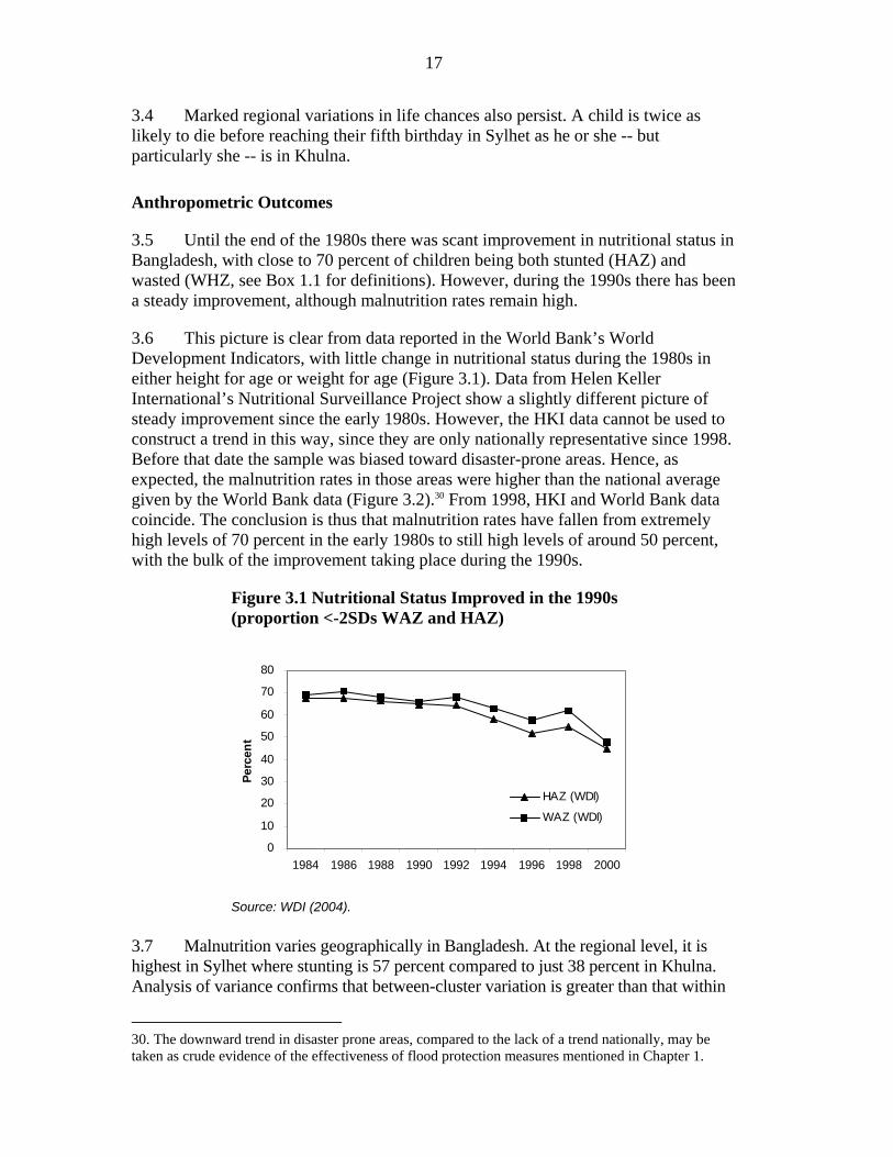
3.5 Until the end of the 1980s there was scant improvement in nutritional status in Bangladesh, with close to 70 percent of children being both stunted (HAZ) and wasted (WHZ, see Box 1.1 for definitions). However, during the 1990s there has been a steady improvement, although malnutrition rates remain high.

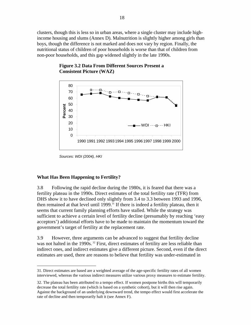
3.6 This picture is clear from data reported in the World Bank’s World Development Indicators, with little change in nutritional status during the 1980s in either height for age or weight for age (Figure 3.1). Data from Helen Keller International’s Nutritional Surveillance Project show a slightly different picture of steady improvement since the early 1980s. However, the HKI data cannot be used to construct a trend in this way, since they are only nationally representative since 1998. Before that date the sample was biased toward disaster-prone areas. Hence, as expected, the malnutrition rates in those areas were higher than the national average given by the World Bank data (Figure 3.2).30 From 1998, HKI and World Bank data coincide. The conclusion is thus that malnutrition rates have fallen from extremely high levels of 70 percent in the early 1980s to still high levels of around 50 percent, with the bulk of the improvement taking place during the 1990s.

Figure 3.1 Nutritional Status Improved in the 1990s (proportion <-2SDs WAZ and HAZ)

0

10

20

30

40

50

60

70

80

1984 1986 1988 1990 1992 1994 1996 1998 2000

Perc

ent

HAZ (WDI)

WAZ (WDI)

Source: WDI (2004).

3.7 Malnutrition varies geographically in Bangladesh. At the regional level, it is highest in Sylhet where stunting is 57 percent compared to just 38 percent in Khulna. Analysis of variance confirms that between-cluster variation is greater than that within

30. The downward trend in disaster prone areas, compared to the lack of a trend nationally, may be taken as crude evidence of the effectiveness of flood protection measures mentioned in Chapter 1.

18

clusters, though this is less so in urban areas, where a single cluster may include high-income housing and slums (Annex D). Malnutrition is slightly higher among girls than boys, though the difference is not marked and does not vary by region. Finally, the nutritional status of children of poor households is worse than that of children from non-poor households, and this gap widened slightly in the late 1990s.

Figure 3.2 Data From Different Sources Present a Consistent Picture (WAZ)

01020304050607080

1990 1991 1992 19931994 1995 19961997 1998 1999 2000

Perc

ent

WDI HKI

Sources: WDI (2004), HKI

What Has Been Happening to Fertility?

3.8 Following the rapid decline during the 1980s, it is feared that there was a fertility plateau in the 1990s. Direct estimates of the total fertility rate (TFR) from DHS show it to have declined only slightly from 3.4 to 3.3 between 1993 and 1996, then remained at that level until 1999.31 If there is indeed a fertility plateau, then it seems that current family planning efforts have stalled. While the strategy was sufficient to achieve a certain level of fertility decline (presumably by reaching ‘easy acceptors’) additional efforts have to be made to maintain the momentum toward the government’s target of fertility at the replacement rate.

3.9 However, three arguments can be advanced to suggest that fertility decline was not halted in the 1990s. 32 First, direct estimates of fertility are less reliable than indirect ones, and indirect estimates give a different picture. Second, even if the direct estimates are used, there are reasons to believe that fertility was under-estimated in

31. Direct estimates are based are a weighted average of the age-specific fertility rates of all women interviewed, whereas the various indirect measures utilize various proxy measures to estimate fertility.

32. The plateau has been attributed to a tempo effect. If women postpone births this will temporarily decrease the total fertility rate (which is based on a synthetic cohort), but it will then rise again. Against the background of an underlying downward trend, the tempo effect would first accelerate the rate of decline and then temporarily halt it (see Annex F).

19

1993/94 on account of displacement in birth reporting. Third, if indirect estimates are used, they show both that the direct estimates under-estimate fertility (particularly in 1993/94, reinforcing the previous point) and that fertility did continue to decline in the 1990s. These arguments are considered in turn.

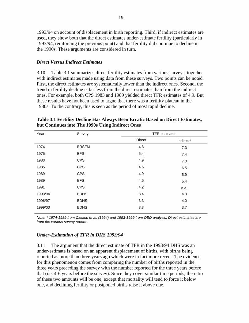
Direct Versus Indirect Estimates

3.10 Table 3.1 summarizes direct fertility estimates from various surveys, together with indirect estimates made using data from these surveys. Two points can be noted. First, the direct estimates are systematically lower than the indirect ones. Second, the trend in fertility decline is far less from the direct estimates than from the indirect ones. For example, both CPS 1983 and 1989 yielded direct TFR estimates of 4.9. But these results have not been used to argue that there was a fertility plateau in the 1980s. To the contrary, this is seen as the period of most rapid decline.

Table 3.1 Fertility Decline Has Always Been Erratic Based on Direct Estimates, but Continues into The 1990s Using Indirect Ones

TFR estimates Year Survey

Direct Indirect* 1974 BRSFM 4.8 7.3 1975 BFS 5.4 7.4 1983 CPS 4.9 7.0 1985 CPS 4.6 6.5 1989 CPS 4.9 5.9 1989 BFS 4.6 5.4 1991 CPS 4.2 n.a. 1993/94 BDHS 3.4 4.3

1996/97 BDHS 3.3 4.0

1999/00 BDHS 3.3 3.7

Note: * 1974-1989 from Cleland et al. (1994) and 1993-1999 from OED analysis. Direct estimates are from the various survey reports.

Under-Estimation of TFR in DHS 1993/94

3.11 The argument that the direct estimate of TFR in the 1993/94 DHS was an under-estimate is based on an apparent displacement of births, with births being reported as more than three years ago which were in fact more recent. The evidence for this phenomenon comes from comparing the number of births reported in the three years preceding the survey with the number reported for the three years before that (i.e. 4-6 years before the survey). Since they cover similar time periods, the ratio of these two amounts will be one, except that mortality will tend to force it below one, and declining fertility or postponed births raise it above one.

20

3.12 But this ratio for the 1993/94 survey is greatly in excess of both one and the value of the ratio observed in the other surveys. In the earlier survey, 26 percent more births were reported for 4-6 years before the survey compared to within three years before the survey. This ratio compares with just 4 percent for 1996/97 and a five percent reduction in 1999/00. Yet comparing the ratio for five-year periods there is little difference between the1993/94 and 1996/97 surveys. These data thus show that in 1993/94 children under three were being reported as being older. The effect of this birth displacement is exactly the same as for the postponement of births. That is, it will reduce the reported total fertility rate. But since, in this case, the reduction comes from incorrectly attributing births to a later period there is a downward bias of the direct fertility estimate for 1993/94.

Indirect fertility measures

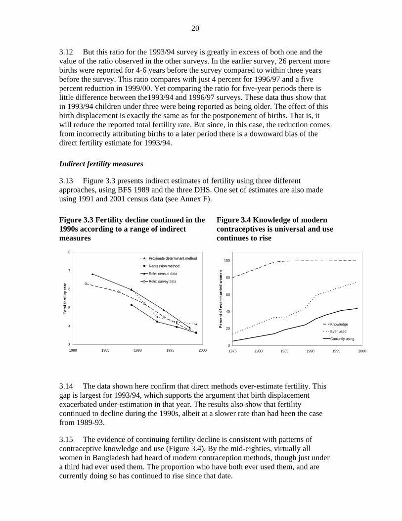
3.13 Figure 3.3 presents indirect estimates of fertility using three different approaches, using BFS 1989 and the three DHS. One set of estimates are also made using 1991 and 2001 census data (see Annex F).

Figure 3.3 Fertility decline continued in the 1990s according to a range of indirect measures

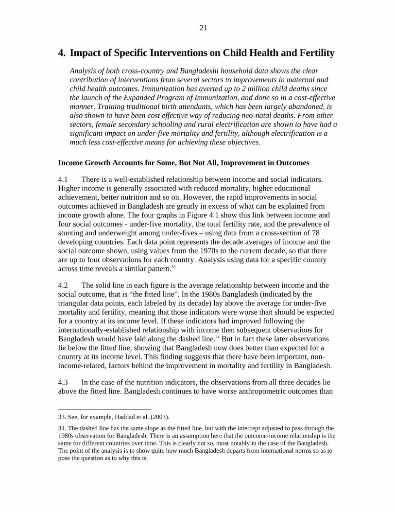
Figure 3.4 Knowledge of modern contraceptives is universal and use continues to rise

3

4

5

6

7

8

1980 1985 1990 1995 2000

Tota

l fer

tility

rate

Proximate determinant method

Regression method

Rele: census data

Rele: survey data

0

20

40

60

80

100

1975 1980 1985 1990 1995 2000

Perc

ent o

f eve

r-m

arrie

d w

omen

Knowledge

Ever used

Currently using

3.14 The data shown here confirm that direct methods over-estimate fertility. This gap is largest for 1993/94, which supports the argument that birth displacement exacerbated under-estimation in that year. The results also show that fertility continued to decline during the 1990s, albeit at a slower rate than had been the case from 1989-93.

3.15 The evidence of continuing fertility decline is consistent with patterns of contraceptive knowledge and use (Figure 3.4). By the mid-eighties, virtually all women in Bangladesh had heard of modern contraception methods, though just under a third had ever used them. The proportion who have both ever used them, and are currently doing so has continued to rise since that date.

21

4. Impact of Specific Interventions on Child Health and Fertility

Analysis of both cross-country and Bangladeshi household data shows the clear contribution of interventions from several sectors to improvements in maternal and child health outcomes. Immunization has averted up to 2 million child deaths since the launch of the Expanded Program of Immunization, and done so in a cost-effective manner. Training traditional birth attendants, which has been largely abandoned, is also shown to have been cost effective way of reducing neo-natal deaths. From other sectors, female secondary schooling and rural electrification are shown to have had a significant impact on under-five mortality and fertility, although electrification is a much less cost-effective means for achieving these objectives.

Income Growth Accounts for Some, But Not All, Improvement in Outcomes

4.1 There is a well-established relationship between income and social indicators. Higher income is generally associated with reduced mortality, higher educational achievement, better nutrition and so on. However, the rapid improvements in social outcomes achieved in Bangladesh are greatly in excess of what can be explained from income growth alone. The four graphs in Figure 4.1 show this link between income and four social outcomes - under-five mortality, the total fertility rate, and the prevalence of stunting and underweight among under-fives – using data from a cross-section of 78 developing countries. Each data point represents the decade averages of income and the social outcome shown, using values from the 1970s to the current decade, so that there are up to four observations for each country. Analysis using data for a specific country across time reveals a similar pattern.33

4.2 The solid line in each figure is the average relationship between income and the social outcome, that is “the fitted line”. In the 1980s Bangladesh (indicated by the triangular data points, each labeled by its decade) lay above the average for under-five mortality and fertility, meaning that those indicators were worse than should be expected for a country at its income level. If these indicators had improved following the internationally-established relationship with income then subsequent observations for Bangladesh would have laid along the dashed line.34 But in fact these later observations lie below the fitted line, showing that Bangladesh now does better than expected for a country at its income level. This finding suggests that there have been important, non-income-related, factors behind the improvement in mortality and fertility in Bangladesh.

4.3 In the case of the nutrition indicators, the observations from all three decades lie above the fitted line. Bangladesh continues to have worse anthropometric outcomes than

33. See, for example, Haddad et al. (2003).

34. The dashed line has the same slope as the fitted line, but with the intercept adjusted to pass through the 1980s observation for Bangladesh. There is an assumption here that the outcome-income relationship is the same for different countries over time. This is clearly not so, most notably in the case of the Bangladesh. The point of the analysis is to show quite how much Bangladesh departs from international norms so as to pose the question as to why this is.

22

the average for countries at a similar income level. But this discrepancy has narrowed over time. The improvement in all four outcomes greatly exceeds that in GNP per capita, and exceeds the expected improvement derived for growth in national income.

Figure 4.1 Bangladesh’s improvement in social outcomes is greater than can be explained by economic growth alone

(a) Under-five mortality (b) Total fertility rate

0

50

100

150

200

250

300

350

400

0 2000 4000 6000 8000 10000 12000 14000 16000 18000

GDP per capita (US$)

Und

er fi

ve m

orta

lity

(per

000

live

birt

hs)

1980s

1990s

2000

Fitted line

Income-driven trajectory

0

1

2

3

4

5

6

7

8

9

0 2000 4000 6000 8000 10000 12000 14000 16000 18000

GDP per capita (US$)To

tal F

ertil

ity R

ate 1980s

1990s

2000sFitted line

Income driven trajectory

(c) Stunting (height for age)

(d) Underweight (weight for age)

0

10

20

30

40

50

60

70

80

90

0 2000 4000 6000 8000 10000 12000 14000 16000 18000


Stun

ting

(hei

ght f

or a

ge)

1980s

1990s

2000

Fitted line


-10

0

10

20

30

40

50

60

70

80

90

0 2000 4000 6000 8000 10000 12000 14000 16000 180


Und

erw

eigh

t (w

eigh

t for

age

)

1980s

1990s

2000

Fitted line


Note: See discussion in paras. 4.1-4.3 for explanation.

Table 4.1 Growth in GNP Per Capita Accounts for at Most One-Third of The Reduction in Mortality… and Less Than a Fifth of Lower Fertility

1980 actual 2000 actual 2000 income-based estimate

Percent reduction explained by income

Under-five mortality 205.0 77.5 163.1 32.9 Total fertility rate 5.6 3.0 5.2 16.0 Stunting 67.6 44.7 62.3 23.1 Underweight 69.5 47.7 64.6 22.4

Source: calculated from data used for Figure 4.1 (see Annex B) 4.4 The numbers behind these graphs provide an upper estimate of the extent to which growth in GDP per capita has contributed to improved social outcomes in

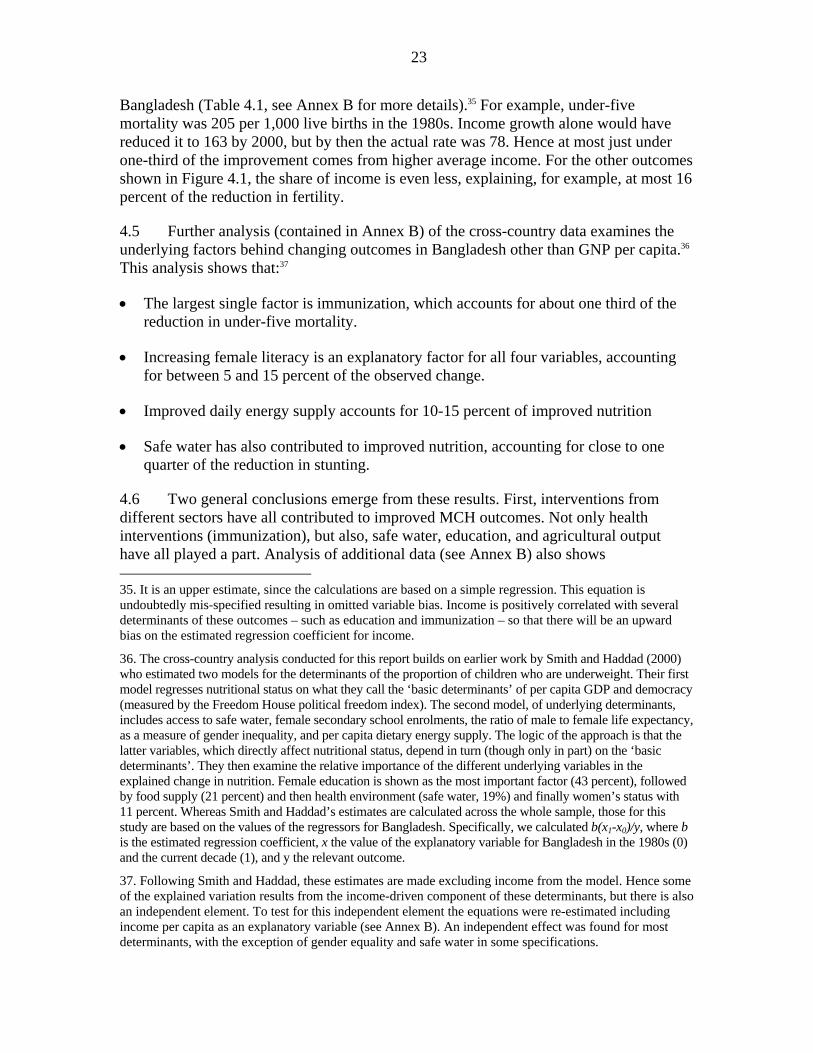
23

Bangladesh (Table 4.1, see Annex B for more details).35 For example, under-five mortality was 205 per 1,000 live births in the 1980s. Income growth alone would have reduced it to 163 by 2000, but by then the actual rate was 78. Hence at most just under one-third of the improvement comes from higher average income. For the other outcomes shown in Figure 4.1, the share of income is even less, explaining, for example, at most 16 percent of the reduction in fertility.

4.5 Further analysis (contained in Annex B) of the cross-country data examines the underlying factors behind changing outcomes in Bangladesh other than GNP per capita.36 This analysis shows that:37

• The largest single factor is immunization, which accounts for about one third of the reduction in under-five mortality.

• Increasing female literacy is an explanatory factor for all four variables, accounting for between 5 and 15 percent of the observed change.

• Improved daily energy supply accounts for 10-15 percent of improved nutrition

• Safe water has also contributed to improved nutrition, accounting for close to one quarter of the reduction in stunting.

4.6 Two general conclusions emerge from these results. First, interventions from different sectors have all contributed to improved MCH outcomes. Not only health interventions (immunization), but also, safe water, education, and agricultural output have all played a part. Analysis of additional data (see Annex B) also shows 35. It is an upper estimate, since the calculations are based on a simple regression. This equation is undoubtedly mis-specified resulting in omitted variable bias. Income is positively correlated with several determinants of these outcomes – such as education and immunization – so that there will be an upward bias on the estimated regression coefficient for income.

36. The cross-country analysis conducted for this report builds on earlier work by Smith and Haddad (2000) who estimated two models for the determinants of the proportion of children who are underweight. Their first model regresses nutritional status on what they call the ‘basic determinants’ of per capita GDP and democracy (measured by the Freedom House political freedom index). The second model, of underlying determinants, includes access to safe water, female secondary school enrolments, the ratio of male to female life expectancy, as a measure of gender inequality, and per capita dietary energy supply. The logic of the approach is that the latter variables, which directly affect nutritional status, depend in turn (though only in part) on the ‘basic determinants’. They then examine the relative importance of the different underlying variables in the explained change in nutrition. Female education is shown as the most important factor (43 percent), followed by food supply (21 percent) and then health environment (safe water, 19%) and finally women’s status with 11 percent. Whereas Smith and Haddad’s estimates are calculated across the whole sample, those for this study are based on the values of the regressors for Bangladesh. Specifically, we calculated b(x1-x0)/y, where b is the estimated regression coefficient, x the value of the explanatory variable for Bangladesh in the 1980s (0) and the current decade (1), and y the relevant outcome.

37. Following Smith and Haddad, these estimates are made excluding income from the model. Hence some of the explained variation results from the income-driven component of these determinants, but there is also an independent element. To test for this independent element the equations were re-estimated including income per capita as an explanatory variable (see Annex B). An independent effect was found for most determinants, with the exception of gender equality and safe water in some specifications.

24

electrification to be a fairly robust determinant of mortality outcomes. Second, there is a residual (unexplained) element in these figures, most notably for weight for age and the fertility rate. The remainder of this chapter builds on these results to further analyze the factors behind improved MCH outcomes in Bangladesh and the extent to which public interventions have brought about these improvements.

Under-five Mortality

4.7 The reasons for premature death vary by age. For very young children, factors related to maternal health during pregnancy and the birth itself are important, with other aspects of health care mattering throughout infancy. But for children aged more than one year, the general socio-economic environment matters more. It is thus common to analyze mortality determinants separately for the different age groups. Such an analysis was conducted by OED using DHS data from the three surveys carried out in the 1990s (see Annex C for detailed results).

4.8 Table 4.2 summarizes the significant determinants of the mortality for the different age groups as revealed by OED’s analysis. The main findings are:

• Mother’s education matters, though it must be to at least secondary level to affect infant mortality. Mother’s contraceptive knowledge is included as a proxy for maternal health knowledge, and exerts a significant impact for infants but not children. Other measures of women’s agency have some effect, notably the greater mortality risk for children of women who have remarried.

• Money matters, though not for neonatal mortality. • Various factors correlated to fertility influence mortality: there is a non-linear

relationship between mother’s age and infant mortality, with the probability of premature death decreasing until close to age 30, after which it increases again. For children there is a simpler relationship: children born to older mothers have less chance of dying. A short birth interval adversely affects mortality. The pattern for birth order is more complex: lower order births, particularly the first-born child, are at greater risk, though this risk is mitigated slightly if the mother attends antenatal care. The data suggest that the risk of mortality for infants declines with birth order until a birth order of six, after which it rises again.

• Sex bias manifests itself in various ways. Female children are more likely to die than male, especially those in Chittagong38 and those of a higher birth order.

• The health and nutrition related variables have the expected positive impact.39 Immunization is dealt with in detail below. Antenatal visits reduce neo-natal mortality, but only if provided by trained medical personnel, either doctor or

38. Bangladesh has six divisions: Barisal, Chittagong, Dhaka, Khulna, Rajshahi and Sylhet. Sylhet was formerly part of Chittagong, so that Chittagong (including Sylhet) is used for the regional analysis.

39. Many care-related variables are difficult to include for reasons of endogeneity. Controlling for endogeneity of antenatal care shows it to only be significant if provided by a trained doctor or nurse. It is not possible to include breastfeeding in the equations as the only available question (never breastfeed) is a function of child health.

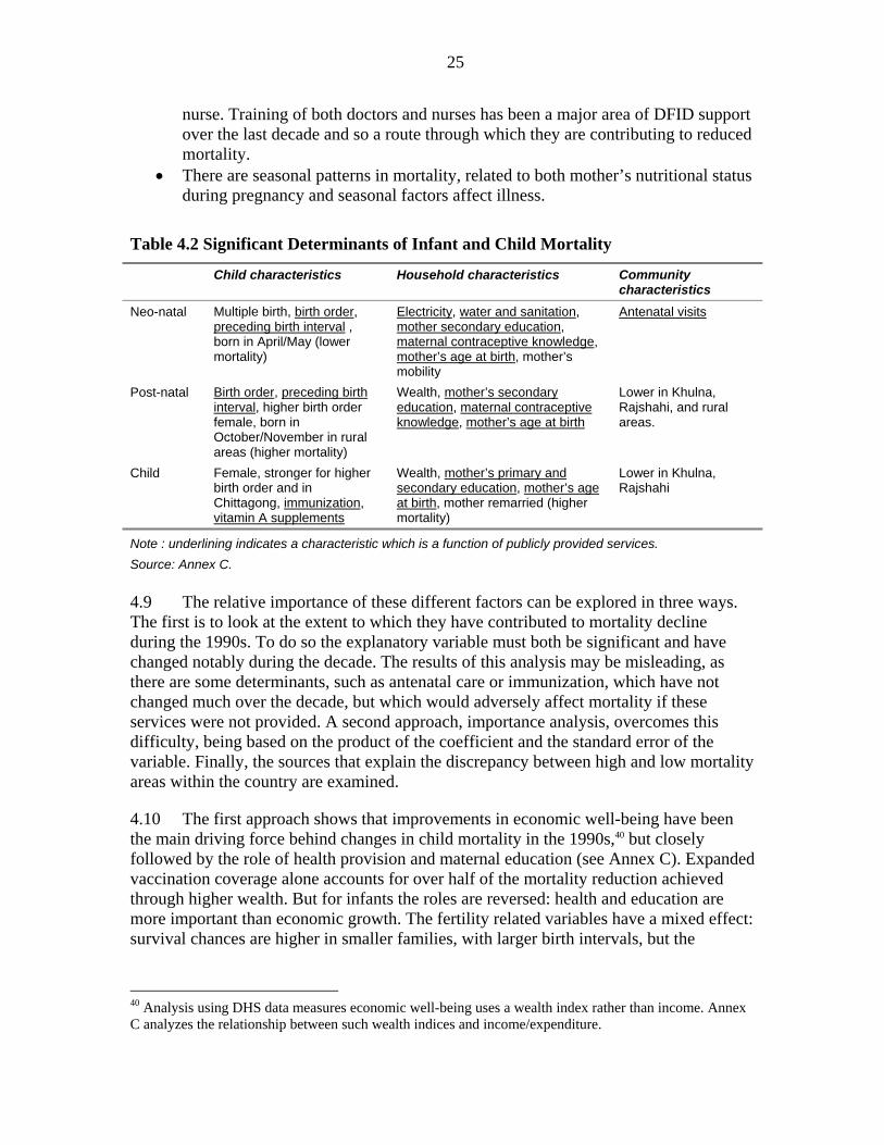
25

nurse. Training of both doctors and nurses has been a major area of DFID support over the last decade and so a route through which they are contributing to reduced mortality.

• There are seasonal patterns in mortality, related to both mother’s nutritional status during pregnancy and seasonal factors affect illness.

Table 4.2 Significant Determinants of Infant and Child Mortality

Child characteristics Household characteristics Community characteristics

Neo-natal Multiple birth, birth order, preceding birth interval , born in April/May (lower mortality)

Electricity, water and sanitation, mother secondary education, maternal contraceptive knowledge, mother’s age at birth, mother’s mobility

Antenatal visits

Post-natal Birth order, preceding birth interval, higher birth order female, born in October/November in rural areas (higher mortality)

Wealth, mother’s secondary education, maternal contraceptive knowledge, mother’s age at birth

Lower in Khulna, Rajshahi, and rural areas.

Child Female, stronger for higher birth order and in Chittagong, immunization, vitamin A supplements

Wealth, mother’s primary and secondary education, mother’s age at birth, mother remarried (higher mortality)

Lower in Khulna, Rajshahi

Note : underlining indicates a characteristic which is a function of publicly provided services. Source: Annex C. 4.9 The relative importance of these different factors can be explored in three ways. The first is to look at the extent to which they have contributed to mortality decline during the 1990s. To do so the explanatory variable must both be significant and have changed notably during the decade. The results of this analysis may be misleading, as there are some determinants, such as antenatal care or immunization, which have not changed much over the decade, but which would adversely affect mortality if these services were not provided. A second approach, importance analysis, overcomes this difficulty, being based on the product of the coefficient and the standard error of the variable. Finally, the sources that explain the discrepancy between high and low mortality areas within the country are examined.

4.10 The first approach shows that improvements in economic well-being have been the main driving force behind changes in child mortality in the 1990s,40 but closely followed by the role of health provision and maternal education (see Annex C). Expanded vaccination coverage alone accounts for over half of the mortality reduction achieved through higher wealth. But for infants the roles are reversed: health and education are more important than economic growth. The fertility related variables have a mixed effect: survival chances are higher in smaller families, with larger birth intervals, but the

40 Analysis using DHS data measures economic well-being uses a wealth index rather than income. Annex C analyzes the relationship between such wealth indices and income/expenditure.

26

reduction in birth order tends to increase mortality.41 The importance analysis bears out these results, showing in particular the role of health and education. Two factors mainly explain why mortality outcomes are so much better in Khulna than Chittagong: (1) differing rates of accessing health services, and (2) pronounced excess female mortality in Chittagong, which is not present in Khulna.42

4.11 The above analysis of determinants is now used to quantify the impact and cost effectiveness of the following interventions: immunization, training TBAs, female secondary schooling and rural electrification.

Immunization

4.12 Immunization in Bangladesh has expanded greatly in the last two decades (see Chapter 2 and Box 4.1). Both improvements in socio-economic conditions and immunization reduce disease. A disease such as polio spreads more easily where access to safe water is limited, so that improving water supply can reduce incidence. But eradication of the disease requires a coordinated public health strategy, as has been implemented in Bangladesh with external assistance (see Box 4.2).

41. First born children have a higher risk of infant death than do subsequent births. Lowering fertility means increasing the proportion of first born children, exerting an upward influence on infant mortality.

42. When interacting the female dummy with the Chittagong dummy, the female dummy is no longer significant, but that for the interactive term significantly positive.

Box 4.1 Which Children Get Immunized?

Bangladesh’s immunization program took off in the second half of the 1980s, rapidly expanding coverage. Despite this expansion, close to half of all children do not receive the full course of recommended vaccinations, and a significant number remain unvaccinated.

Multivariate analysis of DHS data shows the following:

• Several variables related to women’s position (see Annex E for discussion of measures and correlates of women’s agency) have a significant impact on the likelihood of a child being vaccinated: mother’s age, mobility, agency and education. Children of mothers who have remarried are less likely to be vaccinated.

• The divisional disadvantage of Dhaka, Sylhet and Chittagong remains significant even once the other factors mentioned are controlled for. And the advantage of Khulna and Rajshahi is also significant. Distance from thana headquarters (HQ) reduces the likelihood of a child being immunized.

• Electricity has a significant positive impact. Two indirect channels for electrification – wealth and access to information (TV) – are already included, as is a locational variable (distance to thana HQ) which electrification may proxy for. Hence the result most likely reflects at least in part the impact of electrification on preserving the cold chain (keeping vaccines at the required temperature).

• Wealth has a positive but statistically insignificant impact on the probability of being immunized.

These results point to the importance of information campaigns in overcoming remaining barriers to immunization. As discussed elsewhere in this report (Chapter 5), the message at the heart of behavior change communication – that all actors in the decision-making process need be reached – needs to be born in mind.

27

4.13 More generally, there are various ways in which the deaths averted by immunization may be calculated (see Annex C for details on the calculations):

• The cross-country regression analysis undertaken for this study (Annex B) suggests that increased immunization coverage accounts for close to one-third of the reduction in under-five mortality over the past two decades. Immunization began to rise from the mid-80s. If mortality had remained at its 1987 level, there would have been 3.28 million additional under-five deaths from 1987-2002: just under one million of these lives saved being attributable to immunization.

• A study conducted in the late 1990s considered the life-saving effects of each vaccination separately, producing an estimate of 1.15 million deaths prevented in the period 1987-98 (Khan and Yoder, 1998).

• The child mortality regressions show that children with no vaccinations are between 50 percent to twice as likely to die as those children who have some coverage.43 Applying this ratio to observed mortality data suggests that over 2 million child deaths have been averted by immunization between 1981 and 2002 (see Annex C for details).

Box 4.2 Polio Eradication in Bangladesh

Polio is a viral disease which affects the nervous system, muscles and can cause paralysis. Children under three are most at risk. The disease is transmitted by physical contact, and is highly contagious in areas with poor sanitation and high population density – making areas of Bangladesh very vulnerable. But polio is easily preventable using inexpensive vaccines.

In 1988 the World Health Assembly of WHO set the goal of the global eradication of polio by year 2000. There has been considerable progress toward this goal. In 1988 there were 350,000 cases every year worldwide. In 2003 the number had dropped to 1,000. Only 6 countries still have endemic polio: Afghanistan, India, Pakistan, Niger, Nigeria and Egypt.

Bangladesh has tackled polio through the four strategies identified by WHO: routine immunization as a part of EPI, National Immunization Days (NIDs), a surveillance system to identify outbreaks and a mopping up strategy in case polio re-appears in any location. This strategy in Bangladesh has been very successful. Before 1986 an estimated 11,500 children developed polio every year. This number was reduced to 2,300 in 1994 and 324 in 1999. Since 2000 no polio cases have been identified.

Funding efforts have been coordinated internationally by the Global Polio Eradication Initiative, which includes WHO, UNICEF, Rotary International, USAID and other donors. In Bangladesh nearly 50 percent of the funding has been provided by the government of Japan, that spent around 40-50 million dollars in NIDS up to 2003. Other large donors are CDC and Rotary (10% each), other minor donors follow: UNICEF (6%), WHO (3%), USAID (3%), DFID (2%), etc. However, since eradication, DFID has expanded its support with a UK$7 million project ‘Support to Polio Eradication’, under which coverage through NIDS is approaching 100 percent (97% in 2004). Sources: WHO/CDC/UNICEF (2004), Polio eradication website, http://www.polioeradication.org/; and CDC (various issues), Morbidity and Mortality Weekly Report

43. The hazard ratio for the Cox regression using 1999 data was 2.05 (Annex C.3). Using pooled data, and a without-self mean of immunization to account for potential endogeneity, the ratio falls to 1.55.

28

4.14 These differing approaches give somewhat different estimates of the number of lives saved by EPI, but provide a range of one to two million deaths averted, which can be used as a basis for cost effectiveness analysis. There are also wide estimates of the full cost of immunizing a child. A study on immunization in Bangladesh in the late 1990s reported a figure of close to US$12 per child, a little less than international norms.44 The study also presents the direct costs of the EPI program and estimates of total costs, i.e. including staff and equipment costs not reflected in the EPI budget, for a single year (US$18.3 million in 1997/98). Applying these figures gives a range of the cost per life saved from just under $100 to just under $300.45 The OED analysis thus confirms the relatively low cost of immunization as a means of saving lives.46 These figures are likely to be an under-estimate since they ignore the benefits of herd immunity, which is yet to be realized in Bangladesh.47

4.15 The number of deaths averted can be attributed to the agencies supporting the immunization program on a pro rata basis. The World Bank has contributed approximately 10 percent of program costs over the last 15 years, thus saving the lives of between 100,000 and 200,000 Bangladeshi children. DFID’s contribution to immunization has been mainly to the polio program since eradication. Before the polio eradication campaign over 10,000 children a year were developing the disease, which gives an indication of the benefits from keeping the disease from re-appearing.

Trained TBAs

4.16 As described in Chapter 2, Bangladesh followed international trends in abandoning training of TBAs. But the international evidence is more nuanced than this wholesale shift in focus suggests. First, studies are clear that training TBAs does make a difference to their behavior. For example, a study in Bangladesh found that 45 percent of trained TBAs practiced the ‘three cleans’ (hand-washing with soap, clean cord care, clean surface) compared to 19 percent of untrained TBAs (Goodburn et al., 2000: 396; and see Sibley et al., 2004 for results of a meta-analysis). Moreover, there have been cases of substantial reductions in maternal mortality in systems relying on trained TBAs, when backed up by a good referral system for Emergency Obstetric Care (EOC): China being the best known case,48 and Bangladesh cited as one in which there was no such system of

44. Khan, M.M. and Yoder, R.A. (1998) “Expanded Program on Immunization in Bangladesh: Cost, Cost-Effectiveness, and Financing Estimates” Special Initiatives Report No. 6, Partnerships for Health Reform, Bethesda MD. The Bangladesh EPI office currently report a figure of $10 per child.

45. Khan and Yoder (1998) arrive at an estimate of US$136 per life saved.

46. Moreover, the cost of treatment of children who become sick can be shown to exceed the cost of avoiding sickness so that immunization represents a saving of health expenditures.

47. Once immunization reaches a certain threshold then there is a reduction in the cross-infection, so that unimmunized children are also less at risk of the disease. The threshold varies by disease but is mostly in the range 80-90 percent (Fine, 1993).

48. In China between 1950 and 1980 maternal mortality ratio declined from 1500 to 115 per 100,000 live births. The vast majority of births during this period were delivered by minimally trained village birth attendants (backed up by a strong obstetric care and emergency referral network) (Levitt, 1999).

29

EOC and, consequently, no impact on maternal deaths.49 Finally, while there is no evidence of an impact on maternal mortality, there is evidence of an impact on infant mortality. The meta-analysis of the impact of training TBAs reported that 14 out of 17 studies found a reduction of peri-neonatal mortality from births being attended by trained, rather than untrained, TBAs (Sibley et al., 2004).

4.17 Turning to the Bangladeshi data, training TBAs appears to have a beneficial impact on neo-natal mortality, though there are complications in interpreting these figures. Table 4.3 shows the share of births attended by trained and untrained TBAs from each DHS, and the neo-natal mortality rate for births so attended. The existence of training programs for TBAs is evident from the expansion of the share of births attended by trained TBAs (TTBAs) from 4 to 10 percent between 1993 and 1999. At the same time the neonatal mortality rate among births to trained TBAs has more than halved – a much larger fall than that observed in general or among births attended by untrained TBAs.

Table 4.3. Neo-natal Mortality Has Fallen Much More Rapidly for Births Attended by Trained TBAs

Percent of deliveries Neo-natal mortality

(per 1,000 live births)

Untrained Trained Untrained Trained

1993 55.0 4.3 49 72

1996 56.7 7.6 48 49

1999 53.2 9.5 38 31

4.18 But various factors complicate the picture.50 Trained TBAs are likely to attend more difficult births than untrained TBAs, as is evident from the higher mortality rate for these births in 1993.51 As training for TBAs expands, so that trained TBAs are more widespread, this effect may be diluted, thus driving down mortality associated with TTBA-attended birth. Second, the training encourages TBAs to refer difficult births to EOC. Partly in consequence, the share of births attended by doctors also increased during this period, though this was mainly in urban areas (i.e. only for a minority of births). This effect will also reduce the mortality associated with trained TBAs. Finally, training may

49. However, the study of Goodland et al. (2002) finds that training TBAs did not reduce postpartum infection, which they attribute to the importance of pre-existing reproductive tract infection. This is not something to which EOC would have made a difference.

50. Multivariate analysis suffers from the same problems illustrated in the bivariate analysis (Table 4.3). That is, in the neonatal mortality regression, the coefficient for births attended by trained TBAs is significantly positive (that for untrained TBAs is significantly negative), but the interaction of the year with trained TBA is negative, and of sufficient magnitude to give trained TBAs an advantage over untrained by 1999. This result remains when a trivariate probit is estimated (to handle the endogeneity of ante-natal care and choice of birth attendant). The trivariate results show which women use TTBAs: the coefficient for the later period is highly significant, picking up the increased availability of TTBAs, so is being a female household head, a multiple birth, having attended ANC and the mother’s age.

51. This issue of difficult birth selectivity is yet more severe for births at health facilities, making it very difficult to measure the beneficial impact of such facilities by this sort of statistical analysis.

30

reduce mortality owing to greater skills of TBAs who are trained, which is what is hoped to be observed, but difficult to disentangle from the other factors described above. However, it can be observed that neonatal mortality among babies whose birth was attended by a trained TBA was, in 1999, lower than that for untrained TBAs, despite the continued presence of the greater likelihood of difficult births for trained TBAs, which strongly suggests that training TBAs had a beneficial impact on neo-natal mortality.

4.19 An estimate of the advantage of training is given by the single difference impact of 7 deaths averted per 1,000 live births.52 The coefficients from the multivariate analysis suggest a double difference impact of 5 per 1,000. These figures are consistent with the meta-analysis mentioned in paragraph 4.16, which found that training TBAs reduced peri-neonatal mortality by 7 per 1,000 (Sibley et al., 2004). The cost of training a single TBA is in the range US$350-400, and one TBA attends between 10-15 births a year.53 Hence training one TBA saves 0.05-0.105 lives per year, suggesting a cost of between US$3,300-8,000 per life saved each year. The TBA may continue to practice using this knowledge for between 10-15 years after training, bringing the cost per life saved down to US$220-800. These figures show training TBAs to be a cost effective strategy for tackling infant mortality.

4.20 In a setting where 60-75 percent of births are attended by TBAs it is not prudent to sideline them in any strategy for improving health outcomes. Doing so in Bangladesh was the result of faddism on the part of the international community, rather than a decision based on solid local evidence. Such evidence suggests that training these women does change practices and doing so makes a notable, and cost effective, impact on infant mortality. However, there will not be an impact on maternal mortality unless EOC is also available. Hence, the stress needs to be on increasing availability of EOC services, and ensuring that training of TBAs results in speedy referrals where appropriate. Any renewed focus on training TBAs, which the above analysis suggests should certainly be considered, needs to pay attention to the need for a good supervision system for these workers and making periodic refresher courses available.

Female Secondary Schooling

4.21 Female secondary enrolments grew rapidly in the 1990s. DHS data show that in 1993, 20 percent of 17-24 year olds had secondary education, compared to 35 percent just six years later. Various factors lay behind this rapid increase. One of these is the stipend program, supported by the Asian Development Bank, NORAD, the World Bank and the Government of Bangladesh. Introduced in 1994, this program pays a stipend to all girls in rural areas as long as they attend school on at least 75 percent of school days, maintain a

52. This is the single difference in 1999 (7=38-31), i.e. just after training was stopped. The double difference estimate from the bivariate analysis is 30 deaths averted, as the mortality rate was much higher for births attended by trained TBAs than untrained in 1993.

53. Costs are estimated from USAID implemented TBA training programs in Afghanistan, Indonesia and Madagascar (which give estimates in the range US$350-500). Data are scarce on the number of deliveries per year, though it appears to vary widely.

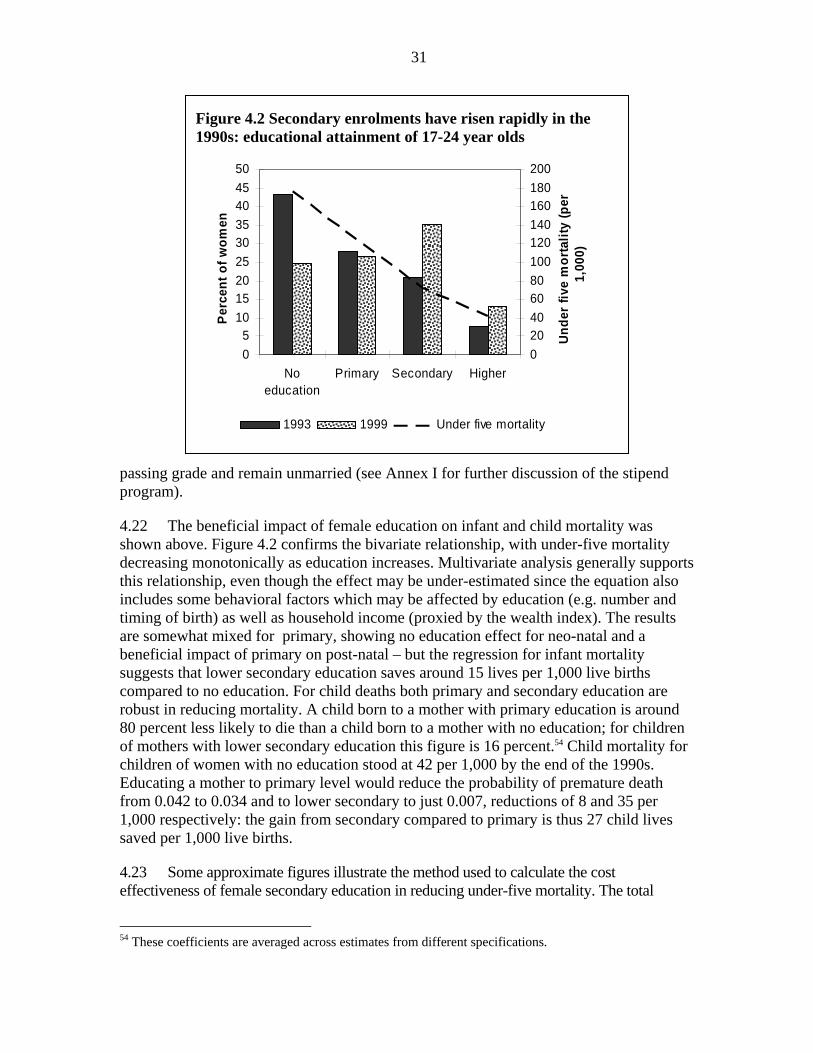
31

passing grade and remain unmarried (see Annex I for further discussion of the stipend program).

4.22 The beneficial impact of female education on infant and child mortality was shown above. Figure 4.2 confirms the bivariate relationship, with under-five mortality decreasing monotonically as education increases. Multivariate analysis generally supports this relationship, even though the effect may be under-estimated since the equation also includes some behavioral factors which may be affected by education (e.g. number and timing of birth) as well as household income (proxied by the wealth index). The results are somewhat mixed for primary, showing no education effect for neo-natal and a beneficial impact of primary on post-natal – but the regression for infant mortality suggests that lower secondary education saves around 15 lives per 1,000 live births compared to no education. For child deaths both primary and secondary education are robust in reducing mortality. A child born to a mother with primary education is around 80 percent less likely to die than a child born to a mother with no education; for children of mothers with lower secondary education this figure is 16 percent.54 Child mortality for children of women with no education stood at 42 per 1,000 by the end of the 1990s. Educating a mother to primary level would reduce the probability of premature death from 0.042 to 0.034 and to lower secondary to just 0.007, reductions of 8 and 35 per 1,000 respectively: the gain from secondary compared to primary is thus 27 child lives saved per 1,000 live births.

4.23 Some approximate figures illustrate the method used to calculate the cost effectiveness of female secondary education in reducing under-five mortality. The total

54 These coefficients are averaged across estimates from different specifications.

Figure 4.2 Secondary enrolments have risen rapidly in the 1990s: educational attainment of 17-24 year olds

05

101520253035404550

Noeducation

Primary Secondary Higher

Perc

ent o

f wom

en

020406080100120140160180200

Unde

r fiv

e m

orta

lity

(per

1,

000)

1993 1999 Under five mortality

32

fertility rate is around 3.3, so that 300 women will, over their lifetimes, give birth to 1,000 children. If these 300 women receive secondary education (rather than primary) then the number of child deaths averted is around 25 (using a conservative estimate based on child deaths only). The stipend cost per girl for the five years of secondary, including administrative costs, is US$90. So the cost of getting the 300 girls to school is US$27,000 (=300x90). The cost per death averted is thus US$1,080 (= 27,000/25). This figure is an under-estimate since infant deaths have been excluded from the calculation, and various indirect behavioral channels are not allowed for. But it is also an over-estimate for the reasons explained in the next paragraph.

4.24 The above calculation assumes that the presence of the program is the reason the girl goes to school. In fact, all rural girls receive the stipend, whether they would have gone to school in the absence of the stipend or not. Determining the marginal impact of the stipend on girls’ enrolment is not that straightforward. Best estimates suggest that of every 10 girls receiving the stipend, two of those would not have gone to school in the absence of the stipend (see Annex I). This raises the cost per death averted by a factor of five to US$5,400.55 While, perhaps unsurprisingly, more expensive than the cost of direct health interventions discussed above, this figure is not high by international standards.

4.25 From 1993-99 an additional 1.4 million girls have attended secondary school, of which 1 million are from rural areas. Over this period, the World Bank provided 0.8 million stipend years which, assuming it was paid to each girl for 4 years, means that 0.2 million additional girls were paid to go to school. These 0.2 million girls will go on to have 660,000 children. Since 25 deaths are averted per 1,000 live births, then 16,500 under-five deaths will be averted by this increased enrolment. As above, it is assumed that the whole enrolment increase is on account of stipends. Adjusting for the likely marginal impact of the program on enrolments reduces the number of deaths averted by the World Bank’s support of the stipend program to 3,300 (i.e., just over one percent of the actual number of under-five deaths each year).

Rural Electrification and Access to Media

4.26 Electrification can affect health outcomes through several channels: (1) income effects, (2) quality of health care, notably the cold chain,56 (3) sanitary environment, including boiled water, and (4) access to media and thus health messages. There is evidence of the importance of each of these effects in the results, partly showing up by a direct effect from the significance of the electrification variable in multivariate analysis.

4.27 A study of the impact of rural electrification conducted for USAID found electrification to cause an increase in income of 15 percent,57 which translates into an 55. This calculation omits the supply-side costs associated with higher enrolments.

56. The cold chain is a system of conservation and distribution of vaccines to maintain them in cold temperatures between 32 and 46.4 degrees Fahrenheit, which id necessary to guarantee their effectiveness.

57. The study found that income in households with electricity was 65 percent higher than that in households of non-electrified villages, and 126 percent higher than households without electricity in electrified villages. Rather than tackle the endogeneity problem econometrically, the study breaks down

33

approximately 11 percent increase in the wealth index used to measure economic well-being in DHS data.58 Given the regression coefficients, electrification-induced income effects have reduced infant mortality by around 5 per 1,000 and for children at around 10 per 1,000. Assigning the whole ‘TV effect’ adds another 8 per thousand, and direct effects another 2 per thousand. Electrification thus reduces the probability of under-five death by 0.025 (25 per thousand). During the 1990s a household connection cost US$500,59 so that connecting 1,000 households cost US$0.5 million. Connecting these 1,000 households will avert 25 deaths, at a cost of US$20,000 each.60 As the program rolls out connections become more expensive, currently reaching around US$1,000 per household, bringing the cost per life saved to US$40,000. Rural electrification is having a measurable impact on child health outcomes. Since there are many other benefits to electrification than reduced mortality, it is unsurprising that the cost per life saved is high relative to that of other interventions.

4.28 Access to media variables – particularly TV and radio – are significant in the outcome regressions for mortality (as well as those for fertility and nutrition). These results provide evidence of the importance and effectiveness of IEC campaigns. Given the diverse nature of these campaigns (see Chapter 2 on the different ministries involved), and different channels through which households access information, it is not possible to quantify their impact and cost effectiveness.

Fertility Reduction

4.29 The cross-country evidence presented at the start of this chapter feeds directly into a debate as to the causes of fertility decline in Bangladesh. Some have claimed that the usual socio-economic factors explaining lower fertility have been absent and that the

income by source to identify those which may be attributed to electrification. On this basis it is concluded that 16.5 percent of the income of electrified households is attributable to electrification (Barkat et al., 2002).

58. Assuming a savings propensity of 0.1 and using the wealth-expenditure elasticity of 0.8 estimated using HIES data (Annex C).

59. The figures of US$500 and US$1,000 per connection were provided by the Task Manager for the Bank’s rural electrification projects. Cost-benefit calculations in the ICR for RE III present cost figures for four new rural electricity cooperatives, giving a discounted cost of Tk 1,686 million cost for 80,210 new residential connections. These figures give a cost of US$470 per residential connection during the 1990s (see Annex I).

60. The number of deaths averted in a household depends on household composition. If all children are already over 5 no deaths are averted, whereas if the mother is just entering her childbearing years then, on average, just over 3 children will be born who are less exposed to risk of premature mortality on account of electrification. An analysis of household structure suggests that on average 1.2 children per household will benefit from the reduced risk due to electrification. Since all figures are indicative of broad orders of magnitude a figure of one child per household is used in the cost effectiveness calculations. However, unlike immunization, which benefits just that child (possibly others through the herd immunization effect discussed above), and schooling, which benefits the children of a single woman, electrification will benefit subsequent generations, so that the cost calculations have an upward bias from this factor. But in comparing with the female schooling calculations they have an over-estimate since the electrification figures include the income effect, which was excluded for schooling.

34

country’s internationally renowned family planning program explains the success in fertility reduction. Others argue that there has been progress – notably reduced poverty and a measure of women’s empowerment – which can explain lower fertility. The evidence presented above shows that both explanations have played a part. Socio-economic changes, including the usual demographic transition effect of mortality reductions driving down fertility, do explain some of Bangladesh’s fertility reduction in recent decades. But not all of it. There is a substantial residual, which is most plausibly explained by the presence of a substantial and successful family planning program.

4.30 Why can the unexplained fertility reduction most plausibly be attributed to the family planning? Evidence to support this argument comes from a number of ways in which Bangladesh is exceptional. First, Figure 4.1(b) already showed the large reduction in fertility, greatly in excess of what would have been expected from the country’s income growth over this period. Second, Figure 3.4 showed that contraceptive knowledge was almost universal in Bangladesh by the early 1980s. Bangladesh is an outlier in this respect, meaning that contraceptive knowledge is much higher than expected for a country of Bangladesh’s income and female education levels. Furthermore, as discussed below, Bangladesh is also an exception in the low level of its fertility given the low age at which women get married. These discrepancies are best explained by the presence of the family planning program. Finally, multivariate analysis confirms the links between family planning acceptance and fertility in Bangladesh (Annex F). Less directly, the analysis shows the importance of access to media in lowering family size, indicating the contribution of IEC campaigns to spreading awareness of small family size and contraceptive knowledge.

4.31 The argument as to the impact of the family planning program in the past matters for the current day since the claimed fertility plateau in the 1990s has cast new doubts on the program’s effectiveness. However, it was shown in the last chapter, that fertility decline did indeed continue throughout the 1990s, with contraceptive usage continuing to grow. There are legitimate concerns among policymakers about contraceptive discontinuation, but it would be mistaken to feel that the program has stalled.

4.32 Nonetheless, fertility decline has slowed, so it is legitimate to ask how momentum may be maintained. The government’s new HNP Strategic Investment Plan highlights the role of increasing the age at marriage as a means of reducing fertility, and several programs, including the counseling provided under the World Bank supported Bangladesh Integrated Nutrition Project (BINP), promote getting married later. It is a condition of the female secondary school stipend program that recipients remain unmarried. It is true that the age at marriage in Bangladesh is low, with half of all women marrying by age 14. It is also true that there is a well-established international pattern whereby increasing the age at marriage drives down fertility. But this pattern should not be expected to be observed in Bangladesh for two reasons: (1) raising the age at marriage of girls aged 13 or less has no effect on the age at which they have their first child (so as the age at marriage has risen the gap from marriage to first birth has fallen, see Annex F), and (2) if a woman plans to have only 3-4 children, as the majority of Bangladeshi women do, then this can be accomplished whether child bearing begins at 15 or 20. The effect of expanding education is muted since Bangladesh has already attained levels of fertility comparable to those in countries with higher levels of education. Hence raising the age at marriage, while desirable for both

35

maternal and child health (children born to young mothers have a greater chance of premature death), 61will have little impact on fertility. On the other hand, there remain a substantial proportion of high fertility households. – reducing fertility amongst these would make an important contribution to continued fertility decline. One means of doing this would be to attempt to restore the use of permanent contraception to its previous level – long-term methods accounted for 30 percent of contraceptive use in 1991, but only 12 percent by 2004.62 Higher fertility women are less likely to be utilizing health services, so that the case for home visits should be reconsidered as a part of the wider strategy for fertility reduction. In addition, though it is difficult to suggest appropriate policy responses, attempts can be made to tackle son preference which creates a barrier to fertility decline.

Nutrition

4.33 In recent years the main focus for improving nutritional outcomes has been through BINP, which is the subject of the next chapter. However, BINP has had a limited geographical focus, while, as shown in Chapter 3, nutritional status has been improving across the country. DHS collected anthropometric data in 1996 and 1999, which thus allows some analysis of the factors behind this improvement. OED analysis shows that:

• Wealth is a significant determinant of a child’s nutritional status, and the increase in the wealth index between the two surveys accounts for close to 10 percent of the observed reduction in stunting.

• Mother’s education to secondary level improves child nutrition – whereas children of mothers with primary education alone have no nutritional advantage over those whose mothers have no education. The expansion of secondary education accounts for about 6 percent of the observed fall in stunting. These nutritional gains can be added to the beneficial impact of FSSAP.

• A household having electricity reduces the probability of stunting; service expansion accounts for about 4 percent of the fall in stunting in the late 1990s.

• Children of lower birth order have better nutritional status, capturing the advantage of smaller family size in limiting resource competition among young children. The reduction in mean birth order, as a result of falling fertility, accounted for about 6 percent of the improvement in nutritional status.

• The regression results leave a fair amount of the reduction in stunting unexplained. Possible reasons for this decline are picked up in the next chapter which discusses the Bangladesh Integrated Nutrition Project in greater depth.

61. The effect of delayed marriage in reducing mortality introduces a ‘second order effect’ channel through which delaying marriage will indeed reduce fertility. 62 Of course this decline partly represents the fact that women subject to permanent methods by questionable, semi-coercive means used in the early years of the program are leaving the group of women covered by the DHS.

36

5. A Closer Look at Nutrition: The Bangladesh Integrated Nutrition Project

The Community-Based Nutrition Component of BINP was to improve nutritional status through nutritional counseling and supplementary feeding for malnourished children and pregnant women. Both counseling and feeding suffered from problems of inappropriate targeting strategies and a failure to reach intended groups. While counseling has changed women’s knowledge it has had less of an impact on behavior. There is a knowledge-practice gap, which is explained by resource constraints, including lack of time, faced by women which prevent them from putting the advice into practice. The impact of the project on anthropometric outcomes has not been large, so that the approach does not appear to be a cost effective means of tackling poor nutrition.

5.1 While rapid strides were being made in reducing mortality and fertility in the 1980s, malnutrition showed no improvement, affecting close to seventy percent of all children under-five. In order to address this remaining problem the government undertook a pilot nutrition intervention supported by the World Bank, the Bangladesh Integrated Nutrition Project (BINP), which was to initiate a national program whose ultimate goal was to reduce malnutrition to the extent that it ceased to be a public health problem. More specific targets – such as the reduction of severe malnutrition by 40 percent and moderate malnutrition by 25 percent in the project areas – were also set. The project is now being scaled-up to the national level. This chapter takes a look at the evidence regarding the effectiveness of the BINP’s main component, the Community Based Nutrition Component (CNBC).

5.2 BINP, and notably the CNBC, has been the subject of several studies: the independent evaluation of BINP for the project (Karim et al., 2003), a study by Save the Children (2003), an evaluation commissioned by the government’s evaluation department (Implementation, Monitoring and Evaluation Department, IMED; Haider et al, 2004) and two PhD theses from the University of Cambridge. For this study OED has obtained the BINP evaluation and Save the Children data sets.63 The analysis is extended from that contained in the above-mentioned reports through the application of a theory-based evaluation framework, and improving on the quality of the control for the BINP evaluation data set by using a nationally representative sample survey to construct a new control using propensity score matching.64

63. Thanks are due to the staff the World Bank nutrition hub for facilitating access to the BINP evaluation data set, to Save the Children for providing their data, and the staff of Helen Keller International Dhaka for providing the Nutritional Surveillance Project data.

64. Theory-based evaluation is propounded in Weiss (1998); see Carvalho and White (2004) for an application to development projects.

37

Overview of the Project

5.3 BINP had three components: (1) National Nutrition Activities (US$20.6 million), including institutional development, IEC and monitoring and evaluation (M&E); (2) Community-Based Nutrition (US$39.1 million); and (3) Inter-sectoral Nutrition Program Development (US$7.6 million), supporting schemes such as home gardening and poultry rearing which would have beneficial effects for nutrition.

5.4 CNBC was the main component, and the one which is focused on here. In each project thana a number of Community Nutrition Promoters (CNPs) were recruited, these being local women with children of their own and having achieved at least an eighth grade education. The CNPs implemented activities at the community level: monthly growth monitoring for children under 24 months old, supplementary feeding for malnourished children and pregnant women, and nutritional counseling in a variety of settings. The CNPs were overseen by a Community Nutrition Officer, and supervisors at the thana level who were staff of the implementing NGO.65

The Theory Underlying the CNBC

5.5 The key assumption behind CNBC is that “bad practices” are responsible for malnutrition in Bangladesh. This point of view was strongly argued in the BINP appraisal document: “behaviors related to feeding of young children have at least as much (if not more) to do with the serious problem of malnutrition in Bangladesh as poverty and the resultant household food insecurity do” (BINP SAR: para 1.13, p.4; World Bank, 1995). Therefore changing bad practice to good will bring about nutritional improvements. There are a number of steps in the causal chain behind this approach:

• The right people (those making decisions regarding under-nourished children) are targeted with nutritional messages

• These people participate in project activities, and so are exposed to these messages

• Exposure leads to acquisition of the desired knowledge • Acquisition of the knowledge leads to its adoption (i.e., a change in practice) • The new practices make a substantial impact on nutritional outcomes

5.6 A feeding program for malnourished children and pregnant women was implemented alongside growth monitoring. For this program to work:

• The target groups have to enroll in the program • The criteria are correctly applied in selecting those to receive supplementary

feeding • Those selected for supplementary feeding attend sessions to receive the food. • There is no leakage (e.g., selling of food supplements), or substitution (reducing

other food intake)

65. In some thanas BINP was implemented by GoB, so that this last level of supervision was missing.

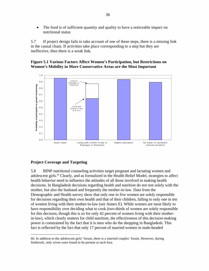
38

• The food is of sufficient quantity and quality to have a noticeable impact on nutritional status

5.7 If project design fails to take account of one of these steps, there is a missing link in the causal chain. If activities take place corresponding to a step but they are ineffective, then there is a weak link.

Figure 5.1 Various Factors Affect Women’s Participation, but Restrictions on Women’s Mobility in More Conservative Areas are the Most Important

Project Coverage and Targeting

5.8 BINP nutritional counseling activities target pregnant and lactating women and adolescent girls.66 Clearly, and as formalized in the Health Belief Model, strategies to affect health behavior need to influence the attitudes of all those involved in making health decisions. In Bangladesh decisions regarding health and nutrition do not rest solely with the mother, but also the husband and frequently the mother-in-law. Data from the Demographic and Health survey show that only one in five women are solely responsible for decisions regarding their own health and that of their children, falling to only one in ten of women living with their mother-in-law (see Annex E). While women are most likely to have responsibility over deciding what to cook (two-thirds of women are solely responsible for this decision, though this is so for only 42 percent of women living with their mother-in-law), which clearly matters for child nutrition, the effectiveness of this decision-making power is constrained by the fact that it is men who do the shopping in Bangladesh. This fact is reflected by the fact that only 17 percent of married women in male-headed 66. In addition to the adolescent girls’ forum, there is a married couples’ forum. However, during fieldwork, only wives were found to be present at such fora.

0 .0

0 .1

0 .2

0 .3

0 .4

0 .5

0 .6

0 .7

0 .8

0 .9

1 .0

B a se va lu e L iv ing w ith m o th e r-in -la w inR a jn a ga r o r S ha h ra s ti

H igh e r e d uca tion N o w a te r o r sa n ita tio n(re m o te lo ca tio n )

Prob

abili

ty o

f par

ticip

atio

n in

gro

wth

mon

itorin

ng

L iv in g in R a jna g a r o r

S ha h ra s ti

L iv ing w ith m o th e r- in - la w

in R o r S

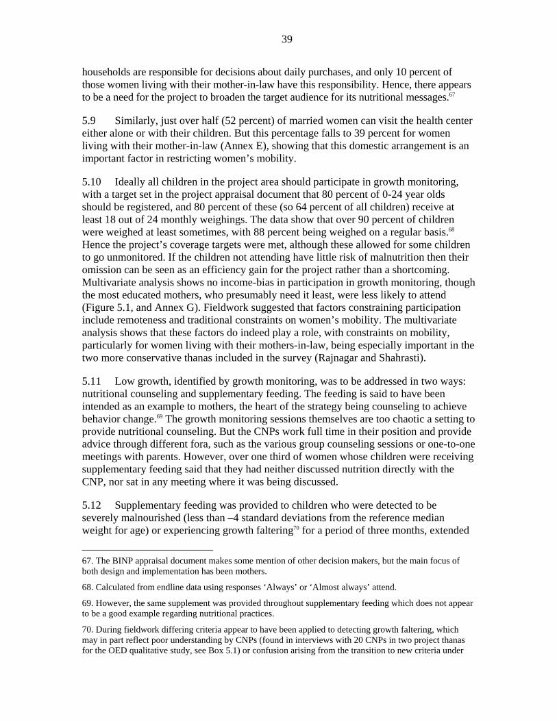
39

households are responsible for decisions about daily purchases, and only 10 percent of those women living with their mother-in-law have this responsibility. Hence, there appears to be a need for the project to broaden the target audience for its nutritional messages.67

5.9 Similarly, just over half (52 percent) of married women can visit the health center either alone or with their children. But this percentage falls to 39 percent for women living with their mother-in-law (Annex E), showing that this domestic arrangement is an important factor in restricting women’s mobility.

5.10 Ideally all children in the project area should participate in growth monitoring, with a target set in the project appraisal document that 80 percent of 0-24 year olds should be registered, and 80 percent of these (so 64 percent of all children) receive at least 18 out of 24 monthly weighings. The data show that over 90 percent of children were weighed at least sometimes, with 88 percent being weighed on a regular basis.68 Hence the project’s coverage targets were met, although these allowed for some children to go unmonitored. If the children not attending have little risk of malnutrition then their omission can be seen as an efficiency gain for the project rather than a shortcoming. Multivariate analysis shows no income-bias in participation in growth monitoring, though the most educated mothers, who presumably need it least, were less likely to attend (Figure 5.1, and Annex G). Fieldwork suggested that factors constraining participation include remoteness and traditional constraints on women’s mobility. The multivariate analysis shows that these factors do indeed play a role, with constraints on mobility, particularly for women living with their mothers-in-law, being especially important in the two more conservative thanas included in the survey (Rajnagar and Shahrasti).

5.11 Low growth, identified by growth monitoring, was to be addressed in two ways: nutritional counseling and supplementary feeding. The feeding is said to have been intended as an example to mothers, the heart of the strategy being counseling to achieve behavior change.69 The growth monitoring sessions themselves are too chaotic a setting to provide nutritional counseling. But the CNPs work full time in their position and provide advice through different fora, such as the various group counseling sessions or one-to-one meetings with parents. However, over one third of women whose children were receiving supplementary feeding said that they had neither discussed nutrition directly with the CNP, nor sat in any meeting where it was being discussed.

5.12 Supplementary feeding was provided to children who were detected to be severely malnourished (less than –4 standard deviations from the reference median weight for age) or experiencing growth faltering70 for a period of three months, extended

67. The BINP appraisal document makes some mention of other decision makers, but the main focus of both design and implementation has been mothers.

68. Calculated from endline data using responses ‘Always’ or ‘Almost always’ attend.

69. However, the same supplement was provided throughout supplementary feeding which does not appear to be a good example regarding nutritional practices.

70. During fieldwork differing criteria appear to have been applied to detecting growth faltering, which may in part reflect poor understanding by CNPs (found in interviews with 20 CNPs in two project thanas for the OED qualitative study, see Box 5.1) or confusion arising from the transition to new criteria under

40

for a further month if they did not show the required weight gain. Analysis of register and field data from the Cambridge studies showed a reasonably low Type II error:71 only 16 percent of children receiving food supplementation should not have been doing so.72 However, of those enrolled, only one-quarter (26 percent) received supplementation for the recommended three months, the majority dropping out sooner. And Type I error was very high: over two-thirds (69.8 percent) of eligible children were not being fed.73

5.13 While an acceptably low percentage of ineligible children were being fed, the criteria themselves are open to question. Growth faltering is quite normal, so enrolling growth faltering children regardless of their nutritional level will mean enrolling perfectly well-nourished children: one study found that 37 percent of a group of US children from well off backgrounds would qualify for supplementary feeding under the criteria used in the Tamil Nadu Integrated Nutrition Project in India (Martorell and Shekar, 1992). The Save the Children register data show that over 40 percent of those enrolled in the feeding program were not malnourished (i.e., the children were above –2 SDs WAZ).

5.14 Turning to monitoring of pregnancy weight gain, close to three-quarters of pregnant women attended weighing sessions, and just under half received supplementary feeding, with both these percentages being a bit lower at endline than the baseline. There is no pattern between attendance at weighing sessions and the mother’s nutritional status, which is to be expected. Supplementary food was meant to be received by women not having normal Body Mass Index. However, by the endline about 60 percent of eligible women were not receiving the supplement. On the other hand, 40 percent of those who were receiving the supplement were not eligible.74

5.15 For both children and mothers there is evidence of both leakage and substitution of the food supplement. For example, 32 percent of women said they had shared their food supplement with someone else. Many of those who were not sharing said they did not eat more during pregnancy than usual, indicating that the BINP provided food was

NNP. For normal children, the official criteria appear to have been less than 600 g. gain in 2 months for those aged 6-12 months and 300 g. in 2 months for those aged 12-24 months. For children with WAZ < - 2 SDs these figures apply to a 3 month period.

71. Type I error is the proportion of the target group not receiving the benefit, and Type II error the proportion of those receiving the benefit who are not eligible to do so.

72. This analysis requires information on pre-feeding nutritional status, which is not available in the BINP evaluation and Save the Children datasets. Save the Children also collected register data, but only for children in the feeding program, so Type I error cannot be calculated from these data. The Type II error calculated from the Save the Children register data is 15.4 percent, almost identical to that found in the Cambridge studies.

73. A number of factors probably lay behind poor targeting, one of which is certainly the difficulty CNPs have in interpreting the quite complex eligibility criteria. Impressions gathered in fieldwork suggest this to be a factor, though there are no numbers to present. The Save the Children data show that the majority of mothers do not understand the growth charts.

74. Data are not available on pre-pregnancy weight. The BMI used here is calculated from data for women not more than six months pregnant, so there will have been some pregnancy weight gain, thus providing an upward bias to the estimate of Type II error – but a downward bias on the estimate of Type I error.

41

substituting for other foodstuffs. This was possible, since many women and children, contrary to project design, consumed the food at home.

5.16 In summary, enrolment in growth monitoring sessions has been at a reasonable level for both children and pregnant women. However, attendance at these sessions has not provided opportunities for nutritional counseling for a sizeable minority of women. There have been problems in the targeting of feeding programs, especially the exclusion of eligible participants for both children and pregnant women. In the case of pregnant women, a considerable number of feeding beneficiaries are in fact ineligible. Such Type II error is less of a problem for child feeding, though the entry criteria themselves appear inappropriate, and only a minority of enrolled children complete the full three months of feeding.

Acquiring Knowledge

5.17 The central thrust of project design was to change nutritional behavior of child caretakers. There are a number of nutritional practices considered adverse to child nutrition. Some are simple differences in habit, such as cutting vegetables before washing them rather than vice versa, which is nutritionally disadvantageous. Others, such as eating less during pregnancy (“eating down”), result from different perceptions of health risks and benefits (mothers perceive the benefit of a lower-risk delivery of a smaller child, discounting the risks to low birth weight children).75 And others stem from traditional beliefs which appear to have no plausible health-related rationale, such as avoiding meat, fish and eggs during pregnancy.

5.18 Data from both Save the Children and the BINP evaluation show that knowledge with respect to good nutritional practices is indeed higher in project areas than in the control. For example 63 percent of women in project areas say that the baby should be fed the colostrums (the first milk), compared to only 52 percent in the control area: a difference of 11 percent. The BINP dataset allows examination of the double difference for two variables, for both of which there has been an increase in knowledge in the project area but not in the control. At the baseline, a slightly higher percentage of women in the control thought it advisable to eat more during pregnancy than was the case in the project area. This proportion had not changed in the control areas, whereas in the project area it rose by 28 percent (which is therefore the double difference effect, since there was no change in the control).

5.19 Of course other factors may be affecting knowledge, such as superior education in the project area. Multivariate regression analysis was used to control for these factors (Annex G). The probability of a mother knowing a specific practice was modeled as a function of mother’s age, education, education of the household head, whether the woman was a group member and participation in project activities. In the Save the Children data variables were included in the analysis of whether a woman simply lived in 75. Eating down was recommended medical practice in European countries for this reason until the 1940s. There is not unanimity regarding the ‘accepted wisdom’, with a recent Australian study finding that women delivering children with a higher birth weight are more likely to require a Caesarian section.

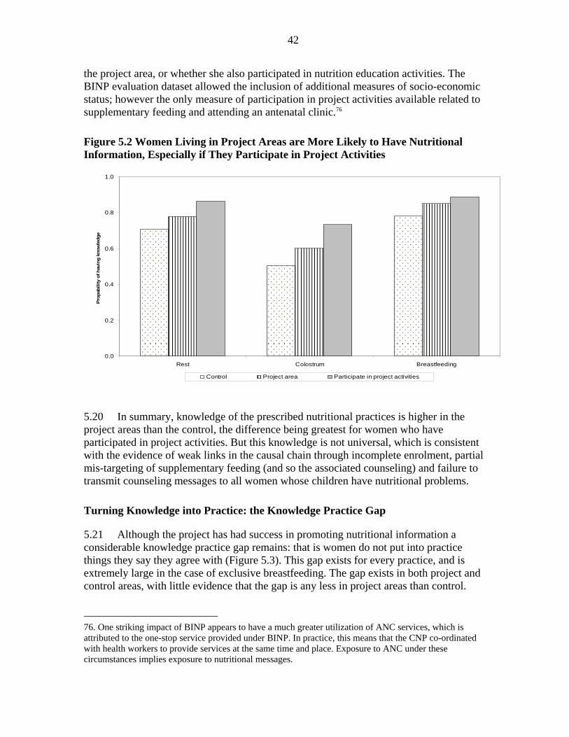
42

the project area, or whether she also participated in nutrition education activities. The BINP evaluation dataset allowed the inclusion of additional measures of socio-economic status; however the only measure of participation in project activities available related to supplementary feeding and attending an antenatal clinic.76

Figure 5.2 Women Living in Project Areas are More Likely to Have Nutritional Information, Especially if They Participate in Project Activities

5.20 In summary, knowledge of the prescribed nutritional practices is higher in the project areas than the control, the difference being greatest for women who have participated in project activities. But this knowledge is not universal, which is consistent with the evidence of weak links in the causal chain through incomplete enrolment, partial mis-targeting of supplementary feeding (and so the associated counseling) and failure to transmit counseling messages to all women whose children have nutritional problems.

Turning Knowledge into Practice: the Knowledge Practice Gap

5.21 Although the project has had success in promoting nutritional information a considerable knowledge practice gap remains: that is women do not put into practice things they say they agree with (Figure 5.3). This gap exists for every practice, and is extremely large in the case of exclusive breastfeeding. The gap exists in both project and control areas, with little evidence that the gap is any less in project areas than control.

76. One striking impact of BINP appears to have a much greater utilization of ANC services, which is attributed to the one-stop service provided under BINP. In practice, this means that the CNP co-ordinated with health workers to provide services at the same time and place. Exposure to ANC under these circumstances implies exposure to nutritional messages.

0.0

0.2

0.4

0.6

0.8

1.0

Rest Colostrum Breastfeeding

Prop

abili

ty o

f hav

ing

know

ledg

e

Control Project area Participate in project activities

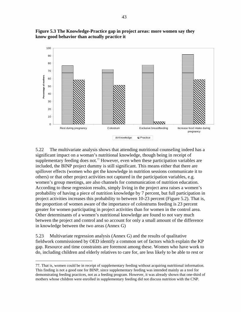
43

Figure 5.3 The Knowledge-Practice gap in project areas: more women say they know good behavior than actually practice it

5.22 The multivariate analysis shows that attending nutritional counseling indeed has a significant impact on a woman’s nutritional knowledge, though being in receipt of supplementary feeding does not.77 However, even when these participation variables are included, the BINP project dummy is still significant. This means either that there are spillover effects (women who get the knowledge in nutrition sessions communicate it to others) or that other project activities not captured in the participation variables, e.g. women’s group meetings, are also channels for communication of nutrition education. According to these regression results, simply living in the project area raises a women’s probability of having a piece of nutrition knowledge by 7 percent, but full participation in project activities increases this probability to between 10-23 percent (Figure 5.2). That is, the proportion of women aware of the importance of colostrums feeding is 23 percent greater for women participating in project activities than for women in the control area. Other determinants of a women’s nutritional knowledge are found to not vary much between the project and control and so account for only a small amount of the difference in knowledge between the two areas (Annex G)

5.23 Multivariate regression analysis (Annex G) and the results of qualitative fieldwork commissioned by OED identify a common set of factors which explain the KP gap. Resource and time constraints are foremost among these. Women who have work to do, including children and elderly relatives to care for, are less likely to be able to rest or

77. That is, women could be in receipt of supplementary feeding without acquiring nutritional information. This finding is not a good one for BINP, since supplementary feeding was intended mainly as a tool for demonstrating feeding practices, not as a feeding program. However, it was already shown that one-third of mothers whose children were enrolled in supplementary feeding did not discuss nutrition with the CNP.

0

10

20

30

40

50

60

70

80

90

100

Rest during pregnancy Colostrum Exclusive breastfeeding Increase food intake duringpregnancy

Per

cent

age

of m

othe

rs

Knowledge Practice

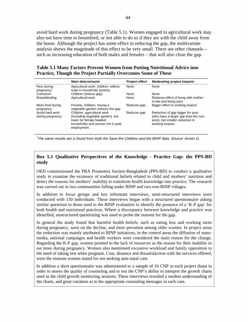
44

avoid hard work during pregnancy (Table 5.1). Women engaged in agricultural work may also not have time to breastfeed, or not able to do so if they are with the child away from the home. Although the project has some effect in reducing the gap, the multivariate analysis shows the magnitude of this effect to be very small. There are other channels – such as increasing education of both males and females – that will also close the gap.

Table 5.1 Many Factors Prevent Women from Putting Nutritional Advice into Practice, Though the Project Partially Overcomes Some of These Main determinants Project effect Moderating project impacts Rest during pregnancy*

Agricultural work, children, elderly male in household, poverty

None None

Colostrum Children (reduce gap) None None Breastfeeding Agricultural work None Reduces effect of living with mother-

in-law and being poor More food during pregnancy

Poverty, children, having a vegetable garden reduces the gap

Reduces gap Bigger effect in working season

Avoid hard work during pregnancy

Children, agricultural work (including vegetable garden), but lower for female headed households and women not in paid employment

Reduces gap Reduction of gap bigger for poor (who have a larger gap than the non-poor), but smaller reduction in working season.

*The same results are is found from both the Save the Children and the BINP data. Source: Annex G.

Box 5.1 Qualitative Perspectives of the Knowledge - Practice Gap: the PPS-BD study

OED commissioned the PRA Promoters Society-Bangladesh (PPS-BD) to conduct a qualitative study to examine the existence of traditional beliefs related to child and mothers’ nutrition and detect the reasons for mothers’ inability to transform health knowledge into practice. The research was carried out in two communities falling under BINP and two non-BINP villages.

In addition to focus groups and key informant interviews, semi-structured interviews were conducted with 150 individuals. These interviews began with a structured questionnaire asking similar questions to those used in the BINP evaluation to identify the presence of a ‘K-P gap’ for both health and nutritional practices. Where a discrepancy between knowledge and practice was identified, unstructured questioning was used to probe the reasons for the gap.

In general the study found that harmful health beliefs, such as eating less and working more during pregnancy, were on the decline, and more prevalent among older women. In project areas the reduction was mainly attributed to BINP initiatives, in the control areas the diffusion of mass-media, national campaigns and health workers were considered the main reason for the change. Regarding the K-P gap, women pointed to the lack of resources as the reason for their inability to eat more during pregnancy. Women also mentioned excessive workload and family opposition to the need of taking rest when pregnant. Cost, distance and dissatisfaction with the services offered, were the reasons women stated for not seeking ante-natal care.

In addition a short questionnaire was administered to a sample of 10 CNP in each project thana in order to assess the quality of counseling and to test the CNP’s ability to interpret the growth charts used in the child growth monitoring sessions. These interviews revealed a modest understanding of the charts, and great variation as to the appropriate counseling messages in each case.

45

5.24 In summary, the project does increase knowledge about nutritional practices. However, there is a gap between knowledge and practice, and the project does not have an impact in reducing the size of the gap. But since knowledge is more widespread, and the gap the same in project and control areas, then the promoted practices are more widespread in the project area. So, are these practices beneficial to nutritional outcomes?

The Nutritional Impact of BINP Interventions

Child Nutrition

5.25 Existing studies have found somewhat different results with respect to the impact of BINP, though where an impact has been found its magnitude is not that great. This study used the nationally representative Nutritional Surveillance Project data to construct a control group using propensity score matching. These results find a significant project impact from BINP at midline on all three z-scores of just over 0.1. However, at endline the impacts are smaller and most are not significant. This figure means that the project reduced malnutrition in project areas by at most 5 percent – well short of the project target, so the project failed to achieve its central objective.

5.26 It is difficult to construct a suitable control for supplementary feeding. However, the best estimate possible suggests that a child receiving feeding has a weight gain equal to 0.1 WAZ for those under 12 months old, and over 0.4 for those over one year of age. The NSP data show that WAZ falls by about 0.5 WAZ over a three-month period for children under 12 months, and then stabilizes: hence supplementary feeding has a positive impact for children of this age of around 0.6 WAZ. The impact is greater still for children who entered the program more malnourished.

Low Birth Weight

5.27 BINP aimed to increase pregnancy weight gain by both encouraging women to eat more during pregnancy and providing supplementary feeding to malnourished pregnant women. While there was a striking improvement in pregnancy weight gain in project areas, there was an even greater improvement in the control, suggesting that non-project factors played a large role in the observed improvements. Nonetheless, multivariate analysis suggests that there was some project effect, of about 200 gram per month, mainly through the fact that women in project areas were more likely to eat more during pregnancy than those in the control.78 The project-related weight gain is thus not much more than 1 kilogram over six months which, evidence suggests, increases birth weight by only 20 grams. That is, the amount of pregnancy weight gain appears insufficient to have a substantial impact on low birth weight.

78. Participation in supplementary feeding was not found to have a significant impact. This impact may have been muted by leakage and substitution.

46

5.28 This conclusion is supported by direct estimates of project impact on low birth rate, although these suggest a slightly larger impact of about 80 grams, again mainly as a result of the mother not eating down. However, there is a much stronger impact of around 270 grams for children born to women with poor nutritional status, which is reassuring as women of low body-mass index (BMI) need a larger pregnancy weight gain to avoid low birth weight than do women with a higher than average BMI. The project also seems to smooth out the seasonal effects that come from mothers being less well nourished in the lean season, which is most likely a result of supplementary feeding.

Cost-Effectiveness Analysis

5.29 The impact results can be used to calculate the cost to move a child out of malnutrition, the results of which are shown in Table 5.2. The first two rows of the table show the average amount of funds to be invested on a child over a year in order to move the child out of malnutrition, measured by WAZ and HAZ. Based on estimates of the relationship between child malnutrition and mortality, the last row shows the amount of money to be spent in order to save one life. For the BINP project, these figures were obtained using data on project costs, population of project areas, and project effects on malnutrition rates at the midterm and the endline (see Annex G). The rice ration simulation uses the relationship between food intake and physical growth observed in other studies, and simulates the nutritional effects of investing BINP funds on the same areas and population covered by the BINP project in 1998. The unit cost of saving one live and a malnourished child is less under the rice ration simulation, because given the assumption used, this intervention would produce a larger reduction in malnutrition. The cost (using CBNC costs associated with children, i.e. excluding those for pregnant women) per life saved from improved nutritional status is also shown. For comparative purposes the results of a simulation assuming that the project funds were instead used to purchase rice which was given to families with children is also shown,79 which proves to be a more cost effective route to improving child nutrition.

Table 5.2 Cost of Nutrition Improvements and Mortality Reduction (US$)

BINP Rice ration

Midterm (1998) Endline (2003)

Weight-for-age 187 333 110

Height-for-age 241 490 n.a.

Per life saved 2328 4095 2223

Other Sources of Improved Nutritional Outcomes

5.30 Both the OED results and the BINP evaluation find a stronger impact on child nutrition at midterm than endline. Between midterm and endline, pregnancy weight gain 79. The assumptions underlying this calculation are laid out in Annex G. A 25 percent administrative overhead was allowed.

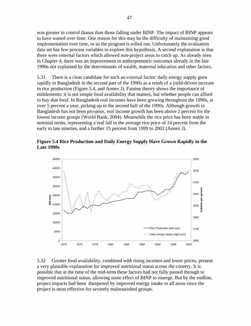
47

0

5000

10000

15000

20000

25000

30000

35000

40000

45000

1970 1974 1978 1982 1986 1990 1994 1998 2002

000

tons

1600

1700

1800

1900

2000

2100

2200

2300

Cal

orie

s pe

r per

son

Rice Production (left axis)

Daily energy supply (right axis)

was greater in control thanas than those falling under BINP. The impact of BINP appears to have waned over time. One reason for this may be the difficulty of maintaining good implementation over time, or as the program is rolled out. Unfortunately the evaluation data set has few process variables to explore this hypothesis. A second explanation is that there were external factors which allowed non-project areas to catch up. As already seen in Chapter 4, there was an improvement in anthropometric outcomes already in the late 1990s not explained by the determinants of wealth, maternal education and other factors.

5.31 There is a clear candidate for such an external factor: daily energy supply grew rapidly in Bangladesh in the second part of the 1990s as a result of a yield-driven increase in rice production (Figure 5.4, and Annex J). Famine theory shows the importance of entitlements: it is not simple food availability that matters, but whether people can afford to buy that food. In Bangladesh real incomes have been growing throughout the 1990s, at over 5 percent a year, picking up in the second half of the 1990s. Although growth in Bangladesh has not been pro-poor, real income growth has been above 2 percent for the lowest income groups (World Bank, 2004). Meanwhile the rice price has been stable in nominal terms, representing a real fall in the average rice price of 14 percent from the early to late nineties, and a further 15 percent from 1999 to 2002 (Annex J).

Figure 5.4 Rice Production and Daily Energy Supply Have Grown Rapidly in the Late 1990s

5.32 Greater food availability, combined with rising incomes and lower prices, present a very plausible explanation for improved nutritional status across the country. It is possible that at the time of the mid-term these factors had not fully passed through to improved nutritional status, allowing some effect of BINP to emerge. But by the endline, project impacts had been dampened by improved energy intake in all areas since the project is most effective for severely malnourished groups.

48

Testing the Theory in Practice - How Well Did the Causal Chain Operate?

5.33 BINP succeeded in achieving high levels of participation in its activities in project areas, enrolled large numbers in supplementary feeding, brought about significant increases in nutritional knowledge and, to a lesser extent, associated changes in practice. However, nutritional outcomes in terms of low birth weight have been disappointing. While child nutrition, especially for children participating in supplementary feeding, appears to have been better, the overall difference in performance compared to the control is not great.

5.34 The longer the causal chain, the more likely it is that final outcomes will not be realized on account of missing or weak links in the chain, and since there are more opportunities for external factors to undermine the ‘logical flow from inputs to outcomes’. There were two missing links in the BINP chain: the first was the relative neglect of some key decision makers regarding nutritional choices (men and mothers-in-law), and the second the focus on pregnancy weight gain rather than pre-pregnancy nutritional status. Participation levels of the target audience were high, but many women escaped exposure to nutritional messages, and there was a high Type I error in the feeding programs (see Table 5.3). A substantial knowledge practice gap persisted, so many women did not put the advice they received into practice, especially if they were resource or time constrained. Those receiving supplementary feeding, often shared it with others or substituted it for their regular foodstuffs. This list of weak links in the chain explain why project impact was muted by the time final outcomes are considered. While attention can be paid to each of these weak links, the BINP experience does demonstrate the difficulty of implementing complex designs.

5.35 Given that the nutritional gains from the project are small it does not appear to be a particularly cost effective intervention. The cost for reducing malnutrition rates appear high, apparently more costly than simply buying food and giving it away, even allowing for a 25 percent administrative cost to do so. The efficacy and efficiency of the program must be improved if it is to justify its continued existence.

49

Table 5.3 Links in the Causal Chain

Assumption Children Mothers Attend growth monitoring sessions

Over 90 percent of children attend GM sessions

Over 70 percent participate in monitoring pregnancy weight gain

Targeting criteria correctly applied; participants stay in program to receive food

Nearly two-thirds of eligible children not fed (reasons: don’t attend GM in first place, wrong application of targeting criteria, drop out of feeding)

60 percent of eligible women not receiving supplementary feeding

Acquire knowledge and put it into practice

One-third of mothers of children receiving supplementary feeding do not receive nutritional counseling. There is a knowledge practice gap (see mothers).

There is a knowledge practice gap, driven by material resource or time constraints.

No leakage or substitution One quarter of children fed at home, increasing possibility of both leakage and substitution.

One-third admit sharing food, and there is substitution for those who do not. At most 40 percent of eligible women receive full supplementation.

Feeding and nutritional advice have an impact on nutritional status

Supplementary feeding has a positive impact on child nutritional status, especially for the most malnourished children. There is only weak evidence of any impact from nutritional counseling.

Pregnancy weight gain is too little to have a notable impact on low birth weight, except for most malnourished mothers. Moreover, mother’s pre-pregnancy nutritional status is more important than pregnancy weight gain. Consequently, birth weight gains are slight, though greater for children of severely malnourished mothers. Eating more during pregnancy is the main channel for both pregnancy weight gain and higher birth weight.

50

6. Lessons Learned

Externally supported interventions have had a notable impact on MCH-related outcomes in Bangladesh. Immunization has proved particularly cost effective, and has saved the lives of up to two million children under the age of five

6.1 Immunization has prevented up to 2 million children from dying prematurely since the launch of the Expanded Program of Immunization, at a cost of less than US$200 per death averted. Among the benefits which may be attributed to World Bank support are 200,000 lives saved through immunization and 3,300 saved through support for the Female Secondary School Assistance Project.

World Bank support to sectors outside of health has contributed to better child health outcomes

6.2 Interventions in different sectors affect maternal and child health. The World Bank has supported both female secondary schooling and rural electrification, both of which have reduced under-five mortality.

Small amounts of money save lives…though the amount varies significantly by intervention

6.3 Immunization is the most cost-effective means of saving lives. But even interventions outside the health sector can avert deaths at a relatively low cost (Table 6.1). These reductions in mortality are on top of the other benefits from these interventions, such as higher income from rural electrification, and lower fertility from female education.

Table 6.1 Cost-effectiveness of Different Interventions in Reducing Under-Five Mortality (US$ per death averted) Lower estimate Upper estimate Immunization 100 300 Training TBAs 220 800 Female secondary school stipend

1,080 5,400

BINP 2,300 4,100 Rural electrification 20,000 40,000

Source: OED analysis.

Although interventions from many sectors affect maternal and child health outcomes, this fact need not imply that multi-sectoral interventions are always needed

6.3 This study has shown that interventions in one sector affect outcomes in other sectors. But they were not multi-sectoral interventions. The female stipend program is implemented under the auspices of the Ministry of Education, and electrification by Rural Electrification Boards. There was no need for the Ministry of Health and Family Welfare to

51

implement its own education stipend programs or construct electricity generators – nor even for them to be consulted on the implementation of these programs by the responsible line ministries – for these inter-sectoral impacts to be felt. It is important that the presence of inter-sectoral impacts not be confused with the need for multi-sectoral interventions or over-centralization of sectoral activities.

World Bank support for training traditional birth attendants has reduced neonatal mortality…but this program has now been abandoned following the international trend toward support for skilled birth attendants

6.4 Analysis of DHS data shows that TBA training in the 1990s reduced infant mortality. However, support to training TBAs stopped as the international Safe Motherhood Initiative chose to emphasize instead the role of skilled birth attendants. While training TBAs has had limited impact on maternal mortality in Bangladesh, as a result of weak emergency obstetric care, TBAs continue to attend over half of all births. Given this situation, one that is likely to take time to change, it is unwise to make such a wholesale policy turnaround. In Bangladesh the Bank followed this trend and dropped the training of TBAs from its projects, even though there was no local evidence to support such a decision.

Programs should be based on local evidence, rather than general conventional wisdom

6.5 The abandonment of training TBAs is an example of the general finding of the importance of taking context into account in program design.

6.6 A second example is the effect that raising the age at marriage can have on fertility. There is a well-established relationship by which an increase in the age at marriage drives fertility reduction. However, there is a simple argument why this effect will be considerably less in Bangladesh than elsewhere: that is, fertility has already been reduced to levels compatible with a far greater age at marriage than currently observed. Based on current international norms, the average age at marriage could rise by over two years and Bangladesh would still have lower fertility than other countries with similar marital ages. While increasing the age at marriage has benefits for child health, its impact on fertility is likely to be limited. Strategies to reduce fertility would better target activities toward the pockets of high fertility.

Gender issues are central to health strategies in Bangladesh…more attention is needed to redressing gender biases to maintain momentum in mortality decline and fertility reduction. But traditional attitudes are not the absolute constraint on service provision which is sometimes suggested.

6.7 The study finds strong evidence of son preference which both acts as a barrier to fertility reduction and creates excess mortality among girls. This problem is most severe in the more conservative parts of the country. Tackling gender bias should be a central aspect of health sector strategies.

52

6.8 It is often argued that traditional attitudes toward women in Bangladesh (purdah) act as a constraint on women’s access to health services. There is some evidence that this is the case, which underlines the importance of reaching all decision makers with behavior change communication. Men have limited exposure to existing health and nutritional counseling, so additional channels should be sought, such as through religious authorities. However, the extent of these restrictions can be over-stated. They are strongest in the most conservative areas, which is where efforts are likely to be more effective.

The Bank’s BINP has improved nutritional status, but not by much less than planned. Either the efficacy and efficiency of the program must be improved or alternatives to scaling up should be considered.

6.9 The limited impact of BINP and its cost raises serious doubts as to the justification for scaling the project up to the national level in its current form. This limited impact points to either or both failing in design and implementation, and hence shortcomings in Bank performance. In order for the project to be justified then its efficacy and efficiency must be improved. In seeking to do this several lessons emerge from this analysis which should be borne in mind:

• Supplementary feeding for children does have a positive impact, especially for the most malnourished children. NNP has revised the eligibility criteria so that only growth faltering children with WAZ<-2SDs receive feeding, as well as those with WAZ<-4 SDs. The latter group constitutes a very small percentage of children, so there appears scope for raising this threshold to, say, -3 SDs, to capture more children among whom feeding seems most successful. There is also some mis-targeting, which is likely to be best addressed by further training for Community Nutrition Promoters in interpreting growth charts.

• Supplementary feeding for pregnant women appears a flawed approach on two grounds: the pregnancy weight gain achieved is mostly too small to have a notable impact on birth weight, and it is anyhow pre-pregnancy weight which evidence suggests to be the more important determinant of birth weight. The program would appear more successful if it restricted its attention to the most malnourished of women, improved targeting to reduce Type II error and tried harder to discourage leakage and substitution. However, the fact that it is pre-pregnancy weight that matters suggests that a different approach altogether ought perhaps be considered, such as school feeding programs or targeting adolescent females in poorer areas.

• For both types of feeding program, there is evidence of a greater impact in the lean season. There are grounds for considering either increasing the size of the food supplement in this period, restricting it to those months, or adjusting the eligibility criteria by time of year.

• Discouraging women from eating down during pregnancy has some benefit for birth weight. But all forms of knowledge transmitted by the project suffer from a knowledge-practice gap, so attention need to be paid to both the resource

53

constraints which create this gap and transmitting knowledge to other key actors: mothers-in-law and husbands.

6.10 However, based on current performance, scaling up will prove very costly, with limited nutritional gain. If efficiency cannot be improved through better implementation then there are other ways of spending the money which would have a greater nutritional impact, and other channels could be sought for conveying nutritional information, tailoring it to the differing needs of different socio-economic groups.

Rigorous impact evaluation can show which government programs and external support are contributing most to meeting poverty reduction goals

6.11 This study has demonstrated the impact of selected interventions and strategies on maternal and child health outcomes. These results show that impact evaluation can be used to quantify the contribution of selected activities toward meeting the MDGs and countries’ own poverty reduction goals. It can show which interventions work and which do not, or which are more cost effective than others.

National surveys can be used for evaluation purposes, but some adaptations would make them more powerful, notably a more detailed community questionnaire

6.12 This study relied on Demographic and Health survey to evaluate the impact of selected interventions on maternal and child health outcomes. Was this a successful approach to impact evaluation? The results reported above show that this approach can be used for certain interventions. But it could have been used to examine a broader range of interventions, and to unpack the causal chain in greater detail, if more detailed information had been available. The contrast can be made with the analysis of BINP, for which the availability of a broader range of data allowed the discussion of process issues and so examination of the whole causal chain.

6.13 The use of DHS to evaluate HNPSP is being discussed. The experience undertaking this study has some lessons for doing this. The first is that a more elaborate community survey should be used, including a health facility survey.80 The community survey should record information on the various sources of health care within the community, including private pharmacies, traditional birth attendants, NGO programs as well as government health workers and the frequency of their visits. These data would aid investigation of changing patterns of health usage. The addition of these instruments is the easiest, and probably least costly, change to make. However, some modifications of the women’s questionnaire would also be helpful in analyzing patterns of health-seeking behavior, including use of non-government services and problems experienced in accessing services. Seeking modifications of an existing survey instrument in this way will prove a more cost-effective approach to evaluation than undertaking separate, stand-alone surveys, and build institutional ownership of data and results within Bangladesh.

80. While there has been a health facility survey in Bangladesh during HPSP, the analytical possibilities from a survey are far greater when the facility survey can be merged with a household survey.

54

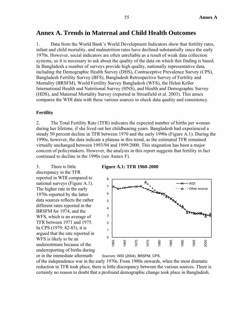
55 Annex A

Annex A. Trends in Maternal and Child Health Outcomes

1. Data from the World Bank’s World Development Indicators show that fertility rates, infant and child mortality, and malnutrition rates have declined substantially since the early 1970s. However, social indicators are often unreliable as a result of weak data collection systems, so it is necessary to ask about the quality of the data on which this finding is based. In Bangladesh a number of surveys provide high quality, nationally representative data, including the Demographic Health Survey (DHS), Contraceptive Prevalence Survey (CPS), Bangladesh Fertility Survey (BFS), Bangladesh Retrospective Survey of Fertility and Mortality (BRSFM), World Fertility Survey Bangladesh (WFS), the Helen Keller International Health and Nutritional Survey (HNS), and Health and Demographic Survey (HDS), and Maternal Mortality Survey (reported in Streatfield et al. 2003). This annex compares the WDI data with these various sources to check data quality and consistency.

Fertility

2. The Total Fertility Rate (TFR) indicates the expected number of births per woman during her lifetime, if she lived out her childbearing years. Bangladesh had experienced a steady 50 percent decline in TFR between 1970 and the early 1990s (Figure A.1). During the 1990s, however, the data indicate a plateau in this trend, as the estimated TFR remained virtually unchanged between 1993/94 and 1999/2000. This stagnation has been a major concern of policymakers. However, the analysis in this report suggests that fertility in fact continued to decline in the 1990s (see Annex F).

3. There is little discrepancy in the TFR reported in WDI compared to national surveys (Figure A.1). The higher rate in the early 1970s reported by the latter data sources reflects the rather different rates reported in the BRSFM for 1974, and the WFS, which is an average of TFR between 1971 and 1975. In CPS (1979: 82-83), it is argued that the rate reported in WFS is likely to be an underestimate because of the underreporting of births during or in the immediate aftermath of the independence war in the early 1970s. From 1980s onwards, when the most dramatic reduction in TFR took place, there is little discrepancy between the various sources. There is certainly no reason to doubt that a profound demographic change took place in Bangladesh.

Figure A.1: TFR 1960-2000

0

1

2

3

4

5

6

7

8

1960

1965

1970

1975

1980

1985

1990

1995

2000

WDIOther source

Sources: WDI (2004), BRSFM, CPS.

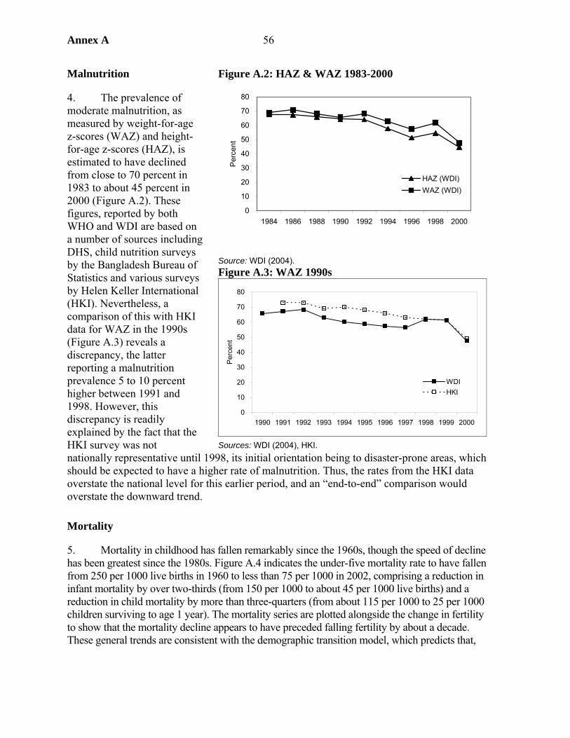
Annex A 56

Malnutrition

4. The prevalence of moderate malnutrition, as measured by weight-for-age z-scores (WAZ) and height-for-age z-scores (HAZ), is estimated to have declined from close to 70 percent in 1983 to about 45 percent in 2000 (Figure A.2). These figures, reported by both WHO and WDI are based on a number of sources including DHS, child nutrition surveys by the Bangladesh Bureau of Statistics and various surveys by Helen Keller International (HKI). Nevertheless, a comparison of this with HKI data for WAZ in the 1990s (Figure A.3) reveals a discrepancy, the latter reporting a malnutrition prevalence 5 to 10 percent higher between 1991 and 1998. However, this discrepancy is readily explained by the fact that the HKI survey was not nationally representative until 1998, its initial orientation being to disaster-prone areas, which should be expected to have a higher rate of malnutrition. Thus, the rates from the HKI data overstate the national level for this earlier period, and an “end-to-end” comparison would overstate the downward trend.

Mortality

5. Mortality in childhood has fallen remarkably since the 1960s, though the speed of decline has been greatest since the 1980s. Figure A.4 indicates the under-five mortality rate to have fallen from 250 per 1000 live births in 1960 to less than 75 per 1000 in 2002, comprising a reduction in infant mortality by over two-thirds (from 150 per 1000 to about 45 per 1000 live births) and a reduction in child mortality by more than three-quarters (from about 115 per 1000 to 25 per 1000 children surviving to age 1 year). The mortality series are plotted alongside the change in fertility to show that the mortality decline appears to have preceded falling fertility by about a decade. These general trends are consistent with the demographic transition model, which predicts that,

Figure A.2: HAZ & WAZ 1983-2000

Source: WDI (2004). Figure A.3: WAZ 1990s

0

10

20

30

40

50

60

70

80

1990 1991 1992 1993 1994 1995 1996 1997 1998 1999 2000

Per

cent

WDIHKI

Sources: WDI (2004), HKI.

0

10

20

30

40

50

60

70

80

1984 1986 1988 1990 1992 1994 1996 1998 2000P

erce

nt

HAZ (WDI)WAZ (WDI)

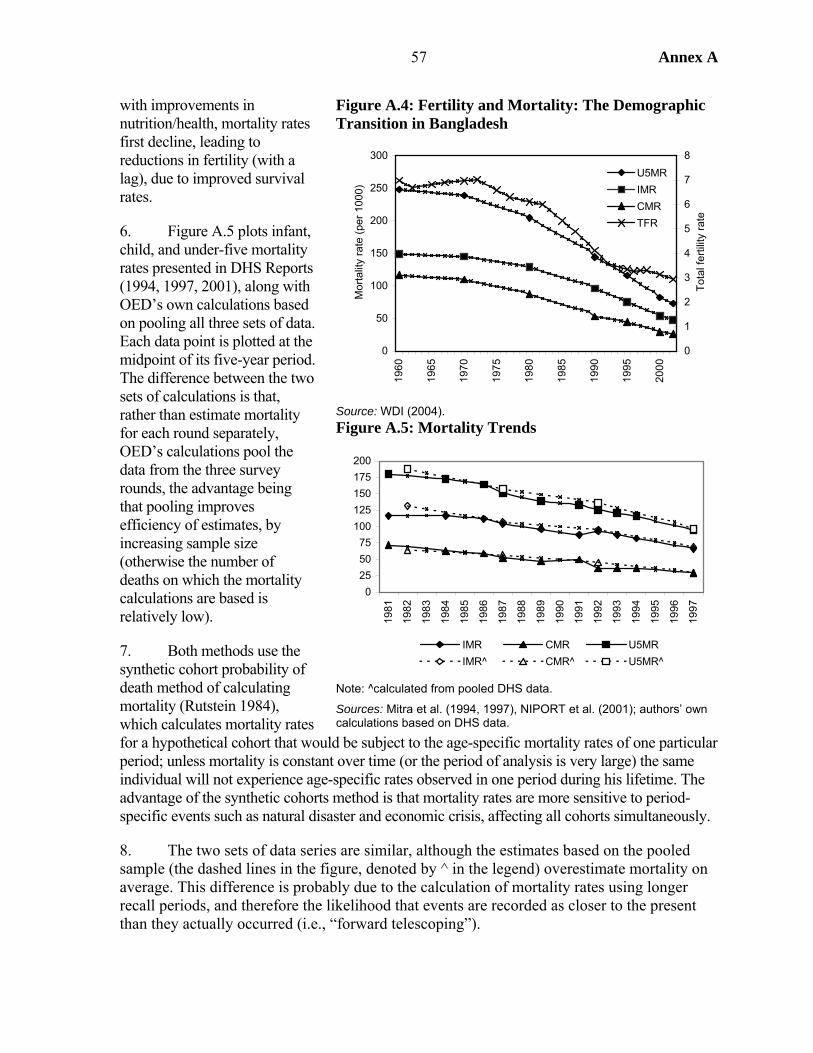
57 Annex A

with improvements in nutrition/health, mortality rates first decline, leading to reductions in fertility (with a lag), due to improved survival rates.

6. Figure A.5 plots infant, child, and under-five mortality rates presented in DHS Reports (1994, 1997, 2001), along with OED’s own calculations based on pooling all three sets of data. Each data point is plotted at the midpoint of its five-year period. The difference between the two sets of calculations is that, rather than estimate mortality for each round separately, OED’s calculations pool the data from the three survey rounds, the advantage being that pooling improves efficiency of estimates, by increasing sample size (otherwise the number of deaths on which the mortality calculations are based is relatively low).

7. Both methods use the synthetic cohort probability of death method of calculating mortality (Rutstein 1984), which calculates mortality rates for a hypothetical cohort that would be subject to the age-specific mortality rates of one particular period; unless mortality is constant over time (or the period of analysis is very large) the same individual will not experience age-specific rates observed in one period during his lifetime. The advantage of the synthetic cohorts method is that mortality rates are more sensitive to period-specific events such as natural disaster and economic crisis, affecting all cohorts simultaneously.

8. The two sets of data series are similar, although the estimates based on the pooled sample (the dashed lines in the figure, denoted by ^ in the legend) overestimate mortality on average. This difference is probably due to the calculation of mortality rates using longer recall periods, and therefore the likelihood that events are recorded as closer to the present than they actually occurred (i.e., “forward telescoping”).

Figure A.4: Fertility and Mortality: The Demographic Transition in Bangladesh

0

50

100

150

200

250

300

1960

1965

1970

1975

1980

1985

1990

1995

2000

Mor

talit

y ra

te (p

er 1

000)

0

1

2

3

4

5

6

7

8

Tot

al fe

rtilit

y ra

te

U5MRIMRCMRTFR

Source: WDI (2004). Figure A.5: Mortality Trends

0255075

100125150175200

1981

1982

1983

1984

1985

1986

1987

1988

1989

1990

1991

1992

1993

1994

1995

1996

1997

IMR CMR U5MRIMR^ CMR^ U5MR^

Note: ^calculated from pooled DHS data.

Sources: Mitra et al. (1994, 1997), NIPORT et al. (2001); authors’ own calculations based on DHS data.

Annex B 58

Annex B. Cross-Country Analysis of Child Health and Nutrition Outcomes

1. Some initial insights regarding the main determinants of child health and nutritional outcomes can be sought from cross-country regressions. This is not a novel area of analysis. Work emanating from the World Bank (Reutlinger and Selowsky 1976, and Berg 1983), and followed up more recently in a series of papers by Haddad and others (e.g., Smith and Haddad 2000), has shown that income growth translates into improved nutritional status, but at too low a rate to achieve international targets. Concerning mortality, there has also been debate about the respective role of economic growth versus direct support for lower mortality via health service provision (e.g., Filmer and Pritchett 1999 and the debate around the World Health Report 2000; see Pedersen 2002).

2. This annex presents cross-country regression results drawing on two data sources. The first set of data updates the work of Haddad and Smith, using the same sources and series, but including more recent data. Their main results are replicated, and extended through the addition of further variables and a closer look at the non-income drivers of changes in nutritional outcomes specifically for the case of Bangladesh. DHS data, usually used for the sort of household modeling presented in Annexes C and D of this report, can also be used for cross-country analysis, using national averages of the various variables, which are provided on the Macro International website. These second set of estimates are provided to corroborate the first set of results, and as some additional variables can be included.

Drivers of Maternal and Child Health and Nutritional Outcomes in Bangladesh

3. Smith and Haddad (2000) estimate two sets of models for the determinants of the proportion of children who are underweight, using a cross-country data set culled from various sources. The first model regresses nutritional status on what they call the “basic determinants” of per capita GDP and democracy (measured by the Freedom House political freedom index). The second model, of underlying determinants, includes access to safe water, female secondary school enrollments, the ratio of male to female life expectancy, as a measure of gender inequality, and per capita dietary energy supply. The logic of the approach is that the latter variables, which directly affect nutritional status, depend in turn (though only in part) on the “basic determinants.” The basic determinants equation is thus a reduced-form equation, though one which appears to suffer from omitted variable bias, as there are other determinants of the underlying variables than GDP and democracy alone. Using the results from a fixed-effects estimate of their underlying determinants model they examine the relative importance of the different variables in the explained change in nutrition. Female education comes out as the most important factor (43 percent), followed by food supply (21 percent), and then health environment (safe water, 19 percent) and finally women’s status (11 percent).

4. The analysis for this report has updated their data set with five modifications: (1) the analysis is carried out for four dependent variables: HAZ, WAZ, under-five mortality, and the total fertility rate; (2) more recent data have been obtained; (3) rather than using data for specific years, decade averages are used for the 1970s, '80s, '90s, and the current decade; (4) female literacy is used rather than secondary enrollment, as the stock of female education

Annex B 59

appears more appropriate than the new flow into that stock, which is what the enrollment rate measures; (5) income inequality has been added to the data set, although this variable restricts sample size so that estimates are presented with and without the variable. As in Smith and Haddad, results are presented from both ordinary least squares (OLS) and fixed effects (FE) models, using time dummies in the latter and regional and time dummies in the former.

5. The results from the “basic determinants” model demonstrate the extent to which income growth has been behind improvements in maternal and child health and nutrition outcomes. There are both direct and indirect channels from income to better health and nutrition. The direct channel is from the higher consumption of food and health services made possible by higher income. Indirect channels include increasing both the supply and demand for education, improved water supply, and other facilities. To the extent that factors positively affecting health and nutrition outcomes are positively correlated with income, but not wholly explained by income, then the regression of any one outcome on income will provide an upward biased estimate of the income effect, which may be regarded as an “upper limit” estimate of this effect.

6. Table B.1 shows the extent to which income growth in Bangladesh has determined the change in the four outcomes being considered here. The results are based on the model 1 OLS estimates for each variable, shown in Tables B.2(a)-B.5(a). Multiplying the coefficient on income by the change in Bangladesh’s (log) income gives the change in the outcome, e.g., under-five mortality, attributable to the income effect. This effect is highest in the case of mortality, in which case it is just under one-third, and lowest in the case of fertility, where it is just 16 percent.

Table B.1: Income Growth Accounts for at Most One-Third of the Reduction in Mortality in Bangladesh… And Less Than a Fifth of Lower Fertility

1980

actual 2000

actual

2000 income- based

estimate

Percent reduction

explained by income

Under-five mortality 205.0 77.5 163.1 32.9 Total fertility rate 5.6 3.0 5.2 16.0 Stunting 67.6 44.7 62.3 23.1 Underweight 69.5 47.7 64.6 22.4

Source: Calculated from data used for Figure B.1 7. The same argument may be made graphically, as is done in Figure B.1. The four graphs in Figure B.1 show this clear link between income and four social outcomes – under-five mortality, the total fertility rate, and the prevalence of stunting and underweight among under-fives – using the cross-section data.

8. In the 1980s, Bangladesh lay above the fitted line (the solid line in each figure) for under-five mortality and fertility, meaning that those indicators were worse than should be expected for a country at its income level. If these indicators had improved following the internationally established relationship with income, then subsequent observations for

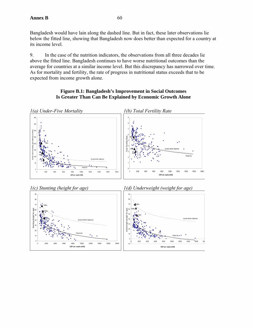
Annex B 60

Bangladesh would have lain along the dashed line. But in fact, these later observations lie below the fitted line, showing that Bangladesh now does better than expected for a country at its income level.

9. In the case of the nutrition indicators, the observations from all three decades lie above the fitted line. Bangladesh continues to have worse nutritional outcomes than the average for countries at a similar income level. But this discrepancy has narrowed over time. As for mortality and fertility, the rate of progress in nutritional status exceeds that to be expected from income growth alone.

Figure B.1: Bangladesh’s Improvement in Social Outcomes Is Greater Than Can Be Explained by Economic Growth Alone

1(a) Under-Five Mortality 1(b) Total Fertility Rate

0

50

100

150

200

250

300

350

400

0 2000 4000 6000 8000 10000 12000 14000 16000 18000


Und

er fi

ve m

orta

lity

(per

000

live

birt

hs)

1980s

1990s

2000

Fitted line


0

1

2

3

4

5

6

7

8

9

0 2000 4000 6000 8000 10000 12000 14000 16000 18000


Tota

l Fer

tility

Rat

e 1980s

1990s

2000sFitted line

Income driven trajectory

1(c) Stunting (height for age)

1(d) Underweight (weight for age)

0

10

20

30

40

50

60

70

80

90

0 2000 4000 6000 8000 10000 12000 14000 16000 18000


Stun

ting

(hei

ght f

or a

ge)

1980s

1990s

2000

Fitted line


-10

0

10

20

30

40

50

60

70

80

90

0 2000 4000 6000 8000 10000 12000 14000 16000 180


Und

erw

eigh

t (w

eigh

t for

age

)

1980s

1990s

2000

Fitted line


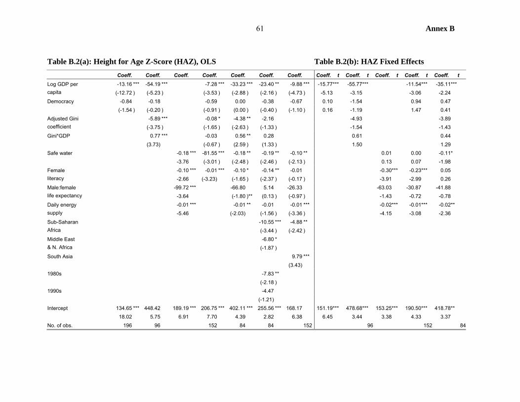
Annex B 61

Table B.2(a): Height for Age Z-Score (HAZ), OLS Table B.2(b): HAZ Fixed Effects Coeff. Coeff. Coeff. Coeff. Coeff. Coeff. Coeff. Coeff. t Coeff. t Coeff. t Coeff. t Coeff. t

-13.16 *** -54.19 *** -7.28 *** -33.23 *** -23.40 ** -9.88 *** -15.77*** -55.77*** -11.54*** -35.11*** Log GDP per capita (-12.72 ) (-5.23 ) (-3.53 ) (-2.88 ) (-2.16 ) (-4.73 ) -5.13 -3.15 -3.06 -2.24 Democracy -0.84 -0.18 -0.59 0.00 -0.38 -0.67 0.10 -1.54 0.94 0.47 (-1.54 ) (-0.20 ) (-0.91 ) (0.00 ) (-0.40 ) (-1.10 ) 0.16 -1.19 1.47 0.41

-5.89 *** -0.08 * -4.38 ** -2.16 -4.93 -3.89 Adjusted Gini coefficient (-3.75 ) (-1.65 ) (-2.63 ) (-1.33 ) -1.54 -1.43 Gini*GDP 0.77 *** -0.03 0.56 ** 0.28 0.61 0.44 (3.73) (-0.67 ) (2.59 ) (1.33 ) 1.50 1.29 Safe water -0.18 *** -81.55 *** -0.18 ** -0.19 ** -0.10 ** 0.01 0.00 -0.11* -3.76 (-3.01 ) (-2.48 ) (-2.46 ) (-2.13 ) 0.13 0.07 -1.98

-0.10 *** -0.01 *** -0.10 * -0.14 ** -0.01 -0.30*** -0.23*** 0.05 Female literacy -2.66 (-3.23) (-1.65 ) (-2.37 ) (-0.17 ) -3.91 -2.99 0.26

-99.72 *** -66.80 5.14 -26.33 -63.03 -30.87 -41.88 Male:female life expectancy -3.64 (-1.80 )** (0.13 ) (-0.97 ) -1.43 -0.72 -0.78

-0.01 *** -0.01 ** -0.01 -0.01 *** -0.02*** -0.01*** -0.02** Daily energy supply -5.46 (-2.03) (-1.56 ) (-3.36 ) -4.15 -3.08 -2.36

-10.55 *** -4.88 ** Sub-Saharan Africa (-3.44 ) (-2.42 )

-6.80 * Middle East & N. Africa (-1.87 ) South Asia 9.79 *** (3.43) 1980s -7.83 ** (-2.18 ) 1990s -4.47 (-1.21) Intercept 134.65 *** 448.42 189.19 *** 206.75 *** 402.11 *** 255.56 *** 168.17 151.19*** 478.68*** 153.25*** 190.50*** 418.78** 18.02 5.75 6.91 7.70 4.39 2.82 6.38 6.45 3.44 3.38 4.33 3.37 No. of obs. 196 96 152 84 84 152 96 152 84

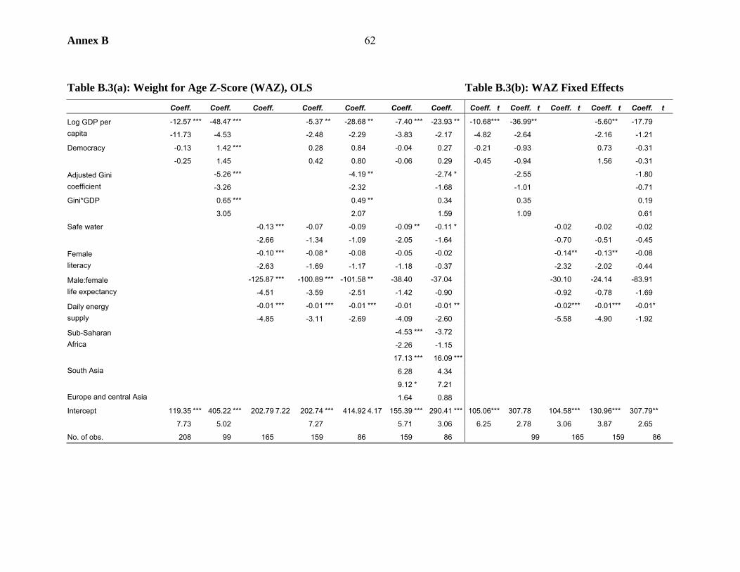
Annex B 62

Table B.3(a): Weight for Age Z-Score (WAZ), OLS Table B.3(b): WAZ Fixed Effects

Coeff. Coeff. Coeff. Coeff. Coeff. Coeff. Coeff. Coeff. t Coeff. t Coeff. t Coeff. t Coeff. t

-12.57 *** -48.47 *** -5.37 ** -28.68 ** -7.40 *** -23.93 ** -10.68*** -36.99** -5.60** -17.79 Log GDP per capita -11.73 -4.53 -2.48 -2.29 -3.83 -2.17 -4.82 -2.64 -2.16 -1.21

Democracy -0.13 1.42 *** 0.28 0.84 -0.04 0.27 -0.21 -0.93 0.73 -0.31

-0.25 1.45 0.42 0.80 -0.06 0.29 -0.45 -0.94 1.56 -0.31

-5.26 *** -4.19 ** -2.74 * -2.55 -1.80 Adjusted Gini coefficient -3.26 -2.32 -1.68 -1.01 -0.71

Gini*GDP 0.65 *** 0.49 ** 0.34 0.35 0.19

3.05 2.07 1.59 1.09 0.61

Safe water -0.13 *** -0.07 -0.09 -0.09 ** -0.11 * -0.02 -0.02 -0.02

-2.66 -1.34 -1.09 -2.05 -1.64 -0.70 -0.51 -0.45

-0.10 *** -0.08 * -0.08 -0.05 -0.02 -0.14** -0.13** -0.08 Female literacy -2.63 -1.69 -1.17 -1.18 -0.37 -2.32 -2.02 -0.44

-125.87 *** -100.89 *** -101.58 ** -38.40 -37.04 -30.10 -24.14 -83.91 Male:female life expectancy -4.51 -3.59 -2.51 -1.42 -0.90 -0.92 -0.78 -1.69

-0.01 *** -0.01 *** -0.01 *** -0.01 -0.01 ** -0.02*** -0.01*** -0.01* Daily energy supply -4.85 -3.11 -2.69 -4.09 -2.60 -5.58 -4.90 -1.92

-4.53 *** -3.72 Sub-Saharan Africa -2.26 -1.15

17.13 *** 16.09 *** South Asia 6.28 4.34

9.12 * 7.21 Europe and central Asia 1.64 0.88

Intercept 119.35 *** 405.22 *** 202.79 7.22 202.74 *** 414.92 4.17 155.39 *** 290.41 *** 105.06*** 307.78 104.58*** 130.96*** 307.79**

7.73 5.02 7.27 5.71 3.06 6.25 2.78 3.06 3.87 2.65

No. of obs. 208 99 165 159 86 159 86 99 165 159 86

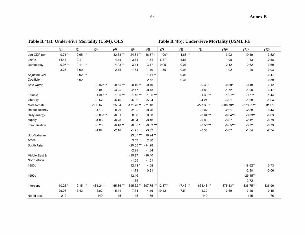
Annex B 63

Table B.4(a): Under-Five Mortality (U5M), OLS Table B.4(b): Under-Five Mortality (U5M), FE

(1) (2) (3) (4) (5) (6) (7) (8) (9) (10) (11) (12) -0.71 *** -0.65 *** -32.38 *** -24.84 *** -16.57 * -1.00*** -1.66 *** 13.92 19.19 13.52* Log GDP per

capita -14.45 -9.11 -4.45 -3.54 -1.71 -6.37 -5.58 1.08 1.53 0.58 Democracy -0.08 *** -0.11 *** 4.98 ** 3.11 -3.17 -0.05 -0.07 -2.12 -2.62 -3.60 -3.27 -3.00 2.45 1.64 -1.19 -1.55 -0.98 -1.02 -1.29 -0.93

0.02 *** 1.11 ** 0.01 -0.47 Adjusted Gini Coefficient 3.02 2.52 0.31 -0.39 Safe water -0.92 *** -0.65 *** -0.40 ** -0.10 -0.33* -0.30* -0.18 0.12 -5.04 -3.25 -2.17 -0.43 -1.85 -1.72 -1.00 0.47

-1.34 *** -1.06 *** -1.10 *** -1.05 *** -1.33*** -1.27*** -0.77* -1.44 Female Literacy -9.62 -6.46 -6.62 -5.34 -4.21 -3.61 -1.98 -1.04

-100.67 25.34 -171.70 ** -71.48 -277.36** -308.70** -378.51*** 81.01 Male:female life expectancy -1.13 0.29 -2.05 -0.70 -2.02 -2.31 -2.88 0.44

-0.03 *** -0.01 0.00 0.00 -0.04*** -0.04*** -0.03** -0.03 Daily energy supply -4.00 -0.90 -0.34 -0.40 -2.98 -3.07 -2.12 -0.79 Immunization -0.20 -0.40 ** -0.35 * -0.83 *** -0.55*** -0.65*** -0.32 -0.79 -1.04 -2.16 -1.75 -3.39 -3.35 -3.87 -1.54 -2.34

23.37 *** 18.94 ** Sub-Saharan Africa 3.57 2.30 South Asia -29.05 *** -14.28 -2.98 -1.34

-15.87 -16.40 Middle East & North Africa -1.55 -1.51 1980s -12.11 * 4.09 -18.62** -0.73 -1.78 0.51 -2.50 -0.06 1990s -12.46 -26.15*** -1.65 -2.72 Intercept 10.23 *** 9.15 *** 451.24 *** 465.86 *** 595.32 *** 397.75 *** 12.37*** 17.43 *** 638.48*** 575.33*** 536.75*** 136.90 29.08 16.42 5.02 5.44 7.31 4.16 10.42 7.54 4.30 3.59 3.46 0.45 No. of obs. 212 149 145 145 76 149 145 76

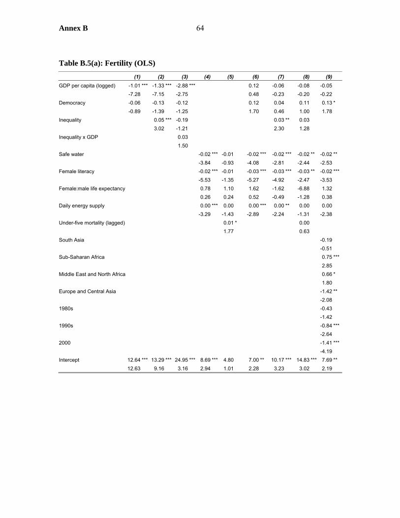
Annex B 64

Table B.5(a): Fertility (OLS)

(1) (2) (3) (4) (5) (6) (7) (8) (9)-1.01 *** -1.33 *** -2.88 *** 0.12 -0.06 -0.08 -0.05 GDP per capita (logged) -7.28 -7.15 -2.75 0.48 -0.23 -0.20 -0.22

Democracy -0.06 -0.13 -0.12 0.12 0.04 0.11 0.13 * -0.89 -1.39 -1.25 1.70 0.46 1.00 1.78 Inequality 0.05 *** -0.19 0.03 ** 0.03 3.02 -1.21 2.30 1.28

0.03 Inequality x GDP 1.50

Safe water -0.02 *** -0.01 -0.02 *** -0.02 *** -0.02 ** -0.02 ** -3.84 -0.93 -4.08 -2.81 -2.44 -2.53 Female literacy -0.02 *** -0.01 -0.03 *** -0.03 *** -0.03 ** -0.02 *** -5.53 -1.35 -5.27 -4.92 -2.47 -3.53

0.78 1.10 1.62 -1.62 -6.88 1.32 Female:male life expectancy 0.26 0.24 0.52 -0.49 -1.28 0.38 0.00 *** 0.00 0.00 *** 0.00 ** 0.00 0.00 Daily energy supply -3.29 -1.43 -2.89 -2.24 -1.31 -2.38 0.01 * 0.00 Under-five mortality (lagged) 1.77 0.63

South Asia -0.19 -0.51

0.75 ***Sub-Saharan Africa 2.85 0.66 * Middle East and North Africa 1.80 -1.42 ** Europe and Central Asia -2.08

1980s -0.43 -1.42 1990s -0.84 *** -2.64 2000 -1.41 *** -4.19 Intercept 12.64 *** 13.29 *** 24.95 *** 8.69 *** 4.80 7.00 ** 10.17 *** 14.83 *** 7.69 ** 12.63 9.16 3.16 2.94 1.01 2.28 3.23 3.02 2.19

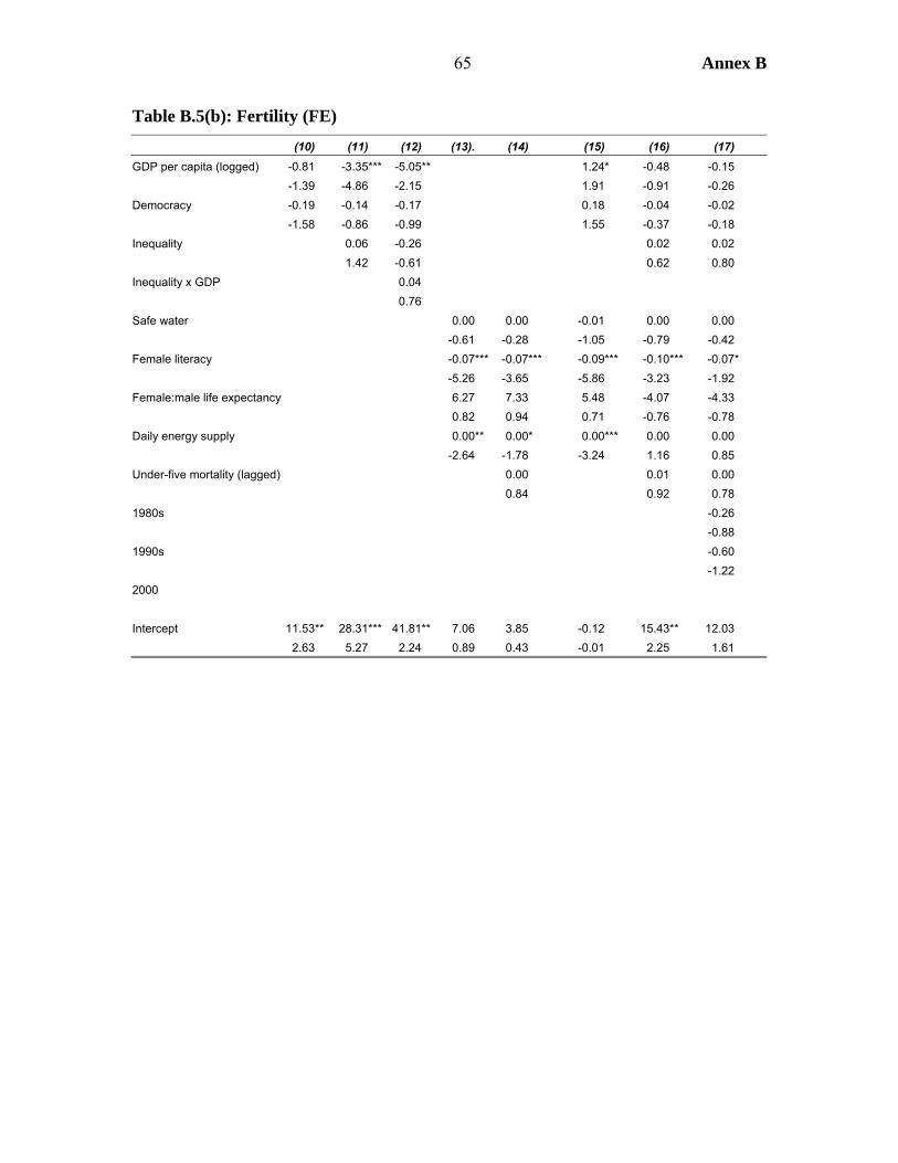
65 Annex B

Table B.5(b): Fertility (FE)

(10) (11) (12) (13). (14) (15) (16) (17)-0.81 -3.35*** -5.05** 1.24* -0.48 -0.15 GDP per capita (logged) -1.39 -4.86 -2.15 1.91 -0.91 -0.26

Democracy -0.19 -0.14 -0.17 0.18 -0.04 -0.02 -1.58 -0.86 -0.99 1.55 -0.37 -0.18 Inequality 0.06 -0.26 0.02 0.02 1.42 -0.61 0.62 0.80

0.04 Inequality x GDP 0.76

Safe water 0.00 0.00 -0.01 0.00 0.00 -0.61 -0.28 -1.05 -0.79 -0.42 Female literacy -0.07*** -0.07*** -0.09*** -0.10*** -0.07* -5.26 -3.65 -5.86 -3.23 -1.92

6.27 7.33 5.48 -4.07 -4.33 Female:male life expectancy 0.82 0.94 0.71 -0.76 -0.78 0.00** 0.00* 0.00*** 0.00 0.00 Daily energy supply -2.64 -1.78 -3.24 1.16 0.85 0.00 0.01 0.00 Under-five mortality (lagged) 0.84 0.92 0.78

1980s -0.26 -0.88 1990s -0.60 -1.22 2000 Intercept 11.53** 28.31*** 41.81** 7.06 3.85 -0.12 15.43** 12.03 2.63 5.27 2.24 0.89 0.43 -0.01 2.25 1.61

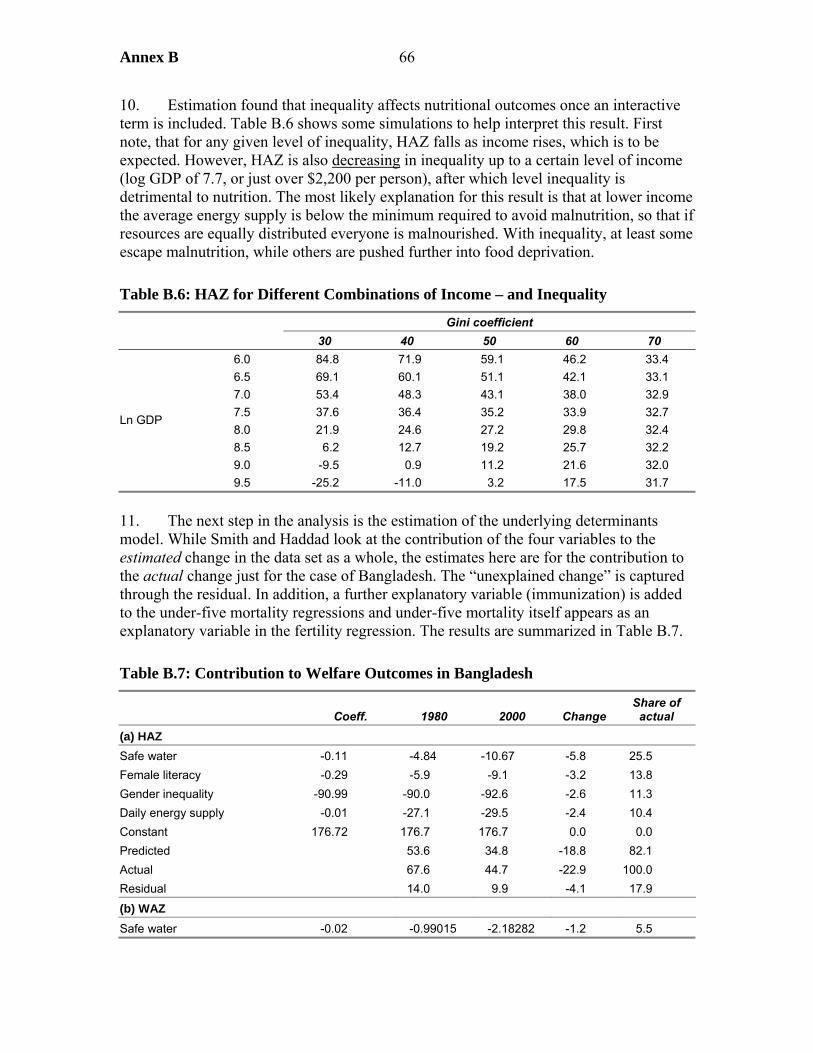
Annex B 66

10. Estimation found that inequality affects nutritional outcomes once an interactive term is included. Table B.6 shows some simulations to help interpret this result. First note, that for any given level of inequality, HAZ falls as income rises, which is to be expected. However, HAZ is also decreasing in inequality up to a certain level of income (log GDP of 7.7, or just over $2,200 per person), after which level inequality is detrimental to nutrition. The most likely explanation for this result is that at lower income the average energy supply is below the minimum required to avoid malnutrition, so that if resources are equally distributed everyone is malnourished. With inequality, at least some escape malnutrition, while others are pushed further into food deprivation.

Table B.6: HAZ for Different Combinations of Income – and Inequality

Gini coefficient 30 40 50 60 70

6.0 84.8 71.9 59.1 46.2 33.4 6.5 69.1 60.1 51.1 42.1 33.1 7.0 53.4 48.3 43.1 38.0 32.9 7.5 37.6 36.4 35.2 33.9 32.7 8.0 21.9 24.6 27.2 29.8 32.4 8.5 6.2 12.7 19.2 25.7 32.2 9.0 -9.5 0.9 11.2 21.6 32.0

Ln GDP

9.5 -25.2 -11.0 3.2 17.5 31.7

11. The next step in the analysis is the estimation of the underlying determinants model. While Smith and Haddad look at the contribution of the four variables to the estimated change in the data set as a whole, the estimates here are for the contribution to the actual change just for the case of Bangladesh. The “unexplained change” is captured through the residual. In addition, a further explanatory variable (immunization) is added to the under-five mortality regressions and under-five mortality itself appears as an explanatory variable in the fertility regression. The results are summarized in Table B.7.

Table B.7: Contribution to Welfare Outcomes in Bangladesh

Coeff. 1980 2000 Change Share of

actual (a) HAZ Safe water -0.11 -4.84 -10.67 -5.8 25.5 Female literacy -0.29 -5.9 -9.1 -3.2 13.8 Gender inequality -90.99 -90.0 -92.6 -2.6 11.3 Daily energy supply -0.01 -27.1 -29.5 -2.4 10.4 Constant 176.72 176.7 176.7 0.0 0.0 Predicted 53.6 34.8 -18.8 82.1 Actual 67.6 44.7 -22.9 100.0 Residual 14.0 9.9 -4.1 17.9

(b) WAZ Safe water -0.02 -0.99015 -2.18282 -1.2 5.5

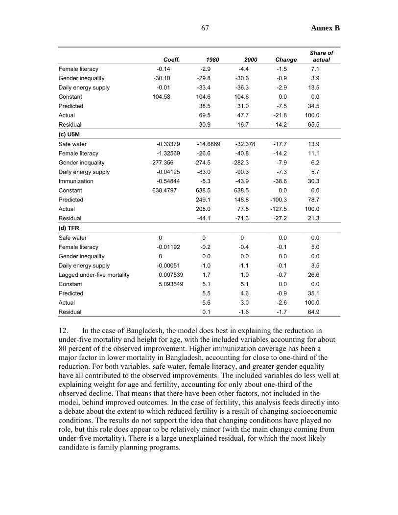
67 Annex B

Coeff. 1980 2000 Change Share of

actual Female literacy -0.14 -2.9 -4.4 -1.5 7.1 Gender inequality -30.10 -29.8 -30.6 -0.9 3.9 Daily energy supply -0.01 -33.4 -36.3 -2.9 13.5 Constant 104.58 104.6 104.6 0.0 0.0 Predicted 38.5 31.0 -7.5 34.5 Actual 69.5 47.7 -21.8 100.0 Residual 30.9 16.7 -14.2 65.5 (c) U5M Safe water -0.33379 -14.6869 -32.378 -17.7 13.9 Female literacy -1.32569 -26.6 -40.8 -14.2 11.1 Gender inequality -277.356 -274.5 -282.3 -7.9 6.2 Daily energy supply -0.04125 -83.0 -90.3 -7.3 5.7 Immunization -0.54844 -5.3 -43.9 -38.6 30.3 Constant 638.4797 638.5 638.5 0.0 0.0 Predicted 249.1 148.8 -100.3 78.7 Actual 205.0 77.5 -127.5 100.0 Residual -44.1 -71.3 -27.2 21.3 (d) TFR Safe water 0 0 0 0.0 0.0 Female literacy -0.01192 -0.2 -0.4 -0.1 5.0 Gender inequality 0 0.0 0.0 0.0 0.0 Daily energy supply -0.00051 -1.0 -1.1 -0.1 3.5 Lagged under-five mortality 0.007539 1.7 1.0 -0.7 26.6 Constant 5.093549 5.1 5.1 0.0 0.0 Predicted 5.5 4.6 -0.9 35.1 Actual 5.6 3.0 -2.6 100.0 Residual 0.1 -1.6 -1.7 64.9

12. In the case of Bangladesh, the model does best in explaining the reduction in under-five mortality and height for age, with the included variables accounting for about 80 percent of the observed improvement. Higher immunization coverage has been a major factor in lower mortality in Bangladesh, accounting for close to one-third of the reduction. For both variables, safe water, female literacy, and greater gender equality have all contributed to the observed improvements. The included variables do less well at explaining weight for age and fertility, accounting for only about one-third of the observed decline. That means that there have been other factors, not included in the model, behind improved outcomes. In the case of fertility, this analysis feeds directly into a debate about the extent to which reduced fertility is a result of changing socioeconomic conditions. The results do not support the idea that changing conditions have played no role, but this role does appear to be relatively minor (with the main change coming from under-five mortality). There is a large unexplained residual, for which the most likely candidate is family planning programs.

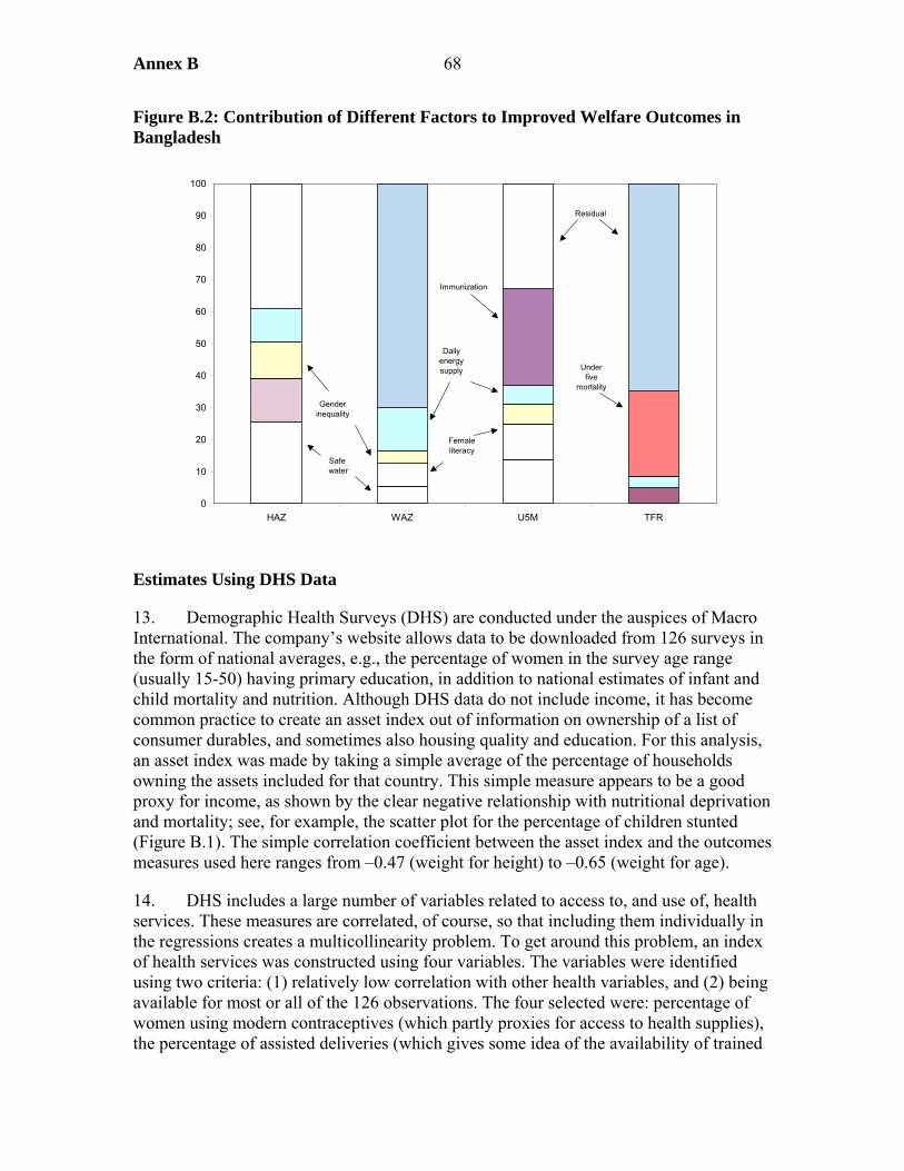
Annex B 68

Figure B.2: Contribution of Different Factors to Improved Welfare Outcomes in Bangladesh

Estimates Using DHS Data

13. Demographic Health Surveys (DHS) are conducted under the auspices of Macro International. The company’s website allows data to be downloaded from 126 surveys in the form of national averages, e.g., the percentage of women in the survey age range (usually 15-50) having primary education, in addition to national estimates of infant and child mortality and nutrition. Although DHS data do not include income, it has become common practice to create an asset index out of information on ownership of a list of consumer durables, and sometimes also housing quality and education. For this analysis, an asset index was made by taking a simple average of the percentage of households owning the assets included for that country. This simple measure appears to be a good proxy for income, as shown by the clear negative relationship with nutritional deprivation and mortality; see, for example, the scatter plot for the percentage of children stunted (Figure B.1). The simple correlation coefficient between the asset index and the outcomes measures used here ranges from –0.47 (weight for height) to –0.65 (weight for age).

14. DHS includes a large number of variables related to access to, and use of, health services. These measures are correlated, of course, so that including them individually in the regressions creates a multicollinearity problem. To get around this problem, an index of health services was constructed using four variables. The variables were identified using two criteria: (1) relatively low correlation with other health variables, and (2) being available for most or all of the 126 observations. The four selected were: percentage of women using modern contraceptives (which partly proxies for access to health supplies), the percentage of assisted deliveries (which gives some idea of the availability of trained

0

10

20

30

40

50

60

70

80

90

100

HAZ WAZ U5M TFR

Safe water

Female literacy

Gender inequality

Daily energy supply

Immunization

Under five

mortality

Residual

69 Annex B

health workers), and, as measures of ante-natal services, the proportion of women having no antenatal services at all and the proportion receiving no tetanus vaccination. The weights were derived from principal components analysis, the last two variables entering with negative weights as should be expected.

Figure B.3: The Income-Outcome Relationship in Cross-Country DHS Data

0

10

20

30

40

50

60

0 10 20 30 40 50 60 70

Asset index

Stun

ting

(HA

Z<2

SDs)

Choice of Regressors

15. The approach adopted for the nutrition regressions assesses the robustness of the coefficients of the various variables. Table B.8 shows the simple regression estimate for each of the variables (equations 1-4 in Table B.8), and the results when all variables are included in a single multiple regression (equation 5 in the table). In addition, to pursue a robust regression approach, all possible pairs and triplets of these variables were estimated. The main findings are as follows:

• The asset index is always significant in the simple regression, but never so in the multiple regression. Indeed, assets are not significant in two of the four regressions with three regressors for both HAZ and WHZ and once for WAZ. This result means that the effect of assets found in the simple regression is picking up the impact of the other omitted variables which are correlated with assets, which they all are, but particularly the education variables. Of course the correlation with assets is in this case likely be at least in part since income (for which assets are proxying) is one determinant of education.

Annex B 70

• Health service inputs remain significant in two of the three nutrition equations, the exception being wasting (weight for height), the latter being the only case when the health index is not significant in any of the other regessions (it is not so in two of the four triplets for this regressand).

• The education variable is significant in all regressions. In the case of HAZ, secondary education worked better than primary and so was used instead.1

• The various access to media variables were each tried, retaining in each case that which best fit for that dependent variable: watching TV for HAZ and WHZ and reading the newspaper for WAZ. These variables are significant in the multiple regressions (for WHZ only when the South Asia dummy is added, though the dummy just removes the significance of the newspaper variable in the WAZ equation).

• The South Asia dummy (added in equation 6 of Table B.8 for each regressand) is always significantly positive, showing the worse nutritional status of that region once a range of determinants are allowed for.

16. These results were used as point estimates to model the drivers of change in nutritional status. The calculations were performed as follows:

• For each variable, Table B.9 records the quartile values of the regressors. • These regressors are used to calculate the expected value of the dependent

variable, for a country with the respective set of characteristics. Although they need not be exactly equal, the corresponding values do correspond quite closely to the quartile values for the appropriate outcome variable in each case.

• The absolute change is the change in the outcome that would be caused by a country moving from across the inter-quartile range. This figure is calculated as the product of the difference in the value of the independent variable and the estimated coefficient. These changes sum to the predicted change in the outcome variable. Hence, the changes from each separate regressor can be expressed as a percentage of the total change.

17. The results show that the smallest effect usually comes from the change in the asset index (which recall was anyhow insignificant), with education and media accounting for the bulk of the difference for the first two outcomes. In these first two cases, health care accounts for a bit under 20 percent of the difference, and rather more for WAZ, for which assets also appear more important.

1. In the multiple regression for HAZ primary education in fact has the wrong sign, though it is not significant.

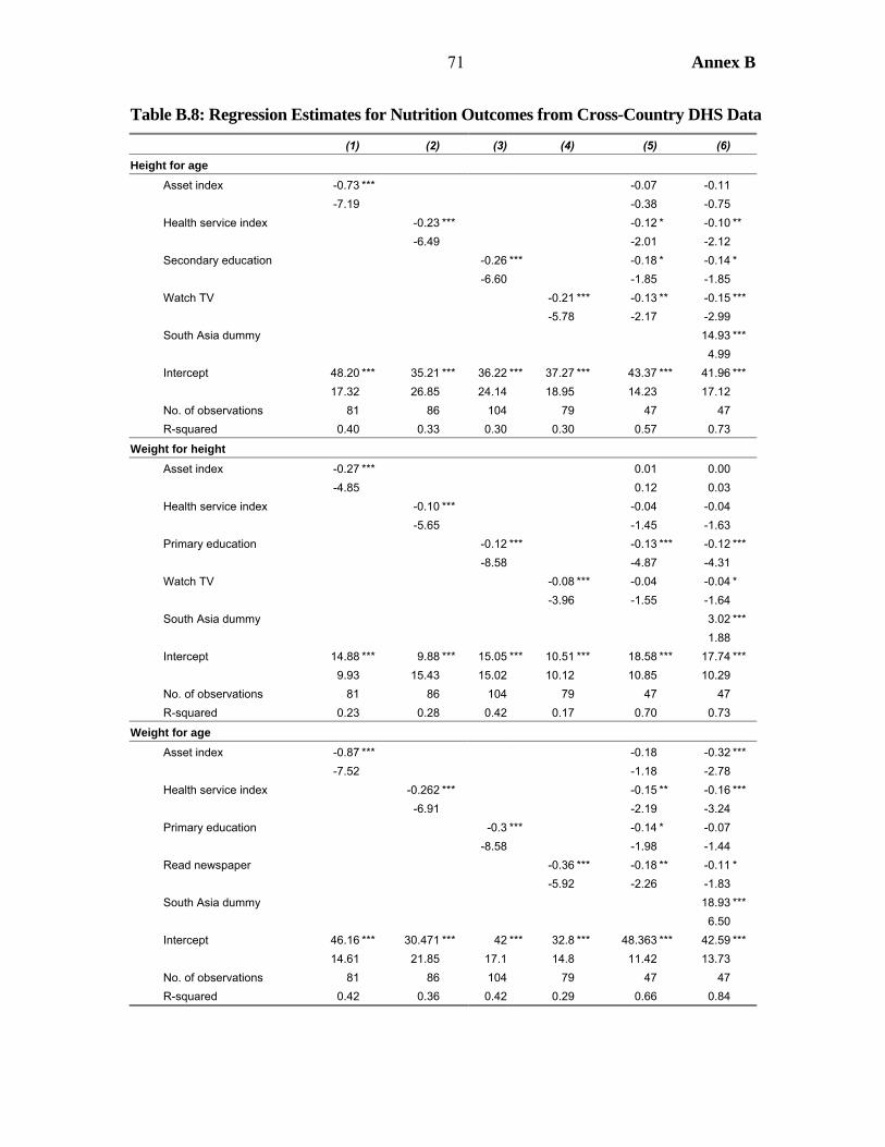
71 Annex B

Table B.8: Regression Estimates for Nutrition Outcomes from Cross-Country DHS Data

(1) (2) (3) (4) (5) (6) Height for age Asset index -0.73 *** -0.07 -0.11 -7.19 -0.38 -0.75 Health service index -0.23 *** -0.12 * -0.10 ** -6.49 -2.01 -2.12 Secondary education -0.26 *** -0.18 * -0.14 * -6.60 -1.85 -1.85 Watch TV -0.21 *** -0.13 ** -0.15 *** -5.78 -2.17 -2.99 South Asia dummy 14.93 *** 4.99 Intercept 48.20 *** 35.21 *** 36.22 *** 37.27 *** 43.37 *** 41.96 *** 17.32 26.85 24.14 18.95 14.23 17.12 No. of observations 81 86 104 79 47 47 R-squared 0.40 0.33 0.30 0.30 0.57 0.73

Weight for height Asset index -0.27 *** 0.01 0.00 -4.85 0.12 0.03 Health service index -0.10 *** -0.04 -0.04 -5.65 -1.45 -1.63 Primary education -0.12 *** -0.13 *** -0.12 *** -8.58 -4.87 -4.31 Watch TV -0.08 *** -0.04 -0.04 * -3.96 -1.55 -1.64 South Asia dummy 3.02 *** 1.88 Intercept 14.88 *** 9.88 *** 15.05 *** 10.51 *** 18.58 *** 17.74 *** 9.93 15.43 15.02 10.12 10.85 10.29 No. of observations 81 86 104 79 47 47 R-squared 0.23 0.28 0.42 0.17 0.70 0.73

Weight for age Asset index -0.87 *** -0.18 -0.32 *** -7.52 -1.18 -2.78 Health service index -0.262 *** -0.15 ** -0.16 *** -6.91 -2.19 -3.24 Primary education -0.3 *** -0.14 * -0.07 -8.58 -1.98 -1.44 Read newspaper -0.36 *** -0.18 ** -0.11 * -5.92 -2.26 -1.83 South Asia dummy 18.93 *** 6.50 Intercept 46.16 *** 30.471 *** 42 *** 32.8 *** 48.363 *** 42.59 *** 14.61 21.85 17.1 14.8 11.42 13.73 No. of observations 81 86 104 79 47 47 R-squared 0.42 0.36 0.42 0.29 0.66 0.84

Annex B 72

18. What these results show is that improvements in education and access to media (presumably as a medium of health and nutritional advice) can bring about substantial reductions in nutritional deprivation. It may not be accurate to say these reductions can be brought about “independent of income growth” since that growth may be needed to generate both supply and demand for education and media services. Having said that, neither of these variables is driven solely by income, so there is scope for autonomous improvements in nutrition.

Table B.9: Regression-based Estimates of Contribution to Welfare Changes

Coefficient

First quartile Median

Second quartile

Percentage difference

Absolute Share Height for age Asset index -0.11 18.8 23.1 31.6 -1.39 8.3 Health service index -0.10 10.0 26.3 42.2 -3.16 18.9 Secondary education -0.14 12.2 24.3 43.6 -4.55 27.2 Watch TV -0.15 24.9 35.7 77.2 -7.63 45.6 South Asia dummy 14.93 0 0 0 .. .. Intercept 41.96 1 1 1 .. .. Predicted 33.5 28.1 16.8 -16.7 100.0 Weight for height Asset index 0.002 18.8 23.1 31.6 0.03 -0.3 Health service index -0.04 10.0 26.3 42.2 -1.44 16.1 Primary education -0.12 43.3 71.9 89.2 -5.35 60.1 Watch TV -0.04 24.9 35.7 77.2 -2.15 24.1 South Asia dummy 3.02 0 0 0 .. .. Intercept 17.74 1 1 1 .. .. Predicted 11.3 6.8 2.4 -8.9 100.0 Weight for age Asset index -0.32 18.8 23.1 31.6 -4.04 24.5 Health service index -0.16 10.0 26.3 42.2 -5.16 31.3 Primary education -0.07 43.3 71.9 89.2 -3.32 20.1 Read newspaper -0.11 13.1 26.2 49.8 -3.97 24.1 South Asia dummy 18.93 0 0 0 .. .. Intercept 42.59 1 1 1 .. .. Predicted 30.5 23.0 14.0 -16.5 100.0

19. Somewhat similar results emerge for the mortality regressions, although only the multiple regression results are shown here. The dependent variables are neo-natal mortality (first month), post-natal mortality (months 1-11), and child mortality. As with nutrition, assets are significant in a simple regression but never so in the multiple regression. In these regressions it was possible to include both primary and secondary education and get significant results, despite the very high level of correlation between these two regressors. For infants, secondary is significant and primary is not, having even the wrong sign for post-natal mortality (which is also true if secondary is omitted). But

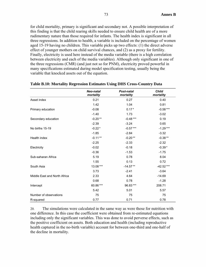
73 Annex B

for child mortality, primary is significant and secondary not. A possible interpretation of this finding is that the child rearing skills needed to ensure child health are of a more rudimentary nature than those required for infants. The health index is significant in all three regressions. In addition to health, a variable is included on the percentage of women aged 15-19 having no children. This variable picks up two effects: (1) the direct adverse effect of younger mothers on child survival chances, and (2) as a proxy for fertility. Finally, electricity is used here instead of the media variable (there is a high correlation between electricity and each of the media variables). Although only significant in one of the three regressions (CMR) (and just not so for PNM), electricity proved powerful in many specifications estimated during model specification testing, usually being the variable that knocked assets out of the equation.

Table B.10: Mortality Regression Estimates Using DHS Cross-Country Data

Neo-natal mortality

Post-natal mortality

Child mortality

Asset index 0.21 0.27 0.40 1.42 1.04 0.81 Primary education -0.08 0.17 * -0.58 *** -1.40 1.73 -3.02 Secondary education -0.20 ** -0.48 *** 0.19 -2.39 -3.24 0.65 No births 15-19 -0.22 * -0.57 *** -1.29 *** -1.85 -2.84 -3.32 Health index -0.11 ** -0.20 ** -0.38 ** -2.25 -2.33 -2.32 Electricity -0.02 -0.18 -0.39 * -0.36 -1.53 -1.75 Sub-saharan Africa 5.19 0.78 8.04 1.55 0.13 0.72 South Asia 13.08 *** -14.57 ** -42.52 *** 3.73 -2.41 -3.64 Middle East and North Africa 2.33 4.64 -14.69 0.68 0.78 -1.28 Intercept 60.86 *** 96.83 *** 208.71 5.42 5.01 5.57 Number of observations 75 75 75 R-squared 0.77 0.71 0.78 20. The simulations were calculated in the same way as were those for nutrition with one difference. In this case the coefficient were obtained from re-estimated equations including only the significant variables. This was done to avoid perverse effects, such as the positive coefficient on assets. Both education and health (including reproductive health captured in the no-birth variable) account for between one-third and one-half of the decline in mortality.

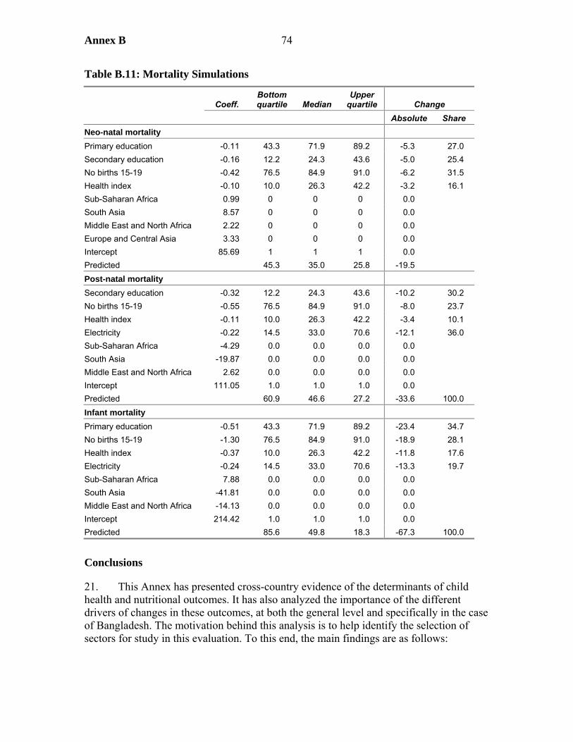
Annex B 74

Table B.11: Mortality Simulations

Coeff. Bottom quartile Median

Upper quartile Change

Absolute Share Neo-natal mortality Primary education -0.11 43.3 71.9 89.2 -5.3 27.0 Secondary education -0.16 12.2 24.3 43.6 -5.0 25.4 No births 15-19 -0.42 76.5 84.9 91.0 -6.2 31.5 Health index -0.10 10.0 26.3 42.2 -3.2 16.1 Sub-Saharan Africa 0.99 0 0 0 0.0 South Asia 8.57 0 0 0 0.0 Middle East and North Africa 2.22 0 0 0 0.0 Europe and Central Asia 3.33 0 0 0 0.0 Intercept 85.69 1 1 1 0.0 Predicted 45.3 35.0 25.8 -19.5 Post-natal mortality Secondary education -0.32 12.2 24.3 43.6 -10.2 30.2 No births 15-19 -0.55 76.5 84.9 91.0 -8.0 23.7 Health index -0.11 10.0 26.3 42.2 -3.4 10.1 Electricity -0.22 14.5 33.0 70.6 -12.1 36.0 Sub-Saharan Africa -4.29 0.0 0.0 0.0 0.0 South Asia -19.87 0.0 0.0 0.0 0.0 Middle East and North Africa 2.62 0.0 0.0 0.0 0.0 Intercept 111.05 1.0 1.0 1.0 0.0 Predicted 60.9 46.6 27.2 -33.6 100.0 Infant mortality Primary education -0.51 43.3 71.9 89.2 -23.4 34.7 No births 15-19 -1.30 76.5 84.9 91.0 -18.9 28.1 Health index -0.37 10.0 26.3 42.2 -11.8 17.6 Electricity -0.24 14.5 33.0 70.6 -13.3 19.7 Sub-Saharan Africa 7.88 0.0 0.0 0.0 0.0 South Asia -41.81 0.0 0.0 0.0 0.0 Middle East and North Africa -14.13 0.0 0.0 0.0 0.0 Intercept 214.42 1.0 1.0 1.0 0.0 Predicted 85.6 49.8 18.3 -67.3 100.0

Conclusions

21. This Annex has presented cross-country evidence of the determinants of child health and nutritional outcomes. It has also analyzed the importance of the different drivers of changes in these outcomes, at both the general level and specifically in the case of Bangladesh. The motivation behind this analysis is to help identify the selection of sectors for study in this evaluation. To this end, the main findings are as follows:

75 Annex B

• While health inputs do matter for child health outcomes, they are by no means the sole – nor always the most important – determinant of these outcomes. It makes good sense to incorporate determinants from other sectors.

• Education emerges as a very robust determinant of child health and nutritional outcomes. The evidence is mixed on whether primary education is sufficient for there to be a beneficial effect, or whether secondary education is required. The quality of education is a factor underlying this distinction. If many children are still illiterate after primary school graduation, then its beneficial effects will be limited.

• Access to media is important for nutrition, presumably reflecting access to health and nutrition information. For mortality, electrification provides a better fit. Although this variable is highly correlated with access to media, electrification may provide additional channels for better health than simply health information.

• Activities in support of economic growth are one way in which external assistance can improve health and nutrition outcomes. However, the evidence suggests that these channels have not been the dominant ones, especially in Bangladesh.

• In summary, these findings support the choice of sectors for this study, that is health and nutrition, female secondary education, and rural electrification.

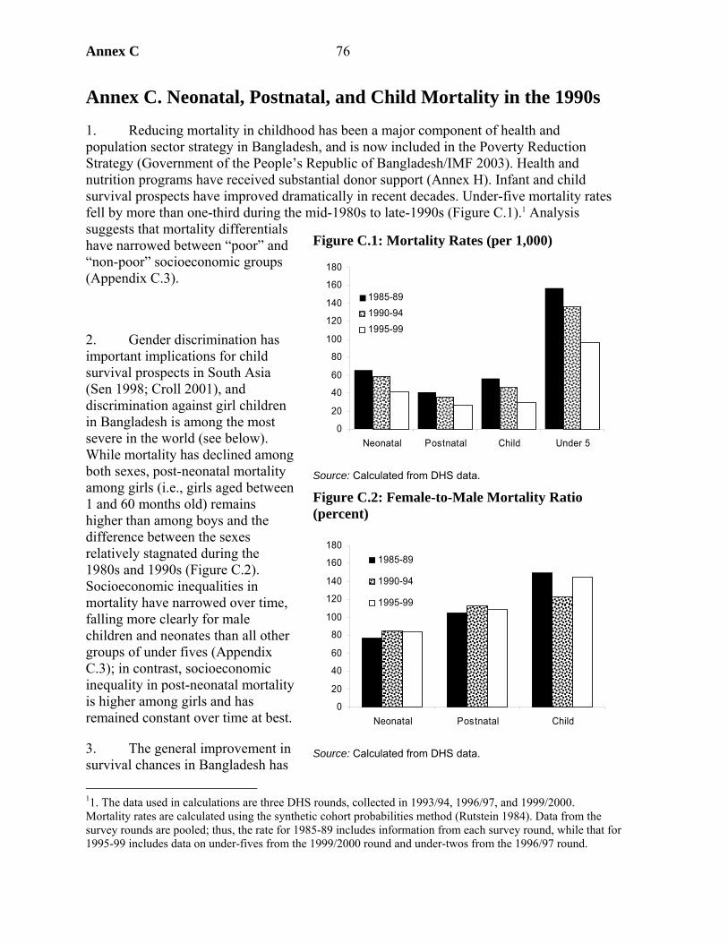
Annex C 76

Annex C. Neonatal, Postnatal, and Child Mortality in the 1990s

1. Reducing mortality in childhood has been a major component of health and population sector strategy in Bangladesh, and is now included in the Poverty Reduction Strategy (Government of the People’s Republic of Bangladesh/IMF 2003). Health and nutrition programs have received substantial donor support (Annex H). Infant and child survival prospects have improved dramatically in recent decades. Under-five mortality rates fell by more than one-third during the mid-1980s to late-1990s (Figure C.1).1 Analysis suggests that mortality differentials have narrowed between “poor” and “non-poor” socioeconomic groups (Appendix C.3).

2. Gender discrimination has important implications for child survival prospects in South Asia (Sen 1998; Croll 2001), and discrimination against girl children in Bangladesh is among the most severe in the world (see below). While mortality has declined among both sexes, post-neonatal mortality among girls (i.e., girls aged between 1 and 60 months old) remains higher than among boys and the difference between the sexes relatively stagnated during the 1980s and 1990s (Figure C.2). Socioeconomic inequalities in mortality have narrowed over time, falling more clearly for male children and neonates than all other groups of under fives (Appendix C.3); in contrast, socioeconomic inequality in post-neonatal mortality is higher among girls and has remained constant over time at best.

3. The general improvement in survival chances in Bangladesh has 11. The data used in calculations are three DHS rounds, collected in 1993/94, 1996/97, and 1999/2000. Mortality rates are calculated using the synthetic cohort probabilities method (Rutstein 1984). Data from the survey rounds are pooled; thus, the rate for 1985-89 includes information from each survey round, while that for 1995-99 includes data on under-fives from the 1999/2000 round and under-twos from the 1996/97 round.

Figure C.1: Mortality Rates (per 1,000)

0

20

40

60

80

100

120

140

160

180

Neonatal Postnatal Child Under 5

1985-891990-941995-99

Source: Calculated from DHS data.

Figure C.2: Female-to-Male Mortality Ratio (percent)

0

20

40

60

80

100

120

140

160

180

Neonatal Postnatal Child

1985-89

1990-94

1995-99

Source: Calculated from DHS data.

Annex C 77

been well documented. Ten years ago, Kabir and Amin (1993, 10) stated that “the fall in infant mortality [since the early 1980s] may be attributed to the large-scale immunization of children from the early 1980s, development of the health infrastructure at the grassroots level and increased awareness of health care issues among the population through the intervention of mass communications channels.” This paper analyzes the determinants of mortality during the 1990s using Demographic and Health Survey (DHS) data, and attempts to ascertain the weight of various factors in achieving the improvement in infant and child survival using decomposition methods.

MODELING CHILDHOOD MORTALITY RISK

4. The usual point of reference for analyzing mortality determinants, at least in the demographic literature, is Mosley and Chen’s (1984) framework, which models mortality outcomes as being determined proximately by factors such as nutrient availability, use of health services, injuries and maternal fertility, which in turn depend on the underlying biological conditions (child-specific), socioeconomic and behavioral conditions (mother or household-specific), and environmental conditions including service provision (community-specific).

5. The economic literature derives from the household’s utility maximization problem. Households have a utility function – determining their preference orderings over consumption of different goods, including child health and nutritional status and leisure – which is maximized subject to the household’s labor constraint and the health and nutrition production functions. The health and nutrition production functions are specified as:

H and N = F(NUTR-1, H-1, INC, MOTHED, CHILD, HCARE, ENV)

6. H and N are, respectively, health and nutritional status produced by each child, which depend on the child’s nutrition and health histories, NUTR-1 and H-1, household income, INC, mother’s education and knowledge, MOTHED, child specific factors, CHILD (such as gender, age, birth order), utilization of health services, HCARE, and factors determining exposure to environmental risk, ENV (e.g., water, sanitation and pollution) (see Chamarbagwala et al. 2004).

7. The economic model is generally consistent with demographic interpretations in terms of identifying determinants of health status. However, it also emphasizes that decisions on health are taken jointly with other household decisions such as labor supply. Thus, current income is considered endogenous to health status, so that its inclusion in multiple regression analysis results in inconsistent parameter estimates. A solution is to use wealth as a proxy for income, as it is unlikely to be endogenous to current nutrition/health choices – thus producing consistent estimates.2 Furthermore, determining the impact of household decision variables – i.e., variables determined in part behaviorally, such as utilization of health care – is problematic because of unobserved heterogeneity. In other words, where heterogeneous household behavioral characteristics cannot be fully accounted for in the set of explanatory variables, they are subsumed into the error term. Hence, if these characteristics are correlated with other explanatory variables, inconsistent estimates result (Rosenzweig and Schultz 2. DHS collects information on household durable goods ownership and housing quality, which can be used to construct a wealth index. DHS does not collect data on income or expenditure.

Annex C 78

1983). Two approaches can be taken to ameliorate this problem. The “health production function” approach estimates proximate determinants of health status using multi-stage estimation where the first-stage equation predicts the behavioral factors for each observation. However, this approach requires identifying instruments exogenous to child health status.3 The alternative is to estimate reduced-form “health demand functions,” linking health outcome to underlying variables affecting behavioral choices, e.g., presence of health and family planning facilities in the community, or distance from that facility.

8. The demand function approach is a popular solution, particularly in analysis of mortality using survival models. However, by not including proximate determinants as explanatory variables, the approach is likely to understate the importance of factors such as health care. Moreover, it is these proximate determinants which are the most interesting for policymakers since they are most amenable to policy intervention. The remainder of this section reviews empirical evidence regarding which variables affect mortality outcomes, drawing on a meta-analysis carried out for this study (Chamarbagwala et al. 2004).

Child-Specific Factors

9. Biological factors are important causes of death in infancy, particularly in the first month of life. Mother’s age is usually found to have a convex (U-shaped) effect on infant mortality. Infants born to mothers under 20 and over 35 are at higher risk of death, because women under 20 are less likely to have fully developed reproductive systems, while the reproductive systems of women over 35 may be deteriorated. The relationship between mother’s age and post-infant survival is due to other factors, for example because children of older women are more likely to be competing with other (younger) siblings; the relationship between mother’s age on child mortality is therefore more likely to be linear, although children of very young mothers may suffer through the lack of maturity of the mother. This is more likely to be a factor when first births occur at a young age, as is the case in Bangladesh.

10. Child’s gender has a strong relationship with survival chances. For biological reasons, males have a higher natural risk of death at all ages. However, it is well known that preference for boys over girls is strong throughout Asia, including Bangladesh (Croll 2001), with discrimination aggravated during crisis periods (see Bairagi 1986). Human interventions override biological factors at later stages in infancy, to the extent that, while neonatal mortality is typically higher among boys, under-five mortality rates are higher among girls. In the multivariate regression studies included in the meta-analysis, the coefficient on female child was insignificant or significantly negative for infant mortality, whereas in studies of child mortality the coefficient was insignificant or significantly positive (Chamarbagwala et al. 2004). The estimated effect of sex on mortality is likely to be conservative due to sex-selective omissions in reported birth histories, which Bairagi et al. (1999) note will artificially lower mortality estimates among girls, although this effect is less in countries where the technology is not widely available.

3. Information on differences in health outcomes and parental behavior within the same family can be used to get around the endogeneity problem, though this method can only be applied to families for which there are two or more live births (Rosenzweig and Schultz 1983).

Annex C 79

11. The relationship between birth order and mortality risk is likely to be convex (U-shaped), reflecting mother’s age, social preferences, and food availability for older children. On the one hand, mortality is usually high among firstborns, particularly in infancy, partly because these births are more likely to occur before the mother has reached physical maturity. On the other hand, high birth order (i.e., being born later than other siblings) is expected to increase mortality risk for two reasons: physiologically, because women who have had many pregnancies are more likely to be physically depleted, and behaviorally, particularly where birth spacing is lower, due to constraints on household resources. However, women who have had more children are likely to be those experiencing higher mortality rates among their offspring. This will lead to spurious correlation between birth order and mortality risk due to unobserved correlations between siblings (frailty effects). It is important to control for this source of heterogeneity in mortality risk across families (see below).

12. Children are at higher risk of mortality when born after short intervals.4, 5 This reflects a number of factors (Koenig et al. 1990):

• Biological factors among prenates (fetal growth harmed by weakened nutritional reserves of the mother, who has been recently pregnant and lactating) and among infants where potential milk production is impaired.

• Socioeconomic and behavioral factors, i.e., competition among post-neonatal siblings for nutrition and mother’s care, where parents’ choices determine which child is favored. Either the younger child is neglected in favor of the older child, or vice versa, so that short subsequent birth interval becomes an important mortality risk factor – e.g., due to a new pregnancy, children are weaned earlier without receiving adequate nutritional substitutes for breast milk. Alternatively, both may be disadvantaged due to limited total family resources.

• Disease, since a higher number of young children in the household means that the likelihood of contracting contagions such as measles is higher.

13. Son preference may also have an indirect effect on girls’ mortality rates when parents choose to reduce birth interval because they are unhappy with the current gender composition of their offspring (ibid.).

4. The positive correlation between preceding birth order and mortality could be spurious due to prematurity. Premature births have higher mortality risk and, by definition, a lower birth interval, so the effect of a regression coefficient on preceding birth interval could simply be picking up the relationship between prematurity and perinatal mortality (Miller 1989). Miller et al. (1992) find that controlling for gestation period reduces the estimated effects of low birth interval by as much as one-third.

5. Subsequent birth interval is also likely to affect mortality risk of children through a number of channels, including premature weaning and reduced quantity and quality of parental resources devoted to the older child in infancy (e.g., because the mother is physically tired and therefore less able to provide adequate care for sick children), and in childhood due to competition among siblings for limited familial resources, if the family believes that he or she has already passed the critical stage for survival (Muhuri and Menken 1997). However, the relation between subsequent birth interval and mortality is likely to be highly endogenous because birth interval is likely to be shorter if the older child has died; this effect operates both behaviorally, where parents choose to replace the lost child, and biologically, as death of the previous infant or young child interrupts breastfeeding causing ovulation to return early (Palloni and Tienda 1986; Koenig et al. 1990).

Annex C 80

14. Miller et al. (1992) find that mortality risk is higher among children born less than 15 months after the preceding child than those born more than 15 months after or those who are firstborns, reflecting the likelihood that, for birth intervals less than 15 months, conception occurred before the preceding child was 6 months old, therefore increasing chances that the child would have been weaned early.6 The meta-analysis found that short preceding birth interval increases infant mortality risk, while short subsequent birth interval increases child mortality risk (Chamarbagwala et al. 2004).

15. The effects of birth interval, gender, and birth order are interlinked. In particular, in South Asia, mortality risks are likely to be high among girls who have one or more older sisters (Muhuri and Preston 1991; Muhuri and Menken 1997; Masset and White 2003) or among girls with no male siblings (Croll 2001).7 Some important interactions to consider are between birth order and sex, and between sex of index child and sex composition of older siblings (Masset and White 2003).8

16. Birth order and birth interval are proxies for fertility, so these relationships between birth order, birth interval, and mortality risk indicate that lower fertility means lower mortality. Although birth order and interval have the direct effects described above, they are also picking up the simultaneous relationship between declining fertility and mortality which occurs as the demographic transition proceeds and parents decide to invest in child quality rather than quantity. There will therefore be relationships between these variables and those such as use of health services for the child.

Community-Level Factors

17. Access to decent health care is an important determinant of infant and child survival. Babies delivered in modern health facilities by trained health professionals will have lower risks of death, since presence of a health professional reduces the mortality risk associated with complications during and after labor, while hygienic conditions reduce risk of infection of mother and child. However, where home delivery is the norm, it can be the case that only complicated deliveries take place in health facilities, thus giving a perverse relationship. Immunization should prevent exposure to major killers such as measles, lowering risk of death among children immunized as well as having positive external effects for child survival among the non-immunized in a given community. The meta-analysis of Chamarbagwala et al. (2004) indicates that these factors are indeed significantly correlated with mortality in multivariate studies.

6. It is possible to test between the competing explanations of why preceding birth interval affects mortality by interacting preceding birth interval with mortality status of the previous child, with a significant negative effect on the interaction term providing support for the resource competition theory (Bairagi et al. 1999).

7. Muhuri and Preston (1991) argue that mortality risk is likely to be greater for both (younger) boys and girls the greater the number of (older) siblings of the same sex there are, since children of the same sex are better substitutes for one another in the family economy than children of the opposite sex (though the effect for girls will be higher).

8. Regarding the latter, it is important to use sibling sex composition at birth of the index child, as opposed to sex composition of siblings at interview date, since the latter will be endogenous to mortality.

Annex C 81

18. Sanitary toilet facilities and safe drinking water improve survival chances by reducing exposure to diseases such as diarrhea. While it can be reasoned that water and sanitation are more likely to have greater effects as children get older and start using the services directly, Chamarbagwala et al. (2004) show that, in fact, differentials in water and sanitation variables are more likely to be significant determinants of infant mortality in multivariate studies.

19. Electrification is usually found to have a positive impact on infant survival, but an insignificant impact on child survival (Chamarbagwala et al. 2004). The channels through which access to electricity affects mortality are, however, contentious, though possible candidates are that electrification facilitates use of modern medicine in health facilities (e.g., a refrigerator allows hygienic storage of vaccines), improves transfer of health information (through television and radio), and improves domestic air quality. Electrification is, of course, highly correlated with locality (particularly rural versus urban) and it is also likely that electrification expansion favors less remote and better off communities (which are able to pay for the services), raising issues of reverse causality at community level. Controlling for socioeconomic status, broadly, should account for this.

20. Water, sanitation, electricity, and health services are labeled as community-level variables, because communities gain access to them at the same time (e.g., due to electrification programs, construction of a health center, etc.) and because it is recognized that there are strong positive externalities from improved services, e.g., in terms of disease control (the degree of coverage in the community has an important effect on reducing morbidity and mortality among the community). However, where intra-community variation occurs due to variation in household income and preferences and where externalities do not exist, “community level” may be an erroneous classification. This is likely to be particularly true for aspects of health care such as antenatal care, where access is determined at the community level by presence of a nearby health facility, but whether parents seek professional health care is determined at family level by such factors as income and maternal education and preferences.

21. Most multivariate analyses control for physical locality (region and rural/urban sector), to represent unobserved determinants of mortality risk, mainly in terms of access to health care and clean water and sanitation, and possibly geographic socio-cultural factors. Chamarbagwala et al. (2004) showed that urban location is frequently related to significantly lower mortality risk in multivariate models.

Household-Level Socioeconomic Factors9

22. Socioeconomic status determines nutrition, illness, and ability to access health care. Household socioeconomic status represents direct determinants of mortality such as nutrient intake and likelihood of affording health treatment. Multivariate studies generally find

9. Household size and age composition are potentially important determinants of child health status, both indirectly as a measure of the ratio of hands to mouths available, but also directly by indicating the quantity and quality of care a given child may be able to receive (Chamarbagwala et al. 2004). However, most studies, including this one, are unable to include directly indicators of household size to explain fertility and mortality differentials because household composition is endogenous to fertility decisions and mortality.

Annex C 82

income or wealth to have a significantly positive impact on child survival, though no impact on infant survival prospects (Chamarbagwala et al. 2004).

23. Education of household members is often used to proxy socioeconomic status as an indicator of potential earnings capacity of the labor force. In analyses of child health, however, there is a clear distinction between mother’s and father’s education. Whereas father’s education may affect child health indirectly through socioeconomic status, mother’s education has clear direct links to children for a number of reasons. Education can proxy for basic knowledge about nutrition and child care, including knowledge of good caring practices, health problems and treatment, and the importance of immunization and techniques such as use of oral rehydration salts (ORS) to treat diarrhea. Educated mothers are more likely to seek treatment from health professionals, and see this as their right. Moreover, educated mothers may also have greater decision-making ability within their families and, therefore, greater say on child nutrition and health decisions (Caldwell 1979). Chamarbagwala et al. (2004) find that parental, particularly maternal, education has a positive effect on infant and child survival in studies of mortality.

24. In a highly patriarchal society such as Bangladesh, marriage disruption caused by divorce, separation, or abandonment is potentially disastrous for women and therefore children. Where women have no support network, or are disowned by their families, they will be highly vulnerable and may have to remarry, or accept a new husband they know is already married. In such cases, the children may not fare better if they are not welcome to the new husband’s family. The effect of divorce is likely to be greater for infants because young children suffer more from reduced quantity and quality of mother’s care, e.g., because she is working to support the family (Bhuiya and Chowdhury 1997).

Unobserved Factors

25. Unobserved factors determining mortality among families include genetic or other family-specific practices altering childhood survival prospects and are referred to in the literature as “frailty” effects. As noted above, it is important to account for sources of unobserved heterogeneity in empirical estimation, since correlation between observations can lead to inconsistent and inefficient statistical estimates, as demonstrated for survival models by Heckman and Singer (1984). Statistical tools can be used to account for frailty, e.g., by assuming that observations at child level are correlated among mothers; however, when modeling frailty among siblings, it is also important to control for the death of the preceding child separately, since the association between immediate pairs of siblings may be stronger (Zenger 1993).

DATA AND METHODOLOGY

26. Data used for modeling mortality in Bangladesh come from the nationally representative Demographic and Health Survey. DHS collects data on complete fertility histories of all ever-married women aged 10-49, as well as data on health status and health care, contraception, women’s knowledge, beliefs and caring practices, household composition, and other socioeconomic factors such as water and sanitation facilities,

Annex C 83

household asset ownership, and educational attainment. Data were collected over three rounds during the 1990s: 1993/94, 1996/97, and 1999/2000.

27. Most empirical studies analyze mortality determinants for infants (up to one year old) and children (between one and approximately five years old) separately. Biological and environmental factors should be more important for infants, while socioeconomic and behavioral factors become more important as children get older, though some behavioral factors, such as delivery assistance and antenatal care, are also important for neonatal survival prospects.10 It is also useful to divide infant mortality further into neonatal (first month after birth) and postnatal (second to twelfth months). Appendix C.1 summarizes results of other multivariate studies examining childhood mortality in Bangladesh.

28. The major econometric issue with mortality analysis is that survey data are right-censored: survival status of children born within the period of analysis is unknown past the survey date. This introduces a bias in conventional regression estimates, such as those obtained from probit/logit regression, unless observations are omitted for children born within x time periods before the survey, where x is the mortality rate being analyzed. Survival analysis, by accounting for right-censoring, enables all observations to be included and is therefore statistically more efficient.

29. A frequently used model of mortality is the Cox proportional hazards model.11 The model assumes that the risk of death for any age can be calculated by adjusting the baseline risk for that age by an exponential set of factors. The model can be summarized as follows:

hi(t) = h0(t)exp(βxi)

where hi(t) represents the hazard (mortality) rate at time (t) for individual i and h0(t) is the age-specific baseline hazard, which is the mortality risk at each age in the case where all explanatory variables are equal to zero (i.e., equivalent to the constant term in a standard linear regression); xi is the matrix of covariates and β the estimated parameters. Child mortality is modeled using the proportional hazards specification. For neonates and postnates, however, it is reasonable to drop observations on, respectively, children born in the month of the interview and children born in the year before the interview and estimate using a probit model. The probit model is summarized as:

P(yi=1) = Φ(βxi)

10. Note that some variables indicate different underlying cause for different age groups. Males have higher biological mortality risk than females at all ages, which is reflected in higher observed mortality rates among male neonates; higher observed mortality rates among girl children in South Asia, on the other hand, is entirely behavioral, due to son preference. Similarly, short birth interval and higher birth order are known to increase mortality risk in (neonatal) infancy, possibly for biological reasons such as physical depletion of the mother, but for older children effects will be entirely behavioral, and probably modified by sex of the child.

11. The advantage of the Cox semi-parametric estimator is that, in comparison to fully parametric proportional hazards models such as the Weibull, assumptions do not have to be made about the baseline hazard.

Annex C 84

where P(yi=1) is the probability of the event occurring for individual i, in the case of neonatal death in the first month after birth or for postnates between the second and twelfth months following birth, and Φ is the standard normal cumulative density.

30. A determinant can alter risk of death through two routes: where the effect of the factor changes over time (i.e., changes in the coefficient estimate); and where the distribution of the factor changes among the population (i.e., changes in the mean of the variable). A decomposition analysis is undertaken following model estimation in order to determine the latter.

31. As noted above, there are likely to be issues of unobserved heterogeneity of important proximate causes of health status relating to behavioral choices which will cause biased estimation of the “true” (technological) impact of the explanatory variables on health outcomes. Behavioral factors, such whether the mother seeks antenatal care during pregnancy and delivery assistance, are likely to be endogenous to health status – i.e., she seeks health care during pregnancy because she is experiencing complications or previously experienced complications during birth, which are likely to be correlated among her children due to frailty. On the other hand, immunization is likely to be less endogenous than antenatal care, since it is preventative rather than curative.12 But even where reverse causality is not likely to be a serious issue, unobserved heterogeneity in preferences will lead to erroneous estimates of the effect of decision variables, particularly those relating to caring practices. Some sources of heterogeneity can be controlled for with other explanatory variables – for example, maternal education and indicators of knowledge of modern health care practices. In addition, modeling frailty should account for some of the unobserved heterogeneity (though it is unable to account for the likelihood of behavior changing from birth to birth as it is assumed that frailty is constant across births for the same mother).

32. It is particularly likely that antenatal visits and delivery assistance are endogenous to child health, both because of reverse causality and unobserved heterogeneity with respect to mothers’ behavioral choices. Under these conditions, consistency requires use of instrumental variables. Greene (1998; see also Greene 2000: 849) indicates that an endogenous system of limited dependent variable equations can be appropriately modeled as a multivariate probit model. Suppressing individual subscripts, the trivariate model can be expressed as:

P(y1=1, y2=1, y3=1) = Φ3(β1x1 + γy2 + δy3, β2x2, β3x3, ρ21, ρ31, ρ32).

Φ3 indicates the trivariate standard normal density; y1, y2, and y3 are, respectively, the probabilities of dying, receiving antenatal care, and delivery assistance; the equation estimating probability of dying includes antenatal care in the explanatory variables set, where γ and δ are the estimated parameters on antenatal visits and assisted delivery; β2x2 and β3x3 are the vectors of estimated coefficients and explanatory variables of the equations for antenatal visits and assisted delivery; ρ represents the estimated correlation between error terms of each equation – their statistical significance, therefore, provide evidence for endogeneity. Identifying

12. For immunization of children, the variable used in this paper is the geographical mean (by cluster and gender) of children immunized. This is because immunization data are only collected on children who are alive at the time of interview, so immunization status cannot be used. The same procedure is used for Vitamin A supplementation, which is also only available for live children.

Annex C 85

instruments used in the equations for antenatal visits and delivery assistance are presence of health and information facilities in the community, distances from Upazilla and District headquarters; in addition, the equation for antenatal visits includes the non-self geographical area mean (by maternal education attainment and sex of child) of the dependent variable.

ESTIMATION RESULTS

33. The estimation strategy is to pool data for the three survey rounds and distinguish between two periods, the late-1980s-early-1990s and the mid-late 1990s. Due to the likelihood that the relationships between some covariates and mortality change during early childhood, separate regressions are estimated for neonatal mortality (less than 1 completed month), postnatal mortality (from 1 to 11 completed months), and child mortality (from 12 to 59 months).

34. Table C.1 presents bivariate estimates of mortality rates by various factors. Mortality rates are lower among wealthier households, though there is little difference between mortality rates among the bottom four quintiles. Mortality is higher in households with no electricity, poor sanitation, and non-piped (direct into the home) drinking water. The Divisions of Chittagong13 and Barisal have the highest mortality rates while Khulna has the lowest; girls fare worst in Chittagong. Mortality rates are lower among children whose mothers have formal education, especially when they have at least upper secondary education (grade 10 onwards), are not divorced or remarried, and are more mobile (can go out and/or can go to the health center). Child-specific characteristics associated with higher mortality risk include multiple birth, short preceding birth interval (less than 15 months), and death of previous child. Higher mortality rates are experienced by boys in the neonatal period, but by girls in the post-neonatal period. Children whose mothers received antenatal care, two or more tetanus toxoid (TT) vaccinations or who have been breastfed, have better survival chances.14 Mortality rates are lower among children living in communities where over half of the children have received at least one vaccination or received Vitamin A in the preceding six months. Babies delivered by a doctor have higher neonatal mortality rates than those delivered by nurses or traditional birth attendants (TBAs), suggesting that doctor-assisted births are more likely to occur for high-risk cases.

Table C.1: Mortality Rates by Selected Characteristics

Neonatal mortality rate

(standard error) Infant mortality rate

(standard error) Child mortality rate

(standard error) All children 0.047 (0.002) 0.077 (0.002) 0.033 (0.001) Characteristics of household Wealth quintile 1 0.054 (0.004) 0.095 (0.005) 0.051 (0.004) Wealth quintile 2 0.050 (0.004) 0.085 (0.005) 0.044 (0.004) Wealth quintile 3 0.050 (0.004) 0.078 (0.005) 0.031 (0.003) Wealth quintile 4 0.049 (0.004) 0.075 (0.004) 0.027 (0.003) Wealth quintile 5 0.034 (0.003) 0.054 (0.004) 0.017 (0.002) No electricity 0.052 (0.002) 0.084 (0.002) 0.037 (0.002)

13. Chittagong includes Sylhet, which became a separate Division in 1996/97.

14. Due to extreme endogeneity of breastfeeding with respect to child health status – e.g., low birth weight or sick children may be unable to breastfeed – variables indicating breastfeeding are omitted from the explanatory variable set in multivariate analysis.

Annex C 86





(standard error) Electricity 0.034 (0.003) 0.057 (0.004) 0.021 (0.002) Unsanitary toilet 0.052 (0.002) 0.083 (0.003) 0.038 (0.002) Sanitary toilet 0.038 (0.003) 0.063 (0.003) 0.022 (0.002) Non-piped water 0.048 (0.002) 0.078 (0.002) 0.033 (0.001) Piped water 0.030 (0.007) 0.049 (0.009) 0.016 (0.005) Characteristics of mother Mother not attended school 0.052 (0.002) 0.088 (0.003) 0.042 (0.002) Mother attended some primary 0.048 (0.004) 0.079 (0.005) 0.029 (0.003) Mother finished primary 0.039 (0.005) 0.065 (0.006) 0.022 (0.004) Mother attended lower secondary 0.042 (0.004) 0.054 (0.004) 0.010 (0.003) Mother attended upper secondary or higher 0.014 (0.005) 0.019 (0.006) 0.003 (0.001) Mother married 0.047 (0.002) 0.077 (0.002) 0.032 (0.001) Mother divorced 0.061 (0.014) 0.113 (0.019) 0.047 (0.011) Mother married once 0.047 (0.002) 0.076 (0.002) 0.032 (0.001) Mother remarried 0.047 (0.006) 0.095 (0.009) 0.048 (0.007) Mobility index=0 0.059 (0.004) 0.095 (0.005) 0.036 (0.005) Mobility index=1 0.048 (0.002) 0.077 (0.003) 0.034 (0.002) Mobility index=2 0.037 (0.003) 0.064(0.004) 0.028(0.003) Characteristics of child Child male 0.053 (0.002) 0.081(0.003) 0.029(0.002) Child female 0.042 (0.002) 0.073(0.003) 0.037(0.002) Single birth 0.044 (0.002) 0.072 (0.002) 0.032 (0.001) Multiple birth 0.261 (0.025) 0.404 (0.028) 0.105 (0.025) Previous interval >15 0.045 (0.002) 0.074 (0.002) 0.031 (0.001) Previous interval <15 0.099 (0.011) 0.171 (0.014) 0.064 (0.009) Previous child survived 0.046 (0.002) 0.074 (0.002) 0.031 (0.001) Previous child died 0.063 (0.006) 0.102 (0.007) 0.048 (0.005) First-born child 0.069 (0.004) 0.099 (0.004) 0.023 (0.002) Second or third birth order 0.038 (0.002) 0.063 (0.003) 0.033 (0.002) Fourth or fifth birth order 0.037 (0.003) 0.067 (0.004) 0.038 (0.003) Sixth or higher birth order 0.044 (0.004) 0.089 (0.006) 0.041 (0.004) Rural*Born Dec-Jan 0.052 (0.004) 0.078 (0.005) 0.031 (0.003) Rural*Born Feb-Mar 0.048 (0.004) 0.074 (0.005) 0.039 (0.004) Rural*Born Apr-May 0.039 (0.004) 0.067 (0.006) 0.044 (0.005) Rural*Born Jun-Jul 0.050 (0.005) 0.083 (0.006) 0.039 (0.005) Rural*Born Aug-Sep 0.049 (0.004) 0.079 (0.006) 0.034 (0.004) Rural*Born Oct-Nov 0.053 (0.004) 0.091 (0.005) 0.030 (0.003) Delivered by doctor 0.051 (0.007) 0.069 (0.008) 0.008 (0.005) Delivered by nurse 0.034 (0.006) 0.068 (0.009) 0.017 (0.008) Delivered by trained TBA 0.043 (0.006) 0.067 (0.007) 0.034 (0.011) Delivered by untrained TBA 0.045 (0.002) 0.072 (0.003) 0.030 (0.003) Delivered by other 0.053 (0.003) 0.089 (0.004) 0.034 (0.002) Not breastfed 0.686 (0.014) 0.766 (0.014) 0.074 (0.022) Breastfed 0.003 (0.000) 0.029 (0.001) 0.026 (0.002) No antenatal visits 0.051 (0.002) 0.084 (0.003) 0.035 (0.002) Some antenatal visits 0.036 (0.003) 0.058 (0.004) 0.019 (0.003) Less than 2 TT vaccinations 0.056 (0.002) 0.092 (0.003) 0.035 (0.002) 2 or more TT vaccinations 0.039 (0.002) 0.064 (0.003) 0.023 (0.003) Characteristics of community Located in Barisal 0.047 (0.005) 0.083 (0.007) 0.038 (0.005) Located in Chittagong 0.049 (0.003) 0.082 (0.004) 0.042 (0.003) Located in Dhaka 0.046 (0.003) 0.081 (0.004) 0.035 (0.003) Located in Khulna 0.043 (0.004) 0.060 (0.005) 0.014 (0.003) Located in Rajshahi 0.049 (0.003) 0.074 (0.004) 0.026 (0.003) Female child*located in Barisal 0.031 (0.006) 0.069 (0.009) 0.034 (0.007) Female child*located in Chittagong 0.045 (0.004) 0.079 (0.005) 0.050 (0.004) Female child*located in Dhaka 0.041 (0.004) 0.076 (0.005) 0.038 (0.004) Female child*located in Khulna 0.041 (0.006) 0.060 (0.007) 0.012 (0.003) Female child*located in Rajshahi 0.044 (0.005) 0.070 (0.006) 0.032 (0.004)

Annex C 87





(standard error) Less than half of children in community received Vitamin A supplement 0.049 (0.002) 0.081 (0.002) 0.035 (0.002) More than half of children received Vitamin A supplement 0.039 (0.033) 0.059 (0.004) 0.021 (0.003) Less than half of children in community vaccinated 0.052 (0.004) 0.088 (0.005) 0.053 (0.006) More than half of children in community vaccinated 0.046 (0.002) 0.075 (0.002) 0.030 (0.001)

Neonatal Mortality

35. Table C.2 presents estimates of the probit analysis of neonatal mortality. The table reports coefficient estimates, as well as marginal effects (dF/dX), which indicate the effect of a unit change in the explanatory variable on the probability of death. The regressions bear out the prior expectation that biological characteristics and inadequate access to public services are key factors impeding neonatal survival prospects.

36. Biological factors associated with higher neonatal mortality are gender (male), multiple birth, short preceding birth interval, death of previous sibling, and very low or very high birth order (the estimated turning point is between birth order 6 and 7).15 Mother’s age has a convex effect on mortality risk, the coefficients suggesting that the mother’s optimal age for childbirth is during her late 20s. While these factors are likely to reflect biological characteristics, the significantly negative coefficient on the interaction between death of previous child and birth interval, suggests that newborns are less likely to die when there are fewer children competing for resources.

37. Maternal characteristics are important determinants of neonatal mortality. Newborns have better survival chances if their mothers are more mobile (able to go out to the health center). Mother’s schooling has a negative effect on neonatal mortality, particularly upper secondary (grades 10 through 12) and higher education, as compared to the reference category of no schooling; mothers who have primary education also have fewer neonatal fatalities, though the estimate is imprecise.16 It is possible to examine some of the channels through which education lowers child mortality.17 Specification (2) includes a variable indicating number of modern contraceptive methods known by the mother – a proxy for general knowledge of modern health and child care practices – which is highly significantly negative; schooling remains significant (though its estimated impact is marginally reduced). This suggests that the impact of maternal formal schooling on neonate health operates outside knowledge, though it is possible that maternal education is approximating household socioeconomic status, if the wealth index measures this inaccurately. Indicators of paternal 15. The non-linear variable x enters the probit equation in the form Φ(b1x + b2x2 + …) where … indicates the remaining arguments of the equation. Taking the partial differential with respect to x, setting equal to zero and solving for x gives the maximum/minimum at x = -b1/(2b2).

16. The effect of education is stronger when mothers have completed primary education than when they have not (results not reported).

17. It was also possible to test the impact of education via (self-reported) literacy, though coefficients on the literacy variable were insignificant in all regressions for all three age periods.

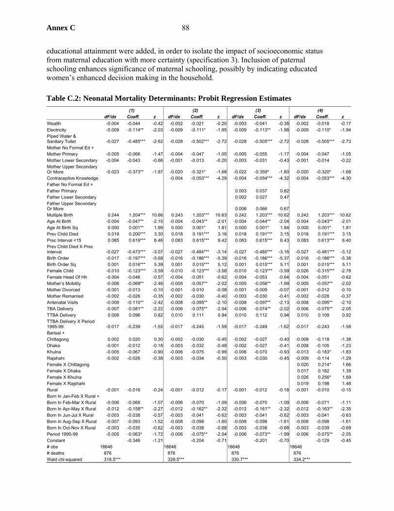
Annex C 88

educational attainment were added, in order to isolate the impact of socioeconomic status from maternal education with more certainty (specification 3). Inclusion of paternal schooling enhances significance of maternal schooling, possibly by indicating educated women’s enhanced decision making in the household.

Table C.2: Neonatal Mortality Determinants: Probit Regression Estimates (1) (2) (3) (4) dF/dx Coeff. z dF/dx Coeff. z dF/dx Coeff. z dF/dx Coeff. z Wealth -0.004 -0.044 -0.42 -0.002 -0.021 -0.20 -0.003 -0.041 -0.38 -0.002 -0.018 -0.17Electricity -0.009 -0.114** -2.03 -0.009 -0.111* -1.95 -0.009 -0.113** -1.98 -0.009 -0.110* -1.94Piped Water & Sanitary Toilet -0.027 -0.485*** -2.62 -0.028 -0.502*** -2.72 -0.028 -0.505*** -2.72 -0.028 -0.505*** -2.73Mother No Formal Ed + Mother Primary -0.005 -0.066 -1.47 -0.004 -0.047 -1.05 -0.005 -0.055 -1.17 -0.004 -0.047 -1.05Mother Lower Secondary -0.004 -0.043 -0.66 -0.001 -0.013 -0.20 -0.003 -0.031 -0.43 -0.001 -0.014 -0.22Mother Upper Secondary Or More -0.023 -0.373** -1.97 -0.020 -0.321* -1.68 -0.022 -0.359* -1.80 -0.020 -0.320* -1.68Contraceptive Knowledge -0.004 -0.053*** -4.29 -0.004 -0.054*** -4.32 -0.004 -0.053*** -4.30Father No Formal Ed + Father Primary 0.003 0.037 0.82 Father Lower Secondary 0.002 0.027 0.47 Father Upper Secondary Or More 0.006 0.066 0.67 Multiple Birth 0.244 1.204*** 10.66 0.243 1.203*** 10.63 0.242 1.203*** 10.62 0.242 1.203*** 10.62Age At Birth -0.004 -0.047** -2.15 -0.004 -0.043** -2.01 -0.004 -0.044** -2.04 -0.004 -0.043** -2.01Age At Birth Sq 0.000 0.001** 1.99 0.000 0.001* 1.81 0.000 0.001* 1.84 0.000 0.001* 1.81Prev Child Died 0.019 0.200*** 3.30 0.018 0.191*** 3.16 0.018 0.191*** 3.15 0.018 0.191*** 3.15Prec Interval <15 0.085 0.619*** 6.46 0.083 0.615*** 6.42 0.083 0.615*** 6.43 0.083 0.613*** 6.40Prev Child Died X Prec Interval -0.027 -0.473*** -3.07 -0.027 -0.484*** -3.14 -0.027 -0.485*** -3.16 -0.027 -0.481*** -3.12Birth Order -0.017 -0.197*** -5.68 -0.016 -0.186*** -5.39 -0.016 -0.186*** -5.37 -0.016 -0.186*** -5.38Birth Order Sq 0.001 0.016*** 5.39 0.001 0.015*** 5.12 0.001 0.015*** 5.11 0.001 0.015*** 5.11Female Child -0.010 -0.123*** -3.59 -0.010 -0.123*** -3.58 -0.010 -0.123*** -3.59 -0.026 -0.315*** -2.78Female Head Of Hh -0.004 -0.046 -0.57 -0.004 -0.051 -0.62 -0.004 -0.053 -0.64 -0.004 -0.051 -0.62Mother’s Mobility -0.006 -0.069** -2.46 -0.005 -0.057** -2.02 -0.005 -0.056** -1.99 -0.005 -0.057** -2.02Mother Divorced -0.001 -0.013 -0.10 -0.001 -0.010 -0.08 -0.001 -0.009 -0.07 -0.001 -0.012 -0.10Mother Remarried -0.002 -0.026 -0.35 -0.002 -0.030 -0.40 -0.003 -0.030 -0.41 -0.002 -0.028 -0.37Antenatal Visits -0.009 -0.110** -2.42 -0.008 -0.095** -2.10 -0.008 -0.097** -2.13 -0.008 -0.095** -2.10TBA Delivery -0.007 -0.081** -2.22 -0.006 -0.075** -2.04 -0.006 -0.074** -2.02 -0.006 -0.075** -2.05TTBA Delivery 0.009 0.096 0.82 0.010 0.111 0.94 0.010 0.112 0.94 0.010 0.109 0.92TTBA Delivery X Period 1995-99 -0.017 -0.239 -1.55 -0.017 -0.245 -1.59 -0.017 -0.249 -1.62 -0.017 -0.243 -1.58Barisal + Chittagong 0.002 0.020 0.30 -0.002 -0.030 -0.45 -0.002 -0.027 -0.40 -0.009 -0.118 -1.38Dhaka -0.001 -0.012 -0.18 -0.003 -0.032 -0.48 -0.002 -0.027 -0.41 -0.008 -0.105 -1.23Khulna -0.005 -0.067 -0.90 -0.006 -0.075 -0.99 -0.006 -0.070 -0.93 -0.013 -0.183* -1.83Rajshahi -0.002 -0.026 -0.38 -0.003 -0.034 -0.50 -0.003 -0.030 -0.45 -0.009 -0.114 -1.29Female X Chittagong 0.020 0.214* 1.66Female X Dhaka 0.017 0.182 1.39Female X Khulna 0.026 0.256* 1.69Female X Rajshahi 0.019 0.198 1.48Rural -0.001 -0.016 -0.24 -0.001 -0.012 -0.17 -0.001 -0.012 -0.18 -0.001 -0.010 -0.15Born In Jan-Feb X Rural + Born In Feb-Mar X Rural -0.006 -0.068 -1.07 -0.006 -0.070 -1.09 -0.006 -0.070 -1.09 -0.006 -0.071 -1.11Born In Apr-May X Rural -0.012 -0.158** -2.27 -0.012 -0.162** -2.32 -0.012 -0.161** -2.32 -0.012 -0.163** -2.35Born In Jun-Jul X Rural -0.003 -0.038 -0.57 -0.003 -0.041 -0.62 -0.003 -0.041 -0.62 -0.003 -0.041 -0.63Born In Aug-Sep X Rural -0.007 -0.093 -1.52 -0.008 -0.098 -1.60 -0.008 -0.098 -1.61 -0.008 -0.098 -1.61Born In Oct-Nov X Rural -0.003 -0.035 -0.62 -0.003 -0.038 -0.68 -0.003 -0.038 -0.68 -0.003 -0.039 -0.69Period 1995-99 -0.005 -0.063* -1.72 -0.006 -0.075** -2.04 -0.006 -0.073** -1.99 -0.006 -0.075** -2.05Constant -0.346 -1.21 -0.204 -0.71 -0.201 -0.70 -0.129 -0.45# obs 18646 18646 18646 18646 # deaths 876 876 876 876 Wald chi-squared 318.5*** 329.5*** 330.7*** 334.2***

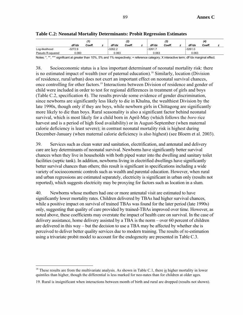
Annex C 89

Table C.2: Neonatal Mortality Determinants: Probit Regression Estimates (1) (2) (3) (4) dF/dx Coeff. z dF/dx Coeff. z dF/dx Coeff. z dF/dx Coeff. z Log-likelihood -3272.9 -3262.2 -3261.7 -3261.0 Pseudo R-squared 0.060 0.063 0.063 0.063 Notes: *, **, *** significant at greater than 10%, 5% and 1% respectively; + reference category; X interactive term; dF/dx marginal effect.

38. Socioeconomic status is a less important determinant of neonatal mortality risk: there is no estimated impact of wealth (nor of paternal education).18 Similarly, location (Division of residence, rural/urban) does not exert an important effect on neonatal survival chances, once controlling for other factors.19 Interactions between Division of residence and gender of child were included in order to test for regional differences in treatment of girls and boys (Table C.2, specification 4). The results provide some evidence of gender discrimination, since newborns are significantly less likely to die in Khulna, the wealthiest Division by the late 1990s, though only if they are boys, while newborn girls in Chittagong are significantly more likely to die than boys. Rural seasonality is also a significant factor behind neonatal survival, which is most likely for a child born in April-May (which follows the boro rice harvest and is a period of high food availability) or in August-September (when maternal calorie deficiency is least severe); in contrast neonatal mortality risk is highest during December-January (when maternal calorie deficiency is also highest) (see Bloem et al. 2003).

39. Services such as clean water and sanitation, electrification, and antenatal and delivery care are key determinants of neonatal survival. Newborns have significantly better survival chances when they live in households with both piped water into the dwelling and sanitary toilet facilities (septic tank). In addition, newborns living in electrified dwellings have significantly better survival chances than others; this result is significant in specifications including a wide variety of socioeconomic controls such as wealth and parental education. However, when rural and urban regressions are estimated separately, electricity is significant in urban only (results not reported), which suggests electricity may be proxying for factors such as location in a slum.

40. Newborns whose mothers had one or more antenatal visit are estimated to have significantly lower mortality rates. Children delivered by TBAs had higher survival chances, while a positive impact on survival of trained TBAs was found for the later period (late 1990s) only, suggesting that quality of care provided by trained-TBAs improved over time. However, as noted above, these coefficients may overstate the impact of health care on survival. In the case of delivery assistance, home delivery assisted by a TBA is the norm – over 60 percent of children are delivered in this way – but the decision to use a TBA may be affected by whether she is perceived to deliver better quality services due to modern training. The results of re-estimation using a trivariate probit model to account for the endogeneity are presented in Table C.3.

18 These results are from the multivariate analysis. As shown in Table C.1, there is higher mortality in lower quintiles than higher, though the differential is less marked for neo-nates than for children at older ages.

19. Rural is insignificant when interactions between month of birth and rural are dropped (results not shown).

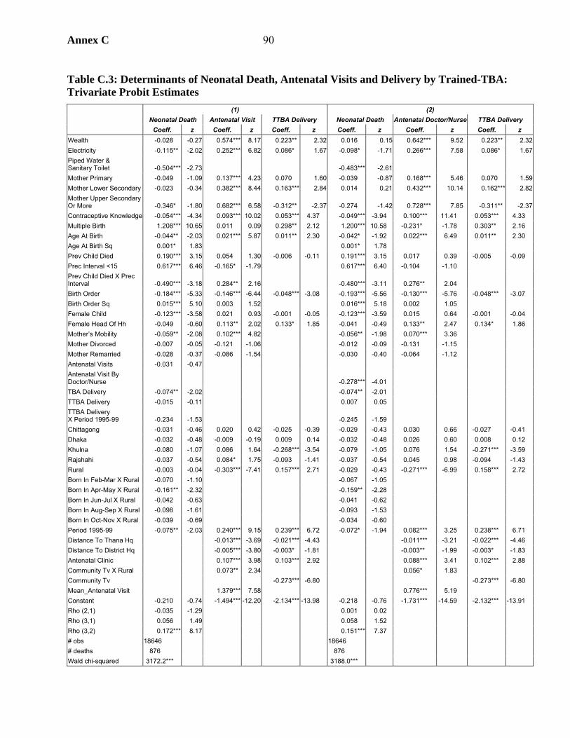
Annex C 90

Table C.3: Determinants of Neonatal Death, Antenatal Visits and Delivery by Trained-TBA: Trivariate Probit Estimates

(1) (2) Neonatal Death Antenatal Visit TTBA Delivery Neonatal Death Antenatal Doctor/Nurse TTBA Delivery Coeff. z Coeff. z Coeff. z Coeff. z Coeff. z Coeff. z

Wealth -0.028 -0.27 0.574*** 8.17 0.223** 2.32 0.016 0.15 0.642*** 9.52 0.223** 2.32Electricity -0.115** -2.02 0.252*** 6.82 0.086* 1.67 -0.098* -1.71 0.266*** 7.58 0.086* 1.67Piped Water & Sanitary Toilet -0.504*** -2.73 -0.483*** -2.61 Mother Primary -0.049 -1.09 0.137*** 4.23 0.070 1.60 -0.039 -0.87 0.168*** 5.46 0.070 1.59Mother Lower Secondary -0.023 -0.34 0.382*** 8.44 0.163*** 2.84 0.014 0.21 0.432*** 10.14 0.162*** 2.82Mother Upper Secondary Or More -0.346* -1.80 0.682*** 6.58 -0.312** -2.37 -0.274 -1.42 0.728*** 7.85 -0.311** -2.37Contraceptive Knowledge -0.054*** -4.34 0.093*** 10.02 0.053*** 4.37 -0.049*** -3.94 0.100*** 11.41 0.053*** 4.33 Multiple Birth 1.208*** 10.65 0.011 0.09 0.298** 2.12 1.200*** 10.58 -0.231* -1.78 0.303** 2.16 Age At Birth -0.044** -2.03 0.021*** 5.87 0.011** 2.30 -0.042* -1.92 0.022*** 6.49 0.011** 2.30 Age At Birth Sq 0.001* 1.83 0.001* 1.78 Prev Child Died 0.190*** 3.15 0.054 1.30 -0.006 -0.11 0.191*** 3.15 0.017 0.39 -0.005 -0.09 Prec Interval <15 0.617*** 6.46 -0.165* -1.79 0.617*** 6.40 -0.104 -1.10 Prev Child Died X Prec Interval -0.490*** -3.18 0.284** 2.16 -0.480*** -3.11 0.276** 2.04 Birth Order -0.184*** -5.33 -0.146*** -6.44 -0.048*** -3.08 -0.193*** -5.56 -0.130*** -5.76 -0.048*** -3.07 Birth Order Sq 0.015*** 5.10 0.003 1.52 0.016*** 5.18 0.002 1.05 Female Child -0.123*** -3.58 0.021 0.93 -0.001 -0.05 -0.123*** -3.59 0.015 0.64 -0.001 -0.04 Female Head Of Hh -0.049 -0.60 0.113** 2.02 0.133* 1.85 -0.041 -0.49 0.133** 2.47 0.134* 1.86 Mother’s Mobility -0.059** -2.08 0.102*** 4.82 -0.056** -1.98 0.070*** 3.36 Mother Divorced -0.007 -0.05 -0.121 -1.06 -0.012 -0.09 -0.131 -1.15 Mother Remarried -0.028 -0.37 -0.086 -1.54 -0.030 -0.40 -0.064 -1.12 Antenatal Visits -0.031 -0.47 Antenatal Visit By Doctor/Nurse -0.278*** -4.01 TBA Delivery -0.074** -2.02 -0.074** -2.01 TTBA Delivery -0.015 -0.11 0.007 0.05 TTBA Delivery X Period 1995-99 -0.234 -1.53 -0.245 -1.59 Chittagong -0.031 -0.46 0.020 0.42 -0.025 -0.39 -0.029 -0.43 0.030 0.66 -0.027 -0.41 Dhaka -0.032 -0.48 -0.009 -0.19 0.009 0.14 -0.032 -0.48 0.026 0.60 0.008 0.12 Khulna -0.080 -1.07 0.086 1.64 -0.268*** -3.54 -0.079 -1.05 0.076 1.54 -0.271*** -3.59 Rajshahi -0.037 -0.54 0.084* 1.75 -0.093 -1.41 -0.037 -0.54 0.045 0.98 -0.094 -1.43 Rural -0.003 -0.04 -0.303*** -7.41 0.157*** 2.71 -0.029 -0.43 -0.271*** -6.99 0.158*** 2.72 Born In Feb-Mar X Rural -0.070 -1.10 -0.067 -1.05 Born In Apr-May X Rural -0.161** -2.32 -0.159** -2.28 Born In Jun-Jul X Rural -0.042 -0.63 -0.041 -0.62 Born In Aug-Sep X Rural -0.098 -1.61 -0.093 -1.53 Born In Oct-Nov X Rural -0.039 -0.69 -0.034 -0.60 Period 1995-99 -0.075** -2.03 0.240*** 9.15 0.239*** 6.72 -0.072* -1.94 0.082*** 3.25 0.238*** 6.71 Distance To Thana Hq -0.013*** -3.69 -0.021*** -4.43 -0.011*** -3.21 -0.022*** -4.46 Distance To District Hq -0.005*** -3.80 -0.003* -1.81 -0.003** -1.99 -0.003* -1.83 Antenatal Clinic 0.107*** 3.98 0.103*** 2.92 0.088*** 3.41 0.102*** 2.88 Community Tv X Rural 0.073** 2.34 0.056* 1.83 Community Tv -0.273*** -6.80 -0.273*** -6.80 Mean_Antenatal Visit 1.379*** 7.58 0.776*** 5.19 Constant -0.210 -0.74 -1.494*** -12.20 -2.134*** -13.98 -0.218 -0.76 -1.731*** -14.59 -2.132*** -13.91 Rho (2,1) -0.035 -1.29 0.001 0.02 Rho (3,1) 0.056 1.49 0.058 1.52 Rho (3,2) 0.172*** 8.17 0.151*** 7.37 # obs 18646 18646 # deaths 876 876 Wald chi-squared 3172.2*** 3188.0***

Annex C 91

Table C.3: Determinants of Neonatal Death, Antenatal Visits and Delivery by Trained-TBA: Trivariate Probit Estimates

(1) (2) Neonatal Death Antenatal Visit TTBA Delivery Neonatal Death Antenatal Doctor/Nurse TTBA Delivery Coeff. z Coeff. z Coeff. z Coeff. z Coeff. z Coeff. z

Log likelihood -5361.0 -5169.0

Notes: *, **, *** significant at greater than 10%, 5% and 1% respectively; X interactive term. 41. The probit for one or more antenatal visits is relatively well fit (pseudo-R-squared=0.17) and identifying instruments are highly significant: presence of a satellite clinic offering antenatal care in the community significantly increases access to antenatal care, as does access to a community television in rural areas, which is a proxy for information transfer; distances from Upazilla and District headquarters reduce likelihood that women receive antenatal care; in addition, the non-self mean of the dependent variable is highly significant. Turning to the remaining explanatory variables, pregnant women are more likely to demand antenatal care if they are educated, if they are older, if they have good knowledge of modern health practices (proxied by knowledge of contraception), when they are identified as the head of the household, and when they are more freely mobile. Short preceding birth interval has a negative impacts on demand for antenatal care, though the positive coefficient on the interaction between previous interval and death of previous sibling indicates that women with fewer young children are better able to attend the clinics. Finally, women demand less antenatal care the higher the child’s birth order, which is to be expected as they have experience from previous births. Household variables – electrification and, particularly, wealth – exert a strong positive influence on demand for antenatal care. Finally, there is evidence that pregnant women are more likely to access to services in the Divisions of Khulna and Rajshahi and during the mid-late 1990s and generally less likely to access them in rural areas.20

42. Identifying variables are also highly significant in the probit for trained-TBA-assisted delivery (pseudo-R-squared=0.05): presence of a community antenatal clinic increases likelihood of receiving the delivery assistance of a trained TBA, while distances from Upazilla and District headquarters and access to community television (by promoting use of professional attendants, i.e., doctors, nurses, midwifes, family welfare officers) reduce it. The remaining explanatory variables are of the expected sign: household-level variables such as wealth, electricity, rural location, female headship, mother’s age and contraceptive knowledge are positively correlated with trained-TBA delivery incidence. Multiple births are also more likely to be delivered by trained TBAs. Children in Khulna Division are less likely to be delivered by trained TBAs, but the incidence of delivery by health professionals is highest there. For maternal education, while mother’s education to lower secondary level is associated with greater probability of receiving delivery assistance from a trained TBA, women who are educated beyond this level are less likely to.

43. The trivariate probit specification does not significantly alter the estimated effect of trained TBA on neonatal mortality, which remains marginally insignificant in the latter period. 20. A variable indicating that the household resided in a Bangladesh Integrated Nutrition Project (BINP) area was included in a antenatal care probit over the rural 1999/2000 survey round sub-sample (results not reported) – coefficients were positive but insignificant (p-value=0.20).

Annex C 92

However, the coefficient on antenatal care in the neonatal mortality regression becomes insignificant when using the multivariate probit specification (Table C.3 specification 1). The estimates of ρ (RHO) indicate that errors are negatively correlated between antenatal care and neonatal mortality equations (RHO 2,1) and positively correlated between trained-TBA and neonatal mortality equations (RHO 3,1), though the coefficients are marginally insignificant.21 The insignificance of antenatal care may be because quality of service is not being accounted for – it is highly unlikely that antenatal care has no impact on neonatal survival. Table C.3 specification (2) accounts for quality of antenatal care by re-estimating the trivariate probit where the second equation models antenatal visits to a qualified doctor or nurse. The fit of the probit for antenatal visit attended by doctor or nurse is again high (pseudo-R-squared=0.16) and identifying instruments are highly significant, but, in contrast to above, accounting for quality of antenatal care and potential endogeneity with respect to child health, antenatal visits (with qualified doctor/nurse) significantly reduce risk of neonatal mortality.22

Postnatal Mortality

44. For the postnatal infant period services are less prominent determinants of mortality risk (Table C.4). Access to electricity and clean water and sanitation are not significantly correlated with postnatal mortality. Whether the child received vitamin A supplementation in the past six months, proxied by the (non-self) share of children in the community receiving vitamin A, has the expected negative effect on postnatal mortality, though is marginally insignificant. Child-level factors such as multiple birth, short preceding birth interval and mother’s age of delivery have a negative impact on postnatal mortality. However, it is also clear that socioeconomic level is an important determinant of postnatal mortality, demonstrated most obviously by the significance of wealth, as well as the estimated linear negative effect of maternal delivery age and the observation that the effect of fate of preceding child is entirely through the interaction with preceding interval, both of which suggest competition for resources among siblings increases postnatal mortality.

45. Of mother-level variables, coefficients on maternal mobility index and marital status are insignificant. Maternal educational attainment to lower secondary level leads to lower mortality risk in postnatal infancy, as does mother’s health knowledge, as proxied by knowledge of contraceptives (specification 2). However, the magnitude and significance of maternal education is reduced when paternal education is included (specification 4).

46. Girls of high birth order are more likely to be discriminated against and the interaction between gender of child and sex composition of elder children provides some evidence that girls have higher mortality risk if they have living elder sisters at birth, though only among poorer households (specification 3).

21. Wald tests can not reject the null hypothesis of insignificance at p-values 0.20 and 0.14, respectively.

22. There is no statistical evidence for endogeneity between quality antenatal care and neonatal mortality, indicated by the insignificance of RHO 2,1 (a Wald test for insignificance does not reject the null hypothesis at p-value 0.98).

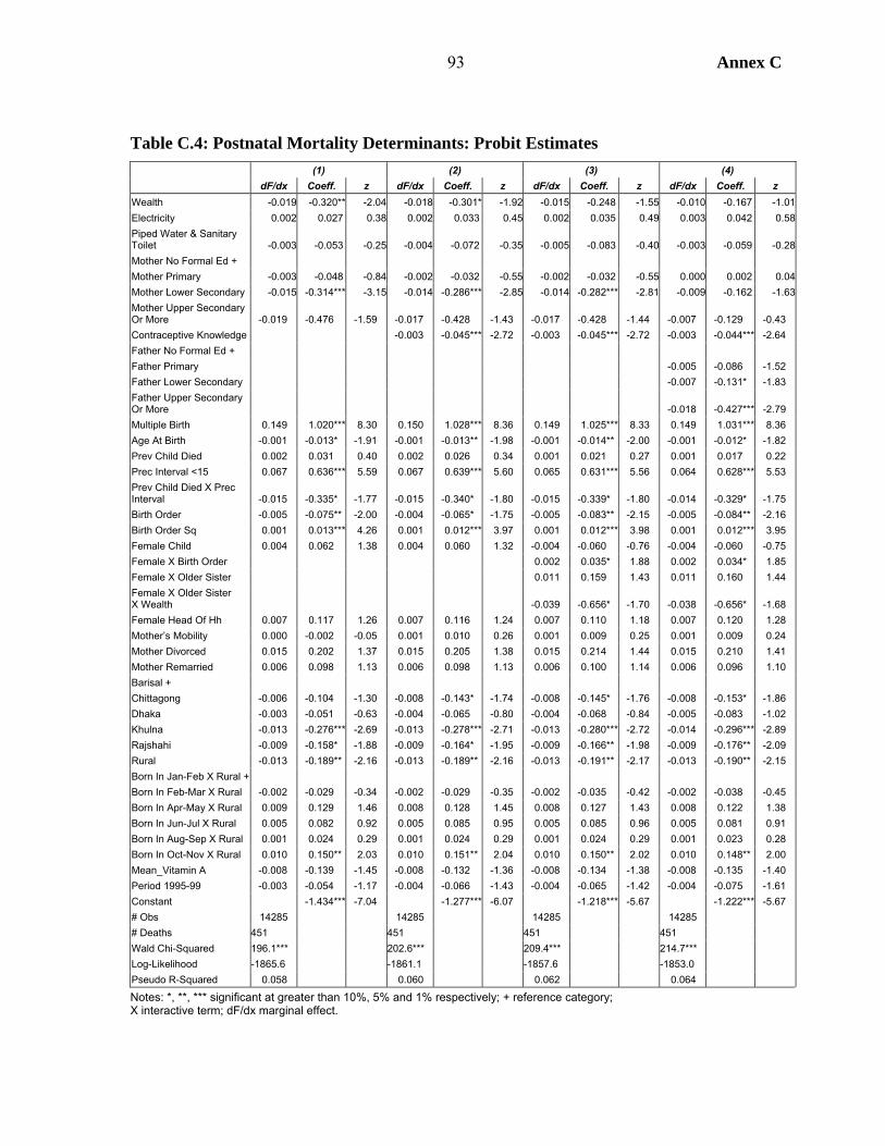
Annex C 93

Table C.4: Postnatal Mortality Determinants: Probit Estimates (1) (2) (3) (4) dF/dx Coeff. z dF/dx Coeff. z dF/dx Coeff. z dF/dx Coeff. z

Wealth -0.019 -0.320** -2.04 -0.018 -0.301* -1.92 -0.015 -0.248 -1.55 -0.010 -0.167 -1.01Electricity 0.002 0.027 0.38 0.002 0.033 0.45 0.002 0.035 0.49 0.003 0.042 0.58Piped Water & Sanitary Toilet -0.003 -0.053 -0.25 -0.004 -0.072 -0.35 -0.005 -0.083 -0.40 -0.003 -0.059 -0.28Mother No Formal Ed + Mother Primary -0.003 -0.048 -0.84 -0.002 -0.032 -0.55 -0.002 -0.032 -0.55 0.000 0.002 0.04Mother Lower Secondary -0.015 -0.314*** -3.15 -0.014 -0.286*** -2.85 -0.014 -0.282*** -2.81 -0.009 -0.162 -1.63Mother Upper Secondary Or More -0.019 -0.476 -1.59 -0.017 -0.428 -1.43 -0.017 -0.428 -1.44 -0.007 -0.129 -0.43 Contraceptive Knowledge -0.003 -0.045*** -2.72 -0.003 -0.045*** -2.72 -0.003 -0.044*** -2.64 Father No Formal Ed + Father Primary -0.005 -0.086 -1.52 Father Lower Secondary -0.007 -0.131* -1.83 Father Upper Secondary Or More -0.018 -0.427*** -2.79 Multiple Birth 0.149 1.020*** 8.30 0.150 1.028*** 8.36 0.149 1.025*** 8.33 0.149 1.031*** 8.36 Age At Birth -0.001 -0.013* -1.91 -0.001 -0.013** -1.98 -0.001 -0.014** -2.00 -0.001 -0.012* -1.82 Prev Child Died 0.002 0.031 0.40 0.002 0.026 0.34 0.001 0.021 0.27 0.001 0.017 0.22 Prec Interval <15 0.067 0.636*** 5.59 0.067 0.639*** 5.60 0.065 0.631*** 5.56 0.064 0.628*** 5.53 Prev Child Died X Prec Interval -0.015 -0.335* -1.77 -0.015 -0.340* -1.80 -0.015 -0.339* -1.80 -0.014 -0.329* -1.75 Birth Order -0.005 -0.075** -2.00 -0.004 -0.065* -1.75 -0.005 -0.083** -2.15 -0.005 -0.084** -2.16 Birth Order Sq 0.001 0.013*** 4.26 0.001 0.012*** 3.97 0.001 0.012*** 3.98 0.001 0.012*** 3.95 Female Child 0.004 0.062 1.38 0.004 0.060 1.32 -0.004 -0.060 -0.76 -0.004 -0.060 -0.75 Female X Birth Order 0.002 0.035* 1.88 0.002 0.034* 1.85 Female X Older Sister 0.011 0.159 1.43 0.011 0.160 1.44 Female X Older Sister X Wealth -0.039 -0.656* -1.70 -0.038 -0.656* -1.68 Female Head Of Hh 0.007 0.117 1.26 0.007 0.116 1.24 0.007 0.110 1.18 0.007 0.120 1.28 Mother’s Mobility 0.000 -0.002 -0.05 0.001 0.010 0.26 0.001 0.009 0.25 0.001 0.009 0.24 Mother Divorced 0.015 0.202 1.37 0.015 0.205 1.38 0.015 0.214 1.44 0.015 0.210 1.41 Mother Remarried 0.006 0.098 1.13 0.006 0.098 1.13 0.006 0.100 1.14 0.006 0.096 1.10 Barisal + Chittagong -0.006 -0.104 -1.30 -0.008 -0.143* -1.74 -0.008 -0.145* -1.76 -0.008 -0.153* -1.86 Dhaka -0.003 -0.051 -0.63 -0.004 -0.065 -0.80 -0.004 -0.068 -0.84 -0.005 -0.083 -1.02 Khulna -0.013 -0.276*** -2.69 -0.013 -0.278*** -2.71 -0.013 -0.280*** -2.72 -0.014 -0.296*** -2.89 Rajshahi -0.009 -0.158* -1.88 -0.009 -0.164* -1.95 -0.009 -0.166** -1.98 -0.009 -0.176** -2.09 Rural -0.013 -0.189** -2.16 -0.013 -0.189** -2.16 -0.013 -0.191** -2.17 -0.013 -0.190** -2.15 Born In Jan-Feb X Rural + Born In Feb-Mar X Rural -0.002 -0.029 -0.34 -0.002 -0.029 -0.35 -0.002 -0.035 -0.42 -0.002 -0.038 -0.45 Born In Apr-May X Rural 0.009 0.129 1.46 0.008 0.128 1.45 0.008 0.127 1.43 0.008 0.122 1.38 Born In Jun-Jul X Rural 0.005 0.082 0.92 0.005 0.085 0.95 0.005 0.085 0.96 0.005 0.081 0.91 Born In Aug-Sep X Rural 0.001 0.024 0.29 0.001 0.024 0.29 0.001 0.024 0.29 0.001 0.023 0.28 Born In Oct-Nov X Rural 0.010 0.150** 2.03 0.010 0.151** 2.04 0.010 0.150** 2.02 0.010 0.148** 2.00 Mean_Vitamin A -0.008 -0.139 -1.45 -0.008 -0.132 -1.36 -0.008 -0.134 -1.38 -0.008 -0.135 -1.40 Period 1995-99 -0.003 -0.054 -1.17 -0.004 -0.066 -1.43 -0.004 -0.065 -1.42 -0.004 -0.075 -1.61 Constant -1.434*** -7.04 -1.277*** -6.07 -1.218*** -5.67 -1.222*** -5.67 # Obs 14285 14285 14285 14285 # Deaths 451 451 451 451 Wald Chi-Squared 196.1*** 202.6*** 209.4*** 214.7*** Log-Likelihood -1865.6 -1861.1 -1857.6 -1853.0 Pseudo R-Squared 0.058 0.060 0.062 0.064

Notes: *, **, *** significant at greater than 10%, 5% and 1% respectively; + reference category; X interactive term; dF/dx marginal effect.

Annex C 94

47. There is some locational variation in postnatal mortality in multivariate analysis, as children in rural areas and in Khulna and Rajshahi have lower estimated mortality risk when controlling for other factors.23 The negative estimated impact of urban areas on postnatal survival may reflect that, accounting for socioeconomic factors and services, urban areas are more risky environment for infants, e.g., due to increased exposure to disease in areas of high population density, greater likelihood of poor communities being directly adversely affected by annual floods (e.g., because they are forced to live on river-banks), and due to greater environmental pollution. Seasonality is again a significant factor in rural areas: postnatal infants are more likely to die if born in the months of October and November, which is the counterpart to the higher neonatal mortality observed in December-January.

48. It is possible to account for (self-reported) annual food availability at household level and mother’s recollection of birth weight in the 1999/2000 survey round, as well as mother’s agency, using an index constructed from mother’s reported decisionmaking in the household.24 Table C.5 presents results for 1999/2000 survey data for infant mortality, which pools observations for neonates and postnates in order to maximize number of observed deaths. Specification (1) indicates that low birth weight (moderately small and very small) children are significantly more likely to die in the infant period, but whether the household experiences food deficit during some or all of the year has no significant effect on infant mortality. Specification (2) reports results for rural areas only and includes a variable indicating whether the household was situated in a Bangladesh Integrated Nutrition Project (BINP) area. While being in a BINP area does not significantly reduce infant mortality, the interaction with mother’s schooling suggests that better educated mothers are more able to benefit from the BINP project, e.g., because they are more likely to understand child growth charts and to follow educational messages such as beneficial food practices (see Annex G).25 In neither specification is mother’s agency significantly correlated with infant mortality.

23. Interactive terms between division of residence and gender are not significant determinants of postnatal mortality (results not reported).

24. The agency index is the simple sum of indicators of whether the woman has final say on own and children’s health care, household purchases for large items and daily needs, what should be cooked each day and visits to family, friends or relatives.

25. Another possibility is that wealthier households were better able to benefit from the BINP. However, an interactive term between BINP and wealth is insignificant, while the interaction between BINP and mother’s education remains significant. The same result is found for child mortality.

Annex C 95

Table C.5: Infant Mortality Determinants in 1999: Probit Estimates (1) (2 Rural) dF/dx Coeff. z dF/dx Coeff. z

Wealth -0.017 -0.156 -0.88 -0.009 -0.083 -0.40Electricity -0.007 -0.066 -0.78 -0.009 -0.083 -0.82Piped Water & Sanitary Toilet -0.017 -0.178 -0.66 Mother No Formal Ed + Mother Primary -0.016 -0.156** -2.14 -0.018 -0.171** -2.02Mother Lower Secondary -0.012 -0.111 -1.08 -0.001 -0.013 -0.12Mother Upper Secondary Or More -0.043 -0.621** -2.36 -0.044 -0.691 -1.59Contraceptive Knowledge -0.009 -0.081*** -3.97 -0.011 -0.097*** -4.14Multiple Birth 0.341 1.352*** 7.77 0.362 1.418*** 7.34Age At Birth -0.004 -0.038 -1.09 -0.002 -0.018 -0.45Age At Birth Sq 0.000 0.001 1.04 0.000 0.000 0.44Prev Child Died 0.000 0.002 0.02 -0.006 -0.054 -0.42Prec Interval <15 0.111 0.642*** 4.05 0.102 0.614*** 3.25Prev Child Died X Prec Interval -0.027 -0.302 -1.10 -0.014 -0.143 -0.47Birth Order -0.022 -0.200*** -3.45 -0.024 -0.218*** -3.27Birth Order Sq 0.002 0.017*** 3.26 0.002 0.018 3.10Female Child -0.009 -0.082 -1.46 -0.005 -0.049 -0.77Female Head Of Hh 0.006 0.055 0.44 0.001 0.008 0.06Mother’s Mobility -0.001 -0.005 -0.09 0.004 0.034 0.49Mother’s Agency 0.000 0.004 0.37 0.001 0.006 0.52Barisal + Chittagong -0.010 -0.091 -0.84 -0.011 -0.100 -0.83Dhaka -0.005 -0.046 -0.41 -0.009 -0.085 -0.68Khulna -0.024 -0.258** -2.05 -0.025 -0.269* -1.88Rajshahi -0.009 -0.080 -0.70 -0.008 -0.077 -0.61Rural -0.013 -0.113 -1.16 Born In Jan-Feb X Rural + Born In Feb-Mar X Rural -0.027 -0.287** -2.45 -0.027 -0.291** -2.47Born In Apr-May X Rural 0.001 0.006 0.06 0.000 0.003 0.03Born In Jun-Jul X Rural 0.000 -0.002 -0.01 0.001 0.006 0.05Born In Aug-Sep X Rural -0.003 -0.025 -0.25 -0.001 -0.009 -0.08Born In Oct-Nov X Rural -0.003 -0.027 -0.28 -0.002 -0.021 -0.23Mean_Vitamin A -0.018 -0.164 -1.49 -0.012 -0.106 -0.83Food Deficit 0.005 0.041 0.58 0.005 0.047 0.60Low Birth Weight 0.023 0.192*** 2.87 0.025 0.209*** 2.77Binp 0.022 0.180 1.01Binp X Mother’s Schooling -0.055 -0.509*** -2.87Constant -0.141 -0.300 -0.491 -0.94# obs 5626 4172 # deaths 382 289 Wald chi-squared 175.2*** 154.3*** Log-likelihood -1272.5 -939.7 Pseudo R-squared 0.080 0.087 Notes: *, **, *** significant at greater than 10%, 5% and 1% respectively; + reference category; X interactive term; dF/dx marginal effect.

Annex C 96

Child Mortality

49. Table C.6 presents multivariate analysis of child mortality using Cox proportional hazards model.26 The model is stratified by poverty status (where poverty is defined using a threshold of the wealth index), allowing the baseline hazard to differ between poor and non-poor.27 The most significant factors explaining differentials in child mortality are household wealth, vaccinations, and maternal education.

50. Coefficients on (non-self) community shares of children receiving Vitamin A supplementation and having no vaccinations have the expected signs, indicating that access to health services has a direct positive effect on child survival prospects. Formal education of mothers reduces child mortality risk, but in contrast with results for infants, the effect of mother’s knowledge of modern contraception is negative but insignificant in the child mortality regressions (specification 2); this may indicate contraceptive knowledge to be a better representation of knowledge of good care practices for infants regarding health care and feeding. Access to piped drinking water and sanitary toilet facilities negatively correlates with child mortality, though, somewhat surprisingly, this effect is insignificant. However, the interaction between schooling and water and sanitation is significantly negative, indicating complementarities in the improvement of child health status: intuitively, access to piped water and clean sanitation is unlikely to improve survival chances alone, mothers must know how to use facilities properly and children must also learn to use them, which is more likely where their mothers are educated. Maternal education becomes insignificant when controlling for paternal education (specification 4). Of the remaining mother-level variables, mobility is insignificant, but children of mothers who are remarried have significantly higher mortality risk, which may indicate children are at risk of being rejected by the new family.

51. The regressions indicate evidence for discrimination against girl children, who have significantly higher chances of dying than boys between age 1 and 5 years. Breaking down this effect, it is girls of higher birth order who fare worse (though, as estimated by the quadratic term, the birth order effect levels off after the sixth child) (specification 3). Children living in Khulna and Rajshahi Divisions have significantly better survival chances than elsewhere, while interactions with gender find that girls living in Chittagong Division face the highest levels of discrimination.

52. Maternal age at birth, birth order, and fate of previous child are all significantly correlated with child mortality risk; maternal age has a linear positive relationship and birth order a linear negative relationship with child mortality. These factors may reflect fertility and therefore be endogenous to mortality. Thus, specification (5) omits these variables, the main effect being to improve significance of education variables.

26. As well as the coefficients, hazard rates are reported, indicating the effect of a unit change in the explanatory variable on the risk of death in childhood.

27. A test for proportional hazards based on Schoenfeld residuals indicates the null hypothesis (that the proportional hazards assumption is not violated) is not rejected for each explanatory variable separately, while the joint test for all variables does not reject the null at p-value=0.62.

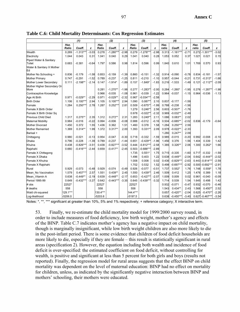
Annex C 97

Table C.6: Child Mortality Determinants: Cox Regression Estimates (1) (2) (3) (4) (5)

Haz. Ratio Coeff. z

Haz. Ratio Coeff. z

Haz. Ratio Coeff. z

Haz. ratio Coeff. z

Haz. ratio Coeff. z

Wealth 0.269 -1.313*** -3.03 0.278 -1.280*** -2.98 0.279 -1.278*** -2.98 0.313 -1.161*** -2.71 0.272 -1.301*** -3.02Electricity 1.044 0.043 0.31 1.041 0.040 0.29 1.041 0.040 0.28 1.053 0.052 0.37 1.021 0.021 0.15Piped Water & Sanitary Toilet 0.683 -0.381 -0.64 1.797 0.586 0.98 1.814 0.596 0.99 1.840 0.610 1.01 1.769 0.570 0.93Water & Sanitary X Mother Ed Mother No Schooling + 0.836 -0.179 -1.58 0.853 -0.159 -1.39 0.860 -0.151 -1.32 0.914 -0.090 -0.78 0.834 -0.181 -1.57Mother Primary 0.747 -0.291 -1.52 0.789 -0.237 -1.25 0.811 -0.210 -1.10 0.957 -0.044 -0.21 0.731 -0.313* -1.66Mother Lower Secondary 0.111 -2.198** -2.14 0.147 -1.914* -1.89 0.157 -1.849* -1.83 0.216 -1.533 -1.49 0.121 -2.112** -2.09Mother Higher Secondary Or More 0.281 -1.270** -1.98 0.277 -1.283** -2.00 0.284 -1.260* -1.95 0.276 -1.287** -1.98Contraceptive Knowledge 0.966 -0.035 -1.08 0.961 -0.039 -1.22 0.964 -0.037 -1.15 0.964 -0.036 -1.13Age At Birth 0.971 -0.029** -2.29 0.971 -0.029** -2.32 0.967 -0.034*** -2.58 Birth Order 1.106 0.100*** 2.94 1.105 0.100*** 2.94 1.090 0.087** 2.10 0.837 -0.177 -1.59 Female 1.284 0.250*** 2.78 1.287 0.252*** 2.81 0.509 -0.675** -1.99 0.788 -0.238 -1.56 Female X Birth Order 1.279 0.246** 2.56 0.603 -0.507* -1.76 Female X Birth Order Sq 0.978 -0.022** -2.32 0.969 -0.032** -2.49 Previous Child Died 1.317 0.275** 2.35 1.312 0.272** 2.31 1.283 0.249** 2.11 1.086 0.083** 2.02 Maternal Mobility 0.984 -0.016 -0.22 0.994 -0.006 -0.08 0.988 -0.012 -0.16 0.504 -0.685** -2.02 0.836 -0.179 -0.64Mother Divorced 1.450 0.372 1.55 1.436 0.362 1.51 1.460 0.378 1.58 1.284 0.250*** 2.59 Mother Remarried 1.369 0.314** 1.99 1.372 0.317** 2.00 1.393 0.331** 2.09 0.978 -0.022** -2.33 Barisal + 1.280 0.247** 2.09 Chittagong 0.980 -0.021 -0.13 0.954 -0.047 -0.30 0.718 -0.332 -1.59 0.985 -0.015 -0.20 0.992 -0.008 -0.10Dhaka 0.796 -0.228 -1.39 0.789 -0.237 -1.44 0.651 -0.429** -1.96 1.456 0.376 1.56 1.404 0.339 1.42Khulna 0.438 -0.826*** -3.51 0.438 -0.827*** -3.52 0.444 -0.812*** -2.58 1.385 0.326** 2.06 1.300 0.262* 1.66Rajshahi 0.660 -0.416*** -2.44 0.659 -0.417** -2.45 0.503 -0.688*** -2.89 Female X Chittagong 1.735 0.551* 1.75 0.715 -0.335 -1.60 0.717 -0.332 -1.59Female X Dhaka 1.496 0.403 1.22 0.638 -0.449** -2.04 0.642 -0.444** -2.02Female X Khulna 1.008 0.008 0.02 0.436 -0.829*** -2.63 0.443 -0.814*** -2.59Female X Rajshahi 1.702 0.532 1.52 0.498 -0.697*** -2.92 0.500 -0.692*** -2.91Rural 0.929 -0.073 -0.48 0.929 -0.074 -0.49 0.926 -0.077 -0.51 1.737 0.552* 1.76 1.748 0.559* 1.78Mean_No Vaccination 1.579 0.457*** 2.57 1.551 0.439** 2.45 1.550 0.439** 2.46 1.509 0.412 1.25 1.476 0.389 1.18Mean_Vitamin A 0.638 -0.449** -2.19 0.639 -0.448** -2.17 0.653 -0.427** -2.07 1.009 0.009 0.02 0.961 -0.040 -0.09Period 1995-99 0.649 -0.432*** -3.27 0.642 -0.443*** -3.35 0.645 -0.439*** -3.32 1.714 0.539 1.54 1.645 0.498 1.42# obs 22527 22527 22527 0.932 -0.071 -0.47 0.932 -0.070 -0.46# deaths 558 558 558 1.543 0.434** 2.43 1.568 0.450** 2.52Wald chi-squared 129.1*** 130.4*** 144.4*** 0.657 -0.420** -2.04 0.625 -0.470** -2.26Log-likelihood -5206.0 -5203.6 -5197.5 0.638 -0.450*** -3.40 0.627 -0.467*** -3.54

Notes: *, **, *** significant at greater than 10%, 5% and 1% respectively; + reference category; X interactive term. 53. Finally, we re-estimate the child mortality model for 1999/2000 survey round, in order to include measures of food deficiency, low birth weight, mother’s agency and effects of the BINP. Table C.7 indicates mother’s agency has a negative impact on child mortality, though is marginally insignificant, while low birth weight children are also more likely to die in the post-infant period. There is some evidence that children of food deficit households are more likely to die, especially if they are female – this result is statistically significant in rural areas (specification 2). However, the equation including both wealth and incidence of food deficit is over-specified: the estimated coefficient on food deficit, without controlling for wealth, is positive and significant at less than 5 percent for both girls and boys (results not reported). Finally, the regression model for rural areas suggests that the effect BINP on child mortality was dependent on the level of maternal education: BINP had no effect on mortality for children, unless, as indicated by the significantly negative interaction between BINP and mothers’ schooling, their mothers were educated.

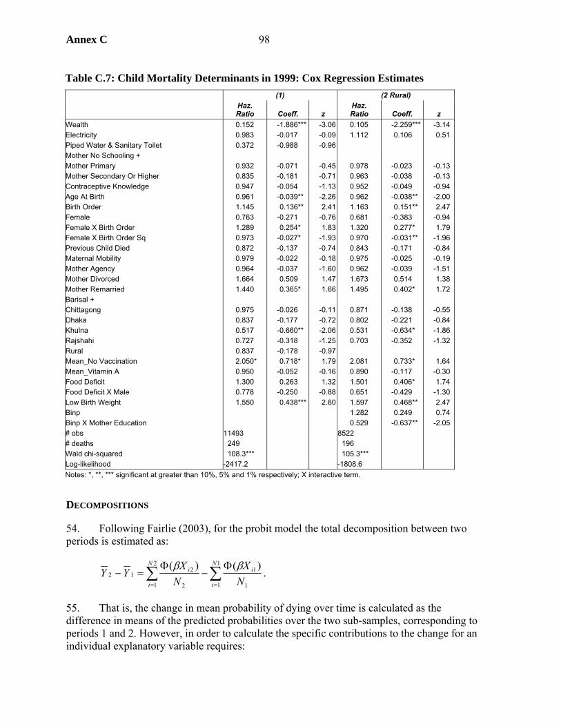
Annex C 98

Table C.7: Child Mortality Determinants in 1999: Cox Regression Estimates (1) (2 Rural)

Haz. Ratio Coeff. z

Haz. Ratio Coeff. z

Wealth 0.152 -1.886*** -3.06 0.105 -2.259*** -3.14 Electricity 0.983 -0.017 -0.09 1.112 0.106 0.51 Piped Water & Sanitary Toilet 0.372 -0.988 -0.96 Mother No Schooling + Mother Primary 0.932 -0.071 -0.45 0.978 -0.023 -0.13 Mother Secondary Or Higher 0.835 -0.181 -0.71 0.963 -0.038 -0.13 Contraceptive Knowledge 0.947 -0.054 -1.13 0.952 -0.049 -0.94 Age At Birth 0.961 -0.039** -2.26 0.962 -0.038** -2.00 Birth Order 1.145 0.136** 2.41 1.163 0.151** 2.47 Female 0.763 -0.271 -0.76 0.681 -0.383 -0.94 Female X Birth Order 1.289 0.254* 1.83 1.320 0.277* 1.79 Female X Birth Order Sq 0.973 -0.027* -1.93 0.970 -0.031** -1.96 Previous Child Died 0.872 -0.137 -0.74 0.843 -0.171 -0.84 Maternal Mobility 0.979 -0.022 -0.18 0.975 -0.025 -0.19 Mother Agency 0.964 -0.037 -1.60 0.962 -0.039 -1.51 Mother Divorced 1.664 0.509 1.47 1.673 0.514 1.38 Mother Remarried 1.440 0.365* 1.66 1.495 0.402* 1.72 Barisal + Chittagong 0.975 -0.026 -0.11 0.871 -0.138 -0.55 Dhaka 0.837 -0.177 -0.72 0.802 -0.221 -0.84 Khulna 0.517 -0.660** -2.06 0.531 -0.634* -1.86 Rajshahi 0.727 -0.318 -1.25 0.703 -0.352 -1.32 Rural 0.837 -0.178 -0.97 Mean_No Vaccination 2.050* 0.718* 1.79 2.081 0.733* 1.64 Mean_Vitamin A 0.950 -0.052 -0.16 0.890 -0.117 -0.30 Food Deficit 1.300 0.263 1.32 1.501 0.406* 1.74 Food Deficit X Male 0.778 -0.250 -0.88 0.651 -0.429 -1.30 Low Birth Weight 1.550 0.438*** 2.60 1.597 0.468** 2.47 Binp 1.282 0.249 0.74 Binp X Mother Education 0.529 -0.637** -2.05 # obs 11493 8522 # deaths 249 196 Wald chi-squared 108.3*** 105.3*** Log-likelihood -2417.2 -1808.6 Notes: *, **, *** significant at greater than 10%, 5% and 1% respectively; X interactive term.

DECOMPOSITIONS

54. Following Fairlie (2003), for the probit model the total decomposition between two periods is estimated as:

∑∑==

Φ−

Φ=−

1

1 1

12

1 2

212

)()( N

i

iN

i

i

NX

NX

YYββ

.

55. That is, the change in mean probability of dying over time is calculated as the difference in means of the predicted probabilities over the two sub-samples, corresponding to periods 1 and 2. However, in order to calculate the specific contributions to the change for an individual explanatory variable requires:

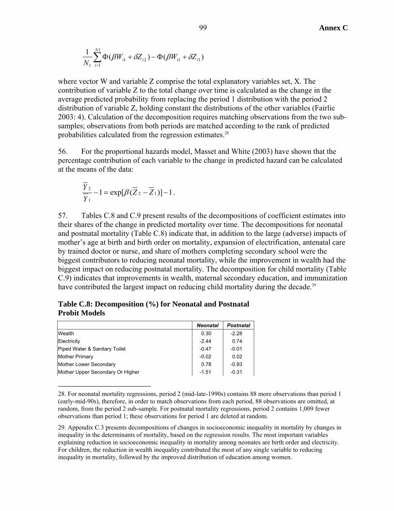
Annex C 99

)()(111

1

121

1ii

N

iii ZWZW

Nδβδβ +Φ−+Φ∑

=

where vector W and variable Z comprise the total explanatory variables set, X. The contribution of variable Z to the total change over time is calculated as the change in the average predicted probability from replacing the period 1 distribution with the period 2 distribution of variable Z, holding constant the distributions of the other variables (Fairlie 2003: 4). Calculation of the decomposition requires matching observations from the two sub-samples; observations from both periods are matched according to the rank of predicted probabilities calculated from the regression estimates.28

56. For the proportional hazards model, Masset and White (2003) have shown that the percentage contribution of each variable to the change in predicted hazard can be calculated at the means of the data:

1)](exp[1 121

2 −−=− ZZYY β .

57. Tables C.8 and C.9 present results of the decompositions of coefficient estimates into their shares of the change in predicted mortality over time. The decompositions for neonatal and postnatal mortality (Table C.8) indicate that, in addition to the large (adverse) impacts of mother’s age at birth and birth order on mortality, expansion of electrification, antenatal care by trained doctor or nurse, and share of mothers completing secondary school were the biggest contributors to reducing neonatal mortality, while the improvement in wealth had the biggest impact on reducing postnatal mortality. The decomposition for child mortality (Table C.9) indicates that improvements in wealth, maternal secondary education, and immunization have contributed the largest impact on reducing child mortality during the decade.29

Table C.8: Decomposition (%) for Neonatal and Postnatal Probit Models Neonatal Postnatal Wealth 0.30 -2.28 Electricity -2.44 0.74 Piped Water & Sanitary Toilet -0.47 -0.01 Mother Primary -0.02 0.02 Mother Lower Secondary 0.78 -0.93 Mother Upper Secondary Or Higher -1.51 -0.31

28. For neonatal mortality regressions, period 2 (mid-late-1990s) contains 88 more observations than period 1 (early-mid-90s), therefore, in order to match observations from each period, 88 observations are omitted, at random, from the period 2 sub-sample. For postnatal mortality regressions, period 2 contains 1,009 fewer observations than period 1; these observations for period 1 are deleted at random.

29. Appendix C.3 presents decompositions of changes in socioeconomic inequality in mortality by changes in inequality in the determinants of mortality, based on the regression results. The most important variables explaining reduction in socioeconomic inequality in mortality among neonates are birth order and electricity. For children, the reduction in wealth inequality contributed the most of any single variable to reducing inequality in mortality, followed by the improved distribution of education among women.

Annex C 100

Table C.8: Decomposition (%) for Neonatal and Postnatal Probit Models Neonatal Postnatal Contraceptive Knowledge 0.12 3.01 Multiple Birth 0.85 4.13 Age At Birth 14.62 3.79 Age At Birth Sq 14.89 Prev Child Died -0.88 -0.14 Prec Interval <15 0.76 4.50 Prev Child Died X Prec Interval 2.00 2.01 Birth Order 39.12 21.88 Birth Order Sq 2.17 13.52 Female Child 0.49 0.63 Female X Birth Order 0.18 Female X Older Sister 0.94 Female X Older Sister X Wealth 0.28 Female Head Of Hh 0.00 0.08 Mother’s Mobility -0.78 0.20 Mother Divorced 0.03 -0.38 Mother Remarried 0.07 -0.05 Antenatal Visits By Doctor/Nurse -4.27 Chittagong -0.26 -0.40 Dhaka 0.27 1.34 Khulna -0.35 -0.76 Rajshahi 0.28 2.19 Rural 0.79 5.72 Born In Feb-Mar X Rural 0.56 0.20 Born In Apr-May X Rural 0.83 0.03 Born In Jun-Jul X Rural 0.17 0.01 Born In Aug-Sep X Rural 0.45 -0.04 Born In Oct-Nov X Rural 0.18 0.61 Mean_Vitamin A -0.65

COST EFFECTIVENESS ANALYSIS

58. Analysis of cost effectiveness requires an estimate of the actual number of lives saved by an intervention. Table C.10 shows the actual numbers which are used as the base case for the simulations. Data on population, crude birth rate, and infant and child mortality are taken from Khan and Yoder (1998) and the World Development Indicators database. The crude birth rate is used to calculate the number of live births each year. The infant mortality rate can be used to calculate how many of those born in each year will die as infants, giving total infant deaths. Where necessary for the calculations it is assumed that half of infant deaths are neonatal (figures not shown). It is thus possible to calculate how many of the children born that year survive to age one. Using the CMR it can be calculated how many of those children will die before their fifth birthday. These deaths are spread over the four years in the proportions, 0.5, 0.3, 0.15, and 0.05. Hence, the number of child deaths each year can be calculated. These can be added to infant deaths to get under-five deaths (not shown).

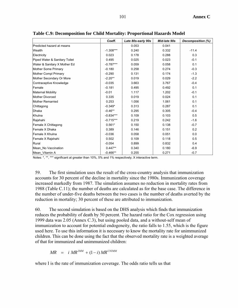
Annex C 101

Table C.9: Decomposition for Child Mortality: Proportional Hazards Model Coeff. Late 80s-early 90s Mid-late 90s Decomposition (%)

Predicted hazard at means 0.053 0.041 Wealth -1.308*** 0.240 0.332 -11.4 Electricity 0.023 0.178 0.288 0.3 Piped Water & Sanitary Toilet 0.495 0.025 0.023 -0.1 Water & Sanitary X Mother Ed -0.787*** 0.059 0.058 0.1 Mother Some Primary -0.180 0.258 0.274 -0.3 Mother Compl Primary -0.290 0.131 0.174 -1.3 Mother Secondary Or More -2.20** 0.019 0.029 -2.2 Contraceptive Knowledge -0.035 3.663 3.767 -0.4 Female -0.181 0.495 0.492 0.1 Maternal Mobility -0.01 1.117 1.202 -0.1 Mother Divorced 0.335 0.019 0.024 0.1 Mother Remarried 0.253 1.056 1.061 0.1 Chittagong -0.349* 0.313 0.287 0.1 Dhaka -0.46** 0.295 0.305 -0.4 Khulna -0.834*** 0.109 0.103 0.5 Rajshahi -0.715*** 0.219 0.242 -1.6 Female X Chittagong 0.561* 0.150 0.138 -0.7 Female X Dhaka 0.389 0.146 0.151 0.2 Female X Khulna -0.036 0.058 0.051 0.0 Female X Rajshahi 0.502 0.109 0.118 0.5 Rural -0.054 0.899 0.832 0.4 Mean_No Vaccination 0.447** 0.340 0.180 -6.9 Mean_Vitamin A -0.466** 0.255 0.271 -0.7 Notes: *, **, *** significant at greater than 10%, 5% and 1% respectively; X interactive term.

59. The first simulation uses the result of the cross-country analysis that immunization accounts for 30 percent of the decline in mortality since the 1980s. Immunization coverage increased markedly from 1987. The simulation assumes no reduction in mortality rates from 1988 (Table C.11); the number of deaths are calculated as for the base case. The difference in the number of under-five deaths between the two cases is the number of deaths averted by the reduction in mortality; 30 percent of these are attributed to immunization.

60. The second simulation is based on the DHS analysis which finds that immunization reduces the probability of death by 50 percent. The hazard ratio for the Cox regression using 1999 data was 2.05 (Annex C.3), but using pooled data, and a without-self mean of immunization to account for potential endogeneity, the ratio falls to 1.55, which is the figure used here. To use this information it is necessary to know the mortality rate for unimmunized children. This can be done using the fact that the observed mortality rate is a weighted average of that for immunized and unimmunized children:

UNIMMIMM MRiMRiMR )1( −+=

where I is the rate of immunization coverage. The odds ratio tells us that

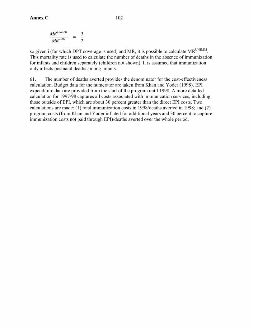
Annex C 102

23

=IMM

UNIMM

MRMR

so given i (for which DPT coverage is used) and MR, it is possible to calculate MRUNIMM. This mortality rate is used to calculate the number of deaths in the absence of immunization for infants and children separately (children not shown). It is assumed that immunization only affects postnatal deaths among infants.

61. The number of deaths averted provides the denominator for the cost-effectiveness calculation. Budget data for the numerator are taken from Khan and Yoder (1998). EPI expenditure data are provided from the start of the program until 1998. A more detailed calculation for 1997/98 captures all costs associated with immunization services, including those outside of EPI, which are about 30 percent greater than the direct EPI costs. Two calculations are made: (1) total immunization costs in 1998/deaths averted in 1998; and (2) program costs (from Khan and Yoder inflated for additional years and 30 percent to capture immunization costs not paid through EPI)/deaths averted over the whole period.

103 Annex C

Table C.10: Under-Five Death Calculation Based on Actual Data (base case)

Year Population IMR CMR

Crude birth rate

No. of children

born Infant deaths

Children alive at age one

Child deaths of this cohort

Year 1 (.5)

Year 2 (.3)

Year 3 (.15)

Year 4 (.05)

Child deaths

per year 1981 89912 126 83.9 43.0 3866 485 3381 284 142 85 43 14 1982 92061 122 80.6 42.0 3867 472 3395 274 137 82 41 14 1983 94169 119 77.2 41.0 3861 458 3403 263 131 79 39 13 1984 96335 115 73.8 40.0 3853 444 3409 252 126 75 38 13 260 1985 98531 112 70.4 39.0 3843 430 3412 240 120 72 36 12 249 1986 100758 113 63.0 38.0 3829 431 3398 214 107 64 32 11 230 1987 103025 113 55.6 37.0 3812 431 3381 188 94 56 28 9 207 1988 105282 107 54.8 35.6 3744 402 3342 183 91 55 27 9 192 1989 107587 102 53.9 34.1 3671 373 3298 178 89 53 27 9 183 1990 109922 96 53.1 32.7 3592 345 3247 172 86 52 26 9 176 1991 111455 92 47.0 31.2 3482 320 3162 149 74 45 22 7 162 1992 113729 88 40.9 29.8 3389 298 3091 127 63 38 19 6 143 1993 115981 84 41.7 29.5 3417 287 3130 131 65 39 20 7 134 1994 118161 80 43.0 29.1 3441 274 3167 136 68 41 20 7 134 1995 120382 75 44.3 28.8 3465 260 3205 142 71 43 21 7 138 1996 122561 71 41.3 28.4 3486 247 3239 134 67 40 20 7 137 1997 124706 67 38.4 28.1 3504 233 3271 125 63 38 19 6 131 1998 126579 62 35.4 28.1 3559 222 3337 118 59 35 18 6 124 1999 128797 58 32.5 28.1 3624 211 3413 111 55 33 17 6 116 2000 131050 54 29.6 28.2 3690 199 3491 103 52 31 15 5 109 2001 133345 51 27.9 28.2 3758 192 3566 100 50 30 15 5 103 2002 135684 48 26.3 28.2 3826 184 3643 96 48 29 14 5 99

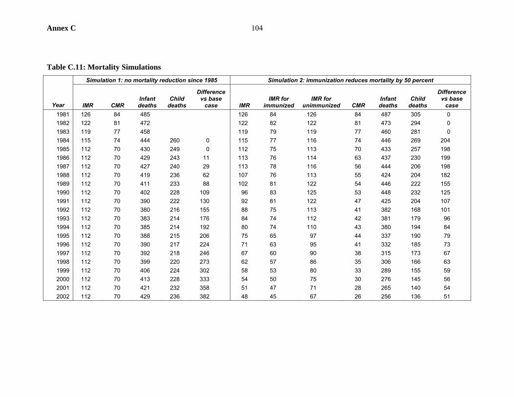
Annex C 104

Table C.11: Mortality Simulations Simulation 1: no mortality reduction since 1985 Simulation 2: immunization reduces mortality by 50 percent

Year IMR CMR Infant deaths

Child deaths

Difference vs base

case IMR IMR for

immunized IMR for

unimmunized CMR Infant deaths

Child deaths

Difference vs base

case 1981 126 84 485 126 84 126 84 487 305 0 1982 122 81 472 122 82 122 81 473 294 0 1983 119 77 458 119 79 119 77 460 281 0 1984 115 74 444 260 0 115 77 116 74 446 269 204 1985 112 70 430 249 0 112 75 113 70 433 257 198 1986 112 70 429 243 11 113 76 114 63 437 230 199 1987 112 70 427 240 29 113 78 116 56 444 206 198 1988 112 70 419 236 62 107 76 113 55 424 204 182 1989 112 70 411 233 88 102 81 122 54 446 222 155 1990 112 70 402 228 109 96 83 125 53 448 232 125 1991 112 70 390 222 130 92 81 122 47 425 204 107 1992 112 70 380 216 155 88 75 113 41 382 168 101 1993 112 70 383 214 176 84 74 112 42 381 179 96 1994 112 70 385 214 192 80 74 110 43 380 194 84 1995 112 70 388 215 206 75 65 97 44 337 190 79 1996 112 70 390 217 224 71 63 95 41 332 185 73 1997 112 70 392 218 246 67 60 90 38 315 173 67 1998 112 70 399 220 273 62 57 86 35 306 166 63 1999 112 70 406 224 302 58 53 80 33 289 155 59 2000 112 70 413 228 333 54 50 75 30 276 145 56 2001 112 70 421 232 358 51 47 71 28 265 140 54 2002 112 70 429 236 382 48 45 67 26 256 136 51

Annex C105

62. The results of these calculations are summarized in Table C.12. The range is quite large, from just under US$100 to nearly US$300 per life saved. These results compare with the US$137 reported by Khan and Yoder (1998). These calculations suggest that that result may be something of an underestimate, but that a value of US$200 per life saved is not unreasonable.

CONCLUSIONS

63. The exercise to examine the determinants of mortality in the neonatal, postnatal, and child periods has yielded some interesting results:

• Household incomes, as represented in this paper by wealth, exert a significant effect on post-neonatal survival, particularly in post-infancy when income contributed the most of any one variable to reducing mortality over time.

• Mothers’ education is an important factor behind variation in mortality risk across children and over time. Mothers’ education, particularly at secondary or higher level, has a significantly positive impact on child survival; this is observed over the impact of household wealth, as well as mothers’ knowledge of modern contraception, an indicator of general health knowledge, which itself is a significant determinant of infant mortality differentials. The results suggest that mother’s health knowledge has an important effect on survival chances, but also that children of better educated mothers are more likely to survive. The latter may be due to more highly educated mothers having greater say in household decisionmaking. Evidence also indicates that neonates have better survival chances when their mother is free to leave the dwelling and visit the health center, while divorce and remarriage can be detrimental to survival in childhood.

• Health services contribute significantly to improving childhood survival chances. Mortality is lower among newborns whose mothers attended antenatal visits with a trained doctor or nurse and immunization had a strong impact on reducing mortality in childhood in Bangladesh in the 1990s. These effects are robust to use of methods that attempt to account for endogeneity and unobserved heterogeneity in mothers’ preferences.

• Access to piped drinking water and sanitary toilet facilities were found to have a significant effect on reducing mortality among neonates, and among children in households where the mother has formal schooling.

• The multivariate analysis indicates that gender discrimination against girls remains strong. While the effect is quantitatively greatest among children, as would be expected, the evidence suggests that higher birth order girls are more likely to die in both the postnatal and post-infant periods. Analysis of DHS 1999/2000 data indicated that girl children in food deficit households are more likely to be discriminated against.

• The analysis of DHS 1999/2000 survey round data showed that infants and children living in BINP areas tended to have better survival chances where their mothers were formally educated, suggesting educated mothers were more able to understand and act upon the messages of the project and/or were more likely to take complementary actions such as use modern medical care.

Table C.12: Simulations of Costs of Saving One Life

Simulation 1 Simulation 2 1998 only 224 292 Whole program 192 90

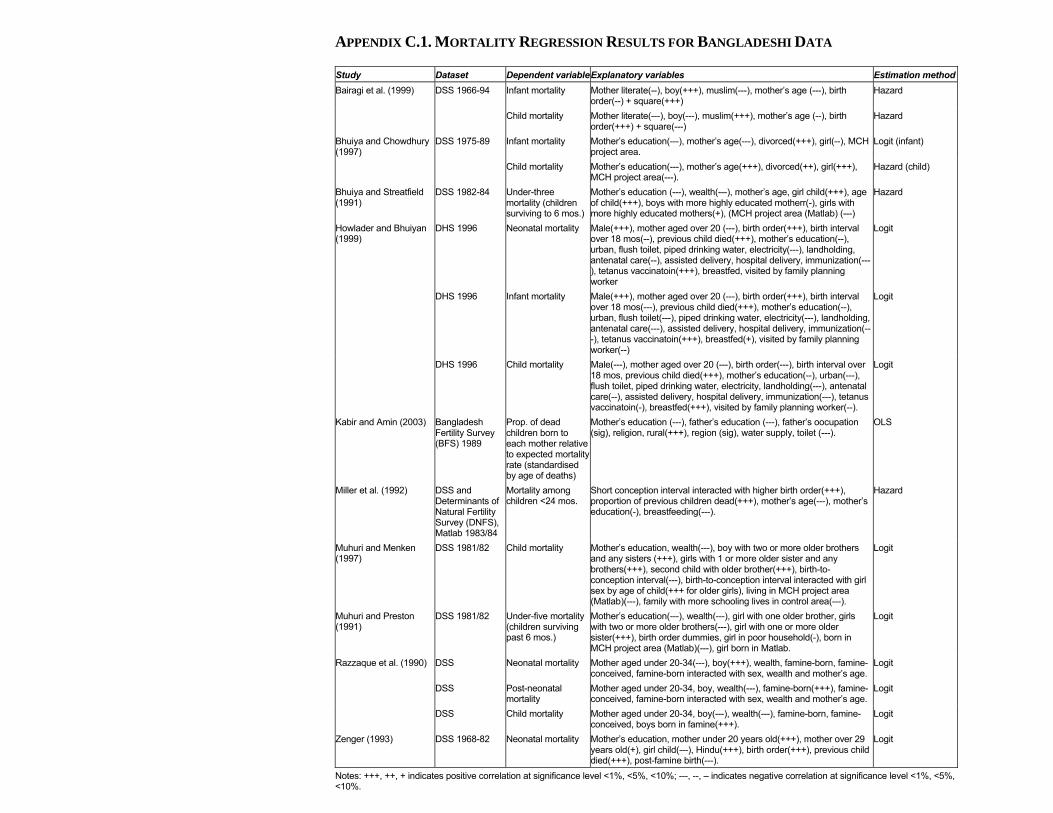
APPENDIX C.1. MORTALITY REGRESSION RESULTS FOR BANGLADESHI DATA

Study Dataset Dependent variableExplanatory variables Estimation methodBairagi et al. (1999) DSS 1966-94 Infant mortality Mother literate(--), boy(+++), muslim(---), mother’s age (---), birth

order(--) + square(+++) Hazard

Child mortality Mother literate(---), boy(---), muslim(+++), mother’s age (--), birth order(+++) + square(---)

Hazard

Bhuiya and Chowdhury (1997)

DSS 1975-89 Infant mortality Mother’s education(---), mother’s age(---), divorced(+++), girl(--), MCH project area.

Logit (infant)

Child mortality Mother’s education(---), mother’s age(+++), divorced(++), girl(+++), MCH project area(---).

Hazard (child)

Bhuiya and Streatfield (1991)

DSS 1982-84 Under-three mortality (children surviving to 6 mos.)

Mother’s education (---), wealth(---), mother’s age, girl child(+++), age of child(+++), boys with more highly educated motherr(-), girls with more highly educated mothers(+), (MCH project area (Matlab) (---)

Hazard

Howlader and Bhuiyan (1999)

DHS 1996 Neonatal mortality Male(+++), mother aged over 20 (---), birth order(+++), birth interval over 18 mos(--), previous child died(+++), mother’s education(--), urban, flush toilet, piped drinking water, electricity(---), landholding, antenatal care(--), assisted delivery, hospital delivery, immunization(---), tetanus vaccinatoin(+++), breastfed, visited by family planning worker

Logit

DHS 1996 Infant mortality Male(+++), mother aged over 20 (---), birth order(+++), birth interval over 18 mos(---), previous child died(+++), mother’s education(--), urban, flush toilet(---), piped drinking water, electricity(---), landholding, antenatal care(---), assisted delivery, hospital delivery, immunization(---), tetanus vaccinatoin(+++), breastfed(+), visited by family planning worker(--)

Logit

DHS 1996 Child mortality Male(---), mother aged over 20 (---), birth order(---), birth interval over 18 mos, previous child died(+++), mother’s education(--), urban(---), flush toilet, piped drinking water, electricity, landholding(---), antenatal care(--), assisted delivery, hospital delivery, immunization(---), tetanus vaccinatoin(-), breastfed(+++), visited by family planning worker(--).

Logit

Kabir and Amin (2003) Bangladesh Fertility Survey (BFS) 1989

Prop. of dead children born to each mother relative to expected mortality rate (standardised by age of deaths)

Mother’s education (---), father’s education (---), father’s oocupation (sig), religion, rural(+++), region (sig), water supply, toilet (---).

OLS

Miller et al. (1992) DSS and Determinants of Natural Fertility Survey (DNFS), Matlab 1983/84

Mortality among children <24 mos.

Short conception interval interacted with higher birth order(+++), proportion of previous children dead(+++), mother’s age(---), mother’s education(-), breastfeeding(---).

Hazard

Muhuri and Menken (1997)

DSS 1981/82 Child mortality Mother’s education, wealth(---), boy with two or more older brothers and any sisters (+++), girls with 1 or more older sister and any brothers(+++), second child with older brother(+++), birth-to-conception interval(---), birth-to-conception interval interacted with girl sex by age of child(+++ for older girls), living in MCH project area (Matlab)(---), family with more schooling lives in control area(---).

Logit

Muhuri and Preston (1991)

DSS 1981/82 Under-five mortality (children surviving past 6 mos.)

Mother’s education(---), wealth(---), girl with one older brother, girls with two or more older brothers(---), girl with one or more older sister(+++), birth order dummies, girl in poor household(-), born in MCH project area (Matlab)(---), girl born in Matlab.

Logit

Razzaque et al. (1990) DSS Neonatal mortality Mother aged under 20-34(---), boy(+++), wealth, famine-born, famine-conceived, famine-born interacted with sex, wealth and mother’s age.

Logit

DSS Post-neonatal mortality

Mother aged under 20-34, boy, wealth(---), famine-born(+++), famine-conceived, famine-born interacted with sex, wealth and mother’s age.

Logit

DSS Child mortality Mother aged under 20-34, boy(---), wealth(---), famine-born, famine-conceived, boys born in famine(+++).

Logit

Zenger (1993) DSS 1968-82 Neonatal mortality Mother’s education, mother under 20 years old(+++), mother over 29 years old(+), girl child(---), Hindu(+++), birth order(+++), previous child died(+++), post-famine birth(---).

Logit

Notes: +++, ++, + indicates positive correlation at significance level <1%, <5%, <10%; ---, --, – indicates negative correlation at significance level <1%, <5%, <10%.

Annex C

107

APPENDIX C.2. MEASURING SOCIOECONOMIC STATUS: WEALTH, ASSETS, AND WELFARE OUTCOMES IN BANGLADESH

64. This paper reviews measures of socioeconomic status (SES), with a particular focus on wealth. The objective is to provide guidance in constructing a suitable index, which can be used to measure SES using Demographic and Health Surveys (DHS). DHS collect data on asset ownership at the household level, which can be converted into indicators of household wealth status. There are various ways of doing this, and indices have been constructed from different types of assets using different estimation methodologies. However, attention to methodology is important because alternative indices have been shown not only to identify different households as “poor,” but also to generate significantly different measures of health inequality between “non-poor” and “poor.” This paper reviews the types of indicators that are usually used for socioeconomic status, focusing specifically on assets to measure SES and summarizes the issues involved in aggregating assets into a composite index of wealth. Finally, the paper presents results of construction of an asset index for Bangladesh DHS data.

Indicators of Socioeconomic Status

65. Socioeconomic status is a well-established term, originating in sociological literature (see Bollen et al. 1999).1 Socioeconomic status (SES) can be broadly defined as indicating an individual or household’s relative position according to some social and/or economic stratification scale, where the latter may be determined with reference to a broad or narrow set of characteristics. The term “status” implies a relative approach to measuring well-being, though some measures, such as income/consumption, can be interpreted absolutely, given adjustments for differences across space and time. Given this conceptual ambiguity, socioeconomic status is measured in a variety of ways, the most common being with economic indicators (such as income, expenditure, and asset ownership). This is because economic indicators are relatively easy to measure – unlike concepts of social standing, which are measured with much greater difficulty if at all – and because social and economic indicators are assumed to be strongly correlated. However, most studies also account for factors that arguably reflect social standing to a greater extent than income/wealth alone, including human capital and/or occupation.

66. Household income and consumption expenditure are the most commonly used measures of living standards. Consumption and income are estimated from surveys, such as the World Bank-sponsored Living Standards Measurement Surveys (LSMS), which collect detailed household-level information on income and consumption items, including imputed estimates of self-employed income and consumption of own produce. White and Masset (2003) provide a description of the steps that must be taken to ensure comparability of income and expenditure across households and time.

1. Bollen et al. (1999: 4) state that the term socioeconomic status “appears to have become commonplace only after the U.S. Census Bureau published a report in 1964 using a composite SES index for comparison of different groups.”

Annex C 108

67. Indicators of physical asset ownership such as durable goods, housing quality, and access to basic services such as water and sanitation, are often used to measure socioeconomic status where income or expenditure data are unavailable, as in the case of research based on Demographic and Health Survey (DHS) data. DHS collect nationally representative information on health, nutrition, and fertility. The DHS asset module can be used to construct an index of wealth, though the main problem is in aggregation, since data on prices, which would facilitate comparisons of different assets, are not available. There are also issues regarding the choice of assets to include in the index and adjustment for household size, composition, and economies of scale. These topics are take up below.

68. However, it should be clear that income/consumption and assets are not equivalent indicators. There is a theoretical justification for using assets to measure SES. Economic theory distinguishes current income from permanent income (wealth), the latter providing a better representation of living standards over time. If credit and insurance markets operated perfectly (and foresight were perfect), households would be able to plan expenditures and borrow/save accordingly to minimize consumption fluctuations across seasons and over economic and life cycles, in order to stabilize life-time consumption. Under these conditions, current expenditure provides the best indication of permanent income (wealth). In practice, though, particularly in poor countries, household expenditure tends to fluctuate with current income because problems in saving and borrowing (and accessing insurance) prevent consumption smoothing over time (Baulch and Hoddinott 2000).2 Under such conditions, assets are preferable to consumption for measuring wealth, and there is some empirical evidence supporting this; for example using survey data from Indonesia, Nepal and Pakistan, Filmer and Pritchett (1998) argue assets to be preferable to consumption for measuring wealth because they rank households more consistently over time.

69. On the other hand, income represents human capital attainment and remittance flows – important determinants of current living standards that physical assets are less likely to account for. Note also that, for these reasons, the stock of physical wealth would tend to be more unequally distributed than income flows. Human capital assets have been included in asset indices by some (Sahn and Stifel 2000) to reduce the bias in measuring wealth when relying on physical assets alone; the problem with doing so is that it precludes estimation of a separate education effect.

2. There is also the problem of lumpy consumption items – expenditure data collected in household surveys will be sensitive to large non-recurring consumption items such as healthcare bills, which would tend to artificially inflate the household’s estimated welfare, particularly if during the preceding or subsequent period the household saved for the item by reducing expenditure. While measures are usually taken when constructing household expenditure aggregates to exclude some non-recurring items, it has often been argued that because of these problems household expenditure data are satisfactory for calculating poverty levels, as these differences get ironed out, but not good at identifying poor households (Grosh and Glewwe 2000). Under these circumstances, wealth may be a better indicator of differences in current income across households, and assets are a better predictor of this. The problem with wealth is that the data collected on assets are usually limited (e.g., do not include financial savings), and in poorer countries, all the better-off have most or all of the items and many of the poorest have none, making it difficult to distinguish between them.

Annex C

109

Generating an Index

70. This section describes the main issues in generating an index from asset data collected by household surveys.

71. Before moving on it is important to note that there is no reason to generate an index unless it is needed for some analytical purpose, e.g., in order to analyze the relationship between “wealth” and another variable. If not, and household wealth merely needs to be controlled for, assets can enter separately in regressions. The main arguments against this are: (1) reduction in degrees of freedom, but this is not usually an issue with analysis of household survey data sets, given that the number of observations is often in the thousands; and (2) a high correlation between the different assets will result in multicollinearity, undermining their statistical significance.

72. Where households need to be ranked by wealth, in order to determine the correlation between wealth and another variable, an index can be generated by aggregating assets:

Ai = ψ1 ai1 + … + ψn ai n (1)

where Ai is the total asset score for each household i, an are individual asset types and ψn are the weights. Variables indicating ownership/access to assets are measured categorically (1 = yes; 0 = no). In all other cases, scale equivalence must be ensured, where necessary by adjusting variables to range between 0 and 1, otherwise the index will contain “hidden weights” since variables ranging over bigger scales will implicitly be weighted more heavily.3 Young Lives (2002) cites as an example of the latter the education component of UNDP’s Human Development Index (which is measured as one-third mean years of schooling to two-thirds literacy), which in the first year of implementation failed to adjust for scale equivalence of literacy (measured in percentage terms) and mean years of schooling (ranging between about 2 and 10); in the resulting education index, the majority of variation was due to literacy because of its much greater variance. One problem with rescaling is that it is sensitive to outliers, which may therefore have to be removed from the data beforehand.

73. The following hypothetical example (Table C2.1) demonstrates the calculation of a wealth score for two households, assuming a simple index of seven household durable goods (ownership of a wardrobe, chair, and table, which all have unitary weights, ownership of telephone, TV, and bicycle, which each carry weights of 2 and ownership of a motor vehicle, with weight 3). Household 1 owning all of the items would therefore have asset score 12; household 2 owning chair, table, and bicycle would be given an asset score of 4.

3. Young Lives (2002) gives a formula for scaling a variable X between 0 and 1, where welfare increases with X:

Xi* = (Xi – Xmin)/(Xmax – Xmin)

where Xi* denotes the scaled observation of individual i in variable X, and min and max refer to the respective minimum and maximum of variable X. To ensure spatial and temporal comparability, the minima and maxima may have to be pre-set rather than determined by the data.

Annex C 110

74. In the preceding example, weightings were chosen arbitrarily, though were intended to be sensible. An alternative is to allow weightings to be determined by the variation in the data using statistical methods, for example principal components analysis (PCA), as used by Filmer and Pritchett (1998). Table C2.8 presents a calculation of asset scores for two hypothetical households using weightings estimated for Bangladesh by Gwatkin et al. (2000).4 Household A – which has electricity, radio, TV, bicycle, piped drinking water outside residence, septic tank, cement flooring, brick walls, and finished (cement/concrete) roof – has a high asset score of 3.4. Household B – which is “poorer” – works its own land, owns a radio and bicycle, has a surface well for drinking water, uses a pit latrine, and has wooden flooring and rudimentary (wooden) walls and (tin) roof, is assigned an asset score of 0.7. If the same dwelling had only natural (earth) flooring, (bamboo) walls and (thatched) roof, it would have an asset score of -0.2.

75. There are three conceptual issues associated with generating an index: choosing the individual components that make up the index, determining the weighting scheme and controlling for the size and structure of the household (Gwatkin et al. 2000). These issues are explored in the following sub-sections.

Choosing the Components of the Index

76. Asset information commonly collected in households surveys can be categorized into two main groups, or five sub-groups. Table C2.2 presents a list of assets for which data are collected in three such surveys, the Bangladesh Household Income and Expenditure Survey (HIES) 2000/01, the Bangladesh DHS 1999/2000, and the Young Lives project.5 The variables include:

(1) Household assets, such as: - consumer durables, such as a bicycle, motor vehicle, refrigerator, radio, table, TV,

and telephone; - housing quality, such as the types of material used to construct floor, walls and

ceiling and number of rooms in the dwelling; - productive assets, such as landholdings, livestock, machinery, human capital; - financial assets, such as savings.

4. Asset scores are calculated according to the formula gik = fk (ai – ā)/s, where gik represents the asset score of asset k for household i, fk is the “raw” asset score generated by the principal components analysis, and (ai – ā)/s is the standardized value of asset variable ai using mean ā and standard deviation s (Gwatkin et al. 2000: Annex B).

5. Young lives is collecting panel data with specific interest in children’s well-being in Ethiopia, India, Peru, and Vietnam; see www.younglives.org.uk.

Table C2.1: Simple Example of Asset Index

Weighting Household 1 Household 2 Wardrobe 1 Y N Chair 1 Y Y Table 1 Y Y Telephone 2 Y N TV 2 Y N Bicycle 2 Y Y Motor vehicle 3 Y N Total value 12 4

Notes: Y household owns item; N household does not own item.

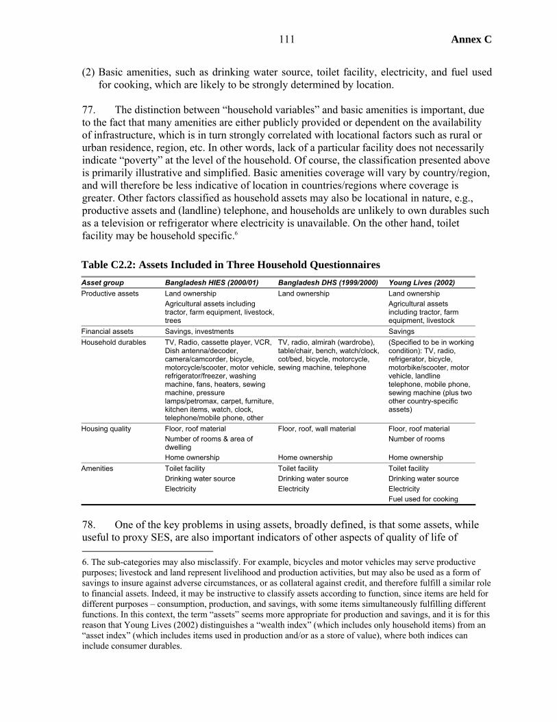
Annex C

111

(2) Basic amenities, such as drinking water source, toilet facility, electricity, and fuel used for cooking, which are likely to be strongly determined by location.

77. The distinction between “household variables” and basic amenities is important, due to the fact that many amenities are either publicly provided or dependent on the availability of infrastructure, which is in turn strongly correlated with locational factors such as rural or urban residence, region, etc. In other words, lack of a particular facility does not necessarily indicate “poverty” at the level of the household. Of course, the classification presented above is primarily illustrative and simplified. Basic amenities coverage will vary by country/region, and will therefore be less indicative of location in countries/regions where coverage is greater. Other factors classified as household assets may also be locational in nature, e.g., productive assets and (landline) telephone, and households are unlikely to own durables such as a television or refrigerator where electricity is unavailable. On the other hand, toilet facility may be household specific.6

Table C2.2: Assets Included in Three Household Questionnaires Asset group Bangladesh HIES (2000/01) Bangladesh DHS (1999/2000) Young Lives (2002) Productive assets Land ownership Land ownership Land ownership Agricultural assets including

tractor, farm equipment, livestock, trees

Agricultural assets including tractor, farm equipment, livestock

Financial assets Savings, investments Savings Household durables TV, Radio, cassette player, VCR,

Dish antenna/decoder, camera/camcorder, bicycle, motorcycle/scooter, motor vehicle, refrigerator/freezer, washing machine, fans, heaters, sewing machine, pressure lamps/petromax, carpet, furniture, kitchen items, watch, clock, telephone/mobile phone, other

TV, radio, almirah (wardrobe), table/chair, bench, watch/clock, cot/bed, bicycle, motorcycle, sewing machine, telephone

(Specified to be in working condition): TV, radio, refrigerator, bicycle, motorbike/scooter, motor vehicle, landline telephone, mobile phone, sewing machine (plus two other country-specific assets)

Housing quality Floor, roof material Floor, roof, wall material Floor, roof material Number of rooms & area of

dwelling Number of rooms

Home ownership Home ownership Home ownership Amenities Toilet facility Toilet facility Toilet facility Drinking water source Drinking water source Drinking water source Electricity Electricity Electricity Fuel used for cooking

78. One of the key problems in using assets, broadly defined, is that some assets, while useful to proxy SES, are also important indicators of other aspects of quality of life of 6. The sub-categories may also misclassify. For example, bicycles and motor vehicles may serve productive purposes; livestock and land represent livelihood and production activities, but may also be used as a form of savings to insure against adverse circumstances, or as collateral against credit, and therefore fulfill a similar role to financial assets. Indeed, it may be instructive to classify assets according to function, since items are held for different purposes – consumption, production, and savings, with some items simultaneously fulfilling different functions. In this context, the term “assets” seems more appropriate for production and savings, and it is for this reason that Young Lives (2002) distinguishes a “wealth index” (which includes only household items) from an “asset index” (which includes items used in production and/or as a store of value), where both indices can include consumer durables.

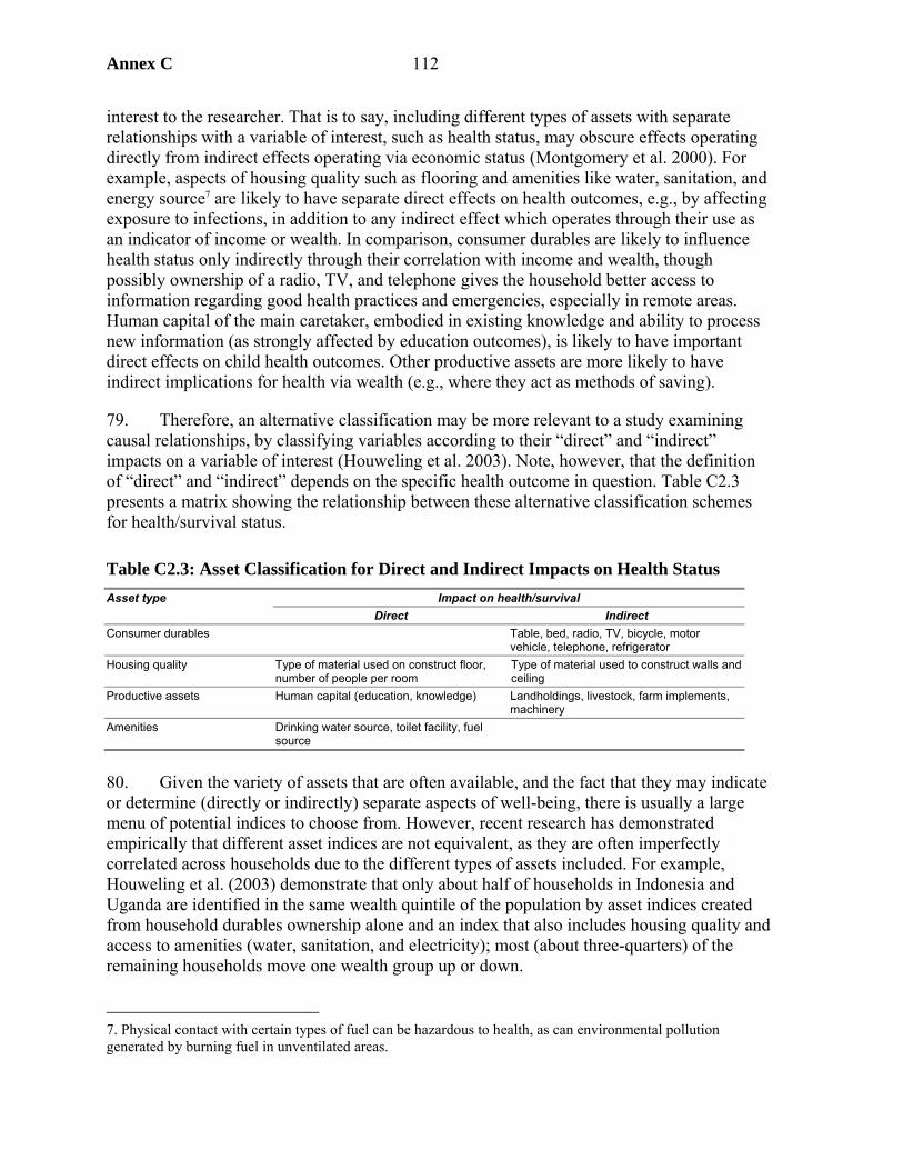
Annex C 112

interest to the researcher. That is to say, including different types of assets with separate relationships with a variable of interest, such as health status, may obscure effects operating directly from indirect effects operating via economic status (Montgomery et al. 2000). For example, aspects of housing quality such as flooring and amenities like water, sanitation, and energy source7 are likely to have separate direct effects on health outcomes, e.g., by affecting exposure to infections, in addition to any indirect effect which operates through their use as an indicator of income or wealth. In comparison, consumer durables are likely to influence health status only indirectly through their correlation with income and wealth, though possibly ownership of a radio, TV, and telephone gives the household better access to information regarding good health practices and emergencies, especially in remote areas. Human capital of the main caretaker, embodied in existing knowledge and ability to process new information (as strongly affected by education outcomes), is likely to have important direct effects on child health outcomes. Other productive assets are more likely to have indirect implications for health via wealth (e.g., where they act as methods of saving).

79. Therefore, an alternative classification may be more relevant to a study examining causal relationships, by classifying variables according to their “direct” and “indirect” impacts on a variable of interest (Houweling et al. 2003). Note, however, that the definition of “direct” and “indirect” depends on the specific health outcome in question. Table C2.3 presents a matrix showing the relationship between these alternative classification schemes for health/survival status.

Table C2.3: Asset Classification for Direct and Indirect Impacts on Health Status Impact on health/survival Asset type

Direct Indirect Consumer durables Table, bed, radio, TV, bicycle, motor

vehicle, telephone, refrigerator Housing quality Type of material used on construct floor,

number of people per room Type of material used to construct walls and ceiling

Productive assets Human capital (education, knowledge) Landholdings, livestock, farm implements, machinery

Amenities Drinking water source, toilet facility, fuel source

80. Given the variety of assets that are often available, and the fact that they may indicate or determine (directly or indirectly) separate aspects of well-being, there is usually a large menu of potential indices to choose from. However, recent research has demonstrated empirically that different asset indices are not equivalent, as they are often imperfectly correlated across households due to the different types of assets included. For example, Houweling et al. (2003) demonstrate that only about half of households in Indonesia and Uganda are identified in the same wealth quintile of the population by asset indices created from household durables ownership alone and an index that also includes housing quality and access to amenities (water, sanitation, and electricity); most (about three-quarters) of the remaining households move one wealth group up or down.

7. Physical contact with certain types of fuel can be hazardous to health, as can environmental pollution generated by burning fuel in unventilated areas.

Annex C

113

81. In sum, there are good reasons to exclude certain types of assets from an index of household socioeconomic status:

• Different types of assets represent different aspects of “wealth.” Productive assets, while representing household wealth status within livelihood groups, are unsuitable for measuring wealth between livelihood groups – for example, households that do not own cattle may not be poor, but simply do not rely on herding as a livelihood. Productive assets should therefore be excluded from the asset index. However, where productive assets represent an important aspect of wealth, such as land or livestock ownership in rural areas (or, for example, where there are limited numbers of non-productive assets, or where their distribution is highly skewed), it may be necessary to include some productive assets in order to distinguish between households. Inclusion of agricultural land may be desirable given a large rural population, despite the fact that it would also tend to mis-categorize households in urban areas as poorer than they may actually be.

• Access to certain assets will be determined by location as opposed to purchasing power of the household. Most obviously, households in rural areas are less likely to have access to amenities such as electricity, water, and sanitation, though some would not be considered poor as more conventionally defined. Therefore, amenities which are highly locational should not be used to measure household wealth. The effect of including assets determined by location is to overstate measured inequalities in household wealth. However, given that inclusion of multiple asset types as explanatory variables in regression analysis will undermine precision of estimates where the assets are strongly correlated, it may be sensible to construct separate indices for “household assets” and “amenities,” where the latter includes locational items (Houweling et al. 2003).8

• The distinction between “direct” and “indirect” determinants of a variable of interest is important. Only indicators having indirect effects (via “wealth”) on a dependent variable, say, health status, should be included as components of an index used to measure income/wealth in causal analyses. This is crucial for policy analysis because, given public resource constraints, policy may be more effective where it focuses on improving those assets that are the main drivers of change, rather than on measures to raise general wealth. The effect of including assets that have direct impacts on a variable of interest is to overstate estimated socioeconomic inequalities in that variable.9 For example, Houweling et al. (2003) estimate that inclusion of water and sanitation variables in the index augments socioeconomic inequalities in under-five mortality, in 50 percent of cases, by attributing some of the impact of these direct factors to economic status. Excluding water and sanitation from a full index that also includes consumer durables, housing quality,

8. In principle, where the locational nature of assets varies by country or within country by region, cluster-level data could be used to determine if a household potentially has access to a service (water, electricity, etc.), and the asset included in the index for those clusters with access and excluded for those without, with suitable rescaling across assets to ensure comparability across all clusters (see fn. 4).

9. In order for different SES indicators to produce different estimates of socioeconomic inequality in another variable, the indicators must produce different rankings of households and these rank differences must be correlated with the welfare outcome (Wagstaff and Watanabe 2002).

Annex C 114

and access to electricity supply, reduces inequality in under-five mortality in Chad and Malawi by more than 30 percent of the inequality index; in Brazil, Indonesia, and Pakistan, estimated inequality is reduced by between 10 and 30 percent; in Bolivia, Kenya, Tanzania, and Uganda, inequality is insignificantly affected; and in Cameroon estimated inequality rises. Excluding housing quality, water, and sanitation from the full index reduces estimated inequality by over 10 percent in 3 out of 10 (Brazil, Indonesia, and Kenya) but increases inequality in a further 3 (Chad, Malawi, and Tanzania). Additional exclusion of electricity produces estimates of inequality that are lower than the estimate produced by the full index in Bolivia, Brazil, Indonesia, Kenya, and Pakistan but higher in Chad, Malawi, and Tanzania.

82. The cost of excluding certain asset types is that it may prevent sufficiently continuous ranking of households, particularly in poor countries where ownership of durables may be highly limited among poorer segments of the population, or where the survey only collects limited information on durables.10 Houweling et al. (2003) demonstrate for DHS data that the lack of the variation in the data may necessitate inclusion of more types of assets in order to stratify poorer households evenly into wealth quintiles.

83. Including the same list of assets for different countries, and weighting these assets by the same amounts, enables comparison across countries – this is relatively easy with DHS data since the questionnaire has a standard asset list included in all surveys. However, some assets may represent household wealth to different extents across countries (or even regions/sectors within countries) and thus are not strictly comparable; e.g., bicycles do not represent the prestige in Asia, where in many countries they are relatively common and cheap, that they do in most African nations, where they are rare and expensive. Sahn and Stifel (2000) generate separate weighting schemes for 11 African countries to reflect local preferences for each asset. But by doing so they lose the ability to make inter-country comparisons. Young Lives (2002), on the other hand, uses a common weighting system across countries, though it allows for two locally specific assets for each country, and retains comparability across countries by rescaling (see fn. 4).

Determining Weighting Coefficients

84. The weightings assigned to the individual asset components of the index can be determined using a variety of methods (Filmer and Pritchett 1998). First, weights may be assumed to be equal across assets, thus the ψ in equation (1) are equal to one and the index is simply the sum of individual asset indicators. However, as Filmer and Pritchett (1998: 4) state, this method “has as its only appeal not seeming as arbitrary as it really is.” In addition, equal weighting will give the least possible categories of the asset ownership index, making it more difficult to distinguish households, which is likely to be problematic given the limited number of assets on which data are usually collected; more complex weighting systems give more thorough rankings.

10. Inherent subjectivity associated with choosing assets to be included would also tend to favor inclusion of all available assets (Gwatkin et al. 2000), though differentiation according to asset category – e.g., household assets, community assets – can limit the degree of subjectivity.

Annex C

115

85. Second, assets may be assigned unequal weights using more arbitrary, but reasonable, methods, e.g., by making reasoned choices based on other information sources. In Young Lives (2002), the wealth index is calculated as the average of three components: (1) housing quality, which is the average of number of people per room (rescaled to vary from zero to one), and dummies indicating finished floor, walls, and roof; (2) the sum of household ownership of a range of durable assets as a continuous variable scaled between zero and one; (3) the average value of dummy variables indicating access to drinking water, toilet, electricity, and cooking fuel. A particular advantage of the index is that by scaling total durables ownership between 0 and 1, it does not give undue weight to durables (of which there are more variables) over house quality and services, which an equally weighted index would.

86. Third, where data are available, weights could be determined by asset prices. Many surveys, such as the DHS, do not collect data on asset prices, though average national or regional relative prices could potentially be used instead (Young Lives 2002). However, it is not clear whether a weighting scheme based on prices is necessarily ideal – though this would create an index analogous to household income and consumption measures. Only under a highly restrictive set of assumptions do prices reflect what is measured at a theoretical level, namely marginal utilities in consumption. For example, where there exist imperfect competition, production, or consumption externalities, missing markets or imperfections in information – i.e., nearly all of the time, and especially in developing countries – prices are likely to deviate substantially from marginal utility.

87. Fourth, assets can be linearly aggregated into a single index using econometric methods. Filmer and Pritchett (1998, 1999) and Gwatkin et al. (2000) used principal components analysis (PCA) to generate asset weightings, while Sahn and Stifel (2000) used factor analysis (FA). PCA/FA are data reduction methods that examine the statistical relationships between variables.11 The first principal component/factor is the linear combination of variables explaining the maximum possible variation in the data, the second principal component/factor is that accounting for the largest of the remaining variation, etc. In analyses of asset ownership the characteristic that explains the largest variation (that estimated by the first principal component/factor) is assumed to be “wealth.” However, there are problems in attributing socioeconomic meaning to higher order components/factors, thus, only the first is used to generate the asset index. Sahn and Stifel (2000) argue that, since FA accounts for the variation in assets using a smaller number of covariates, it is therefore preferable to PCA for generating the wealth index.12 However, the methods tend to produce highly similar asset rankings.

88. There are two main concerns with PCA/FA. First, using an index may entail losing a lot of information regarding variance of asset ownership across households, but this is the case with any index. Second, PCA/FA replaces arbitrariness with statistical credibility, but does not necessarily estimate weightings that are meaningful in a socioeconomic sense – a

11. In PCA the structure of the model is determined by the variance of the data; in FA the structure is determined by the covariances (or correlations) between variables.

12. PCA has the advantage that, exclusion of higher order principal components does not theoretically result in mis-specification (omitted variables bias) in multivariate analysis, since the principal components are constructed as orthogonal to (i.e., not correlated with) one another; bias may still arise through correlation of the omitted principal component with other explanatory variables (Filmer and Pritchett 1999: 118, fn. 8).

Annex C 116

more meaningful index may be created using an “arbitrary” but reasonable weighting system, as in Young Lives (2002). In Gwatkin et al.’s (2000) index derived from PCA a household that works its own or its family’s land is assigned negative weighting, which obviously reflects location (urban residents are more likely to have access to water, sanitation, and electricity utilities – as well as, therefore, other electrical assets – but less likely to work in agriculture). However, in rural areas it is the more wealthy who own land (and the landless who are usually poorest), therefore the coefficient on land ownership, if indicating wealth, should enter positively. The negative coefficient on land is therefore a good example of why using productive assets can be misleading.

89. Another way to determine weightings econometrically is to use the coefficients estimated from a fully specified regression of the dependent variable of interest, say, height-for-age z-score, on the asset variables and all other explanatory variables (Lensink and White 2000). Given estimated coefficients, the asset index can be calculated and the regression re-estimated, replacing the individual assets with the asset index, in order for the impact of “wealth” to be determined.

90. Table C2.9 indicates some of the different ways in which assets have been aggregated in previous research. The studies were selected mainly, though not exclusively, as relating to DHS data and estimation of child mortality and nutrition. Madise et al. (1999) use indicator variables for whether the household owns any one or more than one of a set of items. Many recent studies have used an asset index similar to the one of Filmer and Pritchett (1998), which aggregates household and community-level assets into a single index. Some separate the two, e.g., Kishor and Parasuraman (1998) and Madise et al. (1999), showing that amenities (water and sanitation) have separate impact on mortality, on top of household wealth. Often, the asset index is used to categorize households into asset quintiles,13 and/or is used to calculate socioeconomic measures of health inequality.

Controlling for Household Size and Economies of Scale

91. Since data are often collected at household level, an issue arises as to whether adjustment should be made for the size and possibly composition of the household. In the case of wealth, where durable goods are used as a store of value, e.g., as insurance to be sold in the event of an adverse household shock, the size of the household determines the amount of insurance per capita a given asset can provide.14 For other household goods, such as bicycle ownership, their utility under normal conditions also implies adjustment for household size.

92. Other assets are consumed publicly by the household – i.e., economies of scale in household consumption entail that assets can be used by one member without reducing consumption possibilities for another – and therefore adjustment for household size is not

13. Wagstaff (2000) notes that deciles could be used in principle, though sample size is often too small to make this classification statistically meaningful.

14. Given whether the shock is covariate or idiosyncratic (a covariate shock inducing many households simultaneously to try to sell their assets would depress prices).

Annex C

117

necessary. Indeed, many items in the asset index can be considered public goods, although to varying degrees, e.g., consumption of some utilities such water (unless metered), electricity (for heating), aspects of housing quality such as ceiling, wall, and floor materials, some durable goods (e.g., refrigerators, radio/TV), and to a lesser extent dwelling size (until congestion is reached) (White and Masset 2003).

93. The following formula is used to adjust household-level variables for household size and economies of scale:

Ai* = Ai / n1-α (2)

where Ai* represents the adjusted value of the asset index, Ai the unadjusted index at household level, n represents the composition-adjusted number of members and α represents the scale coefficient, which ranges between 0 and 1, which represent, respectively, no economies of scale (thus the adjusted index is simply equal to the unadjusted index expressed in per capita, or per equivalent adult, terms) and indicating perfect economies of scale (household size does not alter the asset index). Empirical estimates of the scale coefficient usually are between 0.15 and 0.3 in developing countries (White and Masset 2003). For richer countries where economies of scale are likely to be greater (given the lower proportion of food in the household budget, and greater coverage of utilities) the coefficient will be higher; e.g., Wagstaff (2000) cites a study of OECD countries which implied the coefficient of scale was equal to around 0.6 (Buhmann et al. 1988).

94. Deciding on an overall scale coefficient may be problematic, given that different assets are likely to have different scale economies, which may also depend on the particular use the index is trying to capture. However, it is possible to adjust some components of the asset index selectively.

95. Most studies using an asset index (e.g., Gwatkin et al. 2000) do not indicate that they adjust the asset index for household size, which means that, implicitly, the scale coefficient is assumed to equal 0 (i.e., it is assumed that adding another person to the household does not alter the value of the index, nor the weights attached to specific variables in the index). Wagstaff (2000) takes an intermediate stance by setting the scale coefficient as equal to 0.5 for expenditure data – in his estimation for nine developing countries, assuming zero economies of scale tended to reduce socioeconomic inequalities in mortality. Filmer and Pritchett (1999) and Sahn and Stifel (2000) report that results are insensitive to different assumptions about scale coefficients.

Constructing a Wealth Index for Bangladesh

96. The preceding sections examined major conceptual and practical issues regarding the generation of an asset index. The aim is to provide recommendations for generating an asset index using DHS survey data for Bangladesh, to be used subsequently in bivariate and multivariate analyses of child mortality and nutritional outcomes. First, given the importance of separating assets which are likely to be direct determinants of health outcomes from those which have indirect effects, by representing “wealth,” the paper recommends that direct factors should be excluded, and estimated separately from wealth. Direct determinants of

Annex C 118

child nutrition and survival are drinking water source, toilet facility, and floor material of the household. This constrains which assets can be included in the index, and therefore the possibilities for differentiating between households, especially given that other items that, while having arguably less direct effects on health and nutrition, are representative of location, such as electricity, and therefore should be excluded. We are left with household durables – ownership of almirah (wardrobe), clock, cot, bicycle, radio, table, TV – and housing quality as measured by wall and roof material.15

97. A wealth index is constructed based on weightings that are both intuitive and in part determined by the variation in the data. The structure of the index follows from Young Lives (2002), in that it is the average of household durables ownership and housing quality, where total durables owned and housing quality are scaled comparably. However, unlike Young Lives (2002), which calculates all weights arbitrarily, the weightings in the index for Bangladesh for durable goods are partly chosen by the variation in the data – specifically, individual weights for each durable owned is set equal to (1-P) where P is the proportion of households owning the item; total ownership of durables is rescaled accordingly. This scheme allows much greater differentiation between households, as compared, for example, to a scheme based on equal weightings of durables.16 Weightings for housing quality are determined intuitively, though the weightings chosen are not incontrovertible, since choice of building material is partly determined by location.17 Each household’s asset score comprises the mean of:

(1) Household durables: weighted sum of dummy variables for seven goods, scaled to range between 0 and 1.18

(2) Housing quality, which is itself the mean of two components: - Wall material dummy (weight): natural/other (0), wood (0.25), tin (0.5), brick (1). - Roof material dummy (weight): natural/other (0), tin (0.5), cement/tile (1).

98. Since the weightings are time insensitive, this enables comparisons between households over time, to determine whether wealth poverty is increasing or decreasing over time. Due to the arguably strong public good aspects of the non-durables items, and given

15. It could be argued that wall and roof type have direct implications for health and nutrition – though less substantially than flooring – by increasing exposure to infection. Nevertheless, given the limited alterative assets available for the index, these variables were included in the index.

16. The weighting scheme that would maximize variance determines each score according to the variance of the asset, equal to P.(1-P), where P is the proportion owning the asset; this accords greatest weight to the assets with largest variation in ownership. This scheme was deemed unsuitable for the asset index, since it produced scores that appeared unreasonable; for example, ownership of a table and clock each received scores almost twice as large as ownership of a television.

17. In a recent field visit, it was observed that urban houses (and rural houses near main roads) were mainly constructed of corrugated metal sheets, while the main building material in rural areas were mud and thatch (Howard White, personal communication). In addition, some mud buildings were observed to be actually brick with mud daubing (which is used for traditional decorative patterns) – whereas usually enumerators fill in construction material from own observation so these houses may be misclassified.

18. Unweighted means of, or proportions of households owning, variables are as follows: radio (0.303); TV (0.137); bicycle (0.189); almirah (wardrobe) 0.265; table (0.570); clock (0.471); cot (0.787).

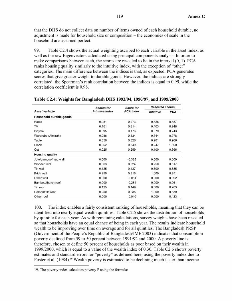
Annex C

119

that the DHS do not collect data on number of items owned of each household durable, no adjustment is made for household size or composition – the economies of scale in the household are assumed perfect.

99. Table C2.4 shows the actual weighting ascribed to each variable in the asset index, as well as the raw Eigenvectors calculated using principal components analysis. In order to make comparisons between each, the scores are rescaled to lie in the interval (0, 1). PCA ranks housing quality similarly to the intuitive index, with the exception of “other” categories. The main difference between the indices is that, as expected, PCA generates scores that give greater weight to durable goods. However, the indices are strongly correlated: the Spearman’s rank correlation between the indices is equal to 0.99, while the correlation coefficient is 0.98.

Table C2.4: Weights for Bangladesh DHS 1993/94, 1996/97, and 1999/2000 Rescaled scores

Asset variable Scores for

intuitive index Score for

PCA index Intuitive PCA Household durable goods Radio 0.081 0.273 0.326 0.887 TV 0.101 0.314 0.403 0.948 Bicycle 0.095 0.176 0.379 0.743 Wardrobe (Almirah) 0.086 0.334 0.344 0.978 Table 0.050 0.326 0.201 0.966 Clock 0.062 0.349 0.247 1.000 Cot 0.025 0.259 0.100 0.866 Housing quality Jute/bamboo/mud wall 0.000 -0.325 0.000 0.000 Wooden wall 0.063 0.024 0.250 0.517 Tin wall 0.125 0.137 0.500 0.685 Brick wall 0.250 0.316 1.000 0.951 Other wall 0.000 -0.061 0.000 0.392 Bamboo/thatch roof 0.000 -0.284 0.000 0.061 Tin roof 0.125 0.149 0.500 0.703 Cement/tile roof 0.250 0.235 1.000 0.830 Other roof 0.000 -0.040 0.000 0.423

100. The index enables a fairly consistent ranking of households, meaning that they can be identified into nearly equal wealth quintiles. Table C2.5 shows the distribution of households by quintile for each year. As with remaining calculations, survey weights have been rescaled so that households have an equal chance of being in each year. The results indicate household wealth to be improving over time on average and for all quintiles. The Bangladesh PRSP (Government of the People’s Republic of Bangladesh/IMF 2003) indicates that consumption poverty declined from 59 to 50 percent between 1991/92 and 2000. A poverty line is, therefore, chosen to define 50 percent of households as poor based on their wealth in 1999/2000, which is equal to a value of the wealth index of 0.30. Table C2.6 shows poverty estimates and standard errors for “poverty” as defined here, using the poverty index due to Foster et al. (1984).19 Wealth poverty is estimated to be declining much faster than income 19. The poverty index calculates poverty P using the formula:

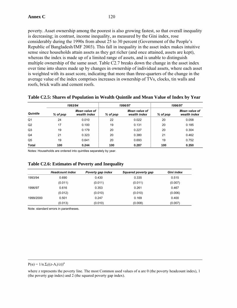
Annex C 120

poverty. Asset ownership among the poorest is also growing fastest, so that overall inequality is decreasing; in contrast, income inequality, as measured by the Gini index, rose considerably during the 1990s from about 25 to 30 percent (Government of the People’s Republic of Bangladesh/IMF 2003). This fall in inequality in the asset index makes intuitive sense since households attain assets as they get richer (and once attained, assets are kept), whereas the index is made up of a limited range of assets, and is unable to distinguish multiple ownership of the same asset. Table C2.7 breaks down the change in the asset index over time into shares made up by changes in ownership of individual assets, where each asset is weighted with its asset score, indicating that more than three-quarters of the change in the average value of the index comprises increases in ownership of TVs, clocks, tin walls and roofs, brick walls and cement roofs.

Table C2.5: Shares of Population in Wealth Quintile and Mean Value of Index by Year

1993/94 1996/97 1996/97

Quintile % of pop Mean value of wealth index % of pop

Mean value of wealth index % of pop

Mean value of wealth index

Q1 24 0.010 22 0.022 20 0.058 Q2 17 0.100 19 0.131 20 0.185 Q3 19 0.179 20 0.227 20 0.304 Q4 21 0.323 20 0.380 21 0.462 Q5 19 0.641 20 0.693 19 0.752 Total 100 0.244 100 0.287 100 0.350

Notes: Households are ordered into quintiles separately by year.

Table C2.6: Estimates of Poverty and Inequality

Headcount index Poverty gap index Squared poverty gap Gini index

1993/94 0.690 0.430 0.335 0.515 (0.011) (0.011) (0.011) (0.007) 1996/97 0.616 0.353 0.261 0.467 (0.012) (0.010) (0.010) (0.006) 1999/2000 0.501 0.247 0.169 0.400 (0.013) (0.010) (0.008) (0.007)

Note: standard errors in parantheses.

P(α) = 1/n.Σi((z-Ai)/z))α

where z represents the poverty line. The most Common used values of α are 0 (the poverty headcount index), 1 (the poverty gap index) and 2 (the squared poverty gap index).

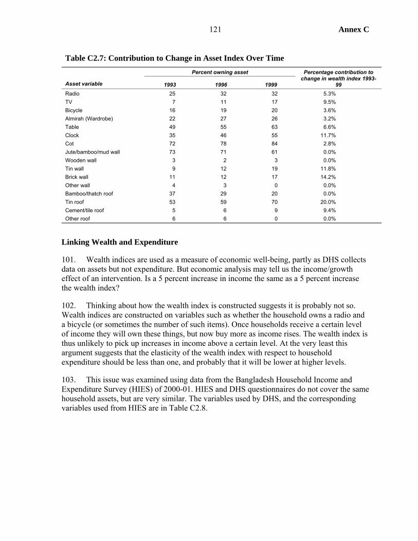
Annex C

121

Table C2.7: Contribution to Change in Asset Index Over Time Percent owning asset

Asset variable 1993 1996 1999

Percentage contribution to change in wealth index 1993-

99 Radio 25 32 32 5.3% TV 7 11 17 9.5% Bicycle 16 19 20 3.6% Almirah (Wardrobe) 22 27 26 3.2% Table 49 55 63 6.6% Clock 35 46 55 11.7% Cot 72 78 84 2.8% Jute/bamboo/mud wall 73 71 61 0.0% Wooden wall 3 2 3 0.0% Tin wall 9 12 19 11.8% Brick wall 11 12 17 14.2% Other wall 4 3 0 0.0% Bamboo/thatch roof 37 29 20 0.0% Tin roof 53 59 70 20.0% Cement/tile roof 5 6 9 9.4% Other roof 6 6 0 0.0%

Linking Wealth and Expenditure

101. Wealth indices are used as a measure of economic well-being, partly as DHS collects data on assets but not expenditure. But economic analysis may tell us the income/growth effect of an intervention. Is a 5 percent increase in income the same as a 5 percent increase the wealth index?

102. Thinking about how the wealth index is constructed suggests it is probably not so. Wealth indices are constructed on variables such as whether the household owns a radio and a bicycle (or sometimes the number of such items). Once households receive a certain level of income they will own these things, but now buy more as income rises. The wealth index is thus unlikely to pick up increases in income above a certain level. At the very least this argument suggests that the elasticity of the wealth index with respect to household expenditure should be less than one, and probably that it will be lower at higher levels.

103. This issue was examined using data from the Bangladesh Household Income and Expenditure Survey (HIES) of 2000-01. HIES and DHS questionnaires do not cover the same household assets, but are very similar. The variables used by DHS, and the corresponding variables used from HIES are in Table C2.8.

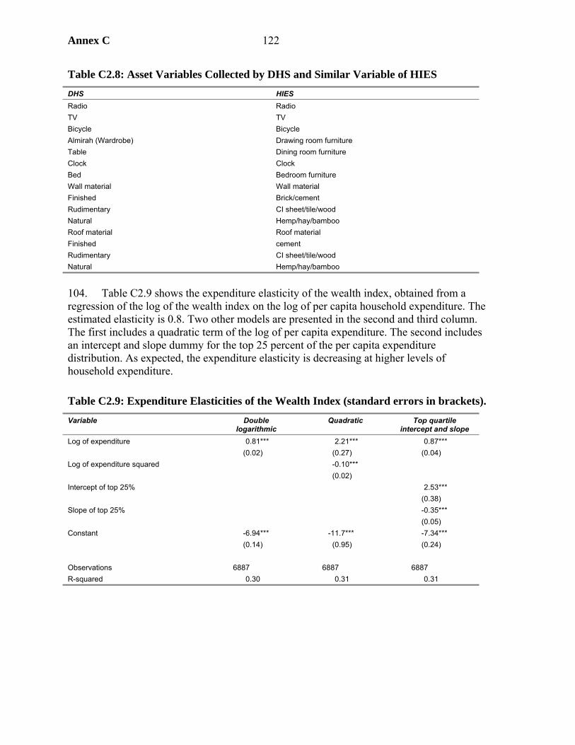
Annex C 122

Table C2.8: Asset Variables Collected by DHS and Similar Variable of HIES DHS HIES Radio Radio TV TV Bicycle Bicycle Almirah (Wardrobe) Drawing room furniture Table Dining room furniture Clock Clock Bed Bedroom furniture Wall material Wall material Finished Brick/cement Rudimentary CI sheet/tile/wood Natural Hemp/hay/bamboo Roof material Roof material Finished cement Rudimentary CI sheet/tile/wood Natural Hemp/hay/bamboo

104. Table C2.9 shows the expenditure elasticity of the wealth index, obtained from a regression of the log of the wealth index on the log of per capita household expenditure. The estimated elasticity is 0.8. Two other models are presented in the second and third column. The first includes a quadratic term of the log of per capita expenditure. The second includes an intercept and slope dummy for the top 25 percent of the per capita expenditure distribution. As expected, the expenditure elasticity is decreasing at higher levels of household expenditure.

Table C2.9: Expenditure Elasticities of the Wealth Index (standard errors in brackets). Variable Double

logarithmic Quadratic Top quartile

intercept and slope Log of expenditure 0.81***

(0.02) 2.21***

(0.27) 0.87***

(0.04) Log of expenditure squared -0.10***

(0.02)

Intercept of top 25% 2.53*** (0.38)

Slope of top 25% -0.35*** (0.05)

Constant -6.94*** (0.14)

-11.7*** (0.95)

-7.34*** (0.24)

Observations 6887 6887 6887 R-squared 0.30 0.31 0.31

Annex C

123

Figure C2.1: Plot of the Predicted Values Against Per-Capita Expenditure from the 3 Models Above

-4

-3-2

-10

1

0 5000 10000 15000Monthly per capita hhold csm

log-linear quadratictop 25%

Annex C 124

Table C2.8: Asset Score for Bangladesh DHS 1996/97, Generated by Principal Components Analysis as Reported in Gwatkin et al. (2000)

Household score if: Ownership (1=yes,

0=no) Asset score

Asset variable Asset factor

scores has

asset does not have

asset Household

A Household

B Household

A Household

B Has electricity 0.118 0.214 -0.065 1 0 0.214 -0.065 Has radio 0.071 0.104 -0.049 1 1 0.104 0.104 Has television 0.125 0.347 -0.045 1 0 0.347 -0.045 Has bicycle 0.032 0.065 -0.016 1 1 0.065 0.065 If household works own or family’s agric. land -0.022 -0.042 0.012 0 1 0.012 -0.042 If piped drinking water in residence 0.104 0.526 -0.021 0 0 -0.021 -0.021 If piped drinking water outside residence 0.020 0.179 -0.002 1 0 0.179 -0.002 If has tubewell for drinking water -0.063 -0.022 0.186 0 0 0.186 0.186 If has a surface well -0.009 -0.066 0.001 0 1 0.001 -0.066 If rain for drinking water -0.001 -0.023 0.000 0 0 0.000 0.000 If uses river, canal or surface water for drinking -0.009 -0.049 0.002 0 0 0.002 0.002 Other source of drinking water 0.000 0.005 0.000 0 0 0.000 0.000 If uses septic tank or toilet 0.127 0.370 -0.043 1 0 0.370 -0.043 If has pit latrine -0.016 -0.041 0.006 0 1 0.006 -0.041 If uses a water-sealed or slab latrine 0.017 0.033 -0.009 0 0 -0.009 -0.009 If has open latrine -0.033 -0.059 0.019 0 0 0.019 0.019 If uses a hanging latrine -0.012 -0.054 0.003 0 0 0.003 0.003 If uses bush, field as latrine -0.054 -0.092 0.031 0 0 0.031 0.031 If has other type of latrine -0.001 -0.031 0.000 0 0 0.000 0.000 If has earth or bamboo as principal floor in dwelling -0.152 -0.057 0.401 0 0 0.401 0.401 If has wood, plank principal floor in dwelling 0.010 0.146 -0.001 0 1 -0.001 0.146 If has cement principal floor 0.153 0.415 -0.056 1 0 0.415 -0.056 If has other type of flooring 0.003 0.135 0.000 0 0 0.000 0.000 If has cane, palm, trunks for walls -0.108 -0.074 0.158 0 0 0.158 0.158 If has rudimentary walls -0.004 -0.021 0.001 0 1 0.001 -0.021 If has tin for walls 0.012 0.034 -0.004 0 0 -0.004 -0.004 If has bricks, cement blocks, concrete walls 0.143 0.361 -0.057 1 0 0.361 -0.057 If has other material for walls -0.010 -0.054 0.002 0 0 0.002 0.002 If has natural material roofing -0.061 -0.095 0.039 0 0 0.039 0.039 If has rudimentary roofing 0.003 0.003 -0.004 0 1 -0.004 0.003 If has finished roof 0.125 0.498 -0.031 1 0 0.498 -0.031 If has other roofing -0.014 -0.053 0.004 0 0 0.004 0.004 Total asset score 3.379 0.659

125 Annex C

Table C2.9: Studies Using Assets to Measure SES Asset type

Author Description of study Country

Asset/income measure

Household consumer durables

Household dwelling characteristics Amenities

Non-housing (production) items

Hill et al. (1996)

Child mortality, DHS

Kenya Asset index (PCA), generating wealth quintiles

Radio, TV, Refrigerator, Bicycle, Motorbike, car

Quality of floor, roof

Electricity

Filmer and Pritchett (1998)

Educational enrolment, NFHS

Indian states

Asset index (PCA), generating wealth quintiles

Clock/watch, bicycle, radio, TV, sewing machine, refrigerator, car, motorcycle.

Number of rooms, building materials, cooking source

Toilet facilities, drinking water, electric lighting

HH owns more than 6 acres of land

Filmer and Pritchett (1999)

Educational attainment, DHS

33 countries across the world, including Bangladesh

Asset index (PCA), generating wealth quintiles

Clock/watch, bicycle, radio, TV, sewing machine, refrigerator, car, motorcycle.

Number of rooms, building materials, cooking source

Toilet facilities, drinking water, electric lighting

HH owns more than 6 acres of land

Gage et al. (1996)

Immunization and Diarrhea, DHS

11 sub-Saharan African countries

Asset index (asset dummies summed – equal weightings)

Radio, motorcycle, car

Non-mud floor Some toilet facility, piped drinking water, electricity

Gwatkin et al. (2000)

Health, nutrition and population, DHS

Bangladesh Asset index (PCA), generating wealth quintiles

Radio, TV, bicycle Floor material, wall material, roof material

Toilet facilities, drinking water, electricity

HH works own or family’s agric. Land

Kishor and Parasuraman (1998)

Infant and child mortality, NFHS

India HH asset index (ownership dummies summed – weights chosen apparently subjectively), toilet and water facilities index (ranges from 0-2)

Asset (weight in parentheses): clock (1), sewing machine (2), sofa (2), fan (2), radio (2), bicycle (2), refrigerator (3), TV (3), scooter (3), car (4).

No toilet or water, either toilet or water, both toilet and water.

Madise et al. (1999)

Nutrition, DHS

6 in sub-Saharan Africa

Asset dummies: variables for hh items (at least one item, two or more items) and community items entered separately

‘Modern hh items’: working radio, TV, bicycle, motorcycle, car

Floor material, wall material

Electricity, pit/bucket toilet, flush toilet

Masset and White (2002)

Infant and child mortality, NFHS

India HH asset index – non-weighted, scaled to one

Radio, TV set, refrigerator, bicycle, motorcycle, car, land, livestock, clock and sewing machine.

Sahn and Stifel (2000)

‘Poverty’ across countries and time

11 in sub-Saharan Africa

Asset index (FA) Radio, TV, refrigerator, bicycle, car, motorcycle

Floor quality Toilet facilities, drinking water

Years of education of household head (or indicator variable where years education is not available)

Annex C 126

Table C2.9: Studies Using Assets to Measure SES Asset type

Author Description of study Country

Asset/income measure

Household consumer durables

Household dwelling characteristics Amenities

Non-housing (production) items

Sastry (1996) Child mortality, DHS variant.

Brazil Asset dummies measured at community level (proportions per population) (hh level SES measured using hh income)

Water supply, sanitation, electricity, garbage collection/public cleaning service (also health facilities and education per population and num TV stations)

Wagstaff and Watanabe (2002)

Nutrition, LSMS

19 countries Income, asset index (PCA)

Radio, refrigerator, TV, motorcycle

Rooms per person, floor quality

Water supply, sanitation

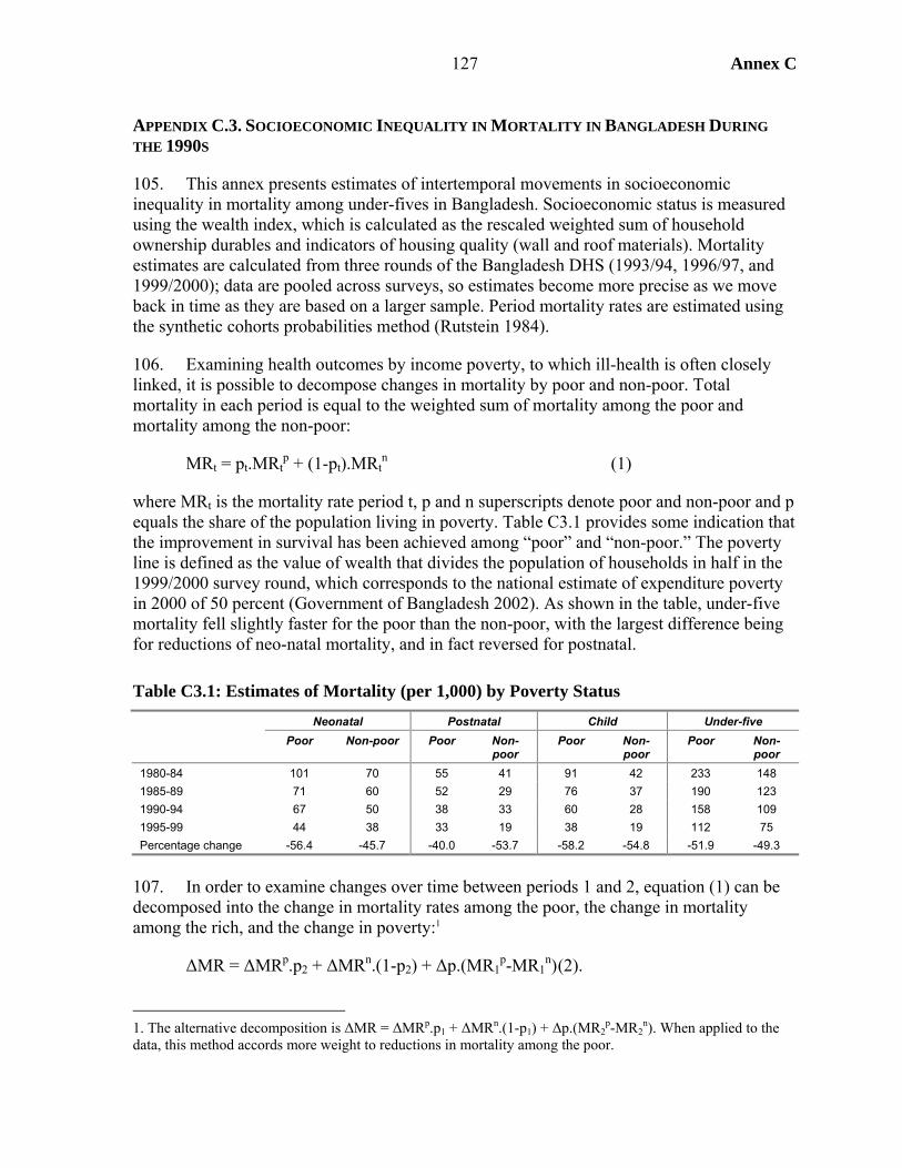
Annex C

127

APPENDIX C.3. SOCIOECONOMIC INEQUALITY IN MORTALITY IN BANGLADESH DURING THE 1990S

105. This annex presents estimates of intertemporal movements in socioeconomic inequality in mortality among under-fives in Bangladesh. Socioeconomic status is measured using the wealth index, which is calculated as the rescaled weighted sum of household ownership durables and indicators of housing quality (wall and roof materials). Mortality estimates are calculated from three rounds of the Bangladesh DHS (1993/94, 1996/97, and 1999/2000); data are pooled across surveys, so estimates become more precise as we move back in time as they are based on a larger sample. Period mortality rates are estimated using the synthetic cohorts probabilities method (Rutstein 1984).

106. Examining health outcomes by income poverty, to which ill-health is often closely linked, it is possible to decompose changes in mortality by poor and non-poor. Total mortality in each period is equal to the weighted sum of mortality among the poor and mortality among the non-poor:

MRt = pt.MRtp + (1-pt).MRt

n (1)

where MRt is the mortality rate period t, p and n superscripts denote poor and non-poor and p equals the share of the population living in poverty. Table C3.1 provides some indication that the improvement in survival has been achieved among “poor” and “non-poor.” The poverty line is defined as the value of wealth that divides the population of households in half in the 1999/2000 survey round, which corresponds to the national estimate of expenditure poverty in 2000 of 50 percent (Government of Bangladesh 2002). As shown in the table, under-five mortality fell slightly faster for the poor than the non-poor, with the largest difference being for reductions of neo-natal mortality, and in fact reversed for postnatal.

Table C3.1: Estimates of Mortality (per 1,000) by Poverty Status Neonatal Postnatal Child Under-five Poor Non-poor Poor Non-

poor Poor Non-

poor Poor Non-

poor 1980-84 101 70 55 41 91 42 233 148 1985-89 71 60 52 29 76 37 190 123 1990-94 67 50 38 33 60 28 158 109 1995-99 44 38 33 19 38 19 112 75 Percentage change -56.4 -45.7 -40.0 -53.7 -58.2 -54.8 -51.9 -49.3

107. In order to examine changes over time between periods 1 and 2, equation (1) can be decomposed into the change in mortality rates among the poor, the change in mortality among the rich, and the change in poverty:1

ΔMR = ΔMRp.p2 + ΔMRn.(1-p2) + Δp.(MR1p-MR1

n) (2).

1. The alternative decomposition is ΔMR = ΔMRp.p1 + ΔMRn.(1-p1) + Δp.(MR2

p-MR2n). When applied to the

data, this method accords more weight to reductions in mortality among the poor.

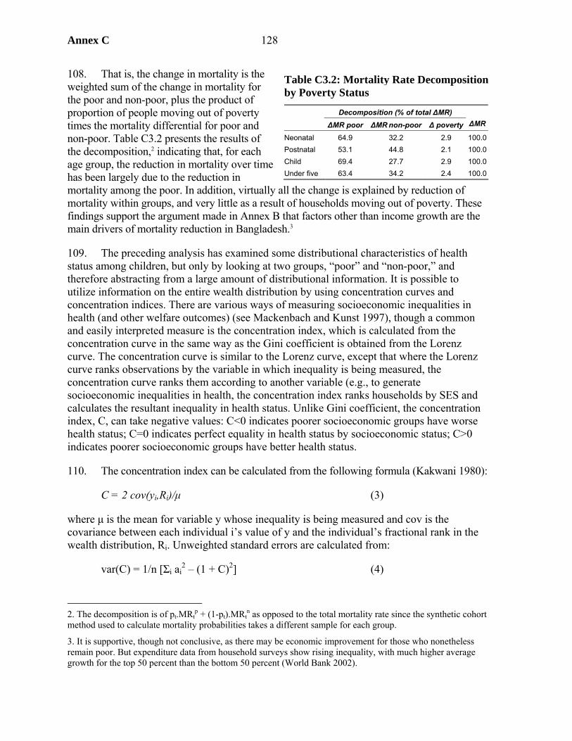
Annex C 128

108. That is, the change in mortality is the weighted sum of the change in mortality for the poor and non-poor, plus the product of proportion of people moving out of poverty times the mortality differential for poor and non-poor. Table C3.2 presents the results of the decomposition,2 indicating that, for each age group, the reduction in mortality over time has been largely due to the reduction in mortality among the poor. In addition, virtually all the change is explained by reduction of mortality within groups, and very little as a result of households moving out of poverty. These findings support the argument made in Annex B that factors other than income growth are the main drivers of mortality reduction in Bangladesh.3

109. The preceding analysis has examined some distributional characteristics of health status among children, but only by looking at two groups, “poor” and “non-poor,” and therefore abstracting from a large amount of distributional information. It is possible to utilize information on the entire wealth distribution by using concentration curves and concentration indices. There are various ways of measuring socioeconomic inequalities in health (and other welfare outcomes) (see Mackenbach and Kunst 1997), though a common and easily interpreted measure is the concentration index, which is calculated from the concentration curve in the same way as the Gini coefficient is obtained from the Lorenz curve. The concentration curve is similar to the Lorenz curve, except that where the Lorenz curve ranks observations by the variable in which inequality is being measured, the concentration curve ranks them according to another variable (e.g., to generate socioeconomic inequalities in health, the concentration index ranks households by SES and calculates the resultant inequality in health status. Unlike Gini coefficient, the concentration index, C, can take negative values: C<0 indicates poorer socioeconomic groups have worse health status; C=0 indicates perfect equality in health status by socioeconomic status; C>0 indicates poorer socioeconomic groups have better health status.

110. The concentration index can be calculated from the following formula (Kakwani 1980):

C = 2 cov(yi,Ri)/μ (3)

where μ is the mean for variable y whose inequality is being measured and cov is the covariance between each individual i’s value of y and the individual’s fractional rank in the wealth distribution, Ri. Unweighted standard errors are calculated from:

var(C) = 1/n [Σi ai2 – (1 + C)2] (4)

2. The decomposition is of pt.MRt

p + (1-pt).MRtn as opposed to the total mortality rate since the synthetic cohort

method used to calculate mortality probabilities takes a different sample for each group.

3. It is supportive, though not conclusive, as there may be economic improvement for those who nonetheless remain poor. But expenditure data from household surveys show rising inequality, with much higher average growth for the top 50 percent than the bottom 50 percent (World Bank 2002).

Table C3.2: Mortality Rate Decomposition by Poverty Status

Decomposition (% of total ΔMR) ΔMR poor ΔMR non-poor Δ poverty ΔMR

Neonatal 64.9 32.2 2.9 100.0Postnatal 53.1 44.8 2.1 100.0Child 69.4 27.7 2.9 100.0Under five 63.4 34.2 2.4 100.0

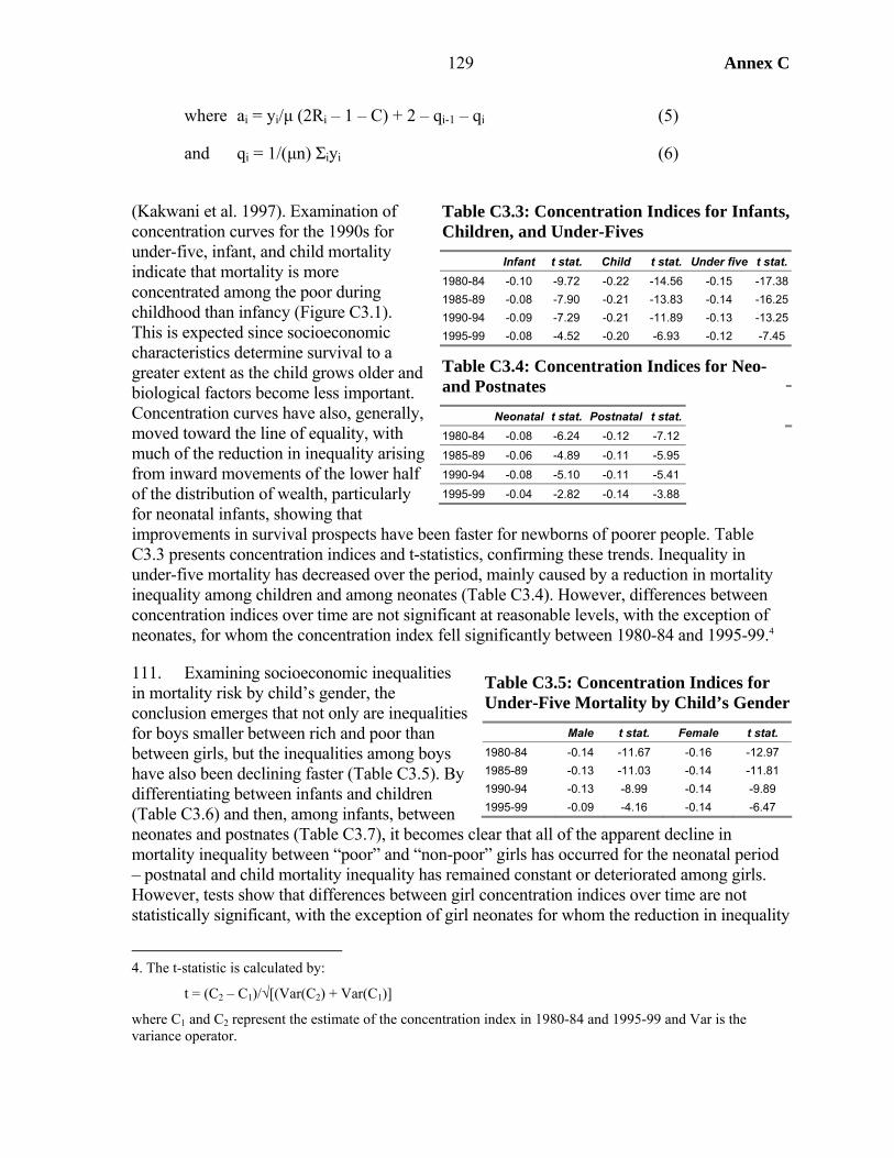
Annex C

129

where ai = yi/μ (2Ri – 1 – C) + 2 – qi-1 – qi (5)

and qi = 1/(μn) Σiyi (6)

(Kakwani et al. 1997). Examination of concentration curves for the 1990s for under-five, infant, and child mortality indicate that mortality is more concentrated among the poor during childhood than infancy (Figure C3.1). This is expected since socioeconomic characteristics determine survival to a greater extent as the child grows older and biological factors become less important. Concentration curves have also, generally, moved toward the line of equality, with much of the reduction in inequality arising from inward movements of the lower half of the distribution of wealth, particularly for neonatal infants, showing that improvements in survival prospects have been faster for newborns of poorer people. Table C3.3 presents concentration indices and t-statistics, confirming these trends. Inequality in under-five mortality has decreased over the period, mainly caused by a reduction in mortality inequality among children and among neonates (Table C3.4). However, differences between concentration indices over time are not significant at reasonable levels, with the exception of neonates, for whom the concentration index fell significantly between 1980-84 and 1995-99.4

111. Examining socioeconomic inequalities in mortality risk by child’s gender, the conclusion emerges that not only are inequalities for boys smaller between rich and poor than between girls, but the inequalities among boys have also been declining faster (Table C3.5). By differentiating between infants and children (Table C3.6) and then, among infants, between neonates and postnates (Table C3.7), it becomes clear that all of the apparent decline in mortality inequality between “poor” and “non-poor” girls has occurred for the neonatal period – postnatal and child mortality inequality has remained constant or deteriorated among girls. However, tests show that differences between girl concentration indices over time are not statistically significant, with the exception of girl neonates for whom the reduction in inequality

4. The t-statistic is calculated by:

t = (C2 – C1)/√[(Var(C2) + Var(C1)]

where C1 and C2 represent the estimate of the concentration index in 1980-84 and 1995-99 and Var is the variance operator.

Table C3.3: Concentration Indices for Infants, Children, and Under-Fives Infant t stat. Child t stat. Under five t stat.1980-84 -0.10 -9.72 -0.22 -14.56 -0.15 -17.381985-89 -0.08 -7.90 -0.21 -13.83 -0.14 -16.251990-94 -0.09 -7.29 -0.21 -11.89 -0.13 -13.251995-99 -0.08 -4.52 -0.20 -6.93 -0.12 -7.45

Table C3.4: Concentration Indices for Neo- and Postnates Neonatal t stat. Postnatal t stat. 1980-84 -0.08 -6.24 -0.12 -7.12 1985-89 -0.06 -4.89 -0.11 -5.95 1990-94 -0.08 -5.10 -0.11 -5.41 1995-99 -0.04 -2.82 -0.14 -3.88

Table C3.5: Concentration Indices for Under-Five Mortality by Child’s Gender Male t stat. Female t stat. 1980-84 -0.14 -11.67 -0.16 -12.97 1985-89 -0.13 -11.03 -0.14 -11.81 1990-94 -0.13 -8.99 -0.14 -9.89 1995-99 -0.09 -4.16 -0.14 -6.47

Annex C 130

in mortality risk between 1980-84 and 1995-99 is marginally significant at the 10 percent level. For boys, much of the decline in socioeconomic inequality in mortality occurred for children and, to a lesser extent, for neonates, while inequalities in postnatal mortality widened during the mid-1990s, though none of these differences are statistically significant.

Table C3.6: Concentration Indices by Child’s Gender Infant Child Male t stat. Female t stat. Male t stat. Female t stat. 1980-84 -0.09 -7.00 -0.11 -6.63 -0.20 -8.69 -0.23 -11.51 1985-89 -0.10 -6.77 -0.05 -4.16 -0.18 -7.95 -0.23 -11.44 1990-94 -0.10 -5.63 -0.07 -4.55 -0.18 -6.90 -0.22 -9.89 1995-99 -0.08 -3.12 -0.08 -3.29 -0.15 -3.52 -0.24 -6.16

Table C3.7: Concentration Indices by Child’s Gender Neonatal Postnatal Male t stat. Female t stat. Male t stat. Female t stat. 1980-84 -0.09 -4.83 -0.08 -3.96 -0.10 -4.83 -0.15 -5.23 1985-89 -0.07 -4.14 -0.04 -2.60 -0.14 -5.27 -0.07 -3.07 1990-94 -0.07 -3.74 -0.08 -3.43 -0.15 -4.48 -0.08 -3.13 1995-99 -0.06 -2.58 -0.03 -1.52 -0.12 -2.03 -0.17 -3.71

112. It is possible to decompose socioeconomic inequalities in mortality risk into inequalities in the determinants of mortality; similarly changes in inequalities can be decomposed into changes in inequality of the determinants.

113. Following Wagstaff (2000), the concentration index can be expressed as the weighted sum of the concentration indices ci of the n variables determining mortality:

C* = y1c1 + y2c2 + … + yncn (7)

where the weights are calculated by multiplying the coefficient estimate by the mean of that variable and dividing by the linear prediction of the regression model at the means of the data. Note that what is really being examined in this analysis is socioeconomic inequality in the underlying latent variable in the case of probit regressions (for neonatal and postnatal mortality) and the log of the hazard ratio in the case of the survival model (for child mortality). The change in the concentration index over time t can also be decomposed into the proportional contribution of the change in concentration indices for each variable i:

Δ = y(Δci)/C* (8)

Annex C

131

114. Table C3.8 presents a summary of the decomposition of the changes in concentration indices over time for determinants of mortality used in subsequent regressions, with the full results, including concentration indices for each variable, given in Table C3.9. Socioeconomic inequalities in determinants of mortality have generally declined over time; this is true for factors such as wealth, education attainment, and maternal mobility. It is not true for the measures of health: there has been no change for antenatal care and a worsening for vitamin A and having no vaccination. For neonatal mortality, fertility-related changes, such as birth order have played the largest role, followed by a reduction in the inequality in access to electricity. The decompositions for postnatal mortality are unrevealing, due to the small estimated change in postnatal mortality during the period. Finally, for children the most important single variable contributing to reduction in socioeconomic inequality in mortality is wealth, followed by maternal education, which accounts for just over half the change accounted for by wealth.

Table C3.8: Summary of Contribution to Changes in Concentration Index

Neonatal Postnatal Child

Wealth 0.012 0.001 -0.164

Education -0.019 0.002 -0.085

Fertility related -0.149 -0.017 0.023

Electricity -0.069 0.000 0.005

Water and sanitation -0.015 0.000 0.003

Gender related -0.014 -0.001 0.061

Locational -0.003 -0.004 0.010

Other 0.121 0.001 0.060

Total -0.136 -0.018 -0.087

Annex C 132

Table C3.9: Decomposition of Changes in Socioeconomic Inequality in Mortality by Age Group Concentration index C Contribution to change in C for mortality Early-90s Late-90s Neonatal Postnatal Child Wealth 0.514 0.412 0.012 0.001 -0.164 Electricity 0.593 0.478 -0.069 0.000 0.005 Water & Sanitation 0.899 0.846 -0.015 0.000 0.003 Mother Primary Ed 0.030 -0.049 -0.011 0.000 -0.048 Mother Finished Primary 0.313 0.182 -0.027 0.000 -0.011 Mother Secondary Ed 0.552 0.425 0.025 0.001 -0.025 Mother Fin Second Or Higher 0.763 0.741 -0.006 0.001 -0.001 Contraception 0.041 0.037 -0.020 -0.001 -0.003 Multiple Birth 0.112 -0.087 0.102 0.000 Age At Birth -0.002 -0.003 -0.027 -0.001 -0.004 Age At Birth Sq -0.004 -0.008 0.042 Prev Child Died -0.126 -0.117 -0.005 0.000 -0.001 Prec Interval <15 0.004 -0.064 0.043 0.000 Prev Child Died X Prec Interval -0.011 -0.128 -0.028 0.000 Birth Order -0.034 -0.058 -0.398 -0.009 0.030 Birth Order Sq -0.048 -0.097 0.297 -0.006 Female Child -0.008 -0.005 0.004 0.000 0.004 Female X Birth Order -0.036 -0.066 0.000 0.052 Female Head Of Hh 0.003 0.004 0.002 0.000 0.000 Mother’s Mobility 0.026 0.017 -0.015 0.000 -0.001 Mother Divorced -0.258 -0.083 0.001 0.000 -0.004 Mother Remarried -0.009 -0.016 -0.006 -0.001 0.010 Antenatal Visits 0.304 0.304 -0.001 Chittagong 0.010 -0.026 -0.011 0.000 -0.017 Dhaka 0.058 0.069 0.003 0.000 0.007 Khulna -0.046 0.104 0.035 0.001 0.059 Rajshahi -0.062 -0.107 -0.009 -0.001 -0.033 Rural -0.048 -0.073 -0.021 -0.004 -0.006 Born In Feb-Mar X Rural -0.082 -0.065 0.004 0.000 Born In Apr-May X Rural -0.029 -0.083 -0.029 0.000 Born In Jun-Jul X Rural -0.064 -0.037 0.003 0.000 Born In Aug-Sep X Rural -0.069 -0.076 -0.003 0.000 Born In Oct-Nov X Rural -0.053 -0.099 -0.008 0.000 Mean_Vitamin A 0.005 0.076 0.001 0.037 Mean_No_Vaccine -0.035 -0.086 0.024

133 Annex C

Figure C3.1: Concentration Curves for Infants, Children, and Under-Fives, all Children and by Gender

0.2

.4.6

.81

Cum

. pro

p. d

eath

s

0 .2 .4 .6 .8 1Cum. prop. live births

Late 90s 45 degree lineEarly 90s

Concentration curves for under-5 mortality

0.2

.4.6

.81

Cum

. pro

p. d

eath

s



Concentration curves for neonatal mortality

0.2

.4.6

.81

Cum

. pro

p. d

eath

s



Concentration curves for child mortality(Children aged 12-59 mos.)

0.2

.4.6

.81

Cum

. pro

p. d

eath

s



Concentration curves for postnatal mortality

0.2

.4.6

.81

Cum

. pro

p. d

eath

s



Concentration curves for infant mortality

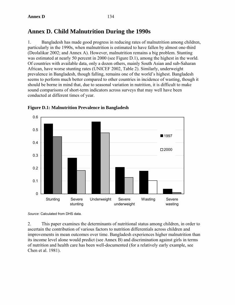
Annex D 134

Annex D. Child Malnutrition During the 1990s

1. Bangladesh has made good progress in reducing rates of malnutrition among children, particularly in the 1990s, when malnutrition is estimated to have fallen by almost one-third (Deolalikar 2002; and Annex A). However, malnutrition remains a big problem. Stunting was estimated at nearly 50 percent in 2000 (see Figure D.1), among the highest in the world. Of countries with available data, only a dozen others, mainly South Asian and sub-Saharan African, have worse stunting rates (UNICEF 2002, Table 2). Similarly, underweight prevalence in Bangladesh, though falling, remains one of the world’s highest. Bangladesh seems to perform much better compared to other countries in incidence of wasting, though it should be borne in mind that, due to seasonal variation in nutrition, it is difficult to make sound comparisons of short-term indicators across surveys that may well have been conducted at different times of year.

Figure D.1: Malnutrition Prevalence in Bangladesh

Source: Calculated from DHS data. 2. This paper examines the determinants of nutritional status among children, in order to ascertain the contribution of various factors to nutrition differentials across children and improvements in mean outcomes over time. Bangladesh experiences higher malnutrition than its income level alone would predict (see Annex B) and discrimination against girls in terms of nutrition and health care has been well-documented (for a relatively early example, see Chen et al. 1981).

0

0.1

0.2

0.3

0.4

0.5

0.6

Stunting Severestunting

Underweight Severeunderweight

Wasting Severewasting

1997

2000

135 Annex D

Modeling Child Nutritional Status

3. Nutritional status is measured anthropometrically,1 using three indicators: height for age (stunting), weight for height (wasting), and weight for age (underweight). Height for age is an indicator of long-term malnutrition because it measures nutrition cumulatively over time. Weight for height is sensitive to short-term fluctuations in nutritional state. Weight for age is a composite measure of weight for height and height for age; it is criticized due to its inability to distinguish children who are truly thin from those who weigh less because they are shorter. However, it has been shown to be more closely related to mortality risk in Bangladesh than other indicators (Chen et al. 1980).2

4. Child nutritional status is determined by comparing the anthropometric indicator for each child in the survey population to the expected measurement for a child of the same age/height and sex from a healthy reference population.3 This comparison can be done in a variety of ways, the most effective of which is to normalize the anthropometric measure by calculating z scores:

),(

),(),(

gy

gyigyi

xz

σμ−

=

where xi indicates the anthropometric measure for individual i and μ and σ are the respective median and standard deviation of the anthropometric measure for the appropriate age or height y and gender g in the reference population.4

5. The basic model of child nutritional status is due to UNICEF (1990), in which nutrition depends proximately on dietary intake and health status. Thus, high rates of child malnutrition are likely to be closely linked to the underlying household food insecurity and the exposure to infectious disease such as diarrhea, due to poor sanitary environment and inadequate medical treatment. A third underlying factor is the quantity and quality of child care, which determines how effectively income is converted into nutrition and the share allocated to children (and, importantly, which children receive the most), as well as the healthiness of the home and community environments. Note that these three underlying factors may be complements or substitutes in the production of child health.

6. The meta-analysis conducted as a background paper for this study (Charmarbagwala et al. 2004) provides a summary of the literature modeling nutritional status, as indicated by

1. Anthropometry measures the body’s quantitative change in response to changes in the balance between net energy requirements and net energy intake from food.

2. According to Chen et al (1980), in a longitudinal study, weight for age was found to be the strongest predictor of mortality, followed by height for age and finally weight for height. Of course, short children may well be more at risk where height indicates low birth weight or a history of sickness.

3. The reference population is the NCHS/WHO (1978) reference.

4. Z scores are preferable to other measures, such as the percentage of the reference median, because they account for distributional variation specific to different ages or heights in the reference population. Children with z scores between -2 and -3 are chronically malnourished and those below -3 z scores severely malnourished.

Annex D 136

height for age z score. In multivariate analysis, nutritional status can be modeled as a function of child-specific factors, d, household-specific factors, h, and community factors, e:

z = n(d, h, e).

7. Child-specific factors include demographic variables such as child’s age, gender, birth order and birth interval, and behavioral factors such as breastfeeding and immunization. The relationship between age and nutritional status depends on whether the anthropometric indicator measures short-term or long-term malnutrition. For short-term measures, age should exert a non-linear concave impact on nutritional status: nutrition deteriorates in the period in which children are most susceptible to disease – from the onset of weaning (which should be at age 6 months) until age 24 months – and improves thereafter. For long-term measures the relationship between age and malnutrition is also likely to be concave, though because stunting is often permanent, the function is unlikely to fall after 24 months of age. Gender-based discrimination in South Asia means that the coefficient on a female dummy may be negative; girls who have older sisters or who are competing with the first-born male are particularly likely to be discriminated against (Croll 2001).5 Surprisingly, the meta-analysis found that boy children were significantly more likely to be malnourished than girls (Charmarbagwala et al. 2004). However, this finding may be due to mortality selectivity, which was not allowed for in previous studies (see below).

8. More generally, children of high birth order (born latest) and children born closely together are more likely to have lower nutritional states, due to socioeconomic factors (resource competition) and biological factors (e.g., physically depleted mothers may give birth to low birth-weight babies and may be unable to breastfeed). Mozumder et al (2000) find that short subsequent birth interval impacts negatively on weight for age, but no statistically significant impact of preceding interval, which they attribute to the likelihood that “the new infant holds and advantageous position with the mother, compared with any older siblings, because of breast-feeding” (p. 295). One issue concerning use of household composition and demographic variables is that they may be endogenous to decisions on child health, leading to biased regression estimates. As Horton (1986) argues, parents are likely to make joint decisions on child quantity and child quality (demonstrated, for example, by nutritional status). Regression estimation should account for this source of bias, e.g., through use of instruments or by dropping endogenous demographic variables to assess robustness of the other coefficient estimates.

9. Child immunization is an important variable to control for – vaccination reduces chances of contracting debilitating disease. A mother’s decision to immunize her child depends partly on availability health services and income, but also her preference regarding modern medical care, which is unobservable.6 Due to unobservable heterogeneity, behavioral variables such as immunization may be correlated with the error term in the regression equation, leading to biased regression estimates (Rosenzweig and Schultz 1983; Thomas et 5. Using multivariate analysis of panel data, Bairagi (1986) finds evidence that nutrition discrimination against girls increases following famine.

6. Controlling for education and health knowledge in the regression equation should proxy some component of this heterogeneity.

137 Annex D

al. 1991; Alderman and Garcia 1994). Consistent estimation requires use of instrumental variables (the “production function” approach).

10. In addition to the above, determinants of long-term malnutrition (height for age) should control for genetic health endowment and birth weight, which can be an important determinant of ill-health and height throughout childhood and onwards. Commonly used indicators of health endowment are (log of) mother’s height and, due to seasonal variation in food availability, month of birth may be a good proxy for birth weight; DHS round 2000 also provides data on mother’s recollection of low birth weight.

11. Household-specific factors include parental or family resources such as income, household size and composition, parental education, mother’s age and mobility, and sex of the household head; these are proxies for food security and the quality and quantity of care provided to children.

12. Income – broadly defined to include imputed own production – is a key determinant of household nutritional intake. In the health production function literature, income is considered jointly determined with nutrition and health, leading to biased estimates of the coefficient on the income variable in standard regression analysis (see Annex C). The extent to which current income and child health are endogenously determined can be questioned for extreme cases such as long-term malnutrition (stunting) and mortality (see Charmarbagwala et al. 2004). However, estimation techniques usually instrument for income, a suitable instrumental variable being wealth.7 The meta-analysis found income/wealth to be strongly correlated with child nutrition, with the clear majority of studies finding a significantly positive effect (ibid.).

13. Food availability is highly seasonally dependent in rural areas of Bangladesh (see Annex J). Models of short-term nutritional status should therefore include the month that measurement was taken (interacted with a rural sector dummy). The wet season in July-October, which occurs before the main rice harvest, aman, is a critical time of year for child health, due to greater prevalence of water-borne disease (diarrhea, malaria) and food scarcity (Muhuri 1996; and Annex I). DHS data were collected between November and March, limiting the possibilities to explore seasonal variation in short-term malnutrition to this 5-month period. DHS 2000 round do, however, provide data on the household’s (self-reported) food availability during the year.

14. Household size is likely to be positively correlated with child nutrition, reflecting availability of replacement caretakers, including older children and grandparents (people who may otherwise be considered economic “dependents”). The meta-analysis found evidence for a significantly positive effect of household size on nutrition, and a significantly negative effect of presence of young children in the household (Charmarbagwala et al. 2004). Estimation should account for potential endogeneity of household composition and demographic variables, as explicated above.

7. The wealth index is calculated as the weighted sum of household durable goods ownership and quality of housing (wall and roof) building materials. This excludes factors that are expected to have “direct” effects on child health and nutrition, such as drinking water source, sanitation, and dwelling flooring, in order that these effects can be estimated separately.

Annex D 138

15. Maternal education usually has a positive effect on child nutrition, as indicated by the meta-analysis, which found education to be positively correlated with child nutritional status, particularly of mothers. The relationship between maternal education and child well-being reflects a number of factors: greater educational attainment means greater income earning opportunities; schooling may impart knowledge of modern caring techniques directly; literacy means better ability to assimilate new information from newspapers; exposure to new environments due to schooling makes women more receptive to modern medical treatment; education improves self-confidence and therefore decision-making ability in the family; and schooling provides the opportunity to form social networks (Alderman et al. 2003). Some of the effects of education can therefore be broken down by controlling for income, father’s education, mother’s literacy, and knowledge of health and family planning.8

16. Other indicators of women’s power in the household likely to determine child nutritional status include women’s agency, mobility, and age and whether the household head is female. The share of economic resources devoted to children is often greater in households where women have greater say in decision making, though in the case of female-headed households (FHHs) the positive impact on child health and nutrition may be counter-balanced by the greater likelihood of both monetary and time poverty.

17. Community factors include location (urban/rural, Division of residence) and environmental resources including access to clean drinking water, adequate sanitation, electricity and health services. Despite the apparent logic that greater food availability in the countryside would favor rural child nutritional status over urban, urban location was found to exert a positive impact on child nutritional status in the meta-analysis, possibly due to better access to health facilities in urban areas and other factors relating to better communications and physical infrastructure (Charmarbagwala et al. 2004).

18. Variables such as water and sanitation are key complements to food availability in determining child nutrition, because diseases such as diarrhea diminish the body’s nutrient intake; the meta-analysis found that water and sanitation were positively correlated with nutrition (ibid.). These are often termed “community variables” because access is often determined by location and because there are likely to be positive spillovers from one person’s consumption of clean water and sanitation to another person (e.g., by reducing exposure to contagious diseases).9 However, it may be so that those households with direct access to a facility, such as electricity, derive greater benefit than do other members of the community.

19. Mortality selectivity, a final estimation issue, concerns the lower censoring of malnutrition data due to child death. Malnourishment is associated with increased mortality risk (Gomez et al. 1956; Briend et al. 1986), the risk of death from malnutrition being

8. Income, maternal education and access to clean water and sanitation may potentially be substitutes in the production of child health. This was tested for in regression analysis using interactive regressors, and no significant impact was found.

9. For Peru, Alderman et al (2003) estimate positive community externalities in female education, water, and sanitation on top of the observed effects for each child by including geographical area non-self means of these variables in the set of explanatory variables. The meta-analysis found community-level access to clean water to be marginally significantly positive, though sanitation was insignificant (Charmarbagwala et al. 2004).

139 Annex D

greatest between ages 6 and 36 months in one Matlab study (Fauveau et al. 1990). Since anthropometric data cannot be collected on children who are dead and these children are more likely to have been malnourished in life, the sample of live children is unlikely to be random (Lee et al. 1997; Charmarbagwala et al. 2004). In consequence, the nutrition model should be estimated conditional on survival probability; this is possible because DHS collect complete fertility and mortality histories of eligible mothers, enabling survival probability to be estimated. Lee et al (1997) do not find evidence for non-random selectivity in survival with respect to anthropometric measures.10

Data and Model

20. The data used in this study are from the nationally representative Demographic and Health Survey (DHS) collected in 1996/97 and 1999/2000. DHS compile complete fertility histories of ever-married women aged 10-49, as well as data on health status and health care, knowledge of health and family planning, socioeconomic factors such as education, household asset ownership, water and sanitation, and information on facilities operating in the community. In the survey rounds analyzed here, DHS also collected data on height and weight of children aged less than 5 years old, enabling calculation of anthropometric indicators.

21. Multivariate analysis of z scores is usually carried out on individual child-level data using ordinary least squares (OLS):

zi = βXi + ei

where X is the vector of explanatory variables, β the vector of coefficients to be estimated and e a normally distributed random error. However, as noted above, the error term in OLS nutrition equations is unlikely to be random due to selectivity in survival; if the unobserved factors determining survival subsumed into the OLS error are correlated with the Xs, OLS estimates of β will be biased. They will also be biased for any X which is correlated with e for reasons of endogeneity.

22. An appropriate model that accounts for sample selection is Heckman’s two-step procedure. In the first stage the non-random selection variable – the probability of survival S – is estimated using a probit model:

Prob(Si = 1) = Φ(γWi)

where γ is the set of coefficients estimated on W explanatory variables and Φ indicates the cumulative standard normal density. From the fitted values of the probit model, the inverse Mill’s ratio is calculated and included as an explanatory variable in the second-stage regression model of nutrition determinants:

10. Their data are the 1981-92 Nutrition Survey of Rural Bangladesh, which is a nationally representative sample of 385 households.

Annex D 140

φ being the probability density function of the normal distribution and λ the estimated coefficient on the inverse of Mill’s ratio.11 The procedure produces consistent estimates assuming that the error distribution of selection and regression equations is bivariate normal (see Greene 2000). Unlike linear simultaneous equations systems, which require some difference in the variable set in each equation for identification, the Heckman two-step model is identified simply by the non-linearity of the selection probit. However, there should also be a theoretical justification of the model, which comprises variables determining selection probability but exogenous to child nutritional status. Variables satisfying this criterion are the community (non-self) means of attended births and mortality rates; means are estimated by mother’s education level and sex of child, in order to improve accuracy of the instrument.

23. However, it would be incorrect to use a standard Heckman procedure incorporating a first-stage probit on the full sample of dead and live children, since mortality/survival data are right-censored (see Annex C). The solution adopted in this paper is to model the selection mechanism using survival analysis, the particular method being Cox’s proportional hazards model (Annex C). The convenience of survival analysis is that the predictions of the regression model are the individual hazard rates, which are the same as inverse Mill’s ratios. Note, however, that the estimated hazard rate is equal to the inverse Mill’s ratio in the case of upper censoring (see Greene 2000):

)(1

)(

i

ii W

Wγ

γϕϑ

Φ−=

whereas the correct Mill’s ratio for the nutrition model is the lower-censoring case (above). The solution is to model non-selection (mortality) using a hazards model, generating the hazard rate which can be shown to be equal to the negative of the inverse of Mill’s ratio in the case of lower-censoring for the selection model.12

11. The sign of the estimated coefficient on the inverse Mill’s ratio reflects the correlation between error terms in selection and regression equations, providing statistical evidence for non-random selection (Greene 2000). In the case of nutrition, the coefficient is expected to be positive, indicating that the unobserved characteristics determining survival, such as preferences regarding child care, broadly defined, are also positively correlated with those influencing nutrition.

12. To see the intuition behind this, note that a model estimating P(Yi=1)=Φ(Zi) generates inverse Mill’s ratio φ(Zi)/ Φ(Zi). It follows that the model estimating P(Yi=0)=1-Φ(Zi) leads to Mill’s ratio -φ(Zi)/(1-Φ(Zi) due to symmetry of the standard normal distribution.

ii

iii u

WW

Xz +Φ

+=)()(

γγϕ

λβ

141 Annex D

Results

24. Table D.1 presents descriptive statistics of child nutritional status, as measured by anthropometric variables, by various correlates.13 On the whole, children have better mean anthopometric scores where they live in households which are non-poor (measured using a threshold value of the wealth index), in which the head is female, which have electricity, sanitary toilet facilities and piped water into the dwelling, and which are located in rural areas and outside of Chittagong and Sylhet Divisions. Children fare better, on average, the higher their mother’s level of education, the higher their mother’s mobility and agency, and if they are of a non-Muslim religious group.

25. To what extent are these trends reproduced when controlling for many factors simultaneously? Multivariate regression analysis enables this question to be answered, while also accounting for censoring and direction of causality. Table D.2 shows results of the Cox proportional hazards models for under-fives. Deaths of other children in the community are a significantly positive determinant of risk of death of the index child; the coefficient on (non-self) share of children delivered by a doctor or nurse has a negative sign but is estimated imprecisely; other determinants were identified and discussed elsewhere (Annex C). The results are discussed for determinants of height for age z score (HAZ), weight for age z score (WAZ), and weight for height z score (WHZ) separately. In each case, standard OLS regressions and two-step regressions controlling for survival selectivity are presented. Modeling is undertaken for children aged between 6 and 60 months,14 and separately for 1997 and 2000 data. A Chow test indicated that the coefficients from separate regressions for each year were jointly significantly different from one another.

Height for Age

26. The HAZ regressions provide a reasonably good fit of the data, as indicated by the values of R-squared (Tables D.3-D.4). The OLS regressions indicate that:

• Household wealth exerts a significantly positive effect on nutritional status. • Services are important determinants of HAZ, as indicated by the positive effect of

access to electricity and, in 1997, use of a sanitary toilet facility. In contrast, although the estimated coefficient is positive, access to piped water into the dwelling does not appear to significantly improve HAZ.

• Maternal education at secondary or higher results in significantly better child height. Children also have greater HAZ where their mothers have more say in household decisionmaking regarding cooking, purchases, and health care, measured by the agency index. Children of shorter and younger mothers have lower HAZ.

• Girls under five are significantly shorter than boys, controlling for other factors, particularly in poorer households, as indicated by the interaction between gender and household wealth.

13. Comparable trends are found when tabulating incidence of stunting, wasting, and underweight by these variables.

14. Modeling anthropometry at ages below 6 months is complicated by problems in physically measuring young babies with accuracy; also the WHO/NCHS reference population was bottle-fed, while WHO now recommends breastfeeding during this period.

Annex D 142

• Of the fertility-related factors, children of higher birth order and those born less than 24 months after the preceding child tend to be shorter. Children living in households with more adults relative to children fare better nutritionally. These variables were omitted in order to test for presence of bias on other coefficients, the effect being to increase the magnitude and significance of the coefficient on the inverse Mill’s ratio (results not reported).

• Children born in rural areas in the lean season are shorter on average, as are children born in Barisal, Chittagong, and, especially, Sylhet, the poorest Division.

• Results from 2000 indicate that children living in households with food deficit during part or all of the year and low birth weight children are significantly more likely to be short for their age.

• It was possible to estimate the effect of whether the household resides in a cluster covered by the Bangladesh Integrated Nutrition Project (BINP) in 2000.15 The BINP variable is insignificant alone, but significantly positively correlated with HAZ when included alongside the interaction between BINP and maternal education, which itself is significantly negative, suggesting that the effect of BINP is stronger for mothers with low levels of education.

27. Table D.3 also shows results of HAZ regressions controlling for selectivity in survival using the two-step method. Estimated coefficients on selection terms (LAMBDA) in each equation are significantly positive, providing statistical evidence for selectivity in survival, and indicating that the unobserved characteristics determining mortality risk and malnutrition are positively correlated – in other words, children who are more likely to die are estimated to be those more likely to be malnourished. The correct specification is therefore the two-step method, which is reported for all subsequent HAZ regressions.

28. The routes through which education affects child anthropometry can be examined using indicators of women’s literacy and knowledge (Table D.4). Maternal literacy and, to a lesser extent, contraception knowledge (a proxy for knowledge of health and sanitary practices) have positive impacts on HAZ of children when used independently of education. However, inclusion of schooling variables (specification 2) knocks out the significance of literacy, while leaving the impact of contraception knowledge virtually unaffected. This suggests the beneficial impact of maternal schooling on child nutritional status may operate partially through improving literacy, though there are likely to be other important factors at work.

29. The preceding analysis attempted to control for child immunization using the (non-self) share of children receiving measles vaccination, which though of positive sign, as expected, was insignificant in all regressions. We now restrict analysis to children aged over 12 months in order that the individual child’s immunization status can be used. Table D.5 shows results of regression for children aged over 12 months, including the indicator of whether the child received measles vaccination. In two-step regressions (specification 1), the effect of measles is significantly positive in 2000. However, due to the possibility of upwards bias on the measles vaccination coefficient due to unobserved heterogeneity, the second columns (specification 2) for each year report regression results accounting for the endogeneity of vaccinations (as well

15. This is a crude estimate of the BINP effect; a more comprehensive analysis is provided in Annex G.

143 Annex D

as the survival selectivity).16 The estimated coefficients on RHO indicate that the errors are correlated between the equations (though the correlation is marginally insignificant), while the estimated coefficient on measles becomes insignificant. Thus, though evidence is not conclusive, the results appear to provide indication of upwards bias in the estimated effect of vaccination due to unobserved heterogeneity.

Weight for Age

30. Results for weight for age (Table D.6) are broadly similar to those for height for age. Wealth, electricity, and maternal education (particularly secondary) have significantly positive effects on child weight.17 Age of the child has a significantly convex relationship with WAZ. The survival selection terms (LAMBDA) are again significant, indicating that the two-step regressions accounting for non-random selection bias are the better specification.18

31. However, there are some differences with height for age results. For example, piped water in 2000 has a significantly positive effect on weight for age. On top of the effect of household wealth, children living in households with finished, as opposed to mud and wooden, floors are estimated to be heavier for their age, consistent with a hypothesis that cleanable floors can help reduce the spread of pathogens. Children measured during the interviews carried out in November and December were also found to have the lowest WAZ scores on average. Measles vaccination, measured using the (non-self) share of children vaccinated in the community has a positive effect on WAZ, which is significant in 2000.

Weight for Height

32. In contrast with HAZ and WAZ, the WHZ score regressions fit much more poorly (Table D.7). Significantly positive impacts on WHZ are found for wealth, finished flooring, piped water (though sanitary toilet is estimated to have a perverse negative impact in 1997), and measles vaccinations in 2000. The selection terms in the two-step regressions do not provide evidence for non-random sample selection bias; we may expect mortality to be less closely related to a short-term malnutrition indicator such as WHZ than longer-term one (HAZ or WAZ).

Decompositions

33. Decompositions examining the contribution of different variables to the improvements in anthropometric outcomes over time are presented in Table D.8, which shows the means of the explanatory variables used in the calculations (which are restricted to those variables which are statistically significant in regression analysis), and the percentage change in anthropometric measure due to each variable. The most important factors explaining mean improvements in anthropometry over time are general increases in wealth, secondary education of mothers (particularly up to Grade 10) and electricity. The large 16. The treatment effects regression is discussed in Greene (2000).

17. No impact of contraceptive knowledge and literacy on weight for age could be found when these variables were included in the regressions.

18. Dropping fertility-related variables increases magnitude and significance of selection terms (results not reported).

Annex D 144

estimated effect of changes in birth order over time on HAZ and WAZ indicate that reductions in fertility have also played an important role in improving nutrition.

Conclusion

34. The conclusion that emerges from this analysis is that improvements in wealth and maternal secondary education had strong effects on reducing child malnutrition in the late 1990s in Bangladesh. Presence of BINP in the community has been beneficial to the nutritional status of children of lesser educated mothers. This is in contrast to the effect of BINP on survival (Annex C), which was estimated to be beneficial for better educated mothers only. One explanation for these seemingly contradictory results is that certain aspects of BINP contribute to malnutrition reduction, e.g., supplementary feeding and nutrition education, because they are most beneficial to less educated mothers; in contrast, BINP reduces mortality most effectively where mothers are more willing to seek modern medical care, which is more likely among the educated.

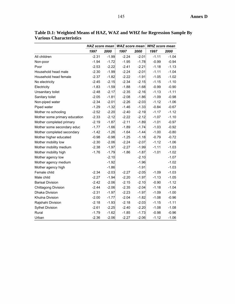
145 Annex D

Table D.1: Weighted Means of HAZ, WAZ and WHZ for Regression Sample By Various Characteristics

HAZ score mean WAZ score mean WHZ score mean 1997 2000 1997 2000 1997 2000 All children -2.31 -1.99 -2.24 -2.01 -1.11 -1.04 Non-poor -1.94 -1.72 -1.95 -1.78 -0.99 -0.94 Poor -2.53 -2.22 -2.41 -2.21 -1.18 -1.13 Household head male -2.30 -1.99 -2.24 -2.01 -1.11 -1.04 Household head female -2.37 -1.82 -2.22 -1.91 -1.05 -1.02 No electricity -2.45 -2.15 -2.34 -2.15 -1.15 -1.10 Electricity -1.83 -1.59 -1.88 -1.68 -0.99 -0.90 Unsanitary toilet -2.48 -2.17 -2.35 -2.16 -1.13 -1.11 Sanitary toilet -2.05 -1.81 -2.08 -1.86 -1.09 -0.98 Non-piped water -2.34 -2.01 -2.26 -2.03 -1.12 -1.06 Piped water -1.29 -1.32 -1.46 -1.33 -0.84 -0.67 Mother no schooling -2.52 -2.20 -2.40 -2.19 -1.17 -1.12 Mother some primary education -2.33 -2.12 -2.22 -2.12 -1.07 -1.10 Mother completed primary -2.19 -1.87 -2.11 -1.89 -1.01 -0.97 Mother some secondary educ -1.77 -1.66 -1.89 -1.74 -1.03 -0.92 Mother completed secondary -1.42 -1.26 -1.64 -1.44 -1.00 -0.80 Mother higher educated -0.98 -0.98 -1.25 -1.18 -0.79 -0.72 Mother mobility low -2.30 -2.06 -2.24 -2.07 -1.12 -1.06 Mother mobility medium -2.38 -1.97 -2.27 -1.99 -1.11 -1.03 Mother mobility high -1.76 -1.79 -1.86 -1.87 -1.01 -1.02 Mother agency low -2.10 -2.10 -1.07 Mother agency medium -1.92 -1.96 -1.02 Mother agency high -1.86 -1.91 -1.03 Female child -2.34 -2.03 -2.27 -2.05 -1.09 -1.03 Male child -2.27 -1.94 -2.20 -1.97 -1.13 -1.05 Barisal Division -2.42 -2.06 -2.15 -2.10 -0.90 -1.12 Chittagong Division -2.44 -2.06 -2.35 -2.04 -1.18 -1.04 Dhaka Division -2.31 -1.97 -2.23 -1.97 -1.09 -1.00 Khulna Division -2.00 -1.77 -2.04 -1.82 -1.08 -0.96 Rajshahi Division -2.18 -1.93 -2.18 -2.03 -1.15 -1.11 Sylhet Division -2.61 -2.25 -2.40 -2.20 -1.08 -1.08 Rural -1.79 -1.62 -1.85 -1.73 -0.98 -0.96 Urban -2.36 -2.06 -2.27 -2.06 -1.12 -1.06

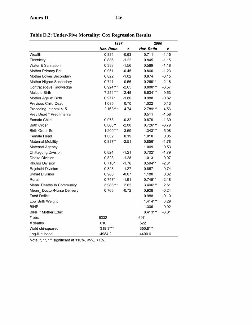
Annex D 146

Table D.2: Under-Five Mortality: Cox Regression Results 1997 2000 Haz. Ratio z Haz. Ratio z Wealth 0.834 -0.63 0.711 -1.15 Electricity 0.836 -1.22 0.845 -1.15 Water & Sanitation 0.383 -1.56 0.569 -1.18 Mother Primary Ed 0.951 -0.45 0.860 -1.23 Mother Lower Secondary 0.822 -1.02 0.974 -0.15 Mother Higher Secondary 0.741 -0.56 0.269** -2.18 Contraceptive Knowledge 0.924*** -2.65 0.880*** -3.57 Multiple Birth 7.254*** 12.45 6.534*** 9.53 Mother Age At Birth 0.977* -1.80 0.988 -0.82 Previous Child Dead 1.095 0.70 1.022 0.13 Preceding Interval <15 2.163*** 4.74 2.789*** 4.56 Prev Dead * Prec Interval 0.511 -1.58 Female Child 0.973 -0.32 0.879 -1.39 Birth Order 0.868** -2.00 0.726*** -3.79 Birth Order Sq 1.209*** 3.59 1.343*** 5.08 Female Head 1.032 0.19 1.010 0.05 Maternal Mobility 0.837** -2.51 0.856* -1.78 Maternal Agency 1.009 0.53 Chittagong Division 0.824 -1.21 0.702* -1.79 Dhaka Division 0.823 -1.28 1.013 0.07 Khulna Division 0.716* -1.76 0.594** -2.31 Rajshahi Division 0.823 -1.27 0.867 -0.74 Sylhet Division 0.988 -0.07 1.180 0.82 Rural 0.747* -1.91 0.745** -2.18 Mean_Deaths In Community 3.988*** 2.62 3.406*** 2.61 Mean_ Doctor/Nurse Delivery 0.768 -0.72 0.928 -0.24 Food Deficit 0.988 -0.10 Low Birth Weight 1.414*** 3.29 BINP 1.306 0.92 BINP * Mother Educ 0.413*** -3.01 # obs 6332 6974 # deaths 610 522 Wald chi-squared 319.3*** 350.8*** Log-likelihood -4984.2 -4400.6 Note: *, **, *** significant at <10%, <5%, <1%.

147 Annex D

Table D.3: Results of OLS and Two-Step Regressions of HAZ Score 1997 (OLS) 1997 (2-step) 2000 (OLS) 2000 (2-step) Coeff. t Coeff. t Coeff. t Coeff. t

Wealth 0.525*** 3.00 0.502* 2.86 0.481*** 3.28 0.401*** 2.73Finished Floor 0.057 0.59 0.058 0.60 -0.023 -0.29 -0.013 -0.17Electricity 0.228*** 3.25 0.214*** 3.05 0.164*** 2.98 0.145*** 2.62Sanitary Toilet 0.102** 1.96 0.100* 1.92 0.033 0.73 0.031 0.68Piped Water 0.165 1.16 0.141 0.98 0.031 0.32 -0.007 -0.07Mother Primary Educ 0.072 1.24 0.062 1.08 0.036 0.73 -0.003 -0.05Mother Lower Secondary 0.316*** 3.92 0.294*** 3.62 0.243*** 3.58 0.222*** 3.25Mother Higher Second 0.687*** 4.23 0.659*** 4.04 0.505*** 4.15 0.413*** 3.32Adult/Child Ratio 0.071*** 2.93 0.070*** 2.89 0.014 0.79 0.012 0.70Mother Age 0.023*** 3.59 0.021*** 3.20 0.025*** 4.42 0.023*** 4.10Female Head -0.043 -0.44 -0.038 -0.38 0.063 0.71 0.067 0.74Mother Mobility 0.019 0.53 0.008 0.21 0.035 1.03 0.008 0.23Mother Agency 0.014* 1.89 0.013* 1.83Log Mother Height 0.968*** 3.86 0.971*** 3.85 0.743*** 3.49 0.743*** 3.50Female Child -0.154** -2.32 -0.160** -2.42 -0.115* -1.86 -0.146** -2.39Female * Wealth 0.237 1.37 0.248 1.44 0.195 1.41 0.221 1.62Birth Order -0.113** -2.56 -0.120*** -2.75 -0.164*** -3.83 -0.198*** -4.54Birth Order Square 0.037 0.89 0.050 1.23 0.075* 1.87 0.110*** 2.66Prec Interval<24 -0.126** -2.37 -0.115** -2.16 -0.220*** -4.36 -0.192*** -3.76Child’s Age -0.071*** -10.89 -0.069*** -10.46 -0.045*** -7.95 -0.042*** -7.42Child’s Age Sq/10 0.083*** 8.39 0.081*** 8.15 0.051*** 6.04 0.048*** 5.66Rural 0.155* 1.74 0.139 1.55 -0.050 -0.72 -0.084 -1.18Born Feb-Mar*Rural -0.139* -1.86 -0.145* -1.95 -0.251*** -3.41 -0.253*** -3.47Born Apr-May*Rural -0.137* -1.71 -0.142* -1.77 -0.078 -1.07 -0.082 -1.14Born Jun-Jul*Rural -0.149* -1.83 -0.152* -1.87 -0.015 -0.20 -0.017 -0.23Born Aug-Sep*Rural -0.012 -0.16 -0.016 -0.21 0.040 0.54 0.035 0.49Born Oct-Nov*Rural 0.006 0.08 0.003 0.04 0.042 0.64 0.042 0.65Chittagong Division -0.026 -0.31 -0.041 -0.49 -0.052 -0.67 -0.091 -1.15Dhaka Division 0.144* 1.86 0.126 1.62 0.044 0.57 0.056 0.72Khulna Division 0.437*** 4.93 0.408*** 4.54 0.190** 2.41 0.134* 1.67Rajshahi Division 0.370*** 4.69 0.350*** 4.41 0.196** 2.48 0.177** 2.23Sylhet Division -0.130 -1.40 -0.117 -1.26 -0.087 -1.00 -0.024 -0.27Mean_Measles Vacc. 0.046 0.15 0.050 0.16 0.139 0.62 0.144 0.63Food Deficit -0.073 -1.57 -0.077* -1.66Low Birth Weight -0.424*** -8.23 -0.358*** -6.78BINP 0.241* 1.92 0.266** 2.09BINP*Educ -0.183*** -2.91 -0.231*** -3.56Constant -6.753*** -5.27 -6.613*** -5.13 -5.448*** -4.97 -5.121*** -4.67Lambda 0.815** 2.00 1.993*** 3.70# obs 4258 4258 4719 4719 F-statistic 24.7*** 24.1*** 21.0*** 21.2*** R-squared 0.159 0.160 0.153 0.158 Note: *, **, *** significant at <10%, <5%, <1%.

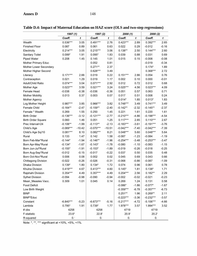
Annex D 148

Table D.4: Impact of Maternal Education on HAZ score (OLS and two-step regressions) 1997 (1) 1997 (2) 2000 (1) 2000 (2) Coeff. t Coeff. t Coeff. t Coeff. t Wealth 0.536*** 3.05 0.491*** 2.76 0.423*** 2.89 0.392*** 2.65Finished Floor 0.087 0.89 0.061 0.63 0.022 0.29 -0.012 -0.16Electricity 0.214*** 3.05 0.215*** 3.06 0.138** 2.50 0.144*** 2.60Sanitary Toilet 0.099* 1.91 0.095* 1.83 0.039 0.88 0.031 0.69Piped Water 0.208 1.45 0.145 1.01 0.015 0.15 -0.008 -0.08Mother Primary Educ 0.052 0.81 -0.019 -0.34Mother Lower Secondary 0.271** 2.37 0.174* 1.89Mother Higher Second 0.628*** 3.49 0.368*** 2.72Literacy 0.171*** 2.66 0.019 0.22 0.151*** 2.86 0.054 0.76Contraception 0.021 1.29 0.019 1.17 0.002 0.10 0.000 -0.01Adult/Child Ratio 0.074*** 3.04 0.071*** 2.92 0.012 0.72 0.012 0.68Mother Age 0.023*** 3.59 0.021*** 3.24 0.025*** 4.56 0.023*** 4.09Female Head -0.038 -0.38 -0.036 -0.36 0.051 0.57 0.063 0.71Mother Mobility 0.013 0.37 0.003 0.07 0.017 0.51 0.008 0.24Mother Agency 0.014* 1.85 0.013* 1.83Log Mother Height 0.987*** 3.85 0.966*** 3.82 0.748*** 3.49 0.741*** 3.49Female Child -0.164** -2.47 -0.159** -2.40 -0.142** -2.32 -0.145** -2.37Female * Wealth 0.269 1.55 0.250 1.45 0.221 1.61 0.220 1.61Birth Order -0.136*** -3.12 -0.121*** -2.77 -0.210*** -4.86 -0.198*** -4.54Birth Order Square 0.060 1.46 0.051 1.25 0.117*** 2.85 0.110*** 2.67Prec Interval<24 -0.106** -1.99 -0.113** -2.13 -0.183*** -3.61 -0.191*** -3.76Child’s Age -0.069*** -10.42 -0.070*** -10.51 -0.042*** -7.40 -0.042*** -7.39Child’s Age Sq/10 0.081*** 8.10 0.082*** 8.21 0.048*** 5.60 0.048*** 5.64Rural 0.133 1.47 0.142 1.58 -0.087 -1.23 -0.084 -1.19Born Feb-Mar*Rural -0.144* -1.94 -0.146** -1.96 -0.254*** -3.48 -0.253*** -3.47Born Apr-May*Rural -0.134* -1.67 -0.143* -1.78 -0.080 -1.10 -0.083 -1.15Born Jun-Jul*Rural -0.155* -1.91 -0.153* -1.89 -0.019 -0.26 -0.018 -0.25Born Aug-Sep*Rural -0.012 -0.15 -0.017 -0.22 0.037 0.50 0.035 0.48Born Oct-Nov*Rural 0.006 0.08 0.002 0.02 0.045 0.69 0.043 0.66Chittagong Division -0.022 -0.26 -0.026 -0.31 -0.068 -0.86 -0.087 -1.09Dhaka Division 0.139* 1.80 0.134* 1.72 0.074 0.96 0.061 0.78Khulna Division 0.419*** 4.67 0.413*** 4.60 0.145* 1.81 0.138* 1.71Rajshahi Division 0.354*** 4.49 0.357*** 4.49 0.204*** 2.56 0.182** 2.29Sylhet Division -0.094 -0.98 -0.090 -0.94 -0.002 -0.02 -0.021 -0.23Mean_Measles Vacc. 0.309 1.01 0.045 0.14 0.269 1.24 0.131 0.58Food Deficit -0.086* -1.86 -0.077* -1.67Low Birth Weight -0.359*** -6.78 -0.357*** -6.73BINP 0.251** 1.96 0.269** 2.11BINP*Educ -0.223*** -3.36 -0.232*** -3.57Constant -6.840*** -5.23 -6.673*** -5.16 -5.217*** -4.72 -5.106*** -4.66Lambda 0.795* 1.91 0.739* 1.77 1.978*** 3.57 1.994*** 3.52# obs 4258 4258 4719 4719 F-statistic 23.6* 22.8* 20.9* 20.2*R-squared 0.1 0.1 0.1 0.1

Note: *, **, *** significant at <10%, <5%, <1%.

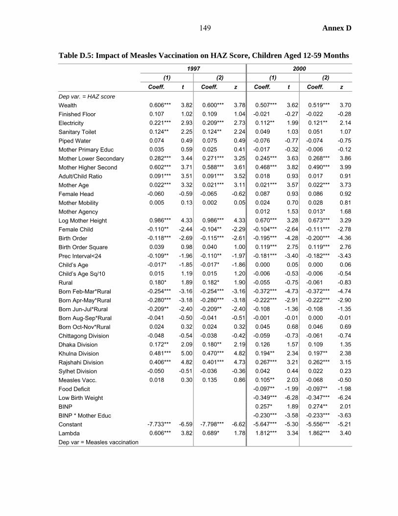
149 Annex D

Table D.5: Impact of Measles Vaccination on HAZ Score, Children Aged 12-59 Months

1997 2000 (1) (2) (1) (2) Coeff. t Coeff. z Coeff. t Coeff. z

Dep var. = HAZ score Wealth 0.606*** 3.82 0.600*** 3.78 0.507*** 3.62 0.519*** 3.70Finished Floor 0.107 1.02 0.109 1.04 -0.021 -0.27 -0.022 -0.28Electricity 0.221*** 2.93 0.209*** 2.73 0.112** 1.99 0.121** 2.14Sanitary Toilet 0.124** 2.25 0.124** 2.24 0.049 1.03 0.051 1.07Piped Water 0.074 0.49 0.075 0.49 -0.076 -0.77 -0.074 -0.75Mother Primary Educ 0.035 0.59 0.025 0.41 -0.017 -0.32 -0.006 -0.12Mother Lower Secondary 0.282*** 3.44 0.271*** 3.25 0.245*** 3.63 0.268*** 3.86Mother Higher Second 0.602*** 3.71 0.588*** 3.61 0.468*** 3.82 0.490*** 3.99Adult/Child Ratio 0.091*** 3.51 0.091*** 3.52 0.018 0.93 0.017 0.91Mother Age 0.022*** 3.32 0.021*** 3.11 0.021*** 3.57 0.022*** 3.73Female Head -0.060 -0.59 -0.065 -0.62 0.087 0.93 0.086 0.92Mother Mobility 0.005 0.13 0.002 0.05 0.024 0.70 0.028 0.81Mother Agency 0.012 1.53 0.013* 1.68Log Mother Height 0.986*** 4.33 0.986*** 4.33 0.670*** 3.28 0.673*** 3.29Female Child -0.110** -2.44 -0.104** -2.29 -0.104*** -2.64 -0.111*** -2.78Birth Order -0.118*** -2.69 -0.115*** -2.61 -0.195*** -4.28 -0.200*** -4.36Birth Order Square 0.039 0.98 0.040 1.00 0.119*** 2.75 0.119*** 2.76Prec Interval<24 -0.109** -1.96 -0.110** -1.97 -0.181*** -3.40 -0.182*** -3.43Child’s Age -0.017* -1.85 -0.017* -1.86 0.000 0.05 0.000 0.06Child’s Age Sq/10 0.015 1.19 0.015 1.20 -0.006 -0.53 -0.006 -0.54Rural 0.180* 1.89 0.182* 1.90 -0.055 -0.75 -0.061 -0.83Born Feb-Mar*Rural -0.254*** -3.16 -0.254*** -3.16 -0.372*** -4.73 -0.372*** -4.74Born Apr-May*Rural -0.280*** -3.18 -0.280*** -3.18 -0.222*** -2.91 -0.222*** -2.90Born Jun-Jul*Rural -0.209** -2.40 -0.209** -2.40 -0.108 -1.36 -0.108 -1.35Born Aug-Sep*Rural -0.041 -0.50 -0.041 -0.51 -0.001 -0.01 0.000 -0.01Born Oct-Nov*Rural 0.024 0.32 0.024 0.32 0.045 0.68 0.046 0.69Chittagong Division -0.048 -0.54 -0.038 -0.42 -0.059 -0.73 -0.061 -0.74Dhaka Division 0.172** 2.09 0.180** 2.19 0.126 1.57 0.109 1.35Khulna Division 0.481*** 5.00 0.470*** 4.82 0.194** 2.34 0.197** 2.38Rajshahi Division 0.406*** 4.82 0.401*** 4.73 0.267*** 3.21 0.262*** 3.15Sylhet Division -0.050 -0.51 -0.036 -0.36 0.042 0.44 0.022 0.23Measles Vacc. 0.018 0.30 0.135 0.86 0.105** 2.03 -0.068 -0.50Food Deficit -0.097** -1.99 -0.097** -1.98Low Birth Weight -0.349*** -6.28 -0.347*** -6.24BINP 0.257* 1.89 0.274** 2.01BINP * Mother Educ -0.230*** -3.58 -0.233*** -3.63Constant -7.733*** -6.59 -7.798*** -6.62 -5.647*** -5.30 -5.556*** -5.21Lambda 0.606*** 3.82 0.689* 1.78 1.812*** 3.34 1.862*** 3.40Dep var = Measles vaccination

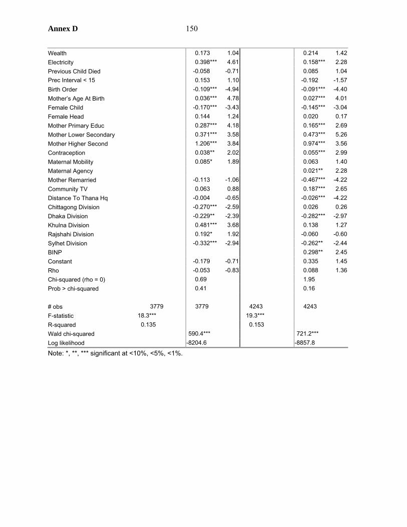
Annex D 150

Wealth 0.173 1.04 0.214 1.42Electricity 0.398*** 4.61 0.158*** 2.28Previous Child Died -0.058 -0.71 0.085 1.04Prec Interval < 15 0.153 1.10 -0.192 -1.57Birth Order -0.109*** -4.94 -0.091*** -4.40Mother’s Age At Birth 0.036*** 4.78 0.027*** 4.01Female Child -0.170*** -3.43 -0.145*** -3.04Female Head 0.144 1.24 0.020 0.17Mother Primary Educ 0.287*** 4.18 0.165*** 2.69Mother Lower Secondary 0.371*** 3.58 0.473*** 5.26Mother Higher Second 1.206*** 3.84 0.974*** 3.56Contraception 0.038** 2.02 0.055*** 2.99Maternal Mobility 0.085* 1.89 0.063 1.40Maternal Agency 0.021** 2.28Mother Remarried -0.113 -1.06 -0.467*** -4.22Community TV 0.063 0.88 0.187*** 2.65Distance To Thana Hq -0.004 -0.65 -0.026*** -4.22Chittagong Division -0.270*** -2.59 0.026 0.26Dhaka Division -0.229** -2.39 -0.282*** -2.97Khulna Division 0.481*** 3.68 0.138 1.27Rajshahi Division 0.192* 1.92 -0.060 -0.60Sylhet Division -0.332*** -2.94 -0.262** -2.44BINP 0.298** 2.45Constant -0.179 -0.71 0.335 1.45Rho -0.053 -0.83 0.088 1.36Chi-squared (rho = 0) 0.69 1.95 Prob > chi-squared 0.41 0.16 # obs 3779 3779 4243 4243 F-statistic 18.3*** 19.3*** R-squared 0.135 0.153 Wald chi-squared 590.4*** 721.2*** Log likelihood -8204.6 -8857.8

Note: *, **, *** significant at <10%, <5%, <1%.

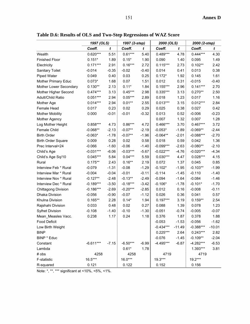
151 Annex D

Table D.6: Results of OLS and Two-Step Regressions of WAZ Score 1997 (OLS) 1997 (2-step) 2000 (OLS) 2000 (2-step) Coeff. t Coeff. t Coeff. t Coeff. t

Wealth 0.620*** 5.51 0.61*** 5.40 0.489*** 4.78 0.444*** 4.30Finished Floor 0.151* 1.89 0.15* 1.90 0.090 1.40 0.095 1.49Electricity 0.171*** 2.91 0.16*** 2.72 0.115*** 2.73 0.102** 2.42Sanitary Toilet -0.014 -0.35 -0.02 -0.40 0.014 0.41 0.013 0.38Piped Water 0.049 0.40 0.03 0.25 0.172* 1.92 0.145 1.61Mother Primary Educ 0.073* 1.68 0.07 1.51 0.012 0.31 -0.015 -0.40Mother Lower Secondary 0.130** 2.13 0.11* 1.84 0.155*** 2.96 0.141*** 2.70Mother Higher Second 0.474*** 3.13 0.45*** 2.98 0.335*** 3.13 0.270** 2.50Adult/Child Ratio 0.051*** 2.94 0.05*** 2.89 0.018 1.23 0.017 1.16Mother Age 0.014*** 2.94 0.01** 2.55 0.013*** 3.15 0.012*** 2.84Female Head 0.017 0.23 0.02 0.29 0.025 0.38 0.027 0.42Mother Mobility 0.000 -0.01 -0.01 -0.32 0.013 0.52 -0.006 -0.23Mother Agency 0.007 1.32 0.007 1.28Log Mother Height 0.858*** 4.73 0.86*** 4.72 0.466*** 3.70 0.467*** 3.72Female Child -0.068** -2.13 -0.07** -2.19 -0.053* -1.89 -0.069** -2.44Birth Order -0.063* -1.78 -0.07** -1.96 -0.064** -2.01 -0.088*** -2.70Birth Order Square 0.009 0.28 0.02 0.58 0.018 0.59 0.042 1.36Prec Interval<24 -0.066 -1.60 -0.06 -1.40 -0.099*** -2.63 -0.080** -2.10Child’s Age -0.031*** -6.06 -0.03*** -5.67 -0.022*** -4.76 -0.020*** -4.34Child’s Age Sq/10 0.045*** 5.84 0.04*** 5.59 0.030*** 4.47 0.028*** 4.15Rural 0.175** 2.43 0.16** 2.19 0.072 1.37 0.045 0.85Interview Feb * Rural -0.079 -1.31 -0.08 -1.29 -0.102* -1.95 -0.103** -1.99Interview Mar * Rural -0.004 -0.04 -0.01 -0.11 -0.114 -1.45 -0.110 -1.40Interview Nov * Rural -0.127** -2.48 -0.13** -2.49 -0.094 -1.64 -0.084 -1.46Interview Dec * Rural -0.189*** -3.50 -0.18*** -3.42 -0.106* -1.78 -0.101* -1.70Chittagong Division -0.186*** -2.69 -0.20*** -2.85 0.012 0.16 -0.008 -0.11Dhaka Division -0.056 -0.90 -0.07 -1.12 0.026 0.36 0.041 0.57Khulna Division 0.165** 2.28 0.14* 1.94 0.197*** 3.19 0.159** 2.54Rajshahi Division 0.033 0.48 0.02 0.27 0.088 1.39 0.078 1.23Sylhet Division -0.108 -1.40 -0.10 -1.30 -0.051 -0.74 -0.005 -0.07Mean_Measles Vacc. 0.238 1.17 0.24 1.18 0.376 1.87 0.378 1.88Food Deficit -0.053 -1.53 -0.056 -1.62Low Birth Weight -0.434*** -11.49 -0.388*** -10.01BINP 0.225*** 2.64 0.243*** 2.82BINP * Educ -0.076 -1.45 -0.109** -2.04Constant -6.611*** -7.15 -6.50*** -6.99 -4.495*** -6.87 -4.282*** -6.53Lambda 0.61* 1.78 1.393*** 3.81# obs 4258 4258 4719 4719F-statistic 16.5*** 16.0*** 19.3*** 19.2*** R-squared 0.121 0.122 0.152 0.156 Note: *, **, *** significant at <10%, <5%, <1%.

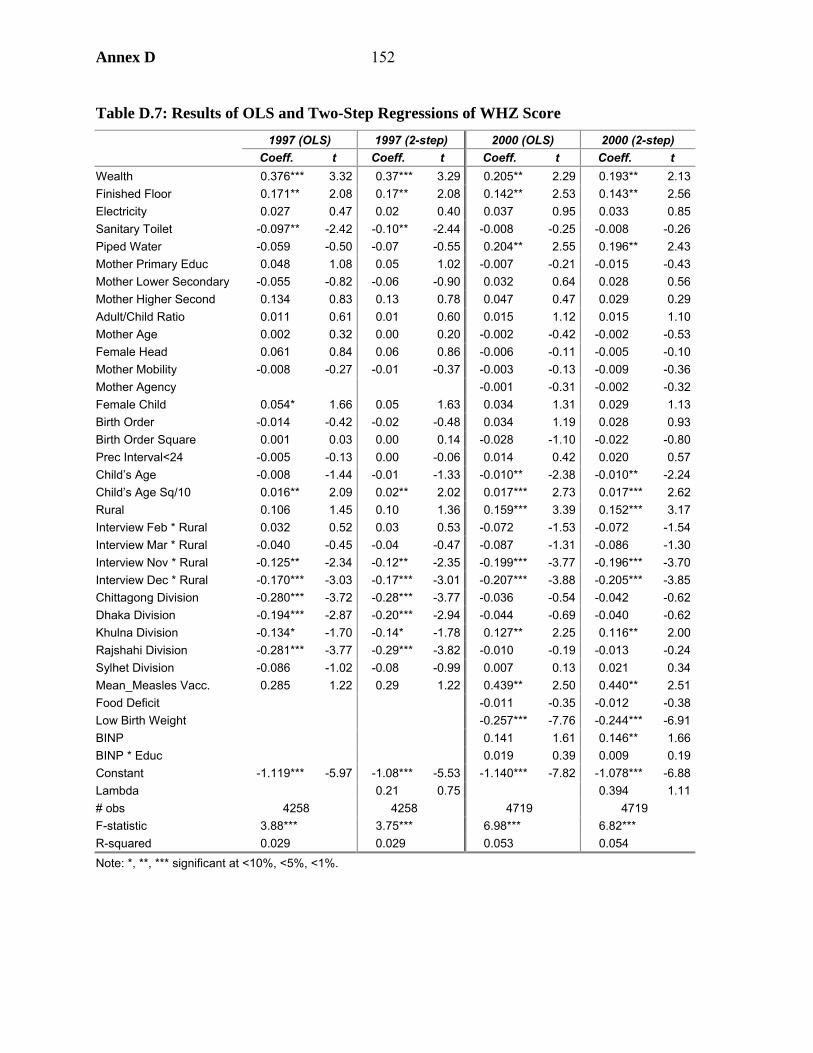
Annex D 152

Table D.7: Results of OLS and Two-Step Regressions of WHZ Score 1997 (OLS) 1997 (2-step) 2000 (OLS) 2000 (2-step) Coeff. t Coeff. t Coeff. t Coeff. t

Wealth 0.376*** 3.32 0.37*** 3.29 0.205** 2.29 0.193** 2.13Finished Floor 0.171** 2.08 0.17** 2.08 0.142** 2.53 0.143** 2.56Electricity 0.027 0.47 0.02 0.40 0.037 0.95 0.033 0.85Sanitary Toilet -0.097** -2.42 -0.10** -2.44 -0.008 -0.25 -0.008 -0.26Piped Water -0.059 -0.50 -0.07 -0.55 0.204** 2.55 0.196** 2.43Mother Primary Educ 0.048 1.08 0.05 1.02 -0.007 -0.21 -0.015 -0.43Mother Lower Secondary -0.055 -0.82 -0.06 -0.90 0.032 0.64 0.028 0.56Mother Higher Second 0.134 0.83 0.13 0.78 0.047 0.47 0.029 0.29Adult/Child Ratio 0.011 0.61 0.01 0.60 0.015 1.12 0.015 1.10Mother Age 0.002 0.32 0.00 0.20 -0.002 -0.42 -0.002 -0.53Female Head 0.061 0.84 0.06 0.86 -0.006 -0.11 -0.005 -0.10Mother Mobility -0.008 -0.27 -0.01 -0.37 -0.003 -0.13 -0.009 -0.36Mother Agency -0.001 -0.31 -0.002 -0.32Female Child 0.054* 1.66 0.05 1.63 0.034 1.31 0.029 1.13Birth Order -0.014 -0.42 -0.02 -0.48 0.034 1.19 0.028 0.93Birth Order Square 0.001 0.03 0.00 0.14 -0.028 -1.10 -0.022 -0.80Prec Interval<24 -0.005 -0.13 0.00 -0.06 0.014 0.42 0.020 0.57Child’s Age -0.008 -1.44 -0.01 -1.33 -0.010** -2.38 -0.010** -2.24Child’s Age Sq/10 0.016** 2.09 0.02** 2.02 0.017*** 2.73 0.017*** 2.62Rural 0.106 1.45 0.10 1.36 0.159*** 3.39 0.152*** 3.17Interview Feb * Rural 0.032 0.52 0.03 0.53 -0.072 -1.53 -0.072 -1.54Interview Mar * Rural -0.040 -0.45 -0.04 -0.47 -0.087 -1.31 -0.086 -1.30Interview Nov * Rural -0.125** -2.34 -0.12** -2.35 -0.199*** -3.77 -0.196*** -3.70Interview Dec * Rural -0.170*** -3.03 -0.17*** -3.01 -0.207*** -3.88 -0.205*** -3.85Chittagong Division -0.280*** -3.72 -0.28*** -3.77 -0.036 -0.54 -0.042 -0.62Dhaka Division -0.194*** -2.87 -0.20*** -2.94 -0.044 -0.69 -0.040 -0.62Khulna Division -0.134* -1.70 -0.14* -1.78 0.127** 2.25 0.116** 2.00Rajshahi Division -0.281*** -3.77 -0.29*** -3.82 -0.010 -0.19 -0.013 -0.24Sylhet Division -0.086 -1.02 -0.08 -0.99 0.007 0.13 0.021 0.34Mean_Measles Vacc. 0.285 1.22 0.29 1.22 0.439** 2.50 0.440** 2.51Food Deficit -0.011 -0.35 -0.012 -0.38Low Birth Weight -0.257*** -7.76 -0.244*** -6.91BINP 0.141 1.61 0.146** 1.66BINP * Educ 0.019 0.39 0.009 0.19Constant -1.119*** -5.97 -1.08*** -5.53 -1.140*** -7.82 -1.078*** -6.88Lambda 0.21 0.75 0.394 1.11# obs 4258 4258 4719 4719 F-statistic 3.88*** 3.75*** 6.98*** 6.82*** R-squared 0.029 0.029 0.053 0.054 Note: *, **, *** significant at <10%, <5%, <1%.

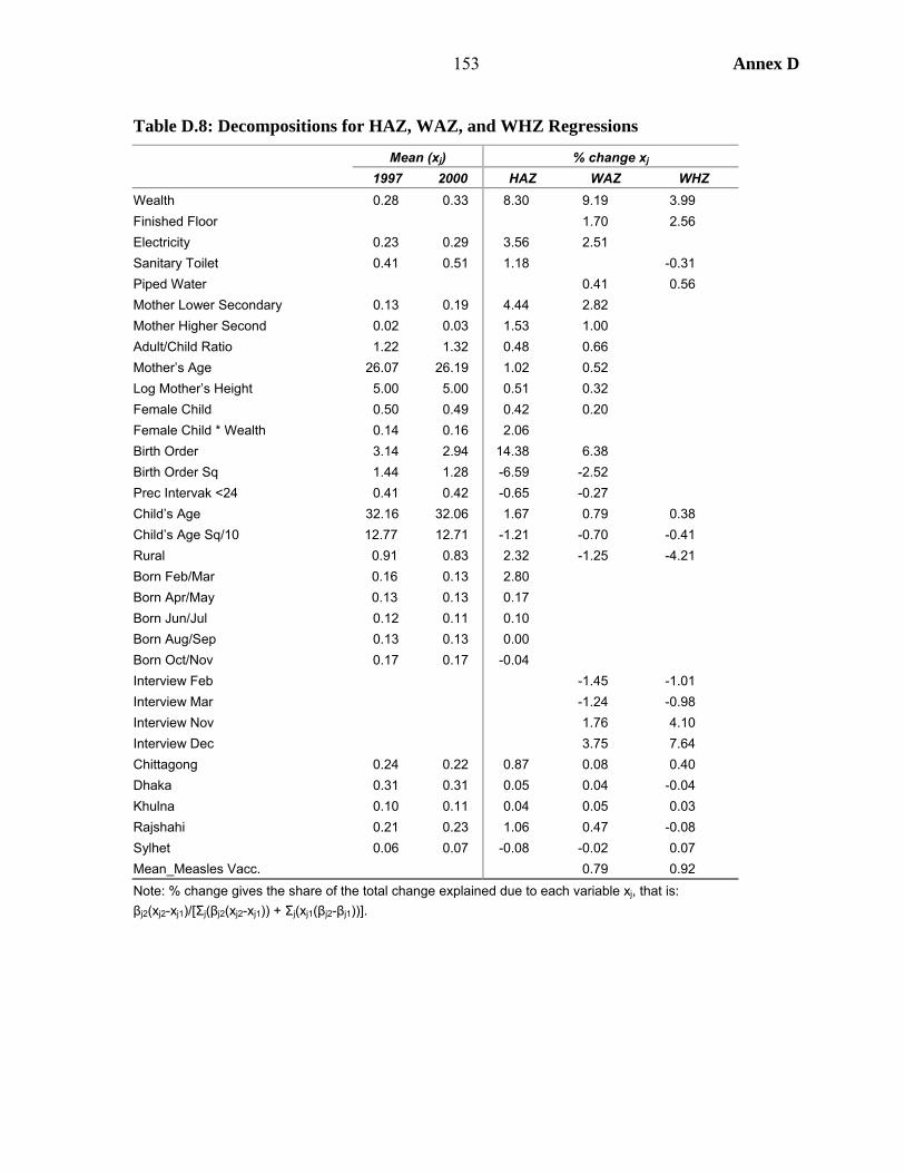
153 Annex D

Table D.8: Decompositions for HAZ, WAZ, and WHZ Regressions

Mean (xj) % change xj 1997 2000 HAZ WAZ WHZ

Wealth 0.28 0.33 8.30 9.19 3.99 Finished Floor 1.70 2.56 Electricity 0.23 0.29 3.56 2.51 Sanitary Toilet 0.41 0.51 1.18 -0.31 Piped Water 0.41 0.56 Mother Lower Secondary 0.13 0.19 4.44 2.82 Mother Higher Second 0.02 0.03 1.53 1.00 Adult/Child Ratio 1.22 1.32 0.48 0.66 Mother’s Age 26.07 26.19 1.02 0.52 Log Mother’s Height 5.00 5.00 0.51 0.32 Female Child 0.50 0.49 0.42 0.20 Female Child * Wealth 0.14 0.16 2.06 Birth Order 3.14 2.94 14.38 6.38 Birth Order Sq 1.44 1.28 -6.59 -2.52 Prec Intervak <24 0.41 0.42 -0.65 -0.27 Child’s Age 32.16 32.06 1.67 0.79 0.38 Child’s Age Sq/10 12.77 12.71 -1.21 -0.70 -0.41 Rural 0.91 0.83 2.32 -1.25 -4.21 Born Feb/Mar 0.16 0.13 2.80 Born Apr/May 0.13 0.13 0.17 Born Jun/Jul 0.12 0.11 0.10 Born Aug/Sep 0.13 0.13 0.00 Born Oct/Nov 0.17 0.17 -0.04 Interview Feb -1.45 -1.01 Interview Mar -1.24 -0.98 Interview Nov 1.76 4.10 Interview Dec 3.75 7.64 Chittagong 0.24 0.22 0.87 0.08 0.40 Dhaka 0.31 0.31 0.05 0.04 -0.04 Khulna 0.10 0.11 0.04 0.05 0.03 Rajshahi 0.21 0.23 1.06 0.47 -0.08 Sylhet 0.06 0.07 -0.08 -0.02 0.07 Mean_Measles Vacc. 0.79 0.92 Note: % change gives the share of the total change explained due to each variable xj, that is: βj2(xj2-xj1)/[Σj(βj2(xj2-xj1)) + Σj(xj1(βj2-βj1))].

Annex E 154

Annex E. Women’s Agency, Household Structure, and Health Outcomes

1. Bangladesh is often characterized as a country in which women face many restrictions. This is certainly so: recent data from DHS show that not many more than one in five women are solely responsible for decisions relating to their own health, and the large majority are not permitted to travel outside their household unaccompanied. But it is also easy to overstate the case, and to ignore that things are changing, changing quite rapidly.

2. This paper begins by presenting data from the three DHS surveys from Bangladesh on women’s role in decisionmaking (women’s agency) and women’s mobility. These issues are linked to household structure, which is shown here to be a critical determinant of female autonomy. Other determinants that may lay behind the changes with have taken place in the 1990s, such as increased women’s work outside the home and the spread of secondary education, are also analyzed.

3. A related issue is age at marriage. The data show that the age at marriage is increasing. In most countries, raising age at marriage has been a critical factor in reducing fertility. However, it is argued that this is not likely to be the case in Bangladesh.

Household Structure

4. Household surveys contain a household roster in which basic information on all household members is collected. In DHS, as in most other surveys, all people who spend the night before the survey are included in the roster, with a further question asking if that person is a “usual resident” of the household. The roster also includes people deemed to be household members but absent the previous night. Not collecting this information means that female-headed households are “over-identified,” that is, a household in which the adult male is absent for prolonged reasons for work is not recorded in the roster, so that the wife may appear as the household head.

5. The first question asked about each person in the roster is their relationship to the household head. The responses to this question are tabulated in Table E.1, for all 54,627 respondents of the DHS 1999/2000 survey and, in the second column, excluding the 3,190 respondents who were not usual residents. The final two columns tabulate the share for usual residents by sex.

6. The “core” of each household is the head, their husband or wife and children. Just under half of household members are children, around one-third of men are household heads and one-third of women the wife of the head. As explored below, extended households are not uncommon, as shown by 4.0 percent who are parents or parents-in-law and the 2.5 percent who are a son or daughter-in-law. The gender disaggregation shows these to be daughters-in-law: it is uncommon for a man to live with his parents-in-law (only 0.4 percent of men are the son-in-law of the head compared to the 5 percent of women who are daughters-in-law). Comparing the shares for the whole roster for those of “usual residents” show that grandchildren, siblings,

155 Annex E

and other relatives are the most likely visitors. The small percentage of “not related” are mostly not visitors, so these people are most likely live-in servants. The category co-spouse received zero responses. This does not mean there are no polygamous households, since the relationship shown is that to the household head; rather, it means there are no polygamous households in which one of the wives was identified as the head. For just eight people in total their relationship was not known or not stated.

7. The data in the household roster can be used to identify five household types, where this classification is fully exhaustive and mutually exclusive (i.e., it covers all households with no overlaps):1

• Extended: a household including either a parent, parent-in-law, or son or daughter-in-law of the household head. White (1992) distinguishes between extended and joint households, where the latter live in the same compound but separate production and consumption (crucially do not eat together, which is the definition of household adopted in some household surveys). It is not possible with DHS data to distinguish these two household types,2 and White anyhow notes that the distinction is often more nominal than real.

• Nuclear: a household including the spouse of the head, but no parent, parent-in-law, or son or daughter-in-law

• Female-headed household: we do not simply take those households for which a woman is listed as the head, as some of these women have husbands or live with another adult male (Table E.1). Rather, we classify as FHH those cases where a woman is identified as the head and there is no spouse, male parent, or son-in-law listed in the roster.

• Single-male-headed household: where there is no spouse listed. • Polygamous: where the head has more than one wife.

8. The last column of Table E.2 shows the breakdown of the 9,853 households covered by DHS 1999/2000 into these five categories. The majority of households are nuclear, though just over one-third are extended. The share of female-headed households is likely overstated for the 1. The following calculations were made including only “usual residents” from the household roster. Those people identified as not related to the household head were not included since, as mentioned above, these people are most likely live-in servants.

2. As discussed below, DHS 1999/2000 contains data on if a woman makes the decision on what to cook each day by herself. Where this is the case for more than one woman, then this fact may indicate a joint household.

Table E.1: Relationship to Household Head (percent)

Usual residents only Whole roster Total Male Female Head 18.0 19.1 34.7 3.3 Wife or husband 15.8 16.7 0.2 33.5 Son/daughter 43.9 45.3 50.6 40.0 Son/daughter-in-law 2.8 2.7 0.4 5.0 Grandchild 5.0 4.1 4.3 3.9 Parent 3.5 3.6 1.3 6.0 Parent-in-law 0.5 0.3 0.1 0.6 Brother/sister 3.4 3.1 3.9 2.4 Co-spouse 0.0 0.0 0.0 0.0 Other relative 5.3 3.2 2.9 3.6 Adopted/foster child 0.3 0.3 0.3 0.2 Not related 1.5 1.5 1.4 1.6 Don’t know/missing 0.0 0.0 0.0 0.0 Absolute number 54,627 51,437 25,877 25,560

Source: DHS 1999/2000

Annex E 156

reasons given above: that is, many of these households will have an absent male (husband) who supports the family and visits occasionally. A woman left alone after death or desertion of the spouse is more likely to return to her parents’ household.3 The share of female-headed households can also be overstated where co-spouses live in separate households, which would also explain why the share of polygamous households is low at less than one percent. Unsurprising is that the share of single-male-headed households is low, since men typically remarry on death of, or separation from, the spouse (White 1992; Kabeer 2004).

9. Also unsurprising is the correlation between household size and structure: the majority of households between two to six people are nuclear, but larger households are more likely to be extended (Figure E.1). The largest household in the dataset is an extended family of 25 people consisting of an 80-year-old man and his 60-year-old wife, their four sons with their wives, one unmarried son aged 30, and 14 grandchildren.4

10. There is also a relationship between household structure and economic well-being as measured by an asset index based on housing quality and ownership of consumer durables (see Annex C.3 on the construction of the asset index); see Table E.2. Extended families are more common among higher income groups, with the converse being true for nuclear families. Given that there is also the link between household size and structure this finding means that large (extended) households are better off: a fact that runs counter to “standard economics poverty profiles” in which household size is correlated with poverty, but is of no surprise to anthropologists who report that households with resources need and attract labor, mostly through the family.5 For example, White (1992) attributes the likelihood of a household disintegrating to its lack of resources.

Table E.2: Household Types by Income Group

Income group Low Middle High Total

Extended 24.6 37.1 41.3 33.5 Nuclear 64.8 54.6 50.9 57.5 Female head 8.8 6.6 6.4 7.4 Single male headed 1.0 0.8 0.5 0.8 Polygamous 0.8 0.9 0.9 0.8 Absolute no. of households 3,639 3,865 2,350 9,854

Source: DHS 1999/2000

3. For example, there are 70 women in the dataset aged over 35 and living with a parent, half of these were formerly married – and the other half are currently married, there are no never-married women in this group (there are only 19 never-married women from the 6,209 aged over 35 in the whole dataset).

4. The age of the oldest son is given as 50. The ages of the adults – reported as 30, 35, 40, 45, 50, 60, and 80 – clearly suffer from what is called “heaping,” i.e., rounding by respondents to the nearest 5 or 10. Nonetheless, it seems likely that the oldest son at least is the product of a previous marriage.

5. See White (2001) for more discussion of this contradiction in findings.

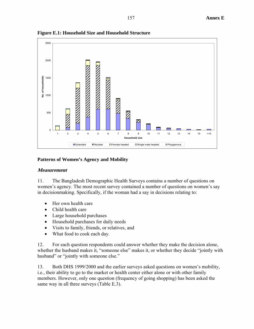
157 Annex E

Figure E.1: Household Size and Household Structure

0

500

1000

1500

2000

2500

1 2 3 4 5 6 7 8 9 10 11 12 13 14 15 >15

Household size

No.

of h

ouse

hold

s

Extended Nuclear Female headed Single male headed Polygamous

Patterns of Women’s Agency and Mobility

Measurement

11. The Bangladesh Demographic Health Surveys contains a number of questions on women’s agency. The most recent survey contained a number of questions on women’s say in decisionmaking. Specifically, if the woman had a say in decisions relating to:

• Her own health care • Child health care • Large household purchases • Household purchases for daily needs • Visits to family, friends, or relatives, and • What food to cook each day.

12. For each question respondents could answer whether they make the decision alone, whether the husband makes it, “someone else” makes it, or whether they decide “jointly with husband” or “jointly with someone else.”

13. Both DHS 1999/2000 and the earlier surveys asked questions on women’s mobility, i.e., their ability to go to the market or health center either alone or with other family members. However, only one question (frequency of going shopping) has been asked the same way in all three surveys (Table E.3).

Annex E 158

14. For questions on frequency of going shopping or going outside village/ town/city respondents could answer “never,” “several times a year,” “once a month or more.” Answers were ranked/ordered accordingly. For questions on whether they go or can go outside village, town, or city or to health center respondents could choose to answer one of the following: “don’t go,” “alone,” “with husband,” “with children,” or “other.” For our purposes going “with husband” and “other” were pooled and the responses ranked/ordered with don’t go as lowest ranking, followed by going “with others” (including husband), with children, and finally alone.

Women’s Agency: Descriptive Analysis

15. Table E.4 summarizes the six aspects of women’s agency collected by DHS 1999/2000. These data are tabulated for three groups: all respondents (which are ever-married women aged 11-49), currently married women in male-headed households (since we argue below that women in female-headed households largely make decisions by default), and women who live with their mother-in-law, since the literature suggests that these women will have less say in decisionmaking. The data indeed shows that women living with their mother-in-law have a diminished role in decisionmaking compared with other women, whereas “someone else” (presumably the mother-in-law) is much more likely to have a say – and implicitly that women in female-headed households decide more than those in male-headed ones. We return to this issue below.

16. Other than the decision about what to cook, less than one in five women are solely responsible for the decisions shown, but over half are involved in the decision either solely or jointly. Women are least commonly solely responsible for the decision regarding large purchases; but husbands are also less commonly solely responsible for this decision, which is the most common joint decision.

17. Women’s involvement in decisionmaking on matters related to their own health and that of their children is low. Forty-three percent of women have no say in the decisions on their own health, rising to 52 percent for women living with their mother-in-law. With respect to decisions related to child health, these figures are 34 and 42 percent, respectively.

Table E.3: Questions on Women’s Mobility Contained in Different DHS Questionnaires

DHS93 DHS96 DHS99 If do go outside village/town/city alone X X If can go outside village/town/city alone X X X If go to health center/hospital alone X X If can go health center/hospital alone X X X Frequency of going shopping X X X With whom do they go shopping X X Frequency of going outside village/town/city X* X X * In 1993 the question was whether they go to another part of their village/town/city rather than if they leave it.

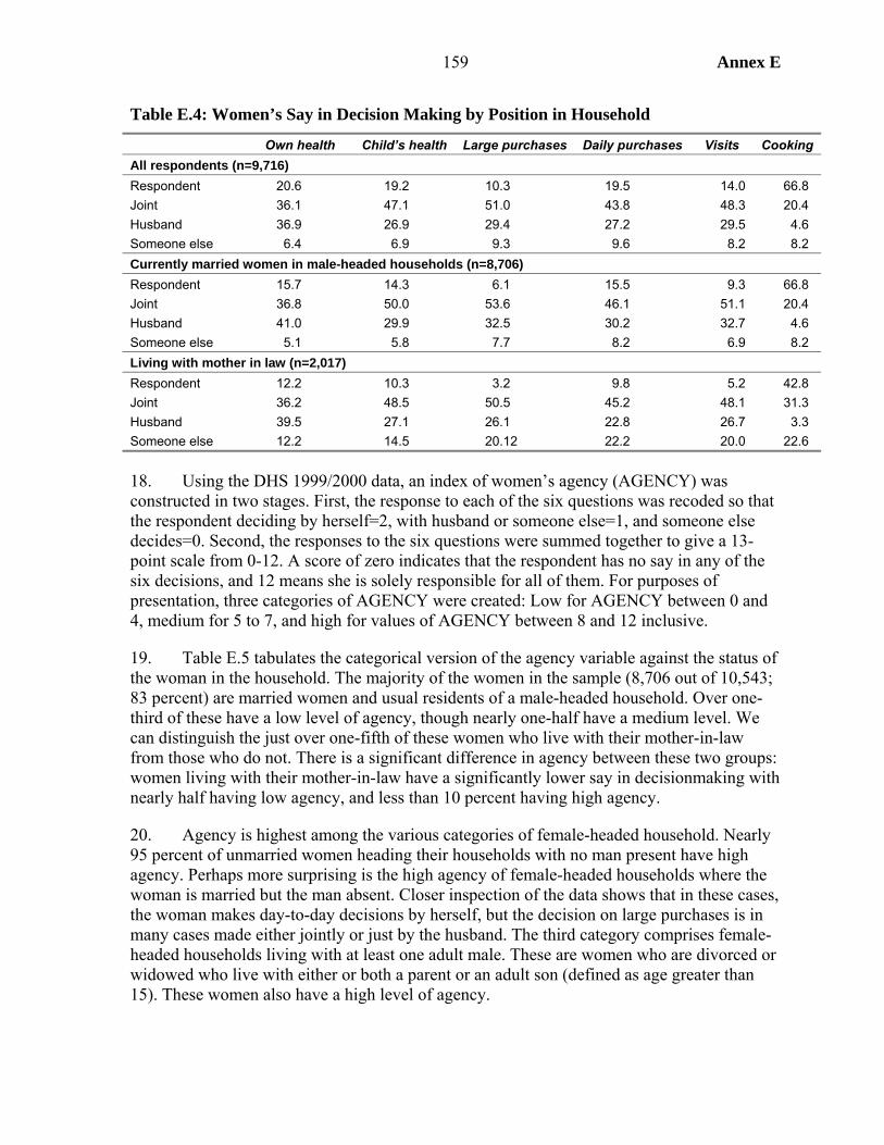
159 Annex E

Table E.4: Women’s Say in Decision Making by Position in Household

Own health Child’s health Large purchases Daily purchases Visits Cooking All respondents (n=9,716) Respondent 20.6 19.2 10.3 19.5 14.0 66.8 Joint 36.1 47.1 51.0 43.8 48.3 20.4 Husband 36.9 26.9 29.4 27.2 29.5 4.6 Someone else 6.4 6.9 9.3 9.6 8.2 8.2 Currently married women in male-headed households (n=8,706) Respondent 15.7 14.3 6.1 15.5 9.3 66.8 Joint 36.8 50.0 53.6 46.1 51.1 20.4 Husband 41.0 29.9 32.5 30.2 32.7 4.6 Someone else 5.1 5.8 7.7 8.2 6.9 8.2 Living with mother in law (n=2,017) Respondent 12.2 10.3 3.2 9.8 5.2 42.8 Joint 36.2 48.5 50.5 45.2 48.1 31.3 Husband 39.5 27.1 26.1 22.8 26.7 3.3 Someone else 12.2 14.5 20.12 22.2 20.0 22.6 18. Using the DHS 1999/2000 data, an index of women’s agency (AGENCY) was constructed in two stages. First, the response to each of the six questions was recoded so that the respondent deciding by herself=2, with husband or someone else=1, and someone else decides=0. Second, the responses to the six questions were summed together to give a 13-point scale from 0-12. A score of zero indicates that the respondent has no say in any of the six decisions, and 12 means she is solely responsible for all of them. For purposes of presentation, three categories of AGENCY were created: Low for AGENCY between 0 and 4, medium for 5 to 7, and high for values of AGENCY between 8 and 12 inclusive.

19. Table E.5 tabulates the categorical version of the agency variable against the status of the woman in the household. The majority of the women in the sample (8,706 out of 10,543; 83 percent) are married women and usual residents of a male-headed household. Over one-third of these have a low level of agency, though nearly one-half have a medium level. We can distinguish the just over one-fifth of these women who live with their mother-in-law from those who do not. There is a significant difference in agency between these two groups: women living with their mother-in-law have a significantly lower say in decisionmaking with nearly half having low agency, and less than 10 percent having high agency.

20. Agency is highest among the various categories of female-headed household. Nearly 95 percent of unmarried women heading their households with no man present have high agency. Perhaps more surprising is the high agency of female-headed households where the woman is married but the man absent. Closer inspection of the data shows that in these cases, the woman makes day-to-day decisions by herself, but the decision on large purchases is in many cases made either jointly or just by the husband. The third category comprises female-headed households living with at least one adult male. These are women who are divorced or widowed who live with either or both a parent or an adult son (defined as age greater than 15). These women also have a high level of agency.

Annex E 160

Table E.5: Women’s Agency by Status Within the Household

Women’s agency Woman’s marital status Household type Low Medium High No. of obs.

Male-headed households 37.9 48.1 14.0 8,706 o/w Living with mother-in-law 49.2 43.4 7.5 2,015 Other 34.5 49.5 16.0 6,691

Married

Female-headed (husband not present) 3.1 12.9 84.0 136 FHH with no adult male 2.7 3.3 94.0 162 FHH with adult male 3.3 16.9 79.9 112 Unmarried Other 35.7 31.3 33.0 574

Total 36.9 45.0 18.2 10,543 21. An implication of this analysis is that when looking at the correlates of agency it makes sense to focus on married women in male-headed households, who are anyway the bulk of the sample. Including women in female-headed households would undermine the power of the results, since these women are the decisionmakers by virtue of their status and regardless of their other characteristics (wealth, religion, etc.).

22. Bivariate tabulations are shown for the former group of women against various characteristics in Table E.6. The relationship between the variables shown is statistically significant in all cases. The main area where there is no difference is the similar distribution of agency between Muslim and Hindu women, although the small group of women from other religions do have higher agency. A women’s agency increases with household wealth, her age, whether she has had a child or not (with a son counting for more than a daughter), and if she is working (with working for cash having more of an impact). A slight kink in the pattern is the lopsided U-shaped relationship between high agency and asset quintile, with women in the lowest quintile having slightly greater agency than those in the second and third. This result may reflect that poorer households are more likely to be nuclear, and women have higher agency in these households. Multivariate analysis is used below to separate out these effects.

Women’s Mobility: Descriptive Analysis

23. An analysis of women’s mobility using the same methodology as above reveals that mobility and agency related to the same factors, despite the fact that, as shown below, the two are only imperfectly correlated.

24. Women’s mobility is most restricted when it comes to going shopping, indicating that purdah and social norms continue to render the marketplace off limits to women. Thus, a whole 68 percent of all women and three-fourths of women who live with their mother-in-law never go shopping. In comparison, only 4 to 5 percent of women cannot leave their village, town, or city of residence or go to the health center.

25. As is the case for intra-household agency, women who live with their mother-in-law have less mobility than other women. Fewer of these women can leave their village, town, or city alone and more can only go if accompanied by their husband or someone else. The pattern is the same for going to the health center and going shopping.

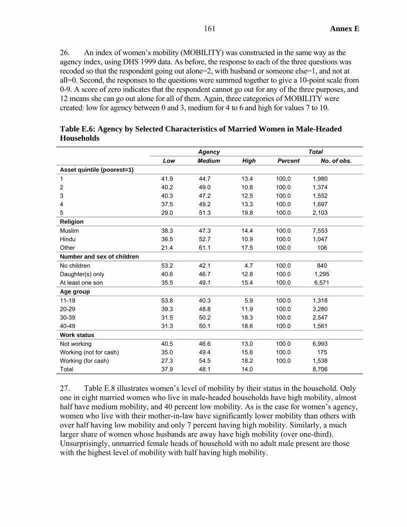
161 Annex E

26. An index of women’s mobility (MOBILITY) was constructed in the same way as the agency index, using DHS 1999 data. As before, the response to each of the three questions was recoded so that the respondent going out alone=2, with husband or someone else=1, and not at all=0. Second, the responses to the questions were summed together to give a 10-point scale from 0-9. A score of zero indicates that the respondent cannot go out for any of the three purposes, and 12 means she can go out alone for all of them. Again, three categories of MOBILITY were created: low for agency between 0 and 3, medium for 4 to 6 and high for values 7 to 10.

Table E.6: Agency by Selected Characteristics of Married Women in Male-Headed Households

Agency Total Low Medium High Percent No. of obs. Asset quintile (poorest=1) 1 41.9 44.7 13.4 100.0 1,980 2 40.2 49.0 10.8 100.0 1,374 3 40.3 47.2 12.5 100.0 1,552 4 37.5 49.2 13.3 100.0 1,697 5 29.0 51.3 19.8 100.0 2,103 Religion Muslim 38.3 47.3 14.4 100.0 7,553 Hindu 36.5 52.7 10.9 100.0 1,047 Other 21.4 61.1 17.5 100.0 106 Number and sex of children No children 53.2 42.1 4.7 100.0 840 Daughter(s) only 40.6 46.7 12.8 100.0 1,295 At least one son 35.5 49.1 15.4 100.0 6,571 Age group 11-19 53.8 40.3 5.9 100.0 1,318 20-29 39.3 48.8 11.9 100.0 3,280 30-39 31.5 50.2 18.3 100.0 2,547 40-49 31.3 50.1 18.6 100.0 1,561 Work status Not working 40.5 46.6 13.0 100.0 6,993 Working (not for cash) 35.0 49.4 15.6 100.0 175 Working (for cash) 27.3 54.5 18.2 100.0 1,538 Total 37.9 48.1 14.0 8,706

27. Table E.8 illustrates women’s level of mobility by their status in the household. Only one in eight married women who live in male-headed households have high mobility, almost half have medium mobility, and 40 percent low mobility. As is the case for women’s agency, women who live with their mother-in-law have significantly lower mobility than others with over half having low mobility and only 7 percent having high mobility. Similarly, a much larger share of women whose husbands are away have high mobility (over one-third). Unsurprisingly, unmarried female heads of household with no adult male present are those with the highest level of mobility with half having high mobility.

Annex E 162

28. Analyzing women’s mobility by selected characteristics for married women in male-headed households (Table E.9) reveals a pattern similar to that of women’s agency. There is a U-shaped relationship between assets and mobility with women in wealth quintiles 1 and 2 having greater mobility than the women in quintile 3 and women in the poorest quintile also having greater mobility than women in quintile 4. Such a relationship is consistent with the notion that the poorest women in Bangladesh often are those who adhere least to purdah because their financial situation forces them to venture outside to work: the largest percentage of women who undertake paid work belong to the poorest asset quintile,6 while, as illustrated in Table E.8, a larger proportion of women who work have high mobility. This is consistent with the notion that women from better-off households can better afford to adhere to purdah and hence restrict mobility to a greater extent.

Table E.7: Women’s Mobility

Can leave

village/town Can go to

health center Go

shopping All respondents (n=9,716) Alone 17.0 30.0 13.8 With children 49.5 24.2 6.4 With husband or someone else 29.2 40.6 11.7 Cannot go 4.3 5.2 68.1 Currently married women in male-headed households (n=8,704) Alone 14.8 28.4 11.5 With children 50.1 23.4 6.1 With husband or someone else 30.7 43.0 12.2 Cannot go 4.3 5.2 70.2 Living with mother in law (n=2,017) Alone 10.2 22.6 6.6 With children 38.3 16.4 3.9 With husband or someone else 46.2 54.3 15.2 Cannot go 5.3 6.7 74.4

Table E.8: Women’s Mobility by Status Within the Household Women’s mobility

Woman’s marital status Household type Low Medium High No. of obs. Male-headed households 41.5 46.2 12.3 8,706 o/w Living with mother-in-law 55.1 37.4 7.6 2,015 Other 37.4 48.8 13.7 6,691

Married

Female-headed (husband not present) 14.0 54.7 31.3 136 FHH with no adult male 8.7 40.7 50.5 162 FHH with adult male 5.7 55.3 39.1 112 Unmarried Other 26.0 45.0 29.0 574

Total 40.0 45.7 14.3 10,543

6. There is a strict monotonic inverse relationship between asset quintile and the proportion of women in either paid or unpaid work. Twenty-five percent of women in the poorest quintile engage in paid work, and 4.6 in unpaid. For the top quintile these figures are 14.8 and 0.9 percent, respectively.

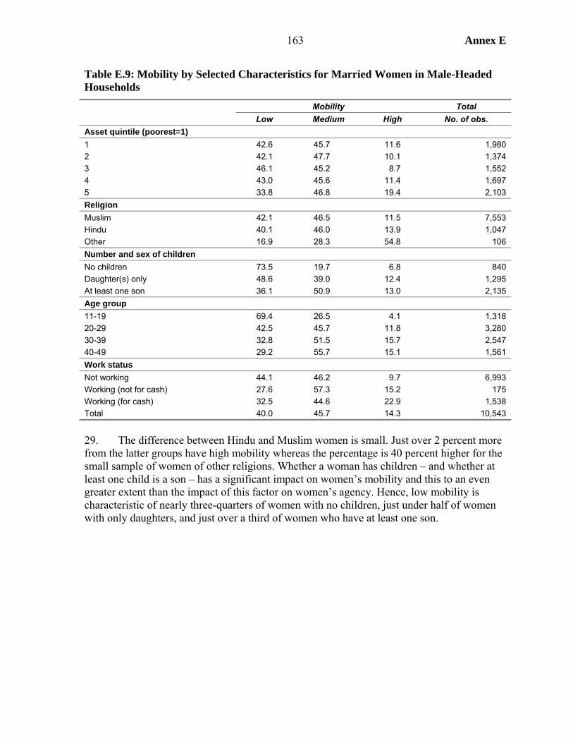
163 Annex E

Table E.9: Mobility by Selected Characteristics for Married Women in Male-Headed Households

Mobility Total Low Medium High No. of obs. Asset quintile (poorest=1) 1 42.6 45.7 11.6 1,980 2 42.1 47.7 10.1 1,374 3 46.1 45.2 8.7 1,552 4 43.0 45.6 11.4 1,697 5 33.8 46.8 19.4 2,103 Religion Muslim 42.1 46.5 11.5 7,553 Hindu 40.1 46.0 13.9 1,047 Other 16.9 28.3 54.8 106 Number and sex of children No children 73.5 19.7 6.8 840 Daughter(s) only 48.6 39.0 12.4 1,295 At least one son 36.1 50.9 13.0 2,135 Age group 11-19 69.4 26.5 4.1 1,318 20-29 42.5 45.7 11.8 3,280 30-39 32.8 51.5 15.7 2,547 40-49 29.2 55.7 15.1 1,561 Work status Not working 44.1 46.2 9.7 6,993 Working (not for cash) 27.6 57.3 15.2 175 Working (for cash) 32.5 44.6 22.9 1,538 Total 40.0 45.7 14.3 10,543

29. The difference between Hindu and Muslim women is small. Just over 2 percent more from the latter groups have high mobility whereas the percentage is 40 percent higher for the small sample of women of other religions. Whether a woman has children – and whether at least one child is a son – has a significant impact on women’s mobility and this to an even greater extent than the impact of this factor on women’s agency. Hence, low mobility is characteristic of nearly three-quarters of women with no children, just under half of women with only daughters, and just over a third of women who have at least one son.

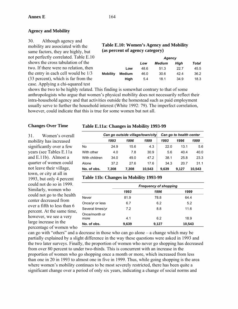
Annex E 164

Agency and Mobility

30. Although agency and mobility are associated with the same factors, they are highly, but not perfectly correlated. Table E.10 shows the cross tabulation of the two. If there were no relation, then the entry in each cell would be 1/3 (33 percent), which is far from the case. Applying a chi-squared test shows the two to be highly related. This finding is somewhat contrary to that of some anthropologists who argue that women’s physical mobility does not necessarily reflect their intra-household agency and that activities outside the homestead such as paid employment usually serve to further the household interest (White 1992: 79). The imperfect correlation, however, could indicate that this is true for some women but not all.

Changes Over Time

31. Women’s overall mobility has increased significantly over a few years (see Tables E.11a and E.11b). Almost a quarter of women could not leave their village, town, or city at all in 1993, but only 4 percent could not do so in 1999. Similarly, women who could not go to the health center decreased from over a fifth to less than 6 percent. At the same time, however, we see a very large increase in the percentage of women who can go with “others” and a decrease in those who can go alone – a change which may be partially explained by a slight difference in the way these questions were asked in 1993 and the two later surveys. Finally, the proportion of women who never go shopping has decreased from over 80 percent to under two-thirds. This is concurrent with an increase in the proportion of women who go shopping once a month or more, which increased from less than one in 20 in 1993 to almost one in five in 1999. Thus, while going shopping is the area where women’s mobility continues to be most severely restricted, there has been quite a significant change over a period of only six years, indicating a change of social norms and

Table E.10: Women’s Agency and Mobility (as percent of agency category) Agency Low Medium High Total

Low 48.6 51.3 22.7 45.5 Medium 46.0 30.6 42.4 36.2 Mobility

High 5.4 18.1 34.9 18.3

Table E.11a: Changes in Mobility 1993-99

Can go outside village/town/city Can go to health center 1993 1996 1999 1993 1996 1999 No 24.9 15.6 4.3 22.0 13.1 5.6With other 4.0 7.8 30.9 5.6 40.4 40.0With children 34.0 49.0 47.2 38.1 25.8 23.3Alone 37.2 27.6 17.6 34.3 20.7 31.1No. of obs. 7,308 7,308 10,543 9,639 9,127 10,543

Table 11b: Changes in Mobility 1993-99

Frequency of shopping 1993 1996 1999 Never 81.9 78.8 64.4 Once/yr or less 6.7 6.2 5.2 Several times/yr 7.2 8.8 11.6 Once/month or more 4.1 6.2 18.9 No. of obs. 9,639 9,127 10,543

165 Annex E

the practice of purdah. This does not mean that purdah is disappearing, but, as suggested by Kabeer (2002), it is adapting to changing socioeconomic conditions.

Multivariate Analysis

32. Regression analysis was performed for the agency and mobility indices and the health decision variables. The indices are discrete variables in the range 0-12 and 0-9, so might appear to be able to be treated as continuous variables using ordinary least squares. However, a tabulation shows both series to be right censored (observations are bunched at the upper limit) so that a tobit model is appropriate. The recoded agency and mobility variables related to health can be used as dependent variables in an ordered probit model. The sample in all cases is married women in male-headed households.

33. By and large, the results support the patterns shown in bivariate tabulations. The following results are particularly striking:

• Both age and age squared are significant, indicating that both agency and mobility increase with age, but then decrease after a certain threshold.7 The coefficients show this threshold to be in the early forties (see Table A.3). This variable may also pick up a “time effect” where older households afford women less agency and mobility. Having a child also increases agency, with the effect being stronger if the child is male.

• Both agency and mobility increase with educational status (the reference category is no education), though the effect of primary is not always significant. Given that there is a strong correlation between education and the level of the asset index (Table A.2), the fact that both sets of variables are frequently significant is striking, showing that the impact of education can operate independently of that through wealth.

• The three media variables, especially TV, have a strong effect, though reading a paper is not always significant.8

• Daughters-in-law have a strongly significantly lower level of agency and mobility. Mobility is higher for mothers-in-law but not agency.

• The inverted U with respect to wealth is evident for agency but not mobility. • Working has a strong positive effect, as does being a member of a credit organization. • Regional effects are high, with women in Sylhet and Barisal faring worst.9 Rural

women also have lower mobility and agency. • The small number of women from other religions (the reference category is Muslim)

have more agency and mobility. The Hindu dummy is negative but not significant.

In summary, the policy implications are that:

7. The age variables are more significant than one measuring the age gap between husband and wife, which is only significant when age is not included.

8. Analysis of other data shows that respondents saying they can read the paper often prove to have poor literacy, which will undermine the power of this variable.

9. Dummies were initially included for all regions with Dhaka as the reference region. Those with insignificant coefficients were dropped in the results reported here.

Annex E 166

• It is true that women often don’t have a say – so health and nutrition messages need to reach a wider audience.

• But agency and mobility can change over time, and are doing so in Bangladesh quite rapidly. Policy relevant factors that can affect this rate of change are communications (IEC), and education.

Age at Marriage in Bangladesh

34. The age at marriage is a well-known determinant of maternal and child health outcomes. Children born to young mothers are more likely to die, so that raising the age of marriage, especially in a country like Bangladesh in which births outside of marriage are extremely rare, will reduce infant mortality. Traditionally, rising age at marriage has been a driver of fertility reduction, though there are reasons to think that this effect may be muted in Bangladesh where age at marriage is indeed low, but fertility has already been substantially reduced (Annex F). Data from the Demographic Health Survey show surprisingly large changes in the age at marriage over a very short period. This paper analyses the determinants of age at marriage, and thus identifies factors behind these changes.

Marriage in Bangladesh

35. Virtually all women in Bangladesh get married. Data on over 110,000 women aged over 10 from the three DHS surveys shows that 99.4 percent of women aged over 30 have been married at some point (i.e., are currently or formerly married). Figure E.2(a) shows the marital status for women in different age groups.10 This graph shows that, over 30, only a tiny proportion of women have never been married. It also shows that the vast majority of women are married by their early 20s, and that virtually all are once they reach 25. As might be expected, older women are more likely to be formerly married since their husbands predecease them. Husbands dying before their wives is not only a result of the shorter life expectancy of males, but also the common large age differential in Bangladesh. Figure E.2(b) shows that men marry later than women, with the majority marrying by the time they are 30, rather than by their early 20s as is the case for women. Most men under 20 are not married, whereas most women are.

36. However, the age of marriage is changing. Despite the short period covered by the DHS surveys, which might be expected to be too short to pick up significant social trends, women in Bangladesh are getting married later. As shown in Table 1, the proportion of women married before they are 22 fell from 86 percent in the 1993 survey to 80 percent in 1999. The change is not among the youngest group – just under 5 percent of 10-15 year olds are married in all three surveys, but among those aged 16-21.

10. The data in this figure are from DHS 93 and DHS 99. The question required to construct the graph was not asked in DHS 96.

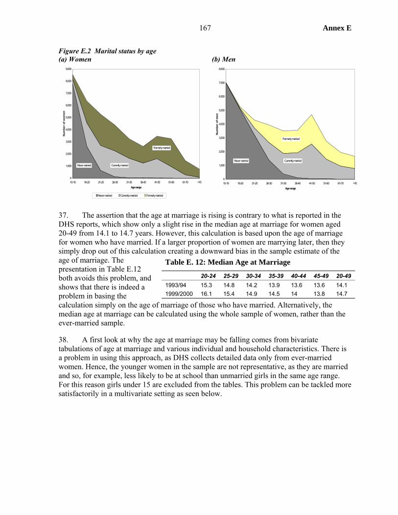
167 Annex E

Figure E.2 Marital status by age (a) Women (b) Men

0

1,000

2,000

3,000

4,000

5,000

6,000

7,000

8,000

9,000

10-15 16-20 21-25 26-30 31-35 36-40 41-50 51-60 61-70 >70

Age range

Num

ber o

f wom

en

Never married Currently married Formerly married

Never married Currently married

Formerly married

0

1,000

2,000

3,000

4,000

5,000

6,000

7,000

8,000

10-15 16-20 21-25 26-30 31-35 36-40 41-50 51-60 61-70 >70

Age range

Num

ber o

f men

Never married Currently married

Formerly married

37. The assertion that the age at marriage is rising is contrary to what is reported in the DHS reports, which show only a slight rise in the median age at marriage for women aged 20-49 from 14.1 to 14.7 years. However, this calculation is based upon the age of marriage for women who have married. If a larger proportion of women are marrying later, then they simply drop out of this calculation creating a downward bias in the sample estimate of the age of marriage. The presentation in Table E.12 both avoids this problem, and shows that there is indeed a problem in basing the calculation simply on the age of marriage of those who have married. Alternatively, the median age at marriage can be calculated using the whole sample of women, rather than the ever-married sample.

38. A first look at why the age at marriage may be falling comes from bivariate tabulations of age at marriage and various individual and household characteristics. There is a problem in using this approach, as DHS collects detailed data only from ever-married women. Hence, the younger women in the sample are not representative, as they are married and so, for example, less likely to be at school than unmarried girls in the same age range. For this reason girls under 15 are excluded from the tables. This problem can be tackled more satisfactorily in a multivariate setting as seen below.

Table E. 12: Median Age at Marriage

20-24 25-29 30-34 35-39 40-44 45-49 20-49 1993/94 15.3 14.8 14.2 13.9 13.6 13.6 14.1 1999/2000 16.1 15.4 14.9 14.5 14 13.8 14.7

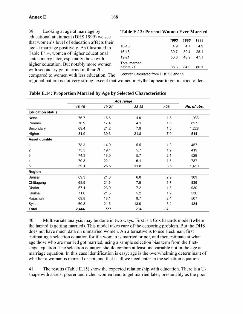
Annex E 168

39. Looking at age at marriage by educational attainment (DHS 1999) we see that women’s level of education affects their age at marriage positively. As illustrated in Table E/14, women of higher educational status marry later, especially those with higher education. But notably more women with secondary get married in their 20s compared to women with less education. The regional pattern is not very strong, except that women in Sylhet appear to get married older.

Table E.14: Proportion Married by Age by Selected Characteristics Age range

16-18 19-21 22-25 >26 No. of obs. Education status None 76.7 16.6 4.9 1.8 1,033 Primary 76.9 17.4 4.1 1.6 827 Secondary 69.4 21.2 7.9 1.5 1,228 Higher 31.9 39.3 21.8 7.0 514 Asset quintile 1 78.3 14.9 5.5 1.3 457 2 73.3 19.1 5.7 1.9 419 3 74.3 18.0 5.7 2.1 529 4 70.3 22.1 6.1 1.5 787 5 59.1 25.5 11.8 3.5 1,410 Region Barisal 69.3 21.0 6.8 2.9 309 Chittagong 68.9 21.5 7.9 1.7 836 Dhaka 67.1 23.9 7.2 1.8 930 Khulna 71.6 21.3 5.2 1.9 536 Rajashahi 69.8 18.1 9.7 2.4 507 Sylhet 60.3 21.5 13.0 5.2 484 Total 2,444 777 294 87

40. Multivariate analysis may be done in two ways. First is a Cox hazards model (where the hazard is getting married). This model takes care of the censoring problem. But the DHS does not have much data on unmarried women. An alternative is to use Heckman, first estimating a selection equation for if a woman is married or not, and then estimate at what age those who are married got married, using a sample selection bias term from the first-stage equation. The selection equation should contain at least one variable not in the age at marriage equation. In this case identification is easy: age is the overwhelming determinant of whether a woman is married or not, and that is all we need enter in the selection equation.

41. The results (Table E.15) show the expected relationship with education. There is a U-shape with assets: poorer and richer women tend to get married later, presumably as the poor

Table E.13: Percent Women Ever Married

1993 1996 1999 10-15 4.9 4.7 4.9 16-18 30.7 30.4 28.1 19-21 50.6 48.9 47.1 Total married before 21 86.3 84.0 80.1

Source: Calculated from DHS 93 and 99

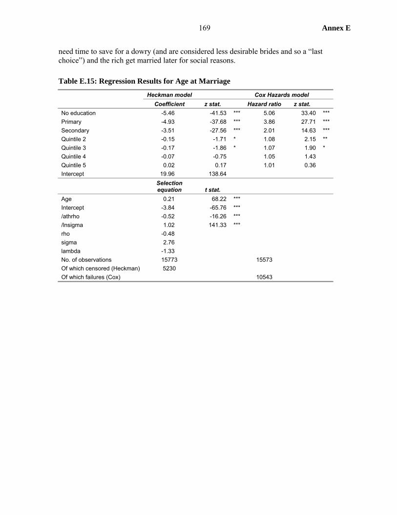
169 Annex E

need time to save for a dowry (and are considered less desirable brides and so a “last choice”) and the rich get married later for social reasons.

Table E.15: Regression Results for Age at Marriage

Heckman model Cox Hazards model Coefficient z stat. Hazard ratio z stat.

No education -5.46 -41.53 *** 5.06 33.40 *** Primary -4.93 -37.68 *** 3.86 27.71 *** Secondary -3.51 -27.56 *** 2.01 14.63 *** Quintile 2 -0.15 -1.71 * 1.08 2.15 ** Quintile 3 -0.17 -1.86 * 1.07 1.90 * Quintile 4 -0.07 -0.75 1.05 1.43 Quintile 5 0.02 0.17 1.01 0.36 Intercept 19.96 138.64

Selection equation t stat.

Age 0.21 68.22 *** Intercept -3.84 -65.76 *** /athrho -0.52 -16.26 *** /lnsigma 1.02 141.33 *** rho -0.48 sigma 2.76 lambda -1.33 No. of observations 15773 15573 Of which censored (Heckman) 5230 Of which failures (Cox) 10543

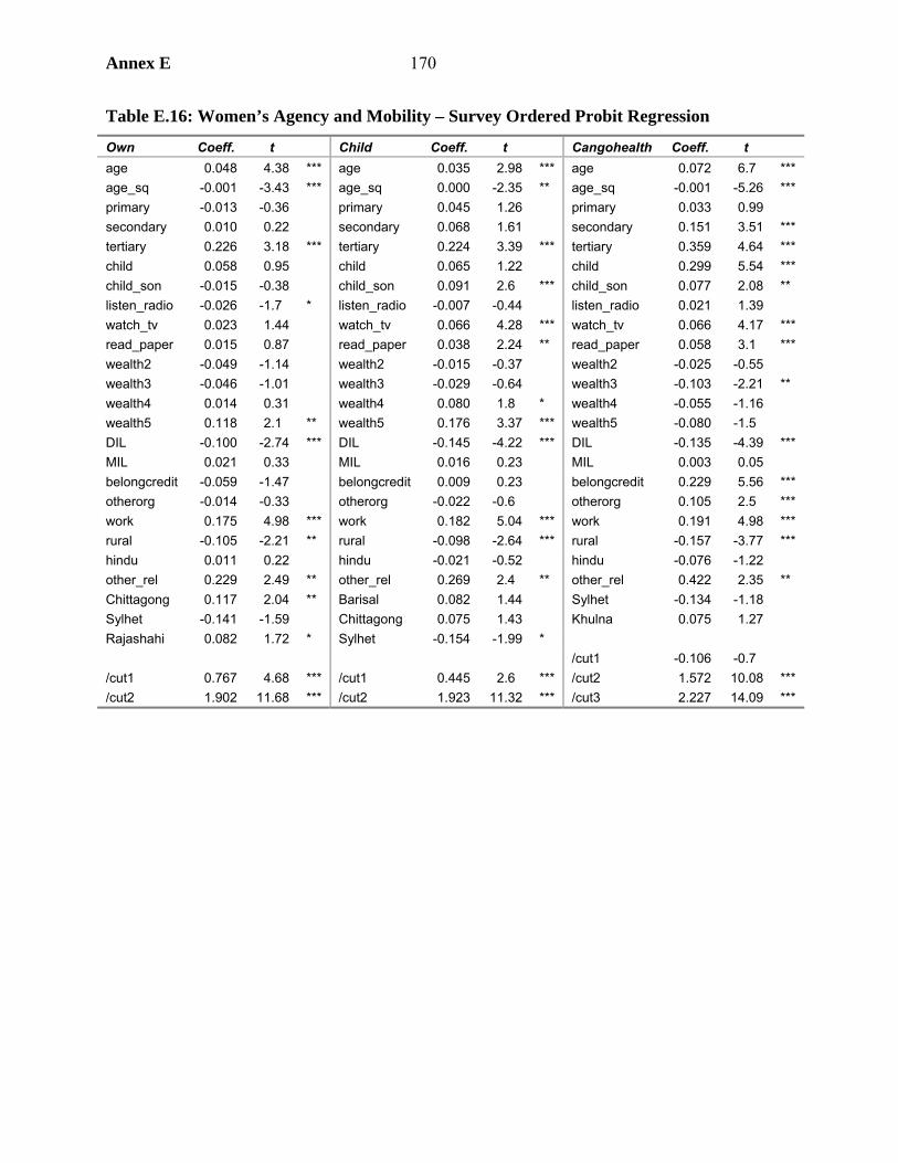
Annex E 170

Table E.16: Women’s Agency and Mobility – Survey Ordered Probit Regression

Own Coeff. t Child Coeff. t Cangohealth Coeff. t age 0.048 4.38 *** age 0.035 2.98 *** age 0.072 6.7 *** age_sq -0.001 -3.43 *** age_sq 0.000 -2.35 ** age_sq -0.001 -5.26 *** primary -0.013 -0.36 primary 0.045 1.26 primary 0.033 0.99 secondary 0.010 0.22 secondary 0.068 1.61 secondary 0.151 3.51 *** tertiary 0.226 3.18 *** tertiary 0.224 3.39 *** tertiary 0.359 4.64 *** child 0.058 0.95 child 0.065 1.22 child 0.299 5.54 *** child_son -0.015 -0.38 child_son 0.091 2.6 *** child_son 0.077 2.08 ** listen_radio -0.026 -1.7 * listen_radio -0.007 -0.44 listen_radio 0.021 1.39 watch_tv 0.023 1.44 watch_tv 0.066 4.28 *** watch_tv 0.066 4.17 *** read_paper 0.015 0.87 read_paper 0.038 2.24 ** read_paper 0.058 3.1 *** wealth2 -0.049 -1.14 wealth2 -0.015 -0.37 wealth2 -0.025 -0.55 wealth3 -0.046 -1.01 wealth3 -0.029 -0.64 wealth3 -0.103 -2.21 ** wealth4 0.014 0.31 wealth4 0.080 1.8 * wealth4 -0.055 -1.16 wealth5 0.118 2.1 ** wealth5 0.176 3.37 *** wealth5 -0.080 -1.5 DIL -0.100 -2.74 *** DIL -0.145 -4.22 *** DIL -0.135 -4.39 *** MIL 0.021 0.33 MIL 0.016 0.23 MIL 0.003 0.05 belongcredit -0.059 -1.47 belongcredit 0.009 0.23 belongcredit 0.229 5.56 *** otherorg -0.014 -0.33 otherorg -0.022 -0.6 otherorg 0.105 2.5 *** work 0.175 4.98 *** work 0.182 5.04 *** work 0.191 4.98 *** rural -0.105 -2.21 ** rural -0.098 -2.64 *** rural -0.157 -3.77 *** hindu 0.011 0.22 hindu -0.021 -0.52 hindu -0.076 -1.22 other_rel 0.229 2.49 ** other_rel 0.269 2.4 ** other_rel 0.422 2.35 ** Chittagong 0.117 2.04 ** Barisal 0.082 1.44 Sylhet -0.134 -1.18 Sylhet -0.141 -1.59 Chittagong 0.075 1.43 Khulna 0.075 1.27 Rajashahi 0.082 1.72 * Sylhet -0.154 -1.99 * /cut1 -0.106 -0.7 /cut1 0.767 4.68 *** /cut1 0.445 2.6 *** /cut2 1.572 10.08 *** /cut2 1.902 11.68 *** /cut2 1.923 11.32 *** /cut3 2.227 14.09 ***

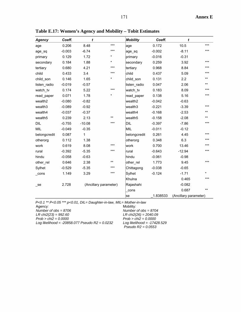
171 Annex E

Table E.17: Women’s Agency and Mobility – Tobit Estimates

Agency Coeff. t Mobility Coeff. t age 0.206 8.48 *** age 0.172 10.5 *** age_sq -0.003 -6.74 *** age_sq -0.002 -8.11 *** primary 0.129 1.72 * primary -0.016 -0.31 secondary 0.184 1.88 * secondary 0.259 3.92 *** tertiary 0.680 4.21 *** tertiary 0.968 8.84 *** child 0.433 3.4 *** child 0.437 5.09 *** child_son 0.146 1.65 * child_son 0.131 2.2 ** listen_radio -0.019 -0.57 listen_radio 0.047 2.06 ** watch_tv 0.174 5.22 *** watch_tv 0.183 8.09 *** read_paper 0.071 1.78 * read_paper 0.138 5.16 *** wealth2 -0.080 -0.82 wealth2 -0.042 -0.63 wealth3 -0.089 -0.92 wealth3 -0.221 -3.39 *** wealth4 -0.037 -0.37 wealth4 -0.168 -2.53 ** wealth5 0.239 2.13 ** wealth5 -0.158 -2.08 ** DIL -0.755 -10.08 *** DIL -0.397 -7.86 *** MIL -0.049 -0.35 MIL -0.011 -0.12 belongcredit 0.087 1 belongcredit 0.261 4.45 *** otherorg 0.112 1.38 otherorg 0.348 6.3 *** work 0.619 8.08 *** work 0.700 13.46 *** rural -0.392 -5.35 *** rural -0.643 -12.94 *** hindu -0.058 -0.63 hindu -0.061 -0.98 other_rel 0.646 2.38 ** other_rel 1.773 9.45 *** Sylhet -0.529 -5.35 *** Chittagong -0.038 -0.65 _cons 1.149 3.29 *** Sylhet -0.124 -1.71 * Khulna 0.465 *** _se 2.728 (Ancillary parameter) Rajashahi -0.082 _cons 0.687 ** se _1.838533 (Ancillary parameter)

P<0.1 ** P<0.05 *** p<0.01, DIL= Daughter-in-law, MIL= Mother-in-law Agency: Number of obs = 8706 LR chi2(23) = 992.60 Prob > chi2 = 0.0000 Log likelihood = -20858.077 Pseudo R2 = 0.0232

Mobility: Number of obs = 8704 LR chi2(26) = 2040.09 Prob > chi2 = 0.0000 Log likelihood = -17428.529 Pseudo R2 = 0.0553

Annex F 172

Annex F. Fertility

1. This annex presents analysis on fertility trends and determinants in the 1990s, and strategies for achieving continued fertility decline to accelerate achievement of a stable population. The first issue addressed is that of fertility trends in the 1990s. This issue is of policy importance, since there is a widespread perception that fertility decline leveled off in the 1990s, suggesting that the hitherto successful family planning program had run out of steam. In fact, as shown here, fertility decline continued throughout the 1990s, albeit at a slower rate than previously.

2. The regression model results feed directly into strategy formulation for maintaining fertility decline. First, the results clearly indicate that son preference is a barrier to reducing fertility. Experience in Bangladesh and elsewhere shows that son preference exerts itself more strongly as fertility falls, so that policies to address the problem, while not obvious, are required. The regression results show that, contrary to normal international patterns, age at marriage has limited potential to reduce fertility, why this is so is discussed. Hence, while desirable for other reasons, strategies to raise the age at marriage will have at best limited impact on fertility. It is proposed instead that attention should focus on high-fertility households.

What Has Been Happening to Fertility?

3. Following the rapid decline during the 1980s, DHS data suggest that fertility leveled off in the 1990s, declining slightly from 3.4 to 3.3 between 1993 and 1996, then remaining at that level until 1999.

4. It has been suggested that this slackening pace of fertility reduction comes from a tempo effect. Suppose during the 1980s women began postponing births while maintaining the number of children they had at the same level. Cohort fertility – the average number of children born to women of a particular age – would remain unchanged. But the total fertility rate is calculated using the synthetic cohort method, which is an average of the age-specific fertility rates of women currently alive. Hence, TFR will temporarily fall as a result of postponed births (because of the reduction in the age-specific fertility rate among those women postponing births) only to return to its original level when these women give birth in the next period (see Box F.1). Such a tempo effect in Bangladesh plausibly accelerated fertility decline in the 1980s, but served to counteract a continuing underlying decline in the early 1990s. If this argument is correct, then the fact that TFR stagnated rather than rose in the 1990s indeed implies that there were other changes taking place to exert a downward pressure on the TFR.

5. However, while there is evidence of such a tempo effect there is no need to rely on that to explain the claimed fertility plateau for a number of reasons. First, it has not been usual to rely on direct estimates of fertility to estimate fertility in the past, so it is not clear why they should be the reference point for the 1990s. Second, even if the direct estimates are used there are reasons to believe that fertility was underestimated in 1993/94 on account of displacement in birth reporting. But, third, if indirect estimates are used, they show both that the direct estimates underestimate fertility (particularly in 1993/94, reinforcing the previous point) and that fertility did continue to decline in the 1990s. These arguments are considered in turn.

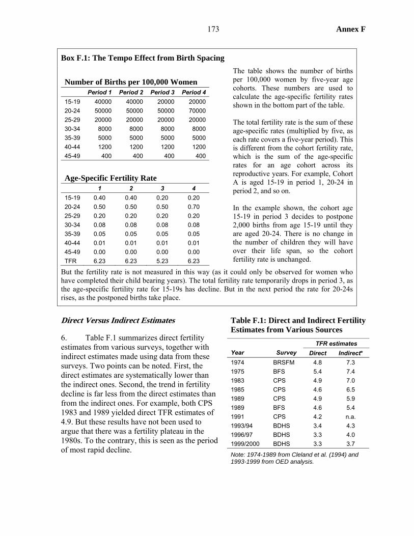
173 Annex F

Box F.1: The Tempo Effect from Birth Spacing Number of Births per 100,000 Women Period 1 Period 2 Period 3 Period 4 15-19 40000 40000 20000 20000 20-24 50000 50000 50000 70000 25-29 20000 20000 20000 20000 30-34 8000 8000 8000 8000 35-39 5000 5000 5000 5000 40-44 1200 1200 1200 1200 45-49 400 400 400 400

Age-Specific Fertility Rate 1 2 3 4 15-19 0.40 0.40 0.20 0.20 20-24 0.50 0.50 0.50 0.70 25-29 0.20 0.20 0.20 0.20 30-34 0.08 0.08 0.08 0.08 35-39 0.05 0.05 0.05 0.05 40-44 0.01 0.01 0.01 0.01 45-49 0.00 0.00 0.00 0.00 TFR 6.23 6.23 5.23 6.23

The table shows the number of births per 100,000 women by five-year age cohorts. These numbers are used to calculate the age-specific fertility rates shown in the bottom part of the table. The total fertility rate is the sum of these age-specific rates (multiplied by five, as each rate covers a five-year period). This is different from the cohort fertility rate, which is the sum of the age-specific rates for an age cohort across its reproductive years. For example, Cohort A is aged 15-19 in period 1, 20-24 in period 2, and so on. In the example shown, the cohort age 15-19 in period 3 decides to postpone 2,000 births from age 15-19 until they are aged 20-24. There is no change in the number of children they will have over their life span, so the cohort fertility rate is unchanged.

But the fertility rate is not measured in this way (as it could only be observed for women who have completed their child bearing years). The total fertility rate temporarily drops in period 3, as the age-specific fertility rate for 15-19s has decline. But in the next period the rate for 20-24s rises, as the postponed births take place.

Direct Versus Indirect Estimates

6. Table F.1 summarizes direct fertility estimates from various surveys, together with indirect estimates made using data from these surveys. Two points can be noted. First, the direct estimates are systematically lower than the indirect ones. Second, the trend in fertility decline is far less from the direct estimates than from the indirect ones. For example, both CPS 1983 and 1989 yielded direct TFR estimates of 4.9. But these results have not been used to argue that there was a fertility plateau in the 1980s. To the contrary, this is seen as the period of most rapid decline.

Table F.1: Direct and Indirect Fertility Estimates from Various Sources

TFR estimates Year Survey Direct Indirect* 1974 BRSFM 4.8 7.3 1975 BFS 5.4 7.4 1983 CPS 4.9 7.0 1985 CPS 4.6 6.5 1989 CPS 4.9 5.9 1989 BFS 4.6 5.4 1991 CPS 4.2 n.a. 1993/94 BDHS 3.4 4.3 1996/97 BDHS 3.3 4.0 1999/2000 BDHS 3.3 3.7

Note: 1974-1989 from Cleland et al. (1994) and 1993-1999 from OED analysis.

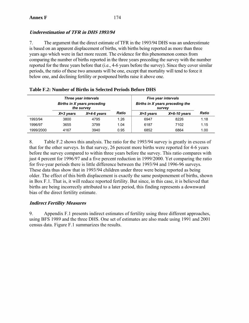
Annex F 174

Underestimation of TFR in DHS 1993/94

7. The argument that the direct estimate of TFR in the 1993/94 DHS was an underestimate is based on an apparent displacement of births, with births being reported as more than three years ago which were in fact more recent. The evidence for this phenomenon comes from comparing the number of births reported in the three years preceding the survey with the number reported for the three years before that (i.e., 4-6 years before the survey). Since they cover similar periods, the ratio of these two amounts will be one, except that mortality will tend to force it below one, and declining fertility or postponed births raise it above one.

Table F.2: Number of Births in Selected Periods Before DHS

Three year intervals Births in X years preceding

the survey

Five year intervals Births in X years preceding the

survey X=3 years X=4-6 years Ratio X=5 years X=6-10 years Ratio

1993/94 3800 4795 1.26 6947 8226 1.18 1996/97 3655 3799 1.04 6187 7102 1.15 1999/2000 4167 3940 0.95 6852 6864 1.00

8. Table F.2 shows this analysis. The ratio for the 1993/94 survey is greatly in excess of that for the other surveys. In that survey, 26 percent more births were reported for 4-6 years before the survey compared to within three years before the survey. This ratio compares with just 4 percent for 1996/97 and a five percent reduction in 1999/2000. Yet comparing the ratio for five-year periods there is little difference between the 1993/94 and 1996-96 surveys. These data thus show that in 1993/94 children under three were being reported as being older. The effect of this birth displacement is exactly the same postponement of births, shown in Box F.1. That is, it will reduce reported fertility. But since, in this case, it is believed that births are being incorrectly attributed to a later period, this finding represents a downward bias of the direct fertility estimate.

Indirect Fertility Measures

9. Appendix F.1 presents indirect estimates of fertility using three different approaches, using BFS 1989 and the three DHS. One set of estimates are also made using 1991 and 2001 census data. Figure F.1 summarizes the results.

175 Annex F

3

4

5

6

7

8

1980 1985 1990 1995 2000

Tota

l fer

tility

rate


Regression method

Rele: census data

Rele: survey data

Figure F.1 Indirect Estimates of TFR

10. The data shown here confirm that direct methods overestimate fertility. This gap is largest for 1993/94, which supports the argument that birth displacement exacerbated underestimation in that year. The results also show that fertility continued to decline during the 1990s, albeit at a slower rate than had been the case from 1989-93.

Summary

11. Three arguments have been presented to counter the commonly held view that there was a fertility plateau in Bangladesh in the 1990s. This finding matters, since the perceived plateau gave weight to the view that family planning services were becoming moribund and could not make additional inroads into fertility. The fact that fertility was being reduced points to the continuing success of these programs. Nonetheless, it is the case that the rate of fertility reduction was slowing down, suggesting that thought does need be given to strategy for attaining the goal of a stable population.

Modeling Fertility Determinants

12. Table F.3 presents the results of regression models of two dependent variables which proxy for fertility: (1) whether a woman desires to have more children and (2) whether a woman has had a birth in the last three years. Some of the expected patterns emerge here: all regions have lower fertility than Sylhet, non-Muslims have lower fertility, women with more children are less likely to desire another child and older women are less likely to have had a

Annex F 176

child in the last three years or to desire another. Working women have lower fertility, which may reflect the effect of women’s agency. Some of the other results require more comment.

13. First, the age at marriage is significantly positively related to the two fertility measures, a result that is robust to different model specifications. This finding is contrary to the conventional wisdom that increasing age at marriage is a driver of lower fertility, as indeed has been the case in many countries (including quite probably Bangladesh in the past). However, as discussed in more detail below, since fertility is already low, there is limited possibility for increasing age at marriage to reduce fertility – the effect is rather to postpone births (which will, as explained above, create a tempo effect which temporarily accelerates the rate of fertility decline). Hence, women who have married later are more likely to want more children and to have had a child in the last three years.

14. Second, the level of education has the expected effect on the desire for more children – more educated women are less likely to want another child. But there is the opposite relationship for women who have had a child in the last three years, those women having reached at least grade 6 are more likely to have had a child in the last three years, and those at grade 10 and above even more likely to have done so. This result once again reflects the marriage postponement effect – women attending school after the onset of their reproductive years are postponing births rather than having fewer than the (already low) average.

15. Third, there is considerable evidence of son preference. This preference is picked up by the four interactive variables used in the final regression. A woman is more likely to have had a child in the last four years if all her children are girls (although this effect is mitigated somewhat if she has a lot of them), and less likely to if she already has a son.

16. Fourth, access to electricity has an unexpected, though insignificant, positive impact on the desire to have more children. However, the coefficient becomes negative (though still insignificant) once the media variables are removed. This result shows that the effect electricity has on lowering fertility is by facilitating access to media, notably TV, which has a significant fertility reducing effect when included. This variable is thus a measure of the impact of IEC through one specific channel.

17. Finally, it might be expected that the survey dummy coefficients would be negative, showing an “autonomous” downward trend in fertility by factors not included in the survey. This pattern is present, though not significant, for the “desire more children regression.” But the result does not appear for the child in last three years result. Rather than evidence of such a downward trend, this result reinforces the argument of birth displacement in the 1993/94 survey.

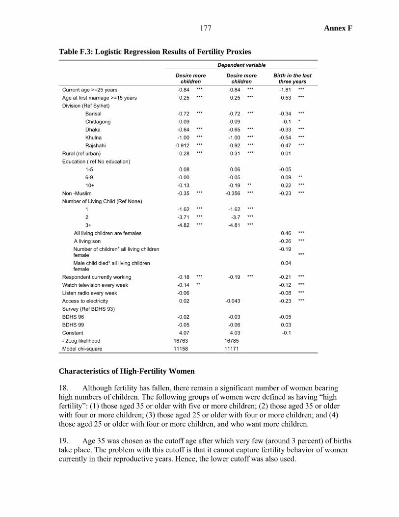
177 Annex F

Table F.3: Logistic Regression Results of Fertility Proxies Dependent variable

Desire more children

Desire more children

Birth in the last three years

Current age >=25 years -0.84 *** -0.84 *** -1.81 *** Age at first marriage >=15 years 0.25 *** 0.25 *** 0.53 *** Division (Ref Sylhet) Barisal -0.72 *** -0.72 *** -0.34 *** Chittagong -0.09 -0.09 -0.1 * Dhaka -0.64 *** -0.65 *** -0.33 *** Khulna -1.00 *** -1.00 *** -0.54 *** Rajshahi -0.912 *** -0.92 *** -0.47 *** Rural (ref urban) 0.28 *** 0.31 *** 0.01 Education ( ref No education) 1-5 0.08 0.06 -0.05 6-9 -0.00 -0.05 0.09 ** 10+ -0.13 -0.19 ** 0.22 *** Non -Muslim -0.35 *** -0.356 *** -0.23 *** Number of Living Child (Ref None) 1 -1.62 *** -1.62 *** 2 -3.71 *** -3.7 *** 3+ -4.82 *** -4.81 *** All living children are females 0.46 *** A living son -0.26 *** Number of children* all living children

female

-0.19

*** Male child died* all living children

female

0.04

Respondent currently working -0.18 *** -0.19 *** -0.21 *** Watch television every week -0.14 ** -0.12 *** Listen radio every week -0.06 -0.08 *** Access to electricity 0.02 -0.043 -0.23 *** Survey (Ref BDHS 93) BDHS 96 -0.02 -0.03 -0.05 BDHS 99 -0.05 -0.06 0.03 Constant 4.07 4.03 -0.1 - 2Log likelihood 16763 16785 Model chi-square 11158 11171

Characteristics of High-Fertility Women

18. Although fertility has fallen, there remain a significant number of women bearing high numbers of children. The following groups of women were defined as having “high fertility”: (1) those aged 35 or older with five or more children; (2) those aged 35 or older with four or more children; (3) those aged 25 or older with four or more children; and (4) those aged 25 or older with four or more children, and who want more children.

19. Age 35 was chosen as the cutoff age after which very few (around 3 percent) of births take place. The problem with this cutoff is that it cannot capture fertility behavior of women currently in their reproductive years. Hence, the lower cutoff was also used.

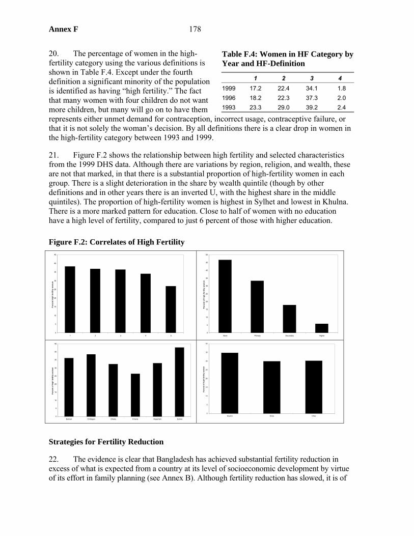
Annex F 178

20. The percentage of women in the high-fertility category using the various definitions is shown in Table F.4. Except under the fourth definition a significant minority of the population is identified as having “high fertility.” The fact that many women with four children do not want more children, but many will go on to have them represents either unmet demand for contraception, incorrect usage, contraceptive failure, or that it is not solely the woman’s decision. By all definitions there is a clear drop in women in the high-fertility category between 1993 and 1999.

21. Figure F.2 shows the relationship between high fertility and selected characteristics from the 1999 DHS data. Although there are variations by region, religion, and wealth, these are not that marked, in that there is a substantial proportion of high-fertility women in each group. There is a slight deterioration in the share by wealth quintile (though by other definitions and in other years there is an inverted U, with the highest share in the middle quintiles). The proportion of high-fertility women is highest in Sylhet and lowest in Khulna. There is a more marked pattern for education. Close to half of women with no education have a high level of fertility, compared to just 6 percent of those with higher education.

Figure F.2: Correlates of High Fertility

0

5

10

15

20

25

30

35

40

45

1 2 3 4 5

Per

cent

hig

h fe

rtili

ty w

omen

0

5

10

15

20

25

30

35

40

45

50

None Primary Secondary Higher

Perc

ent o

f hig

h fe

rilit

y w

omen

0

5

10

15

20

25

30

35

40

45

Barisal Chittagon Dhaka Khulna Rajashahi Sylhet

Perc

ent o

f hig

h fe

rtili

ty w

omen

0

5

10

15

20

25

30

35

40

Muslim Hindu Other

Perc

ent o

f hig

ht fe

rility

wom

en

Strategies for Fertility Reduction

22. The evidence is clear that Bangladesh has achieved substantial fertility reduction in excess of what is expected from a country at its level of socioeconomic development by virtue of its effort in family planning (see Annex B). Although fertility reduction has slowed, it is of

Table F.4: Women in HF Category by Year and HF-Definition

1 2 3 4 1999 17.2 22.4 34.1 1.8 1996 18.2 22.3 37.3 2.0 1993 23.3 29.0 39.2 2.4

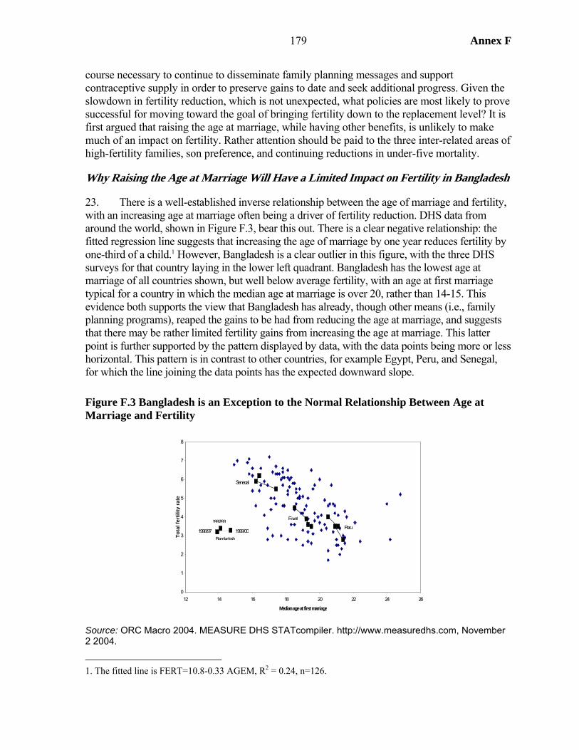
179 Annex F

course necessary to continue to disseminate family planning messages and support contraceptive supply in order to preserve gains to date and seek additional progress. Given the slowdown in fertility reduction, which is not unexpected, what policies are most likely to prove successful for moving toward the goal of bringing fertility down to the replacement level? It is first argued that raising the age at marriage, while having other benefits, is unlikely to make much of an impact on fertility. Rather attention should be paid to the three inter-related areas of high-fertility families, son preference, and continuing reductions in under-five mortality.

Why Raising the Age at Marriage Will Have a Limited Impact on Fertility in Bangladesh

23. There is a well-established inverse relationship between the age of marriage and fertility, with an increasing age at marriage often being a driver of fertility reduction. DHS data from around the world, shown in Figure F.3, bear this out. There is a clear negative relationship: the fitted regression line suggests that increasing the age of marriage by one year reduces fertility by one-third of a child.1 However, Bangladesh is a clear outlier in this figure, with the three DHS surveys for that country laying in the lower left quadrant. Bangladesh has the lowest age at marriage of all countries shown, but well below average fertility, with an age at first marriage typical for a country in which the median age at marriage is over 20, rather than 14-15. This evidence both supports the view that Bangladesh has already, though other means (i.e., family planning programs), reaped the gains to be had from reducing the age at marriage, and suggests that there may be rather limited fertility gains from increasing the age at marriage. This latter point is further supported by the pattern displayed by data, with the data points being more or less horizontal. This pattern is in contrast to other countries, for example Egypt, Peru, and Senegal, for which the line joining the data points has the expected downward slope.

Figure F.3 Bangladesh is an Exception to the Normal Relationship Between Age at Marriage and Fertility

Source: ORC Macro 2004. MEASURE DHS STATcompiler. http://www.measuredhs.com, November 2 2004.

1. The fitted line is FERT=10.8-0.33 AGEM, R2 = 0.24, n=126.

0

1

2

3

4

5

6

7

8

12 14 16 18 20 22 24 26

Median age at first marriage

Tota

l fer

tility

rate

Bangladesh1996/97

1992/93

1999/00

Egypt

Peru

Senegal

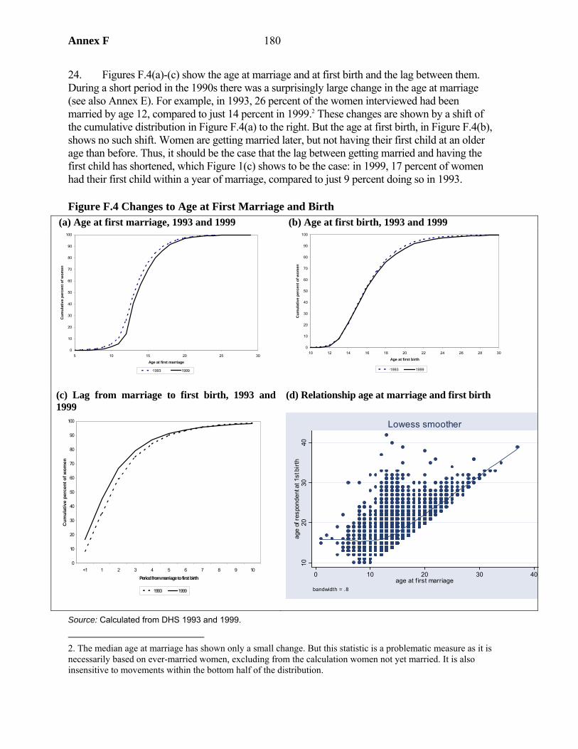
Annex F 180

24. Figures F.4(a)-(c) show the age at marriage and at first birth and the lag between them. During a short period in the 1990s there was a surprisingly large change in the age at marriage (see also Annex E). For example, in 1993, 26 percent of the women interviewed had been married by age 12, compared to just 14 percent in 1999.2 These changes are shown by a shift of the cumulative distribution in Figure F.4(a) to the right. But the age at first birth, in Figure F.4(b), shows no such shift. Women are getting married later, but not having their first child at an older age than before. Thus, it should be the case that the lag between getting married and having the first child has shortened, which Figure 1(c) shows to be the case: in 1999, 17 percent of women had their first child within a year of marriage, compared to just 9 percent doing so in 1993.

Figure F.4 Changes to Age at First Marriage and Birth (a) Age at first marriage, 1993 and 1999 (b) Age at first birth, 1993 and 1999

(c) Lag from marriage to first birth, 1993 and 1999

(d) Relationship age at marriage and first birth

1020

3040

age

of re

spon

dent

at 1

st b

irth

0 10 20 30 40age at f irst marriage

bandwidth = .8

Lowess smoother

Source: Calculated from DHS 1993 and 1999.

2. The median age at marriage has shown only a small change. But this statistic is a problematic measure as it is necessarily based on ever-married women, excluding from the calculation women not yet married. It is also insensitive to movements within the bottom half of the distribution.

0

10

20

30

40

50

60

70

80

90

100

5 10 15 20 25 30

Age at first marriage

Cum

ulat

ive

perc

ent o

f wom

en

1993 1999

0

10

20

30

40

50

60

70

80

90

100

10 12 14 16 18 20 22 24 26 28 30

Age at first birth

Cum

ulat

ive

perc

ent o

f wom

en

1993 1999

0

10

20

30

40

50

60

70

80

90

100

<1 1 2 3 4 5 6 7 8 9 10

Period from marriage to first birth

Cum

ulat

ive

perc

ent o

f wom

en

1993 1999

181 Annex F

25. Figure 1(d), which shows the scatter plot of age at first birth against age at marriage, digs a bit deeper into what is going on here. The plot is fitted with a locally weighted regression line, which shows there is no relationship between age of marriage and age at first birth (i.e., the regression line is flat) up to about 13 years of age.3 Close to 20 percent of ever-married women in the 1990s had married by 12 and 40 percent by 13. But, as the graph shows, increasing the age at marriage within this age range will have no effect at all on the age at first birth. Girls getting married below age 13 are generally considered to be below reproductive age and only exceptionally bear children (only 4 percent of births are to girls aged 13 and younger). Second, the slope of the line, which is constant after the structural break at around 13 years, is less than 1 (it is 0.8, see footnote 3). Hence, an increase in the age of marriage of one year leads to a one less a one year increase. This mean that as the age at marriage increases the absolute gap between marriage and first birth declines. The regression results suggest this gap is on average 2.7 years for a woman marrying at 15 but only 1.8 years for one marrying at 20. This is precisely the phenomenon shown in panels (a) and (c) of Figure F.4 – as the age at marriage increases the interval to first birth declines.

26. The point being made above is that delaying marriage only has a limited effect of delaying the onset of a woman’s reproductive life.4 It has, on average, no effect at all for women marrying at 13 or less. And it has a muted effect on older women.

27. It is usually argued that delaying marriage reduces fertility since a woman starts reproduction later, and so has less time to achieve her reproductive potential. But in Bangladesh the majority of women are having three or four children during their reproductive lives. This is quite possible to achieve if childbearing starts at 20 rather 15. Hence, even if delaying marriage delayed first births, which it does to only a limited extent, it still would not affect the total number of children they have during their lifetime.

Strategies to Reduce Fertility: Addressing High-Fertility Households, Son Preference, and High Mortality

28. As shown above, one-third of all women aged 25 have four or more children. There seems greater potential in persuading these families to have 3 children than in persuading those having 2-3 children to have fewer. That son preference is a barrier to fertility decline in Bangladesh has been argued elsewhere (Chowdury and Bairagi 1990; Bairagim 1996; and Khan and Khanum 2000), and is supported in the regression results presented above. Reducing son preference would hence have a beneficial impact on fertility. This is easier said than done, son preference is a deeply engrained cultural tradition, exacerbated by the spread and escalation of dowry.5 Strategies which may be adopted include Behavior Change

3. Alternatively, OLS can be used with a spline function, which gives age_fb= 5.24 + 0.83 age_marr + 10.2 dum – 0.82 sldum, where dum=1 for women married at 13 or less, and sldum is the slope dummy for that variable for these women.

4. Of course, any delay will have a temporary tempo effect on the TFR.

5. Until some generations ago, bridewealth was practiced in Bangladesh, but has now been commonly replaced by dowry which was previously only found among Hindus. The former practice is consistent with Islam whereas the latter is not.

Annex F 182

Communication, particularly including work with religious authorities, expanding female education, and employment and income-generating opportunities for women. These last two areas of already sizeable programs in Bangladesh.

29. Bangladesh has followed international norms in that fertility decline has been linked to declining under-five mortality. There remain pockets of high mortality, especially in Sylhet where use of health services is low. Concerted efforts to increase immunization coverage and other interventions to reduce mortality can be expected to have an impact on fertility in these areas.

183 Annex F

APPENDIX 1. INDIRECT ESTIMATES OF FERTILITY IN THE 1990S

1. This appendix provides indirect estimates of fertility in Bangladesh for the 1990s using three methods: Rele method, Proximate Determinant method (Bongaarts decomposition), and the regression method. The data for the analysis are taken from BFS 1989 and the three DHS surveys, and, for one set of calculations, census data.

Rele Method

2. This method infers fertility levels from child-woman ratios (CWR), utilizing the close linear relationship between the CWR and the gross reproduction rate (GRR)6 shown to exist at any given level of mortality (measured by life expectancy, e0

0). Rele (1976) provides the parameters required for implementation of the approach.7 Using these coefficients, GRR is estimated from CWR using suitable values of e0

0 in a given population and then applying the sex-ratio at birth estimate to obtain TFR from GRR.

3. The method uses two types of CWR in estimating GRR, namely, children aged 0-4 years divided by women aged 15-49 (CWR1) and children aged 5-9 divided by women aged 20-54 (CWR2). The e0

0 value used corresponds to the period when the children in the CWR were born. The fertility estimates also refer to the same period viz., estimates obtained through using CWR1 produces an estimate for five years preceding the census/survey and that with CWR2 produces for 5 to 10 years preceding that.

4. This method has certain strength and weaknesses. Among the former, the estimated fertility is insensitive to the errors in e0

0, so that an approximate value of e00 gives a fairly

accurate estimate of fertility. Among the weaknesses, the derived fertility estimates depend on the accuracy of CWR. In developing countries, due to errors in age reporting, notably exaggeration of age at young ages and underreporting of very young children, the reported age distributions are often distorted. To overcome this problem it was initially suggested to average the two rates obtained from the two CWRs and arrive at a decadal estimate (Rele 1976). Also, one may use smoothed age data. But this procedure has some disadvantage as estimates with the smoothed age distribution are influenced by the particular method used in smoothing the age data.

5. Rele (1987) refines the method for situations more typical in some developing countries, including India. The refined method requires two or more successive censuses preferably with a 10 year gap between them and use of weights8 derived on the basis of extent of under-enumeration/over–enumeration of two types of CWRs to adjust preliminary

6. The GRR is the average number of daughters that would be born alive to a woman (or group of women) during her lifetime based on currently prevailing age if she passed through her childbearing years conforming to the age-specific fertility rates.

7. GRR= a + b CRW, where a and b are given in Rele (1976). The TFR= GRR x2.05 (assumed sex ratio at birth).

8. Suggested weights to arrive at a final estimates are 0.7 for GRR obtained from CWR2 and 0.3 for GRR obtained from CWR1.

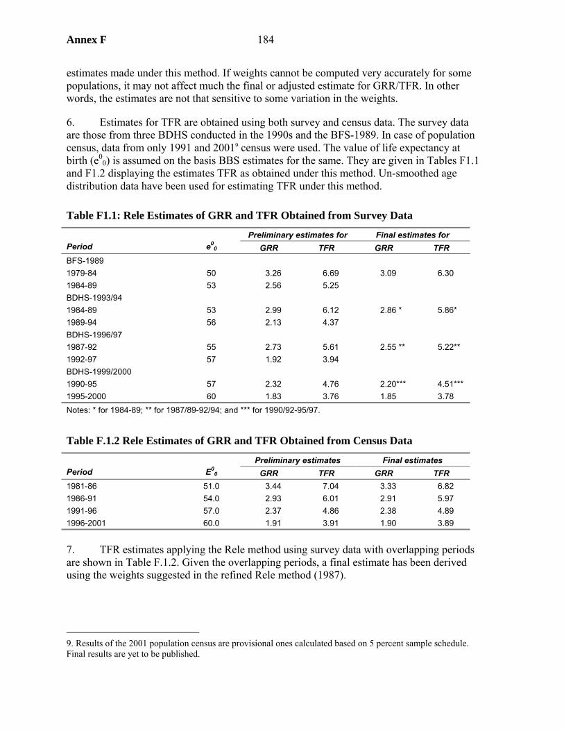
Annex F 184

estimates made under this method. If weights cannot be computed very accurately for some populations, it may not affect much the final or adjusted estimate for GRR/TFR. In other words, the estimates are not that sensitive to some variation in the weights.

6. Estimates for TFR are obtained using both survey and census data. The survey data are those from three BDHS conducted in the 1990s and the BFS-1989. In case of population census, data from only 1991 and 20019 census were used. The value of life expectancy at birth (e0

0) is assumed on the basis BBS estimates for the same. They are given in Tables F1.1 and F1.2 displaying the estimates TFR as obtained under this method. Un-smoothed age distribution data have been used for estimating TFR under this method.

Table F1.1: Rele Estimates of GRR and TFR Obtained from Survey Data

Preliminary estimates for Final estimates for Period e0

0 GRR TFR GRR TFR BFS-1989 1979-84 50 3.26 6.69 3.09 6.30 1984-89 53 2.56 5.25 BDHS-1993/94 1984-89 53 2.99 6.12 2.86 * 5.86* 1989-94 56 2.13 4.37 BDHS-1996/97 1987-92 55 2.73 5.61 2.55 ** 5.22** 1992-97 57 1.92 3.94 BDHS-1999/2000 1990-95 57 2.32 4.76 2.20*** 4.51*** 1995-2000 60 1.83 3.76 1.85 3.78 Notes: * for 1984-89; ** for 1987/89-92/94; and *** for 1990/92-95/97.

Table F.1.2 Rele Estimates of GRR and TFR Obtained from Census Data

Preliminary estimates Final estimates Period E0

0 GRR TFR GRR TFR 1981-86 51.0 3.44 7.04 3.33 6.82 1986-91 54.0 2.93 6.01 2.91 5.97 1991-96 57.0 2.37 4.86 2.38 4.89 1996-2001 60.0 1.91 3.91 1.90 3.89

7. TFR estimates applying the Rele method using survey data with overlapping periods are shown in Table F.1.2. Given the overlapping periods, a final estimate has been derived using the weights suggested in the refined Rele method (1987).

9. Results of the 2001 population census are provisional ones calculated based on 5 percent sample schedule. Final results are yet to be published.

185 Annex F

Proximate Determinant Method

8. Davis and Blake (1956) were the first investigators to develop a framework outlining the intermediate fertility variables. That seminal work identified 11 intermediate variables through which fertility gets affected in a population. Later on, Bongaaarts (1978) revised this framework incorporating only 8 of them, which he termed as proximate determinants of fertility. As he suggested, each of these eight variables directly influences the fertility and they together determine the level of fertility in a population. However, using the data from both developed and developing countries Bongaarts and Potter (1983) observed that 96 percent of the variance in total fertility rates could be explained by four principal proximate determinants, namely, marriage, contraception, induced abortion, and lactational infecundability. The other four, which can be disregarded, are: frequency of intercourse, sterility, spontaneous intrauterine mortality, and duration of the fertile period. These last four factors all relate to the natural fertility.

9. The key contribution of the Bongaarts framework is to set up the procedures for parceling out the effects on fertility of different proximate variables. The forces of each of the intermediate variables in the Bongaarts framework is measured by an index ‘C’ that varies from zero to one. When it is zero, none of the potential for fertility is translated into births. When it is 1.0, the controls exerts no restraining effect whatsoever.

10. In Bongaarts’ framework the total fertility rate (TFR) in a population is expressed as the product of four indexes measuring the fertility inhibiting effect of four principal intermediate variables and the total fecundity rate (TF). The total fecundity rate is the average number of live births expected among women who during their entire reproductive period remain married, do not use contraception, do not have any induced abortion, and do not breastfeed their children. The TF does not vary much between populations, lying between 13 and 17 births per woman with a standard value of 15.3 (Bongaarts and Potter 1983).

11. The following equation summarizes the basic structure of the Bongaarts model by relating the fertility measures to the proximate determinants:

TFR= Cm x Cc x Ci x Ca x TF

Where Cm is the index of marriage, Cc is the index of contraception, Ca is the index of induced abortion, and Ci is the index of lactational infecundability. Each index measures the extent to which fertility is reduced from the maximal levels by specified proximate determinants. The indexes are measured as follows:

g(a)g(a)m(a)Cm ∑

×=

Where m (a) = age specific proportions currently married among female and g(a) = age specific marital fertility rate.

Cc = 1-1.08 x u x e

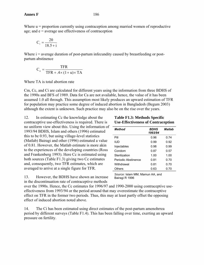
Annex F 186

Where u = proportion currently using contraception among married women of reproductive age; and e = average use effectiveness of contraception

i 18.520Ci +

=

Where i = average duration of post-partum infecundity caused by breastfeeding or post-partum abstinence

TA u)(1 .4 TFRTFRCa ×+×+

=

Where TA is total abortion rate

Cm, Cc, and Ci are calculated for different years using the information from three BDHS of the 1990s and BFS of 1989. Data for Ca are not available, hence, the value of it has been assumed 1.0 all through. This assumption most likely produces an upward estimation of TFR for population may practice some degree of induced abortion in Bangladesh (Begum 2003) although the extent is unknown. Such practice may also be on the rise over the years.

12. In estimating Cc the knowledge about the contraceptive use-effectiveness is required. There is no uniform view about this. Using the information of 1993/94 BDHS, Islam and others (1996) estimated this to be 0.93, but using village-level statistics (Matlab) Bairagi and other (1996) estimated a value of 0.81. However, the Matlab estimate is more akin to the experiences of the developing countries (Ross and Frankenberg 1993). Here Cc is estimated using both sources (Table F1.3) giving two Cc estimates and, consequently, two TFR estimates, which are averaged to arrive at a single figure for TFR.

13. However, the BDHS have shown an increase in the discontinuation rate of contraceptive methods over the 1990s. Hence, the Cc estimates for 1996/97 and 1990-2000 using contraceptive use-effectiveness from 1993/94 or the period around that may overestimate the contraceptive effect on TFR in the former two periods. Thus, this may at least partly offset the opposing effect of induced abortion noted above.

14. The Ci has been estimated using direct estimates of the post-partum amenohrrea period by different surveys (Table F1.4). This has been falling over time, exerting an upward pressure on fertility.

Table F1.3: Methods Specific Use-Effectiveness of Contraception

Method BDHS 1993/94

Matlab

Pill 0.96 0.74 IUD 0.99 0.92 Injectables 0.98 0.99 Condom 0.87 0.57 Sterilization 1.00 1.00 Periodic Abstinence 0.81 0.70 Withdrawal 0.81 0.70 Others 0.63 0.70

Source: Islam MM, Mamun AA, and Bairagi R 1996

187 Annex F

15. The values of Cm, Cc, and Ci as estimated for different periods are presented in Table F1.5, together with the corresponding TFR. TFR is shown to have continued to fall during the 1990s, with the bulk of the decline coming from increased contraceptive usage. As noted, Ci exerted a countervailing tendency.

Table F1.5: Estimated Index Values of the Proximate Determinants Cc

Year Cm

Using BDHS use-

effectiveness

Using Matlab use-

effectiveness Ci Cm x Cc

x Ci * TFR* BFS 1989 .826 .695 .730 .658 .387 5.99 BDHS 1993/94 .761 .550 .610 .667 .294 4.50 BDHS 1996/97 .756 .503 .573 .680 .276 4.23 BDHS 1999-2000 .745 .466 .545 .714 .269 4.11 % change 89-99 -9.8 -32.9 -25.3 8.5 -30.5 -31.4 Share 32.2 95.6* -27.9 100.0 Notes: * Calculated using average of two Ccs.. Growth rate of TFR differs from that of product term due to rounding.

Regression Method

16. From international comparisons of the family planning program performance and fertility change Blanc (1990) has derived a set of regression equations that can be used to predict TFR from the information on CPR. Blanc proposed five regression equations. However, to arrive at a single value of TFR the average of five TFR values is suggested. Past users of this method have argued that this method is likely to produce an underestimation of TFR in a country like Bangladesh (Kantner and Frankenberg 1986; Kantner and Noor 1992), and suggested that estimates obtained through this procedure may be treated as the lower-bound estimates. The TFR estimation formulae under this method are as follows and to arrive at a single value for the TFR five different estimates obtained under five different formulae are average out.

TFR= 7.30 – (6.42 * CPR) TFR= 6.83 – (6.20 * CPR) TFR= 7.38 – (7.20 * CPR) TFR= 7.28 – (6.55 * CPR) TFR= 7.15 – (6.56 * CPR)

The results are presented in the next section, alongside those of the other methods.

Table F1.4: Estimated Duration of Post-Partum Amenorrhoea (in months)

Period Duration (months)

1989 11.9 1993/94 11.5 1996/97 10.9 1999-2000 9.5

Source: Survey Reports

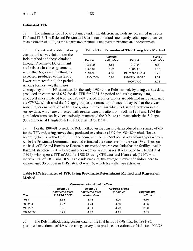
Annex F 188

Estimated TFR

17. The estimates for TFR as obtained under the different methods are presented in Tables F1.6 and F1.7. The Rele and Proximate Determinant methods are mainly relied upon to arrive at an estimate of TFR, as the Regression method is believed to produce an underestimate.

18. The estimates obtained using census and survey data under the Rele method and those obtained through Proximate Determinant methods are in close agreement, while the Regression method, as expected, produced consistently lower estimates for all the periods. Among former two, the major discrepancy is for TFR estimates for the early 1980s. The Rele method, by using census data, produced an estimate of 6.82 for the TFR for 1981-86 period and, using survey data, produced an estimate of 6.30 for 1979-84 period. Both estimates are obtained using primarily the CWR2, which used the 5-9 age group as the numerator, hence it may be that there was some higher enumeration of this age group in the census which is less of a problem in the survey data, which are collected with greater care and attention. Both in 1961 and 1974 the population censuses have excessively enumerated the 0-9 age and particularly the 5-9 age (Government of Bangladesh 1961; Begum 1976, 1990).

19. For the 1986-91 period, the Rele method, using census data, produced an estimate of 6.0 for the TFR and, using survey data, produced an estimate of 5.9 for 1984-89 period. Hence, according to this method the TFR in the country in the 1987-89 period was around 6 per women while the Proximate Determinant method estimated the same level for the year 1989. Thus, on the basis of Rele and Proximate Determinants method we can conclude that the fertility level in Bangladesh before 1990 was around 6 per woman. A similar result was found by Cleland et al. (1994), who report a TFR of 5.86 for 1988-89 using CPS data, and Islam et al. (1996), who report a TFR of 5.83 using BFS. As a crude measure, the average number of children born to women aged 35 or over in DHS 1992/93 was 5.9, which fits with these estimates.

Table F1.7: Estimates of TFR Using Proximate Determinant Method and Regression Method


Year

Using Cc estimated from 1993/94 BDHS

Using Cc estimated from

Matlab data

Average of two estimates Regression

method 1989 5.85 6.14 5.99 5.16 1993/94 4.27 4.74 4.50 4.25 1996/97 3.96 4.51 4.23 3.96 1999-2000 3.79 4.43 4.11 3.65

20. The Rele method, using census data for the first half of 1990s viz., for 1991-96, produced an estimate of 4.9 while using survey data produced an estimate of 4.51 for 1990/92-

Table F1.6: Estimates of TFR Using Rele Method

Period Census

estimates Period Survey

estimates 1981-86 6.82 1979-84 6.3 1986-91 5.97 1984-89 5.86 1991-96 4.89 1987/89-1992/94 5.22 1996-2000 3.93 1990/92-1995/97 4.51 1995-2000 3.78

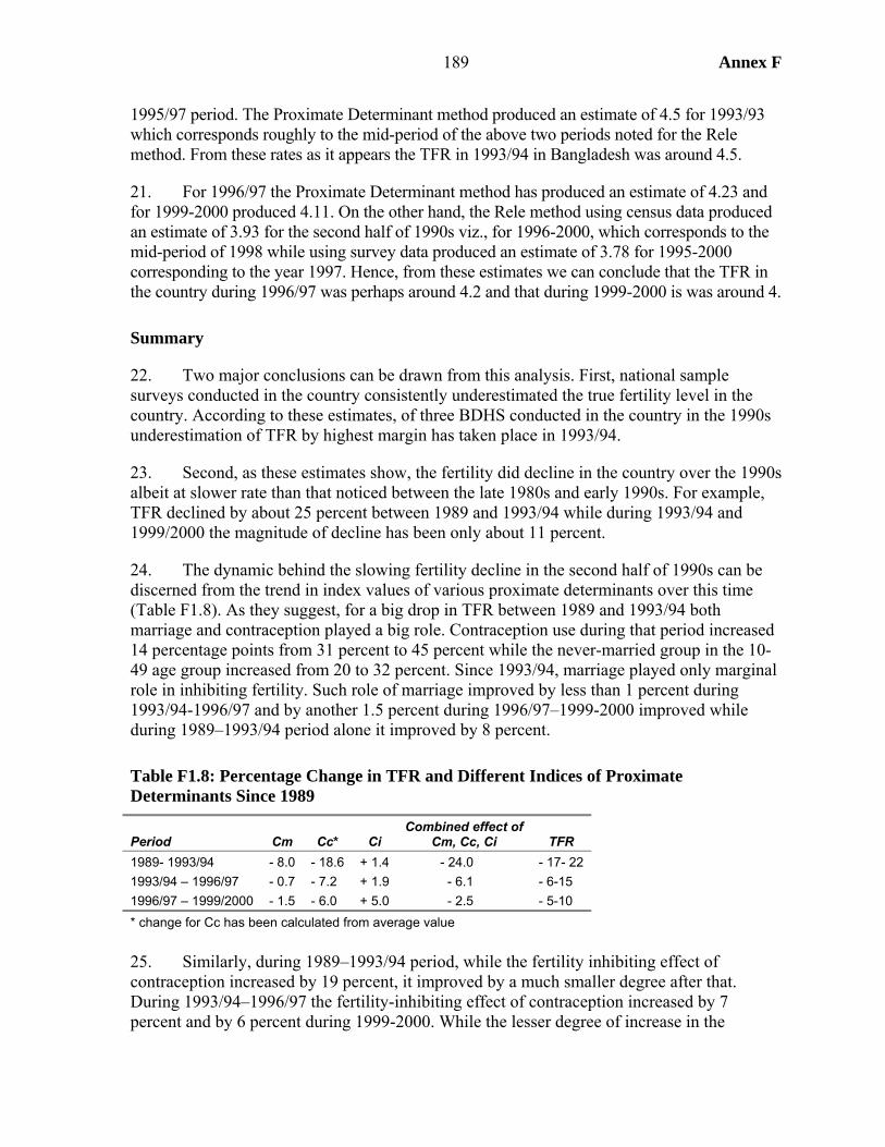
189 Annex F

1995/97 period. The Proximate Determinant method produced an estimate of 4.5 for 1993/93 which corresponds roughly to the mid-period of the above two periods noted for the Rele method. From these rates as it appears the TFR in 1993/94 in Bangladesh was around 4.5.

21. For 1996/97 the Proximate Determinant method has produced an estimate of 4.23 and for 1999-2000 produced 4.11. On the other hand, the Rele method using census data produced an estimate of 3.93 for the second half of 1990s viz., for 1996-2000, which corresponds to the mid-period of 1998 while using survey data produced an estimate of 3.78 for 1995-2000 corresponding to the year 1997. Hence, from these estimates we can conclude that the TFR in the country during 1996/97 was perhaps around 4.2 and that during 1999-2000 is was around 4.

Summary

22. Two major conclusions can be drawn from this analysis. First, national sample surveys conducted in the country consistently underestimated the true fertility level in the country. According to these estimates, of three BDHS conducted in the country in the 1990s underestimation of TFR by highest margin has taken place in 1993/94.

23. Second, as these estimates show, the fertility did decline in the country over the 1990s albeit at slower rate than that noticed between the late 1980s and early 1990s. For example, TFR declined by about 25 percent between 1989 and 1993/94 while during 1993/94 and 1999/2000 the magnitude of decline has been only about 11 percent.

24. The dynamic behind the slowing fertility decline in the second half of 1990s can be discerned from the trend in index values of various proximate determinants over this time (Table F1.8). As they suggest, for a big drop in TFR between 1989 and 1993/94 both marriage and contraception played a big role. Contraception use during that period increased 14 percentage points from 31 percent to 45 percent while the never-married group in the 10-49 age group increased from 20 to 32 percent. Since 1993/94, marriage played only marginal role in inhibiting fertility. Such role of marriage improved by less than 1 percent during 1993/94-1996/97 and by another 1.5 percent during 1996/97–1999-2000 improved while during 1989–1993/94 period alone it improved by 8 percent.

Table F1.8: Percentage Change in TFR and Different Indices of Proximate Determinants Since 1989

Period Cm Cc* Ci Combined effect of

Cm, Cc, Ci TFR 1989- 1993/94 - 8.0 - 18.6 + 1.4 - 24.0 - 17- 22 1993/94 – 1996/97 - 0.7 - 7.2 + 1.9 - 6.1 - 6-15 1996/97 – 1999/2000 - 1.5 - 6.0 + 5.0 - 2.5 - 5-10 * change for Cc has been calculated from average value 25. Similarly, during 1989–1993/94 period, while the fertility inhibiting effect of contraception increased by 19 percent, it improved by a much smaller degree after that. During 1993/94–1996/97 the fertility-inhibiting effect of contraception increased by 7 percent and by 6 percent during 1999-2000. While the lesser degree of increase in the

Annex F 190

contraception use after 1993/94 compared to 1989-1993/94 may in part be responsible for this, there is also evidence that in latter part of the 1990s contraception use relied more on relatively less-effective methods and the use-effectiveness of the method experienced some decline during this period.

26. Throughout this period the role of post-partum infecundability has been in opposite direction viz., it favored fertility increase. Not only this, such role of it rather increased noticeably over time offsetting part of the fertility-inhibiting effect exerted by other proximate determinants. During the 1989–1993/94 period the fertility inhibiting effect of Ci slackened by 1.4 percent, it slackened by another 1.9 percent during the 193/94–1996/97 period and another 5 percent during 1996/97–1999/2000.

27. The outcome of all these effects has been continuous weakening of collective strength of the fertility-inhibiting effect of various proximate determinants. During the 1989–1993/94 period above mentioned three proximate determinants viz., Cm, Cc, and Ci together could improve their fertility depressing effect by another 24 percent. While they could continue improving such effect throughout the rest of 1990s, they could do so only to lesser degree. During 1993/94–1996/97 such improvement has been of another 6 percent and during 1996/97 and 1999/2000 it improved by another 2.5 percent.

191 Annex G

Annex G. Analysis of BINP’s Community-Based Nutrition Component

1. The Community-Based Nutrition Component, the central component of BINP, focused on growth monitoring combined with nutritional counseling and food supplementation. The impact of the component has been studied in an independent evaluation conducted for the project (Karim et al. 2003), by Save the Children in their report Thin on the Ground (Save the Children 2003), in an evaluation commissioned by GoB’s Implementation, Monitoring and Evaluation Department (Haider et al. 2004), and in research carried out under the supervision of Professor Mascie-Taylor at the University of Cambridge, UK (Mascie-Taylor 2004). For this report, further analysis has been conducted using existing data, but partly different approaches to those used in these other studies. For this study we have had access to the project evaluation dataset, the data collected by Save the Children, and data from Helen Keller International’s Nutritional Surveillance Survey. Thanks are due to the respective agencies for making these data available, and to World Bank staff in the nutrition hub for facilitating access to the evaluation dataset.

2. This annex presents analysis relating to both child nutrition and low birth weight, whose prevalence is intended to be reduced through improved weight gain among pregnant mothers. The annex is structured to reflect the logic of project design. The key assumption behind Community-Based Nutrition Component is that “bad practices” are responsible for malnutrition in Bangladesh. This point of view was strongly argued in the appraisal document for the project: “behaviors related to feeding of young children have at least as much (if not more) to do with the serious problem of malnutrition in Bangladesh as poverty and the resultant household food insecurity do” (BINP Staff Appraisal Report, World Bank 1995, para 1.13, p.4). Therefore, changing bad practice to good will bring about nutritional improvements. There are a number of steps in the causal chain behind this approach:1

• The right people (those making decisions with respect to undernourished children) are targeted with nutritional messages

• These people participate in project activities, and so are exposed to these messages • Exposure leads to acquisition of the desired knowledge • Acquisition of the knowledge leads to its adoption (i.e., a change in practice) • The new practices make a substantial impact on nutritional outcomes.

3. A feeding program for malnourished children and pregnant women was implemented alongside growth monitoring. For this program to work:

• The target groups have to enroll in the program • The criteria have to be correctly applied in selecting those to receive supplementary

feeding • Those selected for supplementary feeding have to attend sessions to receive the food.

1. This study focuses on protein-energy malnutrition, as do other studies of BINP. Data have not been collected to analyze micronutrient components.

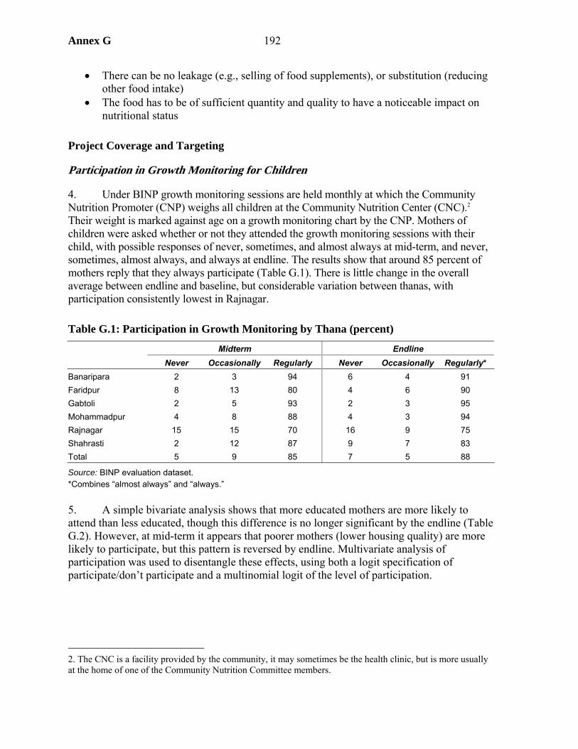
Annex G 192

• There can be no leakage (e.g., selling of food supplements), or substitution (reducing other food intake)

• The food has to be of sufficient quantity and quality to have a noticeable impact on nutritional status

Project Coverage and Targeting

Participation in Growth Monitoring for Children

4. Under BINP growth monitoring sessions are held monthly at which the Community Nutrition Promoter (CNP) weighs all children at the Community Nutrition Center (CNC).2 Their weight is marked against age on a growth monitoring chart by the CNP. Mothers of children were asked whether or not they attended the growth monitoring sessions with their child, with possible responses of never, sometimes, and almost always at mid-term, and never, sometimes, almost always, and always at endline. The results show that around 85 percent of mothers reply that they always participate (Table G.1). There is little change in the overall average between endline and baseline, but considerable variation between thanas, with participation consistently lowest in Rajnagar.

Table G.1: Participation in Growth Monitoring by Thana (percent)

Midterm Endline Never Occasionally Regularly Never Occasionally Regularly*

Banaripara 2 3 94 6 4 91 Faridpur 8 13 80 4 6 90 Gabtoli 2 5 93 2 3 95 Mohammadpur 4 8 88 4 3 94 Rajnagar 15 15 70 16 9 75 Shahrasti 2 12 87 9 7 83 Total 5 9 85 7 5 88

Source: BINP evaluation dataset. *Combines “almost always” and “always.” 5. A simple bivariate analysis shows that more educated mothers are more likely to attend than less educated, though this difference is no longer significant by the endline (Table G.2). However, at mid-term it appears that poorer mothers (lower housing quality) are more likely to participate, but this pattern is reversed by endline. Multivariate analysis of participation was used to disentangle these effects, using both a logit specification of participate/don’t participate and a multinomial logit of the level of participation.

2. The CNC is a facility provided by the community, it may sometimes be the health clinic, but is more usually at the home of one of the Community Nutrition Committee members.

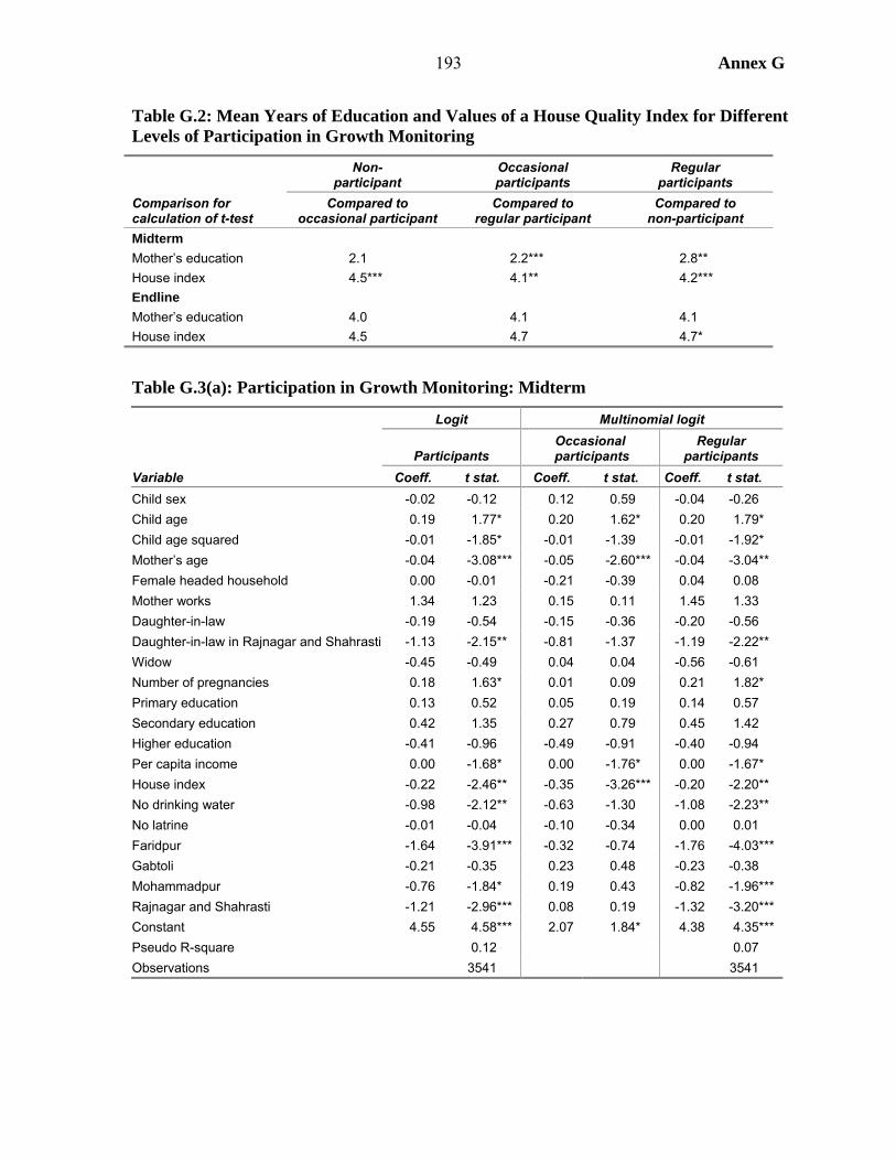
193 Annex G

Table G.2: Mean Years of Education and Values of a House Quality Index for Different Levels of Participation in Growth Monitoring

Non- participant

Occasional participants

Regular participants

Comparison for calculation of t-test

Compared to occasional participant

Compared to regular participant

Compared to non-participant

Midterm Mother’s education 2.1 2.2*** 2.8** House index 4.5*** 4.1** 4.2*** Endline Mother’s education 4.0 4.1 4.1 House index 4.5 4.7 4.7*

Table G.3(a): Participation in Growth Monitoring: Midterm

Logit Multinomial logit

Participants Occasional

participants Regular

participants Variable Coeff. t stat. Coeff. t stat. Coeff. t stat. Child sex -0.02 -0.12 0.12 0.59 -0.04 -0.26 Child age 0.19 1.77* 0.20 1.62* 0.20 1.79* Child age squared -0.01 -1.85* -0.01 -1.39 -0.01 -1.92* Mother’s age -0.04 -3.08*** -0.05 -2.60*** -0.04 -3.04** Female headed household 0.00 -0.01 -0.21 -0.39 0.04 0.08 Mother works 1.34 1.23 0.15 0.11 1.45 1.33 Daughter-in-law -0.19 -0.54 -0.15 -0.36 -0.20 -0.56 Daughter-in-law in Rajnagar and Shahrasti -1.13 -2.15** -0.81 -1.37 -1.19 -2.22** Widow -0.45 -0.49 0.04 0.04 -0.56 -0.61 Number of pregnancies 0.18 1.63* 0.01 0.09 0.21 1.82* Primary education 0.13 0.52 0.05 0.19 0.14 0.57 Secondary education 0.42 1.35 0.27 0.79 0.45 1.42 Higher education -0.41 -0.96 -0.49 -0.91 -0.40 -0.94 Per capita income 0.00 -1.68* 0.00 -1.76* 0.00 -1.67* House index -0.22 -2.46** -0.35 -3.26*** -0.20 -2.20** No drinking water -0.98 -2.12** -0.63 -1.30 -1.08 -2.23** No latrine -0.01 -0.04 -0.10 -0.34 0.00 0.01 Faridpur -1.64 -3.91*** -0.32 -0.74 -1.76 -4.03*** Gabtoli -0.21 -0.35 0.23 0.48 -0.23 -0.38 Mohammadpur -0.76 -1.84* 0.19 0.43 -0.82 -1.96*** Rajnagar and Shahrasti -1.21 -2.96*** 0.08 0.19 -1.32 -3.20*** Constant 4.55 4.58*** 2.07 1.84* 4.38 4.35*** Pseudo R-square 0.12 0.07 Observations 3541 3541

Annex G 194

6. The multivariate results, which are very similar for midterm and endline, show the following:

• There is no sex bias in participation. Participation has a non-linear relationship with the child’s age, with those aged 9-10 months most likely to attend.

• Both younger mothers and daughters-in-law are less likely to attend (daughter-in-law meaning here a woman living with her mother-in-law). The daughter-in-law dummy alone is significantly negative (results not shown), but is no longer so when an interactive term is included for the daughter-in-law dummy and the dummy for the two more conservative thanas, Rajnagar and Sharasti.3 The significant negative coefficient on this interactive term shows the effect of restrictions on female mobility in attending growth monitoring sessions, although they only have an effect in two of the six thanas. If the mother is employed outside the household, which is positively associated with women’s agency (Annex E), then she is more likely to participate. It is also the case that Hindu women are more likely to participate than Muslim.

• Qualitative analysis shows that remoteness (travel time) is also a constraint on participation. There is no direct measure of this variable in the dataset, but it is likely that type of water supply is a reasonable proxy for this variable (it is hard to imagine a direct effect of this variable), the results confirming that inferior forms of water supply (indicating remoteness) significantly reduce participation.4

• The results confirm that the most educated women are significantly less likely to participate. There is no income-bias in participation in the multivariate analysis, this result being roust to several different specifications (i.e., models which do not have other variables correlated to income, such as water and sanitation and parent’s education). However, at midterm the less poor are less likely to attend, based on both the housing quality index and the categorical income variable (based on the enumerator’s assessment). By contrast, at endline those with better housing are more likely to participate, but women in households with sizeable landholdings less likely to do so (reflecting a time constraint for such women, which is shown to be important when it comes to be putting knowledge into practice).

3. It is also more common for a woman to be living with their mother-in-law in these thanas, being so for 15 and 12 percent of respondents in Rajnagar and Sharasti respectively, compared to 9 percent on average.

4. The BINP dataset does not contain data on distances to health facilities. Using data of the Bangladesh Household Income and Expenditure Survey (HIES) of 2000-01, it was found that the time distance to the health provider sought for treatment was substantially longer for household not having access to drinking water (i.e., accessing water from rivers, ponds, rain, etc.). The difference was statistically significant using a t-test.

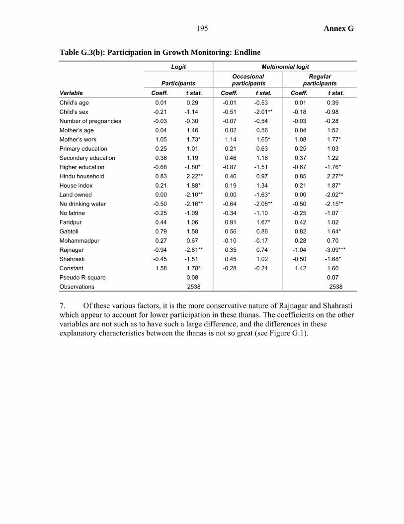
195 Annex G

Table G.3(b): Participation in Growth Monitoring: Endline

Logit Multinomial logit

Participants Occasional

participants Regular

participants Variable Coeff. t stat. Coeff. t stat. Coeff. t stat. Child’s age 0.01 0.29 -0.01 -0.53 0.01 0.39 Child’s sex -0.21 -1.14 -0.51 -2.01** -0.18 -0.98 Number of pregnancies -0.03 -0.30 -0.07 -0.54 -0.03 -0.28 Mother’s age 0.04 1.46 0.02 0.56 0.04 1.52 Mother’s work 1.05 1.73* 1.14 1.65* 1.08 1.77* Primary education 0.25 1.01 0.21 0.63 0.25 1.03 Secondary education 0.36 1.19 0.46 1.18 0.37 1.22 Higher education -0.68 -1.80* -0.87 -1.51 -0.67 -1.76* Hindu household 0.83 2.22** 0.46 0.97 0.85 2.27** House index 0.21 1.88* 0.19 1.34 0.21 1.87* Land owned 0.00 -2.10** 0.00 -1.63* 0.00 -2.02** No drinking water -0.50 -2.16** -0.64 -2.08** -0.50 -2.15** No latrine -0.25 -1.09 -0.34 -1.10 -0.25 -1.07 Faridpur 0.44 1.06 0.91 1.67* 0.42 1.02 Gabtoli 0.79 1.58 0.56 0.86 0.82 1.64* Mohammadpur 0.27 0.67 -0.10 -0.17 0.28 0.70 Rajnagar -0.94 -2.81** 0.35 0.74 -1.04 -3.09*** Shahrasti -0.45 -1.51 0.45 1.02 -0.50 -1.68* Constant 1.58 1.78* -0.28 -0.24 1.42 1.60 Pseudo R-square 0.08 0.07 Observations 2538 2538

7. Of these various factors, it is the more conservative nature of Rajnagar and Shahrasti which appear to account for lower participation in these thanas. The coefficients on the other variables are not such as to have such a large difference, and the differences in these explanatory characteristics between the thanas is not so great (see Figure G.1).

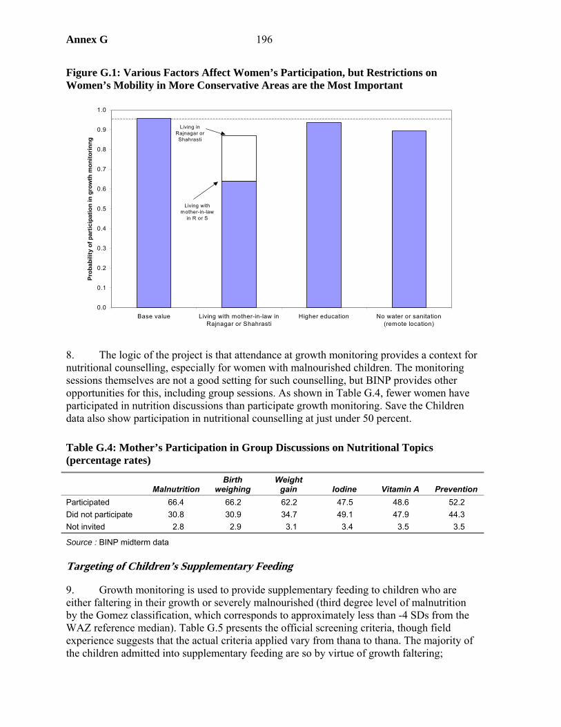
Annex G 196

Figure G.1: Various Factors Affect Women’s Participation, but Restrictions on Women’s Mobility in More Conservative Areas are the Most Important

8. The logic of the project is that attendance at growth monitoring provides a context for nutritional counselling, especially for women with malnourished children. The monitoring sessions themselves are not a good setting for such counselling, but BINP provides other opportunities for this, including group sessions. As shown in Table G.4, fewer women have participated in nutrition discussions than participate growth monitoring. Save the Children data also show participation in nutritional counselling at just under 50 percent.

Table G.4: Mother’s Participation in Group Discussions on Nutritional Topics (percentage rates)

Malnutrition Birth

weighing Weight

gain Iodine Vitamin A Prevention Participated 66.4 66.2 62.2 47.5 48.6 52.2 Did not participate 30.8 30.9 34.7 49.1 47.9 44.3 Not invited 2.8 2.9 3.1 3.4 3.5 3.5

Source : BINP midterm data Targeting of Children’s Supplementary Feeding

9. Growth monitoring is used to provide supplementary feeding to children who are either faltering in their growth or severely malnourished (third degree level of malnutrition by the Gomez classification, which corresponds to approximately less than -4 SDs from the WAZ reference median). Table G.5 presents the official screening criteria, though field experience suggests that the actual criteria applied vary from thana to thana. The majority of the children admitted into supplementary feeding are so by virtue of growth faltering;

0.0

0.1

0.2

0.3

0.4

0.5

0.6

0.7

0.8

0.9

1.0

Base value Living with mother-in-law inRajnagar or Shahrasti

Higher education No water or sanitation(remote location)

Prob

abili

ty o

f par

ticip

atio

n in

gro

wth

mon

itorin

ng

Living in Rajnagar or

Shahrasti

Living with mother-in-law

in R or S

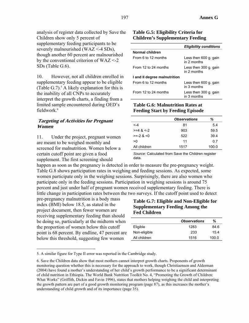
197 Annex G

analysis of register data collected by Save the Children show only 5 percent of supplementary feeding participants to be severely malnourished (WAZ <-4 SDs), though another 60 percent are malnourished by the conventional criterion of WAZ <-2 SDs (Table G.6).

10. However, not all children enrolled in supplementary feeding appear to be eligible (Table G.7).5 A likely explanation for this is the inability of all CNPs to accurately interpret the growth charts, a finding from a limited sample encountered during OED’s fieldwork.6

Targeting of Activities for Pregnant Women

11. Under the project, pregnant women are meant to be weighed monthly and screened for malnutrition. Women below a certain cutoff point are given a food supplement. The first screening should happen as soon as the pregnancy is detected in order to measure the pre-pregnancy weight. Table G.8 shows participation rates in weighing and feeding sessions. As expected, some women participate only in the weighing sessions. Surprisingly, there are also women who participate only in the feeding sessions. Participation in weighing sessions is around 75 percent and just under half of pregnant women received supplementary feeding. There is little change in participation rates between the two surveys. If the cutoff point used to detect pre-pregnancy malnutrition is a body mass index (BMI) below 18.5, as stated in the project document, then fewer women are receiving supplementary feeding than should be doing so, particularly at the midterm when the proportion of women below this cutoff point is 68 percent. By endline, 47 percent are below this threshold, suggesting few women

5. A similar figure for Type II error was reported in the Cambridge study.

6. Save the Children data show that most mothers cannot interpret growth charts. Proponents of growth monitoring question whether this is necessary for the approach to work, though Christiaensen and Alderman (2004) have found a mother’s understanding of her child’s growth performance to be a significant determinant of child nutrition in Ethiopia. The World Bank Nutrition Toolkit No. 4, “Promoting the Growth of Children: What Works” (Griffith, Dickin and Favin 1996), states that mothers helping weighing the child and interpreting the growth pattern are part of a good growth monitoring program (page 87), as this increases the mother’s understanding of child growth and of its importance (page 35).

Table G.5: Eligibility Criteria for Children’s Supplementary Feeding

Eligibility conditions Normal children From 6 to 12 months Less then 600 g. gain

in 2 months From 12 to 24 months Less then 300 g. gain

in 2 months I and II degree malnutrition From 6 to 12 months Less then 600 g. gain

in 3 months From 12 to 24 months Less then 300 g. gain

in 3 months

Table G.6: Malnutrition Rates at Feeding Start by Feeding Episode

Observations % <-4 81 5.4 >=4 & <-2 903 59.5 >=-2 & <0 522 39.4 >0 11 0.7 All children 1517 100.0

Source: Calculated from Save the Children register data.

Table G.7: Eligible and Non-Eligible for Supplementary Feeding Among the Fed Children

Observations % Eligible 1283 84.6 Non-eligible 233 15.4 All children 1516 100.0

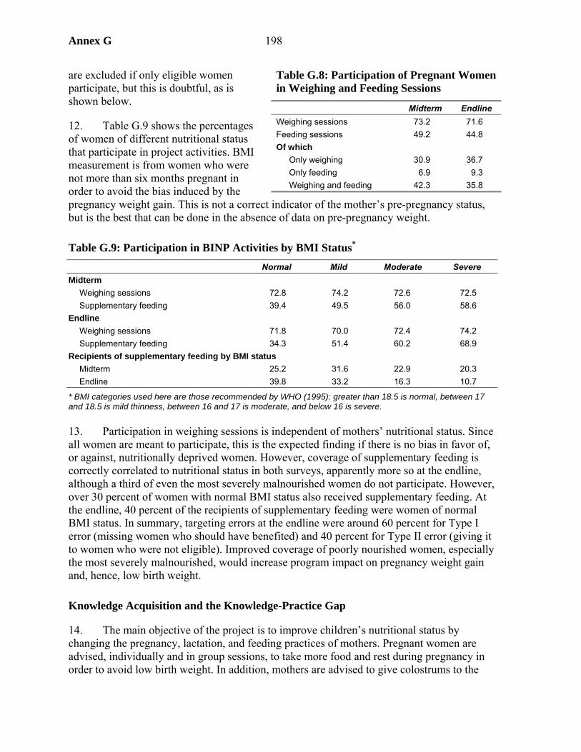
Annex G 198

are excluded if only eligible women participate, but this is doubtful, as is shown below.

12. Table G.9 shows the percentages of women of different nutritional status that participate in project activities. BMI measurement is from women who were not more than six months pregnant in order to avoid the bias induced by the pregnancy weight gain. This is not a correct indicator of the mother’s pre-pregnancy status, but is the best that can be done in the absence of data on pre-pregnancy weight.

Table G.9: Participation in BINP Activities by BMI Status*

Normal Mild Moderate Severe Midterm

Weighing sessions 72.8 74.2 72.6 72.5 Supplementary feeding 39.4 49.5 56.0 58.6

Endline Weighing sessions 71.8 70.0 72.4 74.2 Supplementary feeding 34.3 51.4 60.2 68.9

Recipients of supplementary feeding by BMI status Midterm 25.2 31.6 22.9 20.3 Endline 39.8 33.2 16.3 10.7

* BMI categories used here are those recommended by WHO (1995): greater than 18.5 is normal, between 17 and 18.5 is mild thinness, between 16 and 17 is moderate, and below 16 is severe. 13. Participation in weighing sessions is independent of mothers’ nutritional status. Since all women are meant to participate, this is the expected finding if there is no bias in favor of, or against, nutritionally deprived women. However, coverage of supplementary feeding is correctly correlated to nutritional status in both surveys, apparently more so at the endline, although a third of even the most severely malnourished women do not participate. However, over 30 percent of women with normal BMI status also received supplementary feeding. At the endline, 40 percent of the recipients of supplementary feeding were women of normal BMI status. In summary, targeting errors at the endline were around 60 percent for Type I error (missing women who should have benefited) and 40 percent for Type II error (giving it to women who were not eligible). Improved coverage of poorly nourished women, especially the most severely malnourished, would increase program impact on pregnancy weight gain and, hence, low birth weight.

Knowledge Acquisition and the Knowledge-Practice Gap

14. The main objective of the project is to improve children’s nutritional status by changing the pregnancy, lactation, and feeding practices of mothers. Pregnant women are advised, individually and in group sessions, to take more food and rest during pregnancy in order to avoid low birth weight. In addition, mothers are advised to give colostrums to the

Table G.8: Participation of Pregnant Women in Weighing and Feeding Sessions

Midterm Endline Weighing sessions 73.2 71.6 Feeding sessions 49.2 44.8 Of which

Only weighing 30.9 36.7 Only feeding 6.9 9.3 Weighing and feeding 42.3 35.8

199 Annex G

newborn and to practice exclusive breastfeeding of the infant up to the age of 5-6 months. For older children, advice is given on good nutrition. As outlined above there are several steps in the underlying theory behind this approach. This section investigates the third and fourth of these steps, that is, whether knowledge is acquired and if it is put into practice, failure to do so is labeled the knowledge-practice gap (KP gap).

Evidence from the Save the Children Data

15. The Save the Children study used three types of nutrition knowledge to calculate the KP gap. These are the knowledge on rest during pregnancy, colostrums, and exclusive breastfeeding reported in Table G.10.

16. Regarding knowledge, all the differences in knowledge between project and control areas are statistically significant, though these differences are not that great. There are differences in practice between project and control areas, but only one of them, rest during pregnancy, is statistically significant. Knowledge is generally high, being between 50 and 80 percent in both project and control areas. The KP gap is small in the case of colostrums, moderate in the case of rest, and extremely high in the case of exclusive breastfeeding. The project improves both knowledge and practice, but does not reduce the KP gap.

17. Regression analysis can be used to answer two questions: (1) What are the obstacles that prevent the knowledge being put into practice? and (2) Does the project help to reduce the KP gap in general, or for mothers with particular characteristics? The KP gap is modeled using a probit regression, where the dependent variable is one if there is a KP gap. The sample is composed of mothers who have the knowledge about the three nutritional practices described above. The estimation of this model can produce biased coefficients, because unobserved determinants of the knowledge can have effects on the practice as well. In order to avoid this bias a two-step Heckman approach is adopted, first estimating a selection equation explaining the knowledge among mothers, and then a gap equation for mothers who have the knowledge. The results are in Table G.11.

Table G.10: Nutrition Knowledge of Pregnant and Lactating Mothers (Save the Children data)

Project Control t stat. Rest during pregnancy

Knowledge 77.1 69.4 4.00*** Practice 58.4 52.3 3.56*** KP gap 30.7 34.7 -2.15**

Colostrum Knowledge 75.4 71.9 4.33*** Practice 62.7 51.5 1.53 KP gap 18.3 21.1 -1.30

Breastfeeding Knowledge 77.6 68.7 5.06*** Practice 3.6 4.9 -1.16 KP gap 95.7 94.2 1.08

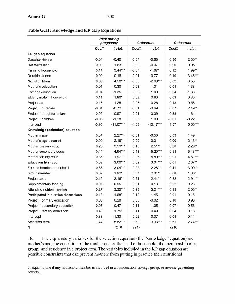
Annex G 200

Table G.11: Knowledge and KP Gap Equations

Rest during pregnancy Colostrum Colostrum

Coeff. t stat. Coeff. t stat. Coeff. t stat. KP gap equation Daughter-in-law -0.04 -0.40 -0.07 -0.68 0.30 2.30** H/h owns land 0.00 1.63* 0.00 -0.07 0.00 0.95 Farming household 0.14 3.44*** -0.07 -1.67* 0.12 1.99** Durables index 0.00 -0.16 -0.01 -0.77 -0.10 -3.46*** No. of children 0.09 4.58*** -0.06 -2.69*** 0.02 0.53 Mother’s education -0.01 -0.30 0.03 1.01 0.04 1.38 Father’s education -0.04 -1.35 0.03 1.00 -0.04 -1.36 Elderly male in household 0.11 1.90* 0.03 0.60 0.03 0.35 Project area 0.13 1.25 0.03 0.26 -0.13 -0.58 Project * durables -0.01 -0.72 -0.01 -0.69 0.07 2.49** Project * daughter-in-law -0.06 -0.57 -0.01 -0.09 -0.28 -1.81* Project * children -0.03 -1.28 0.03 1.00 -0.01 -0.22 Intercept -0.95 -11.07*** -1.08 -10.17*** 1.57 5.66*** Knowledge (selection) equation Mother’s age 0.04 2.27** -0.01 -0.50 0.03 1.49 Mother’s age squared 0.00 -2.18** 0.00 0.01 0.00 -2.13** Mother primary educ. 0.26 3.59*** 0.18 2.51** 0.20 2.29** Mother secondary educ. 0.44 4.94*** 0.43 5.20*** 0.54 5.43*** Mother tertiary educ. 0.36 1.97** 0.98 5.80*** 0.91 4.61*** Education h/h head 0.02 3.00*** 0.02 3.04*** 0.01 2.07** Female headed household 0.33 3.04*** 0.22 2.28** 0.41 3.90*** Group member 0.07 1.92* 0.07 2.04** 0.08 1.86* Project area 0.16 2.16** 0.21 2.44** 0.22 2.94*** Supplementary feeding -0.07 -0.95 0.01 0.13 -0.02 -0.26 Attending nutrion meeting 0.27 3.35*** 0.23 3.24*** 0.19 2.08** Participated in nutrition discussions 0.13 1.68* 0.12 1.45 0.01 0.16 Project * primary education 0.03 0.28 0.00 -0.02 0.10 0.93 Project * secondary education 0.05 0.47 0.11 1.05 0.07 0.58 Project * tertiary education 0.40 1.75* 0.11 0.49 0.04 0.18 Intercept -0.38 -1.33 0.02 0.07 -0.04 -0.14 Selection term 1.44 5.82*** 1.89 3.33*** 0.61 2.74*** N 7216 7217 7216

18. The explanatory variables for the selection equation (the “knowledge” equation) are mother’s age, the education of the mother and of the head of household, the membership of a group,7 and residence in a project area. The variables included in the KP gap equation are possible constraints that can prevent mothers from putting in practice their nutritional

7. Equal to one if any household member is involved in an association, savings group, or income-generating activity.

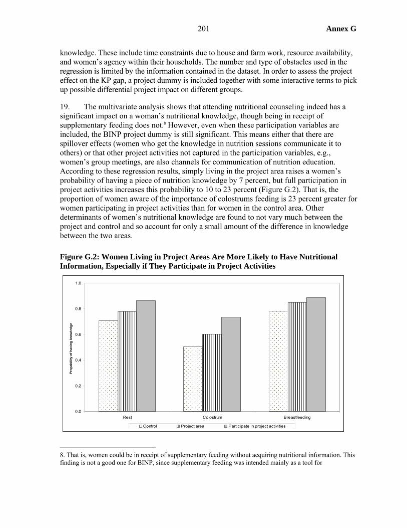
201 Annex G

knowledge. These include time constraints due to house and farm work, resource availability, and women’s agency within their households. The number and type of obstacles used in the regression is limited by the information contained in the dataset. In order to assess the project effect on the KP gap, a project dummy is included together with some interactive terms to pick up possible differential project impact on different groups.

19. The multivariate analysis shows that attending nutritional counseling indeed has a significant impact on a woman’s nutritional knowledge, though being in receipt of supplementary feeding does not.8 However, even when these participation variables are included, the BINP project dummy is still significant. This means either that there are spillover effects (women who get the knowledge in nutrition sessions communicate it to others) or that other project activities not captured in the participation variables, e.g., women’s group meetings, are also channels for communication of nutrition education. According to these regression results, simply living in the project area raises a women’s probability of having a piece of nutrition knowledge by 7 percent, but full participation in project activities increases this probability to 10 to 23 percent (Figure G.2). That is, the proportion of women aware of the importance of colostrums feeding is 23 percent greater for women participating in project activities than for women in the control area. Other determinants of women’s nutritional knowledge are found to not vary much between the project and control and so account for only a small amount of the difference in knowledge between the two areas.

Figure G.2: Women Living in Project Areas Are More Likely to Have Nutritional Information, Especially if They Participate in Project Activities

8. That is, women could be in receipt of supplementary feeding without acquiring nutritional information. This finding is not a good one for BINP, since supplementary feeding was intended mainly as a tool for

0.0

0.2

0.4

0.6

0.8

1.0

Rest Colostrum Breastfeeding

Pro

pabi

lity

of h

avin

g kn

owle

dge

Control Project area Participate in project activities

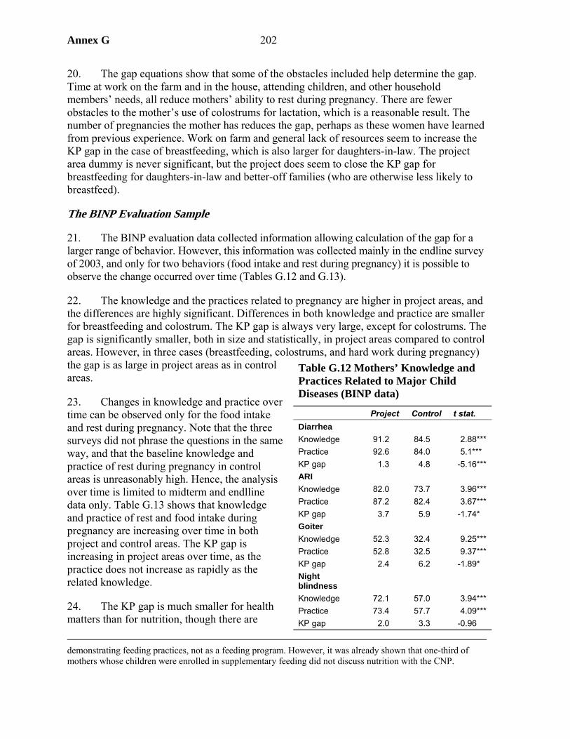
Annex G 202

20. The gap equations show that some of the obstacles included help determine the gap. Time at work on the farm and in the house, attending children, and other household members’ needs, all reduce mothers’ ability to rest during pregnancy. There are fewer obstacles to the mother’s use of colostrums for lactation, which is a reasonable result. The number of pregnancies the mother has reduces the gap, perhaps as these women have learned from previous experience. Work on farm and general lack of resources seem to increase the KP gap in the case of breastfeeding, which is also larger for daughters-in-law. The project area dummy is never significant, but the project does seem to close the KP gap for breastfeeding for daughters-in-law and better-off families (who are otherwise less likely to breastfeed).

The BINP Evaluation Sample

21. The BINP evaluation data collected information allowing calculation of the gap for a larger range of behavior. However, this information was collected mainly in the endline survey of 2003, and only for two behaviors (food intake and rest during pregnancy) it is possible to observe the change occurred over time (Tables G.12 and G.13).

22. The knowledge and the practices related to pregnancy are higher in project areas, and the differences are highly significant. Differences in both knowledge and practice are smaller for breastfeeding and colostrum. The KP gap is always very large, except for colostrums. The gap is significantly smaller, both in size and statistically, in project areas compared to control areas. However, in three cases (breastfeeding, colostrums, and hard work during pregnancy) the gap is as large in project areas as in control areas.

23. Changes in knowledge and practice over time can be observed only for the food intake and rest during pregnancy. Note that the three surveys did not phrase the questions in the same way, and that the baseline knowledge and practice of rest during pregnancy in control areas is unreasonably high. Hence, the analysis over time is limited to midterm and endlline data only. Table G.13 shows that knowledge and practice of rest and food intake during pregnancy are increasing over time in both project and control areas. The KP gap is increasing in project areas over time, as the practice does not increase as rapidly as the related knowledge.

24. The KP gap is much smaller for health matters than for nutrition, though there are

demonstrating feeding practices, not as a feeding program. However, it was already shown that one-third of mothers whose children were enrolled in supplementary feeding did not discuss nutrition with the CNP.

Table G.12 Mothers’ Knowledge and Practices Related to Major Child Diseases (BINP data)

Project Control t stat. Diarrhea Knowledge 91.2 84.5 2.88*** Practice 92.6 84.0 5.1*** KP gap 1.3 4.8 -5.16*** ARI Knowledge 82.0 73.7 3.96*** Practice 87.2 82.4 3.67*** KP gap 3.7 5.9 -1.74* Goiter Knowledge 52.3 32.4 9.25*** Practice 52.8 32.5 9.37*** KP gap 2.4 6.2 -1.89* Night blindness

Knowledge 72.1 57.0 3.94*** Practice 73.4 57.7 4.09*** KP gap 2.0 3.3 -0.96

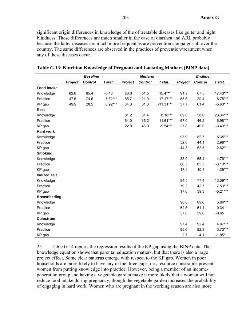
203 Annex G

significant origin differences in knowledge of the of treatable diseases like goiter and night blindness. These differences are much smaller in the case of diarrhea and ARI, probably because the latter diseases are much more frequent as are prevention campaigns all over the country. The same differences are observed in the practices of prevention/treatment when any of these diseases occur.

Table G.13: Nutrition Knowledge of Pregnant and Lactating Mothers (BINP data)

Baseline Midterm Endline Project Control t stat. Project Control t stat. Project Control t stat. Food intake Knowledge 62.8 65.4 -0.48 83.6 51.5 15.4*** 91.9 67.5 17.43*** Practice 47.5 74.6 -7.52*** 55.7 21.9 17.17*** 58.6 29.4 8.75*** KP gap 49.9 20.5 6.92*** 34.3 61.3 -11.31*** 37.7 61.4 -5.63*** Rest Knowledge 81.2 61.4 8.18*** 89.0 58.0 23.36*** Practice 64.0 35.2 11.61*** 67.0 46.2 6.98*** KP gap 22.8 46.9 -9.54*** 27.8 40.0 -3.49*** Hard work Knowledge 93.9 82.7 5.35*** Practice 52.6 44.1 2.98*** KP gap 44.8 52.5 -2.62** Smoking Knowledge 88.0 65.4 4.76*** Practice 80.5 85.5 -3.13*** KP gap 17.9 10.4 4.35*** Iodized salt Knowledge 94.5 77.4 13.09*** Practice 79.2 42.7 7.53*** KP gap 17.6 39.3 -5.21*** Breastfeeding Knowledge 96.6 89.6 5.86*** Practice 62.5 61.1 0.34 KP gap 37.0 39.6 -0.65 Colostrum Knowledge 97.4 92.4 4.87*** Practice 95.6 92.3 3.73*** KP gap 2.7 4.1 -1.85*

25. Table G.14 reports the regression results of the KP gap using the BINP data. The knowledge equation shows that parental education matters, but that there is also a large project effect. Some clear patterns emerge with respect to the KP gap. Women in poor households are more likely to have any of the three gaps, i.e., resource constraints prevent women from putting knowledge into practice. However, being a member of an income-generation group and having a vegetable garden make it more likely that a woman will not reduce food intake during pregnancy, though the vegetable garden increases the probability of engaging in hard work. Women who are pregnant in the working season are also more

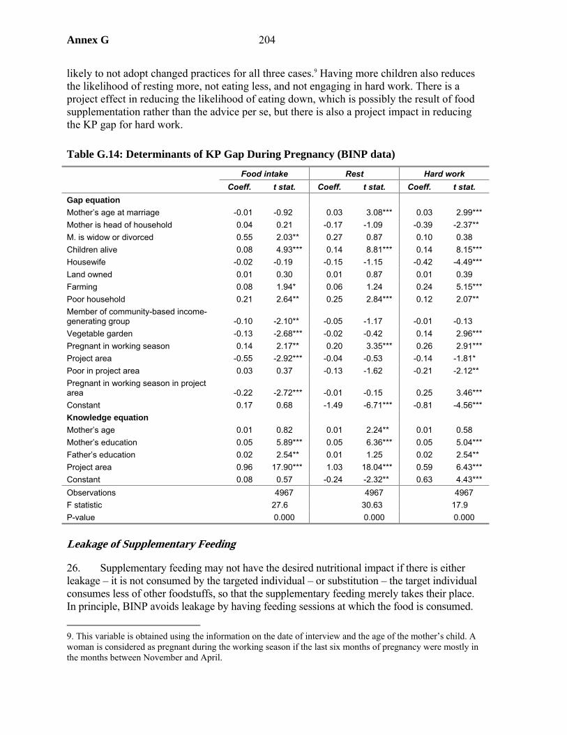
Annex G 204

likely to not adopt changed practices for all three cases.9 Having more children also reduces the likelihood of resting more, not eating less, and not engaging in hard work. There is a project effect in reducing the likelihood of eating down, which is possibly the result of food supplementation rather than the advice per se, but there is also a project impact in reducing the KP gap for hard work.

Table G.14: Determinants of KP Gap During Pregnancy (BINP data)

Food intake Rest Hard work Coeff. t stat. Coeff. t stat. Coeff. t stat.

Gap equation Mother’s age at marriage -0.01 -0.92 0.03 3.08*** 0.03 2.99*** Mother is head of household 0.04 0.21 -0.17 -1.09 -0.39 -2.37** M. is widow or divorced 0.55 2.03** 0.27 0.87 0.10 0.38 Children alive 0.08 4.93*** 0.14 8.81*** 0.14 8.15*** Housewife -0.02 -0.19 -0.15 -1.15 -0.42 -4.49*** Land owned 0.01 0.30 0.01 0.87 0.01 0.39 Farming 0.08 1.94* 0.06 1.24 0.24 5.15*** Poor household 0.21 2.64** 0.25 2.84*** 0.12 2.07** Member of community-based income-generating group -0.10 -2.10** -0.05 -1.17 -0.01 -0.13 Vegetable garden -0.13 -2.68*** -0.02 -0.42 0.14 2.96*** Pregnant in working season 0.14 2.17** 0.20 3.35*** 0.26 2.91*** Project area -0.55 -2.92*** -0.04 -0.53 -0.14 -1.81* Poor in project area 0.03 0.37 -0.13 -1.62 -0.21 -2.12** Pregnant in working season in project area -0.22 -2.72*** -0.01 -0.15 0.25 3.46*** Constant 0.17 0.68 -1.49 -6.71*** -0.81 -4.56*** Knowledge equation Mother’s age 0.01 0.82 0.01 2.24** 0.01 0.58 Mother’s education 0.05 5.89*** 0.05 6.36*** 0.05 5.04*** Father’s education 0.02 2.54** 0.01 1.25 0.02 2.54** Project area 0.96 17.90*** 1.03 18.04*** 0.59 6.43*** Constant 0.08 0.57 -0.24 -2.32** 0.63 4.43*** Observations 4967 4967 4967 F statistic 27.6 30.63 17.9 P-value 0.000 0.000 0.000

Leakage of Supplementary Feeding

26. Supplementary feeding may not have the desired nutritional impact if there is either leakage – it is not consumed by the targeted individual – or substitution – the target individual consumes less of other foodstuffs, so that the supplementary feeding merely takes their place. In principle, BINP avoids leakage by having feeding sessions at which the food is consumed. 9. This variable is obtained using the information on the date of interview and the age of the mother’s child. A woman is considered as pregnant during the working season if the last six months of pregnancy were mostly in the months between November and April.

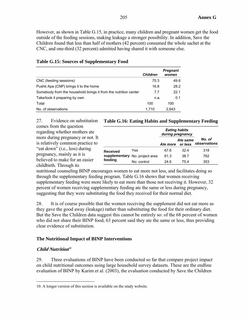
205 Annex G

However, as shown in Table G.15, in practice, many children and pregnant women get the food outside of the feeding sessions, making leakage a stronger possibility. In addition, Save the Children found that less than half of mothers (42 percent) consumed the whole sachet at the CNC, and one-third (32 percent) admitted having shared it with someone else.

Table G.15: Sources of Supplementary Food

Children Pregnant women

CNC (feeding sessions) 75.3 49.6 Pushti Apa (CNP) brings it to the home 16.8 28.2 Somebody from the household brings it from the nutrition center 7.7 22.1 Take/took it preparing by own n.a. 0.1 Total 100 100 No. of observations 1,710 2,643

27. Evidence on substitution comes from the question regarding whether mothers ate more during pregnancy or not. It is relatively common practice to “eat down” (i.e., less) during pregnancy, mainly as it is believed to make for an easier childbirth. Through its nutritional counseling BINP encourages women to eat more not less, and facilitates doing so through the supplementary feeding program. Table G.16 shows that women receiving supplementary feeding were more likely to eat more than those not receiving it. However, 32 percent of women receiving supplementary feeding ate the same or less during pregnancy, suggesting that they were substituting the food they received for their normal diet.

28. It is of course possible that the women receiving the supplement did not eat more as they gave the good away (leakage) rather than substituting the food for their ordinary diet. But the Save the Children data suggest this cannot be entirely so: of the 68 percent of women who did not share their BINP food, 63 percent said they ate the same or less, thus providing clear evidence of substitution.

The Nutritional Impact of BINP Interventions

Child Nutrition10

29. Three evaluations of BINP have been conducted so far that compare project impact on child nutritional outcomes using large household survey datasets. These are the endline evaluation of BINP by Karim et al. (2003), the evaluation conducted by Save the Children

10. A longer version of this section is available on the study website.

Table G.16: Eating Habits and Supplementary Feeding

Eating habits

during pregnancy

Ate more Ate same

or less No. of

observations

Yes 67.6 32.4 318 No: project area 61.3 38.7 762

Received supplementary feeding No: control 24.6 75.4 353

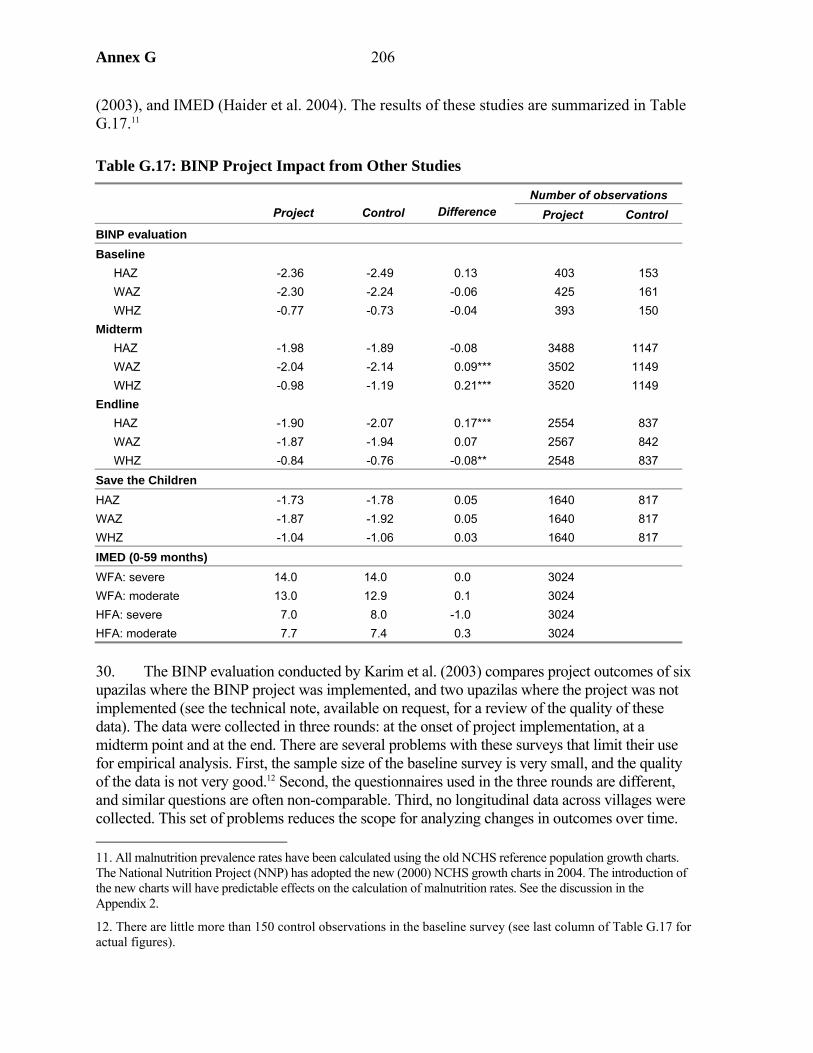
Annex G 206

(2003), and IMED (Haider et al. 2004). The results of these studies are summarized in Table G.17.11

Table G.17: BINP Project Impact from Other Studies

Number of observations

Project

Control Difference Project Control

BINP evaluation Baseline

HAZ -2.36 -2.49 0.13 403 153 WAZ -2.30 -2.24 -0.06 425 161 WHZ -0.77 -0.73 -0.04 393 150

Midterm HAZ -1.98 -1.89 -0.08 3488 1147 WAZ -2.04 -2.14 0.09*** 3502 1149 WHZ -0.98 -1.19 0.21*** 3520 1149

Endline HAZ -1.90 -2.07 0.17*** 2554 837 WAZ -1.87 -1.94 0.07 2567 842 WHZ -0.84 -0.76 -0.08** 2548 837

Save the Children HAZ -1.73 -1.78 0.05 1640 817 WAZ -1.87 -1.92 0.05 1640 817 WHZ -1.04 -1.06 0.03 1640 817 IMED (0-59 months) WFA: severe 14.0 14.0 0.0 3024 WFA: moderate 13.0 12.9 0.1 3024 HFA: severe 7.0 8.0 -1.0 3024 HFA: moderate 7.7 7.4 0.3 3024

30. The BINP evaluation conducted by Karim et al. (2003) compares project outcomes of six upazilas where the BINP project was implemented, and two upazilas where the project was not implemented (see the technical note, available on request, for a review of the quality of these data). The data were collected in three rounds: at the onset of project implementation, at a midterm point and at the end. There are several problems with these surveys that limit their use for empirical analysis. First, the sample size of the baseline survey is very small, and the quality of the data is not very good.12 Second, the questionnaires used in the three rounds are different, and similar questions are often non-comparable. Third, no longitudinal data across villages were collected. This set of problems reduces the scope for analyzing changes in outcomes over time. 11. All malnutrition prevalence rates have been calculated using the old NCHS reference population growth charts. The National Nutrition Project (NNP) has adopted the new (2000) NCHS growth charts in 2004. The introduction of the new charts will have predictable effects on the calculation of malnutrition rates. See the discussion in the Appendix 2.

12. There are little more than 150 control observations in the baseline survey (see last column of Table G.17 for actual figures).

207 Annex G

There are also problems that limit the use of the cross-sectional aspect of these data. First, anthropometric measurements of children were taken at different times of the year. Given the high seasonality of child malnutrition in Bangladesh, this is a potential source of bias. Second, while the sample of project thanas is representative of all Bangladeshi divisions, the sample of control thanas is not. If there are substantial differences in nutrition determinants between regions, comparisons of outcomes can be biased. Third, some of the selected control thanas may have benefited of nutrition projects of other NGOs. In one of the thanas, BRAC (the implementing NGO of the first phase BINP thanas) operated nutrition activities in the same period as the BINP was implemented (Karim et al. 2003). There is a risk that the control thanas do not represent a sample of household “without the project.”13 Finally, the control samples are particularly small, especially at the baseline.

31. Save the Children collected data between March and May 2002 in three of the first-phase BINP thanas, and in three control thanas. According to Save the Children, these control thanas do not have serious problems with “contamination,” and lack of regional representativeness, as the BINP control group. However, the control sample is very small, and there is the possibility of seasonal bias, which cannot be assessed since dates of anthropometric measurements are not reported in the dataset. Finally, the IMED study collected data from 12 project upazillas from all three phases of BINP 12 controls selected from neighboring upazillas. Both studies have to rely on single difference estimates of project impact, and so depend on strong assumptions regarding the quality of the control.

32. According to the BINP evaluation data there was no difference between project and control areas for the mean of any of the three z-scores at the baseline. There is a significant project effect on weight for age at the midterm. Height for age, however, remained unchanged, resulting in a very large effect on weight for height. At the endline, the data show a significant project effect on height for age. However, it is not clear how this could happen, since the project did not succeed in improving weight for age for the same children. The endline difference in weight for age is a combination of the difference in weight for age and height for age. Since heights are increasing and weights are stable, weight for height decreases.

33. The Save the Children data show no significant differences between the project and control. The IMED data show not much difference either, though there is a slight difference in severe stunting, partly offset by higher moderate stunting in project areas.14 This finding is consistent with the BINP evaluation, which also suggested that some children were moved from severely to moderately stunted.

34. In summary, these studies find either no project effect, or where there is one, it appears relatively small.15 There are two problems connected to the estimation of project effects presented above: (1) the possible poor quality of the control, and (2) the estimated effects are 13. The fact that knowledge has not risen in control thanas suggest that contamination is not a serious problem.

14. The text of the IMED report claims a larger impact if considering only the weight for height proportion of children aged 0-23 months.

15. One possibility, which cannot be explored with the data to hand, is that improved nutrition was expended in extra physical activity rather than weight gain.

Annex G 208

average population effects that conflate two issues, project participation and effect on those who participate. This study improves on these estimates of project effects by using national data to create a comparison group, and by separating participation (analyzed above) from impact on participants.

35. The comparison group for this study is constructed based on the characteristics of the child and of its household of origin using data from Helen Keller’s Nutritional Surveillance Survey (Box G.1), using the method of propensity score matching (see Appendix 3). Project effects are estimated only for the BINP evaluation samples of midterm and endline children. For several reasons a similar analysis cannot be applied to the children sampled by the Save the Children survey.16

36. NSP data were used only from the rounds that correspond to the time of collection of the midterm and endline BINP surveys. This restriction is necessary given the high sensitivity of nutritional indicators to seasonal variations in Bangladesh. The rounds used are therefore the October/November and December/January rounds for the midterm evaluation, and the December/January and the February/March rounds for the endline evaluation. These data are complemented with the data from the comparison sites that were collected for the BINP evaluation. There are 7,091 control observation against 3,000 project observations at the midterm, and 6,247 control observations against 2,269 project observations at the endline.17

37. To create a match it is necessary to estimate the propensity to participate using a model which: (1) avoids explanatory variables that are influenced by the project, (2) includes of all possible observable determinants of participation, and in particular those that are influencing both outcomes and participation. It was shown above that various factors

16. It is not possible to discern from the Save the Children questionnaire the children who participated in GMP from those who did not. In addition, there is little information that can be used to identify participants in a model of participation. Finally, the absence of data on the date of the interview is also a concern, because of the sensitivity of nutritional indicators to seasonal effects.

17. After selecting NSP data of the same months in which the BINP data were collected, some discrepancies in the temporal distribution of the observations BINP and NSP data still remains. In order to correct this source of seasonal variation in nutritional indicators, the data were seasonally adjusted.

Box G.1: The Helen Keller International Nutritional Surveillance Project (NSP) In 1990 the NSP started collecting data on health and nutrition of mothers and children of Bangladesh. Data are collected bi-monthly in “rounds” corresponding to six Bangladeshi seasons. At each round, the data collection takes place in six or seven weeks, from approximately 10,000 rural households. The household is interviewed only if it contains at least one physically able child under five years of age (aged between 6 and 59 months prior to 2000), and if the mother is available. Starting from February 1998, the data are nationally representative. Four thanas were randomly selected from each administrative division, which makes a total of 24 thanas. At each survey round, 15 mauzas (10 prior to 2000) are randomly selected with probability proportional to size from each thana. One village is randomly selected from each mauza (administrative unit within a thana), and 25 households are systematically sampled from each village. Thus, while the 24 thanas that were selected in 1998 are always the same, the villages and the households interviewed differ at every round. The data constitute a series of repeated cross-sections. The dataset contains 49 variables, including location variables, household and child characteristics and anthropometric measurements.

209 Annex G

influence participation. Model specification is more constrained here, since only variables also available in NSP can be included in the model. Table G.18 lists the variables used in the specification of the selection model including their definition in the two datasets used (the BINP evaluation and the NSP data). The second column describes how the variables from the two datasets compare. The third column explains the inclusion of the variable in the model when the reason is not obvious. The results from these equations were used to estimate the propensity scores for the purposes of matching.18

Table G.18: Definition of the Variables Used in the Model Variable Specification Notes Child age Age is in completed months. Child sex Gender of the child is 1 for female. Child is breastfed Whether the child is breastfed at the time of the interview. Children over 6 months only, and

therefore is independent of the project, which recommends exclusive breastfeeding for children under 6 months.

Season of birth of the child

The season in which the child was born obtained using date of birth and date of interview.

This is a weak correlate of low birth weight, which in turn is a determinant of future nutritional status.

Mother’s age Age in completed years. Female-headed household

The mother is head of the household.

Widow or divorced Whether the marital status of the mother is widow or divorced. Mother’s height Mother’s height measured in centimeters. This predict child’s height. Largely

missing before 1998. Mother is pregnant Whether the mother is pregnant at the time of the interview. Pregnant mothers are specifically

targeted by the project. Household size This is the number of people who live together and take food from the

same pot (NSP). The definition used by BINP is not known.

Number of children under five

Number of children under five. Prior 2000 only the number of children aged between 6 and 59 months was recorded.

Occupation of head of household

NSP: Occupation of the person that provides the majority of household income. BINP: occupation of the head of household. BINP midterm and endline surveys used different categories

We assume that the main earner and head of household are the same

Mother’s education Four levels of education are defined: illiterate, primary (including uncompleted), secondary (including uncompleted) and higher. The variable is originally the number of completed years of schooling in both NSP and BINP.

Father education Same as for the mother. House This is the area size of the house where household lives. It is

measured in square feet based on measurements of width and length.

This is a correlate of wealth.

Land This is the land owned by the household in decimals. Land that is rented, sharecropped, and homestead garden are not included.

Landlessness Household with no land. Without well Household without a tubewell from which obtaining drinking water (so

use pond or river water or rain water).

Without latrine Households without an open or closed latrine. These households dispose of excreta in rivers or in the bush.

18. It is questionable whether the equation can be estimated using the HKI data since households outside the project area could not participate even if they wanted to. An alternative procedure is to estimate the participation equation using only the project sample and then apply those coefficients to the NSP data to calculate the scores. This approach was also used, with the final results not being much different from those shown here.

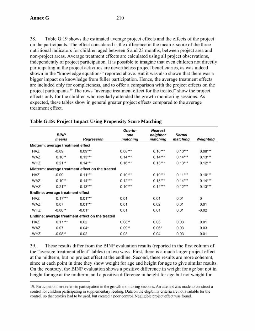
Annex G 210

38. Table G.19 shows the estimated average project effects and the effects of the project on the participants. The effect considered is the difference in the mean z-score of the three nutritional indicators for children aged between 6 and 23 months, between project area and non-project areas. Average treatment effects are calculated using all project observations, independently of project participation. It is possible to imagine that even children not directly participating in the project activities are nevertheless project beneficiaries, as was indeed shown in the “knowledge equations” reported above. But it was also shown that there was a bigger impact on knowledge from fuller participation. Hence, the average treatment effects are included only for completeness, and to offer a comparison with the project effects on the project participants.19 The rows “average treatment effect for the treated” show the project effects only for the children who regularly attended the growth monitoring sessions. As expected, these tables show in general greater project effects compared to the average treatment effect.

Table G.19: Project Impact Using Propensity Score Matching

BINP

means Regression

One-to- one

matching

Nearest neighbormatching

Kernel matching Weighting

Midterm: average treatment effect HAZ -0.09 0.09*** 0.08*** 0.10*** 0.10*** 0.08*** WAZ 0.10** 0.13*** 0.14*** 0.14*** 0.14*** 0.13*** WHZ 0.21** 0.14*** 0.16*** 0.13*** 0.13*** 0.12*** Midterm: average treatment effect on the treated HAZ -0.09 0.11*** 0.10*** 0.10*** 0.11*** 0.10*** WAZ 0.10** 0.14*** 0.12*** 0.13*** 0.14*** 0.14*** WHZ 0.21** 0.13*** 0.10*** 0.12*** 0.12*** 0.13*** Endline: average treatment effect HAZ 0.17*** 0.01*** 0.01 0.01 0.01 0 WAZ 0.07 0.01*** 0.01 0.02 0.01 0.01 WHZ -0.08** -0.01* 0.01 0.01 0.01 -0.02 Endline: average treatment effect on the treated HAZ 0.17*** 0.02 0.08** 0.03 0.03 0.01 WAZ 0.07 0.04* 0.09** 0.06* 0.03 0.03 WHZ -0.08** 0.02 0.03 0.04 0.03 0.01

39. These results differ from the BINP evaluation results (reported in the first column of the “average treatment effect” tables) in two ways. First, there is a much larger project effect at the midterm, but no project effect at the endline. Second, these results are more coherent, since at each point in time they show weight for age and height for age to give similar results. On the contrary, the BINP evaluation shows a positive difference in weight for age but not in height for age at the midterm, and a positive difference in height for age but not weight for 19. Participation here refers to participation in the growth monitoring sessions. An attempt was made to construct a control for children participating in supplementary feeding. Data on the eligibility criteria are not available for the control, so that proxies had to be used, but created a poor control. Negligible project effect was found.

211 Annex G

age at the endline, which is not clear why, given that height for age scores are the cumulated results of weight for age scores. The results also differ from the Save the Children evaluation in that there is a project effect on weight for age at the endline, though this effect is very weak.

40. These results can be summarized as follows:

• There is evidence of a project effect for all nutritional indicators at the midterm, and for weight-for-age at the endline.

• The size of the effect is small (negligible in the case of the endline data), a reduction of 0.1 z-scores is equivalent to a 3-4 percent reduction of malnutrition rates.

• There is evidence that the project performance was worse at the endline with respect to the midterm.

41. Table G.20 presents the estimated projects effects corresponding to different levels of project participation.20 There is evidence of a project effect only for children who participated regularly in the project.

42. Tables G.20 and G.21 show project impact according to nutritional status.21 Children measuring between -3 and -2 z-scores are normally considered malnourished. Children scoring less than -3 are normally considered severely malnourished. The category of the severely malnourished children is split into those who score between -3 and -4, and those who score less than -4. A z-score of -4 is approximately the cutoff point used to define the third-degree level of malnutrition in the Gomez classification. This category is interesting because children scoring less than -4 have much higher mortality risk than other children, and because the project is targeting children of third degree of Gomez malnutrition for food supplementation. Figure G.3 provides a visual representation of the same distribution of z-scores. Z-scores in healthy populations have a distribution that is very close to the normal distribution. The percentage of children below -2 z-scores is normally 2.3. The vertical lines in the charts help to assess the difference in malnutrition rates between project and non-project areas.

43. The shapes of the midterm and endline distributions are very similar, although project effects at the endline are much smaller. For all nutritional indicators the project has the effect of shifting the distribution to the right. In particular, it reduces the number of malnourished children between -3 and -2 z-scores, and increases the number of normal children. In

20. Project effects are estimated by running ordered logit models of participation, where the dependent variable takes three values: 0 for non-participation, 1 for irregular participation, and 2 for continuous participation. The predicted probability are used to weight the observations. Outcomes of children whose mother made the choice 2 are weighted by the inverse of the predicted probability of that choice. The project effect is calculated taking the difference between this value and the mean outcomes of the children who did not participate.

21. Tables G.20 and G.21, and the charts in Figure G.3 are based on matched observations of BINP evaluation sample and NSP data, performed with the one-to-one matching method.

Table G.20: Project Effect by Level of Participation

Midterm Endline Irregular Regular Irregular Regular

HAZ -0.06 0.08*** 0.03 0.01 WAZ 0.05 0.13*** 0.02 0.03 WHZ 0.07 0.13*** -0.02 0.02

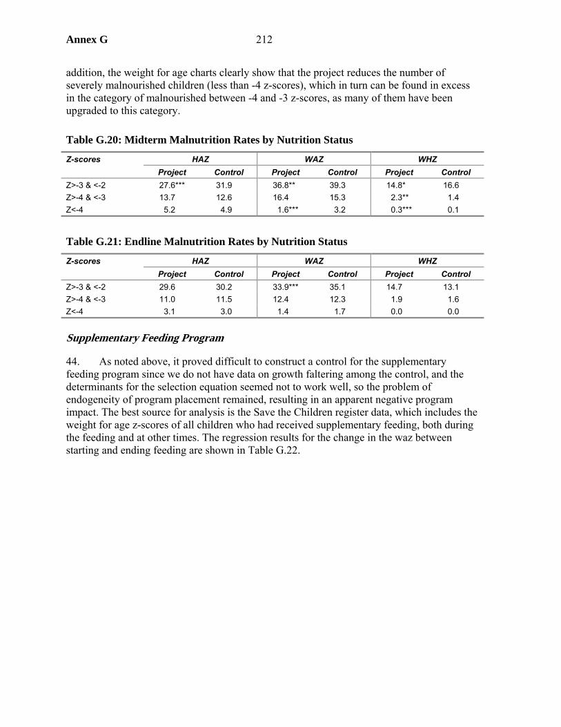
Annex G 212

addition, the weight for age charts clearly show that the project reduces the number of severely malnourished children (less than -4 z-scores), which in turn can be found in excess in the category of malnourished between -4 and -3 z-scores, as many of them have been upgraded to this category.

Table G.20: Midterm Malnutrition Rates by Nutrition Status

Z-scores HAZ WAZ WHZ Project Control Project Control Project Control Z>-3 & <-2 27.6*** 31.9 36.8** 39.3 14.8* 16.6 Z>-4 & <-3 13.7 12.6 16.4 15.3 2.3** 1.4 Z<-4 5.2 4.9 1.6*** 3.2 0.3*** 0.1

Table G.21: Endline Malnutrition Rates by Nutrition Status

Z-scores HAZ WAZ WHZ Project Control Project Control Project Control Z>-3 & <-2 29.6 30.2 33.9*** 35.1 14.7 13.1 Z>-4 & <-3 11.0 11.5 12.4 12.3 1.9 1.6 Z<-4 3.1 3.0 1.4 1.7 0.0 0.0

Supplementary Feeding Program

44. As noted above, it proved difficult to construct a control for the supplementary feeding program since we do not have data on growth faltering among the control, and the determinants for the selection equation seemed not to work well, so the problem of endogeneity of program placement remained, resulting in an apparent negative program impact. The best source for analysis is the Save the Children register data, which includes the weight for age z-scores of all children who had received supplementary feeding, both during the feeding and at other times. The regression results for the change in the waz between starting and ending feeding are shown in Table G.22.

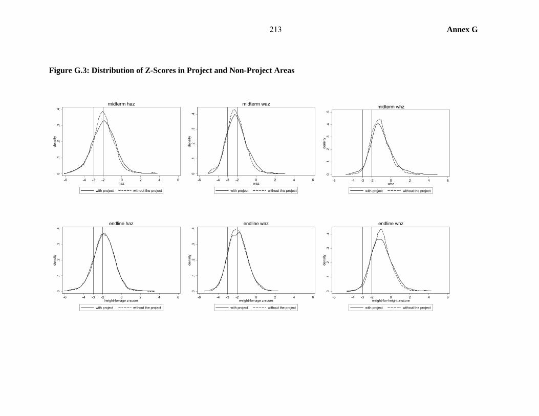
213 Annex G

Figure G.3: Distribution of Z-Scores in Project and Non-Project Areas

0.1

.2.3

.4de

nsity

-6 -4 -3 -2 0 2 4 6haz

with project without the project

midterm haz

0.1

.2.3

.4de

nsity

-6 -4 -3 -2 0 2 4 6waz


midterm waz

0.1

.2.3

.4.5

dens

ity

-6 -4 -3 -2 0 2 4 6whz


midterm whz

0.1

.2.3

.4de

nsity

-6 -4 -3 -2 0 2 4 6height-for-age z-score


endline haz

0.1

.2.3

.4de

nsity

-6 -4 -3 -2 0 2 4 6weight-for-age z-score


endline waz

0.1

.2.3

.4de

nsity

-6 -4 -3 -2 0 2 4 6weight-for-height z-score


endline whz

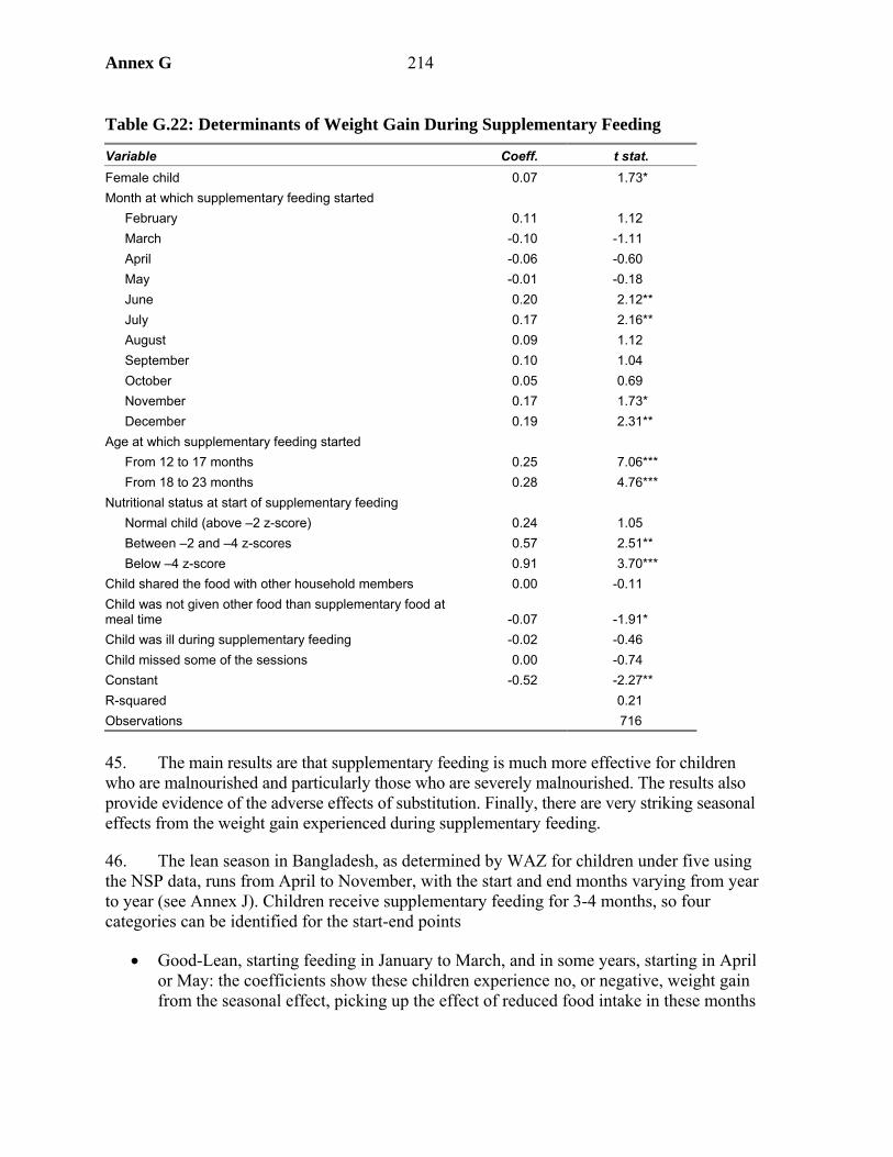
Annex G 214

Table G.22: Determinants of Weight Gain During Supplementary Feeding

Variable Coeff. t stat. Female child 0.07 1.73* Month at which supplementary feeding started

February 0.11 1.12 March -0.10 -1.11 April -0.06 -0.60 May -0.01 -0.18 June 0.20 2.12** July 0.17 2.16** August 0.09 1.12 September 0.10 1.04 October 0.05 0.69 November 0.17 1.73* December 0.19 2.31**

Age at which supplementary feeding started From 12 to 17 months 0.25 7.06*** From 18 to 23 months 0.28 4.76***

Nutritional status at start of supplementary feeding Normal child (above –2 z-score) 0.24 1.05 Between –2 and –4 z-scores 0.57 2.51** Below –4 z-score 0.91 3.70***

Child shared the food with other household members 0.00 -0.11 Child was not given other food than supplementary food at meal time -0.07 -1.91* Child was ill during supplementary feeding -0.02 -0.46 Child missed some of the sessions 0.00 -0.74 Constant -0.52 -2.27** R-squared 0.21 Observations 716

45. The main results are that supplementary feeding is much more effective for children who are malnourished and particularly those who are severely malnourished. The results also provide evidence of the adverse effects of substitution. Finally, there are very striking seasonal effects from the weight gain experienced during supplementary feeding.

46. The lean season in Bangladesh, as determined by WAZ for children under five using the NSP data, runs from April to November, with the start and end months varying from year to year (see Annex J). Children receive supplementary feeding for 3-4 months, so four categories can be identified for the start-end points

• Good-Lean, starting feeding in January to March, and in some years, starting in April or May: the coefficients show these children experience no, or negative, weight gain from the seasonal effect, picking up the effect of reduced food intake in these months

215 Annex G

• Lean-Lean, starting feeding in June to August, and in some years early September: the coefficients show a greater weight gain for children starting and finishing feeding in the lean season.

• Lean-Good, starting feeding September to November, and in some years August: as expected there is a positive weight gain for these children, partially reflecting greater food availability at the end of the period, this effect is greatest for children starting November as it takes time for the effect of increased food availability to feed through to improved WAZ.

• Good-Good, starting feeding in December and January, and in some years November: the coefficients for November and December are high reflecting the cumulative effect of three months of better food supply.

47. The regression results can be used to calculate the weight gain during supplementary feeding for a child with average characteristics. Table G.22, shows the results, varying only the characteristic shown. Children who enter the program more malnourished gain more from the program than better nourished children.1 Children under 12 months appear to show negligible gain in WAZ during the program, compared to close to 0.3 WAZ for older children. However, as shown in Figure G.4, the NSP data show that the WAZ falls for children across Bangladesh at a rate of about 0.5 WAZ over a three-month period. This occurs since the curves in the growth monitoring chart are very steep for children aged below 12 months (Figure G.5), so that substantial weight gain is needed to not fall further below the curve. Hence, compared to this reference group, a zero gain of WAZ is actually a gain of 0.5 WAZ, which is not insubstantial.

48. Finally, Table G.23 reports regressions using the BINP endline data for WAZ and midterm and HAZ at endline, these measures being selected since they are the ones for which a significant impact appears in the double difference and PSM analyses. A project dummy is used, interacted with various characteristics. Program activities cannot be used as they would suffer from selection bias (they are indeed found to have a negative effect when introduced into the regression). The project dummies are significant, though not large. The project mutes the advantage of more educated women, that is, nutritional counseling is substituting for education, and to a lesser extent offsetting the advantages of higher economic status. It also reduced the “daughter-in-law” disadvantage.

1. The category of normally nourished is not shown in Table G.22 as they constitute less than 1 percent of program participants.

Table G.22: Weight Gain from Supplementary Feeding for Different Categories of Children

Malnourished Severely malnourished

Very severely malnourished

-0.11 0.22 0.56 <12 months 12-17 months 17-23 months 0.02 0.27 0.29

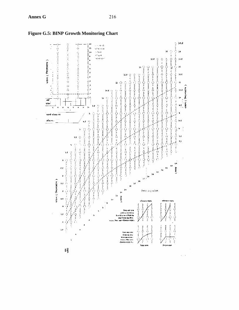
Annex G 216

Figure G.5: BINP Growth Monitoring Chart

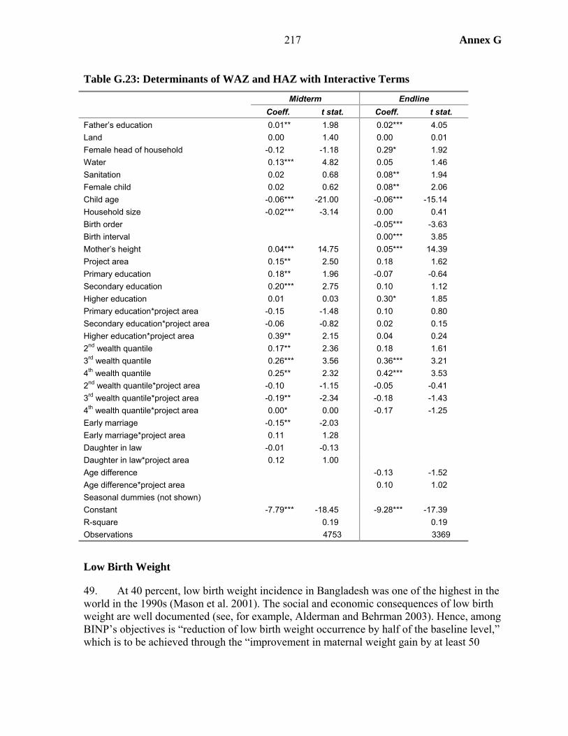
217 Annex G

Table G.23: Determinants of WAZ and HAZ with Interactive Terms

Midterm Endline Coeff. t stat. Coeff. t stat.

Father’s education 0.01** 1.98 0.02*** 4.05 Land 0.00 1.40 0.00 0.01 Female head of household -0.12 -1.18 0.29* 1.92 Water 0.13*** 4.82 0.05 1.46 Sanitation 0.02 0.68 0.08** 1.94 Female child 0.02 0.62 0.08** 2.06 Child age -0.06*** -21.00 -0.06*** -15.14 Household size -0.02*** -3.14 0.00 0.41 Birth order -0.05*** -3.63 Birth interval 0.00*** 3.85 Mother’s height 0.04*** 14.75 0.05*** 14.39 Project area 0.15** 2.50 0.18 1.62 Primary education 0.18** 1.96 -0.07 -0.64 Secondary education 0.20*** 2.75 0.10 1.12 Higher education 0.01 0.03 0.30* 1.85 Primary education*project area -0.15 -1.48 0.10 0.80 Secondary education*project area -0.06 -0.82 0.02 0.15 Higher education*project area 0.39** 2.15 0.04 0.24 2nd wealth quantile 0.17** 2.36 0.18 1.61 3rd wealth quantile 0.26*** 3.56 0.36*** 3.21 4th wealth quantile 0.25** 2.32 0.42*** 3.53 2nd wealth quantile*project area -0.10 -1.15 -0.05 -0.41 3rd wealth quantile*project area -0.19** -2.34 -0.18 -1.43 4th wealth quantile*project area 0.00* 0.00 -0.17 -1.25 Early marriage -0.15** -2.03 Early marriage*project area 0.11 1.28 Daughter in law -0.01 -0.13 Daughter in law*project area 0.12 1.00 Age difference -0.13 -1.52 Age difference*project area 0.10 1.02 Seasonal dummies (not shown) Constant -7.79*** -18.45 -9.28*** -17.39 R-square 0.19 0.19 Observations 4753 3369

Low Birth Weight

49. At 40 percent, low birth weight incidence in Bangladesh was one of the highest in the world in the 1990s (Mason et al. 2001). The social and economic consequences of low birth weight are well documented (see, for example, Alderman and Behrman 2003). Hence, among BINP’s objectives is “reduction of low birth weight occurrence by half of the baseline level,” which is to be achieved through the “improvement in maternal weight gain by at least 50

Annex G 218

percent in at least 50 percent of the pregnant women”2 (World Bank 1995). These goals are to be achieved through nutrition education and food supplementation. All pregnant women of project villages are regularly weighed and counseled on the proper diet to follow in order to gain the necessary weight. Women identified as malnourished are given a daily food supplement from the first screening to the sixth month of lactation after birth.

Concepts and Definitions

50. Low birth weight, i.e., below 2,500 grams, is determined by two factors: gestational age at birth and intrauterine growth (WHO 1995). In the first case, the infant has a low birth weight because he or she was born prematurely, which does not imply a failure to grow during pregnancy. In the second case, the infant has a low birth weight because its intrauterine growth was impaired by the health and nutrition history of the mother (Intrauterine Growth Retardation, IUGR). The two types of low birth weight should be considered separately because they have different determinants and different consequences for child health. Premature birth is not affected by malnutrition, and infants born prematurely have better chances of surviving and catching up in infancy and childhood than those children with low birth weight resulting from IUGR. In order to isolate birth weight from premature birth effects, infant weight can be measured against the weight for gestational age of a reference population.

51. Gestational weight gain has four components: fat stores, breast and uterine growth, volume of plasma, and fetus (Kramer 1987). Mother’s fat stores are the only component of weight gain that has an influence on the growth of the fetus. But mothers have different fat stores levels before pregnancy, which has two important implications: (a) heavier mothers need lower weight gains during pregnancy, and (b) the effect of additional food intake has a larger effect on infants of mothers that are thinner before pregnancy. The Institute of Medicine (1990) has produced charts of optimal gestational weight gain for women of different BMI, based on a sample of U.S. women who delivered infants of normal weight. These charts recommend a weekly gain of 0.4 kilograms during the second and third trimester for woman of normal pre-pregnant BMI, and of 0.5 kilograms for women who are underweight.

52. It is common in Bangladesh for women to reduce food intake during pregnancy, a practice often referred to as “eating down.” This practice is well documented for India and is explained by the mothers’ intention to reduce infant body size, thus facilitating delivery.3 CARE (Vemury 1981) conducted a survey study on food habits in six developing countries and found that some 60 percent of the 700 Bangladeshi women interviewed believed that pregnant women should eat less during pregnancy. The reasons given were the prevention of difficult delivery and customary beliefs (see also Hossain and Choudury 1987). The project document and Bangladeshi women thus share the belief that infant body size can be changed during pregnancy by eating more or less than usual. They do not have the same view, however, on the delivery outcome. Larger infants, according to the project, do not create an

2. These are the quantitative targets defined in the project document (World Bank 1995, p. 15). It is not clear how the latter can be measured, since the same women will not be pregnant at midterm and endline as were at baseline. Karim et al. (2003) rephrased the target as “improvement of weight gain to 7.0 kg. in at least 50% of pregnant women.”

3. See in particular the reviews by Chatterjee (1991) and Nag (1994).

219 Annex G

additional risk at delivery. However, the review of knowledge on nutrition during pregnancy done by the Institute of Medicine (1990) documents that in Western countries before World War II, women were commonly advised during pregnancy to avoid excessive weight gain or to restrict their food intake, concluding that “in a period when maternal mortality was extremely high and cesarean deliveries were a desperate alternative, limitation of fetal size by restricting maternal food intake was an understandable goal.” Maternal mortality at delivery is very high in Bangladesh (estimated in the range of 320 to 400 per 100,000 live births for the period 1998 to 20014). And nearly 80 percent of these deaths are due to obstetric causes, like obstructed labor, abortion, and eclampsia (Faveau et al. 1988). Sixty percent of Bangladshi women reported a complication during pregnancy, delivery, or after delivery (NIPRT 2002). Yet, very few women in Bangladesh deliver in hospitals or are assisted by professionals. The belief of “eating down” is thus understandable, and its effects on delivery are in fact not fully understood. However, some studies (quoted in Pojda and Kelley 2000, p. 24) report that increases in head circumference due to food supplements does not increase mortality risk from obstructed labor.5

Project Impact

53. This section uses the data collected for the BINP evaluation at midterm and endline. The baseline survey did not collect information on birth weight and pregnancy weight gains. The midterm and endline surveys are cross-sections using different samples for children, newborn, and mothers anthropometric measurements. Two problems arise when comparing the nutritional outcomes of project and control areas. First, not all women interviewed in BINP areas participated in project activities. Second, project and control areas may differ in some important determinants of nutritional outcomes independently of project implementation. The second problem is handled through the difference and double difference approaches (see appendix 1).

54. Table G.24 shows the difference, and the difference in difference, in the percentage of low birth weight and in the average newborn weight between project and control areas. Data on birth weight were not available at the baseline and therefore the table only contains the differences between the midterm and the endline. Low birth weight is defined as a birth weight below 2.5 kilograms. The ratio of birth weight over the median weight of a reference population of the same sex and gestational month is used as mean weight score.6

4. Estimates by NIPRT (2002).

5. It is not clear, however whether the absence of an effect of food supplementation program on maternal mortality risk is the result of the absence of an effect of larger body size on delivery, or of the absence of an effect of food supplementation on body size.

6. In order to measure intrauterine growth it is necessary to adjust birth weight by gestational age at birth in order to isolate the component influenced by nutrition. Several reference populations are available. The one used here are a Canadian reference population (Kramer 2001) for birth weight for gestational age. BINP data report only the month of birth as the 8th, 9th, or 10th, while reference weights by gestational age are normally reported by week. The recommended weight at the 40th week of gestation is used as a reference for the 9th month reported weight; the 39th week for the 8th month and the 41st week for the 10th month, assuming that the distribution of births in the 8th and 10th months tend to concentrate around the 40th week. This ratio is not very precise, but it is better to adjust for sex, and partially for gestational age, than not adjusting at all.

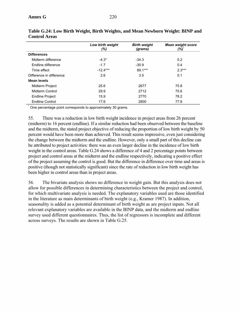
Annex G 220

Table G.24: Low Birth Weight, Birth Weights, and Mean Newborn Weight: BINP and Control Areas

Low birth weight (%)

Birth weight (grams)

Mean weight score(%)*

Differences Midterm difference -4.3* -34.3 0.2 Endline difference -1.7 -30.9 0.4 Time effect -12.4*** 89.1*** 2.3***

Difference in difference 2.6 3.5 0.1 Mean levels

Midterm Project 25.6 2677 75.8 Midterm Control 29.9 2712 75.6 Endline Project 15.9 2770 78.2 Endline Control 17.6 2800 77.8

* One percentage point corresponds to approximately 30 grams. 55. There was a reduction in low birth weight incidence in project areas from 26 percent (midterm) to 16 percent (endline). If a similar reduction had been observed between the baseline and the midterm, the stated project objective of reducing the proportion of low birth weight by 50 percent would have been more than achieved. This result seems impressive, even just considering the change between the midterm and the endline. However, only a small part of this decline can be attributed to project activities: there was an even larger decline in the incidence of low birth weight in the control areas. Table G.24 shows a difference of 4 and 2 percentage points between project and control areas at the midterm and the endline respectively, indicating a positive effect of the project assuming the control is good. But the difference in difference over time and areas is positive (though not statistically significant) since the rate of reduction in low birth weight has been higher in control areas than in project areas.

56. The bivariate analysis shows no difference in weight gain. But this analysis does not allow for possible differences in determining characteristics between the project and control, for which multivariate analysis is needed. The explanatory variables used are those identified in the literature as main determinants of birth weight (e.g., Kramer 1987). In addition, seasonality is added as a potential determinant of birth weight as are project inputs. Not all relevant explanatory variables are available in the BINP data, and the midterm and endline survey used different questionnaires. Thus, the list of regressors is incomplete and different across surveys. The results are shown in Table G.25.

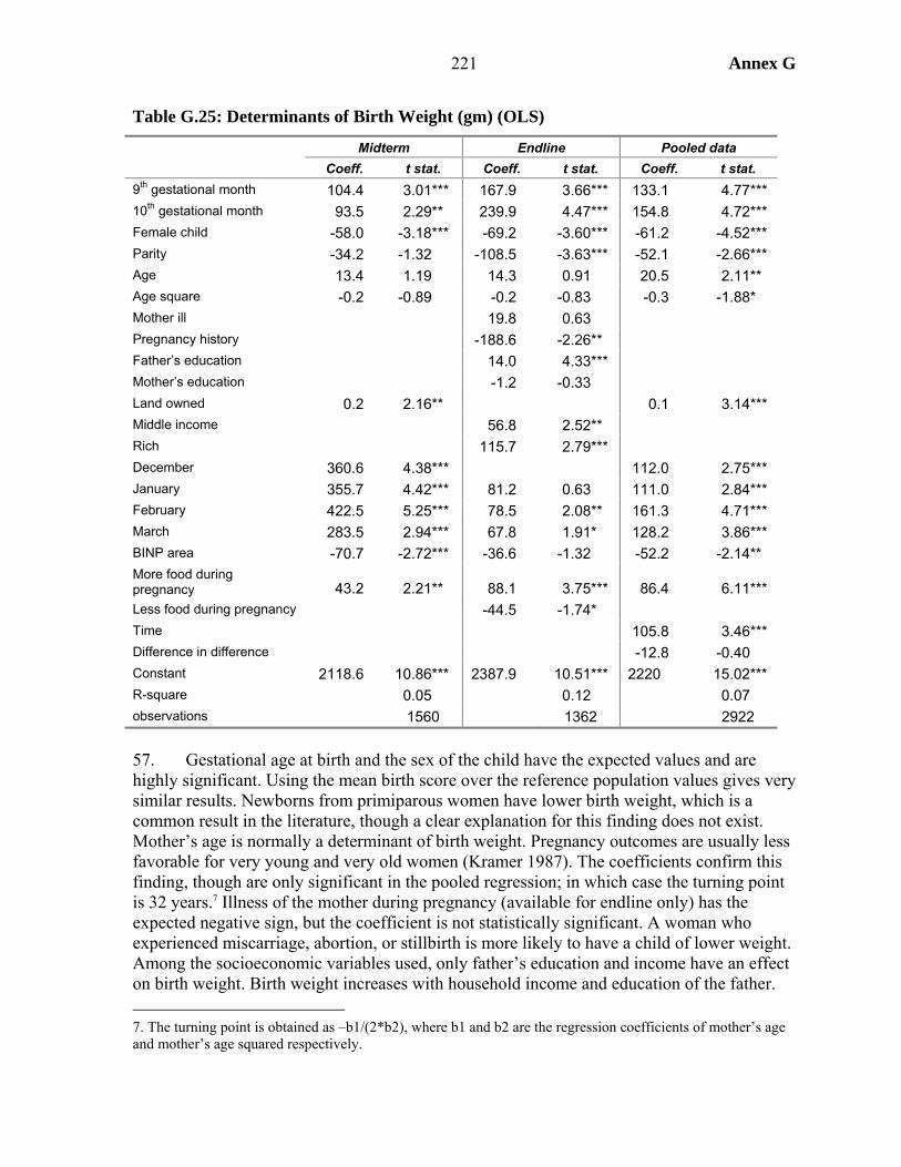
221 Annex G

Table G.25: Determinants of Birth Weight (gm) (OLS)

Midterm Endline Pooled data Coeff. t stat. Coeff. t stat. Coeff. t stat.

9th gestational month 104.4 3.01*** 167.9 3.66*** 133.1 4.77*** 10th gestational month 93.5 2.29** 239.9 4.47*** 154.8 4.72*** Female child -58.0 -3.18*** -69.2 -3.60*** -61.2 -4.52*** Parity -34.2 -1.32 -108.5 -3.63*** -52.1 -2.66*** Age 13.4 1.19 14.3 0.91 20.5 2.11** Age square -0.2 -0.89 -0.2 -0.83 -0.3 -1.88* Mother ill 19.8 0.63 Pregnancy history -188.6 -2.26** Father’s education 14.0 4.33*** Mother’s education -1.2 -0.33 Land owned 0.2 2.16** 0.1 3.14*** Middle income 56.8 2.52** Rich 115.7 2.79*** December 360.6 4.38*** 112.0 2.75*** January 355.7 4.42*** 81.2 0.63 111.0 2.84*** February 422.5 5.25*** 78.5 2.08** 161.3 4.71*** March 283.5 2.94*** 67.8 1.91* 128.2 3.86*** BINP area -70.7 -2.72*** -36.6 -1.32 -52.2 -2.14** More food during pregnancy 43.2 2.21** 88.1 3.75*** 86.4 6.11*** Less food during pregnancy -44.5 -1.74* Time 105.8 3.46*** Difference in difference -12.8 -0.40 Constant 2118.6 10.86*** 2387.9 10.51*** 2220 15.02*** R-square 0.05 0.12 0.07 observations 1560 1362 2922 57. Gestational age at birth and the sex of the child have the expected values and are highly significant. Using the mean birth score over the reference population values gives very similar results. Newborns from primiparous women have lower birth weight, which is a common result in the literature, though a clear explanation for this finding does not exist. Mother’s age is normally a determinant of birth weight. Pregnancy outcomes are usually less favorable for very young and very old women (Kramer 1987). The coefficients confirm this finding, though are only significant in the pooled regression; in which case the turning point is 32 years.7 Illness of the mother during pregnancy (available for endline only) has the expected negative sign, but the coefficient is not statistically significant. A woman who experienced miscarriage, abortion, or stillbirth is more likely to have a child of lower weight. Among the socioeconomic variables used, only father’s education and income have an effect on birth weight. Birth weight increases with household income and education of the father. 7. The turning point is obtained as –b1/(2*b2), where b1 and b2 are the regression coefficients of mother’s age and mother’s age squared respectively.

Annex G 222

Land ownership also has a positive and significant effect, but the value of the coefficient is negligible. The R-squareds are low in particular for the midterm model which contains only a small number of regressors. Important explanatory variables missing from the model include mother’s height and pre-pregnancy weight.

58. The month of measurement is included in the model to detect seasonal effects on birth weight. The effect is strong and the pattern clear. Birth weight is higher in the included months, December-March. However, there is a large difference in the effect of the seasonal variable between the two surveys which indicates that the model should be better specified. The implication is that mother’s nutrition is critical in the last months of pregnancy. However, the seasonal effect is much less relevant in project areas (shown by interacting the seasonal variables with the project dummy, results not shown here). The project tends to smooth out the seasonal pattern of mother’s nutrition. The implication is that if the data had been collected during the “hungry” season they would have probably shown a positive impact of the project on birth weights.

59. The model includes a variable taking the value of one if the mother says she ate more than usual during pregnancy, which is one channel for project impact if women change this practice in response to being in the project area. Women may have eaten more during pregnancy in the project areas both as a result of the availability of food supplementation and in response to the nutritional education against eating down. Whether the woman received food supplementation was also included in the model, but was not significant. This result presumably reflects attrition from leakage and substitution (see Tables G.15 and G.16) – it is only if the woman actually eats more that matters, which some women receiving food supplements do, but a sizeable number do not. “Eating more” increases birth weight by 44 grams in the midterm survey and by 88 grams in the endline. The effect is highly significant in both cases. The effect of “eating down” (mothers stating they ate less than usual during pregnancy) is also significant and negative, reducing birth weight by 45 grams (only available for endline). The effect of a mother changing from eating down to eating more is thus 133 grams. An increase of just over 80 grams from eating more is not very large, but is similar to the effect on birth weight observed in other projects where pregnant women were given food supplements.8 In addition, the effect is larger for women of poorer nutritional status. The interaction of the “eating more” dummy with the income level of the household of residence (results not shown) produces a much larger coefficient (+270 grams) for the “destitute” women.

60. BINP may have affected birth weight through other channels, such as the quality of diet. These channels are captured by the project dummy in the midterm and endline equations.9 However, this dummy is negative in both cases, though insignificant at endline. But interpreting this negative coefficient as an adverse project impact means assuming that

8. See the review of studies on the effect of supplementation project on low birth weight in Waterlow (1992) and Institute of Medicine (1990). These review report the following changes in birth weight: Guatemala (+100), Colombia (+180, but only for thin women), Gambia (+120, but only in hungry season), Chile (+60), Indonesia (no effect). No effect on birth weight was observed in similar projects carried out in Canada, Scotland, and the United States.

9. See appendix 2 for the interpretation of the BINP coefficient in different model specifications.

223 Annex G

all unobserved determinants of birth weight were the same in the project and control areas prior to the project. Pooling the data, and so estimating the double difference effect, allows us to control for these unobservables. In the pooled equation, the coefficients on the BINP area dummy are now unexplained area differences, with the project effect shown by the difference in difference coefficient (see appendix 1). This coefficient is negative but relatively small and very insignificant. There is a large and significant time effect on birth weight in both areas, where birth weight has increased on average by 100 grams, indicating a large autonomous change, most likely as a result of improving mother’s nutritional status.

61. The total project effect is calculated by combining both the effect through mother’s eating patterns and the project effect coefficient (the BINP dummy in the midterm and endline equations and the difference in difference coefficient for the pooled data). The results from the pooled regression suggest an increase in birth weight of just over 80 grams through eating more (on the assumption that a woman does eat more, which not all do), with no other project effects. The figure of 80 grams is thus an upper estimate of the average effect. This is an average effect, since it was also shown that the impact is greater during the lean season and higher for women poorer (and therefore probably less well nourished) women. The average impact on low birth weight is not large at all. What explains this relatively weak performance?

Project Impact on Pregnancy Weight Gain

62. The project aimed to increase birth weight by increasing mothers’ weight gains during pregnancy. The first hypothesis to explain the absence of a reduction in the incidence of low birth weight in project areas compared to control areas, is that mothers’ pregnancy weight did not increase as expected.

63. Figure G.5 plots weight gains of project and control areas for month of gestation compared to a reference population. The reference population is the one used by the Institute of Medicine (1990) for underweight women, defined as women of BMI below 19.8, which includes most the women in the sample. The lines for the project and control areas are obtained cumulating median weight gains at each month of gestation. Few observations are available for weight gains before the third month of gestation, therefore the curves before that date are not reliable. Both graphs show a growth pattern inferior to the reference population, and no difference between control and project at the midterm, though there is some difference at the endline. Similarly, Table G.26 shows the differences between areas and over time in mean weight gains. Weights were measured at one-month intervals for samples of pregnant women at different stages of gestation. The table shows a significant project effect and a positive project effect over time compared to control areas. However, as in the case of birth weight, these comparisons are of little use unless differences in the determinants of weight gain are allowed for with multivariate analysis.

Figure G.5: Mothers’ Weight Gain by Month of Gestation

Table G.26: Difference in Monthly Pregnancy Weight Gain Between Project and Control Areas

Grams Midterm difference 0.5 Endline difference 211.0*** Time effect -137.9 Difference in difference 210.4**

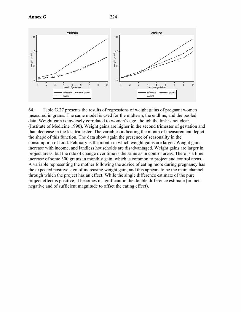
Annex G 224

05

1015

wei

ght g

ain

kg.

1 2 3 4 5 6 7 8 9month of gestation

reference projectcontrol

midterm

05

1015

wei

ght g

ain

kg.

1 2 3 4 5 6 7 8 9month of gestation

reference projectcontrol

endline

64. Table G.27 presents the results of regressions of weight gains of pregnant women measured in grams. The same model is used for the midterm, the endline, and the pooled data. Weight gain is inversely correlated to women’s age, though the link is not clear (Institute of Medicine 1990). Weight gains are higher in the second trimester of gestation and than decrease in the last trimester. The variables indicating the month of measurement depict the shape of this function. The data show again the presence of seasonality in the consumption of food. February is the month in which weight gains are larger. Weight gains increase with income, and landless households are disadvantaged. Weight gains are larger in project areas, but the rate of change over time is the same as in control areas. There is a time increase of some 300 grams in monthly gain, which is common to project and control areas. A variable representing the mother following the advice of eating more during pregnancy has the expected positive sign of increasing weight gain, and this appears to be the main channel through which the project has an effect. While the single difference estimate of the pure project effect is positive, it becomes insignificant in the double difference estimate (in fact negative and of sufficient magnitude to offset the eating effect).

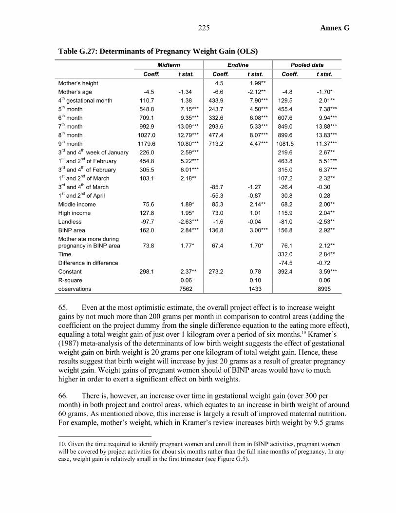
225 Annex G

Table G.27: Determinants of Pregnancy Weight Gain (OLS)

Midterm Endline Pooled data Coeff. t stat. Coeff. t stat. Coeff. t stat.

Mother’s height 4.5 1.99** Mother’s age -4.5 -1.34 -6.6 -2.12** -4.8 -1.70* 4th gestational month 110.7 1.38 433.9 7.90*** 129.5 2.01** 5th month 548.8 7.15*** 243.7 4.50*** 455.4 7.38*** 6th month 709.1 9.35*** 332.6 6.08*** 607.6 9.94*** 7th month 992.9 13.09*** 293.6 5.33*** 849.0 13.88*** 8th month 1027.0 12.79*** 477.4 8.07*** 899.6 13.83*** 9th month 1179.6 10.80*** 713.2 4.47*** 1081.5 11.37*** 3rd and 4th week of January 226.0 2.59*** 219.6 2.67** 1st and 2nd of February 454.8 5.22*** 463.8 5.51*** 3rd and 4th of February 305.5 6.01*** 315.0 6.37*** 1st and 2nd of March 103.1 2.18** 107.2 2.32** 3rd and 4th of March -85.7 -1.27 -26.4 -0.30 1st and 2nd of April -55.3 -0.87 30.8 0.28 Middle income 75.6 1.89* 85.3 2.14** 68.2 2.00** High income 127.8 1.95* 73.0 1.01 115.9 2.04** Landless -97.7 -2.63*** -1.6 -0.04 -81.0 -2.53** BINP area 162.0 2.84*** 136.8 3.00*** 156.8 2.92** Mother ate more during pregnancy in BINP area 73.8 1.77* 67.4 1.70* 76.1 2.12** Time 332.0 2.84** Difference in difference -74.5 -0.72 Constant 298.1 2.37** 273.2 0.78 392.4 3.59*** R-square 0.06 0.10 0.06 observations 7562 1433 8995

65. Even at the most optimistic estimate, the overall project effect is to increase weight gains by not much more than 200 grams per month in comparison to control areas (adding the coefficient on the project dummy from the single difference equation to the eating more effect), equaling a total weight gain of just over 1 kilogram over a period of six months.10 Kramer’s (1987) meta-analysis of the determinants of low birth weight suggests the effect of gestational weight gain on birth weight is 20 grams per one kilogram of total weight gain. Hence, these results suggest that birth weight will increase by just 20 grams as a result of greater pregnancy weight gain. Weight gains of pregnant women should of BINP areas would have to much higher in order to exert a significant effect on birth weights.

66. There is, however, an increase over time in gestational weight gain (over 300 per month) in both project and control areas, which equates to an increase in birth weight of around 60 grams. As mentioned above, this increase is largely a result of improved maternal nutrition. For example, mother’s weight, which in Kramer’s review increases birth weight by 9.5 grams

10. Given the time required to identify pregnant women and enroll them in BINP activities, pregnant women will be covered by project activities for about six months rather than the full nine months of pregnancy. In any case, weight gain is relatively small in the first trimester (see Figure G.5).

Annex G 226

per kilogram, has increased by an average 3.4 kilograms between the two surveys. Mother’s height, which in Kramer’s review increases birth weight by 8 grams/centimeter, has increased by two centimeters between the surveys. Hence, the difference over time in birth weights depends in large part on non-project effects.

67. It remains to be explained why gestational weight gain has not increased much more in project areas with respect to control areas. Two reasons are possible: (i) low participation rates, particularly by women most in need and, (ii) though women participate and receive the services, there are constraints that prevent the realization of the expected outcomes.

Cost Effectiveness

68. Table G.28 shows BINP project costs from 1996 through 2003 by main component from the implementation completion report (ICR). The Community-based Nutrition Component accounts for more than 50 percent of total project costs.

Table G.28: Project Costs in US$ Million (actuals)

US$ million % shares National Nutrition Component (NNC) 18.4 31.7 Community-based nutrition component (CBNC) 32.3 55.6 Inter-sectoral Nutrition program development (INC) 6.5 11.2 TOTAL BASELINE COST 57.3 Physical contingencies 3.4 5.9 Price contingencies 5.0 8.7 TOTAL PROJECT COST 65.7 100.0

69. Table G.29 shows the change in child malnutrition produced by the project as measured by PSM at the midterm and the endline, and the consequent percentage reductions of malnourished children.11

Table G.29: Reduction in Malnutrition at the Midterm and Endline Calculated Using PSM

Midterm Endline Z-score % change Z-score % change

Weight-for-age +0.13 -5.3 +0.05 -2.0 Height-for-age +0.10 -4.1 +0.03 -1.3

11. Percent changes in malnutrition are calculated using a probit function in the following way. If Z is the average z-score before the project and dZ is the change in the average z-score of Table 2, the percent reduction in malnutrition is obtained as )2()2( dZZZ +−−Φ−−−Φ . Malnutrition rates are calculated using -2 z-score as cutoff point (this includes mild and severe malnutrition).

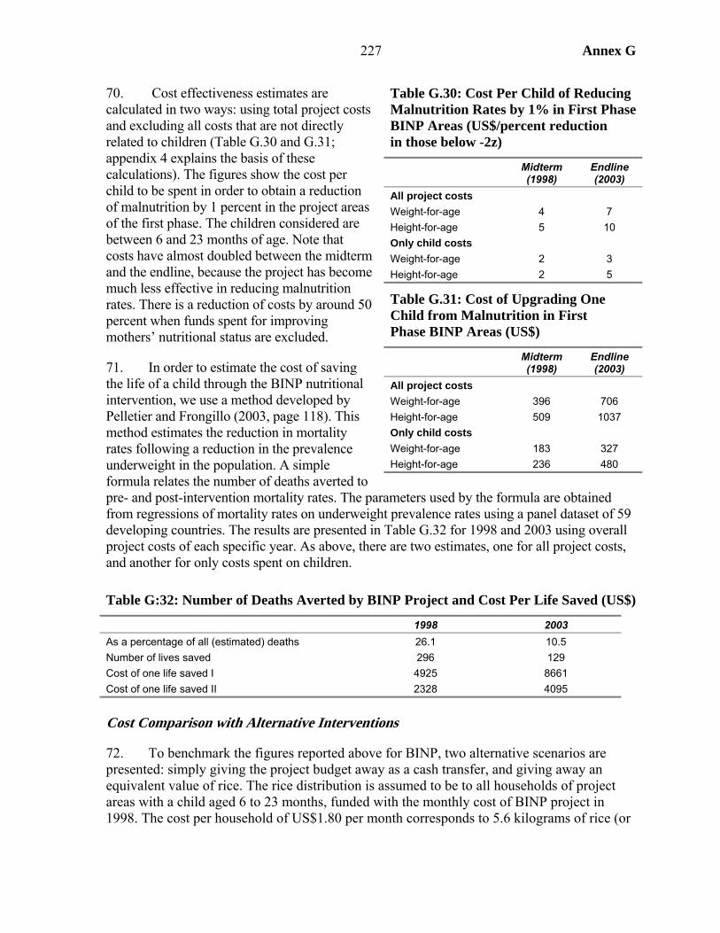
227 Annex G

70. Cost effectiveness estimates are calculated in two ways: using total project costs and excluding all costs that are not directly related to children (Table G.30 and G.31; appendix 4 explains the basis of these calculations). The figures show the cost per child to be spent in order to obtain a reduction of malnutrition by 1 percent in the project areas of the first phase. The children considered are between 6 and 23 months of age. Note that costs have almost doubled between the midterm and the endline, because the project has become much less effective in reducing malnutrition rates. There is a reduction of costs by around 50 percent when funds spent for improving mothers’ nutritional status are excluded.

71. In order to estimate the cost of saving the life of a child through the BINP nutritional intervention, we use a method developed by Pelletier and Frongillo (2003, page 118). This method estimates the reduction in mortality rates following a reduction in the prevalence underweight in the population. A simple formula relates the number of deaths averted to pre- and post-intervention mortality rates. The parameters used by the formula are obtained from regressions of mortality rates on underweight prevalence rates using a panel dataset of 59 developing countries. The results are presented in Table G.32 for 1998 and 2003 using overall project costs of each specific year. As above, there are two estimates, one for all project costs, and another for only costs spent on children.

Table G:32: Number of Deaths Averted by BINP Project and Cost Per Life Saved (US$)

1998 2003 As a percentage of all (estimated) deaths 26.1 10.5 Number of lives saved 296 129 Cost of one life saved I 4925 8661 Cost of one life saved II 2328 4095

Cost Comparison with Alternative Interventions

72. To benchmark the figures reported above for BINP, two alternative scenarios are presented: simply giving the project budget away as a cash transfer, and giving away an equivalent value of rice. The rice distribution is assumed to be to all households of project areas with a child aged 6 to 23 months, funded with the monthly cost of BINP project in 1998. The cost per household of US$1.80 per month corresponds to 5.6 kilograms of rice (or

Table G.30: Cost Per Child of Reducing Malnutrition Rates by 1% in First Phase BINP Areas (US$/percent reduction in those below -2z)

Midterm (1998)

Endline (2003)

All project costs Weight-for-age 4 7 Height-for-age 5 10 Only child costs Weight-for-age 2 3 Height-for-age 2 5

Table G.31: Cost of Upgrading One Child from Malnutrition in First Phase BINP Areas (US$)

Midterm (1998)

Endline (2003)

All project costs Weight-for-age 396 706 Height-for-age 509 1037 Only child costs Weight-for-age 183 327 Height-for-age 236 480

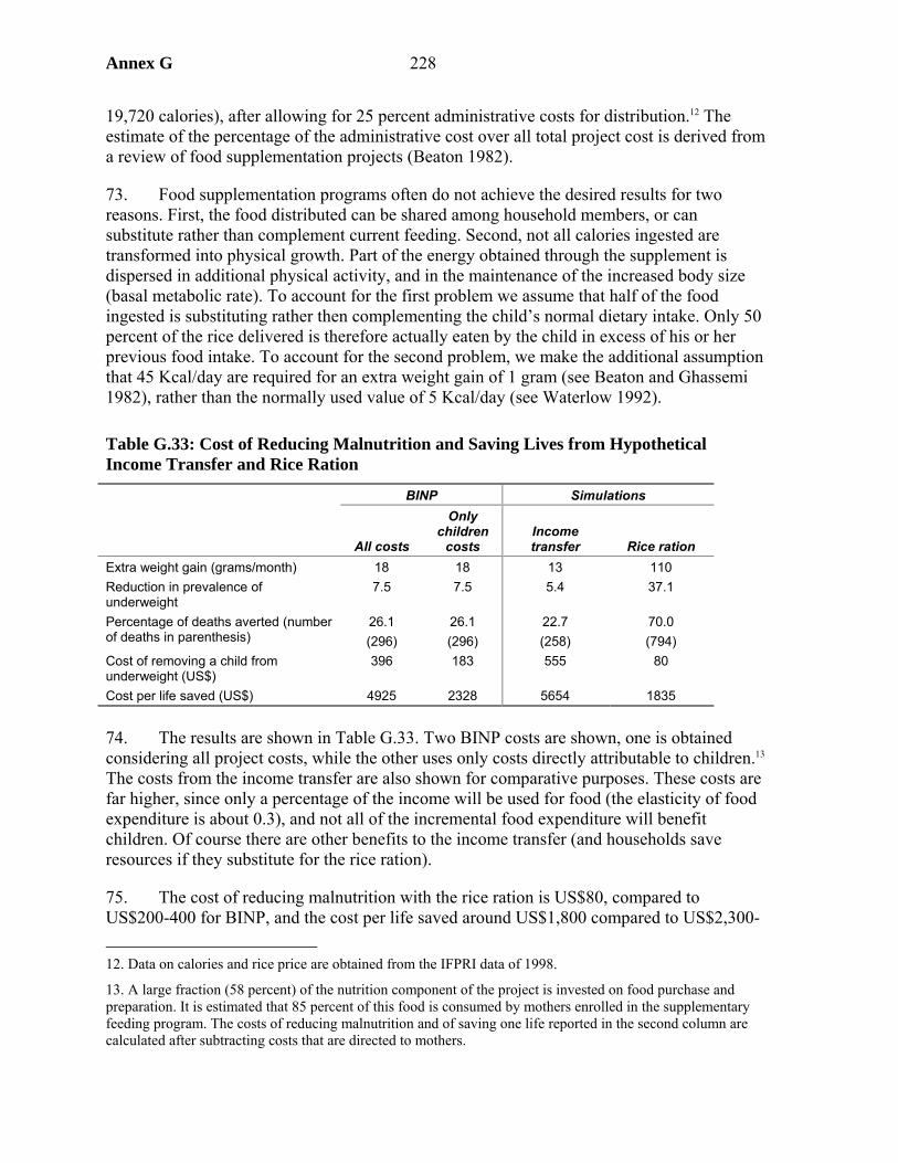
Annex G 228

19,720 calories), after allowing for 25 percent administrative costs for distribution.12 The estimate of the percentage of the administrative cost over all total project cost is derived from a review of food supplementation projects (Beaton 1982).

73. Food supplementation programs often do not achieve the desired results for two reasons. First, the food distributed can be shared among household members, or can substitute rather than complement current feeding. Second, not all calories ingested are transformed into physical growth. Part of the energy obtained through the supplement is dispersed in additional physical activity, and in the maintenance of the increased body size (basal metabolic rate). To account for the first problem we assume that half of the food ingested is substituting rather then complementing the child’s normal dietary intake. Only 50 percent of the rice delivered is therefore actually eaten by the child in excess of his or her previous food intake. To account for the second problem, we make the additional assumption that 45 Kcal/day are required for an extra weight gain of 1 gram (see Beaton and Ghassemi 1982), rather than the normally used value of 5 Kcal/day (see Waterlow 1992).

Table G.33: Cost of Reducing Malnutrition and Saving Lives from Hypothetical Income Transfer and Rice Ration

BINP Simulations

All costs

Only children

costs Income transfer Rice ration

Extra weight gain (grams/month) 18 18 13 110 Reduction in prevalence of underweight

7.5 7.5 5.4 37.1

Percentage of deaths averted (number of deaths in parenthesis)

26.1 (296)

26.1 (296)

22.7 (258)

70.0 (794)

Cost of removing a child from underweight (US$)

396 183 555 80

Cost per life saved (US$) 4925 2328 5654 1835

74. The results are shown in Table G.33. Two BINP costs are shown, one is obtained considering all project costs, while the other uses only costs directly attributable to children.13 The costs from the income transfer are also shown for comparative purposes. These costs are far higher, since only a percentage of the income will be used for food (the elasticity of food expenditure is about 0.3), and not all of the incremental food expenditure will benefit children. Of course there are other benefits to the income transfer (and households save resources if they substitute for the rice ration).

75. The cost of reducing malnutrition with the rice ration is US$80, compared to US$200-400 for BINP, and the cost per life saved around US$1,800 compared to US$2,300- 12. Data on calories and rice price are obtained from the IFPRI data of 1998.

13. A large fraction (58 percent) of the nutrition component of the project is invested on food purchase and preparation. It is estimated that 85 percent of this food is consumed by mothers enrolled in the supplementary feeding program. The costs of reducing malnutrition and of saving one life reported in the second column are calculated after subtracting costs that are directed to mothers.

229 Annex G

5,000 for BINP. Hence, BINP does not compare favorably with simply spending project resources of buying rice for children in the project area. The argument against such an approach is that it implies a permanent subsidy, whereas behavior change should become self-sustaining once affected. However, the evidence shows limited success in behavior change, partly as resource constraints prevent recommended changes from being put into practice. Moreover, there may be lower cost models of BCC given the pervasive presence of NGOs, women’s groups, and health and family planning officials,14 plus media saturation, which has proved successful in conveying other messages

14. Use of existing government workers, or local level voluntary workers, was ruled out of the BINP design on account of the workload. But a large part of this workload relates to growth monitoring rather than BCC.

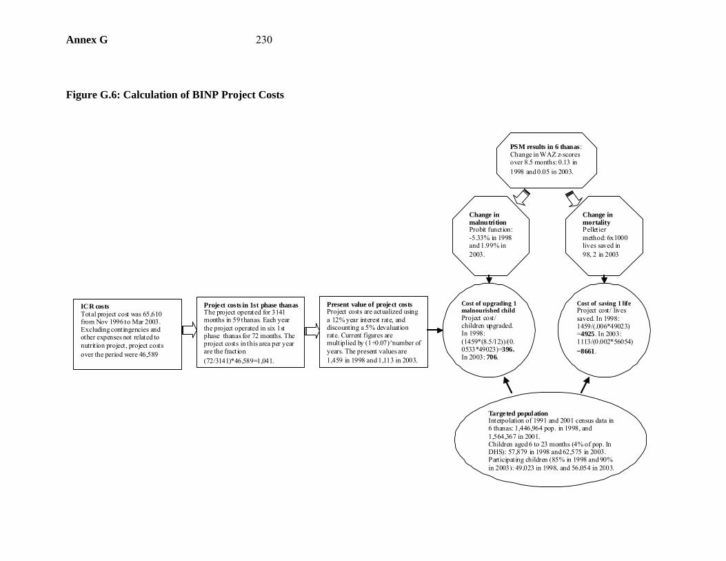
Annex G 230

Figure G.6: Calculation of BINP Project Costs

ICR costs Total project cost was 65,610 from Nov 1996 to Mar 2003. Excluding contingencies and other expenses not related to nutrit ion project, project costs over the period were 46,589

Project costs in 1st phase thanasThe project operated for 3141 months in 59 thanas. Each year the project operated in six 1st phase thanas for 72 months. The project costs in this area per year are the fraction (72/3141)*46,589=1,041.

Present value of project costsProject costs are actualized using a 12% year interest rate, and discounting a 5% devaluation rate. Current figures are multiplied by (1+0.07) n̂umber of years. The present values are 1,459 in 1998 and 1,113 in 2003.

PSM results in 6 thanas:Change in WAZ z-scores over 8.5 months: 0.13 in 1998 and 0.05 in 2003.

Change in mortality Pelletier method: 6x1000 lives saved in 98, 2 in 2003

Change in malnutrition Probit function: -5.33% in 1998 and 1.99% in 2003.

Targeted populationInterpolation of 1991 and 2001 census data in 6 thanas: 1,446,964 pop. in 1998, and 1,564,367 in 2001. Children aged 6 to 23 months (4% of pop. In DHS): 57,879 in 1998 and 62,575 in 2003. Participating children (85% in 1998 and 90% in 2003): 49,023 in 1998, and 56,054 in 2003.

Cost of upgrading 1 malnourished child Project cost/ children upgraded. In 1998: (1459*(8.5/12))/(0.0533*49023)=396. In 2003: 706.

Cost of saving 1 life Project cost/ lives saved. In 1998: 1459/(.006*49023)=4925. In 2003: 1113/(0.002*56054)=8661.

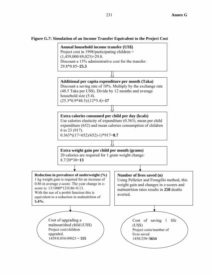
231 Annex G

Figure G.7: Simulation of an Income Transfer Equivalent to the Project Cost

Annual household income transfer (US$) Project cost in 1998/participating children = (1,459,000/49,023)=29.8. Discount a 15% administrative cost for the transfer: 29.8*0.85=25.3

Extra weight gain per child per month (grams) 20 calories are required for 1 gram weight change: 8.7/20*30=13

Extra calories consumed per child per day (kcals) Use calories elasticity of expenditure (0.363), mean per child expenditure (652) and mean calories consumption of children 6 to 23 (917). 0.363*((17+652)/652)-1)*917=8.7

Additional per capita expenditure per month (Taka) Discount a saving rate of 10%. Multiply by the exchange rate (48.5 Taka per US$). Divide by 12 months and average household size (5.4). (25.3*0.9*48.5)/(12*5.4)=17

Reduction in prevalence of underweight (%) 1 kg weight gain is required for an increase of 0.86 in average z-score. The year change in z-score is: 13/1000*12/0.86=0.13. With the use of a probit function this is equivalent to a reduction in malnutrition of 5.4%.

Number of lives saved (n) Using Pelletier and Frongillo method, this weight gain and changes in z-scores and malnutrition rates results in 258 deaths averted.

Cost of upgrading a malnourished child (US$) Project cost/children upgraded. 1459/0.054/49023 = 555

Cost of saving 1 life (US$) Project costs/number of lives saved. 1458/258=5654

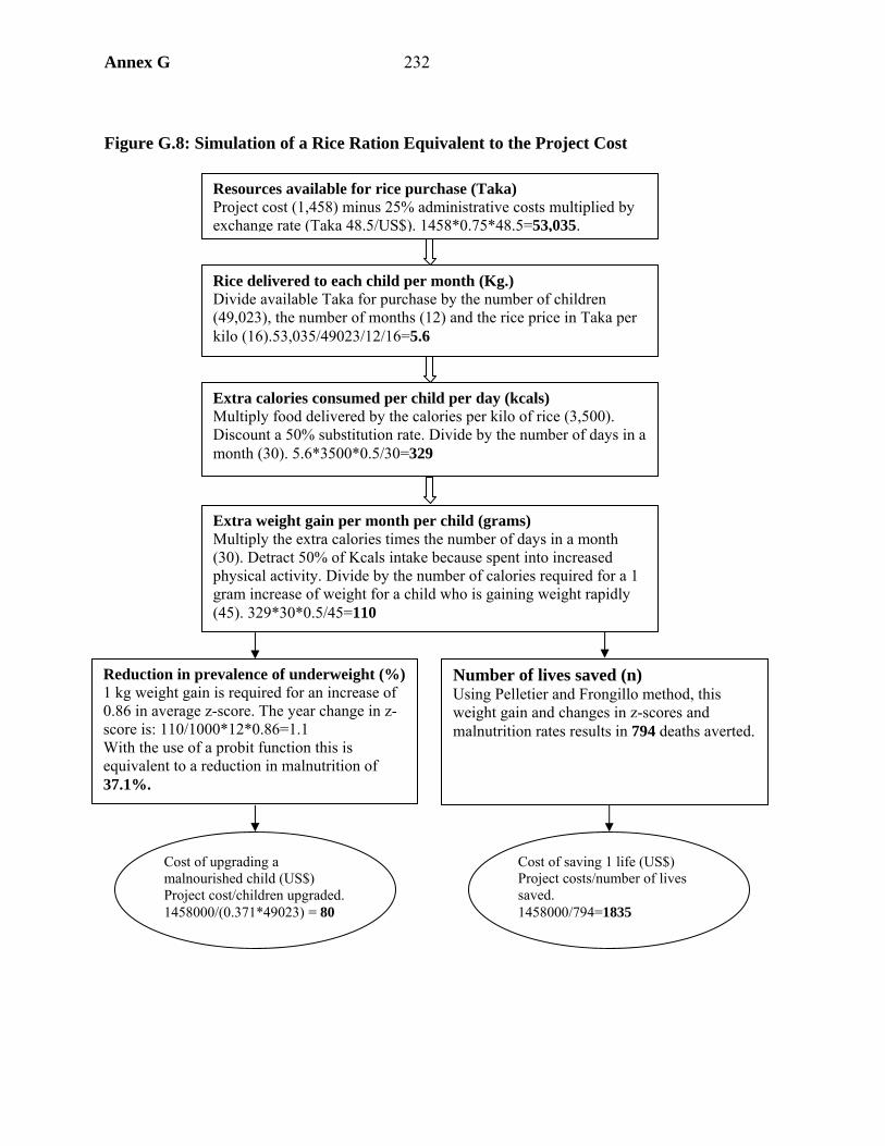
Annex G 232

Figure G.8: Simulation of a Rice Ration Equivalent to the Project Cost

Reduction in prevalence of underweight (%)1 kg weight gain is required for an increase of 0.86 in average z-score. The year change in z-score is: 110/1000*12*0.86=1.1 With the use of a probit function this is equivalent to a reduction in malnutrition of 37.1%.

Number of lives saved (n) Using Pelletier and Frongillo method, this weight gain and changes in z-scores and malnutrition rates results in 794 deaths averted.

Cost of upgrading a malnourished child (US$) Project cost/children upgraded. 1458000/(0.371*49023) = 80

Cost of saving 1 life (US$) Project costs/number of lives saved. 1458000/794=1835

Rice delivered to each child per month (Kg.) Divide available Taka for purchase by the number of children (49,023), the number of months (12) and the rice price in Taka per kilo (16).53,035/49023/12/16=5.6

Extra weight gain per month per child (grams)Multiply the extra calories times the number of days in a month (30). Detract 50% of Kcals intake because spent into increased physical activity. Divide by the number of calories required for a 1 gram increase of weight for a child who is gaining weight rapidly (45). 329*30*0.5/45=110

Extra calories consumed per child per day (kcals)Multiply food delivered by the calories per kilo of rice (3,500). Discount a 50% substitution rate. Divide by the number of days in a month (30). 5.6*3500*0.5/30=329

Resources available for rice purchase (Taka) Project cost (1,458) minus 25% administrative costs multiplied by exchange rate (Taka 48.5/US$). 1458*0.75*48.5=53,035.

233 Annex G

Conclusions

Child Nutritional Outcomes

76. Overall project impact on child nutritional outcomes appears disappointing despite high levels of participation in project activities. Although participation was high it was lower in more traditional thanas, which was partly a result of the project not having a broader target audience encompassing all key decisionmakers. Lack of decision-making power of participants was also a factor behind the knowledge-practice gap, though lack of resources and time played a larger part. There were other weak links in the chain, notably poor targeting, so that some eligible children did not receive feeding, and mothers and some pregnant women did not receive nutritional counseling.

Low Birth Weight

77. Low birth weight is a correlate of a child’s subsequent nutritional and health status, and so of mortality. BINP addresses low birth weight through increasing pregnancy weight gain by discouraging eating down and provided food supplements to malnourished women. BINP aimed to reduce “low birth weight occurrence by half of the baseline level” through the “improvement in maternal weight gain by at least 50 percent in at least 50 percent of the pregnant women.” The BINP evaluation found that the pregnancy weight gain target was achieved, though that of reducing low birth weight was not. However, the BINP evaluation dataset shows that there was an even larger increase in pregnancy weight gain in the control areas than in the project areas, suggesting that outside factors accounted for these improvements. Greater food availability has improved mothers’ pre-pregnancy nutritional status, as shown by rising BMI in both project and control areas, and it is this which has been the main driving force behind greater pregnancy weight gain.

78. There has been a project effect, but it has been relatively small. Multivariate analysis shows a small project effect on both pregnancy weight gain and low birth weight, mainly through discouraging the practice of eating less during pregnancy (eating down), assisted by providing feeding supplementation to pregnant women with less than normal body mass index. These effects are greater for more disadvantaged (and so presumably less well-nourished) women and during the lean season.

79. Potential beneficial impacts of the project are muted for reasons of poor targeting, failure to amend eating practices even when the message is got across (the knowledge-practice gap) and the leakage and substitution of supplementary feeding. It is shown that resource constrained women are more likely to have a knowledge-practice gap, supporting the argument that lack of income is sometimes the binding constraint on nutritional practices rather than lack of knowledge.

How Well Did the Causal Chain Operate?

80. BINP succeeded in achieving high levels of participation in its activities in project areas, enrolled large numbers in supplementary feeding, brought about significant increases in nutritional knowledge and associated changes in practice. However, nutritional outcomes in terms of low birth weight have been disappointing. While child nutrition, especially for

Annex G 234

children participating in supplementary feeding, appears to have been better, the overall difference in performance compared to the control is not great.

81. The longer the causal chain, the more likely it is that final outcomes will not be realized on account of missing or weak links in the chain. There were two missing links in the BINP chain: the first was the relative neglect of some key decisionmakers regarding nutritional choices (men and mothers-in-law), and the second the focus on pregnancy weight gain rather than pre-pregnancy nutritional status. Participation levels of the target audience were high, but many women escaped exposure to nutritional messages, and there was a high Type I error in the feeding programs (see Table G.34). A knowledge practice gap persisted, so many women did not put the advice they received into practice, especially if they were resource or time constrained. Those receiving supplementary feeding often shared it with others or substituted it for their regular foodstuffs. This list of weak links in the chain explain why project impact was muted by the time final outcomes are considered. While attention can be paid to each of these weak links, the BINP experience does demonstrate the difficulty of implementing complex designs.

Should BINP be Expanded Nationally?

82. Despite recent progress, Bangladesh has continuing high levels of malnutrition. Several factors lie behind improving nutrition, notably improved agricultural performance. Nonetheless, there appears a case for direct nutritional interventions. But in its current form, BINP has had a rather meager impact on nutritional outcomes, especially in comparison to its cost. There are two ways to respond to these findings. The first would be to attempt to improve project effectiveness by strengthening the causal chain. The most plausible way of doing this would be to target resources more finely, toward less well nourished mothers and children, with a larger supplement in the lean season. The alternative is a less sophisticated form of nutritional program, such as a rice ration. Although such schemes are no longer in fashion, the analysis shows that such a program would be no more expensive than scaling BINP up nationally and have a larger nutritional impact.

235 Annex G

Table G.34: Links in the Causal Chain

Assumption Children Mothers Attend growth monitoring sessions

Over 90 percent of children attend growth monitoring sessions

Over 70 percent participate in monitoring pregnancy weight gain

Targeting criteria correctly applied; participants stay in program to receive food

Nearly two-thirds of eligible children not fed (reasons: don’t attend growth monitoring in first place, wrong application of targeting criteria, drop out of feeding)

60 percent of eligible women not receiving supplementary feeding

Acquire knowledge and put it into practice

One-third of mothers of children receiving supplementary feeding do not receive nutritional counseling. There is a knowledge practice gap (see mothers).

There is a knowledge-practice gap, driven by material resource or time constraints.

No leakage or substitution One-quarter of children fed at home, increasing possibility of both leakage and substitution.

One-third admit sharing food, and there is substitution for those who do not. At most, 40 percent of eligible women receive full supplementation.

Feeding and nutritional advice have an impact on nutritional status

Supplementary feeding has a positive impact on child nutritional status, especially for the most malnourished children. There is only weak evidence of any impact from nutritional counseling.

Pregnancy weight gain is too little to have a notable impact on low birth weight, except for most malnourished mothers. Moreover, mother’s pre-pregnancy nutritional status is more important than pregnancy weight gain. Consequently, birth weight gains are slight, though greater for children of severely malnourished mothers. Eating more during pregnancy is the main channel for both pregnancy weight gain and higher birth weight.

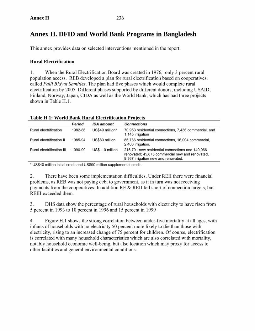
Annex H 236

Annex H. DFID and World Bank Programs in Bangladesh

This annex provides data on selected interventions mentioned in the report.

Rural Electrification

1. When the Rural Electrification Board was created in 1976, only 3 percent rural population access. REB developed a plan for rural electrification based on cooperatives, called Palli Bidyut Samities. The plan had five phases which would complete rural electrification by 2005. Different phases supported by different donors, including USAID, Finland, Norway, Japan, CIDA as well as the World Bank, which has had three projects shown in Table H.1.

Table H.1: World Bank Rural Electrification Projects Period IDA amount Connections Rural electrification 1982-86 US$49 million* 70,953 residential connections, 7,436 commercial, and

1,145 irrigation Rural electrification II 1985-94 US$80 million 85,766 residential connections, 16,004 commercial,

2,406 irrigation. Rural electrification III 1990-99 US$110 million 216,791 new residential connections and 140,066

renovated; 45,875 commercial new and renovated, 9,367 irrigation new and renovated.

* US$40 million initial credit and US$90 million supplemental credit. 2. There have been some implementation difficulties. Under REII there were financial problems, as REB was not paying debt to government, as it in turn was not receiving payments from the cooperatives. In addition RE & REII fell short of connection targets, but REIII exceeded them.

3. DHS data show the percentage of rural households with electricity to have risen from 5 percent in 1993 to 10 percent in 1996 and 15 percent in 1999

4. Figure H.1 shows the strong correlation between under-five mortality at all ages, with infants of households with no electricity 50 percent more likely to die than those with electricity, rising to an increased change of 75 percent for children. Of course, electrification is correlated with many household characteristics which are also correlated with mortality, notably household economic well-being, but also location which may proxy for access to other facilities and general environmental conditions.

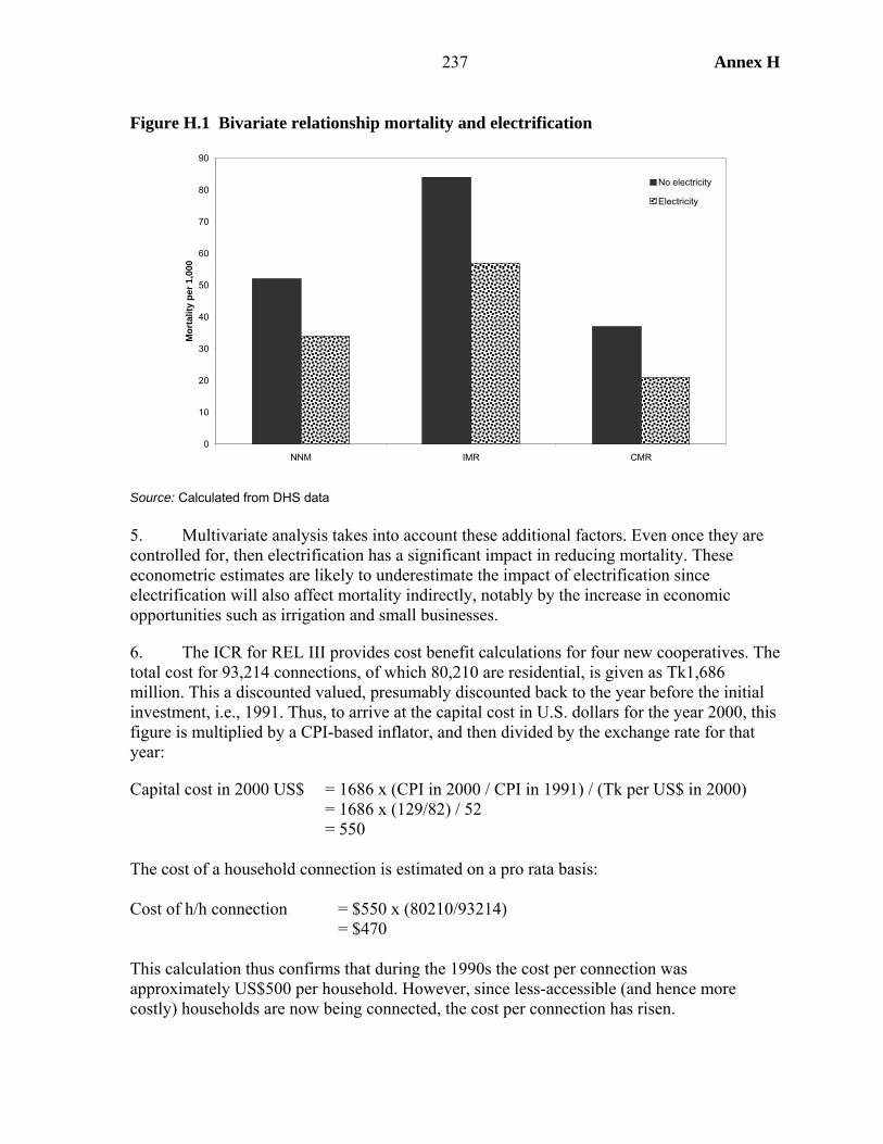
237 Annex H

0

10

20

30

40

50

60

70

80

90

NNM IMR CMR

Mor

talit

y pe

r 1,0

00No electricity

Electricity

Figure H.1 Bivariate relationship mortality and electrification

Source: Calculated from DHS data 5. Multivariate analysis takes into account these additional factors. Even once they are controlled for, then electrification has a significant impact in reducing mortality. These econometric estimates are likely to underestimate the impact of electrification since electrification will also affect mortality indirectly, notably by the increase in economic opportunities such as irrigation and small businesses.

6. The ICR for REL III provides cost benefit calculations for four new cooperatives. The total cost for 93,214 connections, of which 80,210 are residential, is given as Tk1,686 million. This a discounted valued, presumably discounted back to the year before the initial investment, i.e., 1991. Thus, to arrive at the capital cost in U.S. dollars for the year 2000, this figure is multiplied by a CPI-based inflator, and then divided by the exchange rate for that year:

Capital cost in 2000 US$ = 1686 x (CPI in 2000 / CPI in 1991) / (Tk per US$ in 2000) = 1686 x (129/82) / 52 = 550 The cost of a household connection is estimated on a pro rata basis: Cost of h/h connection = $550 x (80210/93214) = $470 This calculation thus confirms that during the 1990s the cost per connection was approximately US$500 per household. However, since less-accessible (and hence more costly) households are now being connected, the cost per connection has risen.

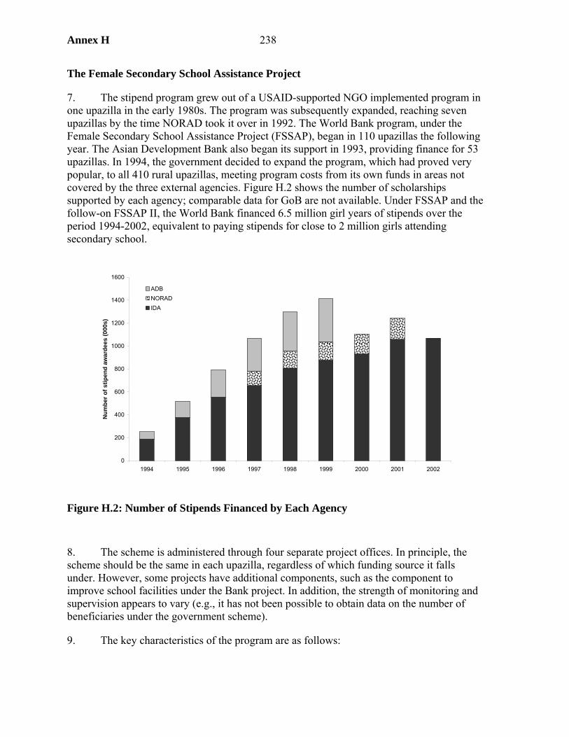
Annex H 238

0

200

400

600

800

1000

1200

1400

1600

1994 1995 1996 1997 1998 1999 2000 2001 2002

Num

ber o

f stip

end

awar

dees

(000

s)

ADBNORADIDA

The Female Secondary School Assistance Project

7. The stipend program grew out of a USAID-supported NGO implemented program in one upazilla in the early 1980s. The program was subsequently expanded, reaching seven upazillas by the time NORAD took it over in 1992. The World Bank program, under the Female Secondary School Assistance Project (FSSAP), began in 110 upazillas the following year. The Asian Development Bank also began its support in 1993, providing finance for 53 upazillas. In 1994, the government decided to expand the program, which had proved very popular, to all 410 rural upazillas, meeting program costs from its own funds in areas not covered by the three external agencies. Figure H.2 shows the number of scholarships supported by each agency; comparable data for GoB are not available. Under FSSAP and the follow-on FSSAP II, the World Bank financed 6.5 million girl years of stipends over the period 1994-2002, equivalent to paying stipends for close to 2 million girls attending secondary school.

Figure H.2: Number of Stipends Financed by Each Agency 8. The scheme is administered through four separate project offices. In principle, the scheme should be the same in each upazilla, regardless of which funding source it falls under. However, some projects have additional components, such as the component to improve school facilities under the Bank project. In addition, the strength of monitoring and supervision appears to vary (e.g., it has not been possible to obtain data on the number of beneficiaries under the government scheme).

9. The key characteristics of the program are as follows:

239 Annex H

• The stipend is paid to all girls attending rural secondary schools which are enrolled in the program. The stipend is paid into a bank account in the girl’s name (where there are no local branches of the bank administering the scheme, it opens booths for this purpose). Tuition is paid directly to the school.

• The school has to certify that the girl attends school on at least 75 percent of school days, and that she is attaining passing grades (45 percent).

• The girl must remain unmarried.

10. The stipend, which increases by grade, is intended to cover a proportion of the direct costs of the girl’s education. It does not fully cover these costs, especially as it has remained the same in nominal terms since the scheme began.

11. The stipend has not changed in nominal terms over the lifetime of the project. Including the two exam payments of Tk 250, the total amount paid per girl during the course of her education is Tk 3,914 (using a simple average of government and nongovernmental tuition fees, Table H.2). At the 2000 exchange rate this amount equals US$75.30. Allowing an administrative markup of 20 percent,1 brings the cost per girl to US$90.40.

Table H.2: Stipend Payments under FSSAP

Grade Stipend (monthly)

Tuition (govt.)

Tuition (non-govt.) SSC exam fee

6 25 10 15 .. 7 30 12 15 .. 8 35 12 15 .. 9 60 15 20 250 10 60 15 20 250

Source: FSSAP ICR : 31. 12. An alternative way to arrive at the estimated cost per girl is to divide the cost of the World Bank FSSAP, Tk 4,518.2 million, by the number of girl years supported by the project (4.904 million), which gives a figure of Tk 920 per girl year, which is US$17.8 per girl year. Since the stipend runs for five years, this multiplies to US$88.60 per girl. Hence, both approaches result in an estimate of US$90 in stipend payments per girl during the course of her secondary education.

13. Female secondary enrollment has grown rapidly since the stipend has been introduced, at a rate of over 10 percent a year since 1993. However, the important question is the extent to which this expansion in female enrollments has been the result of the stipend program. An upper limit of the program impact is given by the whole rise in female secondary enrollments in rural areas since 1993. But this figure would clearly be an overestimate. Enrollments had anyhow been rising before the introduction of stipends. The OED PPAR of FSSAP suggested that other factors may have been more important than the stipend, notably (1) the increasing number of girls completing primary school, which meant that girls enrollment at secondary level grew much more rapidly than it did for boys over the decade before the program, and (2) free tuition for girls in grades 6-8, which was established 1. The ratio of the total budget for FSSAP to the stipend component is 1.20, giving an overhead of 20 percent.

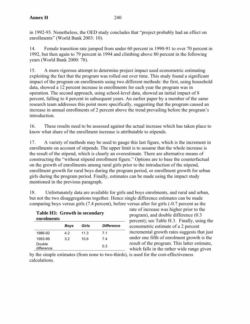
Annex H 240

in 1992-93. Nonetheless, the OED study concludes that “project probably had an effect on enrollments” (World Bank 2003: 10).

14. Female transition rate jumped from under 60 percent in 1990-91 to over 70 percent in 1992, but then again to 79 percent in 1994 and climbing above 80 percent in the following years (World Bank 2000: 78).

15. A more rigorous attempt to determine project impact used econometric estimating exploiting the fact that the program was rolled out over time. This study found a significant impact of the program on enrollments using two different methods: the first, using household data, showed a 12 percent increase in enrollments for each year the program was in operation. The second approach, using school-level data, showed an initial impact of 8 percent, falling to 4 percent in subsequent years. An earlier paper by a member of the same research team addresses this point more specifically, suggesting that the program caused an increase in annual enrollments of 2 percent above the trend prevailing before the program’s introduction.

16. These results need to be assessed against the actual increase which has taken place to know what share of the enrollment increase is attributable to stipends.

17. A variety of methods may be used to gauge this last figure, which is the increment in enrollments on account of stipends. The upper limit is to assume that the whole increase is the result of the stipend, which is clearly an overestimate. There are alternative means of constructing the “without stipend enrollment figure.” Options are to base the counterfactual on the growth of enrollments among rural girls prior to the introduction of the stipend, enrollment growth for rural boys during the program period, or enrollment growth for urban girls during the program period. Finally, estimates can be made using the impact study mentioned in the previous paragraph.

18. Unfortunately data are available for girls and boys enrolments, and rural and urban, but not the two disaggregations together. Hence single difference estimates can be made comparing boys versus girls (7.4 percent), before versus after for girls (-0.7 percent as the

rate of increase was higher prior to the program), and double difference (0.3 percent); see Table H.3. Finally, using the econometric estimate of a 2 percent incremental growth rates suggests that just under one fifth of enrolment growth is the result of the program. This latter estimate, which falls in the rather wide range given

by the simple estimates (from none to two-thirds), is used for the cost-effectiveness calculations.

Table H3: Growth in secondary enrolments Boys Girls Difference

1986-92 4.2 11.3 7.1 1993-99 3.2 10.6 7.4 Double difference 0.3

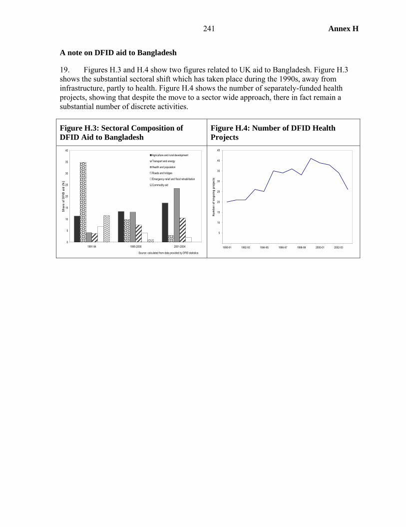
241 Annex H

A note on DFID aid to Bangladesh

19. Figures H.3 and H.4 show two figures related to UK aid to Bangladesh. Figure H.3 shows the substantial sectoral shift which has taken place during the 1990s, away from infrastructure, partly to health. Figure H.4 shows the number of separately-funded health projects, showing that despite the move to a sector wide approach, there in fact remain a substantial number of discrete activities.

Figure H.3: Sectoral Composition of DFID Aid to Bangladesh

Figure H.4: Number of DFID Health Projects

0

5

10

15

20

25

30

35

40

1991-94 1995-2000 2001-2004

Shar

e of

DFI

D a

id (%

)

Agriculture and rural development

Transport and energy

Health and population

Roads and bridges

Emergency relief and flood rehabilitation

Commodity aid

Source: calculated from data provided by DFID statistics

5

10

15

20

25

30

35

40

45

1990-91 1992-93 1994-95 1996-97 1998-99 2000-01 2002-03

Num

ber o

f ong

oing

pro

ject

s

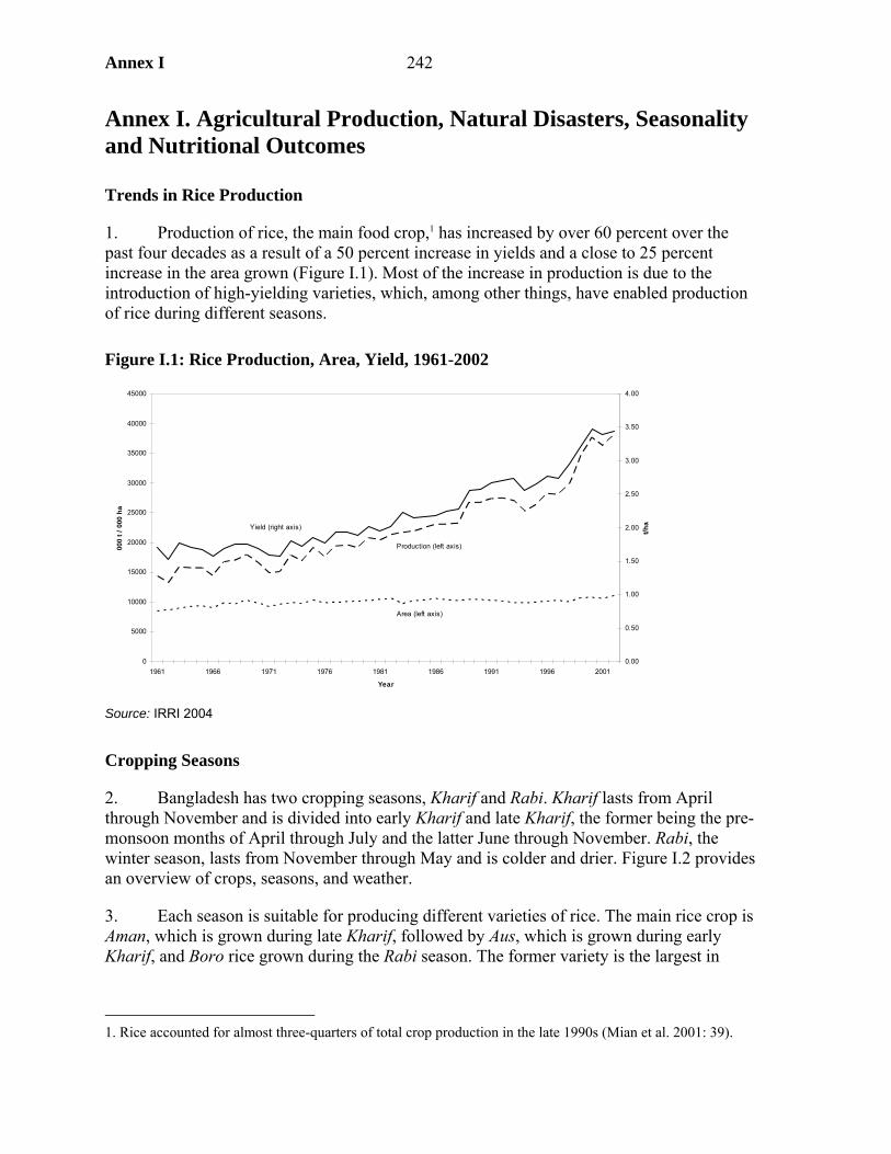
Annex I 242

Annex I. Agricultural Production, Natural Disasters, Seasonality and Nutritional Outcomes

Trends in Rice Production

1. Production of rice, the main food crop,1 has increased by over 60 percent over the past four decades as a result of a 50 percent increase in yields and a close to 25 percent increase in the area grown (Figure I.1). Most of the increase in production is due to the introduction of high-yielding varieties, which, among other things, have enabled production of rice during different seasons.

Figure I.1: Rice Production, Area, Yield, 1961-2002

Source: IRRI 2004

Cropping Seasons

2. Bangladesh has two cropping seasons, Kharif and Rabi. Kharif lasts from April through November and is divided into early Kharif and late Kharif, the former being the pre-monsoon months of April through July and the latter June through November. Rabi, the winter season, lasts from November through May and is colder and drier. Figure I.2 provides an overview of crops, seasons, and weather.

3. Each season is suitable for producing different varieties of rice. The main rice crop is Aman, which is grown during late Kharif, followed by Aus, which is grown during early Kharif, and Boro rice grown during the Rabi season. The former variety is the largest in

1. Rice accounted for almost three-quarters of total crop production in the late 1990s (Mian et al. 2001: 39).

0

5000

10000

15000

20000

25000

30000

35000

40000

45000

1961 1966 1971 1976 1981 1986 1991 1996 2001

Year

000

t / 0

00 h

a

0.00

0.50

1.00

1.50

2.00

2.50

3.00

3.50

4.00

t/ha

Area (left axis)

Production (left axis)

Yield (right axis)

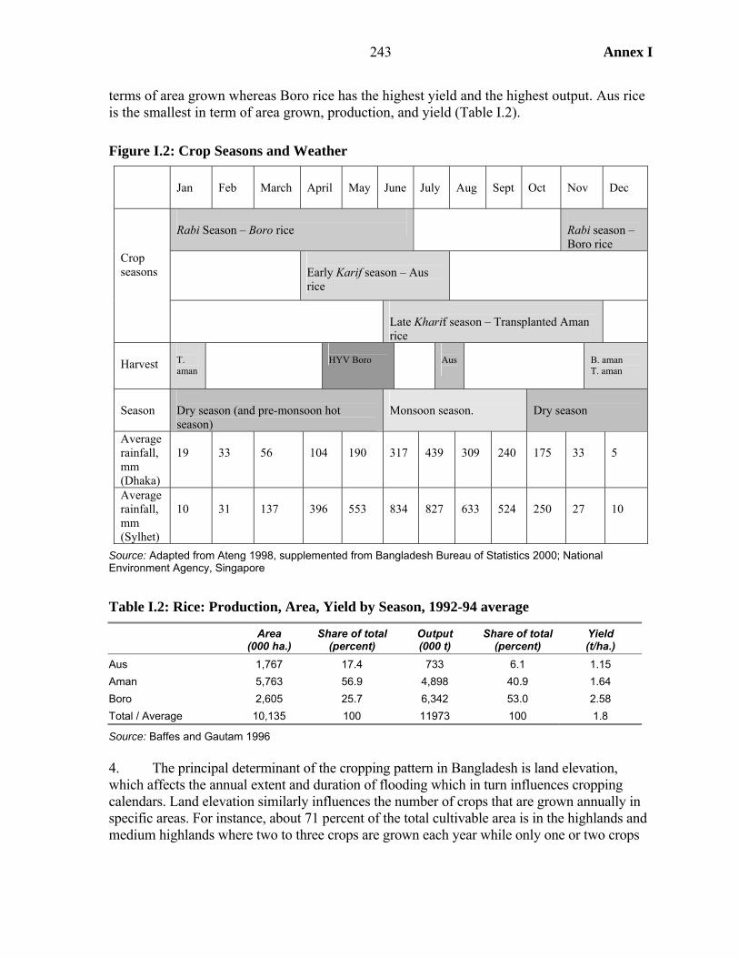
243 Annex I

terms of area grown whereas Boro rice has the highest yield and the highest output. Aus rice is the smallest in term of area grown, production, and yield (Table I.2).

Figure I.2: Crop Seasons and Weather

Jan

Feb

March

April

May

June

July

Aug

Sept

Oct

Nov

Dec

Rabi Season – Boro rice

Rabi season – Boro rice

Early Karif season – Aus rice

Crop seasons

Late Kharif season – Transplanted Aman rice

Harvest

T. aman

HYV Boro

Aus

B. aman T. aman

Season

Dry season (and pre-monsoon hot season)

Monsoon season.

Dry season

Average rainfall, mm (Dhaka)

19

33

56

104

190

317

439

309

240

175

33

5

Average rainfall, mm (Sylhet)

10

31

137

396

553

834

827

633

524

250

27

10

Source: Adapted from Ateng 1998, supplemented from Bangladesh Bureau of Statistics 2000; National Environment Agency, Singapore

Table I.2: Rice: Production, Area, Yield by Season, 1992-94 average

Area

(000 ha.) Share of total

(percent) Output (000 t)

Share of total (percent)

Yield (t/ha.)

Aus 1,767 17.4 733 6.1 1.15 Aman 5,763 56.9 4,898 40.9 1.64 Boro 2,605 25.7 6,342 53.0 2.58 Total / Average 10,135 100 11973 100 1.8

Source: Baffes and Gautam 1996 4. The principal determinant of the cropping pattern in Bangladesh is land elevation, which affects the annual extent and duration of flooding which in turn influences cropping calendars. Land elevation similarly influences the number of crops that are grown annually in specific areas. For instance, about 71 percent of the total cultivable area is in the highlands and medium highlands where two to three crops are grown each year while only one or two crops

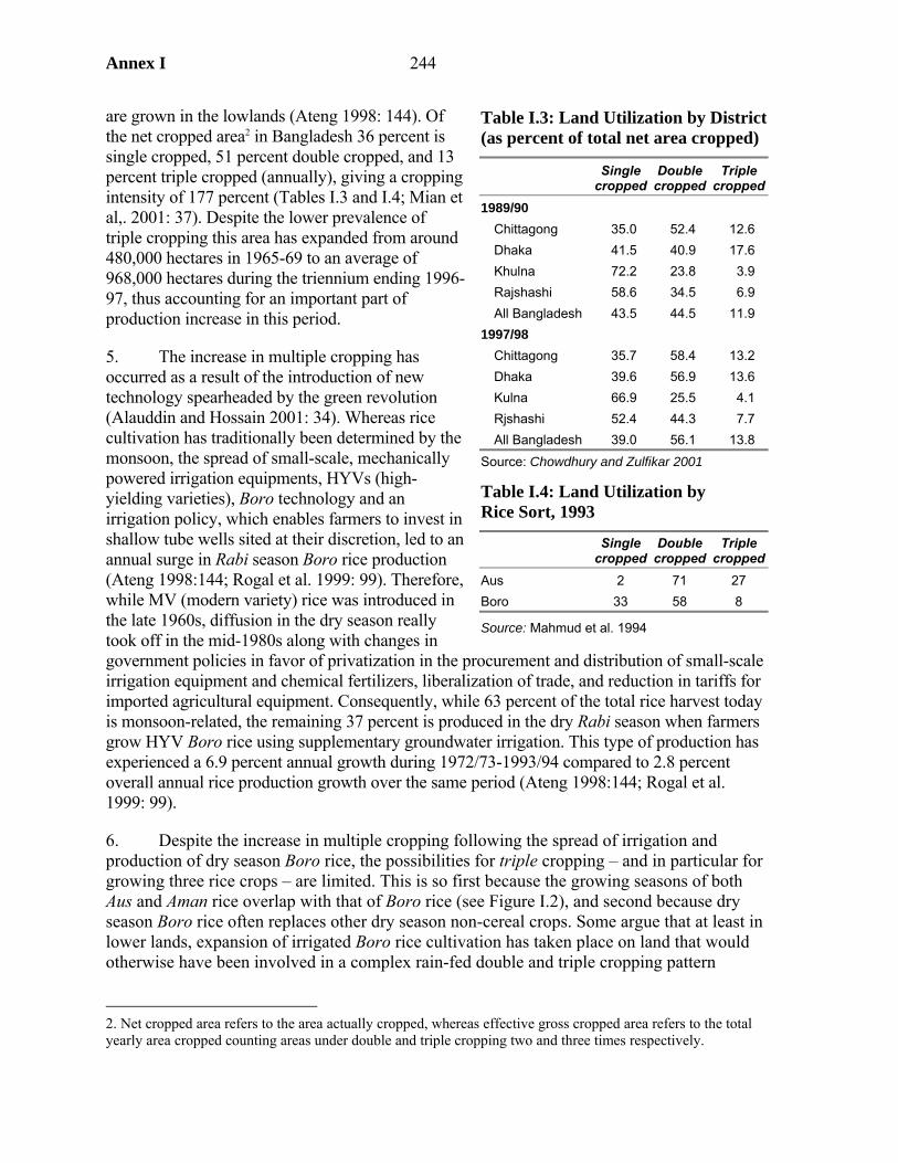
Annex I 244

are grown in the lowlands (Ateng 1998: 144). Of the net cropped area2 in Bangladesh 36 percent is single cropped, 51 percent double cropped, and 13 percent triple cropped (annually), giving a cropping intensity of 177 percent (Tables I.3 and I.4; Mian et al,. 2001: 37). Despite the lower prevalence of triple cropping this area has expanded from around 480,000 hectares in 1965-69 to an average of 968,000 hectares during the triennium ending 1996-97, thus accounting for an important part of production increase in this period.

5. The increase in multiple cropping has occurred as a result of the introduction of new technology spearheaded by the green revolution (Alauddin and Hossain 2001: 34). Whereas rice cultivation has traditionally been determined by the monsoon, the spread of small-scale, mechanically powered irrigation equipments, HYVs (high-yielding varieties), Boro technology and an irrigation policy, which enables farmers to invest in shallow tube wells sited at their discretion, led to an annual surge in Rabi season Boro rice production (Ateng 1998:144; Rogal et al. 1999: 99). Therefore, while MV (modern variety) rice was introduced in the late 1960s, diffusion in the dry season really took off in the mid-1980s along with changes in government policies in favor of privatization in the procurement and distribution of small-scale irrigation equipment and chemical fertilizers, liberalization of trade, and reduction in tariffs for imported agricultural equipment. Consequently, while 63 percent of the total rice harvest today is monsoon-related, the remaining 37 percent is produced in the dry Rabi season when farmers grow HYV Boro rice using supplementary groundwater irrigation. This type of production has experienced a 6.9 percent annual growth during 1972/73-1993/94 compared to 2.8 percent overall annual rice production growth over the same period (Ateng 1998:144; Rogal et al. 1999: 99).

6. Despite the increase in multiple cropping following the spread of irrigation and production of dry season Boro rice, the possibilities for triple cropping – and in particular for growing three rice crops – are limited. This is so first because the growing seasons of both Aus and Aman rice overlap with that of Boro rice (see Figure I.2), and second because dry season Boro rice often replaces other dry season non-cereal crops. Some argue that at least in lower lands, expansion of irrigated Boro rice cultivation has taken place on land that would otherwise have been involved in a complex rain-fed double and triple cropping pattern

2. Net cropped area refers to the area actually cropped, whereas effective gross cropped area refers to the total yearly area cropped counting areas under double and triple cropping two and three times respectively.

Table I.3: Land Utilization by District (as percent of total net area cropped)

Single

cropped Double

cropped Triple

cropped1989/90

Chittagong 35.0 52.4 12.6 Dhaka 41.5 40.9 17.6 Khulna 72.2 23.8 3.9 Rajshashi 58.6 34.5 6.9 All Bangladesh 43.5 44.5 11.9

1997/98 Chittagong 35.7 58.4 13.2 Dhaka 39.6 56.9 13.6 Kulna 66.9 25.5 4.1 Rjshashi 52.4 44.3 7.7 All Bangladesh 39.0 56.1 13.8

Source: Chowdhury and Zulfikar 2001

Table I.4: Land Utilization by Rice Sort, 1993

Single

cropped Double

cropped Triple

croppedAus 2 71 27 Boro 33 58 8

Source: Mahmud et al. 1994

245 Annex I

involving broadcast Aus,3 broadcast Aman, and a range of other winter crops. Since most non-cereal crops are grown on non-irrigated land and compete for land in the dry season these crops are thus liable to be replaced with the expansion of irrigation (Jaim 1984: 36; Ateng 1998: 146-8). This argument is supported by looking at the proportion of Aus and Boro rice cropped areas under triple cropping. Ten percent of MV Aus cropped area is under rice-only triple cropping and 17 percent is under rice and other triple cropping, while 7 percent of Boro rice is under rice-only triple cropping, and only 1 percent under rice and other triple cropping (Mahmud et al. 1994: 30).

7. Because Aman rice is the largest crop in terms of area grown, and makes up close to 60 percent of total rice grown area (Table I.4), November-December remains the main harvest season with the widest food availability. May-June, when Boro rice is harvested, is the second most important harvest.

Aggregate Output, Disasters, and Daily Energy Supply

8. As rice is the major agricultural crop, the trend in daily energy supply per capita closely follows rice production, notably the upsurge in the late 1990s (Figure I.3). The figure also shows the major disasters during this period, which for the most part seem to have not had a large an impact an aggregate production, which is not to say there may not have been regional effects. Daily energy supply also appears not to suffer during disasters (Table I.5), sometimes even increasing, presumably reflecting relief food aid.

Seasonality and Nutrition

9. Cropping patterns determine harvest seasons, which in turn influence work, employment, food intake, and nutrition in rural areas. As the largest crop, Aman is the most important in this respect. Demand for agricultural labor is highest during the Aman harvest, while opportunities for employment are also enhanced during production and harvest of Boro and Aus – for instance during the months of January and March when the transplantation of HYV Boro takes place (Pitt and Khandker 2002: 12). The introduction of new agricultural technology has made significant contribution to employment creation, rather than the reverse, especially HYV Boro rice (Alauddin and Tisdell 1998: 86-9).

3. Transplanted, broadcast, and deepwater rice are different varieties of rice, which exist within each rice sort. Each of these contains various subgroups.

Table I.5: Top 10 Disasters in Bangladesh by Number of People Affected

Disaster Date Affected (millions)

Flood 22 July 1987 73.0 Flood August 1988 73.0 Flood July 1974 38.0 Flood 20 June 2004 33.6 Flood May 1984 30.0 Drought 5 July 1983 20.0 Flood Jul 1968 15.9 Wind Storm 11 May 1965 15.6 Wind Storm 30 April 1991 15.4 Flood 8 July 1998 15.0

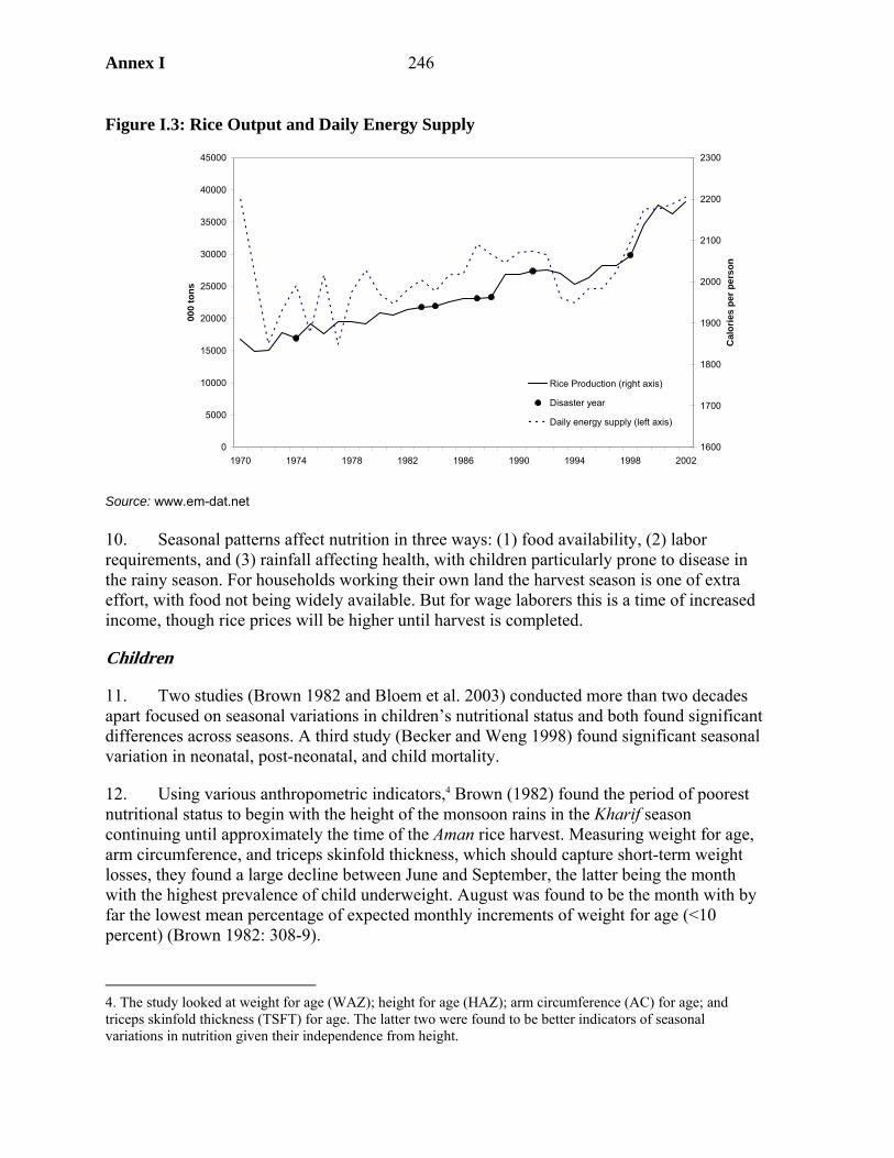
Annex I 246

0

5000

10000

15000

20000

25000

30000

35000

40000

45000

1970 1974 1978 1982 1986 1990 1994 1998 2002

000

tons

1600

1700

1800

1900

2000

2100

2200

2300

Cal

orie

s pe

r per

son

Rice Production (right axis)

Disaster year

Daily energy supply (left axis)

Figure I.3: Rice Output and Daily Energy Supply

Source: www.em-dat.net 10. Seasonal patterns affect nutrition in three ways: (1) food availability, (2) labor requirements, and (3) rainfall affecting health, with children particularly prone to disease in the rainy season. For households working their own land the harvest season is one of extra effort, with food not being widely available. But for wage laborers this is a time of increased income, though rice prices will be higher until harvest is completed.

Children

11. Two studies (Brown 1982 and Bloem et al. 2003) conducted more than two decades apart focused on seasonal variations in children’s nutritional status and both found significant differences across seasons. A third study (Becker and Weng 1998) found significant seasonal variation in neonatal, post-neonatal, and child mortality.

12. Using various anthropometric indicators,4 Brown (1982) found the period of poorest nutritional status to begin with the height of the monsoon rains in the Kharif season continuing until approximately the time of the Aman rice harvest. Measuring weight for age, arm circumference, and triceps skinfold thickness, which should capture short-term weight losses, they found a large decline between June and September, the latter being the month with the highest prevalence of child underweight. August was found to be the month with by far the lowest mean percentage of expected monthly increments of weight for age (<10 percent) (Brown 1982: 308-9).

4. The study looked at weight for age (WAZ); height for age (HAZ); arm circumference (AC) for age; and triceps skinfold thickness (TSFT) for age. The latter two were found to be better indicators of seasonal variations in nutrition given their independence from height.

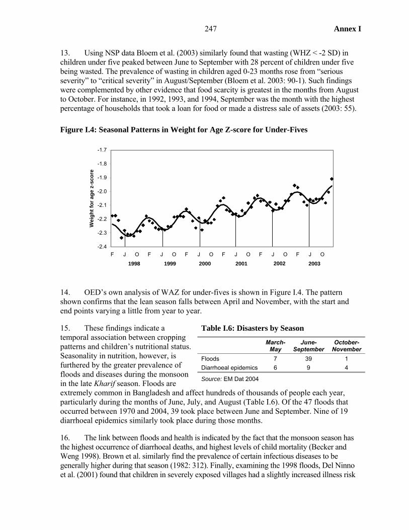
247 Annex I

13. Using NSP data Bloem et al. (2003) similarly found that wasting (WHZ < -2 SD) in children under five peaked between June to September with 28 percent of children under five being wasted. The prevalence of wasting in children aged 0-23 months rose from “serious severity” to “critical severity” in August/September (Bloem et al. 2003: 90-1). Such findings were complemented by other evidence that food scarcity is greatest in the months from August to October. For instance, in 1992, 1993, and 1994, September was the month with the highest percentage of households that took a loan for food or made a distress sale of assets (2003: 55).

Figure I.4: Seasonal Patterns in Weight for Age Z-score for Under-Fives

14. OED’s own analysis of WAZ for under-fives is shown in Figure I.4. The pattern shown confirms that the lean season falls between April and November, with the start and end points varying a little from year to year.

15. These findings indicate a temporal association between cropping patterns and children’s nutritional status. Seasonality in nutrition, however, is furthered by the greater prevalence of floods and diseases during the monsoon in the late Kharif season. Floods are extremely common in Bangladesh and affect hundreds of thousands of people each year, particularly during the months of June, July, and August (Table I.6). Of the 47 floods that occurred between 1970 and 2004, 39 took place between June and September. Nine of 19 diarrhoeal epidemics similarly took place during those months.

16. The link between floods and health is indicated by the fact that the monsoon season has the highest occurrence of diarrhoeal deaths, and highest levels of child mortality (Becker and Weng 1998). Brown et al. similarly find the prevalence of certain infectious diseases to be generally higher during that season (1982: 312). Finally, examining the 1998 floods, Del Ninno et al. (2001) found that children in severely exposed villages had a slightly increased illness risk

Table I.6: Disasters by Season

March-

May June-

September October-

November Floods 7 39 1 Diarrhoeal epidemics 6 9 4

Source: EM Dat 2004

-2.4

-2.3

-2.2

-2.1

-2.0

-1.9

-1.8

-1.7

F J O F J O F J O F J O F J O F J O

Wei

ght f

or a

ge z

-sco

re

1998 1999 2000 2001 2002 2003

Annex I 248

and for those in very severely exposed villages the risk more than trebled; the incidence of fever rose by 55 percent and that of diarrhea by 25 percent, which will affect nutritional outcomes.

Women

17. OED analysis of the NSP data shows that seasonal variations in underweight are not the same for children and women. Whereas children’s weight for age is lowest during the monsoon in June-July and the “hungry months” preceding the Aman harvest, and highest during November and December, women’s Body Mass Index (BMI) peaks in August-September and is lowest in December. Maternal calorie deficiency (CED) is most severe in December and January and least so in August/September (although seasonal variation is not found to be very large: 43 percent in December/January versus 36 percent in August/September) (Bloem et al. 2003).

18. Such seasonal variations in female malnourishment are most likely explained by the significant increase in women’s workload. A qualitative study of women’s schedules and time constraints found them to vary according to the agricultural season as harvest seasons and rice processing significantly affects time use Levinson et al. (2002). The busiest seasons for women are the crop harvest seasons from mid-April to mid-June and from mid-November to mid-January. The rice harvest months of mid-April to mid-May and mid-November to mid-December (Figure I.2) are the times when women generally prepare the least number of meals because they lack time to do so. Most women in the study said that they managed to complete their tasks only by sleeping, resting, and bathing less. Finally, the study found that women considered time a more serious problem with respect to self-care than to childcare. For example, they regarded eating more food during pregnancy as difficult given their time constraints, whereas providing complementary food to their children or giving them more than three meals a day was given higher priority.

Figure I.4: Seasonal Patterns of Women’s Body Mass Index

18.4

18.6

18.8

19

19.2

19.4

19.6

19.8

F J O F J O F J O F J O

Bod

y m

ass

inde

x

2000 20032001 2002

Annex J

249

Annex J. Approach Paper

Background and rationale

1. Two of the eight Millennium Development Goals (MDGs) refer to maternal and child health, and child malnutrition is a Goal 1 indicator. The results-based rationale of the MDGs requires understanding the main drivers behind changes in MDG indicators: what can government policy and interventions, assisted by external partners, do to accelerate the pace of improvement and so secure the achievement of the goals?

TABLE J1 MCH-RELATED MILLENNIUM DEVELOPMENT GOALS

(a) Goal Target Indicators

Goal 1: Eradicate extreme poverty and hunger

Target 2: Halve, between 1990 and 2015, the proportion of people who suffer from hunger

Prevalence of underweight children (under five years of age)

Proportion of population below minimum level of dietary energy consumption

Goal 4: Reduce child mortality

Target 5: Reduce by two-thirds, between 1990 and 2015, the under-five mortality rate

Under-five mortality rate

Infant mortality rate Proportion of one-year-old children immunized against measles

Goal 5: Improve maternal health

Target 6: Reduce by three-quarters, between 1990 and 2015, the maternal mortality ratio

Maternal mortality ratio

Proportion of births attended by skilled health personnel

2. The impact studies being undertaken by OED, under the OED-DFID partnership agreement, seek to address this issue, focusing in this case on maternal and child health (MCH) outcomes in Bangladesh. The study will build upon the methods developed during the first impact evaluation carried out under the partnership agreement which analyzed the impact of the external support to basic education in Ghana from the Bank, DFID and USAID.1 This approach is based on the combination of rigorous statistical analysis of outcomes with contextual analysis based on qualitative material. As a joint evaluation under the partnership agreement interventions supported by both the Bank and DFID will be included in the study. 3. The focus of the study will not, however, be restricted to interventions in health, nutrition and population (HNP), since MCH outcomes are also affected by activities in other

1. Books, Buildings and Learning Outcomes: an impact evaluation of World Bank support to basic education in Ghana, OED, January 2004.

Annex J

250

sectors. In the words of the 2004 World Development Report “the determinants of supply and demand operate through many channels” (WDR, 2004, p.27). OED’s own review of the MDGs similarly stressed the need for multi-sectoral strategies to achieve single-sector targets.2 DFID’s target strategy paper, Better Health for Poor People, states that, “good health is determined by many factors, the most important of which is reaching and sustaining a reasonable level of income and consumption. Female education, clean water and, most importantly, sanitation have an important and well documented impact on (in particular) child survival. Female empowerment is vital to enable women and families access to health care” (DFID, 2000: 9). 4. Bangladesh has been chosen for a number of reasons. It is a country which has made impressive progress in reducing both under five mortality and fertility. External partners, including both the World Bank and DFID, have been active in supporting large-scale interventions with specific objectives to improve maternal and child health. Improved access to health services especially for poor women and children was included under the first objective in DFID’s country strategy for Bangladesh formulated in 1998. During recent years external interventions in the population and health sectors have been coordinated under a sector program in which both DFID and the Bank have been active partners. Finally, there are a substantial number of large data sets appropriate for the analysis.

The Bangladesh context

5. Bangladesh presents a mixed picture with respect to MCH indicators. Over the 1990s infant and child mortality have been halved: unlike most countries, Bangladesh has a sufficient rate of progress to meet the MDG target of a two-thirds reduction by 2015. Fertility also fell rapidly from the 1980s, although there are fears in some quarters that the indicator has now reached a plateau. However, despite low levels of fertility, maternal mortality is high: at between 320 and 400 per 100,000 live births it is greater than that in both India and Pakistan and six times that in Sri Lanka. Intermediate indicators show a similar discrepancy. Immunization rates have grown rapidly in Bangladesh and are today notably higher than those in neighboring countries. But only 13 per cent of births are delivered by skilled birth attendants, compared to close to half in India. 6. The study will focus on interventions from several sectors. The chosen interventions will be those supported by DFID and the World Bank, and other donors subject to the required information being available. Amongst these sectors will be health and population, which has accounted for 17 percent of DFID aid to Bangladesh in recent years (Annex 1b) and, together with nutrition, 7 percent of Bank lending (Annex 1a). As described below, the other sectors are to be identified based on an analysis of the determinants of MCH outcomes. 7. On the Bank’s part there have been five Health and Population projects in Bangladesh: I (1974-80), II( 1979-86), III (1986-92), IV (1992-98) and the Health and

2. 02 Annual Review of Development Effectiveness - Achieving Development Outcomes: The Millennium Challenge, OED, report no. 25159.

Annex J

251

Population Program Project (ongoing since 1998), the last three of which have been co-financed by DFID. In addition there is the Bangladesh Integrated Nutrition Project (BINP, 1995-02), which is being followed up by the National Nutrition Project (NNP, ongoing since 2000). All these projects have specific objectives related to maternal and child health. The study will include, amongst other interventions, PHP III, IV and HPSP, and BINP. 8. DFID’s support for HPSP has been principally to Strengthen Health and Population for the Less Advantaged (SHAPLA), through two mechanisms: (i) time slice financing of the HPSP budget, and (ii) project support focused in key areas of HPSP to strengthen government’s implementation capacity and to minimize risk. Both Bank and DFID financing to the population and health sector has had several components which will be assessed separately for their inclusion in the study. Other donor interventions to be included in the study will be provisionally identified at the design stage.

9. In line with the multi-sectoral philosophy of the MDGs (i.e. the notion that the relevant interventions for each outcome are in a range of sectors) the study will consider interventions from outside the HNP sector. For example, income-generation activities will also positively affect MCH outcomes, as will improved water supply and better education. The analysis of other sectors will be carried out through a two stage approach described below. Evaluation questions

10. The evaluation questions to be addressed are:

(a) What is happening to maternal and child health indicators (including nutrition

and fertility) in Bangladesh? Are the poor sharing in the progress which is being made?

(b) What have been the main determinants of MCH outcomes in Bangladesh over

this period, and which of these have accounted for substantial changes? (c) What have been the primary drivers of changes in the determinants of MCH

outcomes since the mid-80s?3

(d) What have been the range of government and externally-supported interventions which may have affected the changes in the determinants of MCH outcomes?

(e) To the extent that interventions have brought about positive impacts, have they

done so in a cost effective manner?

3. Determinants are the variables entering the multiple regression analysis, such as mother’s education, and drivers the policies and programs which drive changes in these determinants (e.g. policy on school fees, and female scholarships).

Annex J

252

Evaluation approach and data requirements

11. The analytical framework for the evaluation is provided by the combination of two widely-adopted frameworks - UNICEF’s conceptual framework of the causes of malnutrition4 and the Mosley-Chen analytical framework of child survival5 - together with the insights from household models of the demand for health used in economics.6 The first two frameworks have the same outcome variables (malnutrition and mortality) and essentially the same structure, in which the basic causes come from a country’s socio-economic and institutional conditions, but these are mediated through a number of proximate causes observed at the community, household and individual levels. Maternal health is both a determinant of child welfare outcomes and an outcome in its own right. Economic models also highlight the importance of behavioral factors (“tastes and preferences”) in affecting demand for health services. 12. The framework identifies the determinants of MCH outcomes in broad terms thus providing a theoretical basis for the selection of variables for modeling these outcomes. These determinants have been examined more closely in a meta-analysis of infant and child mortality and nutrition, prepared as a background paper for this study (see appendix 3 for a summary of determinants identified by this analysis). 13. The adoption of a theory-based evaluation approach will direct attention to further assumptions contained in project design. For example, since health and nutrition interventions attempt to bring about behavior change they are partly built on the assumption of irrational beliefs regarding health and nutrition practices. But the data show some discrepancies between knowledge and practices, suggesting that projects may change knowledge but not practices. The most recent progress report for Bangladesh’s Health and Population Sector Program notes scant improvement in service use. The study will use both quantitative and qualitative methods to analyze issues such as patterns of service use and the rationale for various health and nutritional practices. 14. The determinants given in a regression model of MCH outcomes are not usually direct measures of policies or programs. The task for an impact evaluation is to link outputs from policies and programs with the determinants and hence to the final outcomes. This study will examine the link between MCH outcomes and DFID and Bank-supported interventions, together with those of other donors where possible, through a two stage approach. A regression-based decomposition analysis of the determinants of MCH outcomes will be used to identify which factors have been most important in changing outcomes in

4. UNICEF (1990) Strategy for Improved Nutrition of Children and Women in Developing Countries. New York: UNICEF. 5. W. Henry Mosley and Lincoln C. Chen (1984) “An analytical framework for the study of child survival in developing countries” Population Development Review Vol. 10 Supplement: Child Survival: strategies for research, 25-45. 6. For example, JM Currie ‘Child Health in Developing Countries’ in Culyer and Newhouse JP (eds). Handbook of Health Economics Amsterdam, Elevier Science BV, 2000.

Annex J

253

Bangladesh. This analysis will be used to identify which DFID, Bank and other interventions have directly supported improvements in MCH. The most important interventions will be selected for a more detailed analysis, to quantify the size and cost effectiveness of their impact. In addition to HNP, it is envisaged that two or three other sectors will be selected. The activities of the DFID and the Bank within these sectors will be examined, along with those of other donors where this proves feasible. The final selection of sectors will be an outcome of the first stage of the analysis. 15. An exception to this approach is BINP, which has an unusually rich evaluation dataset comprising a baseline, mid-term and endline surveys for both project sites and control communities. The data collected can be mapped onto the logic of the project, since intermediate process indicators relating to behavioral factors were included in the surveys in addition to outcome data and socio-economic status (SES) variables. These data are available to the study team together with the relevant documentation. Save the Children, who have been critical of the approach adopted by BINP, conducted their own survey in 2002 and these data will also be available to the study team. 16. Several other nationally-representative data sets exist for the relevant period. These are listed in Appendix 2. Surveys likely to be used are:

• Demographic Health Surveys: 1993/94, 1996/97 and 1999/2000 • Household income and expenditure surveys: 1991/92, 1995/96 and 2000 • Helen Keller International Nutritional Surveillance Project • Maternal mortality survey, 2003.

The first two of these surveys have been acquired for the study. The other two are not in the public domain, but can be analyzed through collaborative arrangements with their owners. 17. A review of existing material shall be undertaken during design to determine to what extent the analysis can rely on secondary data and to what extent commissioned studies are required. Relevant areas of analysis are: (a) trends in government expenditure,7 (b) facility and staffing survey, (c) demand for health services, and (d) behavioral changes related to health and nutritional practices. At least two of these issues will be examined through qualitative fieldwork using participatory analysis of such issues as perception of service quality and the rationale underling health and feeding practices.

Collaboration with other agencies

18. Collaboration shall be sought with relevant government officials or research institutions in Bangladesh. Commissioned studies from local organizations may include a 7. Public expenditure reviews are available from 1990, 1996, 1997 and 2003.

Annex J

254

component of capacity development through supported learning-by-doing. DFID staff in the Dhaka office shall facilitate the inclusion of DFID-supported interventions in the study and assist, together with Bank staff, liaison with other agencies as necessary.

Schedule and Task Management

19. The study will be undertaken in the following stages:

• Inception – comprising an inception field visit (February 2004), preparation of the

approach paper followed by preliminary fieldwork (April 2004) and development of the study design (April-May).

• Analysis first phase – analysis of household data sets of the determinants of

health, nutrition, and fertility outcomes. Background studies will be carried out in parallel. The results of these studies will be presented in Dhaka in late July or early August 2004 to feed into the discussions concerning future support. Identification of projects to be analyzed by the study will be carried out in this phase.

• Analysis second phase – collection and analysis of project-level data from DFID,

the Bank and other donors as possible.

• Report draft for OED management review to be ready by late October 2004, with submission to CODE of the final report targeted for January 2005.

20. The evaluation will be carried out by a team of OED staff and consultants with the assistance of Bangladeshi government officials, DFID staff under the Task Management of Howard White (OEDST). External peer reviewers will be appointed to review the proposed evaluation design and draft final report.

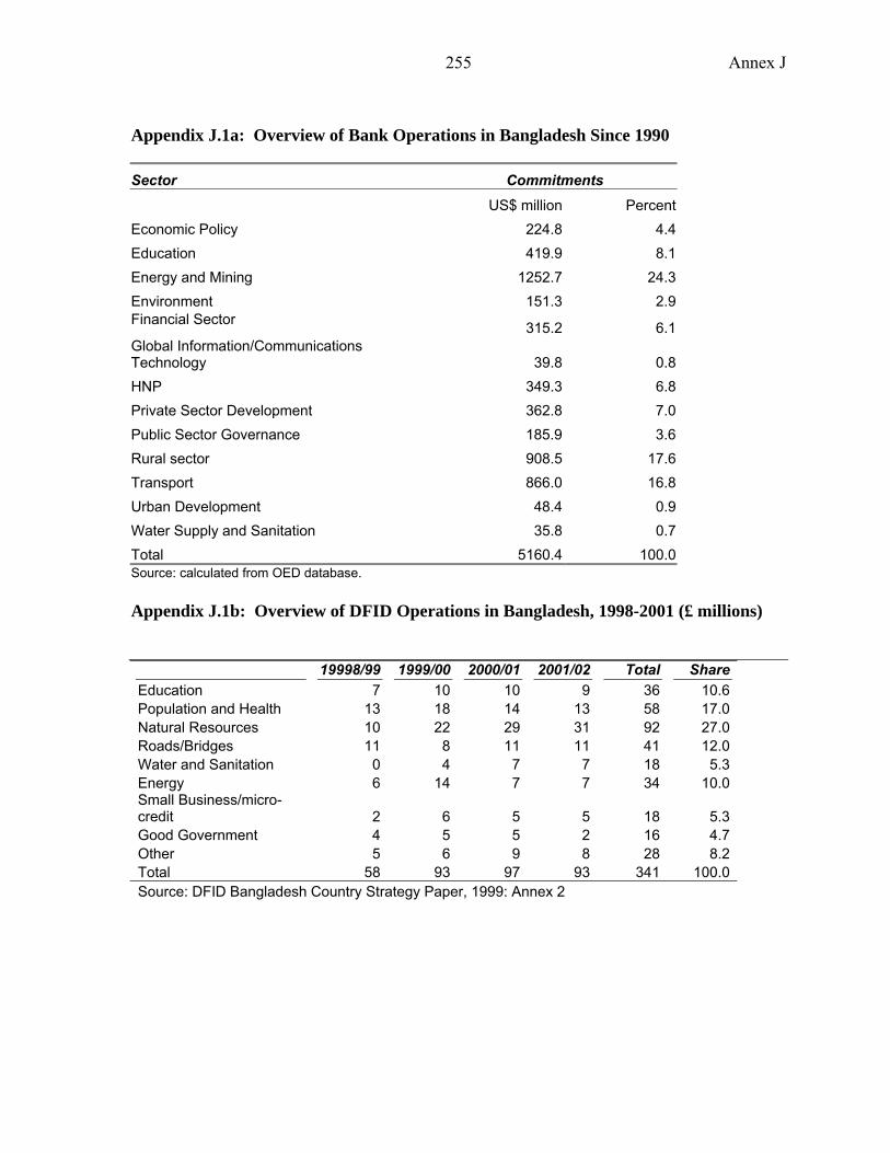
Annex J

255

Appendix J.1a: Overview of Bank Operations in Bangladesh Since 1990

Sector Commitments US$ million Percent Economic Policy 224.8 4.4 Education 419.9 8.1 Energy and Mining 1252.7 24.3 Environment 151.3 2.9 Financial Sector 315.2 6.1 Global Information/Communications Technology 39.8 0.8 HNP 349.3 6.8 Private Sector Development 362.8 7.0 Public Sector Governance 185.9 3.6 Rural sector 908.5 17.6 Transport 866.0 16.8 Urban Development 48.4 0.9 Water Supply and Sanitation 35.8 0.7 Total 5160.4 100.0 Source: calculated from OED database. Appendix J.1b: Overview of DFID Operations in Bangladesh, 1998-2001 (£ millions)

19998/99 1999/00 2000/01 2001/02 Total ShareEducation 7 10 10 9 36 10.6Population and Health 13 18 14 13 58 17.0Natural Resources 10 22 29 31 92 27.0Roads/Bridges 11 8 11 11 41 12.0Water and Sanitation 0 4 7 7 18 5.3Energy 6 14 7 7 34 10.0Small Business/micro-credit 2 6 5 5 18 5.3Good Government 4 5 5 2 16 4.7Other 5 6 9 8 28 8.2Total 58 93 97 93 341 100.0Source: DFID Bangladesh Country Strategy Paper, 1999: Annex 2

Annex J

256

Appendix J.2: List of Data Sets Survey (b) Content Availability

Demographic Health Survey

Child health and nutrition, child care practices, SES, comprehensive birth history. Includes some “women’s agency” questions.

Freely downloadable from Macro International website

BBS Health and demographic survey

As for DHS To determine if in Bank or not, otherwise purchase from BBS

BINP evaluation data set

Nutritional status, beliefs and practices, SES

Available in Bank and clearance has been obtained for use, awaiting data

SCF Bangladesh nutrition data set

Nutritional status and household characteristics

Was promised sometime ago, need to follow up

Household Income and Expenditure Survey

Standard LSMS type survey, but no anthropometrics. Only most recent has health module, but all have health expenditures

Most recent acquired, others available in Bank and being followed up

Health facility survey Not known yet Acquired

Helen Keller International National Nutrition Surveillance Survey

Nutritional status + SES. Every two months since 1990, with nationally representative sample since 1996. Content changes but a common core.

Proposed to contract HK to conduct analysis.

Vital registration sample survey (BBS)

Births, deaths and basic household and individual characteristics. Cause of death (quite aggregated).

Can be purchased from BBS. Possibly analyse in collaboration with BIDS

National Nutrition Survey (BBS)

Anthropometric measurement, SES. Can be purchased from BBS. Possibly analyse in collaboration with BIDS

UNICEF Multiple Indicators Cluster Survey

Range of social indicators, representative at district level.

Should be available from MICS website, for which clearance to download already obtained

UNICEF maternal health facility survey

Use, deliveries and materials availability

Statistics officer can perform analysis on request

Maternal Mortality Survey (USAID financed)

Maternal death (sisterhood and h/h based), SES

Not available but can influence form of analysis and receive results

Notes: Both BBS surveys began in the 1980s, but data may only be available for the last one or two rounds. All the above are household surveys. Some are supplemented by community-level data collection of variables such as facilities and prices. These are all national surveys; there are also more local data, notably those collected in Matlab thana which may also be utilized.

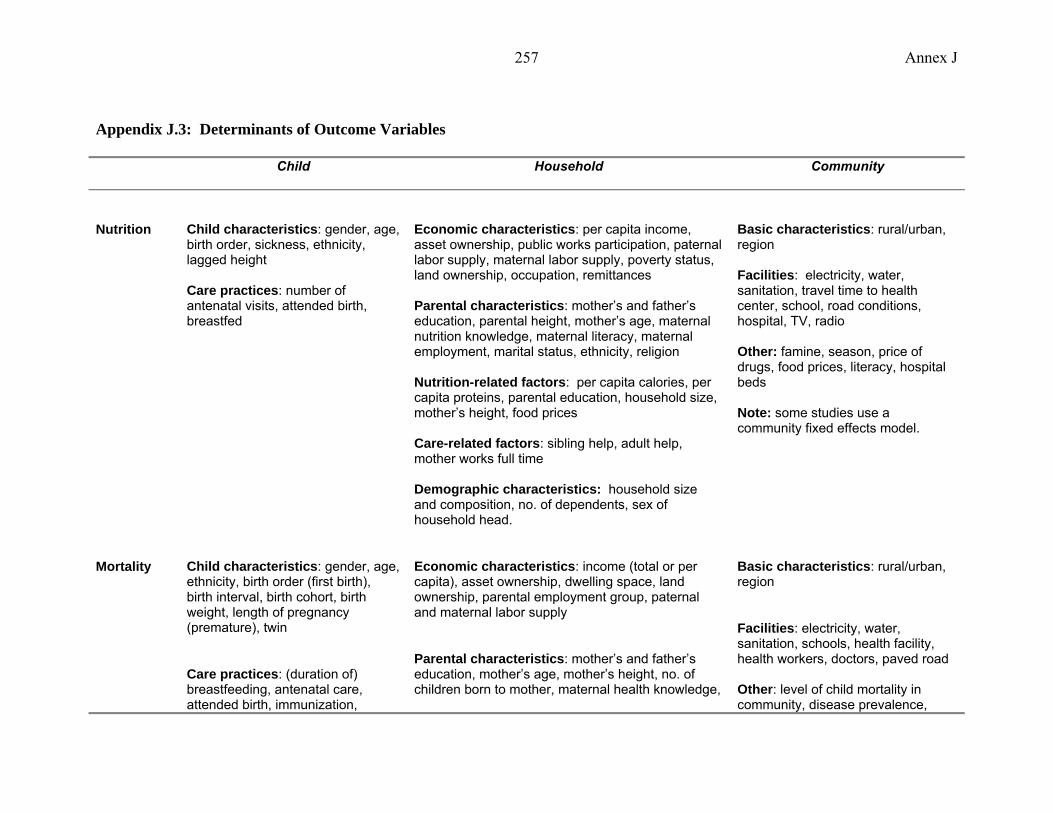
Annex J

257

Appendix J.3: Determinants of Outcome Variables Child Household Community

Nutrition Child characteristics: gender, age, birth order, sickness, ethnicity, lagged height Care practices: number of antenatal visits, attended birth, breastfed

Economic characteristics: per capita income, asset ownership, public works participation, paternal labor supply, maternal labor supply, poverty status, land ownership, occupation, remittances Parental characteristics: mother’s and father’s education, parental height, mother’s age, maternal nutrition knowledge, maternal literacy, maternal employment, marital status, ethnicity, religion Nutrition-related factors: per capita calories, per capita proteins, parental education, household size, mother’s height, food prices Care-related factors: sibling help, adult help, mother works full time Demographic characteristics: household size and composition, no. of dependents, sex of household head.

Basic characteristics: rural/urban, region Facilities: electricity, water, sanitation, travel time to health center, school, road conditions, hospital, TV, radio Other: famine, season, price of drugs, food prices, literacy, hospital beds Note: some studies use a community fixed effects model.

Mortality Child characteristics: gender, age, ethnicity, birth order (first birth), birth interval, birth cohort, birth weight, length of pregnancy (premature), twin

Care practices: (duration of) breastfeeding, antenatal care, attended birth, immunization,

Economic characteristics: income (total or per capita), asset ownership, dwelling space, land ownership, parental employment group, paternal and maternal labor supply

Parental characteristics: mother’s and father’s education, mother’s age, mother’s height, no. of children born to mother, maternal health knowledge,

Basic characteristics: rural/urban, region

Facilities: electricity, water, sanitation, schools, health facility, health workers, doctors, paved road Other: level of child mortality in community, disease prevalence,

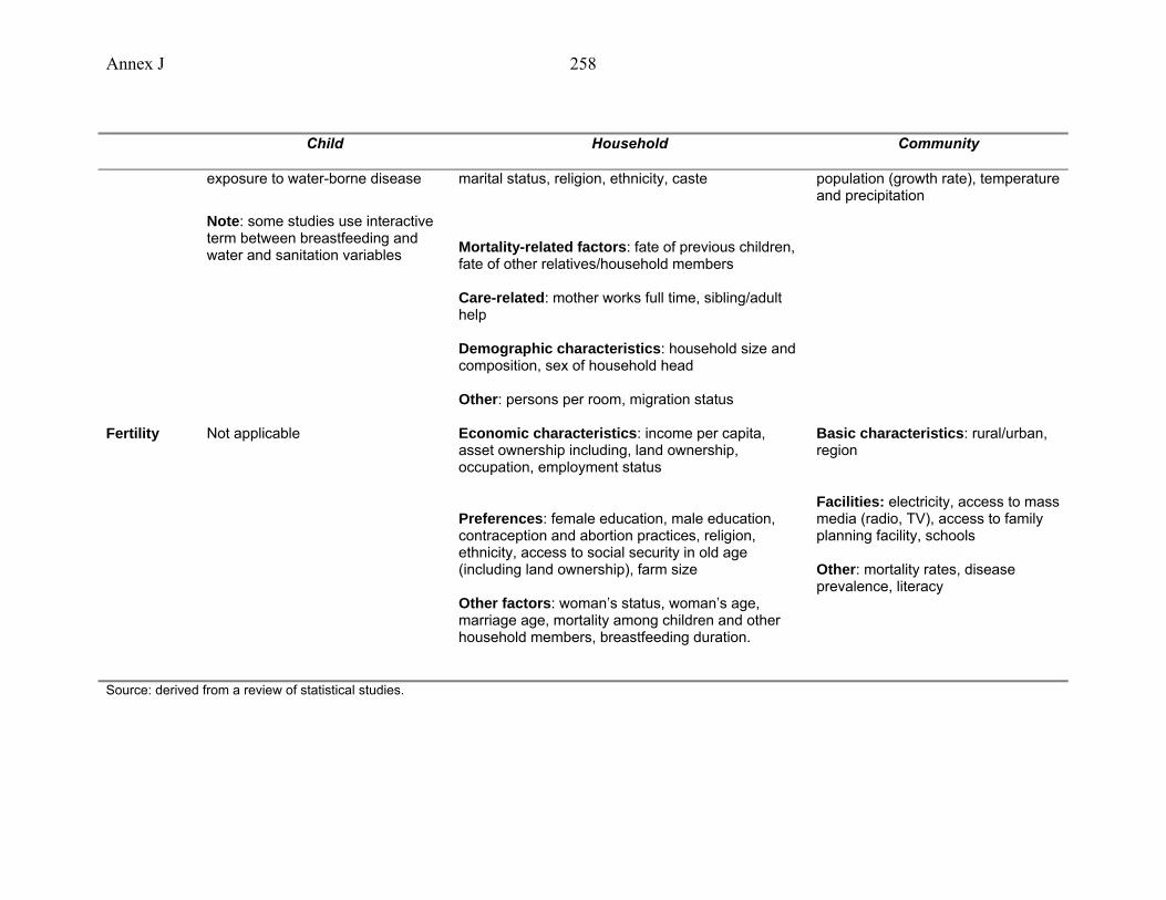
Annex J

258

Child Household Community

exposure to water-borne disease

Note: some studies use interactive term between breastfeeding and water and sanitation variables

marital status, religion, ethnicity, caste

Mortality-related factors: fate of previous children, fate of other relatives/household members Care-related: mother works full time, sibling/adult help Demographic characteristics: household size and composition, sex of household head Other: persons per room, migration status

population (growth rate), temperature and precipitation

Fertility Not applicable Economic characteristics: income per capita, asset ownership including, land ownership, occupation, employment status

Preferences: female education, male education, contraception and abortion practices, religion, ethnicity, access to social security in old age (including land ownership), farm size Other factors: woman’s status, woman’s age, marriage age, mortality among children and other household members, breastfeeding duration.

Basic characteristics: rural/urban, region

Facilities: electricity, access to mass media (radio, TV), access to family planning facility, schools Other: mortality rates, disease prevalence, literacy

Source: derived from a review of statistical studies.

259

References Agarwal, B. (1990) Gender Relations and Food Security: Coping with Seasonality, Drought, and

Famine in South Asia, PEW/Cornell lecture series on food and nutrition policy, Nov 13, CFNPP Publications, Washington DC.

Alauddin, M. and Hossain, M. (2001) Environment and Agriculture in a Developing Economy: Problems and Prospects for Bangladesh, Edwar Elgar, Northampton, MA.

Alauddin, M. and Tisdell, C. A. (1998) The environment and economic development in South Asia: an overview concentrating on Bangladesh, Macmillan Press Ltd, London.

Alderman, H. and Garcia, M. (1994) “Food security and health security: Explaining the levels of nutritional status in Pakistan,” Economic Development and Cultural Change, 42 (3), 485-507.

Alderman, H. and J. R. Behrman (2003), Estimated Economic Benefits of Reducing LBW in Low-Income Countries, Philadelphia, PA: University of Pennsylvania mimeograph (for Human Development Network/Nutrition, World Bank).

Alderman, H. Hentschel, J. and Sabates, R. (2003) “With the help of one’s neighbors: externalities in the production of nutrition in Peru,” Social Science and Medicine, 56 (10), 2019-2031

Ateng, B. (1998) ‘Comparative advantage and crop diversification’ in Faruqee, R. (ed), Bangladesh Agriculture in the 21st Century, The University Press Ltd, Dhaka.

Baffes, J. and Gautam, M. (1996) Is Growth in Bangladesh’s Rice Production Sustainable?, Policy Research Working Paper 1666, The World Bank, Washington D.C.

Bairagi R, M. Mazharul Islam and M.K Barua, 1996, Contraceptive Failure: Levels, Trends and Determinants in Matlab, Bangladesh, Population Studies Center, ICDDR’B, Dhaka (mimeo).

Bairagi, R. (1980) “Is income the only constraint on child nutrition in rural Bangladesh?” Bulletin of the World Health Organization, 58 (5), 767-772.

Bairagi, R. (1986) “Food crisis, nutrition, and female children in rural Bangladesh,” Population and Development Review, 12 (2), 307-315.

Bairagi, R. (1996) ‘Is Son Preference an Obstacle to Fertility Transition in Bangladesh’ in IUSSP Committee on Fertility and Family Planning, Population Council Islamabad, Rockefeller Foundation & UNFPA Pakistan Office, Comparative Perspectives on Fertility Transition in South Asia, IUSSP: Liege

Bairagi, R., Chandra Sutradhar, S. and Alam, N. (1999) “Levels, trends and determinants of child mortality in Matlab, Bangladesh, 1966-94,” Asia-Pacific Population Journal, 14, 2, 51-68.

Bangladesh Bureau of Statistics (2000) Statistical Pocketbook of Bangladesh, BBS, Ministry of Planning Bangladesh.

260

Bangladesh Contraceptive Prevalence Survey (CPS) 1991, 1989, 1983, 1979;

Bangladesh Fertility Survey (BFS) 1989

Bangladesh Retrospective Survey of Fertility and Mortality (BRSFM) 1974.

Barkat, Abul, S.H. Khan, M. Rahman, S. Zaman, A. Podder, S. Halim, N.N. Ratna, M. Majid, A.K.M. Maksud, A. Karim, S. Islam (2002) Economic and Social Impact Evaluation Study of the Rural Electrification Program in Bangladesh Human Development Research Centre and NRECA International Ltd.

Baulch, Bob and John Hoddinott (eds.) (2000) ‘Economic Mobility and Poverty Dynamics in Developing Countries,’ Special Issue, Journal of Development Studies, 36.

Beaton G.H and H. Ghassemi (1982), Supplementary Feeding Programs for Young Children in Developing Countries, American Journal of Clinical Nutrition, 863:916.

Becker, S. and Weng, S. (1998) ‘Seasonal patterns of deaths in Matlab, Bangladesh’, International Journal of Epidemiology, 1999: 27: 814-23.

Begum Sharifa --------------, 2003, Abortion in Rural Bangladesh: Nature, Causes, Problems and Practices, Research Report No. 174, BIDS, Dhaka.

Begum Sharifa, 1976, An Estimation of Birth and Death rate in Bangladesh, 1951-60, IIPS, Bombay India (mimeo)

Begum Sharifa---------------, 1990, Population Birth, Death and Growth Rates in Bangladesh: Census Estimates, The Bangladesh Development Studies, Vol.18, No.2, Dhaka.

Berg A. (1983), Nutrition Review, Population and Human Resources Department, World Bank, Washington DC.

Bhuiya, A. and Chowdhury, M. (1997) “The effect of divorce on child survival in a rural area of Bangladesh,” Population Studies, 51, 57-61.

Bhuiya, A. and Streatfield, K. (1991) “Mothers’ education and survival of female children in a rural area of Bangladesh,” Population Studies, 45, 253-264.

Blanc Ann, 1990, The Relationship between Contraceptive Prevalence and Total Fertility in DHS Countries (Columbia, Maryland: Demographic and Health Surveys Project).

Bloem, M. W.; Moench-Pfanner, R., Panagides, D. (eds) (2003) Health and Nutritional Surveillance for Development, Hellen Keller Worldwide, Singapore.

Bloem, M., Moench-Pfanner, R. and Panagides, D. (eds) (2003) Health and Nutritional Surveillance for Development, Singapore: Helen Keller Worldwide.

Bollen, Kenneth A., Jennifer L. Glanville, Guy Stecklov (1999) ‘Socioeconomic Status and Class in Studies of Fertility and Health in Developing Countries,’ University of North Carolina at Chapel Hill, February 1999.

261

Bollen, Kenneth A., Jennifer L. Glanville, Guy Stecklov (2002) 'Economic Status Proxies in Studies of Fertility in Developing Countries: Does the measure matter?' Population Studies, 56: 81-96.

Bongaart John -------and R.G. Potter, 1983, Fertility Behavior: Biological Analysis of the Proximate Determinants of Fertility, New York, Academic Press.

Bongaart John, 1978, A framework for Analyzing the Proximate Determinants of Fertility, Population and Development Review, Vol.4(1).

Briend, A., Dykewicz, C., Graven, K., Mazumder, R., Wojtyniak, B. and Bennish, M. (1986) “Usefulness of nutritional indices and classifications in predicting death of malnourished children,” British Medical Journal, 293, 373-375.

Brown, K. H.; Black, R.E.; Becker, S. (1982) Seasonal changes in nutritional status and the prevalence of malnutrition in a longitudinal study of young children in rural Bangladesh, in The American Journal of Clinical Nutrition, 36: August.

Buhmann et al., (1988), ‘Equivalence Scales, Well-being, Inequality and Poverty,’ Review of Income and Wealth, 34: 115-142; cited in Wagstaff (2000: 23).

Caldwell, J., Barkat-Khuda, B. Cladwell, I. Pieris and P. Cladwell (1999) “The Bangladesh Fertility Decline: an interpretation” Population and Development Review 25(1) 67-84.

Carvalho, S. and H. White (2004) “Theory-based evaluation: the case of social funds” American Journal of Evaluation 25(2) 141-60.

Chamabagwala, Rubiana, Martin Ranger, Hugh Waddington and Howard White (2004) ‘The determinants of child health and nutrition: a meta-analysis’ OED Working Paper. Washington D.C.: World Bank.

Charmarbagwala, R., Ranger, M., Waddington, H. and White, H. (2004) “The determinants of child health and nutrition: a meta-analysis,” Mimeo, Operations Evaluation Department, Washington, DC: The World Bank.

Chatterjee M. (1991), Towards Better Health for Indian Women: the Dimensions, Determinants and Consequences of Female ‘Illnesses’ and ‘Death’, World Bank, Washington DC.

Chaudhury, Nazmul and Jeffrey Hammer ‘Ghost Doctors: absenteeism in Bangladeshi Health Facilities’, World Bank Working Paper No. 3065, May 2003.

Chen, L., Chowdhury, A. and Huffman, S. (1980) “Anthropometric assessment of energy-protein malnutrition abd subsequent risk of mortality among pre-school aged children,” American Journal of Clinical Nutrition, 33, 1836-1845.

Chen, L., Huq, E. and D’Souza, S. (1981) “Sex bias in the family allocation of food and health care in rural Bangladesh,” Population and Development Review, 7, 55-70.

Chowdhury, M. & Bairagi, R. (1990) ‘Son preference and fertility in Bangladesh’, Population and Development Review, 16:4.

262

Chowdhury, M. A. T. and Zulfikar, H. (2001) An Agricultural Statistical Profile of Bangladesh, 1947-1999, CGPRT Centre, Bogor, Indonesia.

Christiaensen L. and H. Alderman (2004), Child Malnutrition in Ethiopia: Can Maternal Knowledge Augment the Role of Income?, Economic Development and Cultural Change, Vol. 52, No. 2, pp. 287-312.

Cleland John and Kim Streatfield, 1992, The Demographic Transition: Bangladesh, UNICEF, Dhaka, Program Planning Unit.(mimeo).

Cleland John, Philips F.James, Amin Sajeda, Kamal GM, 1994, The Determinants of Reproductive Change in Bangladesh “Success in Challenging Environment”, The World Bank, Washington, DC.

Cleland, John (1994) The Determinants of reproductive change in Bangladesh: success in a challenging environment. Washington D.C.: World Bank.

Cockcroft, Anne, Debbie Milne and Neil Andersson (2003) Bangladesh: HPSP, 1998-2003. Third Service Delivery Survey 2003. Dhaka: CIETcanada.

Croll, E. (2001) Endangered daughters: discrimination and development in Asia, London: Routledge.

Davis K, and Judith Blake, 1956, Social Structure and Fertility: An Analyitical Framework, Economic Development and Cultural Change, Vol.4. No.2.

Del Ninno, C.; Dorosh, P. A.; Smith, L. C. and Roy, D. K. (2001), The 1998 Floods in Bangladesh – Disaster Impacts, Household Coping Strategies, and Response, International Food Policy Research Institute, Washington DC.

Deolalikar, A. (2002) “Poverty and child malnutrition in Bangladesh,” Bangladesh Poverty Assessment Background Paper #7.

EM-DAT (2004) The OFDA/CRED International Disaster Database, www.em-dat.net , Université catholique de Louvain, Brussels.

Fairlie, R. (2003) “An extension of the Blinder-Oaxaca decomposition technique to logit and probit models,” Economic Growth Center Discussion Paper no. 873, New Haven: Yale University.

Faruqee, R. (ed) (1998) Bangladesh Agriculture in the 21st Century, The University Press Ltd, Dhaka.

Faveau V., Koenig M.A., Chakraborty J. and A.I Chowdhury (1988), Causes of maternal mortality in rural Bangladesh, 1976-85, Bulletin of the World Health Organization, 66(5), pp. 643-651.

Faveau, V., Briend, A., Chakraborty, J. and Sarder, A. (1990) “The contribution of severe malnutrition to child mortality in rural Bangladesh: Implications for targeting nutritional interventions,” Food and Nutrition Bulletin, 12, 215-222.

263

Filmer, D. and L. Pritchett (1999) “The impact of public spending on health: does money matter?” Social Science and Medicine 49(10):1309-23.

Filmer, Deon and Lant Pritchett (1998) ‘Estimating Wealth Effects Without Income or Expenditure Data – Or Tears: Educational Enrolment in India,’ World Bank Policy Research Working Paper No, 1994. Development Economics Research Group, World Bank, Washington, DC.

Filmer, Deon and Lant Pritchett (1999) ‘The Effect of Household Wealth on Educational Attainment: Evidence from 35 Countries,’ Population and Development Review, 25 (1): 85-120.

Fine P. (1993) ‘Herd immunity: history, theory, practice’ Epidemiology Review 15:265-302)

Foster, A., J. Greer and E. Thorbecke (1984) ‘A Class of Decomposable Poverty Measures,’ Econometrica, 52: 761-766.

Gage, A., E. Sommerfelt and A. Piani (1996) ‘Household Structure, Socioeconomic Level, and Child Health in Sub-Saharan Africa,’ Demographic and Health Surveys Analytical Reports No. 1.

Gomez, F., Galvin, R., Frenk, S., Cravioto, J., Chavez, R. and Vasquez, J. (1956) “Mortality in second and third degree malnutrition,” Journal of Tropical Pediatrics, 2, 77-83.

Goodburn, Elizabeth A, Mushtaque Chowdhury, Rukhsana Gazi, Tom Marshall and Wendy Graham (2000) “Training traditional birth attendants in clean delivery does not prevent postpartum infection” Health Policy and Planning 15(4): 394-399

Government of Bangladesh (2002) Interim Poverty Reduction Strategy Paper.

Government of the People’s Republic of Bangladesh/IMF (2003) Bangladesh: Interim Poverty Reduction Strategy Paper, IMF, Washington, DC.

Government of the People’s Republic of Bangladesh/International Monetary Fund (2003) A National Strategy for Economic Growth, Poverty Reduction and Social Development, Economic Relations Division, Ministry of Finance, Government of Bangladesh.

Green, W. (1998) “Gender economics courses in liberal arts colleges: further results,” Journal of Economic Education, Fall 1998.

Greene, W.H. (2000) Econometric Analysis, Fourth Edition, New York: Prentice Hall.

Griffiths M., Dickin K. and M. Favin (1996), Promoting the Growth of Children: What Works. Rationale and Guidance for Programs, World Bank, Washington DC.

Grosh, M. & P. Glewwe (2000) Designing Household Survey Questionnaires for Developing Countries: Lessons from 15 Years of the Living Standards Measurement Study, 3 Volumes, The World Bank, Washington, DC.

264

Gwatkin, Davidson R., Shea Rustein, Kierston Johnson, Rohini P. Pande and Adam Wagstaff (2000) Socio-Economic Differences in Health, Nutrition and Population in Bangladesh, HNP/Poverty Thematic Group of the World Bank, May 2000, Washington, DC..

Haddad et al. (2003) , L. Alderman, H. S, Appleton, L. Song and Y. Yohannnes. 2003. Reducing malnutrition: How far can income growth take us? World Bank Economic Review. 17(1)

Haider S.J, D. Hussain, I. Nayer, A. Maleque, Ashaduzzaman, and A.R. Khan (2004), Impact Evaluation of Bangladesh Integrated Nutrition Project, IMED and Read, Dhaka.

Haider, S. et al (2004) IMED BINP Evaluation.

Heckman, J. and B, Singer (1984) “Econometric duration analysis,” Journal of Econometrics, 24 (1-2), 63-132.

Horton, S. (1986) “Child nutrition and family size in the Philippines,” Journal of Development Economics, 23, 161-176.

Hossain Shahadat and Others, 1991, Fertility in Bangladesh: Levels and Trends, in proceedings of the Workshop on Dissemination of Current Statistics, November 3-4, 1991, Dhaka.

Hossain, M.; Lewis, D.; Bose, M. L.; Chowdhury, A. (2003) Rice Research, Technological Progress, and Impacts on the Poor: The Bangladesh Case (Summary Report), EPTD Discussion Paper No. 110, IFPRI, Washington D.C.

Hossain, Z. and A.F.H. Choudhury (1987), Folk Dietary Practices and Ethnophysiology of Pregnant Women in Rural Bangladesh, Michigan State University Working Paper 137.

Houweling, Tanya, Anton Kunst and Johan Mackenbach (2003) ‘Measuring Health Inequality Among Children in Developing Countries: Does the choice of the indicator of economic status matter?’ International Journal for Equity in Health, 2(1): 8-21.

Howlader, A.A. and Bhuiyan, M.U. (1999) “Mothers’ health-seeking behaviour and infant and child mortality in Bangladesh,” Asia-Pacific Population Journal, 14, 1, 59-75.

Huq Md.Nazmul and John Cleland, 1990, Bangladesh Fertility Survey-1989, NIPORT, Dhaka.

Institute of Medicine (1990), Nutrition During Pregnancy, National Academy Press, Washington DC.

International Rice Research Institute (2004):http://www.irri.org/science/ricestat/index.asp

Islam Atahar et.al, 2001, Plateauing of Fertility Level in Bangladesh: Exploring the Reality, Paper 18, CPD-UNFPA Program on Population and Sustainable Development, CPD, Dhaka.

Islam M.A, MM Islam and N Chakraborty, 2001, Plateauing of Fertility Level in Bangladesh: Exploring the Reality, Paper No.18, CPD-UNFPA Program on Population and Sustainable Development, CPD, Dhaka.

265

Jaim, W. M. H. (1984) ‘Changes in Output and Employment due to New Technology: A Study in an irrigated Area of Bangladesh’, in Economic Affairs 29: 35-42.

Kabeer, Naila (2001a) ‘Ideas, Economics and 'the Sociology of Supply: Explanations for Fertility Decline in Bangladesh Journal of Development Studies

Kabir M and Abdullah AL Mamun Chowdhury, 2004, Plateauing Fertility in Bangladesh: Correlates and Proximate Determinants, in Ubaidur Rob et. al. (ed.); Fertility Transition in Bangladesh: Evidence and Implication, UNFPA, Dhaka

Kabir, M. and Amin, R. (1993) “factors influencing child mortality in Bangaldesh and their implications for the national health programme,” Asia-Pacific Population Journal 8, 3, 31-46.

Kakwani, N. (1980) Income inequality and poverty: Methods of estimation and policy Applications, New York: Oxford University Press.

Kakwani, N., Wagstaff, A. and van Doorslaer, E. (1997) “Socioeconomic inequalities in health: measurement, computation and statistical inference,” Journal of Econometrics, 77(1): 87-104.

Kantner A and Elizabeth Frankenberg, 1986, “Levels and Trends in Fertility and Mortality in Bangladesh”, in Bangladesh Contraceptive Prevalence Survey-1985: Secondary Analysis, Mitra and Associates, Dhaka.

Kantner Andrew and Ali Noor, 1992, Population Dynamics in Bangladesh: Current Demographic Estimates and Future Prospects, East-West Center and Office of the Population and Health,USAID, Dhaka (mimeo).

Karim, R; Lamstein, S. A.; Akhtaruzzaman, M.; Rahman, K. M.; Alam, N. (2003) The Bangladesh Integrated Nutrition Project: Endline Evaluation of the Community Based Nutrition Component, The Insititute of Nutrition and Food Sciences University of Dhaka, Bangladesh and The Friedman School of Nutrition Science and Policy, Tufts University, USA.

Khan, M. A. & Khanum, P. A. (2000) Influence of Son Preference on Contraceptive Use in Bangladesh, Asia-Pacific Population Journal, September; 43-54.

Khan, M.M. and Yoder, R.A. (1998) “Expanded Program on Immunization in Bangladesh: Cost, Cost-Effectiveness, and Financing Estimates” Special Initiatives Report No. 6, Partnerships for Health Reform, Bethesda MD.

Kishor, Sunita and Sulabha Parasuraman (1998) ‘Mother’s Employment and Infant and Child Mortality in India,’ National Family Health Survey Subject Reports, Number 8 (April).

Koenig, Michael, Phillips, James, Campbell, Oona and D’Souza, Stan (1990) “Birth intervals and childhood mortality in rural Bangladesh,” Demography, 27, 2, 251-265.

Kramer M.S. (1987), Determinants of low birth weight: methodological assessment and meta-analysis, Bulletin of the World Health Organization, 65(5), 663-737.

266

Kramer M.S., (2001) A New and Improved Population-based Canadian Reference for Birth Weight for Gestational Age, Pediatrics, electronic version, August, 2001.

Lavy, V., Strauss, J., Thomas, D. and de Vreyer, P. (1996) “Quality of health care, survival and health outcomes in Ghana,” Journal of Health Economics, 15, 333-357.

Lee, L.-f., Rosenzweig, M. and Pitt. M. (1997) “The effects of improved nutrition, sanitation, and water quality on child health in high-mortality populations,” Journal of Econometrics, 77, 209-235.

Levinson, M.; Halpern, O.; Mahmud, Z.; Chowdhury, S. A.; Levinson, J. F. (2002) Nutrition-Related Caring Practices and Women’s Time Constraints: A Study in Rural Bangladesh, TUFTS Nutrition, Food Policy and Applied Nutrition Program, Discussion Paper No. 18.

Levitt, MJ. (1999 ). “When the Training of TBAs is Cost Effective: Trained TBAs and Neonatal Essential Care in South Asia,” in Anthony Costello and Dharma Manandhar (eds.) Improving Newborn Infant Health in Developing Countries.. London: Imperial College Press.

Mabud M.A, 1987, Levels and Trends in Fertility and Demographic Prospects in Bangladesh, in

M.A Mabud (ed.) Recent Trend in Fertility and Mortality in Bangladesh, Proceedings of a National Seminar, June 11-13, 1987, PDEU, Planning Commission, Dhaka

Mackenbach J.P., Kunst A.E. (1997) “Measuring the magnitude of socio-economic inequalities in health: an overview of available measures illustrated with two examples from Europe,” Social Science and Medicine, 44: 757-771.

Madise, N.J., Z. Matthews and B. Margetts (1999) ‘Heterogeneity of Child Nutritional Status between Households: A comparison of six sub-Saharan African Countries,’ Population Studies, 53: 331-343.

Mahmud, W. (1998) ‘Comparative advantage and crop diversification’ in Faruqee, R. (ed), Bangladesh Agriculture in the 21st Century, The University Press Ltd, Dhaka.

Mahmud, W.; Rahman, S. H.; Zohir, S. (1994) Agricultural growth through crop diversification in Bangladesh, Working Papers on Food Policy in Bangladesh, No. 7, IFPRI, Washington D.C.

Martorell R. and M. Shekar (1992), Growth-faltering Rates in California, Guatemala, and Tamil Nadu: Implications for Growth-Monitoring Programs, Food and Nutrition Bulletin, Vol. 5, No.3.

Mason J.B, J. Hunt, D. Parker, and U. Johnson (2001), Improving Child Nutrition in Asia, Food and Nutrition Bulletin, Vol. 22, No. 3 (Supplement), United Nations University Press, Tokyo.

Masset, E. and White, H. (2003) “Infant mortality in Andhra Pradesh, analyzing changes over time and between states,” Young Lives Working Paper no. 6.

267

Masset, Edoardo and Howard White (2002) ‘Infant and Child Mortality in Andhra Pradesh: Analysing changes over time and between states,’ Young Lives Working Paper No. 8.

Mian, W. M. A. (ed) (2001) Agricultural Research in Bangladesh in the 20th century, Bangladesh Agricultural Research Council and Bangladesh Academy of Agriculture, Dhaka.

Miller, Jane E. (1989) “Is the relationship between birth intervals and perinatal mortality spurious? Evidence from Hungary and Sweden,” Population Studies, 43, 3, 479-495.

Ministry of Health and Population Control, GOB, 1978, World Fertility Survey: Bangladesh Fertility Survey, 1975; First Report, Dhaka.

Mitra S.N, et.al. 1994, Bangladesh Demographic and Health Survey: 1993-94, NIPORT, Mitra & Assocaites and Macro International Inc.

Mitra, S., Ali, M., Islam, S., Cross, A. and Saha, T. (1994) Bangladesh Demographic and Health Survey, 1993-94, Calverton, Maryland: National Institute of Population Research and Training (NIPORT), Mitra and Associates and Macro International Inc.

Mitra, S., Al-Sabir, A., Cross, A. and Jamil, K. (1997) Bangladesh Demographic and Health Survey, 1996-97, Calverton, Maryland: National Institute of Population Research and Training (NIPORT), Mitra and Associates and Macro International Inc.

Moore, Mick (2003) ‘Politics and the Drivers of Pro-Poor Change in Bangladesh’, report to DFID, Dhaka.

Mosley, W. and Chen, L. (1984) “An analytical framework for the study of child survival in developing countries,” Population and Development Review, Supplement to vol. 10.

Mozumder, A., Barkat-E-Khuda, Kane, T., Levin, A. and Ahmed, S. (2000) “The effect of birth interval on malnutrition in Bangladeshi infants and young children,” Journal of Biosocial Science, 32, 289-300.

Muhiri, P. and Menken, J. (1997) “Adverse effects of next birth, gender, and family composition on child survival in Bangladesh,” Population Studies, 51, 3, 279-294.

Muhuri, P. and Preston, S. (1991) “Effects of family composition on mortality differentials by sex among children in Matlab, Bangladesh,” Population and Development Review, 17, 3, 415-433.

Muhuri, R. (1996) “Estimating seasonality effects on child mortality in Matlab, Bangladesh,” Demography, 33 (1), 98-110.

Nag M. (1994), Beliefs and Practices about Food During Pregnancy, Economic and Political Weekly, Sept 10, 2427-2438.

National Environment Agency, Singapore: http://app.nea.gov.sg/cms/htdocs/article.asp?pid=1099

268

National Institute of Population Research and Training (NIPORT), Mitra and Associates and ORC Macro (2001) Bangladesh Demographic and Health Survey: 1999-2000, Calverton, Maryland: NIPORT, Mitra and Associates and ORC Macro.

National Institute of Population Research and Training (NIPRT) (2002), Bangladesh Maternal Health Services and Maternal Mortality Survey 2001, Measure/DHS+.

NIPORT, Mitra and Assocates and Macro International Inc. 2001, Bangladesh Demographic and Health Survey, 1999-2000, Dhaka.

Operations Evaluation Department (OED) (2004) Impact Evaluation of external support on maternal and child health in Bangladesh, Design Paper, May 2004, Mimeo, Washington, DC: The World Bank.

Palloni, A. and Tienda, M. (1986) “The effects of breastfeeding and pace of childbearing on mortality at early ages,” Demography 23, 1, 31-52.

Pedersen, KM (2002) “TheWorld Health Report 2000: dialogue of the deaf?” Health Economics 11: 93–10.

Pelletier D.L. and E.A. Frongillo (2003), Changes in Child Survival Are Strongly Associated with Changes in Malnutrition in Developing Countries, Journal of Nutrition, No. 133, pp. 107-119.

Pitt, M. and Khandker, S. R. (2002) ‘Credit Programmes for the Poor and Seasonality in Rural Bangladesh’, in The Journal of Development Studies, 39:2.

Podja, J. and L. Kelley (2000), Low Birth-Weight, ACC/SCN (Administrative Committee on Coordination/Sub-Committee on Nutrition), nutrition policy paper No. 18.

Rabbani AKMA Ghulam and Shahadat Hossain, 1984, Levels of Fertility and Mortality from the National Sample Vital Registration System, Paper Presented at the National Seminar on Recent Trends in Fertility ad Mortality in Bangladesh, PDPU, Planning Commission, Dhaka, January 29-31, 1984.

Razzaque, A., Alam, N., Wai, L. and Foster, A. (1990) “Sustained effects of the 1974-5 famine on infant and child mortality in a rural area of Bangladesh,” Population Studies, 44, 145-154.

Rele J.R, ----------, 1987, Fertility Levels and Trends in India, 1951-81, Population and Development Review, Vol.13, No.3.

Rele J.R, 1976, Fertility Analysis Through Extension of Stable Population Concepts, Greenwood Press, Westport, Connecticut, 1976.

Reutlinger S. and M. Selowsky (1976), Malnutrition and Poverty, World Bank Staff Occasional Papers No. 23, Washington DC.

Rogal, B.; Harrisss, B. W. and Bose, S. (eds) (1999) Sonar Bangla? Agricultural Growth and Agrarian Change in West Bengal and Bangladesh, Sage Publications, Thousand Oaks, CA

269

Rosenzweig, M. and Schultz, T.P. (1983) “Estimating a household production function: heterogeneity, the demand for health inputs, and their effects on birth weight,” Journal of Political Economy, 91 (5), 723-746.

Rosenzweig, M. and Schultz. T.P. (1983) “Estimating a household production function: Heterogeneity, the demand for health inputs, and their effects on birth weight,” Journal of Political Economy, 91 (5), 723-746.

Ross. J and E. Frankenberg, 1993, Findings from Two Decades of Family Planning Research, The Population Council.

Rutstein. S. (1984) “Infant and child mortality: levels, trends and demographic differentials,” WFS Comparative Studies 43, Voorburg, The Netherlands: International Statistical Institute.

Sahn, David and David Stifel (2000) 'Poverty Comparisons Over Time and Across Countries in Africa, World Development, 28 (12): 2123-2155.

Sastry, Narayan (1996) ‘Community Characteristics, Individual and Household Attributes, and Child Survival in Brazil,’ Demography, 33 (2): 211-229.

Save the Children (2003), Thin on the Ground. Questioning the Evidence Behind World Bank-funded Community Nutrition Projects in Bangladesh, Ethiopia and Uganda, Save the Children UK, London.

Save the Children (2004) Thin on the Ground. London: Save the Children.

Sen, A. (1998) “Mortality as an indicator of economic success and failure,” Economic Journal, 108, no. 446, 1-25.

Sibley LM and Sipe TA (2004). “What can a meta-analysis tell us about traditional birth attendant training and pregnancy outcomes?” Midwifery 20, 51-50.

Smith, L. and L. Haddad (2000) Explaining Child Malnutrition in Developing Countries: a cross-country analysis. Washington D.C.: IFPRI.

Streatfield, P., Mercer, A., Siddique, A., Ziauddin, A., Ashraf, A. (2003) Status of Performance Indicators, 2002, Health & Population Sector Programme, 1998-2003, A report for the Health Programme Support Office for the Annual Programme Review 2002, Dhaka: International Centre for Diarrhoeal Disease Research, Bangladesh

Thomas, D., Strauss, J. and Henriques, M-H. (1991) “How does mother’s education affect child height?” Journal of Human Resources, 26 (2), 183-211.

Thomas, D., Strauss, J. and Henriques, M-H. (1991) “How does mother’s education affect child height?” Journal of Human Resources, 26 (2), 183-211.

UNICEF (1990) Strategy for improved nutrition of children and women in developing countries, New York: UNICEF.

270

UNICEF (2002) State of the World’s Children 2003, New York: UNICEF.

Vemury, M. (1981), Rural Food Habits in Six Developing Countries: a CARE Studyoif Environmental, Social and Cultural Influence on Food Consumption Patterns, New York: CARE.

Wagstaff, A. (2000) “Unpacking the causes of inequalities in child survival: The case of Cebu, The Philippines,” Mimeo, Washington, DC: The World Bank.

Wagstaff, Adam (2000) ‘Socioeconomic Inequalities in Child Mortality: Comparisons across nine developing coutries,’ Bulletin of the World Health Organisation, 78(1).

Wagstaff, Adam and Naoko Watanabe (2002) What Difference does the Choice of SES Make in Health Inequality Measurement? Development Research Group, The World Bank, Washington, DC.

Waterlow J.C. (1992), Protein-energy malnutrition, Edward Arnold, London.

Weiss, C. (1998) Evaluation Upperr Saddle River, NJ: Prentice Hall.

White, Howard and Edoardo Masset (2003) ‘The Importance of Household Size and Composition in Constructing Poverty Profiles: An illustration from Vietnam,’ Development and Change, 34(1): 105-126.

WHO Expert Committee (1995), Physical Status: The Use and Interpretation of Anthropometry, WHO Technical Report Series No. 854, Geneva.

World Bank (1995), Staff Appraisal Report. Bangladesh Integrated Nutrition Project, Population and Human Resources Division, Washington D.C.

World Bank (2002) ‘Poverty in Bangladesh: building on progress’. Washington D.C.: World Bank.

Young Lives: An international study of childhood poverty (2002) Justification of the Content of the Household Questionnaires, Section 9: Socio-economic status.

Zenger, E. (1993) “Siblings’ neonatal mortality risks and birth spacing in Bangladesh,” Demography, 30, 3, 477-488.

Documents

Maintaining Momentum Towards the MDGs: An Impact ... · An Impact Evaluation of Interventions to Improve ... Document of the World Bank ... to Meera Shekar of the World Bank’s nutrition