Embed Size (px)
Citation preview
MAKING WAVES
THE EFFECTS OF BOAT-WASH ON MACROBENTHIC ASSEMBLAGES OF ESTUARIES
Melanie J. Bishop
A thesis submitted in fulfillment of the requirements for the degree of Doctor of Philosophy in the University of Sydney
April 2003
The work contained within this thesis, except where otherwise acknowledged, is the result of my own investigations
Signed: Date:
ABSTRACT
Numerous studies have examined ecological impacts of boating resulting from scarring
by propellers, the discharge of pollutants and sewage, noise, anchoring and the infrastructure
associated with boating (e.g. marinas and wharves). Only recently have studies considered the
impact of wash. This is the loose water produced by a vessel as it travels through the water.
Most studies have focussed on wash produced by fast-ferry services. It is, however, known
that wind-generated waves, which are typically smaller and of lesser energy than many boat-
generated waves, are important in determining the distribution and abundance of organisms.
Thus, wash from smaller vessels may also have an impact on estuarine organisms.
This thesis considered: (i) any impact of wash from RiverCat ferries - 35 m, low-wash
vessels that operate on the Parramatta River, Sydney, Australia – on intertidal assemblages
and (ii) the effect of wash on epifauna associated with seagrass blades.
The collapse of seawalls and the erosion of river-banks was observed following the
introduction of RiverCat ferries to the Parramatta River, Sydney, Australia. Several strategies
of management – establishing no-wash zones, where ferries must slow to minimize wash and
planting mangroves, which may dissipate wave-energy – have consequently been
implemented. These were used in mensurative experiments, examining the effects of wash on
infauna. If the establishment of no-wash zones and planting of mangroves are both effective in
minimizing any ecological impact of wash, there should be a greater difference between
assemblages in wash zones (where speed is unrestricted) from those in no-wash zones when
mudflats are sampled than when sampling is done amongst pneumatophores of mangroves.
Along the upper Parramatta River, assemblages of infauna differed between the zones,
regardless of whether sampling was done on mudflats or amongst pneumatophores. The
difference was no greater for organisms in mudflats. Along the lower Parramatta River, where
there is generally less compliance with wash restrictions, no difference was seen. Thus, while
planting mangroves does not appear to be effective in minimizing the ecological impacts of
wash on macro-invertebrates, the establishment of no-wash zones may be.
During the 2000 Sydney Olympic Games, ferry services were suspended for 5 weeks
along the western section of the Parramatta River. This managerial decision provided the
manipulation for an experiment to determine whether patterns between the wash and no-wash
zones of the upper Parramatta River were due to differences in the intensity of wash. If
Abstract
patterns are due to wash, it was hypothesized that, following the removal of the disturbing
force: (i) the assemblages of the wash and the no-wash zones would become more similar and
(ii) abundances of taxa in the wash zone would increase to match abundances in the no-wash
zone. Results supported hypothesis (i) but not hypothesis (ii).
The impact of wash on infauna may be a result of increased rates of mortality of adults
and/or decreased rates of colonization. Any effect of wash may be direct or indirect. Two
experiments were done to determine whether patterns between wash and no-wash zones were
due to a direct or an indirect effect of wash on colonization and/or mortality. The first, which
involved the deployment of units of defaunated sediment, evaluated models attributing the
impact to decreased rates of colonization in the wash zone. If wash directly affects
colonization, differences should be seen between the assemblages accumulating in
homogeneous sediment placed in the wash zone and those in the no-wash zone. If it indirectly
affects colonization via changes to characteristics of the sediment, which, in turn, determine
patterns of colonization, no difference will, however, be seen in the assemblages accumulating
in homogeneous units. A difference will, instead, be seen between the wash zone and the no-
wash zone in the colonization of site-specific sediments. Colonization of sediment was less
spatially variable in the homogeneous than in the site-specific sediment. This indicates that
characteristics of the sediment are important in structuring assemblages. A difference in the
colonization of the wash and no-wash zone was, however, not evident in either of the
treatments.
The second experiment, in which cores of sediment were transplanted within and
between the zones with their associated assemblages, considered direct and indirect effects of
wash on assemblages, resulting from the net effect of mortality of adults and of colonization.
This experiment did not support a direct effect of wash on assemblages but, instead, indicated
that characteristics of the sediment are of primary importance in structuring assemblages.
Abundances of Capitellidae, Nereididae and Amphipoda did, however, increase when
sediment was transplanted from the wash to the no-wash zone and decrease when the
reciprocal transplant was done. This indicates that, while assemblages do not appear to be
directly affected by wash, the abundances of individual taxa are affected.
The second section of this thesis examined the effect of wash on epifauna associated
with seagrass blades through a series of experiments in North Carolina, USA and the Greater
Abstract
Sydney Metropolitan Region. In North Carolina, assemblages of epifauna differed between
places exposed to wash from vessels traveling along the Atlantic Intracoastal Waterway and
places that were sheltered from this disturbance. Abundances of gastropods and amphipods
were smaller in the exposed places.
A possible model for this pattern is that these animals are dislodged from seagrass by the
flapping of the blades as waves propagate through the bed. In the case of mobile organisms,
this model will only explain decreased abundances if the frequency of the disturbance is
greater than the time taken to recolonize the blades, or if organisms are more susceptible to
predation while displaced. If epifauna are indeed displaced by waves, the effect of wash
should be immediate.
It was hypothesized that if a boat were driven past patches of seagrass that are not
usually subject to wash, abundances of small crustaceans and gastropods would decrease
immediately after exposure to wash. This hypothesis was tested at two locations - Narrabeen
and the Georges River. At Narrabeen, results supported the hypothesis. At the Georges River,
in contrast, no change was seen from before to after the disturbance. This may be because this
second location was exposed to strong currents, which may be much more important in
structuring assemblages than wash.
On their own, neither the large-scale mensurative experiments nor the small-scale
manipulative experiments described above, provided much information on the role of wash in
structuring assemblages. Together, however, they showed that, under certain conditions, wash
can reduce the abundance of epifaunal taxa and, where this effect occurs, it is immediate.
Thus, although it is often difficult or even impossible to manipulate large-scale disturbances
directly, observations of these disturbances may be coupled with smaller-scale controlled
manipulative experiments to identify processes that are important in determining the
distribution and abundance of organisms. This study has demonstrated that the large scale of a
disturbance is not a barrier to the experimental test of processes, but rather a unique ecological
opportunity to be exploited.
ACKNOWLEDGEMENTS
First and foremost, I would like to thank Gee Chapman and Tony Underwood for the
considerable contribution they have made to my professional development and the many
opportunities with which they have provided me during my time at the Centre. Without them this
thesis would not be here. In fact, I am fairly certain I would be a plant cell physiologist. Through
their immense enthusiasm they managed to convince me that Marine Ecology was not just a subject
that gave me a good timetable in third year but also an interesting and challenging science. I am
particularly grateful to Gee Chapman, my primary supervisor, for controlling her excitement when
handed the umpteenth piece of paper to read and for managing to keep track of almost all of them!
I would also like to extend a special thank-you to Pete Peterson for allowing me to spend
several months in his lab in North Carolina and providing me with invaluable advice and
encouragement on that phase of my project. What with September 11, the pipe bomb at the boat
ramp and the broken axel on the trailer…I am surprised he has invited me back. Thanks too to the
other members of his lab for their Southern hospitality and to Hal Summerson and David Gaskill for
their help in the field.
To members of the Centre, past and present – I am not even going to try to list everyone who
has provided assistance or made may life in some way more pleasant – thank-you all! I would,
however, like to single out the remaining members of ‘the cohort’ who, after the last four years, are
almost like family to me and who I am going to particularly miss. There’s Katie, with whom I have
shared an office (and the ups and downs of work and social lives) and whose mountain of crap
deflected attention from my not insignificant mess. Brianna, my gym buddy, who is probably the
main reason why, at the end of writing this thesis, I still fit into my jeans. David - always eager to
help a damsel in distress and share a beer…or six. And finally Craig – I’m glad there’s someone else
out there who appreciates real football…no, not league – AFL!!!
My ‘non-Marine’ friends have made sure I have always had a life outside of uni and to them I
owe my sanity. Special thanks to Alex, who has come into my life at the wrong end of my PhD, for
always being there, tolerating my moodiness and not calling me a nerd too many times when I have
gone to uni on a Saturday.
Last, but certainly not least, thanks to my family for all their love and support, for always
encouraging me to follow my dreams and for not booting me out of the family home. It’s amazing
how far an APA can go when you don’t have to pay rent!
TABLE OF CONTENTS Chapter 1 GENERAL INTRODUCTION 1 1.1 The estuarine environment 1 1.2 Disturbances 3 1.3 Boating as a disturbance 4 1.4 Waves as a disturbance to organisms on rocky shores 6 1.5 Waves as a disturbance to organisms in soft-sediments 7 1.6 Previous studies investigating the ecological impacts of boat-wash 8 1.7 Approach used in this thesis 10 SECTION I. RIVERCAT FERRIES: LOW WASH OR BIG SWASH? 13 Chapter 2 RIVERCAT FERRIES ON THE PARRAMATTA RIVER: BACKGROUND AND GENERAL METHODS 14 2.1 The Parramatta River 14 2.2 History of boating on the Parramatta River 16 2.3 RiverCat ferries 18 2.4 Present strategies of management 19 2.5 General Methods 20 2.5.1 Sampling of hard substrata (seawalls) 20 2.5.2 Soft sediment 20 2.5.3 Taxanomic resolution 21 2.6 Analyses 22 2.6.1 Multivariate analyses 22 2.6.2 Univariate analyses 24 Chapter 3 PATTERNS IN THE DISTRIBUTION AND ABUNDANCE OF INTERTIDAL ORGANISMS ON SEAWALLS SHELTERED FROM AND EXPOSED TO THE WASH OF RIVERCAT FERRIES 25 3.1 Introduction 25 3.2 Materials and Methods 27 3.3 Results 30
3.3.1 Initial sampling of assemblages on seawalls close to or further from the RiverCat ferry route 30 3.3.2 Abundances of organisms on seawalls close to or further from the RiverCat ferry route and orientated perpendicular and parallel to the direction of propagation of wash 41 3.3.3 The vertical distribution of sessile organisms on seawalls exposed to and more sheltered from ferry wash 41
3.4 Discussion 46
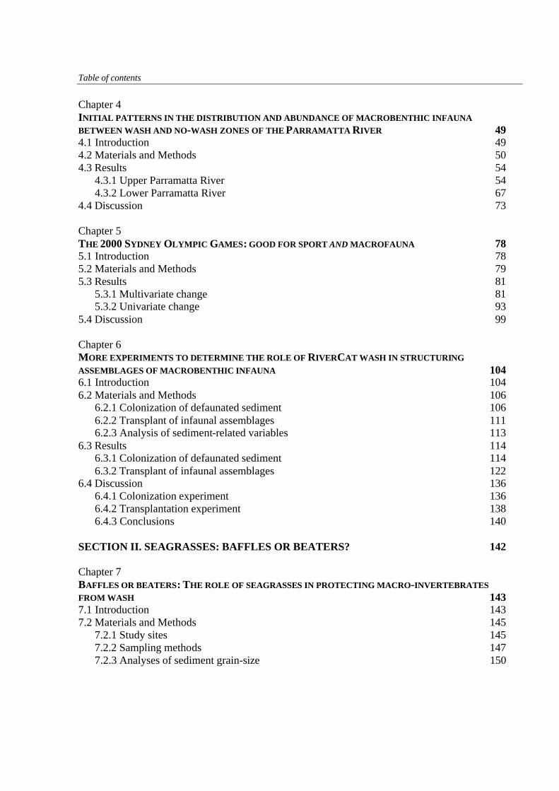
Table of contents
Chapter 4 INITIAL PATTERNS IN THE DISTRIBUTION AND ABUNDANCE OF MACROBENTHIC INFAUNA BETWEEN WASH AND NO-WASH ZONES OF THE PARRAMATTA RIVER 49 4.1 Introduction 49 4.2 Materials and Methods 50 4.3 Results 54 4.3.1 Upper Parramatta River 54 4.3.2 Lower Parramatta River 67 4.4 Discussion 73 Chapter 5 THE 2000 SYDNEY OLYMPIC GAMES: GOOD FOR SPORT AND MACROFAUNA 78 5.1 Introduction 78 5.2 Materials and Methods 79 5.3 Results 81 5.3.1 Multivariate change 81 5.3.2 Univariate change 93 5.4 Discussion 99 Chapter 6 MORE EXPERIMENTS TO DETERMINE THE ROLE OF RIVERCAT WASH IN STRUCTURING ASSEMBLAGES OF MACROBENTHIC INFAUNA 104 6.1 Introduction 104 6.2 Materials and Methods 106 6.2.1 Colonization of defaunated sediment 106 6.2.2 Transplant of infaunal assemblages 111 6.2.3 Analysis of sediment-related variables 113 6.3 Results 114 6.3.1 Colonization of defaunated sediment 114 6.3.2 Transplant of infaunal assemblages 122 6.4 Discussion 136 6.4.1 Colonization experiment 136 6.4.2 Transplantation experiment 138 6.4.3 Conclusions 140 SECTION II. SEAGRASSES: BAFFLES OR BEATERS? 142 Chapter 7 BAFFLES OR BEATERS: THE ROLE OF SEAGRASSES IN PROTECTING MACRO-INVERTEBRATES FROM WASH 143 7.1 Introduction 143 7.2 Materials and Methods 145 7.2.1 Study sites 145 7.2.2 Sampling methods 147 7.2.3 Analyses of sediment grain-size 150
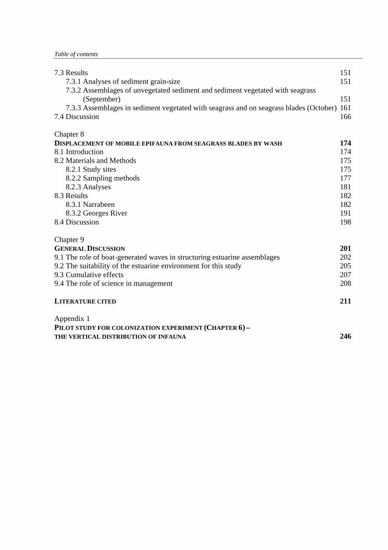
Table of contents
7.3 Results 151 7.3.1 Analyses of sediment grain-size 151
7.3.2 Assemblages of unvegetated sediment and sediment vegetated with seagrass (September) 151 7.3.3 Assemblages in sediment vegetated with seagrass and on seagrass blades (October) 161
7.4 Discussion 166 Chapter 8 DISPLACEMENT OF MOBILE EPIFAUNA FROM SEAGRASS BLADES BY WASH 174 8.1 Introduction 174 8.2 Materials and Methods 175 8.2.1 Study sites 175 8.2.2 Sampling methods 177 8.2.3 Analyses 181 8.3 Results 182 8.3.1 Narrabeen 182 8.3.2 Georges River 191 8.4 Discussion 198 Chapter 9 GENERAL DISCUSSION 201 9.1 The role of boat-generated waves in structuring estuarine assemblages 202 9.2 The suitability of the estuarine environment for this study 205 9.3 Cumulative effects 207 9.4 The role of science in management 208 LITERATURE CITED 211 Appendix 1 PILOT STUDY FOR COLONIZATION EXPERIMENT (CHAPTER 6) – THE VERTICAL DISTRIBUTION OF INFAUNA 246
CHAPTER 1
GENERAL INTRODUCTION
1.1 The estuarine environment
Estuaries are zones of transition between rivers and the sea. They share characteristics of
both, but are identical to neither. The most universally cited definition of an estuary is “a semi-
enclosed coastal body of water which has a free connection with the open sea and within which
sea water is measurably diluted with fresh water derived from land drainage” (Cameron and
Pritchard, 1963). This, however, omits a number of habitats that may be considered estuarine.
Hopkinson and Hoffman (1984) argued that estuarine influences can extend beyond enclosed
waterways to near-shore coastal waters, where seawater is diluted by drainage from land.
According to Hopkinson and Hoffman’s interpretation, the brackish waters of the Amazon and
Mississipi Rivers, which are seaward of their respective river-mouths, are estuarine. In addition,
the Cameron and Pritchard definition does not include coastal lakes and lagoons that are only
intermittently open to the ocean. The salinity of these bodies of water can range from fresh,
during times of heavy rainfall, to hypersaline at times of little rainfall, when evaporation exceeds
the supply of freshwater. Hutchings and Collett (1977) included intermittently open coastal lakes
and lagoons by defining estuaries as the tidal portions of river mouths, bays and coastal lagoons,
irrespective of whether they are dominated by hypersaline, marine or freshwater conditions.
For the purposes of this thesis, “estuary” will be used to describe bodies of water where: (i)
discharge and water-levels are influenced by tidal processes transmitted through a permanent or
intermittent connection with the ocean and (ii) salinity is variable due to mixing of seawater with
freshwater run-off from the land. This definition includes tidal sections of rivers, lagoons and
sounds.
Regardless of the way in which they are defined, estuaries are generally perceived as areas
of great environmental variability. Many are characterized by longitudinal gradients in physico-
chemical variables such as salinity, temperature and the concentration of suspended particulate
matter (Pritchard, 1967). Salinity may range from near 0 to over 35 ppt and sediments may range
from colloids to sands and detritus. Environmental gradients are displaced by the unidirectional
currents of streams and/or oscillating tidal currents (Bassindale, 1943), resulting in large
fluctuations in variables at points within the estuary.
These fluctuations are believed to select against taxa that cannot live and reproduce over a
wide range of environmental conditions (e.g. Sanders, 1969; McLusky, 1981), resulting in a
smaller diversity of species within estuarine habitats than in marine and limnic environments
Chapter 1. General Introduction
2
(Moverley and Hirst, 1999). Sessile organisms are particularly susceptible to large fluctuations at
individual points in an estuary (Kinne, 1971). In many estuaries, the number of species decreases
from the sea towards brackish parts, before increasing again in the direction of the river
(Remane, 1934; Alexander et al., 1935).
In contrast to taxonomic diversity at the scale of individual habitats, functional diversity at
the scale of the estuary is great (Moverley and Hirst, 1999). This is primarily due to the large
range of habitats that estuaries support, which include muddy and sandy beaches, marshes,
mangroves, seagrass meadows, rocky reefs and artificial structures, such as seawalls, pontoons
and pilings (see Ponder et al., 2002). The large diversity at the scale of an estuary may also be
attributed to the diversity of sources from which estuarine fauna are derived – estuaries contain
species from limnic and marine environments, in addition to a unique component (e.g. Day,
1951).
Salt marshes and other wetlands in estuaries frequently export disproportionately large
biomasses of fish and invertebrates, relative to their small area (Boesch and Turner, 1984). These
habitats are often referred to as nursery grounds (e.g. Robertson and Duke, 1987; Laegdsgaard
and Johnson, 1995). The importance of such habitats on the survival, growth and subsequent
entry of juveniles into the adult population scales is, however, unclear. Many of the studies of
fish in mangroves have used inconsistent sampling methods or inadequate sampling designs
(Connolly, 1999, but see Nagelkerken et al., 2000a, 2000b). Properly designed studies, with
appropriate replication and where mangroves and other habitats are sampled at multiple spatial
scales suggest that, at least in urban areas, mangroves may not be particularly important for fish
(Clynick and Chapman, 2002). While unvegetated habitats may appear unproductive, their
assemblages of infauna and epifauna can provide a significant food source for many species of
fish (NSW Fisheries, 1998).
The productivity of estuaries, their location between the oceans and land-masses and their
relatively protected waters, make them valuable resources. They support commercial and
recreational fisheries (e.g. prawns, Broadhurst et al., 1996), are often natural harbours (e.g.
Sydney Harbour, Australia, on the Port Jackson estuary; Poole Harbour, U.K., fed by the Frome
and Piddle Rivers) and/or routes for transportation (e.g. the Atlantic Intracoastal Waterway along
the southeastern coast of the USA). They are also of great social value, being the preferred sites
for human settlement. In New South Wales, Australia, 75% of the population live in towns and
cities near estuaries (NSW DLWC, 2000a). Estuaries are often the cultural centres of coastal
communities, serving as the focal point for local commerce, tourism and recreation. Boating,
Chapter 1. General Introduction
3
fishing, swimming, surfing, and bird-watching are amongst the numerous recreational activities
people enjoy in estuaries.
The high value that society has placed on estuaries for living, working and recreation has,
however, made them one of the most heavily populated and used areas. This great level of
development means that estuaries are subject to a large range of anthropogenic disturbances.
1.2 Disturbances
A disturbance is a process external to a population that causes environmental change
(Underwood, 1989). Disturbances may, or may not, cause changes to the population(s) of
interest. In the case that the disturbance does elicit a response (impact), the cause and effect are
collectively termed a perturbation (Bender et al., 1984).
Glasby and Underwood (1996) identified four types of perturbation according to the time-
scale of the constituent disturbance and response. A perturbation is classified as a ‘discrete pulse’
when both the disturbance and the response are of short duration. When the disturbance is of
short duration, but the effect is sustained, the perturbation is a ‘protracted pulse’. Press
disturbances are of longer duration and, like pulse disturbances, may give rise to responses of a
short (discrete) or long (protracted) temporal scale. These perturbations are termed ‘discrete
presses’ and ‘protracted presses’, respectively.
Disturbance is undisputedly an important factor in determining the structure of aquatic and
terrestrial assemblages (e.g. Cooper, 1926; Watt, 1947; Dayton, 1971; Connell, 1978; Sousa,
1984; Pickett and White, 1985; McGuinness, 1987) and is a major source of temporal and spatial
heterogeneity (reviewed by Sousa, 1984). The severity of a disturbance is determined by its
intensity (physical force of the event per unit area per unit time), frequency (mean number of
disturbing events in a set period of time), area and the nature of its periodicity (cyclic or
stochastic) (Sousa, 1984; Huston, 1994; Townsend et al., 1997). It is, however, unclear how
these variables interact with one another to determine the impact of the disturbance (Death and
Winterbourn, 1995). Most studies have considered the effect of these variables on the severity of
the disturbance independently of one another (e.g. Thrush et al., 1996; Phillips et al., 1997; but
see McCabe and Gotelli, 2000).
In any case, it appears that the relationship between these variables and the severity of the
disturbance is not always linear (Pearson, 1981). For example, gradients of contaminants (i.e.
intensity of disturbance) are often poorly matched with gradients of ecology (Keough and Black,
1996, Raimondi and Reed, 1996). Substrata in the immediate vicinity of industrial-waste and
sewage outfalls are sometimes devoid of benthic macrofauna, with abundances peaking a short
Chapter 1. General Introduction
4
distance from the point of discharge, before decreasing to ‘background’ levels with distance (e.g.
Bellan and Bellan-Santini, 1972; Anger, 1975; Rosenberg, 1976; Bishop et al., 2002). Non-linear
relationships between the frequency of disturbance and diversity of organisms have also been
reported (e.g. AuClair and Goff, 1971; Lubcheco and Menge, 1978; Collins et al., 1995; Hiura,
1995). These studies found greatest diversity of organisms at intermediate frequencies of
disturbance and small diversities at large and small frequencies, supporting the Intermediate
Disturbance Hypothesis, proposed, historically, by Tansley and Adamson (1925) and, in a more
recent context, by Connell (1978).
Characteristics of the environment, the initial structure of the affected assemblage and the
biology of its constituent organisms may also determine the severity of a disturbance. For
example, organisms living in cracks, crevices and rockpools should be less susceptible to the
effects of waves than organisms on exposed substrata (Denny, 1985). The stage in an organism’s
life-cycle at which it is disturbed and the distance over which it can disperse will influence its
susceptibility (see Underwood, 1989).
1.3 Boating as a disturbance
Boating, like most human activities, is a contributing cause to many disturbances in natural
environments. The ecological impacts of boating are of increasing concern given that: (i)
participation rates for recreational boating are on the rise (ii) vessels are becoming larger and
engines more powerful and (iii) development of the coastal zone means that there is better access
to more waterways (Total Environment Centre, 1996).
Boats constitute a potentially significant source of a number of contaminants. These
include organic and inorganic chemicals (e.g. trace elements, tributyltin, polychlorinated
biphenyls, chromated copper arsenate, petroleum hydrocarbons, polynuclear aromatic
hydrocarbons), coliform bacteria and pathogens (e.g. McMahon, 1989; Lenihan et al., 1990;
Weis and Weis, 1992; McGee et al., 1995), which have been found in elevated concentrations
adjacent to marinas and in areas of boating-related activities (e.g. washing down, sanding and
painting, draining bilge water, refuelling; Young et al., 1979; Faust, 1982; Marcus and Stokes,
1985; Valkirs et al., 1986; Langston et al., 1987; McMahon, 1989; Clarisse and Alzieu, 1993;
McGee et al., 1995).
Many studies have examined the effects of contaminants on the biology and ecology of
benthic organisms. Unfortunately, most have provided only circumstantial evidence of impacts.
For example, Waldock et al. (1999) acknowledge that their study on the River Crouch provides
only circumstantial evidence for an effect of tributyltin on assemblages of infauna. Between
Chapter 1. General Introduction
5
1987 and 1992, they found an increase in the diversity of infauna, coincident with a decrease in
the concentration of TBT in the sediment.
Until recently, TBT was added to paint to kill fouling organisms. Despite the paucity of
properly controlled studies examining the impact of TBT on natural assemblages in estuaries, a
large number of studies have reported the same deleterious effects, leaving little doubt as to its
toxicity. TBT has been implicated in causing deformities in oysters (Alzieu et al., 1980; Alzieu
et al., 1981; Waldock and Thain, 1983; Thain and Waldock, 1986) and decimating populations
of dogwhelks (Nucella lapillus) (Bryan et al., 1986; Davies and Bailey, 1991; Evans et al.,
1991), clams (Scrobicularia plana) and whelks (Buccinum unduatum) (Ruiz et al., 1996; ten
Hallers-Tjabbes et al., 1994).
Deleterious effects of polynuclear aromatic hydrocarbons (PAHs), found in petroleum
products, on aquatic organisms have also been documented. PAHs are toxic to many benthic
invertebrates (Sammut and Nickless, 1978; Lee et al., 1981; Widdows et al., 1995; Lee and
Page, 1997) and, in places where the concentrations of PAHs are great, abundances and types of
these organisms are reduced (Olsgard and Gray, 1995). At moderate concentrations, the
environment is made suitable for opportunistic species, which take advantage of the increases in
microflora in response to concentrations of PAHs (Sanders et al., 1980; Bunch, 1987; Steichen et
al., 1996; Lee and Page, 1997).
There is also evidence for a direct physical impact of boating on flora and fauna. Anchors
can cause damage to corals (Davis, 1977; Tilmant and Schmahl, 1981). Macrofauna in sediments
may be displaced by propeller-scarring. Losses of seagrasses have resulted from scouring by
boat-moorings, anchors and propellers (Zieman, 1976; Walker et al., 1989; Hastings et al., 1995;
Creed and Amado Filho, 1999). Although losses are generally small, the scoured area results in
an increase in the length of “edge” which is vulnerable to erosion during storms (Walker et al.,
1989). Regrowth of seagrass is often slow, with recovery rates of Thalassia testudinum in the
Florida Keys requiring an average of 3.5 to 4.1 years (Dawes et al., 1997). Propellers may also
decrease cover of seagrass indirectly through the resuspension of sediment (Gucinski, 1981),
although this is yet to be determined experimentally.
In addition to these disturbances associated with the boats themselves, disturbances related
to facilities associated with boating appear to be important in structuring assemblages of benthic
organisms. Probably the most studied of these is dredging of boating channels, which has been
found to decrease the diversity of assemblages of macrobenthic invertebrates and the abundances
of taxa (Gilmore and Trent, 1974; Kaplan et al., 1974; Daiber et al., 1975; Pfitzenmyer, 1975,
1978; Allen and Hardy, 1980; Van Dolah et al., 1984).
Chapter 1. General Introduction
6
Marinas have also received much attention. The large numbers of artificial substrata
associated with these developments (e.g. pilings and floating pontoons) increase the area of
vertical surface available to fouling organisms, shade hard and soft substrata and obstruct flow of
water (e.g. McGee et al., 1995; Turner et al., 1997). Recent work in Sydney Harbour suggests
that assemblages of sessile invertebrates colonizing these structures are quite different from
those on nearby rocky reefs (Connell and Glasby, 1999; Glasby and Connell, 2001). In addition,
the rooftops and paved surfaces (roads, parking-lots, pavements) associated with marinas and
other boating facilities may increase the stormwater runoff entering estuarine waters. In
developed areas, this run-off can contain contaminants that are toxic or carcinogenic to aquatic
organisms and may affect nutrients, oxygen demand, fecal coliform bacteria, sediment and heat
(US EPA, 1983).
Unfortunately, most of this research has been published only in the grey literature (but see
Connell and Glasby, 1999; Glasby and Connell, 2001) and is relatively inaccessible. Not having
been subject to the scrutiny of a formal process of peer-review, it is also of dubious quality.
Much of this research has used experimental designs that lack sufficient temporal and spatial
replication to be of use in the assessment of ecological impacts (e.g. Pfitzenmyer, 1975, 1978).
Fortunately, with the growing realization that applied research is just as important as pure
research, the number of studies on the ecological impacts of boating in scientific journals appears
to be increasing and the quality of these is improving.
Perhaps the most urgently required research in the area of disturbances due to boating,
then, is on the ecological impact of wash. Wash is the loose water left behind a vessel as it
moves through the water. Despite numerous studies documenting the erosion of shorelines and
the resuspension of sediment by wash (e.g. Anderson, 1976; Hilton and Phillips, 1982; Nanson et
al., 1994; Schoellhamer, 1996), it remains largely unknown whether it has any ecological
impact. Boat wash may be expected to be important in determining the ecology of estuaries
given that: (i) wash from a vessel is similar to wind-driven waves (Stumbo et al., 1999) and (ii)
the well-established role of naturally produced waves in structuring assemblages of soft and hard
substrata.
1.4 Waves as a disturbance to organisms on rocky shores
Oceanic waves are widely documented to be a major force determining the biology and
ecology of rocky shores. Water-motion, associated with the propagation and breaking of waves,
can purportedly affect all stages of the life-history of a marine organism, for example, the
fertilization of gametes (Pennington, 1985; Denny and Shibata, 1989; Levitan, 1991), settlement
Chapter 1. General Introduction
7
of larvae onto hard substrata (Eckman et al., 1990; Bertness et al., 1992), growth (Palumbi,
1984; Koehl and Alberte, 1988) and mortality (Denny et al., 1985; Witman and Suchanek, 1984;
Carrington, 1990). Exposure may also be important in determining the morphology of organisms
(e.g. Trussell et al., 1993; Hobday, 1995; Blanchette, 1997; Ruuskanen, et al., 1999), the
composition of assemblages (Kautsky and Kautsky, 1989; Phillips et al., 1997), patterns of
horizontal and vertical distribution (Seapy and Littler, 1978; Underwood, 1981; McQuaid and
Branch, 1985; Underwood and Jernakoff, 1984; Graham, 1997) and biomass (McQuaid and
Branch, 1985; Ricciardi and Bourget, 1999).
The effects of wave-action on intertidal organisms can be a result of wetting by wash and
spray, or a result of mechanical action of waves (see Southward, 1958; Jones and
Demetropolous, 1968). Two main hydrodynamic forces act on organisms as a result of waves –
drag, which acts in the direction of flow and lift, which is perpendicular to it. These are
approximately proportional to the square of water-velocity (see Denny, 1998 for a more detailed
discussion of drag and lift).
Most of the studies documenting waves to be important in structuring benthic assemblages
have tested their hypotheses by comparing the biota of sheltered and exposed rocky shores (e.g.
Seapy and Littler, 1978; McQuaid and Branch, 1984, 1985). While such comparisons may
strongly suggest that wave-action is important in structuring assemblages of rocky shores, they
do not unambiguously demonstrate that there is a causal effect of wave-action in structuring
assemblages. Manipulative experiments are required to unconfound exposure from other
differences among shores.
1.5 Waves as a disturbance to organisms in soft-sediments
As well as affecting the distribution and abundance of intertidal organisms living on rocky
shores, wave action appears to be important in determining the composition of plants and
animals in soft-sediments. This appears to be the case in the sheltered environments of estuaries
as well as along open coasts.
Extreme events, such as storms, can produce sizable waves in estuarine habitats and along
open coastlines, alike. Although such events are infrequent, they can have lasting effects on
populations (see Gaines and Denny, 1993). During storms, adult infauna can be passively
resuspended and transported over large distances (Dobbs and Vozarik, 1983; Emerson and
Grant, 1991; Commito et al., 1995a,b; Shull, 1997). In extreme cases, the sediment can be
entirely defaunated (Yeo and Risk, 1979). The sabellid polychaete, Phragmatopoma lapidosa,
appears to exhibit a spawning response to damage from intense storms (Barry, 1989).
Chapter 1. General Introduction
8
Recruitment of this polychaete along the open coast of California was significantly correlated
with the intensity of wave-disturbances during the previous 2-5 months.
Surprisingly, smaller waves appear to be important in structuring benthic assemblages in
estuaries. This is despite the seemingly small forces generated by waves as opposed to tidal
currents. Mean wind-wave conditions have been found to play an important role in contributing
to variability in the structure of assemblages, probably as a result of the disturbance of sediment
(Turner et al., 1995).
Moreover, wave-action is considered one of the strongest factors influencing the horizontal
and vertical distribution of plants within enclosed waterways (Hutchinson, 1975; Spence, 1982;
Keddy, 1982, 1983, 1985; Kautsky, 1987; Chambers, 1987; Coops et al., 1991; Fonseca and
Bell, 1998). It may directly affect distribution by uprooting established individuals, displacing
seedlings and washing out and/or burying seed-banks (Kimber and Barko, 1994; Madsen et al.,
1996; Fonseca and Kenworthy, 1987). Alternatively, waves may wash clays and silts from the
sediment, leaving coarser material that is less favourable for growth (Spence, 1982; Wilson and
Keddy, 1985; Keddy, 1985). This will increase the turbidity of the water and, consequently, the
light available for photosynthesis. The aquatic macrophytes of estuaries may be more susceptible
to disturbance by waves due to the generally small background levels to which they are exposed.
Landscape features of seagrass beds are strongly influenced by waves adjacent to the open
mouths of estuaries. Cover, shape (perimeter:area ratio), the below-ground biomass, density of
shoot and flowering of seagrasses all appear to be related to exposure (Fonseca and Bell, 1998).
1.6 Previous studies investigating ecological impacts of boat-wash
While boats have been operating in coastal waterways for centuries (Andrews, 1975), it is
only since the advent of fast ferries that the environmental effects of boat-wash have been
seriously considered (e.g. Danish Maritime Authority, 1997; Stumbo et al., 1999). To date, most
of the research done on wash has appeared only as unpublished reports for various authorities
and management agencies.
Fast ferries operate at speeds approaching 50 knots and produce longer waves than do
conventional vessels. The production of wash is dependent on the depth and width of a body of
water, the speed at which the vessel is traveling, the volume of water it displaces and its planing
altitude. Thus, in confined waters, shoaling of wash from fast ferries results in waves of great
height and energy. These waves are at the centre of a number of conflicts between ferry-
operators and environmental and recreational interests (see Albright, 2000; Parnell and Kofoed-
Hansen, 2001). Real or perceived problems caused by high-speed craft have been reported in the
Chapter 1. General Introduction
9
confined waterways of San Fransisco Bay, California (Austin, 1999); Puget Sound, Washington
(Stumbo et al., 1999); British Columbia, Canada (British Columbia Ferry Corporation, 2000);
Ireland (Maritime and Coastguard Agency, 1998); Sweden (Ström and Ziegler, 1998); Denmark
(Danish Hydraulic Institute, 1996; Danish Maritime Authority, 1997; Kofoed-Hansen and
Mikkelsen, 1997; Kirkegaard et al., 1998a,b); The Netherlands (Anon., 2000); England (Hamer,
1999) and New Zealand (Parnell, 1996; Kirk and Single, 2000).
One of the more publicized cases of conflict surrounding the introduction of fast ferries is
that of the Marlborough Sounds, New Zealand. Fast ferries were introduced to the inter-island
route, which crosses the Cook Strait and passes through the Tory Channel, the Inner Queen
Charlotte Sound and the Marlborough Sounds, in summer 1994/1995. Shortly after the
commencement of services, residents of the Tory Channel expressed concerns that wash from
the ferries, which appeared considerably more powerful than that from conventional ferries, was
having a deleterious effect on the artificial and natural structures of the sound and on its flora and
fauna. These concerns culminated in a number of applications being filed against the operator
(New Zealand Rail Limited and Sea Shuttles, NZ, Limited) for a permanent enforcement order to
stop services from operating. These were heard before the Planning Tribunal in early 1995, but
were rejected. The reasoning behind this decision was purportedly that the disturbance set a new
“equilibrium of the ecosystem” and the maintenance of any equilibrium (existing or new) would
be adequate for sustainable management (reviewed by Pardy, 1995).
The logic of this decision is of concern. Although the maintenance of any equilibrium may
be acceptable in terms of sustainable management, it is not in terms of ecology. Although a
depauperate assemblage, dominated by opportunistic species and a diverse assemblage,
containing a number of rare species, might each vary in time and space about an equilibrium,
these are clearly not equivalent in terms of their ecological “value”.
Several studies have been done in the Marlborough Sounds subsequent to the decision of
the Planning Tribunal. These are, unfortunately, not without problems of their own. Davidson
(1996, 1997) attempted to test for an ecological impact of ferry-wash by sampling a number of
ecological variables in exposed (impact) and sheltered (control) sites, during on-seasons
(summer) and off-seasons (remainder of the year). While a ‘beyond-BACI’ style analysis of data
(sensu Underwood, 1991, 1992), testing for an interaction between the factors on-season vs off-
season and control vs impact would have enabled the assessment of any impact, this was not
done. Instead, pair-wise tests were done between control and impact sites in individual seasons
and between seasons at control or impact sites. This confounds the operation of services with
season - any change during off-seasons may be seasonal and not due to recovery following the
Chapter 1. General Introduction
10
removal of the disturbing force. Moreover, through repeatedly analyzing the same data without
the required Bonferroni adjustments, the author ran the risk of committing a Type I error (Ryan,
1959). In addition, some of the sampling involved the repeated sampling of fixed quadrats,
introducing problems of non-independence (see Underwood, 1997).
The poor quality of studies addressing the question of ecological impacts due to boat-wash
appears to be a universal problem. Asplund and Cook (1999) attempted to determine the
effectiveness of no-wake zones in protecting the aquatic macrophytes of a lake in Wisconsin by
comparing the cover of several species in wake, no-wake and no-motor zones. No-wake and no-
motor zones were established on sections of the lake using regulatory buoys. Unfortunately, no-
wake zones could easily be circumnavigated and rather than slowing to pass through these, most
boaters simply avoided them. Increased covers of macrophytes in no-wake zones matched those
in no-motor zones and may have been due to the absence of propeller scarring and unrelated to a
reduction in boat-wash.
Another study, by Doyle (2001), attempted to determine the effect of boat-wash on the
early growth of the macrophyte Vallisneria americana by dropping a concrete block, which
produced a wave 0.15 m in height, into an experimental raceway containing seedlings. The block
was dropped five times within a period of 3 min to simulate boat traffic. According to the author,
the height of the waves produced in the experiment was at the low end of the range reported for
boat-wash (Bhowmik et al., 1982; Bhowmik et al., 1991) and the intent was to determine
whether or not smaller waves, not powerful enough to uproot plants, would affect their growth
and development. Although growth of plants exposed to waves was compared to growth in a
control raceway, neither was compared to growth-rates in the field. Given the highly contrived
experimental procedures of this study, its value is questionable.
Well-designed studies assessing the putative impact of boat-generated waves are clearly
required.
1.7 Approach used in this thesis
In this thesis, the affects of boat-wash on benthic assemblages on hard and in soft substrata
are examined in a variety of estuarine habitats. I chose estuarine environments for two reasons.
First, as previously discussed, boat-traffic is particularly concentrated in estuaries due to their
proximity to human settlements and their location between the land-masses and the oceans.
Second, the narrow width of estuaries means that the fetch over which wind-driven waves are
generated is generally short and the size of naturally-produced waves is small. Presumably,
assemblages in estuarine habitats will be more susceptible to the effects of wash than are
Chapter 1. General Introduction
11
assemblages of the open coast-line because the former are not naturally exposed to great wave-
action, whereas the latter are.
Assemblages of benthic macrofauna are used as indicators of environmental change. This
is because many taxa are: (i) abundant over broad geographic distributions; (ii) relatively non-
mobile and are therefore useful in studying local effects of disturbances; (iii) early colonizers
which respond quickly to changes in environmental conditions (Rosenberg, 1973; Grassle and
Grassle, 1974); (iv) easy to identify and including many different trophic levels (i.e. filter-
feeders, deposit-feeders, predators; Clarke and Warwick, 2001) and (v) quantitatively sampleable
using relatively simple methods. Moreover, benthic macrofauna are an integral part of the
estuarine food-chain and may affect the productivity of fish and crabs (Diaz and Schaffner,
1990).
The benthic assemblages considered in this study come from a variety of intertidal and
shallow subtidal habitats. Assemblages in deeper habitats have not been included because waves
do not interact with the bottom until the depth is less than one-twentieth the wave-length.
Assemblages on hard- and in soft-substrata were sampled because the processes structuring these
appear to differ markedly (Peterson, 1979, 1991; Wilson, 1991) and they are likely therefore to
differ in ways that are affected by wash. For example, Woodin (1991) pointed out that, on hard
substrata, patterns of colonization are primarily determined by settlement due to the large
number of sessile organisms that cannot relocate following attachment (although mussels and
barnacles are a notable exception; Bayne, 1964; Crisp, 1974). In soft sediments, the relative
importance of settlement is less due to the important contribution of post-settlement migration of
adults and juveniles to colonization.
Hard substrata provide an essentially two-dimensional environment, while the soft-
sediment environment is three-dimensional. Thus, organisms in soft-sediment habitats could
conceivably avoid the effects of wash by burying into the third dimension while organisms on
hard substrata must bear the full force.
An essentially multivariate approach is used in this thesis due to its sensitivity in detecting
ecological change. Statistical methods are discussed in detail in Chapter 2. In many cases, data
from prior to the commencement of boating activity are not available and, in some instances,
suitable control locations, sheltered from boat-generated waves cannot be used. In these cases,
hypotheses are tested regarding the success of strategies of management (e.g. no-wash zones, re-
vegetation of river-banks) in minimizing the ecological impacts of wash. This study takes
advantage of managerial decisions as manipulations of assemblages.
Chapter 1. General Introduction
12
The thesis is divided into two sections. Section I (Chapters 2-6), “RiverCat ferries: low
wash or big swash?”, considers the ecological impacts of wash from the supposedly “low-wash”
RiverCat ferries, on assemblages of the Parramatta River, Sydney, Australia. Background to the
RiverCat ferry service and general methods are described in Chapter 2. In Chapter 3, the
potential impacts of RiverCat-wash on intertidal assemblages of seawalls are considered.
Chapter 4 examines the putative impact of this disturbance on infaunal assemblages and the role
of existing strategies of management in minimizing this. The role of RiverCat wash in
structuring infaunal assemblages is further considered in Chapter 5, through a manipulative
experiment arising from a managerial decision. Problems in distinguishing any impact of wash
from a background of great temporal and spatial variability are addressed in Chapter 6 and direct
and indirect effects of wash are considered.
Section II (Chapters 7-8), “Seagrasses: baffles or beaters?”, considers the effect of wash on
assemblages associated with seagrass in a variety of estuarine waterways. Chapter 7 relates to
mensurative studies done along the Atlantic Intracoastal Waterway, North Carolina USA. In
Chapter 8, manipulative experiments on the epifaunal assemblages of seagrass are described.
Chapter 9 is the General Discussion. There, findings from each of the two sections are
synthesized and the role of science in management is discussed.
This study aims to determine the importance of wash in structuring estuarine assemblages
and to evaluate critically the strategies of management designed to minimize any impact.

Section I.
RiverCat ferries: low wash or big swash?
CHAPTER 2
RIVERCAT FERRIES ON THE PARRAMATTA RIVER: BACKGROUND AND GENERAL METHODS
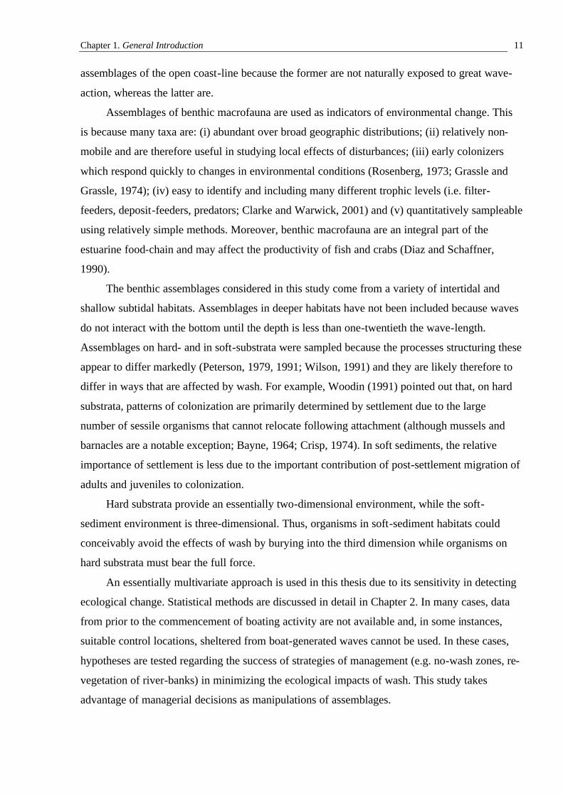
2.1 The Parramatta River
The Parramatta River (Fig. 2.1) is the largest river emptying into Port Jackson, Sydney,
Australia (151°13'E 33°52'S). It has a length of 19 km from its source in western Sydney to
Balmain, a width of 50-300 m and is up to 15 metres deep. The total area of the Parramatta River
catchment is 130 km2 and the waterway itself has an area of 12 km2 (NSW DLWC, 2000b). The
river is tidal to the Charles Street Weir in Parramatta, where it has a spring range that is 11%
greater than at the Heads (approximately 2.0 m).
About 85% of the Parramatta River catchment is urbanized (Total Environment Centre,
1996). Historically, the upper reaches have been subject to a lot of eutrophication and heavy
metal contamination due to the large number of industrial sites adjoining this section of river.
The situation has improved since the introduction of licensing procedures for trade waste in
1976, under the Clean Waters Act and Regulations (SPCC, 1987). A large proportion of the
catchment does, however, remain paved with impervious material or covered by buildings and
during periods of rain, large volumes of run-off containing garbage, soil, bacteria and dissolved
substances enter the river (Laxton, 1991).
The shores of the lower Parramatta River are dominated by hard substrata. Artificial
structures such as sandstone and concrete seawalls, pontoons and pilings are common as is
natural rocky reef, which is composed of Hawkesbury sandstone. Mangrove forests are reduced
to small remnant patches; sediment is generally coarse and sandy. To the west of Meadowbank,
there are large stretches of mangrove forest interspersed with unvegetated mudflat. The sediment
of the upper Parramatta River is much finer and contains greater proportions of clay and silt.
There has been extensive reclamation of land in the Homebush and Silverwater areas, with minor
reclamation in the majority of the other embayments along the river.
Along the Parramatta River, wind speed and direction vary locally according to topography and
distance from the sea. Winds may result from large-scale pressure patterns, nocturnal drainage
flows down slopes and valleys or from coastal systems. Winds arising from pressure patterns are
predominantly westerly from May to September and easterly from November to March. They are
strongest in September and weakest in April (Smith, 1990). Nocturnal winds (katabatic drift)
typically have speeds of less than 10km/h and are most frequent and of longest duration during
Figure 2.1 Map of the Sydney coastline showing the location of the Parramatta River. The inset shows the location of RiverCat wharves along
the river.
0 1 km
Botany Bay
Port Jackson
Hawkesbury River
0 2 0
K i l o m e t r e s
Sydney City
Drummoyne
DarlingHarbour
Circular QuayChiswick
Gladesville
AbbotsfordCabarita
Kissing Pt
Meadowbank
HomebushBay
Rydalmere
To Parramatta
0 1 2km
PARRAMATTA RIVER
Sydney

Chapter 2. RiverCats: Background and General Methods 16
winter (Hyde et al., 1983). Onshore sea breezes usually have speeds of less than 30 km/h and are
most prevalent during the afternoon and evening of the warmer months (Smith, 1990).
The Parramatta River is a popular location for recreational boating due to its proximity to
Sydney city. Boat traffic is greatest on the lower Parramatta River and decreases with distance
from Sydney Harbour (Patterson Britton, 2000b; Table 2.1). The majority of boating activity at
Silverwater can be attributed to the RiverCat ferries (70-74%, Table 2.1).
2.2 History of boating on the Parramatta River
Since European settlement, the Parramatta River has been an important transport link
between Sydney city and Parramatta. Initially, row-boats were used to transport goods between
the colony at Sydney Cove and the farming outpost of Rose Hill, but, in October, 1789, the first
ferry was commissioned (Andrews, 1975).
Only vessels of shallow draught, traveling at high tide, were able to navigate the last few
kilometres of channel to Parramatta. When deeper-draught, propeller-driven ferries replaced
paddle-wheelers in the late 1870s, the terminus had to be moved back to Duck Creek,
Silverwater, with passengers transported the remaining 4.5 km by steam tram (Andrews, 1975).
This change marked the beginning of the demise of the ferries. In 1928, services were cut back to
Gladesville and in the early 1950s, services ceased altogether as commuters turned to road and
rail (Prescott, 1984).
In 1987, ferries were re-introduced to the river between Meadowbank and Sydney.
Wharves were opened at Meadowbank, Abbotsford, Gladesville, Drummoyne, Hunters Hill,
Balmain, McMahon’s Point and Circular Quay (State Transit, 1993). This service proved popular
and it was proposed to extend the services to Raven Point/Putney Point, Cabarita Point and
Chiswick. In 1988, the State Government directed the (then) Urban Transport Authority to
facilitate the introduction of a high-speed ferry service linking Parramatta and Sydney (Smith,
1990).
There were two main criteria for the design of the ferries. First, the travel-time between
Parramatta and Sydney was required to be equivalent to or shorter than that along road and rail
links. This translates to an average speed of 21 knots. Second, the wash produced by the ferries
must not impact the natural habitats and artificial structures of the river (Smith, 1990).
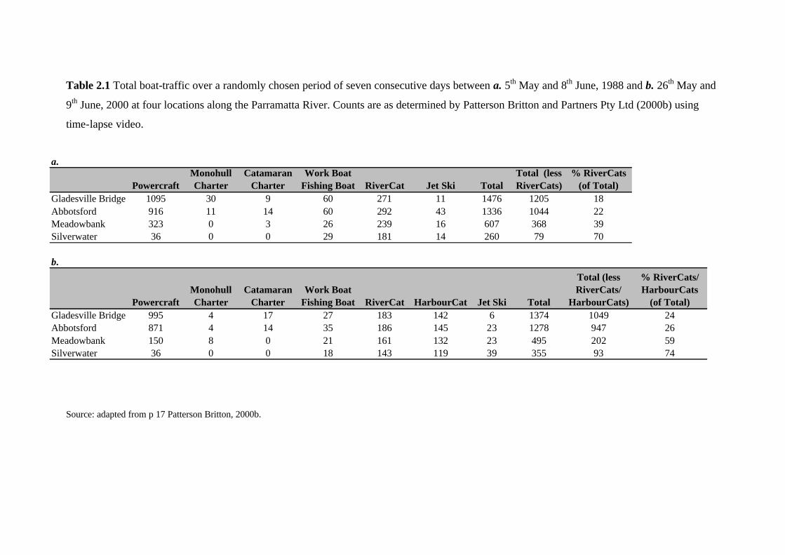
Table 2.1 Total boat-traffic over a randomly chosen period of seven consecutive days between a. 5th May and 8th June, 1988 and b. 26th May and
9th June, 2000 at four locations along the Parramatta River. Counts are as determined by Patterson Britton and Partners Pty Ltd (2000b) using
time-lapse video.
Source: adapted from p 17 Patterson Britton, 2000b.
a.
PowercraftMonohull Charter
Catamaran Charter
Work Boat Fishing Boat RiverCat Jet Ski Total
Total (less RiverCats)
% RiverCats (of Total)
Gladesville Bridge 1095 30 9 60 271 11 1476 1205 18Abbotsford 916 11 14 60 292 43 1336 1044 22Meadowbank 323 0 3 26 239 16 607 368 39Silverwater 36 0 0 29 181 14 260 79 70
b.
PowercraftMonohull Charter
Catamaran Charter
Work Boat Fishing Boat RiverCat HarbourCat Jet Ski Total
Total (less RiverCats/
HarbourCats)
% RiverCats/ HarbourCats
(of Total)Gladesville Bridge 995 4 17 27 183 142 6 1374 1049 24Abbotsford 871 4 14 35 186 145 23 1278 947 26Meadowbank 150 8 0 21 161 132 23 495 202 59Silverwater 36 0 0 18 143 119 39 355 93 74
Chapter 2. RiverCats: Background and General Methods 18
2.3 RiverCat ferries
Following a lengthy period of design and planning and the dredging of the upper reaches of
the river, the 35 m long, low-wash RiverCat ferries were introduced to the Parramatta River in
1993. To this date, these catamarans operate along a 24 km stretch of river between Circular
Quay and Parramatta (Fig. 2.1).
Despite being designed specifically for the Parramatta River, damage to the natural and
artificial structures of the river has been reported following their introduction. This includes
erosion and accretion of beaches, uprooting of mangroves and the collapse of seawalls (Wilson,
1994).
The wash produced by RiverCat ferries is of fairly small amplitude compared to the older
“Lady Class” ferries previously used on the Parramatta River. It has been proposed that the
deleterious effects of wash are due to “blockage” rather than the amplitude of the waves per se
(Patterson Britton, 2000c). Blockage results when vessels are operated in channels of restricted
width and/or depth. The effects of blockage include:
(i) surge – the rise in surrounding water-level preceding an approaching vessel;
(ii) draw-down – the lowering of the water level abreast of a passing vessel, often appearing as
a recession of water from a beach or bank as a vessel passes close offshore;
(iii) backwater flow – the acceleration of water across a shallow seabed as a vessel passes
above.
Blockage is typically a function of the dimensions of the channel, the dimensions of the vessel,
the vessel’s speed and the distance of the sailing-line from the shore (Dand, 1982).
Blockage and other effects of wash from RiverCat ferries are being considered in detail in a
long-term study of the shorelines of the Parramatta River commissioned by the NSW Waterways
Authority. This study, by Patterson Britton and Partners Pty Ltd, is on the effects of wash at four
sites along the upper Parramatta River between Rydalmere and Parramatta. These sites were
chosen because the river is very narrow at these places and the shoreline is particularly
susceptible to the effects of wash.
Results to date indicate that there is a critical speed of RiverCats at which erosion of
riverbanks occurs (Patterson Britton, 1999a). At Parramatta, this speed is 8-12 knots and at
Rydalmere it is 10-14 knots. These speeds are commonly associated with near-bed velocities of 1
m.s-1, although this varies with tide. Above the critical speed, vessels produce waves of reduced
height and shorter period. These can still cause significant increases in turbidity and bed
velocities of up to 0.7 m.s-1 from breaking on the shore.
Chapter 2. RiverCats: Background and General Methods 19
The observation of a non-linear relationship between speed of the ferries and near-bed flow
is as predicted from calculations of depth Froude (Fd) numbers (a unit-less number which relates
the velocity of a fluid to the velocity of waves in an open channel):
Fd = V.(gd)-0.5
where V is the speed of the vessel, g is the acceleration due to gravity and d is water-depth. At
relatively low values of Fd (0.6), wave heights are small and both transverse and divergent waves
are produced (Patterson Britton, 2000c). Surge and draw-down appear to peak at depth Froude
numbers around 0.7; at higher and lower depth Froude numbers they are negligible. As Fd
approaches 1.0, waves converge to form a single, large transverse wave. This may be followed
by a series of smaller waves of shorter period. The magnitude of the initial wave decreases
beyond depth Froude numbers of 1.0. As a general rule, depth Froude numbers in the range of
0.6 - 1.0 produce waves of greatest height and energy, so should be avoided by ferry captains
(Patterson Britton, 1999a).
2.4 Present strategies of management
A number of strategies of management have been adopted along the Parramatta River in
response to the perceived effects of RiverCat wash.
The first of these is the establishment of a no-wash zone on the upper Parramatta River,
between the Silverwater Bridge and the western terminus of services at Parramatta. Within this
zone, RiverCats are legally required to travel at speeds less than or equal to 7 knots (15 km/h).
Adherence to this regulation is sporadically monitored by NSW Waterways. There is another no-
wash zone along the Parramatta River, between the Gladesville Bridge and Five Dock Point,
which pre dates the RiverCat ferry service. Along other sections of the river, speed is
unrestricted and ferries commonly travel at up to 30 knots.
The second is the planting of mangrove seedlings along unvegetated river banks in an
attempt to stabilize the sediment and reduce erosion.
Finally, in 1998, two smaller HarbourCat ferries were added to the RiverCat fleet. These
are 24 m in length so should, presumably, cause less blockage than the larger RiverCat ferries.
Patterson Britton and Partners (1999b) have examined the relationship between the speed of
these vessels and depth Froude number, current-velocity and wave-height. Their results suggest
that there is a greater “buffer-zone” above the 7 knot speed limit for HarbourCat than RiverCat
ferries, before wash starts to affect deleteriously the river’s foreshores. The HarbourCats do,
Chapter 2. RiverCats: Background and General Methods 20
however, have a greater displacement-to-length ratio (2.5 x 10⁻³ tonnes.m-3) than do RiverCats
(1.4 x 10⁻³ tonnes.m-3; Patterson Britton, 2000c). This ratio is purportedly correlated with the
erosive capacity of wash (see Stumbo et al. 1999).
There is no distinction between RiverCats and HarbourCats on timetables for the ferry
service – they are used interchangeably. Thus, for the purposes of this thesis, RiverCats and
HarbourCats will be collectively referred to as RiverCat ferries.
2.5 General Methods
In the subsequent chapters, a number of experiments investigating the effects of wash from
RiverCat ferries on assemblages on hard- and in soft-substrata are described. Here, the general
methodology of these experiments is outlined.
All sampling of hard and soft substrata was done during low tide.
2.5.1 Sampling of hard substrata (seawalls)
To ensure that assemblages sampled on different seawalls could be compared, it was
necessary to sample them at the same tidal height. This was done by inserting screws into the
seawall at a single height and measuring the distance between these and the waterline at an
arbitrary level of the tide (as per Blockley, 1999; Chapman and Bulleri, 2003). The tidal height at
the time of measurement was obtained from Sydney Ports Corporation and the height of the
screws above MLWS thus calculated.
Two tidal heights were sampled. These are referred to as mid- and high-shore and were 0.9
m and 1.4 m above MLWS, respectively. It was not possible to sample any lower because of the
rubble adjacent to many of the seawalls that may shelter low-shore assemblages from the effects
of wash.
Sampling was done using quadrats (described in Section 3.2) placed on the seawall so that
their centre was at the required height. Abundances of algae and sessile animals were recorded as
percentage covers; mobile organisms were counted within the quadrats. Cover was recorded as
primary if the organism was directly attached to the substratum and secondary if it was attached
to the primary cover.
2.5.2 Soft sediment
Sampling of sediment and associated fauna was done using corers, 10 cm in diameter and
constructed of PVC pipe, following Morrisey et al. (1992). These were inserted into the sediment
to a depth of 10 cm and carefully dug out. Cores were emptied into individually labeled plastic
Chapter 2. RiverCats: Background and General Methods 21
bags and transported back to the laboratory, where they were either immediately preserved or
stored overnight at 4oC. Preservation was with 7% formalin in seawater. Animals were stained
using Biebrich Scarlet.
Samples were sieved through a 500 µm mesh. This size of mesh has been found to allow
accurate and cost-efficient sampling of spatial variation of assemblages of macrofauna in soft
sediments (Lewis and Stoner, 1981; Eleftheriou and Holme, 1984; Hartley and Dicks, 1987;
James et al., 1995). Animals retained on the sieve were kept for identification and enumeration.
In the case that the sediment was coarse and did not fall through the sieve, animals were
separated from the sediment by elutriating each core ten times. Before disposing of the sediment,
it was quickly checked under a hand-lens to ensure that all animals had been removed.
All fauna retained by the sieve were identified and counted under a dissecting microscope.
In the case of fragmented organisms, only anterior pieces (i.e. heads) were counted, so as not to
over-estimate their number. Where only the posterior end was present (i.e. no anterior end was
found for that taxon), the animal was given a count of one.
2.5.3 Taxonomic resolution
The analysis of assemblages is generally regarded as expensive due to the time involved in
identifying and sorting animals to the level of species (Clarke and Warwick, 2001). In places
such as Australia, this is not aided by the paucity of taxonomic information available and the
great uncertainty that may be associated with classification. The identification of organisms to
broader taxonomic groups (i.e. genus, family, phylum) saves time and money and, in most
instances, does not result in the significant loss of ecological information (e.g. James et al., 1995;
Chapman, 1998). The use of a coarser taxonomic resolution may, in fact, be more appropriate for
assessments of environmental impacts because natural variation at the level of species is often
great and may preclude detection of an impact (Clarke and Warwick, 2001).
The taxonomic resolution used in this study varied among types of fauna according to their
abundance, their morphological complexity and the taxonomic information available. In general,
groups of infauna were kept broad to minimize sorting time. For example, polychaetes were
sorted to family, crustaceans, in most cases, were sorted to order and bivalves and gastropods
were sorted to species.
Taxa comprising assemblages of hard substrata are generally much quicker and easier to
identify. In this study, they were identified to the finest taxonomic resolution possible, which
was usually species or genus.
Chapter 2. RiverCats: Background and General Methods 22
2.6 Analyses
This thesis uses a predominantly multivariate approach to assess the impact of boat-wash
on assemblages of benthic marine organisms. Univariate analyses were used to examine patterns
of abundance of individual taxa and environmental variables.
2.6.1 Multivariate analyses
A combination of measures of dissimilarity, ordination techniques and non-parametric
statistical analyses were used to examine differences in assemblages.
Unless otherwise indicated, all ordinations and analyses were done using Bray-Curtis
coefficients of dissimilarity (Bray and Curtis, 1957). This measure has been recommended for
ecological data because it takes the value 0 when two samples are identical and 100 when they
have no species in common, is independent of the scale of measurement, is not affected by joint
absences or the inclusion of additional samples within a matrix and registers differences in total
abundance of two samples as a less-than-perfect similarity, even when the relative abundances of
all species are identical (Clarke, 1993).
Unlike univariate analyses, some multivariate analyses do not require assumptions of
homogeneity of variances. In many multivariate analyses, the role of transformation is to down-
weight the contribution of common species so that the outcome is not overly dependent on
patterns in abundant species (Clarke, 1993; Clarke and Warwick, 2001). There does not,
however, appear to be any biological reason why less abundant taxa should be forced to
contribute relatively more to measures of dissimilarity than do more abundant taxa. Analyses of
untransformed data consequently formed the basis for the interpretation of experiments in this
thesis. These analyses took into consideration the species present, their frequencies of occurrence
in samples, their relative abundances and the total abundance of organisms within a sample (see
Tabachnick and Fidel, 1989).
Analyses were also done on presence-absence data to determine whether patterns evident in
the original data were driven by the species present in the samples or their abundances. Presence-
absence data has the effect of giving equal weight to all species, regardless of whether they are
rare or abundant. Presence-absence analyses are still, however, affected by frequency of
occurrence, which is often correlated with abundance.
Multivariate data were ordinated on two-dimensional plots using non-metric multi-
dimensional scaling (nMDS; Shephard, 1962; Kruskal, 1964). nMDS uses the rank order of
dissimilarity coefficients to produce a ‘map’ of the data. The distances between points on the
plot have the same rank order as the corresponding dissimilarities between samples - the closer
Chapter 2. RiverCats: Background and General Methods 23
together the points, the more similar the samples they represent. The extent to which the
representation agrees with the original data is reflected in its stress. A plot with a stress of less
than 0.1 is generally considered to be a good representation of the data and the risk of
misinterpretation is minimal. Plots with a stress of 0.1-0.2 are also potentially useful, but it is
recommended that any conclusions drawn from these be cross-checked with those from
alternative techniques (Field et al., 1982; Clarke, 1993).
Non-parametric multivariate analysis of variance (NP-MANOVA; Anderson, 2001) and
analysis of similarities (ANOSIM; Clarke, 1993) were used to test hypotheses about multivariate
differences among assemblages. Both methods were used to analyse data collected from simple,
mensurative experiments because NP-MANOVAs test hypotheses regarding multivariate
distances (measures of dissimilarity) whereas ANOSIMs test hypotheses regarding rank
dissimilarities. Data collected from more complex manipulative experiments were analysed
using NP-MANOVA only, because, unlike ANOSIM, it can be used to test for interactions. NP-
MANOVA compares within-group to between-group sums of squared dissimilarities, using a
permutation test to obtain a P-value.
ANOSIM is based on rank similarities between samples. Between-group ranks are
compared to the within-group ranks giving a test statistic, R. The test statistic may lie between 1
and –1 and is approximately zero when the null hypothesis is true. The statistical significance of
R-observed is determined by comparing it to the distribution of the R statistic obtained by
recalculating it under permutations of the sample labels. One of the limitations of ANOSIM is
that any samples that are totally devoid of animals must be removed from the data matrix before
the analysis can be done. While it may be argued that these samples are ecologically irrelevant
since they do not contain an assemblage, they may be important in the analysis of impacts that
decrease the types and numbers of organisms. This problem was eliminated by inserting a
dummy variable that had a uniform value across samples into the data matrix. This ensured that
all samples had at least one organism without interfering with measures of dissimilarity.
Each of these methods can only analyse a maximum of two factors at a time. Experimental
designs used in this thesis commonly had three factors – exposure (wash/no-wash), locations
within exposure groups and sites within locations. Consequently, the spatial scale of location was
often omitted from multivariate analyses so that patterns on the scale of exposure group and site
could be examined.
Unless otherwise indicated, the F-distributions of null hypotheses, tested using NP-
MANOVA, were calculated using 4999 permutations of residuals under the full model (ter
Braak, 1992, Anderson and Legendre, 1999). This type of permutation was used because: (i) the
Chapter 2. RiverCats: Background and General Methods 24
number of levels of nested factors was often sufficiently small to preclude a meaningful test if
restricted permutations of raw data (Anderson, 2001) were used and (ii) it can be used to rapidly
test orthogonal designs where the number of replicates is at least 5 (Anderson, 2001).
In the case that NP-MANOVA or ANOSIM detected a statistically significant difference (P
= 0.05) among levels of a term of interest, relevant a posteriori pair-wise comparisons were
done. Species contributing most to multivariate differences between samples were identified
using SIMPER (Clarke, 1993).
2.6.2 Univariate analyses
Multi-factorial analyses of variance (ANOVA) were used to test hypotheses concerning
differences in the abundance of individual taxa. Multivariate patterns may be explained by
several univariate patterns if a few species are controlling the structure of assemblages.
ANOVA assumes homogeneity of variance and this was tested for using Cochran’s C-test.
Many taxa of infauna from the Parramatta River had log-normal distributions and Cochran’s C-
test was consistently significant. These data were transformed using ln(x + 1) (see Underwood,
1997). In some analyses, heterogeneous variances could not be stabilised by transformation.
Given that analysis of variance is relatively robust to heterogeneous variances (Box 1953,
Underwood 1997), particularly if there are many independent estimates of variance, data were
analysed regardless. Significant results were interpreted with caution due to the increased
probability of Type I error associated with the analysis of such data.
Non-significant terms were pooled with the residual using the criterion P > 0.25 (Winer et
al., 1991) where this resulted in a more powerful test for the main effects of interest.
Analyses of variance were followed by a posteriori Student-Newman-Keul tests (SNK
tests) to identify significant differences among appropriate means (Winer et al., 1991;
Underwood, 1997).
CHAPTER 3
PATTERNS IN THE DISTRIBUTION AND ABUNDANCE OF INTERTIDAL ORGANISMS ON SEAWALLS SHELTERED FROM AND EXPOSED TO THE WASH OF RIVERCAT
FERRIES
3.1 Introduction
Wave-exposure along rocky shores is known to have direct effects on biota and to modify
ecological interactions (e.g. Dayton, 1975; Menge, 1978a; Seapy and Littler, 1978; Underwood,
1981; McQuaid and Branch, 1984; Underwood and Jernakoff, 1984; Bell and Denny, 1994; Viejo
et al., 1995). Intertidal assemblages exposed to great wave-energy may have an increased vertical
distribution of sessile organisms, such as barnacles (Seapy and Littler, 1978; Underwood, 1981;
McQuaid and Branch, 1985) and algae (Underwood and Jernakoff, 1984), a greater abundance of
macro-algae (Underwood, 1981; Underwood and Jernakoff, 1984, McQuaid and Branch, 1984,
1985; Bustamante and Branch, 1996) and filter-feeders (McQuaid and Branch, 1985), or a greater
total biomass (McQuaid and Branch, 1985; Ricciardi and Bourget, 1999) than assemblages on
sheltered shores. The species comprising intertidal assemblages may also differ between sheltered
and exposed shores. For example, on exposed shores, foliose algae may be replaced by calcareous
and leathery macrophytes (Phillips et al., 1997) or small, finely branched species (Kautsky and
Kautsky, 1989).
The effect of wave-action on intertidal organisms may be a result of wetting by wash or
splash, or a result of mechanical action due to the movement or energy of waves (see Southward,
1958; Jones and Demetropoulos, 1968). On wave-exposed shores, the wetting of the substratum
to a greater height may allow organisms which have upper vertical limits determined by physical
factors to occupy higher levels than they would in places sheltered from wave-action (e.g.
Underwood and Jernakoff, 1984). Such wetting may also increase the period over which a
substratum is immersed, potentially increasing the proportion of time during which planktonic
larvae can settle, filter-feeders can feed and wastes are released into the aquatic environment, but
potentially reducing the period over which algae can photosynthesise (see Menge, 1978a; Koehl,
1986). The mechanical action of waves results in greater friction and dynamic pressure on
organisms and may act to dislodge organisms from the substratum or result in changes to their
behaviour and morphology (Menge, 1974; Menge, 1978a,b; Denny et al., 1985; Brown and
Quinn, 1988; Trussel et al., 1993; Hobday, 1995; Etter, 1996; Blanchette, 1997). As most waves
break at low to mid-tidal heights, the mechanical action of waves should be greater at these than
Chapter 3. Patterns in the distribution and abundance of organisms on seawalls
26
at higher levels. Wetting by splash and spray may, however, affect all levels on the shore. Thus, it
may be hypothesised that the effect of wave-action on assemblages will differ among tidal heights.
A similar suite of species is found on seawalls as on rocky shores (Blockley, 1999; Chapman
and Bulleri, 2003). Patterns in the distribution and abundance of these species may therefore be
modified by similar processes on seawalls and rocky shores. Seawalls along the Parramatta River
are exposed to the wash of passing RiverCat ferries. While RiverCat wash is generally smaller
than the waves of the open coast, many of their effects, such as increasing the height to which the
substratum is wet, are analogous. If the ecology of seawalls is indeed modified by the same
processes as on rocky shores, the wash of RiverCat ferries should have a similar affect on the
intertidal assemblages of seawalls as oceanic waves have on intertidal assemblages on rocky
shores. If this model is correct, the distribution and abundance of organisms will differ between
seawalls that are exposed to and sheltered from wash.
RiverCats travel along the entire navigable length of the Parramatta River, making it
impossible to compare the assemblages on seawalls exposed to wash with those completely
sheltered from wash, without the possibility of confounding with other factors. Seawalls located
in large bays along the river, which are sheltered from the wash of RiverCat ferries, are also
sheltered from wind-waves and much of the wash produced by other commercial and recreational
vessels. They are also likely to be subject to different small-scale hydrodynamic processes because
they are at the heads of bays. Sandstone seawalls, of similar construction to those along the
Parramatta River are absent from adjacent estuaries (i.e. Georges River, Port Hacking and
Pittwater). A comparison may, however, be made between seawalls along the Parramatta River
that are more or less exposed to the wash of RiverCat ferries.
The energy and height of boat-generated waves decreases with distance from the sailing line
(Das and Johnson, 1970; Bhowmik, 1975). Thus, seawalls located closer to the main RiverCat
ferry route (on points) should be more exposed to the wash of RiverCat ferries than those located
further away (in small bays along the main river channel).
In this chapter, two hypotheses were tested: (i) assemblages found at mid- or high tidal
heights on seawalls close to the RiverCat ferry route will differ from those on seawalls further
away and (ii) the mean maximal height at which barnacles or algae are found will be greater on
seawalls close to the ferry route than on those further away. These hypotheses are very general
because the structure of assemblages on seawalls along the Parramatta River had not previously
been determined and more specific predictions about the effect of wave-action could not therefore
Chapter 3. Patterns in the distribution and abundance of organisms on seawalls
27
be made. During sampling, however, more observations were made, more specific models
developed and tests of the corresponding hypotheses described.
3.2 Materials and Methods
In order to test the hypothesis that the assemblages found on seawalls close to the RiverCat
ferry route will differ from those found on seawalls further away, vertical sandstone seawalls were
sampled at two locations close to the ferry route (Abbotsford Point [N1] and Henley [N2]) and
two locations further from the ferry route (Looking Glass Bay [F1] and Abbotsford Bay [F2]) on
the 19th and 20th May, 2000 (Figure 3.1). At each location, two 5 m-long sections of wall were
haphazardly selected as sites. These were separated by at least 5 m so that spatial independence of
sampling would be maintained. Estimates of the abundance of species were determined using 25
points of intersection of a 15 x 15 cm quadrat strung with a grid of nylon strings at 2.5 cm
intervals. Five quadrats were randomly placed at mid- and high tidal heights (see Section 2.5.1)
and the abundance of all sessile and mobile species in each quadrat was determined using the
method described in Section 2.5.1. This size of quadrat was chosen so that less than 16 % of the
total area of the sites would be sampled at any one time and sampling could consequently be
temporally independent (see Banwell, 1996).
The maximal height above MLWS at which (i) barnacles and (ii) algae were found was also
determined at 10 places within each site to test the hypotheses that the maximal height at which
barnacles or algae would be found will be greater on seawalls close to the RiverCat ferry route
than on walls further away. Ten horizontal distances along the wall were selected using random
numbers. At each horizontal distance, the maximal height above MLWS at which barnacles or
algae were found was recorded. Heights were measured relative to points of known elevation.
During this initial sampling, the observation was made that seawalls orientated perpendicular
to the direction of propagation of waves appeared more exposed to the wash of RiverCat ferries
than seawalls orientated parallel to the direction of propagation. The abundance of macro-algae
and the cover of Mytilus sp. were greater on seawalls exposed to the wash of RiverCat ferries
than on walls sheltered from wash, while the abundance of the barnacle, Hexaminius foliorum,
showed the opposite pattern. The mussel, Xenostrobus securis, was only found in areas that were
most sheltered from wash (i.e. further from the RiverCat ferry route).
It was hence predicted that further sampling of seawalls close to or further from the
RiverCat ferry route and oriented perpendicular or parallel to the direction of propagation of wash
would find that:
Chapter 3. Patterns in the distribution and abundance of organisms on seawalls
28
1. Walls located close to the RiverCat ferry route and orientated perpendicular to the
direction of propagation of wash would be the most exposed and walls located further
from the RiverCat route and parallel to the direction of propagation of waves the least
exposed to the wash of RiverCat ferries.
2. The total cover of algae would be greater on seawalls close to the RiverCat ferry route
than on seawalls further away and would be greater on seawalls orientated perpendicular
to the direction of propagation of wash than on those orientated parallel.
3. The abundance of Mytilus sp. would follow the patterns described above for algae.
4. The percentage cover of H. foliorum would be less on seawalls close to the ferry route
than on those further away and on walls perpendicular to the direction of propagation of
waves than those that are parallel.
5. X. securis would only be present on sheltered seawalls (i.e. those that are further from
the RiverCat ferry route and are orientated perpendicular to incoming wash).
In order to test these hypotheses, seawalls close to the ferry route and orientated perpendicular to
the direction of propagation of wash (Abbotsford Point, Henley, Parramatta River Sailing Club),
close to the ferry route and parallel to incoming wash (Abbotsford Point, Bedlam Bay 1, Bedlam
Bay 2), further from the ferry route and perpendicular to wash (Abbotsford Bay, Gladesville
Hospital, Putney Park) and further from the ferry route and parallel to wash (Abbotsford Bay,
Looking Glass Bay and Putney Park) were sampled on the 9th and 10th August, 2000 (Fig. 3.2).
Only one 5 m-long site was sampled on each wall due to the limited length of wall with the
required orientation. As with the initial sampling, five 15 x 15 cm quadrats were randomly
positioned at each tidal height and the abundances of macro-algae, H. foliorum, Mytilus sp. and
X. securis determined.
The upper limits of (i) algae and (ii) barnacles were also determined at ten positions within
each site at this second time of sampling, using the same method outlined above. This was to test
the hypothesis that the mean maximal vertical height of each will be greater on exposed seawalls
(located close to the ferry route and orientated perpendicular to incoming wash) than on sheltered
walls (located further from the ferry route and parallel to incoming wash).
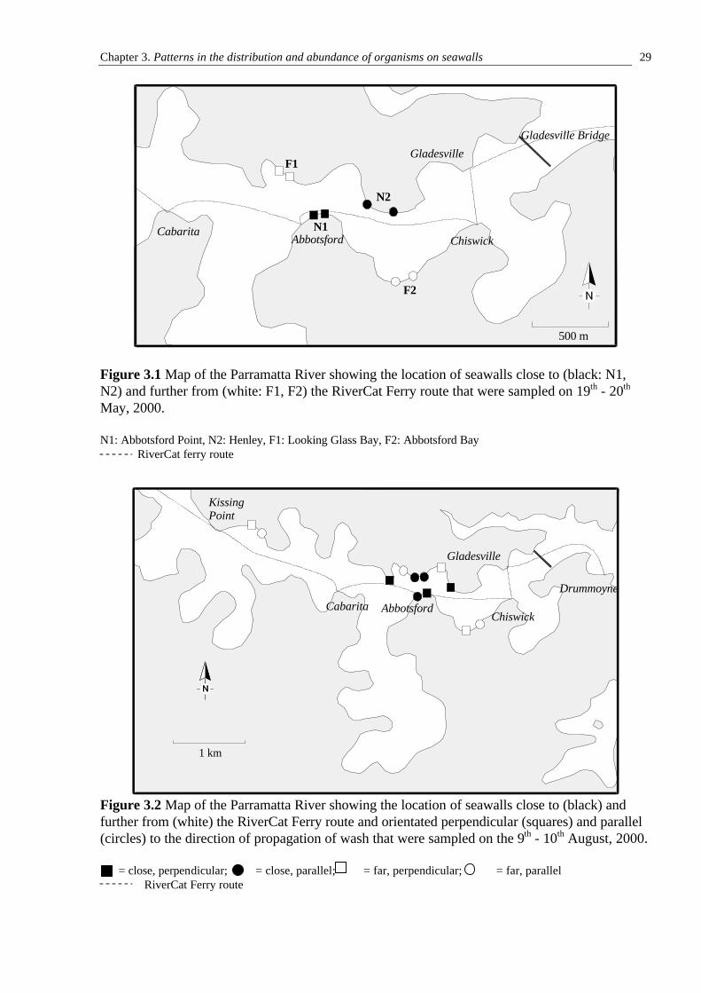
Chapter 3. Patterns in the distribution and abundance of organisms on seawalls
29
Figure 3.1 Map of the Parramatta River showing the location of seawalls close to (black: N1, N2) and further from (white: F1, F2) the RiverCat Ferry route that were sampled on 19th - 20th May, 2000. N1: Abbotsford Point, N2: Henley, F1: Looking Glass Bay, F2: Abbotsford Bay RiverCat ferry route
Figure 3.2 Map of the Parramatta River showing the location of seawalls close to (black) and further from (white) the RiverCat Ferry route and orientated perpendicular (squares) and parallel (circles) to the direction of propagation of wash that were sampled on the 9th - 10th August, 2000. = close, perpendicular; = close, parallel; = far, perpendicular; = far, parallel RiverCat Ferry route
Abbotsford
Gladesville
ChiswickCabarita
Gladesville Bridge
500 m
N1
N2
F1
F2
1 km
Cabarita AbbotsfordChiswick
Gladesville
KissingPoint
Drummoyne
Chapter 3. Patterns in the distribution and abundance of organisms on seawalls
30
Differences between assemblages on seawalls close to or further from the RiverCat ferry
route were examined using nMDS ordinations of centroids representing sites and NP-MANOVA
(Anderson, 2001) and ANOSIM (Clarke, 1993) of untransformed data and measures of presence-
absence. Data for mid- and high tidal heights were analysed separately because assemblages differ
markedly between these. Only the factors, proximity and sites, were analysed because NP-
MANOVA and ANOSIM can only handle two factors at a time (see Section 2.6.1). The factor
location was omitted because spatial variability was greater at the scale of sites. Centroids were
used in nMDS ordinations because of the large stress of plots using individual quadrats. Both NP-
MANOVAs and ANOSIMs were done because they use different methods to calculate test
statistics and therefore test different hypotheses (see Section 2.6.1). Both untransformed and
presence-absence data were analysed because a comparison of their results enable separation of
the contribution of differences in the abundances of species and differences in the types of species
present in determining patterns. Any difference found when untransformed data is analysed may
be due to differences in the species present, their abundance and frequency among replicates.
Analysis of presence-absence data does not consider abundances.
SIMPER (Clarke, 1993) analyses were done to identify the species contributing most to
differences between treatments. Differences in the abundance of these species between treatments
were then tested for using ANOVAs (see Section 2.6.6).
3.3 Results
Sixteen taxa of algae and 15 taxa of invertebrates were identified during this study (Table
3.1). Many algae were only identified to genus because of the similar appearance of individual
species in the field. In some cases, where algae were very small or present in complex mats, they
could not be assigned to a genus and were classified as green filaments or green film. “Scuzz”
refers to a brown scum found on surfaces; it may have been composed of detritus and/or a micro-
algal film.
3.3.1 Initial sampling of assemblages on seawalls close to or further from the RiverCat ferry
route
At a mid-tidal height, assemblages differed between seawalls close to or further from the
RiverCat ferry route. This was evident by a separation of centroids into two groups
corresponding to these proximities on nMDS plots of untransformed (Fig. 3.3(i)a) and presence-
absence (Fig. 3.3(ii)a) data. The analysis of untransformed data using NP-MANOVA and
Chapter 3. Patterns in the distribution and abundance of organisms on seawalls
31
ANOSIM showed the difference between treatments (proximity to wash) to be statistically
significant (p < 0.05, Tables 3.2a, 3.3a). An ANOSIM using the presence-absence data did not,
however, find any significant difference between the two groups (p > 0.05, Table 3.3a) despite the
significant result of the NP-MANOVA (p < 0.05, Table 3.2a). Given the small number of possible
permutations (35) that could be used for the ANOSIM and the small significance level (6 %)
obtained for the test, it is, however, safe to consider the composition of assemblages different
between walls close to or further from the RiverCat route.
At the higher tidal level, the assemblage found in one of the sites at Henley appeared
considerably different from the other assemblages (Fig. 3.3(i)b). This appeared to be due to
greater abundance of the encrusting alga, Hildenbrandia rubra, at this site than at other places.
The ordination was repeated without this site in order to determine whether any pattern was
evident among the remainder of sites. No separation of points into ‘near’ and ‘far’ treatments was
evident (Fig 3.3(i)c) and no significant difference was found between these two treatments using
either NP-MANOVA (p > 0.05, Table 3.2b) or ANOSIM (p > 0.05, Table 3.3b). In contrast,
centroids of presence-absence data appeared to separate into ‘near’ and ‘far’ groups on nMDS
plots including or excluding the site at Henley (Fig. 3.3(ii)b,c). These differences were, however,
non-significant for untransformed and for presence-absence data using NP-MANOVA (p > 0.05,
Table 3.2b) and ANOSIM (p > 0.05, Table 3.3b).
Significant spatial variability was found among assemblages at the scale of sites at each of
the heights when untransformed or presence-absence data were analysed using NP-MANOVA (p
< 0.001, Table 3.2a,b). At the mid tidal height, Bray-Curtis measures of dissimilarity were larger
between sites of the ‘near’ proximity treatment than between sites of the ‘far’ treatment (Fig. 3.4,
Table 3.4). At the high tidal height, the opposite pattern was seen – assemblages were more
similar between sites near to the ferry route than between those further away (Fig. 3.4, Table 3.4).
No pattern was seen in measures of within-site variability between places near and far from the
ferry route (Fig. 3.5, Table 3.5) at either tidal height.
Many species contributed to the dissimilarity between the assemblages on seawalls close to
or further from the Rivercat route at the mid-tidal height (Table 3.6). In all cases, however, the
contribution of these species to the dissimilarity between treatments was no greater than their
contribution to among-site differences in one or more of the treatments. Based on these results, it
could not be concluded that any of the species were more important than the others in
contributing to the difference between the treatments.
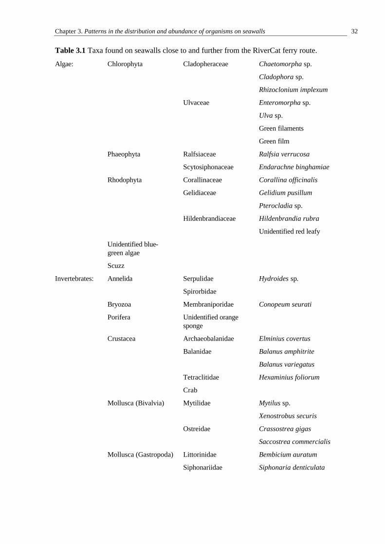
Chapter 3. Patterns in the distribution and abundance of organisms on seawalls
32
Table 3.1 Taxa found on seawalls close to and further from the RiverCat ferry route.
Algae: Chlorophyta Cladopheraceae Chaetomorpha sp.
Cladophora sp.
Rhizoclonium implexum
Ulvaceae Enteromorpha sp.
Ulva sp.
Green filaments
Green film
Phaeophyta Ralfsiaceae Ralfsia verrucosa
Scytosiphonaceae Endarachne binghamiae
Rhodophyta Corallinaceae Corallina officinalis
Gelidiaceae Gelidium pusillum
Pterocladia sp.
Hildenbrandiaceae Hildenbrandia rubra
Unidentified red leafy
Unidentified blue- green algae
Scuzz
Invertebrates: Annelida Serpulidae Hydroides sp.
Spirorbidae
Bryozoa Membraniporidae Conopeum seurati
Porifera Unidentified orange sponge
Crustacea Archaeobalanidae Elminius covertus
Balanidae Balanus amphitrite
Balanus variegatus
Tetraclitidae Hexaminius foliorum
Crab
Mollusca (Bivalvia) Mytilidae Mytilus sp.
Xenostrobus securis
Ostreidae Crassostrea gigas
Saccostrea commercialis
Mollusca (Gastropoda) Littorinidae Bembicium auratum
Siphonariidae Siphonaria denticulata
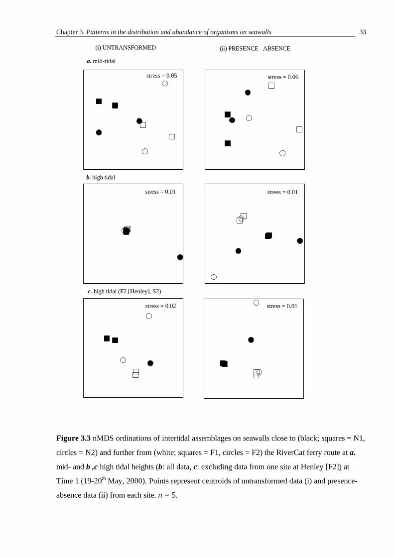
Chapter 3. Patterns in the distribution and abundance of organisms on seawalls
33
Figure 3.3 nMDS ordinations of intertidal assemblages on seawalls close to (black; squares = N1,
circles = N2) and further from (white; squares = F1, circles = F2) the RiverCat ferry route at a.
mid- and b ,c high tidal heights (b: all data, c: excluding data from one site at Henley [F2]) at
Time 1 (19-20th May, 2000). Points represent centroids of untransformed data (i) and presence-
absence data (ii) from each site. n = 5.
a. mid-tidal
stress = 0.05 stress = 0.06
stress = 0.01 stress = 0.01
b. high tidal
stress = 0.02 stress = 0.01
(i) UNTRANSFORMED (ii) PRESENCE - ABSENCE
c. high tidal (F2 [Henley], S2)
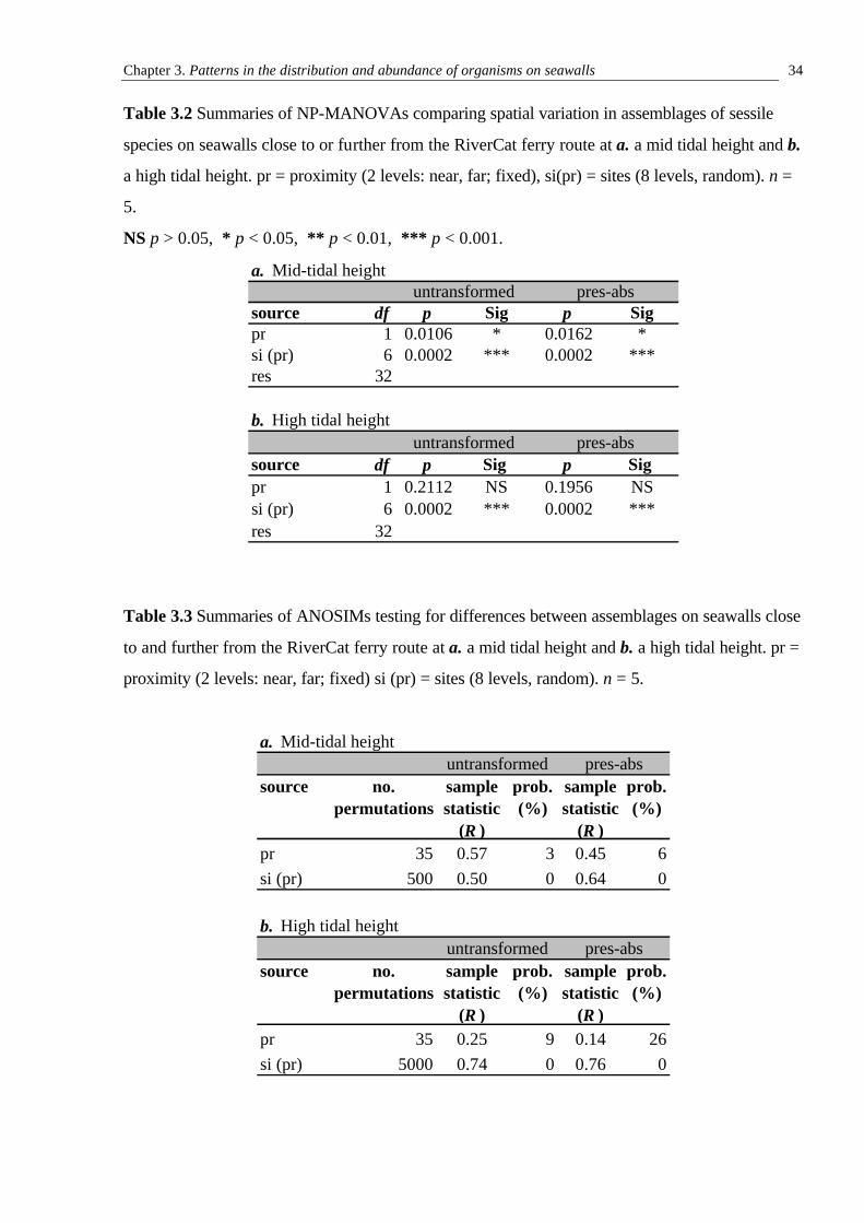
Chapter 3. Patterns in the distribution and abundance of organisms on seawalls
34
Table 3.2 Summaries of NP-MANOVAs comparing spatial variation in assemblages of sessile
species on seawalls close to or further from the RiverCat ferry route at a. a mid tidal height and b.
a high tidal height. pr = proximity (2 levels: near, far; fixed), si(pr) = sites (8 levels, random). n =
5.
NS p > 0.05, * p < 0.05, ** p < 0.01, *** p < 0.001.
Table 3.3 Summaries of ANOSIMs testing for differences between assemblages on seawalls close
to and further from the RiverCat ferry route at a. a mid tidal height and b. a high tidal height. pr =
proximity (2 levels: near, far; fixed) si (pr) = sites (8 levels, random). n = 5.
a. Mid-tidal height
source df p Sig p Sigpr 1 0.0106 * 0.0162 *si (pr) 6 0.0002 *** 0.0002 ***res 32
b. High tidal height
source df p Sig p Sig pr 1 0.2112 NS 0.1956 NSsi (pr) 6 0.0002 *** 0.0002 ***res 32
untransformed pres-abs
untransformed pres-abs
a. Mid-tidal height
source no. permutations
sample statistic
(R )
prob. (%)
sample statistic
(R )
prob. (%)
pr 35 0.57 3 0.45 6si (pr) 500 0.50 0 0.64 0
b. High tidal height
source no. permutations
sample statistic
(R )
prob. (%)
sample statistic
(R )
prob. (%)
pr 35 0.25 9 0.14 26si (pr) 5000 0.74 0 0.76 0
untransformed pres-abs
untransformed pres-abs
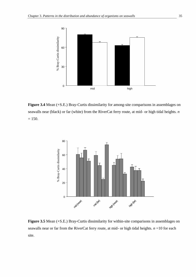
Chapter 3. Patterns in the distribution and abundance of organisms on seawalls
35
mid (ne
ar)
mid (fa
r)
high (
near)
high (
far)
0
20
40
60
80
% B
ray-
Cur
tis d
issi
mila
rity
Figure 3.4 Mean (+S.E.) Bray-Curtis dissimilarity for among-site comparisons in assemblages on
seawalls near (black) or far (white) from the RiverCat ferry route, at mid- or high tidal heights. n
= 150.
Figure 3.5 Mean (+S.E.) Bray-Curtis dissimilarity for within-site comparisons in assemblages on
seawalls near or far from the RiverCat ferry route, at mid- or high tidal heights. n =10 for each
site.
mid high0
30
60
90
% B
ray-
Cur
tis d
issi
mila
rity
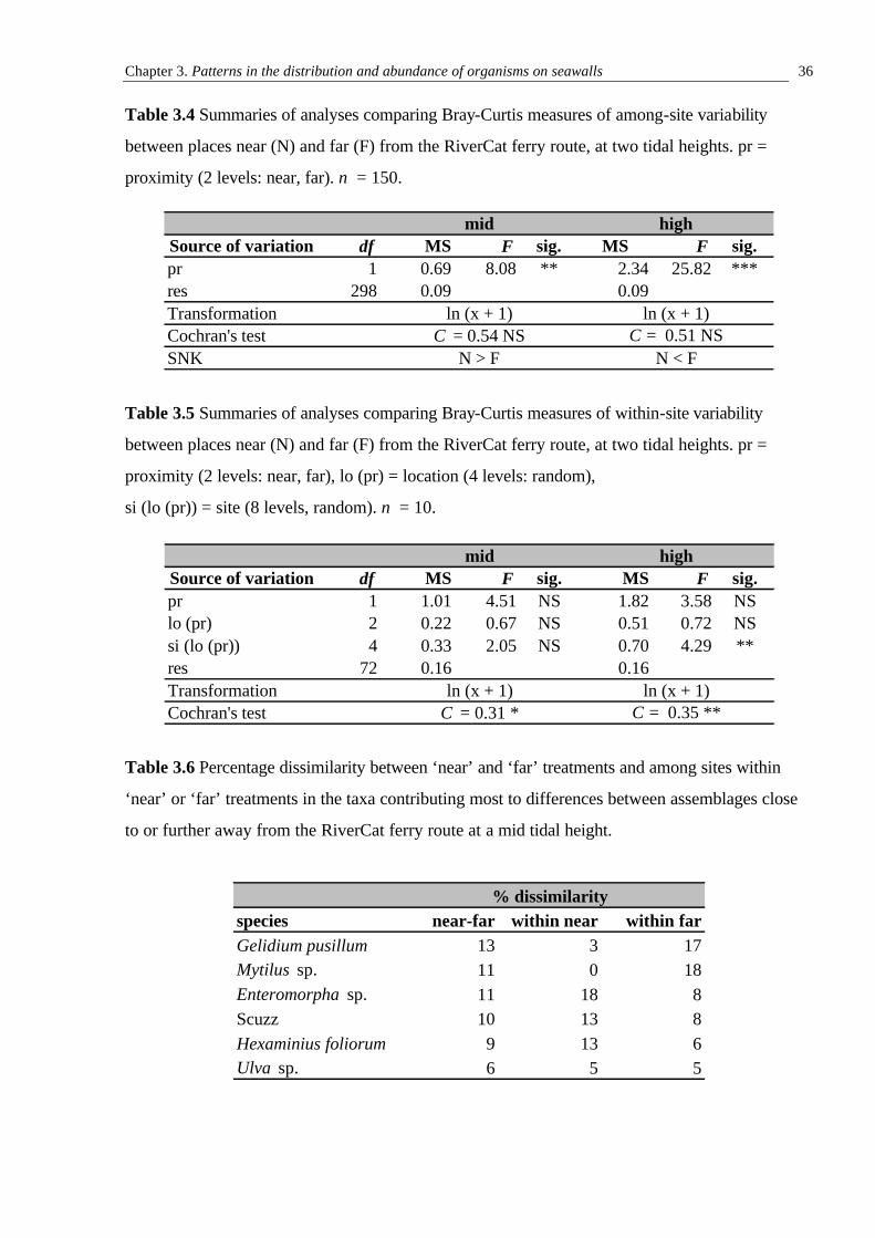
Chapter 3. Patterns in the distribution and abundance of organisms on seawalls
36
Table 3.4 Summaries of analyses comparing Bray-Curtis measures of among-site variability
between places near (N) and far (F) from the RiverCat ferry route, at two tidal heights. pr =
proximity (2 levels: near, far). n = 150.
Table 3.5 Summaries of analyses comparing Bray-Curtis measures of within-site variability
between places near (N) and far (F) from the RiverCat ferry route, at two tidal heights. pr =
proximity (2 levels: near, far), lo (pr) = location (4 levels: random),
si (lo (pr)) = site (8 levels, random). n = 10.
Table 3.6 Percentage dissimilarity between ‘near’ and ‘far’ treatments and among sites within
‘near’ or ‘far’ treatments in the taxa contributing most to differences between assemblages close
to or further away from the RiverCat ferry route at a mid tidal height.
highSource of variation df MS F sig. MS F sig.pr 1 0.69 8.08 ** 2.34 25.82 ***res 298 0.09 0.09TransformationCochran's test C = 0.51 NSSNK N > F N < F
mid
C = 0.54 NSln (x + 1) ln (x + 1)
highSource of variation df MS F sig. MS F sig.pr 1 1.01 4.51 NS 1.82 3.58 NSlo (pr) 2 0.22 0.67 NS 0.51 0.72 NSsi (lo (pr)) 4 0.33 2.05 NS 0.70 4.29 **res 72 0.16 0.16TransformationCochran's test C = 0.35 **
mid
C = 0.31 *ln (x + 1) ln (x + 1)
% dissimilarityspecies near-far within near within farGelidium pusillum 13 3 17Mytilus sp. 11 0 18Enteromorpha sp. 11 18 8Scuzz 10 13 8Hexaminius foliorum 9 13 6Ulva sp. 6 5 5
Chapter 3. Patterns in the distribution and abundance of organisms on seawalls
37
Univariate analyses were done on individual taxa to test the hypothesis that abundances of
these would differ between seawalls close to or further from the RiverCat ferry route. All species
that appeared to be present in a majority of quadrats within at least one of the two treatments
were analysed. Rare or very patchy species were not examined. Species fulfilling this criterion
were Enteromorpha sp., Ulva sp., Gelidium pusillum , Balanus amphitrite and Hexaminius
foliorum at both heights, Mytilus sp. at the mid-tidal height and Eliminius covertus at the high
tidal height. Univariate analyses were also done on the total abundances of macro-algae and
barnacles because previous studies suggested that the effects of wave-action on species were
consistent across these broad taxonomic groups (e.g. Seapy and Littler, 1978; Underwood, 1981;
Underwood and Jernakoff, 1984).
At the mid-tidal height, the mean abundances of Ulva sp., G. pusillum and Mytilus sp. were
significantly greater in sites close to the RiverCat ferry route than in sites further away (p < 0.05,
Table 3.7a, Fig. 3.6b,c,h). No significant difference between the two treatments was found in the
mean abundances of Enteromorpha sp. or B. amphitrite (p > 0.05, Table 3.7a, Fig. 3.6a,e). The
total abundance of algae appeared greater close to the ferry route than further away (Fig. 3.6d)
and the abundance of H. foliorum and the total cover of barnacles appeared greater in sites further
from the ferry route (Fig. 3.6f,g). These differences were, however, not statistically significant
because of the large variability found among sites in each treatment (p > 0.05, Table 3.7a).
At the high tidal height, a statistically significant difference was found between proximity-
treatments in the abundance of total macro-algae only (near > far, p < 0.05, Table 3.7b; Fig 3.7d).
The abundances of Ulva sp. and G. pusillum were greater on seawalls close to the ferry route
(Fig. 3.7b,c) and the abundance of E. covertus were greater on seawalls further away (Fig 3.7e).
These differences were, however, not statistically significant (Table 3.7b).
The lack of statistically significant results can be attributed to the great spatial variability of
abundances from site to site with proximity-treatments for almost all taxa (Table 3.7a,b).
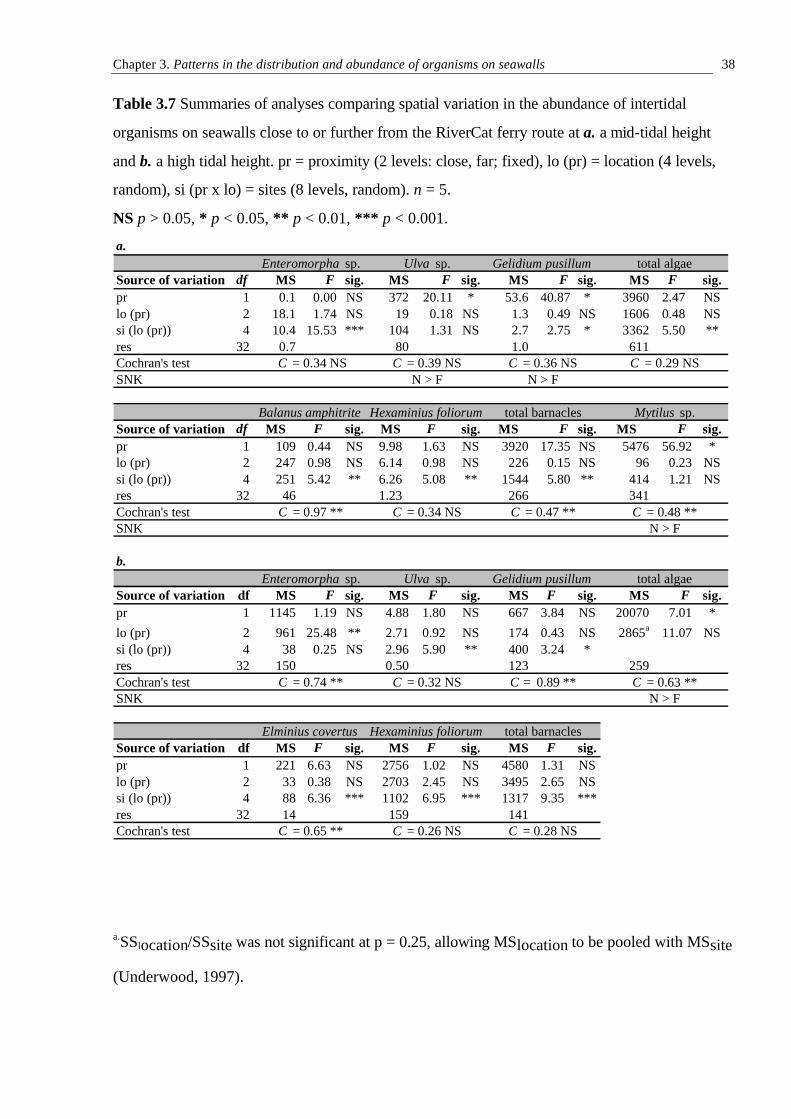
Chapter 3. Patterns in the distribution and abundance of organisms on seawalls
38
Table 3.7 Summaries of analyses comparing spatial variation in the abundance of intertidal
organisms on seawalls close to or further from the RiverCat ferry route at a. a mid-tidal height
and b. a high tidal height. pr = proximity (2 levels: close, far; fixed), lo (pr) = location (4 levels,
random), si (pr x lo) = sites (8 levels, random). n = 5.
NS p > 0.05, * p < 0.05, ** p < 0.01, *** p < 0.001.
a.SSlocation/SSsite was not significant at p = 0.25, allowing MSlocation to be pooled with MSsite
(Underwood, 1997).
a.Ulva sp. Gelidium pusillum total algae
Source of variation df MS F sig. MS F sig. MS F sig. MS F sig.pr 1 0.1 0.00 NS 372 20.11 * 53.6 40.87 * 3960 2.47 NSlo (pr) 2 18.1 1.74 NS 19 0.18 NS 1.3 0.49 NS 1606 0.48 NSsi (lo (pr)) 4 10.4 15.53 *** 104 1.31 NS 2.7 2.75 * 3362 5.50 **res 32 0.7 80 1.0 611Cochran's test C = 0.34 NS C = 0.39 NS C = 0.36 NS C = 0.29 NSSNK N > F
Balanus amphitrite Hexaminius foliorum total barnacles Mytilus sp.Source of variation df MS F sig. MS F sig. MS F sig. MS F sig.pr 1 109 0.44 NS 9.98 1.63 NS 3920 17.35 NS 5476 56.92 *lo (pr) 2 247 0.98 NS 6.14 0.98 NS 226 0.15 NS 96 0.23 NSsi (lo (pr)) 4 251 5.42 ** 6.26 5.08 ** 1544 5.80 ** 414 1.21 NSres 32 46 1.23 266 341Cochran's test C = 0.97 ** C = 0.34 NS C = 0.47 **SNK N > F
b.Ulva sp. Gelidium pusillum total algae
Source of variation df MS F sig. MS F sig. MS F sig. MS F sig.pr 1 1145 1.19 NS 4.88 1.80 NS 667 3.84 NS 20070 7.01 *lo (pr) 2 961 25.48 ** 2.71 0.92 NS 174 0.43 NS 2865a 11.07 NSsi (lo (pr)) 4 38 0.25 NS 2.96 5.90 ** 400 3.24 *res 32 150 0.50 123 259Cochran's test C = 0.74 ** C = 0.32 NS C = 0.89 ** C = 0.63 **SNK N > F
Elminius covertus Hexaminius foliorum total barnaclesSource of variation df MS F sig. MS F sig. MS F sig.pr 1 221 6.63 NS 2756 1.02 NS 4580 1.31 NSlo (pr) 2 33 0.38 NS 2703 2.45 NS 3495 2.65 NSsi (lo (pr)) 4 88 6.36 *** 1102 6.95 *** 1317 9.35 ***res 32 14 159 141Cochran's test C = 0.65 ** C = 0.26 NS C = 0.28 NS
Enteromorpha sp.
Enteromorpha sp.
C = 0.48 **
N > F
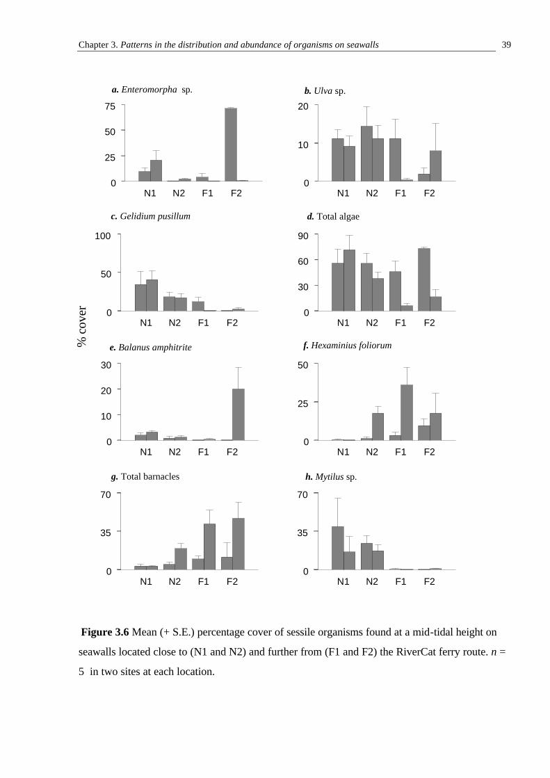
Chapter 3. Patterns in the distribution and abundance of organisms on seawalls
39
Figure 3.6 Mean (+ S.E.) percentage cover of sessile organisms found at a mid-tidal height on
seawalls located close to (N1 and N2) and further from (F1 and F2) the RiverCat ferry route. n =
5 in two sites at each location.
N1 N2 F1 F20
25
50
75
N1 N2 F1 F20
10
20
b. Ulva sp.
N1 N2 F1 F20
50
100
N1 N2 F1 F20
30
60
90
N1 N2 F1 F20
10
20
30
e. Balanus amphitrite
N1 N2 F1 F20
25
50
f. Hexaminius foliorum
N1 N2 F1 F20
35
70
N1 N2 F1 F20
35
70
h. Mytilus sp.
a. Enteromorpha sp.
c. Gelidium pusillum d. Total algae
g. Total barnacles
% c
over
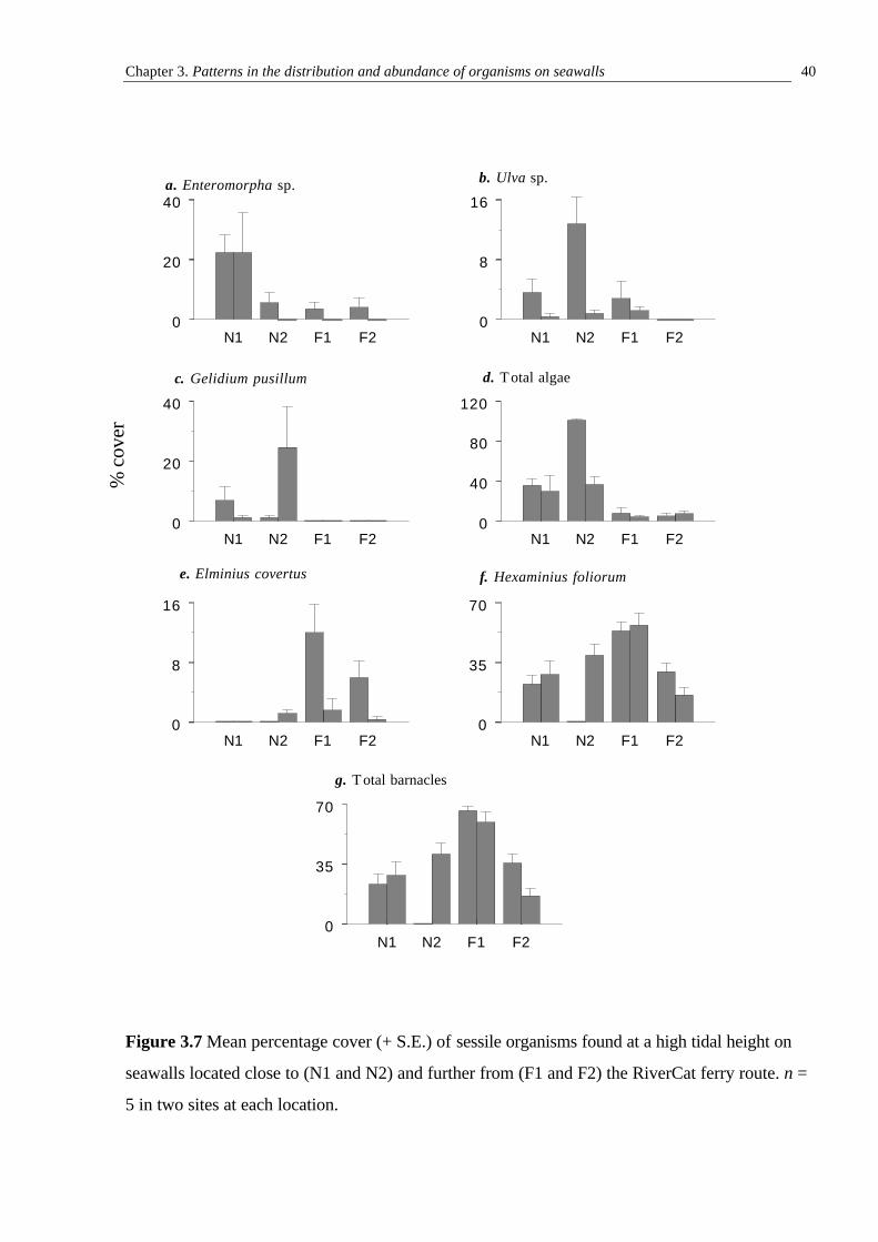
Chapter 3. Patterns in the distribution and abundance of organisms on seawalls
40
Figure 3.7 Mean percentage cover (+ S.E.) of sessile organisms found at a high tidal height on
seawalls located close to (N1 and N2) and further from (F1 and F2) the RiverCat ferry route. n =
5 in two sites at each location.
N1 N2 F1 F20
20
40a. Enteromorpha sp.
N1 N2 F1 F20
8
16
N1 N2 F1 F20
20
40
c. Gelidium pusillum
N1 N2 F1 F20
40
80
120
N1 N2 F1 F20
8
16
N1 N2 F1 F20
35
70
e. Elminius covertus f. Hexaminius foliorum
N1 N2 F1 F20
35
70
b. Ulva sp.
d. T otal algae
g. T otal barnacles
% c
over
Chapter 3. Patterns in the distribution and abundance of organisms on seawalls
41
3.3.2 Abundances of organisms on seawalls close to or further from the RiverCat ferry
route and orientated perpendicular and parallel to the direction of propagation of wash.
No significant difference was found in the abundance of macro-algae, H. foliorum or X.
securis between proximity or orientation treatments on seawalls at either high or mid tidal heights
(p > 0.05, Table 3.8a,b; Fig. 3.8a,b; Fig. 3.9a,b). At the mid-tidal height, however, X. securis was
only found on the most sheltered seawalls sampled (i.e. those further from the ferry route and
orientated parallel to the direction of propagation of wash, Fig. 3.8d), as predicted. A significant
proximity by orientation interaction was found in the cover of Mytilus sp. at the mid-tidal height
(p < 0.01, Table 3.8a, Fig 3.8c). Post-hoc SNK tests showed this interaction to be due to a
greater cover of Mytilus sp. on seawalls close to the ferry route and orientated perpendicular to
the direction of propagation of wash than on seawalls close to the ferry route but orientated
parallel to wash or on seawalls located further away. At the higher level, no pattern was found
between treatments in cover of this species (Table 3.8b, Fig. 3.9c).
3.3.3 The vertical distribution of sessile organisms on seawalls exposed to and more
sheltered from ferry wash
No pattern was found in the mean height of the upper limit of barnacles or algae on seawalls
exposed to and more sheltered from wash at either time of sampling (p > 0.05, Table 3.9a,b, Fig.
3.10, 3.11).
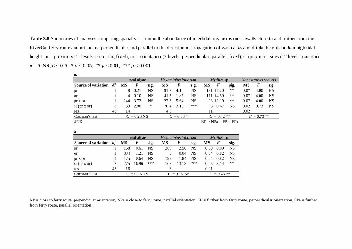
Table 3.8 Summaries of analyses comparing spatial variation in the abundance of intertidal organisms on seawalls close to and further from the
RiverCat ferry route and orientated perpendicular and parallel to the direction of propagation of wash at a. a mid-tidal height and b. a high tidal
height. pr = proximity (2 levels: close, far; fixed), or = orientation (2 levels: perpendicular, parallel; fixed), si (pr x or) = sites (12 levels, random).
n = 5. NS p > 0.05, * p < 0.05, ** p < 0.01, *** p < 0.001.
NP = close to ferry route, perpendicuar orientation, NPa = close to ferry route, parallel orientation, FP = further from ferry route, perpendicular orientation, FPa = further from ferry route, parallel orientation
a.total algae Hexaminius foliorum Mytilus sp. Xenostrobus securis
Source of variation df MS F sig. MS F sig. MS F sig. MS F sig.pr 1 8 0.21 NS 91.3 4.10 NS 131 17.20 ** 0.07 4.00 NSor 1 4 0.10 NS 41.7 1.87 NS 111 14.59 ** 0.07 4.00 NSpr x or 1 144 3.73 NS 22.3 5.64 NS 93 12.19 ** 0.07 4.00 NSsi (pr x or) 8 39 2.80 * 70.4 3.16 *** 8 0.67 NS 0.02 0.73 NSres 48 14 4.0 11 0.02Cochran's test C = 0.23 NS C = 0.33 * C = 0.42 ** C = 0.73 **SNK
b.total algae Hexaminius foliorum Mytilus sp.
Source of variation df MS F sig. MS F sig. MS F sig.pr 1 168 0.61 NS 269 2.50 NS 0.00 0.09 NSor 1 334 1.21 NS 5 0.04 NS 0.04 0.82 NSpr x or 1 175 0.64 NS 198 1.84 NS 0.04 0.82 NSsi (pr x or) 8 275 16.96 *** 108 13.13 *** 0.05 3.14 **res 48 16 8 0.01Cochran's test C = 0.25 NS C = 0.15 NS C = 0.43 **
NP > NPa = FP = FPa
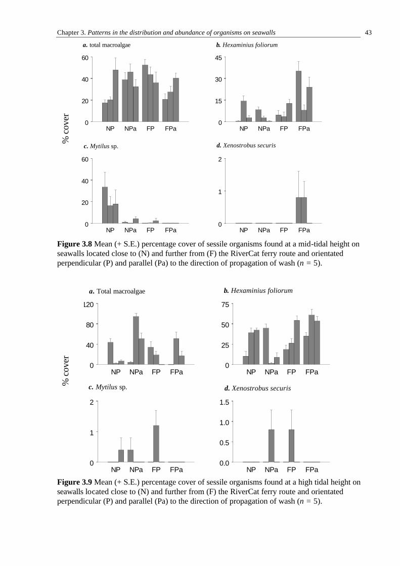
Chapter 3. Patterns in the distribution and abundance of organisms on seawalls
43
Figure 3.8 Mean (+ S.E.) percentage cover of sessile organisms found at a mid-tidal height on seawalls located close to (N) and further from (F) the RiverCat ferry route and orientated perpendicular (P) and parallel (Pa) to the direction of propagation of wash (n = 5).
Figure 3.9 Mean (+ S.E.) percentage cover of sessile organisms found at a high tidal height on seawalls located close to (N) and further from (F) the RiverCat ferry route and orientated perpendicular (P) and parallel (Pa) to the direction of propagation of wash (n = 5).
NP NPa FP FPa0
20
40
60
a. total macroalgae
NP NPa FP FPa0
15
30
45
b. Hexaminius foliorum
NP NPa FP FPa0
20
40
60
c. Mytilus sp.
NP NPa FP FPa0
1
2
d. Xenostrobus securis
% c
over
% c
over
NP NPa FP FPa0
40
80
120
a. Total macroalgae
NP NPa FP FPa0
25
50
75
b. Hexaminius foliorum
NP NPa FP FPa0
1
2
c. Mytilus sp.
NP NPa FP FPa0.0
0.5
1.0
1.5
d. Xenostrobus securis
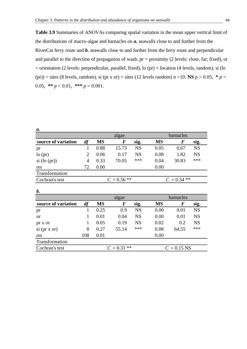
Chapter 3. Patterns in the distribution and abundance of organisms on seawalls
44
Table 3.9 Summaries of ANOVAs comparing spatial variation in the mean upper vertical limit of
the distributions of macro-algae and barnacles on a. seawalls close to and further from the
RiverCat ferry route and b. seawalls close to and further from the ferry route and perpendicular
and parallel to the direction of propagation of wash. pr = proximity (2 levels: close, far; fixed), or
= orientation (2 levels: perpendicular, parallel; fixed), lo (pr) = location (4 levels, random), si (lo
(pr)) = sites (8 levels, random), si (pr x or) = sites (12 levels random) n =10. NS p > 0.05, * p <
0.05, ** p < 0.01, *** p < 0.001.
a.
df MS F sig. MS F sig.pr 1 0.88 15.73 NS 0.05 0.67 NSlo (pr) 2 0.06 0.17 NS 0.08 1.82 NSsi (lo (pr)) 4 0.33 70.05 *** 0.04 30.83 ***res 72 0.00 0.00TransformationCochran's test
b.
df MS F sig. MS F sig.pr 1 0.25 0.9 NS 0.00 0.01 NSor 1 0.01 0.04 NS 0.00 0.01 NSpr x or 1 0.05 0.19 NS 0.02 0.2 NSsi (pr x or) 8 0.27 55.14 *** 0.08 64.55 ***res 108 0.01 0.00TransformationCochran's test C = 0.31 ** C = 0.15 NS
algae barnacles
C = 0.56 ** C = 0.34 **
source of variation
source of variationalgae barnacles
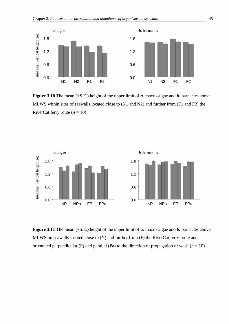
Chapter 3. Patterns in the distribution and abundance of organisms on seawalls
45
Figure 3.10 The mean (+S.E.) height of the upper limit of a. macro-algae and b. barnacles above
MLWS within sites of seawalls located close to (N1 and N2) and further from (F1 and F2) the
RiverCat ferry route (n = 10).
Figure 3.11 The mean (+S.E.) height of the upper limit of a. macro-algae and b. barnacles above
MLWS on seawalls located close to (N) and further from (F) the RiverCat ferry route and
orientated perpendicular (P) and parallel (Pa) to the direction of propagation of wash (n = 10).
NP NPa FP FPa0.0
0.6
1.2
1.8
a. algae
NP NPa FP FPa0.0
0.6
1.2
1.8
b. barnacles
N1 N2 F1 F20.0
0.6
1.2
1.8
a. algae
N1 N2 F1 F20.0
0.6
1.2
1.8
b. barnacles
max
imal
ver
tical
hei
ght (
m)
max
imal
ver
tical
hei
ght (
m)
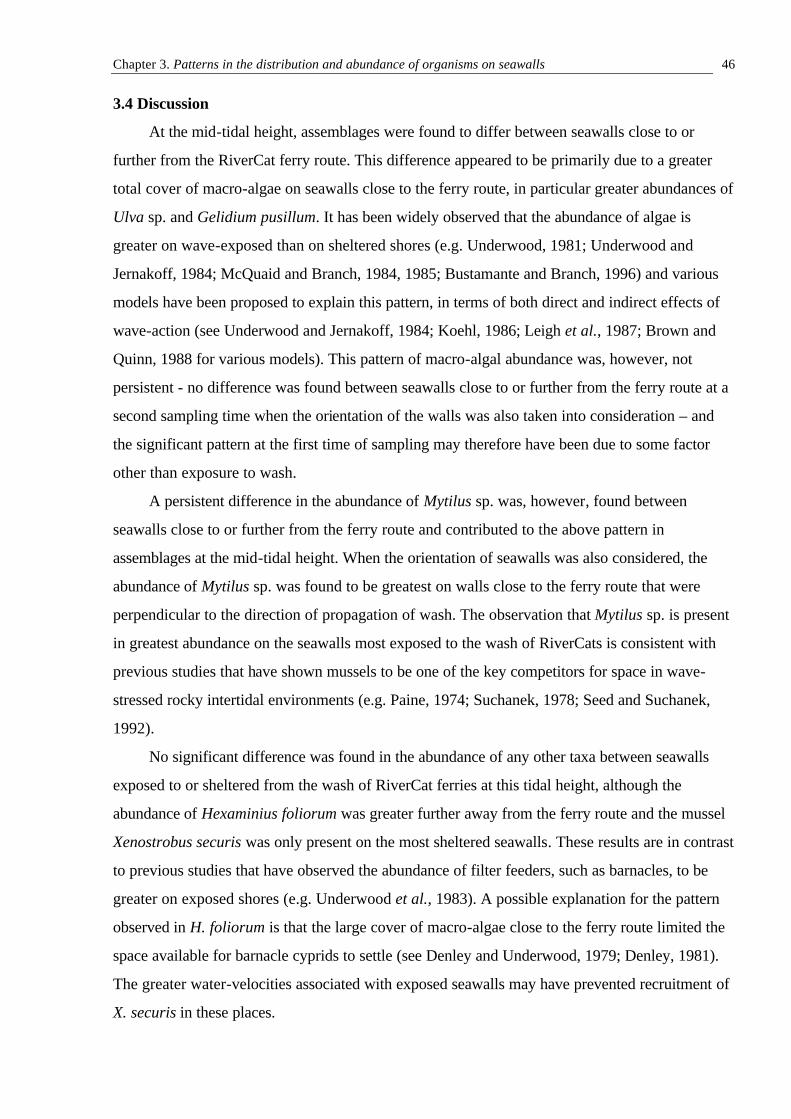
Chapter 3. Patterns in the distribution and abundance of organisms on seawalls
46
3.4 Discussion
At the mid-tidal height, assemblages were found to differ between seawalls close to or
further from the RiverCat ferry route. This difference appeared to be primarily due to a greater
total cover of macro-algae on seawalls close to the ferry route, in particular greater abundances of
Ulva sp. and Gelidium pusillum. It has been widely observed that the abundance of algae is
greater on wave-exposed than on sheltered shores (e.g. Underwood, 1981; Underwood and
Jernakoff, 1984; McQuaid and Branch, 1984, 1985; Bustamante and Branch, 1996) and various
models have been proposed to explain this pattern, in terms of both direct and indirect effects of
wave-action (see Underwood and Jernakoff, 1984; Koehl, 1986; Leigh et al., 1987; Brown and
Quinn, 1988 for various models). This pattern of macro-algal abundance was, however, not
persistent - no difference was found between seawalls close to or further from the ferry route at a
second sampling time when the orientation of the walls was also taken into consideration – and
the significant pattern at the first time of sampling may therefore have been due to some factor
other than exposure to wash.
A persistent difference in the abundance of Mytilus sp. was, however, found between
seawalls close to or further from the ferry route and contributed to the above pattern in
assemblages at the mid-tidal height. When the orientation of seawalls was also considered, the
abundance of Mytilus sp. was found to be greatest on walls close to the ferry route that were
perpendicular to the direction of propagation of wash. The observation that Mytilus sp. is present
in greatest abundance on the seawalls most exposed to the wash of RiverCats is consistent with
previous studies that have shown mussels to be one of the key competitors for space in wave-
stressed rocky intertidal environments (e.g. Paine, 1974; Suchanek, 1978; Seed and Suchanek,
1992).
No significant difference was found in the abundance of any other taxa between seawalls
exposed to or sheltered from the wash of RiverCat ferries at this tidal height, although the
abundance of Hexaminius foliorum was greater further away from the ferry route and the mussel
Xenostrobus securis was only present on the most sheltered seawalls. These results are in contrast
to previous studies that have observed the abundance of filter feeders, such as barnacles, to be
greater on exposed shores (e.g. Underwood et al., 1983). A possible explanation for the pattern
observed in H. foliorum is that the large cover of macro-algae close to the ferry route limited the
space available for barnacle cyprids to settle (see Denley and Underwood, 1979; Denley, 1981).
The greater water-velocities associated with exposed seawalls may have prevented recruitment of
X. securis in these places.
Chapter 3. Patterns in the distribution and abundance of organisms on seawalls
47
At the higher level, no significant difference was found between assemblages or the
abundances of individual species close to or further from the RiverCat route. Moreover, no
difference was found in the mean height of the upper limit at which barnacles or algae were found
between these two treatments, nor between seawalls orientated perpendicular or parallel to
incoming wash, despite the widely-documented observation that the upper boundaries in the
distribution of intertidal organisms are higher in areas exposed to wave-action than in areas that
are sheltered (e.g. Underwood and Jernakoff, 1984).
A number of models may explain the lack of pattern found at the higher level. First,
exposure to waves may be unimportant in determining the ecology of organisms found at a high
level on seawalls. Second, exposure to waves may be important, but the effects might not have
been sufficient for a significant difference to be seen. Third, exposure to waves may be important
in determining the ecology at this height, but wash from RiverCats is unimportant because splash
and spray from other vessels and wind-driven waves wet seawalls to a greater height than does
wash from RiverCats. During this study, it was observed that on very windy days, wind-driven
ways hitting all seawalls were much greater in height than the wash produced by the RiverCat
ferries. Such “extreme” events may be more important in structuring assemblages than regular
events, as suggested by Gaines and Denny (1993).
Significant variability was observed among seawalls close to or further from the ferry route
and perpendicular or parallel to the direction of propagation of wash at the two times of sampling.
The consistency of this variability across treatments suggests that it is due to smaller-scale
processes and is not related to the disturbance caused by RiverCat ferries. Seawalls along the
Parramatta River differ in their small-scale topographic heterogeneity (e.g. the number and size of
cracks and crevices between sandstone blocks and the degree to which the surfaces of blocks have
been abraded) and the depth and topography of the adjacent river-bed. Small-scale topographic
heterogeneity of substrata has been shown to be important in determining the abundance of
individual species and the diversity of assemblages (e.g. Emson and Faller-Fritsch, 1976; Harlin
and Lindburgh, 1977; Woodin, 1978; Menge et al., 1983; Watanuki and Yamomoto, 1990). For
example, many species of algae are more abundant on substrata with coarser particles (Harlin and
Lindburgh, 1977; Watanuki and Yamomoto, 1990), perhaps because such substrata have a
greater area on which to settle, and the abundance of the Littorinid Littorina rudis appears to be
positively affected by the availability of crevices (Emson and Faller-Fritsch, 1976).
Chapter 3. Patterns in the distribution and abundance of organisms on seawalls
48
Differences in the ages of the seawalls may contribute to spatial variability because seawalls
of different ages will have had different histories of disturbance, which can be important in
determining the structure of intertidal assemblages (see Underwood, 1989).
The apparent unimportance of wash from RiverCat ferries in determining the structure of
intertidal assemblages is in contrast to the findings of Blockley (1999). His study, in Sydney
Harbour, found assemblages to differ between seawalls exposed to or sheltered from oceanic
swell, boat-wash and wind-waves. He also found spatial variability to be greater among wave-
exposed seawalls than among sheltered seawalls. The apparent difference in effect of RiverCat-
wash and other waves on the assemblages of seawalls may be a function of the frequency of
waves. In contrast to oceanic swell that constantly hits a shore, the waves resulting from passing
RiverCat ferries are relatively infrequent, occurring around once every fifteen minutes during
daylight hours only. Alternatively, the height of wash from RiverCat ferries may not be great
enough to extend the vertical height to which seawalls are wetted.
At no stage of this study was the energy or height of waves produced by RiverCats
quantified at seawalls close to or further from the ferry route or at seawalls orientated
perpendicular and parallel to incoming wash. It is possible that there was, in fact, no significant
difference in these variables between treatments and that if the assemblages of seawalls that are
completely sheltered from wash were compared with those exposed to wash a difference would
be seen.
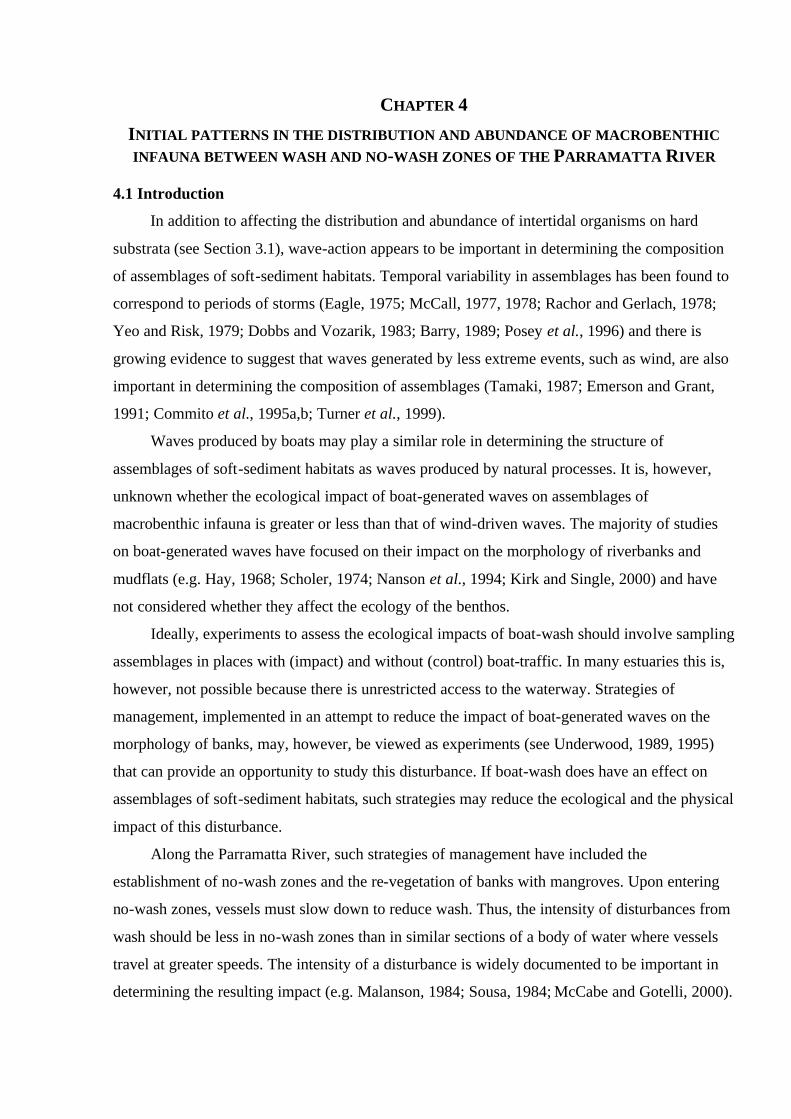
CHAPTER 4
INITIAL PATTERNS IN THE DISTRIBUTION AND ABUNDANCE OF MACROBENTHIC INFAUNA BETWEEN WASH AND NO-WASH ZONES OF THE PARRAMATTA RIVER
4.1 Introduction
In addition to affecting the distribution and abundance of intertidal organisms on hard
substrata (see Section 3.1), wave-action appears to be important in determining the composition
of assemblages of soft-sediment habitats. Temporal variability in assemblages has been found to
correspond to periods of storms (Eagle, 1975; McCall, 1977, 1978; Rachor and Gerlach, 1978;
Yeo and Risk, 1979; Dobbs and Vozarik, 1983; Barry, 1989; Posey et al., 1996) and there is
growing evidence to suggest that waves generated by less extreme events, such as wind, are also
important in determining the composition of assemblages (Tamaki, 1987; Emerson and Grant,
1991; Commito et al., 1995a,b; Turner et al., 1999).
Waves produced by boats may play a similar role in determining the structure of
assemblages of soft-sediment habitats as waves produced by natural processes. It is, however,
unknown whether the ecological impact of boat-generated waves on assemblages of
macrobenthic infauna is greater or less than that of wind-driven waves. The majority of studies
on boat-generated waves have focused on their impact on the morphology of riverbanks and
mudflats (e.g. Hay, 1968; Scholer, 1974; Nanson et al., 1994; Kirk and Single, 2000) and have
not considered whether they affect the ecology of the benthos.
Ideally, experiments to assess the ecological impacts of boat-wash should involve sampling
assemblages in places with (impact) and without (control) boat-traffic. In many estuaries this is,
however, not possible because there is unrestricted access to the waterway. Strategies of
management, implemented in an attempt to reduce the impact of boat-generated waves on the
morphology of banks, may, however, be viewed as experiments (see Underwood, 1989, 1995)
that can provide an opportunity to study this disturbance. If boat-wash does have an effect on
assemblages of soft-sediment habitats, such strategies may reduce the ecological and the physical
impact of this disturbance.
Along the Parramatta River, such strategies of management have included the
establishment of no-wash zones and the re-vegetation of banks with mangroves. Upon entering
no-wash zones, vessels must slow down to reduce wash. Thus, the intensity of disturbances from
wash should be less in no-wash zones than in similar sections of a body of water where vessels
travel at greater speeds. The intensity of a disturbance is widely documented to be important in
determining the resulting impact (e.g. Malanson, 1984; Sousa, 1984; McCabe and Gotelli, 2000).
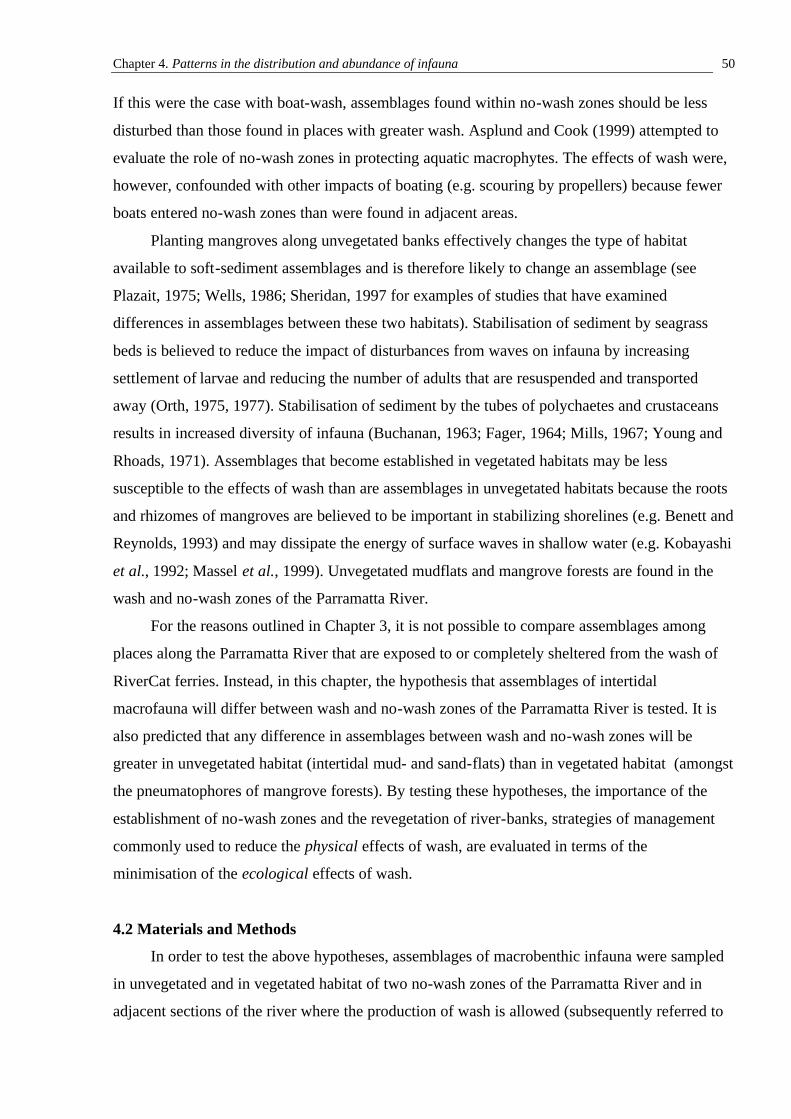
Chapter 4. Patterns in the distribution and abundance of infauna 50
If this were the case with boat-wash, assemblages found within no-wash zones should be less
disturbed than those found in places with greater wash. Asplund and Cook (1999) attempted to
evaluate the role of no-wash zones in protecting aquatic macrophytes. The effects of wash were,
however, confounded with other impacts of boating (e.g. scouring by propellers) because fewer
boats entered no-wash zones than were found in adjacent areas.
Planting mangroves along unvegetated banks effectively changes the type of habitat
available to soft-sediment assemblages and is therefore likely to change an assemblage (see
Plazait, 1975; Wells, 1986; Sheridan, 1997 for examples of studies that have examined
differences in assemblages between these two habitats). Stabilisation of sediment by seagrass
beds is believed to reduce the impact of disturbances from waves on infauna by increasing
settlement of larvae and reducing the number of adults that are resuspended and transported
away (Orth, 1975, 1977). Stabilisation of sediment by the tubes of polychaetes and crustaceans
results in increased diversity of infauna (Buchanan, 1963; Fager, 1964; Mills, 1967; Young and
Rhoads, 1971). Assemblages that become established in vegetated habitats may be less
susceptible to the effects of wash than are assemblages in unvegetated habitats because the roots
and rhizomes of mangroves are believed to be important in stabilizing shorelines (e.g. Benett and
Reynolds, 1993) and may dissipate the energy of surface waves in shallow water (e.g. Kobayashi
et al., 1992; Massel et al., 1999). Unvegetated mudflats and mangrove forests are found in the
wash and no-wash zones of the Parramatta River.
For the reasons outlined in Chapter 3, it is not possible to compare assemblages among
places along the Parramatta River that are exposed to or completely sheltered from the wash of
RiverCat ferries. Instead, in this chapter, the hypothesis that assemblages of intertidal
macrofauna will differ between wash and no-wash zones of the Parramatta River is tested. It is
also predicted that any difference in assemblages between wash and no-wash zones will be
greater in unvegetated habitat (intertidal mud- and sand-flats) than in vegetated habitat (amongst
the pneumatophores of mangrove forests). By testing these hypotheses, the importance of the
establishment of no-wash zones and the revegetation of river-banks, strategies of management
commonly used to reduce the physical effects of wash, are evaluated in terms of the
minimisation of the ecological effects of wash.
4.2 Materials and Methods
In order to test the above hypotheses, assemblages of macrobenthic infauna were sampled
in unvegetated and in vegetated habitat of two no-wash zones of the Parramatta River and in
adjacent sections of the river where the production of wash is allowed (subsequently referred to
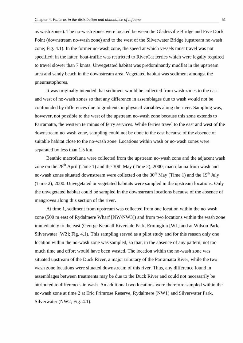
Chapter 4. Patterns in the distribution and abundance of infauna 51
as wash zones). The no-wash zones were located between the Gladesville Bridge and Five Dock
Point (downstream no-wash zone) and to the west of the Silverwater Bridge (upstream no-wash
zone; Fig. 4.1). In the former no-wash zone, the speed at which vessels must travel was not
specified; in the latter, boat-traffic was restricted to RiverCat ferries which were legally required
to travel slower than 7 knots. Unvegetated habitat was predominantly mudflat in the upstream
area and sandy beach in the downstream area. Vegetated habitat was sediment amongst the
pneumatophores.
It was originally intended that sediment would be collected from wash zones to the east
and west of no-wash zones so that any difference in assemblages due to wash would not be
confounded by differences due to gradients in physical variables along the river. Sampling was,
however, not possible to the west of the upstream no-wash zone because this zone extends to
Parramatta, the western terminus of ferry services. While ferries travel to the east and west of the
downstream no-wash zone, sampling could not be done to the east because of the absence of
suitable habitat close to the no-wash zone. Locations within wash or no-wash zones were
separated by less than 1.5 km.
Benthic macrofauna were collected from the upstream no-wash zone and the adjacent wash
zone on the 28th April (Time 1) and the 30th May (Time 2), 2000; macrofauna from wash and
no-wash zones situated downstream were collected on the 30th May (Time 1) and the 19th July
(Time 2), 2000. Unvegetated or vegetated habitats were sampled in the upstream locations. Only
the unvegetated habitat could be sampled in the downstream locations because of the absence of
mangroves along this section of the river.
At time 1, sediment from upstream was collected from one location within the no-wash
zone (500 m east of Rydalmere Wharf [NW/NW3]) and from two locations within the wash zone
immediately to the east (George Kendall Riverside Park, Ermington [W1] and at Wilson Park,
Silverwater [W2]; Fig. 4.1). This sampling served as a pilot study and for this reason only one
location within the no-wash zone was sampled, so that, in the absence of any pattern, not too
much time and effort would have been wasted. The location within the no-wash zone was
situated upstream of the Duck River, a major tributary of the Parramatta River, while the two
wash zone locations were situated downstream of this river. Thus, any difference found in
assemblages between treatments may be due to the Duck River and could not necessarily be
attributed to differences in wash. An additional two locations were therefore sampled within the
no-wash zone at time 2 at Eric Primrose Reserve, Rydalmere (NW1) and Silverwater Park,
Silverwater (NW2; Fig. 4.1).
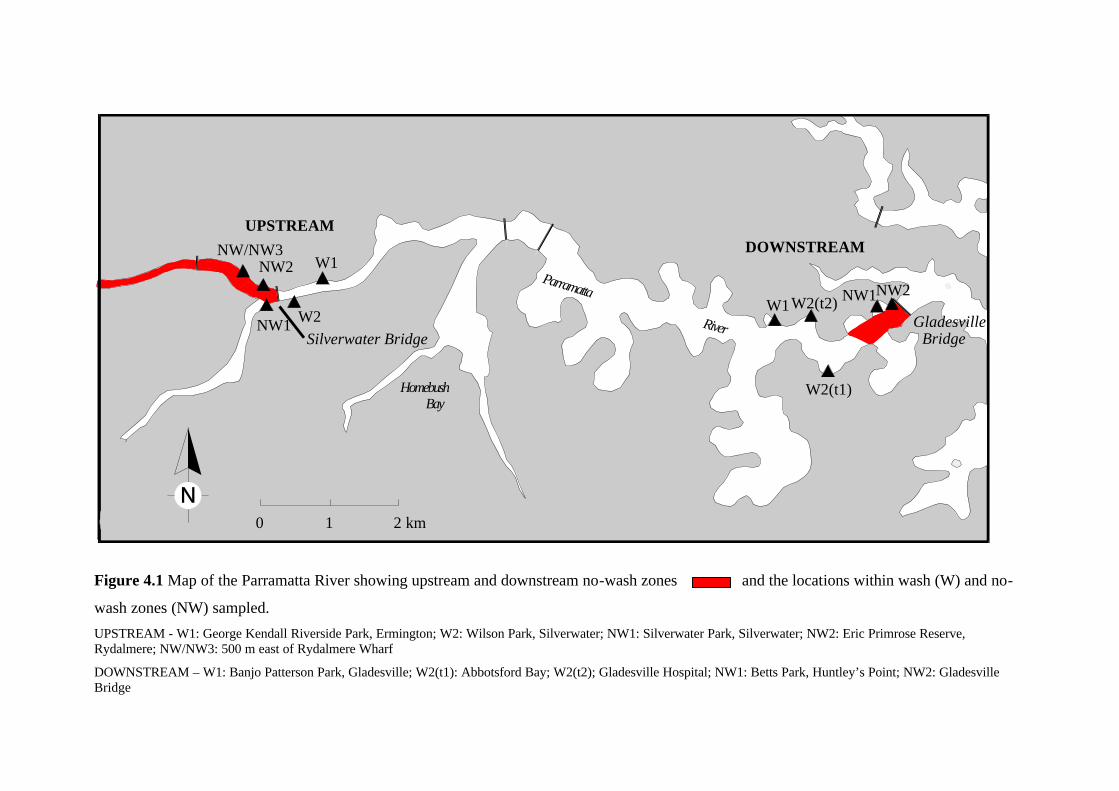
Figure 4.1 Map of the Parramatta River showing upstream and downstream no-wash zones and the locations within wash (W) and no-
wash zones (NW) sampled.
UPSTREAM - W1: George Kendall Riverside Park, Ermington; W2: Wilson Park, Silverwater; NW1: Silverwater Park, Silverwater; NW2: Eric Primrose Reserve, Rydalmere; NW/NW3: 500 m east of Rydalmere Wharf
DOWNSTREAM – W1: Banjo Patterson Park, Gladesville; W2(t1): Abbotsford Bay; W2(t2); Gladesville Hospital; NW1: Betts Park, Huntley’s Point; NW2: Gladesville Bridge
Parramatta
River
HomebushBay
W1
W2
NW2NW/NW3
NW1W1
W2(t1)
NW1NW2W2(t2)
0 2 km1
UPSTREAMDOWNSTREAM
Silverwater BridgeGladesville
Bridge
Chapter 4. Patterns in the distribution and abundance of infauna 53
Within the downstream no-wash zone, sediment was collected from Betts Park, Huntley’s
Point (NW1) and 100 m west of the Gladesville Bridge (NW2) at times 1 and 2. Sediment was
collected from the wash zone to the east at Banjo Patterson Park, Gladesville (W1) and
Abbotsford Bay (W2(t1)) at Time 1. At time 2, sediment was collected from Gladesville
Hospital (W2(t2)) instead of Abbotsford Bay so that all locations, within wash or no-wash zones,
would be situated on the northern bank of the river (Fig. 4.1). In the no-wash zone, it was not
possible to sample on the southern side of the river because of the absence of suitable habitat.
Within each location, two sites, approximately 15 m long were randomly selected, 10s of
metres apart. In the upstream locations, these sites contained unvegetated and vegetated habitats
which were, wherever possible, at roughly the same tidal height and distance from the centre of
the river. Five cores of sediment were haphazardly collected from each of the types of habitat
within each site and transported back to the laboratory for processing and sorting (see Section
2.5.2 for a full description of the sampling method).
Differences between the assemblages in wash and no-wash zones were examined using
nMDS ordinations of centroids representing sites and NP-MANOVAs (Anderson, 2001) and
ANOSIMs (Clarke, 1993) of untransformed data. NP-MANOVAs and ANOSIMs were done
because NP-MANOVAs test hypotheses regarding multivariate distances (measures of
dissimilarity) whereas ANOSIMs test hypotheses regarding rank-dissimilarities. Presence-
absence data were also analysed to test the hypothesis that differences in assemblages would be
primarily due to differences in the types of organisms present and their distribution among
samples.
Only two factors can be included in ANOSIMs and NP-MANOVAs. The factor,
location, was omitted from ANOSIMs testing for differences between zones within each of the
habitats because nMDS plots indicated great variability at the scale of sites. NP-MANOVAs for
data collected from the upper Parramatta River at time 2 and the lower Parramatta River at each
of the times also included the factors, zone and site. In the case of the data collected from the
upper Parramatta River at time 1, the two factors analysed were locations and sites because
different numbers of sites were sampled in each of the zones and NP-MANOVAs cannot handle
unbalanced sampling designs. The hypothesised interaction between zone and habitat was tested
for using NP-MANOVAs with the factors habitat and site.
Increased variability among samples has been hypothesized to be a general feature of
stressed environments (Warwick and Clarke, 1993; but see Chapman et al., 1995 for an example
where this is not the case). Therefore, Bray-Curtis measures of within-site variability, calculated
in the above analyses, were compared among sites of the upper Parramatta River to test the
Chapter 4. Patterns in the distribution and abundance of infauna 54
hypotheses that, within each of the habitats, variability among: (i) cores and (ii) sites would be
greater in the wash than in the no-wash zone.
ANOVAs were done to test the hypothesis that abundances of individual taxa would be
smaller in the wash zone than the no-wash zone. Because assemblages were fairly depauperate,
ANOVAs were done using the taxa present in a majority of sites in either the wash or no-wash
zone. Two-tailed F-tests of variances, (i) among cores in the wash zone versus among cores in
the no-wash zone and (ii) among sites in the wash zone versus among sites in the no-wash zone,
were done to test the hypothesis that spatial variability at each of these scales would be greater in
the wash than in the no-wash zones.
4.3 Results
Assemblages of the upper Parramatta River were dominated by polychaetes of the
families Capitellidae and Nereididae (Table 4.1). Assemblages further downstream were
dominated by syllids.
4.3.1 Upper Parramatta River
At each time of sampling, untransformed data appeared to separate into two groups
corresponding to wash and no-wash zones (Fig. 4.2). At time 1, this separation of points
appeared to be greater within the unvegetated habitat than the vegetated habitat. No such
difference was, however, evident at time 2. On the plots of presence-absence data, some
separation of points into groups corresponding to wash and no-wash zones was evident for each
habitat, although patterns were less clear than on plots of untransformed data. At time 2, the taxa
present in the unvegetated habitat of W1(S2) differed from those in all other sites. This pattern
appeared to be driven by the absence of Nereididae from W1(S2). The persistent difference in
the assemblages of wash and no-wash zones across both times of sampling indicates that the
sampling done at time 1 was not confounded by the situation of sites relative to the Duck River.
At time 1, only 15 permutations of data were possible for ANOSIM tests for differences
between the zones because of the small number of sites sampled in the wash or no-wash zone.
Thus, tests could only be significant if all of the permutations produced a test statistic less than
R. It was not surprising, then, that all of the tests for differences between zones at time 1 were
non-significant (Table 4.2a). The large (0.93) sample statistic, R, calculated for the
untransformed data from the unvegetated sediment does, however, indicate that assemblages
differed between wash and no-wash zones (Table 4.2a(i)), as indicated by the nMDS (Fig.
4.2a(i)). At time 2, more permutations were possible due to the larger number of sites sampled.
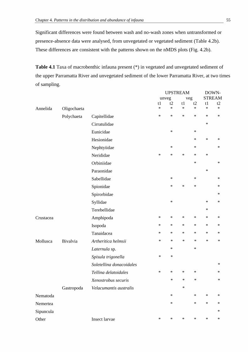
Chapter 4. Patterns in the distribution and abundance of infauna 55
Significant differences were found between wash and no-wash zones when untransformed or
presence-absence data were analysed, from unvegetated or vegetated sediment (Table 4.2b).
These differences are consistent with the patterns shown on the nMDS plots (Fig. 4.2b).
Table 4.1 Taxa of macrobenthic infauna present (*) in vegetated and unvegetated sediment of
the upper Parramatta River and unvegetated sediment of the lower Parramatta River, at two times
of sampling.
UPSTREAM DOWN- unveg veg STREAM t1 t2 t1 t2 t1 t2 Annelida Oligochaeta * * * * * *
Polychaeta Capitellidae * * * * * *
Cirratulidae *
Eunicidae * *
Hesionidae * * *
Nephtyiidae * * *
Nerididae * * * * *
Orbiniidae * *
Paraonidae *
Sabellidae * * *
Spionidae * * * *
Spirorbidae *
Syllidae * * *
Terebellidae *
Crustacea Amphipoda * * * * * *
Isopoda * * * * * *
Tanaidacea * * * * * *
Mollusca Bivalvia Artheritica helmsii * * * * * *
Laternula sp. * *
Spisula trigonella * *
Soletellina donacoidales *
Tellina delatoidales * * * * *
Xenostrobus securis * * * *
Gastropoda Velacumantis australis *
Nematoda * * * *
Nemertea * * * *
Sipuncula *
Other Insect larvae * * * * * *
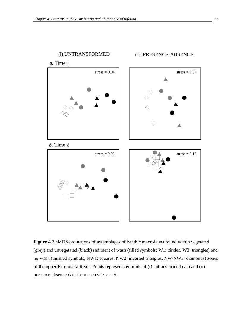
Chapter 4. Patterns in the distribution and abundance of infauna 56
stress = 0.04 stress = 0.07
stress = 0.06 stress = 0.13
a. Time 1
b. Time 2
(i) UNTRANSFORMED (ii) PRESENCE-ABSENCE
Figure 4.2 nMDS ordinations of assemblages of benthic macrofauna found within vegetated
(grey) and unvegetated (black) sediment of wash (filled symbols; W1: circles, W2: triangles) and
no-wash (unfilled symbols; NW1: squares, NW2: inverted triangles, NW/NW3: diamonds) zones
of the upper Parramatta River. Points represent centroids of (i) untransformed data and (ii)
presence-absence data from each site. n = 5.
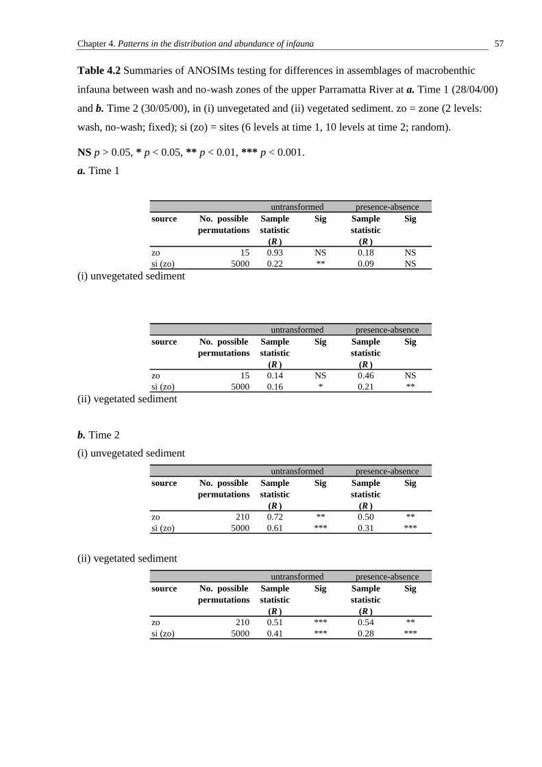
Chapter 4. Patterns in the distribution and abundance of infauna 57
Table 4.2 Summaries of ANOSIMs testing for differences in assemblages of macrobenthic
infauna between wash and no-wash zones of the upper Parramatta River at a. Time 1 (28/04/00)
and b. Time 2 (30/05/00), in (i) unvegetated and (ii) vegetated sediment. zo = zone (2 levels:
wash, no-wash; fixed); si (zo) = sites (6 levels at time 1, 10 levels at time 2; random).
NS p > 0.05, * p < 0.05, ** p < 0.01, *** p < 0.001.
a. Time 1
(i) unvegetated sediment
(ii) vegetated sediment
b. Time 2
(i) unvegetated sediment
(ii) vegetated sediment
source No. possible permutations
Sample statistic
(R )
Sig Sample statistic
(R )
Sig
zo 15 0.93 NS 0.18 NSsi (zo) 5000 0.22 ** 0.09 NS
untransformed presence-absence
source No. possible permutations
Sample statistic
(R )
Sig Sample statistic
(R )
Sig
zo 15 0.14 NS 0.46 NSsi (zo) 5000 0.16 * 0.21 **
untransformed presence-absence
source No. possible permutations
Sample statistic
(R )
Sig Sample statistic
(R )
Sig
zo 210 0.72 ** 0.50 **si (zo) 5000 0.61 *** 0.31 ***
untransformed presence-absence
source No. possible permutations
Sample statistic
(R )
Sig Sample statistic
(R )
Sig
zo 210 0.51 *** 0.54 **si (zo) 5000 0.41 *** 0.28 ***
untransformed presence-absence
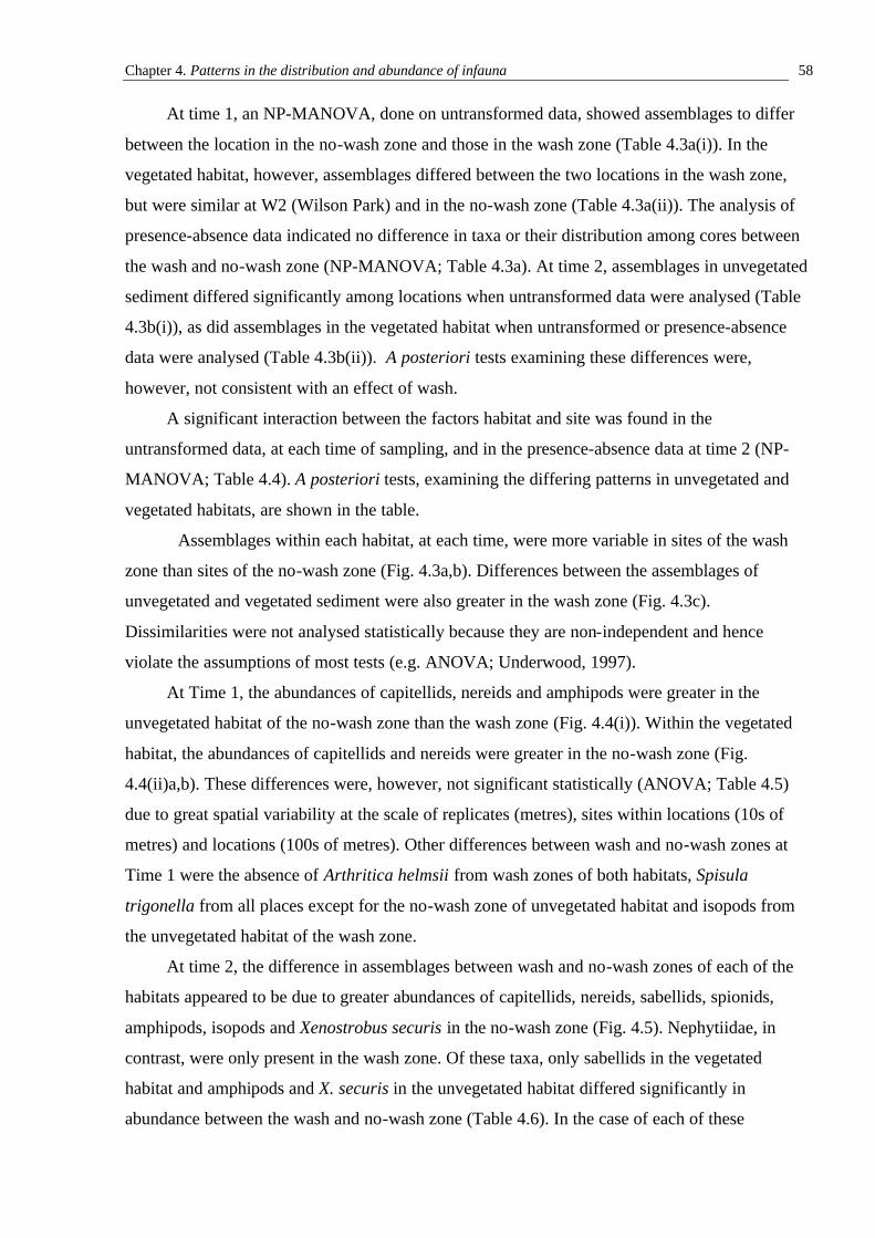
Chapter 4. Patterns in the distribution and abundance of infauna 58
At time 1, an NP-MANOVA, done on untransformed data, showed assemblages to differ
between the location in the no-wash zone and those in the wash zone (Table 4.3a(i)). In the
vegetated habitat, however, assemblages differed between the two locations in the wash zone,
but were similar at W2 (Wilson Park) and in the no-wash zone (Table 4.3a(ii)). The analysis of
presence-absence data indicated no difference in taxa or their distribution among cores between
the wash and no-wash zone (NP-MANOVA; Table 4.3a). At time 2, assemblages in unvegetated
sediment differed significantly among locations when untransformed data were analysed (Table
4.3b(i)), as did assemblages in the vegetated habitat when untransformed or presence-absence
data were analysed (Table 4.3b(ii)). A posteriori tests examining these differences were,
however, not consistent with an effect of wash.
A significant interaction between the factors habitat and site was found in the
untransformed data, at each time of sampling, and in the presence-absence data at time 2 (NP-
MANOVA; Table 4.4). A posteriori tests, examining the differing patterns in unvegetated and
vegetated habitats, are shown in the table.
Assemblages within each habitat, at each time, were more variable in sites of the wash
zone than sites of the no-wash zone (Fig. 4.3a,b). Differences between the assemblages of
unvegetated and vegetated sediment were also greater in the wash zone (Fig. 4.3c).
Dissimilarities were not analysed statistically because they are non-independent and hence
violate the assumptions of most tests (e.g. ANOVA; Underwood, 1997).
At Time 1, the abundances of capitellids, nereids and amphipods were greater in the
unvegetated habitat of the no-wash zone than the wash zone (Fig. 4.4(i)). Within the vegetated
habitat, the abundances of capitellids and nereids were greater in the no-wash zone (Fig.
4.4(ii)a,b). These differences were, however, not significant statistically (ANOVA; Table 4.5)
due to great spatial variability at the scale of replicates (metres), sites within locations (10s of
metres) and locations (100s of metres). Other differences between wash and no-wash zones at
Time 1 were the absence of Arthritica helmsii from wash zones of both habitats, Spisula
trigonella from all places except for the no-wash zone of unvegetated habitat and isopods from
the unvegetated habitat of the wash zone.
At time 2, the difference in assemblages between wash and no-wash zones of each of the
habitats appeared to be due to greater abundances of capitellids, nereids, sabellids, spionids,
amphipods, isopods and Xenostrobus securis in the no-wash zone (Fig. 4.5). Nephytiidae, in
contrast, were only present in the wash zone. Of these taxa, only sabellids in the vegetated
habitat and amphipods and X. securis in the unvegetated habitat differed significantly in
abundance between the wash and no-wash zone (Table 4.6). In the case of each of these
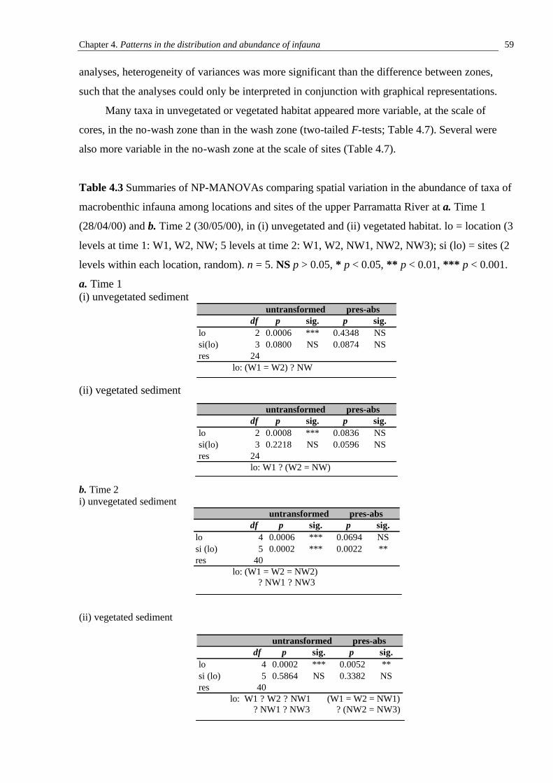
Chapter 4. Patterns in the distribution and abundance of infauna 59
analyses, heterogeneity of variances was more significant than the difference between zones,
such that the analyses could only be interpreted in conjunction with graphical representations.
Many taxa in unvegetated or vegetated habitat appeared more variable, at the scale of
cores, in the no-wash zone than in the wash zone (two-tailed F-tests; Table 4.7). Several were
also more variable in the no-wash zone at the scale of sites (Table 4.7).
Table 4.3 Summaries of NP-MANOVAs comparing spatial variation in the abundance of taxa of
macrobenthic infauna among locations and sites of the upper Parramatta River at a. Time 1
(28/04/00) and b. Time 2 (30/05/00), in (i) unvegetated and (ii) vegetated habitat. lo = location (3
levels at time 1: W1, W2, NW; 5 levels at time 2: W1, W2, NW1, NW2, NW3); si (lo) = sites (2
levels within each location, random). n = 5. NS p > 0.05, * p < 0.05, ** p < 0.01, *** p < 0.001.
a. Time 1 (i) unvegetated sediment
lo: (W1 = W2) ? NW
(ii) vegetated sediment
lo: W1 ? (W2 = NW)
b. Time 2 i) unvegetated sediment
lo: (W1 = W2 = NW2) ? NW1 ? NW3
(ii) vegetated sediment
lo: W1 ? W2 ? NW1 (W1 = W2 = NW1) ? NW1 ? NW3 ? (NW2 = NW3)
df p sig. p sig.lo 2 0.0006 *** 0.4348 NSsi(lo) 3 0.0800 NS 0.0874 NSres 24
untransformed pres-abs
df p sig. p sig.lo 2 0.0008 *** 0.0836 NSsi(lo) 3 0.2218 NS 0.0596 NSres 24
untransformed pres-abs
df p sig. p sig.lo 4 0.0006 *** 0.0694 NSsi (lo) 5 0.0002 *** 0.0022 **res 40
untransformed pres-abs
df p sig. p sig.lo 4 0.0002 *** 0.0052 **si (lo) 5 0.5864 NS 0.3382 NSres 40
untransformed pres-abs
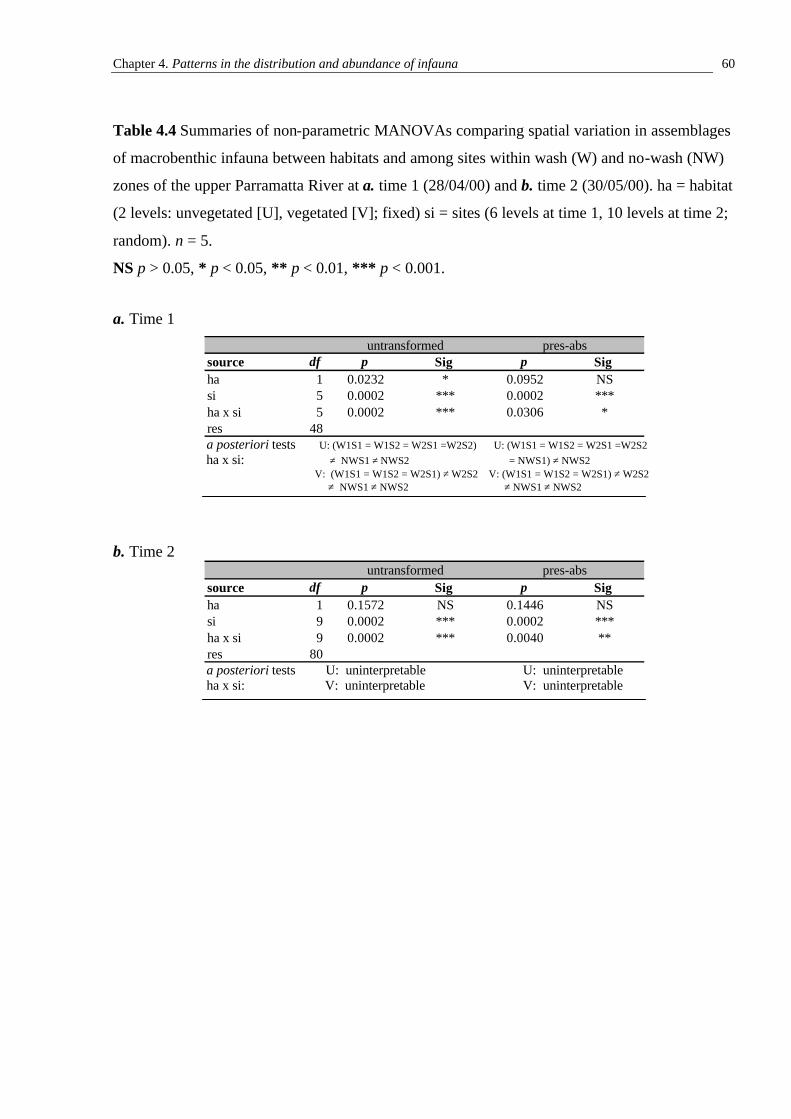
Chapter 4. Patterns in the distribution and abundance of infauna 60
Table 4.4 Summaries of non-parametric MANOVAs comparing spatial variation in assemblages
of macrobenthic infauna between habitats and among sites within wash (W) and no-wash (NW)
zones of the upper Parramatta River at a. time 1 (28/04/00) and b. time 2 (30/05/00). ha = habitat
(2 levels: unvegetated [U], vegetated [V]; fixed) si = sites (6 levels at time 1, 10 levels at time 2;
random). n = 5.
NS p > 0.05, * p < 0.05, ** p < 0.01, *** p < 0.001.
a. Time 1
a posteriori tests U: (W1S1 = W1S2 = W2S1 =W2S2) U: (W1S1 = W1S2 = W2S1 =W2S2 ha x si: ≠ NWS1 ≠ NWS2 = NWS1) ≠ NWS2 V: (W1S1 = W1S2 = W2S1) ≠ W2S2 V: (W1S1 = W1S2 = W2S1) ≠ W2S2 ≠ NWS1 ≠ NWS2 ≠ NWS1 ≠ NWS2
b. Time 2
a posteriori tests U: uninterpretable U: uninterpretable ha x si: V: uninterpretable V: uninterpretable
source df p Sig p Sig ha 1 0.0232 * 0.0952 NSsi 5 0.0002 *** 0.0002 ***ha x si 5 0.0002 *** 0.0306 *res 48
untransformed pres-abs
source df p Sig p Sig ha 1 0.1572 NS 0.1446 NSsi 9 0.0002 *** 0.0002 ***ha x si 9 0.0002 *** 0.0040 **res 80
untransformed pres-abs
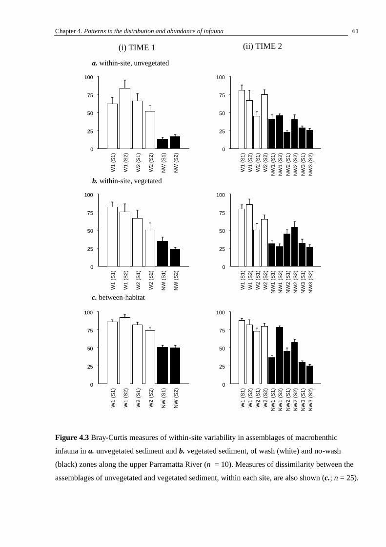
Chapter 4. Patterns in the distribution and abundance of infauna 61
W1
(S1)
W1
(S2)
W2
(S1)
W2
(S2)
NW
(S1)
NW
(S2)
0
25
50
75
100
a. within-site, unvegetated
W1
(S1)
W1
(S2)
W2
(S1)
W2
(S2)
NW
1 (S
1)N
W1
(S2)
NW
2 (S
1)N
W2
(S2)
NW
3 (S
1)N
W3
(S2)
0
25
50
75
100
W1
(S1)
W1
(S2)
W2
(S1)
W2
(S2)
NW
(S
1)
NW
(S
2)
0
25
50
75
100
W1
(S1)
W1
(S2)
W2
(S1)
W2
(S2)
NW
1 (S
1)N
W1
(S2)
NW
2 (S
1)N
W2
(S2)
NW
3 (S
1)N
W3
(S2)
0
25
50
75
100
W1
(S1)
W1
(S2)
W2
(S1)
W2
(S2)
NW
(S
1)
NW
(S
2)
0
25
50
75
100
W1
(S1)
W1
(S2)
W2
(S1)
W2
(S2)
NW
1 (S
1)N
W1
(S2)
NW
2 (S
1)N
W2
(S2)
NW
3 (S
1)N
W3
(S2)
0
25
50
75
100
b. within-site, vegetated
c. between-habitat
(i) TIME 1 (ii) TIME 2
Figure 4.3 Bray-Curtis measures of within-site variability in assemblages of macrobenthic
infauna in a. unvegetated sediment and b. vegetated sediment, of wash (white) and no-wash
(black) zones along the upper Parramatta River (n = 10). Measures of dissimilarity between the
assemblages of unvegetated and vegetated sediment, within each site, are also shown (c.; n = 25).
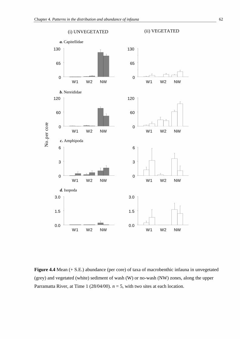
Chapter 4. Patterns in the distribution and abundance of infauna 62
Figure 4.4 Mean (+ S.E.) abundance (per core) of taxa of macrobenthic infauna in unvegetated
(grey) and vegetated (white) sediment of wash (W) or no-wash (NW) zones, along the upper
Parramatta River, at Time 1 (28/04/00). n = 5, with two sites at each location.
W1 W2 NW0
65
130
W1 W2 NW0
65
130
W1 W2 NW0
60
120
W1 W2 NW0
60
120
W1 W2 NW0
3
6
W1 W2 NW0
3
6
W1 W2 NW0.0
1.5
3.0
W1 W2 NW0.0
1.5
3.0
a. Capitellidae
b. Nereididae
c. Amphipoda
d. Isopoda
(i) UNVEGETATED (ii) VEGETATED
No.
per
core
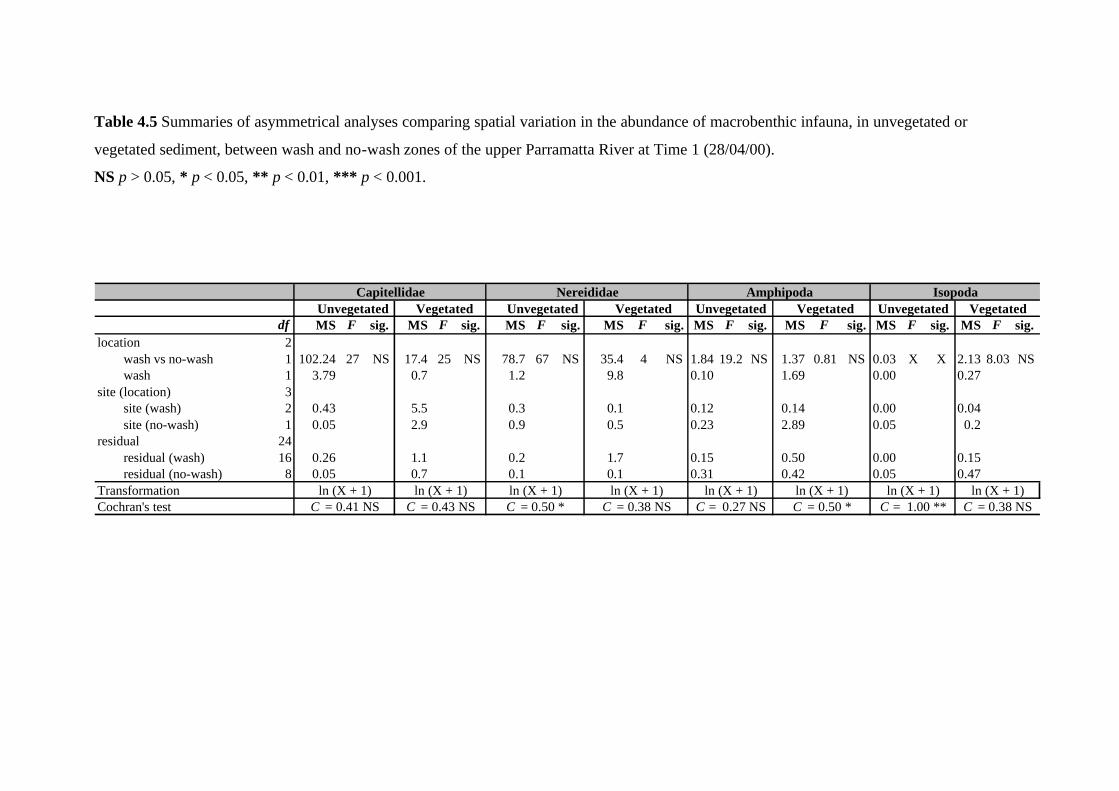
Table 4.5 Summaries of asymmetrical analyses comparing spatial variation in the abundance of macrobenthic infauna, in unvegetated or
vegetated sediment, between wash and no-wash zones of the upper Parramatta River at Time 1 (28/04/00).
NS p > 0.05, * p < 0.05, ** p < 0.01, *** p < 0.001.
Unvegetated Vegetated Unvegetated Vegetated Unvegetated Vegetated Unvegetated Vegetateddf MS F sig. MS F sig. MS F sig. MS F sig. MS F sig. MS F sig. MS F sig. MS F sig.
location 2wash vs no-wash 1 102.24 27 NS 17.4 25 NS 78.7 67 NS 35.4 4 NS 1.84 19.2 NS 1.37 0.81 NS 0.03 X X 2.13 8.03 NSwash 1 3.79 0.7 1.2 9.8 0.10 1.69 0.00 0.27
site (location) 3site (wash) 2 0.43 5.5 0.3 0.1 0.12 0.14 0.00 0.04site (no-wash) 1 0.05 2.9 0.9 0.5 0.23 2.89 0.05 0.2
residual 24residual (wash) 16 0.26 1.1 0.2 1.7 0.15 0.50 0.00 0.15residual (no-wash) 8 0.05 0.7 0.1 0.1 0.31 0.42 0.05 0.47
TransformationCochran's test
ln (X + 1) ln (X + 1)ln (X + 1)C = 0.38 NS
Capitellidae Nereididae
ln (X + 1)C = 0.41 NS C = 0.50 *C = 0.43 NS
ln (X + 1) ln (X + 1)
Amphipoda Isopoda
C = 0.38 NSC = 0.50 * C = 1.00 **C = 0.27 NSln (X + 1) ln (X + 1)
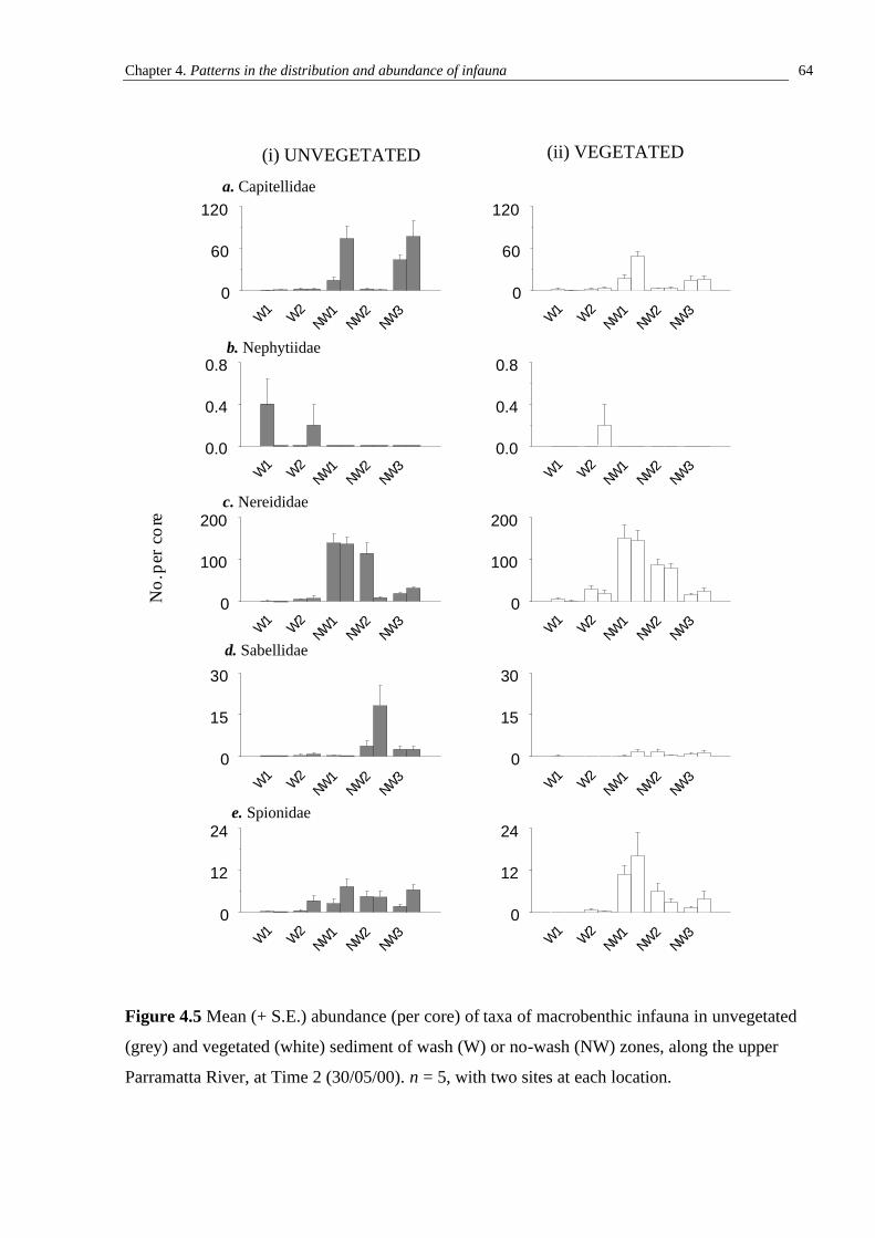
Chapter 4. Patterns in the distribution and abundance of infauna 64
Figure 4.5 Mean (+ S.E.) abundance (per core) of taxa of macrobenthic infauna in unvegetated
(grey) and vegetated (white) sediment of wash (W) or no-wash (NW) zones, along the upper
Parramatta River, at Time 2 (30/05/00). n = 5, with two sites at each location.
No.
per
core
W1 W2NW1
NW2NW3
0
60
120
W1 W2NW1
NW2NW3
0
60
120
W1 W2NW1
NW2NW3
0.0
0.4
0.8
W1 W2NW1
NW2NW3
0.0
0.4
0.8
W1 W2NW1
NW2NW3
0
100
200
W1 W2NW1
NW2NW3
0
100
200
W1 W2NW1
NW2NW3
0
15
30
d. Sabellidae
W1 W2NW1
NW2NW3
0
15
30
W1 W2NW1
NW2NW3
0
12
24e. Spionidae
W1 W2NW1
NW2NW3
0
12
24
a. Capitellidae
b. Nephytiidae
c. Nereididae
(i) UNVEGETATED (ii) VEGETATED
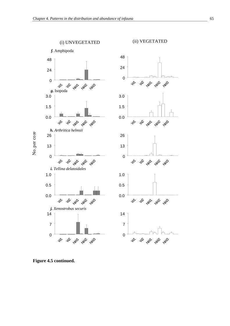
Chapter 4. Patterns in the distribution and abundance of infauna 65
Figure 4.5 continued.
No.
per
core
W1 W2NW1
NW2NW3
0
24
48
W1 W2NW1
NW2NW3
0
24
48
W1 W2NW
1NW
2NW3
0.0
1.5
3.0g. Isopoda
W1 W2NW
1NW2
NW30.0
1.5
3.0
W1 W2NW
1NW
2NW3
0
13
26
W1 W2NW
1NW2
NW30
13
26
W1 W2NW1
NW2NW3
0.0
0.5
1.0
W1 W2NW1
NW2NW3
0.0
0.5
1.0
W1 W2NW
1NW
2NW3
0
7
14
W1 W2NW
1NW2
NW30
7
14
f. Amphipoda
h. Arthritica helmsii
i. Tellina delatoidales
j. Xenostrobus securis
(i) UNVEGETATED (ii) VEGETATED
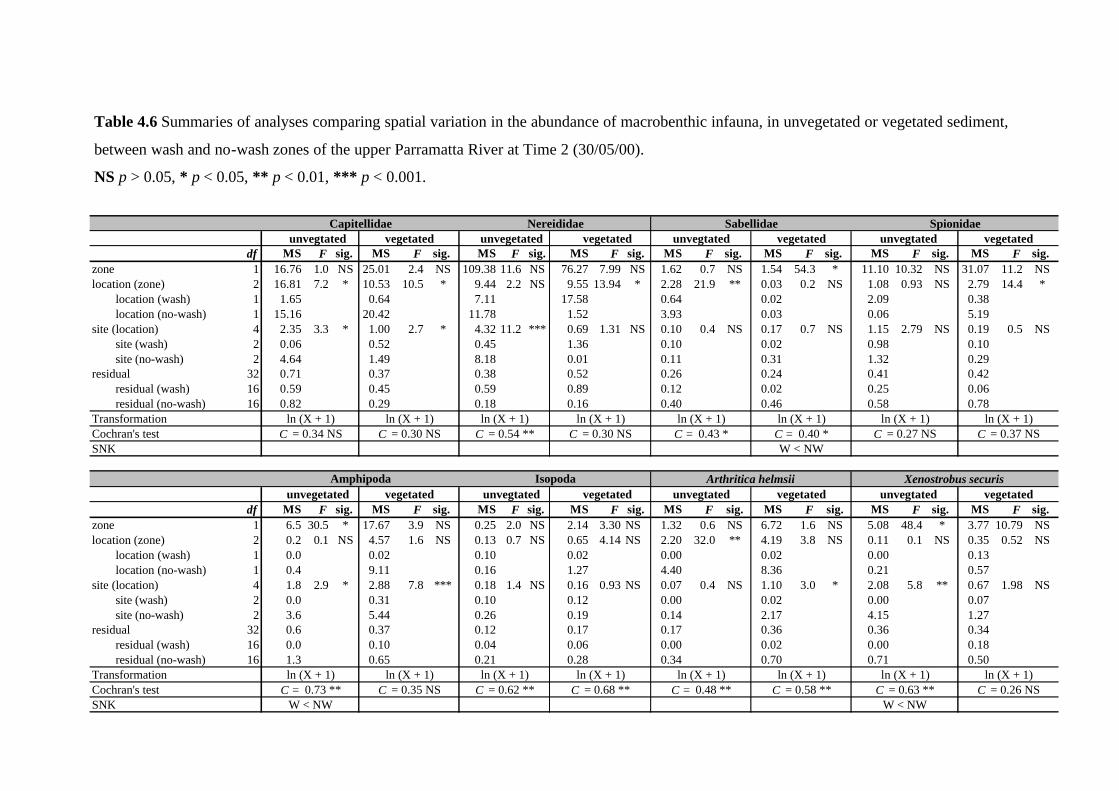
Table 4.6 Summaries of analyses comparing spatial variation in the abundance of macrobenthic infauna, in unvegetated or vegetated sediment,
between wash and no-wash zones of the upper Parramatta River at Time 2 (30/05/00).
NS p > 0.05, * p < 0.05, ** p < 0.01, *** p < 0.001.
unvegtated vegetated unvegetated vegetated unvegtated vegetated unvegtated vegetateddf MS F sig. MS F sig. MS F sig. MS F sig. MS F sig. MS F sig. MS F sig. MS F sig.
zone 1 16.76 1.0 NS 25.01 2.4 NS 109.38 11.6 NS 76.27 7.99 NS 1.62 0.7 NS 1.54 54.3 * 11.10 10.32 NS 31.07 11.2 NSlocation (zone) 2 16.81 7.2 * 10.53 10.5 * 9.44 2.2 NS 9.55 13.94 * 2.28 21.9 ** 0.03 0.2 NS 1.08 0.93 NS 2.79 14.4 *
location (wash) 1 1.65 0.64 7.11 17.58 0.64 0.02 2.09 0.38location (no-wash) 1 15.16 20.42 11.78 1.52 3.93 0.03 0.06 5.19
site (location) 4 2.35 3.3 * 1.00 2.7 * 4.32 11.2 *** 0.69 1.31 NS 0.10 0.4 NS 0.17 0.7 NS 1.15 2.79 NS 0.19 0.5 NSsite (wash) 2 0.06 0.52 0.45 1.36 0.10 0.02 0.98 0.10site (no-wash) 2 4.64 1.49 8.18 0.01 0.11 0.31 1.32 0.29
residual 32 0.71 0.37 0.38 0.52 0.26 0.24 0.41 0.42residual (wash) 16 0.59 0.45 0.59 0.89 0.12 0.02 0.25 0.06residual (no-wash) 16 0.82 0.29 0.18 0.16 0.40 0.46 0.58 0.78
TransformationCochran's testSNK
unvegetated vegetated unvegtated vegetated unvegtated vegetated unvegtated vegetateddf MS F sig. MS F sig. MS F sig. MS F sig. MS F sig. MS F sig. MS F sig. MS F sig.
zone 1 6.5 30.5 * 17.67 3.9 NS 0.25 2.0 NS 2.14 3.30 NS 1.32 0.6 NS 6.72 1.6 NS 5.08 48.4 * 3.77 10.79 NSlocation (zone) 2 0.2 0.1 NS 4.57 1.6 NS 0.13 0.7 NS 0.65 4.14 NS 2.20 32.0 ** 4.19 3.8 NS 0.11 0.1 NS 0.35 0.52 NS
location (wash) 1 0.0 0.02 0.10 0.02 0.00 0.02 0.00 0.13location (no-wash) 1 0.4 9.11 0.16 1.27 4.40 8.36 0.21 0.57
site (location) 4 1.8 2.9 * 2.88 7.8 *** 0.18 1.4 NS 0.16 0.93 NS 0.07 0.4 NS 1.10 3.0 * 2.08 5.8 ** 0.67 1.98 NSsite (wash) 2 0.0 0.31 0.10 0.12 0.00 0.02 0.00 0.07site (no-wash) 2 3.6 5.44 0.26 0.19 0.14 2.17 4.15 1.27
residual 32 0.6 0.37 0.12 0.17 0.17 0.36 0.36 0.34residual (wash) 16 0.0 0.10 0.04 0.06 0.00 0.02 0.00 0.18residual (no-wash) 16 1.3 0.65 0.21 0.28 0.34 0.70 0.71 0.50
TransformationCochran's testSNK W < NW
W < NW
W < NWC = 0.63 ** C = 0.26 NS
ln (X + 1)ln (X + 1)
Spionidae
ln (X + 1) ln (X + 1)C = 0.34 NS C = 0.54 ** C = 0.37 NSC = 0.27 NSC = 0.30 NS
ln (X + 1)ln (X + 1)ln (X + 1)
C = 0.48 **
Xenostrobus securis
ln (X + 1) ln (X + 1)ln (X + 1)C = 0.62 **
ln (X + 1) ln (X + 1)C = 0.68 **
ln (X + 1)C = 0.43 * C = 0.40 *
IsopodaAmphipoda
C = 0.58 **
C = 0.30 NS
Arthritica helmsii
C = 0.73 **ln (X + 1)
Capitellidae Nereididae
ln (X + 1)
C = 0.35 NS
ln (X + 1)
Sabellidae
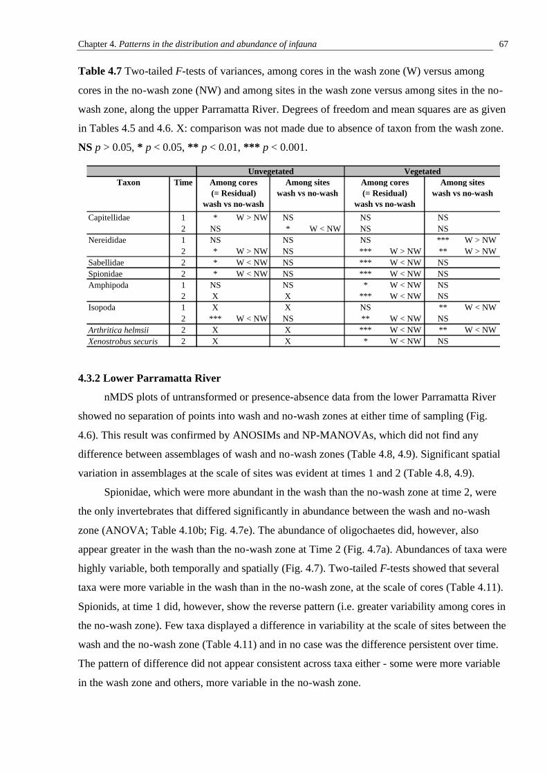
Chapter 4. Patterns in the distribution and abundance of infauna 67
Table 4.7 Two-tailed F-tests of variances, among cores in the wash zone (W) versus among
cores in the no-wash zone (NW) and among sites in the wash zone versus among sites in the no-
wash zone, along the upper Parramatta River. Degrees of freedom and mean squares are as given
in Tables 4.5 and 4.6. X: comparison was not made due to absence of taxon from the wash zone.
NS p > 0.05, * p < 0.05, ** p < 0.01, *** p < 0.001.
4.3.2 Lower Parramatta River
nMDS plots of untransformed or presence-absence data from the lower Parramatta River
showed no separation of points into wash and no-wash zones at either time of sampling (Fig.
4.6). This result was confirmed by ANOSIMs and NP-MANOVAs, which did not find any
difference between assemblages of wash and no-wash zones (Table 4.8, 4.9). Significant spatial
variation in assemblages at the scale of sites was evident at times 1 and 2 (Table 4.8, 4.9).
Spionidae, which were more abundant in the wash than the no-wash zone at time 2, were
the only invertebrates that differed significantly in abundance between the wash and no-wash
zone (ANOVA; Table 4.10b; Fig. 4.7e). The abundance of oligochaetes did, however, also
appear greater in the wash than the no-wash zone at Time 2 (Fig. 4.7a). Abundances of taxa were
highly variable, both temporally and spatially (Fig. 4.7). Two-tailed F-tests showed that several
taxa were more variable in the wash than in the no-wash zone, at the scale of cores (Table 4.11).
Spionids, at time 1 did, however, show the reverse pattern (i.e. greater variability among cores in
the no-wash zone). Few taxa displayed a difference in variability at the scale of sites between the
wash and the no-wash zone (Table 4.11) and in no case was the difference persistent over time.
The pattern of difference did not appear consistent across taxa either - some were more variable
in the wash zone and others, more variable in the no-wash zone.
Taxon Time
Capitellidae 1 * W > NW NS NS NS2 NS * W < NW NS NS
Nereididae 1 NS NS NS *** W > NW2 * W > NW NS *** W > NW ** W > NW
Sabellidae 2 * W < NW NS *** W < NW NSSpionidae 2 * W < NW NS *** W < NW NSAmphipoda 1 NS NS * W < NW NS
2 X X *** W < NW NSIsopoda 1 X X NS ** W < NW
2 *** W < NW NS ** W < NW NSArthritica helmsii 2 X X *** W < NW ** W < NWXenostrobus securis 2 X X * W < NW NS
Among cores (= Residual)
wash vs no-wash
UnvegetatedAmong sites
wash vs no-wash
VegetatedAmong sites
wash vs no-washAmong cores (= Residual)
wash vs no-wash
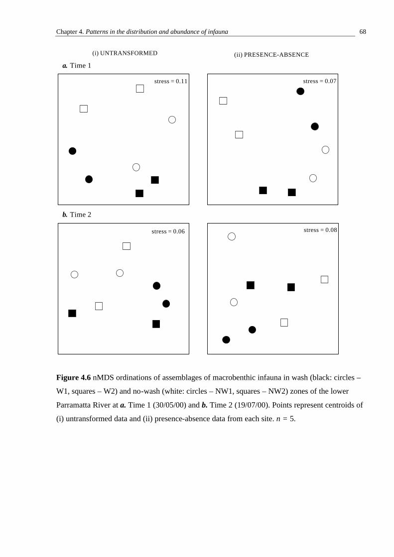
Chapter 4. Patterns in the distribution and abundance of infauna 68
Figure 4.6 nMDS ordinations of assemblages of macrobenthic infauna in wash (black: circles –
W1, squares – W2) and no-wash (white: circles – NW1, squares – NW2) zones of the lower
Parramatta River at a. Time 1 (30/05/00) and b. Time 2 (19/07/00). Points represent centroids of
(i) untransformed data and (ii) presence-absence data from each site. n = 5.
stress = 0.11
(i) UNTRANSFORMED
stress = 0.07
(ii) PRESENCE-ABSENCE
stress = 0.06 stress = 0.08
a. Time 1
b. Time 2
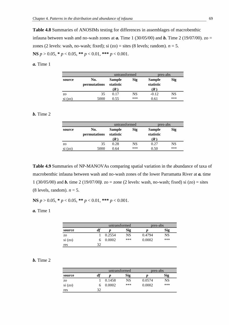
Chapter 4. Patterns in the distribution and abundance of infauna 69
Table 4.8 Summaries of ANOSIMs testing for differences in assemblages of macrobenthic
infauna between wash and no-wash zones at a. Time 1 (30/05/00) and b. Time 2 (19/07/00). zo =
zones (2 levels: wash, no-wash; fixed); si (zo) = sites (8 levels; random). n = 5.
NS p > 0.05, * p < 0.05, ** p < 0.01, *** p < 0.001.
a. Time 1
b. Time 2
Table 4.9 Summaries of NP-MANOVAs comparing spatial variation in the abundance of taxa of
macrobenthic infauna between wash and no-wash zones of the lower Parramatta River at a. time
1 (30/05/00) and b. time 2 (19/07/00). zo = zone (2 levels: wash, no-wash; fixed) si (zo) = sites
(8 levels, random). n = 5.
NS p > 0.05, * p < 0.05, ** p < 0.01, *** p < 0.001.
a. Time 1
b. Time 2
source No. permutations
Sample statistic
(R )
Sig Sample statistic
(R )
Sig
zo 35 0.17 NS -0.12 NSsi (zo) 5000 0.55 *** 0.61 ***
untransformed pres-abs
source No. permutations
Sample statistic
(R )
Sig Sample statistic
(R )
Sig
zo 35 0.28 NS 0.27 NSsi (zo) 5000 0.64 *** 0.50 ***
untransformed pres-abs
source df p Sig p Sigzo 1 0.2554 NS 0.4794 NSsi (zo) 6 0.0002 *** 0.0002 ***res 32
untransformed pres-abs
source df p Sig p Sig zo 1 0.1458 NS 0.0574 NSsi (zo) 6 0.0002 *** 0.0002 ***res 32
untransformed pres-abs
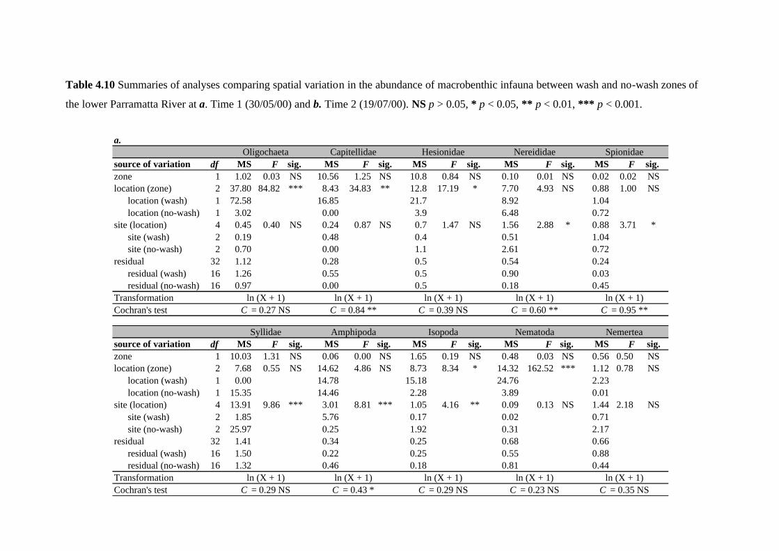
Table 4.10 Summaries of analyses comparing spatial variation in the abundance of macrobenthic infauna between wash and no-wash zones of
the lower Parramatta River at a. Time 1 (30/05/00) and b. Time 2 (19/07/00). NS p > 0.05, * p < 0.05, ** p < 0.01, *** p < 0.001.
a.
df MS F sig. MS F sig. MS F sig. MS F sig. MS F sig. zone 1 1.02 0.03 NS 10.56 1.25 NS 10.8 0.84 NS 0.10 0.01 NS 0.02 0.02 NSlocation (zone) 2 37.80 84.82 *** 8.43 34.83 ** 12.8 17.19 * 7.70 4.93 NS 0.88 1.00 NS
location (wash) 1 72.58 16.85 21.7 8.92 1.04location (no-wash) 1 3.02 0.00 3.9 6.48 0.72
site (location) 4 0.45 0.40 NS 0.24 0.87 NS 0.7 1.47 NS 1.56 2.88 * 0.88 3.71 *site (wash) 2 0.19 0.48 0.4 0.51 1.04site (no-wash) 2 0.70 0.00 1.1 2.61 0.72
residual 32 1.12 0.28 0.5 0.54 0.24residual (wash) 16 1.26 0.55 0.5 0.90 0.03residual (no-wash) 16 0.97 0.00 0.5 0.18 0.45
TransformationCochran's test
df MS F sig. MS F sig. MS F sig. MS F sig. MS F sig.zone 1 10.03 1.31 NS 0.06 0.00 NS 1.65 0.19 NS 0.48 0.03 NS 0.56 0.50 NSlocation (zone) 2 7.68 0.55 NS 14.62 4.86 NS 8.73 8.34 * 14.32 162.52 *** 1.12 0.78 NS
location (wash) 1 0.00 14.78 15.18 24.76 2.23location (no-wash) 1 15.35 14.46 2.28 3.89 0.01
site (location) 4 13.91 9.86 *** 3.01 8.81 *** 1.05 4.16 ** 0.09 0.13 NS 1.44 2.18 NSsite (wash) 2 1.85 5.76 0.17 0.02 0.71site (no-wash) 2 25.97 0.25 1.92 0.31 2.17
residual 32 1.41 0.34 0.25 0.68 0.66residual (wash) 16 1.50 0.22 0.25 0.55 0.88residual (no-wash) 16 1.32 0.46 0.18 0.81 0.44
TransformationCochran's test
ln (X + 1)C = 0.43 * C = 0.29 NS
ln (X + 1)
Isopoda
C = 0.27 NS C = 0.84 ** C = 0.39 NS
Syllidae
C = 0.95 **
Spionidaesource of variation
Amphipoda
ln (X + 1)
Oligochaeta Capitellidae Hesionidae Nereididae
Nematodasource of variation
ln (X + 1)C = 0.29 NS C = 0.35 NS
Nemertea
ln (X + 1) ln (X + 1) ln (X + 1)
ln (X + 1)ln (X + 1)
C = 0.60 **
ln (X + 1)C = 0.23 NS
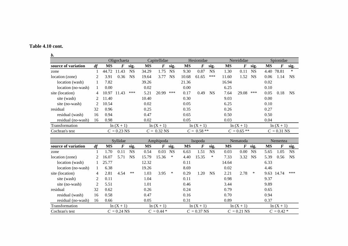
Table 4.10 cont.
b.
df MS F sig. MS F sig. MS F sig. MS F sig. MS F sig. zone 1 44.72 11.43 NS 34.29 1.75 NS 9.30 0.87 NS 1.30 0.11 NS 4.40 78.81 *location (zone) 2 3.91 0.36 NS 19.64 3.77 NS 10.68 61.65 *** 11.60 1.52 NS 0.06 1.14 NS
location (wash) 1 7.82 39.26 21.36 16.94 0.02location (no-wash) 1 0.00 0.02 0.00 6.25 0.10
site (location) 4 10.97 11.43 *** 5.21 20.99 *** 0.17 0.49 NS 7.64 29.08 *** 0.05 0.18 NSsite (wash) 2 11.40 10.40 0.30 9.03 0.00site (no-wash) 2 10.54 0.02 0.05 6.25 0.10
residual 32 0.96 0.25 0.35 0.26 0.27residual (wash) 16 0.94 0.47 0.65 0.50 0.50residual (no-wash) 16 0.98 0.02 0.05 0.03 0.04
TransformationCochran's test
df MS F sig. MS F sig. MS F sig. MS F sig. MS F sig.zone 1 1.70 0.11 NS 0.54 0.03 NS 6.63 1.51 NS 0.03 0.00 NS 5.65 1.05 NSlocation (zone) 2 16.07 5.71 NS 15.79 15.36 * 4.40 15.35 * 7.33 3.32 NS 5.39 0.56 NS
location (wash) 1 25.77 12.32 0.11 14.64 6.33location (no-wash) 1 6.38 19.26 8.69 0.02 4.46
site (location) 4 2.81 4.54 ** 1.03 3.95 * 0.29 1.20 NS 2.21 2.78 * 9.63 14.74 ***site (wash) 2 0.11 1.04 0.11 0.98 9.37site (no-wash) 2 5.51 1.01 0.46 3.44 9.89
residual 32 0.62 0.26 0.24 0.79 0.65residual (wash) 16 0.58 0.47 0.16 0.70 0.94residual (no-wash) 16 0.66 0.05 0.31 0.89 0.37
TransformationCochran's test
Spionidae
Syllidae Isopoda
Nereididae
C = 0.31 NS
Nemertea
ln (X + 1)
Capitellidae Hesionidae
ln (X + 1)
ln (X + 1)
C = 0.24 NS
Amphipoda
ln (X + 1)
C = 0.65 **
Nematoda
C = 0.21 NSln (X + 1)
source of variation
source of variation
ln (X + 1)C = 0.23 NS
Oligochaeta
C = 0.42 *
ln (X + 1)
C = 0.44 * C = 0.37 NS
C = 0.32 NS C = 0.58 **ln (X + 1)
ln (X + 1)ln (X + 1)
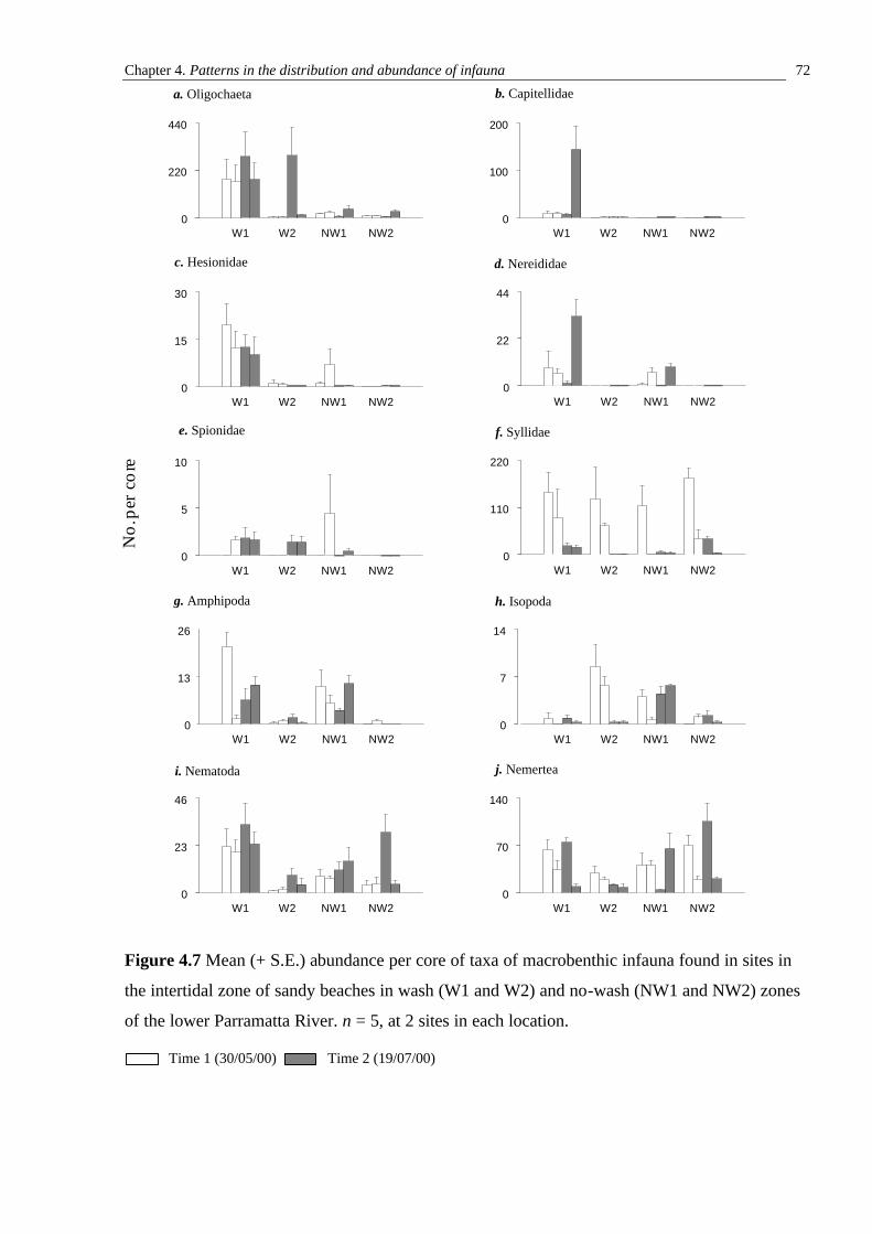
Chapter 4. Patterns in the distribution and abundance of infauna 72
Figure 4.7 Mean (+ S.E.) abundance per core of taxa of macrobenthic infauna found in sites in
the intertidal zone of sandy beaches in wash (W1 and W2) and no-wash (NW1 and NW2) zones
of the lower Parramatta River. n = 5, at 2 sites in each location.
Time 1 (30/05/00) Time 2 (19/07/00)
W1 W2 NW1 NW20
220
440
a. Oligochaeta
W1 W2 NW1 NW20
100
200
b. Capitellidae
W1 W2 NW1 NW20
15
30
c. Hesionidae
W1 W2 NW1 NW20
22
44
d. Nereididae
W1 W2 NW1 NW20
5
10
e. Spionidae
W1 W2 NW1 NW20
110
220
f. Syllidae
W1 W2 NW1 NW20
13
26
g. Amphipoda
W1 W2 NW1 NW20
7
14
h. Isopoda
W1 W2 NW1 NW20
23
46
i. Nematoda
W1 W2 NW1 NW20
70
140
j. Nemertea
No.
per
core
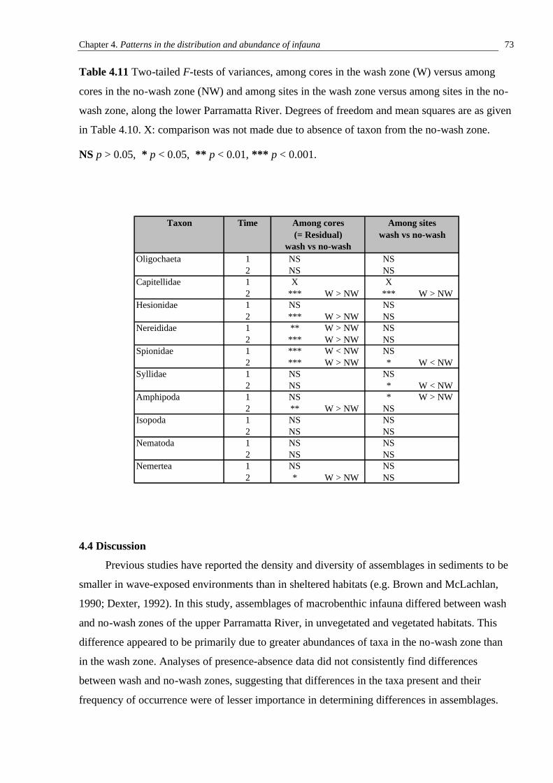
Chapter 4. Patterns in the distribution and abundance of infauna 73
Table 4.11 Two-tailed F-tests of variances, among cores in the wash zone (W) versus among
cores in the no-wash zone (NW) and among sites in the wash zone versus among sites in the no-
wash zone, along the lower Parramatta River. Degrees of freedom and mean squares are as given
in Table 4.10. X: comparison was not made due to absence of taxon from the no-wash zone.
NS p > 0.05, * p < 0.05, ** p < 0.01, *** p < 0.001.
4.4 Discussion
Previous studies have reported the density and diversity of assemblages in sediments to be
smaller in wave-exposed environments than in sheltered habitats (e.g. Brown and McLachlan,
1990; Dexter, 1992). In this study, assemblages of macrobenthic infauna differed between wash
and no-wash zones of the upper Parramatta River, in unvegetated and vegetated habitats. This
difference appeared to be primarily due to greater abundances of taxa in the no-wash zone than
in the wash zone. Analyses of presence-absence data did not consistently find differences
between wash and no-wash zones, suggesting that differences in the taxa present and their
frequency of occurrence were of lesser importance in determining differences in assemblages.
Taxon Time
Oligochaeta 1 NS NS2 NS NS
Capitellidae 1 X X2 *** W > NW *** W > NW
Hesionidae 1 NS NS2 *** W > NW NS
Nereididae 1 ** W > NW NS2 *** W > NW NS
Spionidae 1 *** W < NW NS2 *** W > NW * W < NW
Syllidae 1 NS NS2 NS * W < NW
Amphipoda 1 NS * W > NW2 ** W > NW NS
Isopoda 1 NS NS2 NS NS
Nematoda 1 NS NS2 NS NS
Nemertea 1 NS NS2 * W > NW NS
Among cores (= Residual)
wash vs no-wash
Among sites wash vs no-wash
Chapter 4. Patterns in the distribution and abundance of infauna 74
The effect of wash on infaunal assemblages did not, however, appear general. In the lower
Parramatta River, no difference was found between the assemblages of wash and no-wash zones.
The difference between assemblages in wash and no-wash zones of the upper Parramatta
River was smaller in the vegetated than in the unvegetated habitat at the first time of sampling.
At time 2, however, a similar difference was seen between the wash and the no-wash zone in
each of the habitats. Bray-Curtis dissimilarities between the assemblages of the unvegetated and
vegetated habitats were greater for sites in the wash zone than in the no-wash zone at each time.
This may, however, be attributed to the greater within-site variability in assemblages in the no-
wash, in each of the habitats. Thus, it remains unclear whether the root structure of mangroves
indeed reduces the impact of boat-generated waves on infaunal assemblages.
In contrast to previous studies (e.g. Plazait, 1975; Wells, 1986; Sheridan, 1997) no obvious
difference in the abundance and number of taxa present in the unvegetated and vegetated habitat
was evident. Assemblages in the upper Parramatta River were fairly depauperate and were
dominated by the opportunistic families of polychaetes, Capitellidae, Nereididae and Spionidae.
The greater abundance of these three taxa and of Amphipoda, Isopoda and Xenostrobus securis
in the no-wash than in the wash zone of the upper Parramatta River were primarily responsible
for the difference detected between the assemblages of these two places. At time 2, smaller
numbers of Nephytiidae in the no-wash zone than the wash zone may also have contributed to
this pattern.
It has been hypothesised that disturbances, such as wind-stresses, that decrease the stability
of the sediment, result in assemblages dominated by deposit-feeders and in which filter-feeders
have a proportionally small abundance (Rhoads, 1974; Wildish and Peer, 1983; Wildish and
Kristmanson, 1997). The preponderance of deposit-feeders in assemblages of the upper
Parramatta River, however, is probably unrelated to the disturbance of sediment by RiverCat
wash. Previous studies have found opportunistic deposit-feeders to dominate estuarine waters
(e.g. Pearson and Rosenberg, 1978; Schaffner et al., 1987) and muddy sediments such as those
found along the upper Parramatta River (e.g. Rhoads, 1974; Rhoads and Young, 1970). The great
abundance of suspension-feeders along the lower Parramatta River, also exposed to wash but
with sandy sediment and a greater salinity, suggests that this is the case.
Underwood (1991, 1992, 1993, 1994) has drawn attention to the fact that, rather than
simply altering abundances, impacts may alter temporal and spatial variability in impacted
locations compared with control locations. Assemblages in wash or no-wash zones of the upper
and lower Parramatta River were highly variable, spatially and temporally. In the upper
Parramatta River, within-site variability in assemblages was generally smaller for sites in the no-

Chapter 4. Patterns in the distribution and abundance of infauna 75
wash zone than for sites in the wash zone in unvegetated and vegetated habitat. This supports
Warwick and Clarke’s (1993) model that increased variability is a symptom of stressed
environments. When spatial variability was examined for individual taxa, however, the reverse
pattern was generally seen. The greater variability in the abundance of individual taxa in no-
wash may be a function of the greater mean abundances found there.
The different patterns found between wash and no-wash zones of the upper and lower
Parramatta River are not surprising considering the many differences found between these two
sections of the river. While the number of RiverCats travelling on each of these sections of river
was very similar, the main river channel is 2-3 times wider near the Gladesville Bridge than
adjacent to the Silverwater Bridge. Thus, the intensity of wash from RiverCats reaching the
shore should be smaller along the lower Parramatta River than along its upper reaches (see Das
and Johnson, 1970; Bhowmik, 1975). The width of the lower Parramatta River also means that
there is a greater available fetch for the generation of wind-driven waves. Coupled with the great
recreational boat-traffic at the Gladesville Bridge, which is more than four times that at
Silverwater (Patterson Britton, 2000b), these waves may swamp any effect of wash from
RiverCat ferries along the lower Parramatta River.
It also appears that compliance with the no-wash regulation is greater at the upstream no-
wash zone than at the downstream zone. Data collected by NSW Waterways on the speed of
RiverCat ferries at various points along the river indicate that, while the majority of ferries slow
to within the 7 knot speed-limit upon entering the upstream no-wash zone, most vessels maintain
their speed (which may be as great as 30 knots) upon entering the downstream no-wash zone
(Patterson Britton, 2000a). This is not surprising considering drivers may be fined for exceeding
the speed limit in the upper no-wash zone, but are not given a suggested speed limit for the
downstream no-wash zone.
Although the no-wash zone located to the west of the Silverwater Bridge appears to be
important in reducing the impact of ferry-wash on macrobenthic infauna, the experimental
design used to examine differences between the assemblages of the wash and no-wash zone is
potentially confounded. Potential sources of confounding include: (i) gradients in variables, such
as salinity, which occur along rivers with distance from the sea, (ii) differences in the
concentration of contaminants in the sediment adjacent to locations differing in their historic
land-use, (iii) the exclusion of recreational boat traffic from the section of the Parramatta River
to the west of the Silverwater Bridge and (iv) intrinsic differences between the two sections of
river.
Chapter 4. Patterns in the distribution and abundance of infauna 76
Gradients in salinity and nutrients are important in determining the distribution and
abundance of macrobenthic infauna (Boesch, 1977; Zajac and Whitlatch, 1982a; Schaffner et al.,
1987; de Decker and Bally, 1985; Castel et al., 1989; Junoy and Vieitez, 1990). The results of
this study do not, however, appear to be confounded by gradients along the river. As shown by
Figure 4.5, in which locations are ordered in terms of their geographical location, patterns in the
abundance of taxa do not follow a gradient with distance.
Similarly, patterns in the abundance of taxa do not appear to follow the likely pattern of
contaminants. Numerous studies have shown the abundance of deposit-feeding polychaetes to be
greater in places exposed to large concentrations of organic and toxic contaminants than places
where the concentration of these is less (e.g. Gray et al., 1988; Gray et al., 1990; Warwick and
Clarke, 1993; Braddock et al., 1995). The abundances of small crustaceans, such as amphipods
and isopods are negatively correlated with the concentration of toxic chemicals (e.g. Stander and
Venter, 1968; Notini, 1978; Lenihan and Oliver, 1995). Amphipods and isopods were less
abundant at the location situated adjacent to Wilson Park, a site formally occupied by the
Petroleum and Chemical Corporation Austalia Ltd. (1954-1974), and, hence, conformed to the
above pattern. The abundance of deposit-feeding polychaetes (Capitellidae) was, however, also
less at this location and, hence, followed the reverse pattern to that which would be expected
from previous observations.
The remaining two potential sources of confounding cannot, unfortunately, be ruled out.
The coincident location of the no-wash zone and the section of the river closed to recreational
boating means that the difference observed between wash and no-wash zones may have been due
to a difference in the volume of boat traffic between the two areas and not due to any difference
in the intensity of wash from the RiverCats. During sampling, few boats were, however,
observed adjacent to the places sampled in the wash zone, they were generally small and
produced negligible amounts of wash compared to the RiverCats.
The fact that it was decided to establish a no-wash zone to the west of the Silverwater
Bridge suggests that differences exist between the two sections of the river making the section to
the west of the Silverwater Bridge more susceptible to the effects of wash and the section to the
east less susceptible. A sampling design where assemblages are compared between times when
the ferries are in operation and times when the ferries are stopped is required for causation to be
established. Such a sampling regime is described in Chapter 5.
Thus, it appears that no-wash zones may be effective in reducing the impact of wash on the
ecology of intertidal macrobenthic infauna and the morphology of river banks in places in places
where compliance with this regulation is great. A few violations may, however, result in a
Chapter 4. Patterns in the distribution and abundance of infauna 77
significant impact on the intertidal zone. The difference between assemblages in wash and no-
wash zones does not appear to be smaller in pneumatophore than unvegetated habitat.
Mangroves may, however, be found to be important in reducing the effects of boat-wash on
macrobenthic infauna in places where the impact is greater (i.e. when places completely
sheltered from wash and places that are very exposed are compared).
CHAPTER 5
THE 2000 SYDNEY OLYMPIC GAMES: GOOD FOR SPORT AND MACROFAUNA?
5.1 Introduction
Despite the plethora of studies that have invoked wave-action to explain patterns in the
distribution and abundance of taxa of macrobenthic infauna (discussed in Section 4.1), few have
attempted to demonstrate unambiguously a causal relationship between these variables.
Surveying the plants and animals present in sheltered or exposed sites provides little insight into
the processes causing any difference in assemblages between the two exposures. A difference
between assemblages could be due to factors other than wave-action.
Manipulative experiments are the best way to determine the processes that cause spatial
and temporal patterns of variation (see Underwood, 1990). In the case of environmental impacts,
these usually take the form of a before-after study (see Underwood 1992, 1993, 1994), the
manipulation being the disturbance itself. There are many instances where it is, however,
impossible to obtain sufficient ‘before’ data to do a BACI or beyond-BACI style analysis. For
example, oil-spills usually occur without any prior indication and there is usually insufficient
time to collect samples between weather warnings and major storms.
A number of strategies has been used to demonstrate causation where there are no ‘before’
data. The first of these involves introducing artificial substrata (e.g. settlement panels,
defaunated sediment) to the putatively impacted site and control sites to test for any difference in
the assemblages that recolonise the substrata between the two types of area (Glasby and
Underwood, 1996). This method assumes that the effect of the disturbance is sustained over time
(i.e. it has a press response) and will not be useful if the assemblage has a pulse response to the
disturbance.
The second method involves determining whether assemblages of the putatively impacted
site recover following the removal of the impact (e.g. Rosenberg, 1972; Friberg et al., 1998).
This method will be useful as long as assemblages are not permanently altered by the
disturbance.
In Chapter 4, it was found that assemblages of macrobenthic infauna differed between
wash and no-wash zones of the upper Parramatta River. It was not possible, however, to
determine whether this pattern was directly caused by wash from RiverCat ferries or was due to
some other factor, because no data were available from prior to the commencement of services.
During the Sydney Olympic Games, in September, 2000, RiverCat ferry services to the west of
Homebush Bay were suspended for 5 weeks. If the patterns described in Chapter 4 were indeed
Chapter 5. The 2000 Sydney Olympic Games: Good for sport and macrofauna? 79
due to wash from RiverCat ferries, recovery of assemblages, impacted by wash, may occur over
this period of time. Therefore, it was predicted that assemblages in wash zones, where the
intensity of the disturbance is believed to be greatest, would change to become more similar to
those in no-wash zones following the suspension of services and change back to their disturbed
state following the return of ferries. It was also predicted that any change in response to the
cessation of ferry services seen in the assemblages of the no-wash zone would be smaller than
that seen in assemblages of the wash zone.
In Chapter 4, it was also found that the abundances of capitellids, nereids, spionids and
amphipods were greater in the no-wash zone than the wash zone, in each of the habitats. If these
patterns are due to wash, the abundances of these taxa in the wash zone should increase
following the suspension of ferry services and decrease following the return of services. Any
change to abundances in the no-wash zone should be less than in the no-wash zone.
5.2 Materials and Methods
RiverCat ferry services were temporarily suspended to the west of Homebush Bay from the
28th August - 2nd October, 2000. The area affected by the stoppage included both the upstream
wash and no-wash zones previously sampled (Fig. 5.1). Services to the east of Homebush Bay
continued to operate during this time.
In order to test the above hypotheses, macrobenthic infauna were sampled in unvegetated
and vegetated habitat in two locations within the upstream no-wash zone (Silverwater Park,
Silverwater [NW1] and 500 m east of Rydalmere Wharf, Rydalmere [NW2 – referred to as
NW/NW3 in Chapter 4]), two locations within the wash zone (George Kendall Reserve,
Ermington [W1] and Wilson Park, Silverwater [W2]) and two locations to the east of Homebush
Bay (control locations; Settlers Park, Putney [C1] and Shepherd’s Bay, Meadowbank [C2]; Fig.
5.1) at two times during the suspension of services (6th September 2000 [time 4] and 25th
September [time 5], 2000) and two times after the re-introduction of services (26th October, 2000
[time 5] and 10th February, 2001 [time 6]).
At each time of sampling, 5 cores of sediment were collected from each of two sites in the
unvegetated habitat and vegetated habitat using the method described in Section 4.2. The
samples collected from wash and no-wash zones on 28th April, 2000 (time 1) and 30th May, 2000
(time 2; Chapter 4) were used as ‘before-data’. Unfortunately, no data were collected from
control locations at times 1 and 2 since the suspension of services was only publicized shortly
before its commencement.
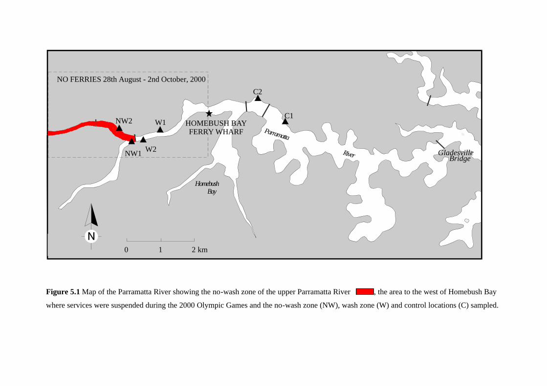
Figure 5.1 Map of the Parramatta River showing the no-wash zone of the upper Parramatta River , the area to the west of Homebush Bay
where services were suspended during the 2000 Olympic Games and the no-wash zone (NW), wash zone (W) and control locations (C) sampled.
Parramatta
River
HomebushBay
W1
W2
NW2
NW1
0 2 km1
GladesvilleBridge
C1
C2
HOMEBUSH BAYFERRY WHARF
NO FERRIES 28th August - 2nd October, 2000
Chapter 5. The 2000 Sydney Olympic Games: Good for sport and macrofauna? 81
Data collected from the unvegetated and vegetated habitats were analysed separately
because the results presented in Chapter 4 suggested that the abundances of taxa differ between
these. NP-MANOVAs were done on untransformed data to test the hypothesis of a significant
site x time interaction, as would be expected if assemblages in the wash zone were more
disturbed than were those in the no-wash zone (change following the removal of the disturbance
should be greatest in the most impacted places). Because NP-MANOVAs can only handle two
factors and sites within some locations contained very different assemblages, differences among
locations were omitted from many of the analyses to leave the two factors, time and site.
Presence-absence data were not analysed because the results in Chapter 4 suggested that any
difference between wash and no-wash zones were primarily due to differences in the abundances
of taxa and not due to differences in the taxa present or the number of cores occupied.
The results in Chapter 4 indicated that within-site variability in assemblages was less in the
no-wash zone than in the wash zone. A model to explain this pattern is that disturbance by wash
is the real cause of increases in the spatial variability of assemblages at this scale. Bray-Curtis
measures of variability within sites of the wash and no-wash zone were compared to test the
corresponding hypotheses that variability within sites of the wash zone would: (i) decrease
following the removal of the disturbing force and (ii) increase again following its return. It was
also hypothesized that less change would occur in the no-wash zone than the wash zone.
5.3 Results
5.3.1 Multivariate changes
Sorting of samples from control locations at times 3 and 4 indicated that their assemblages
of macrobenthic fauna were very different from those from the wash or no-wash zone (Fig. 5.2).
Differences were evident when assemblages of the control locations (at times 3 and 4) were
compared to those in the wash or no-wash zone at times when the ferries were running (1 and 2;
Fig. 5.2a). They were also evident in comparisons among assemblages of wash, no-wash and
control sites, in the unvegetated and the vegetated habitat, during the suspension of services (Fig.
5.2b,c; Table 5.1). In both the unvegetated and the vegetated habitats, the abundances of
oligochaetes and polychaetes of the family, Nephytiidae, were much greater in controls than at
the other places. The abundances of sabellid polychaetes were also greater at control locations
within the unvegetated habitat.
Given that the assemblages in control locations did not appear representative of the
assemblages in wash or no-wash zones, at times before or during the cessation, it was decided
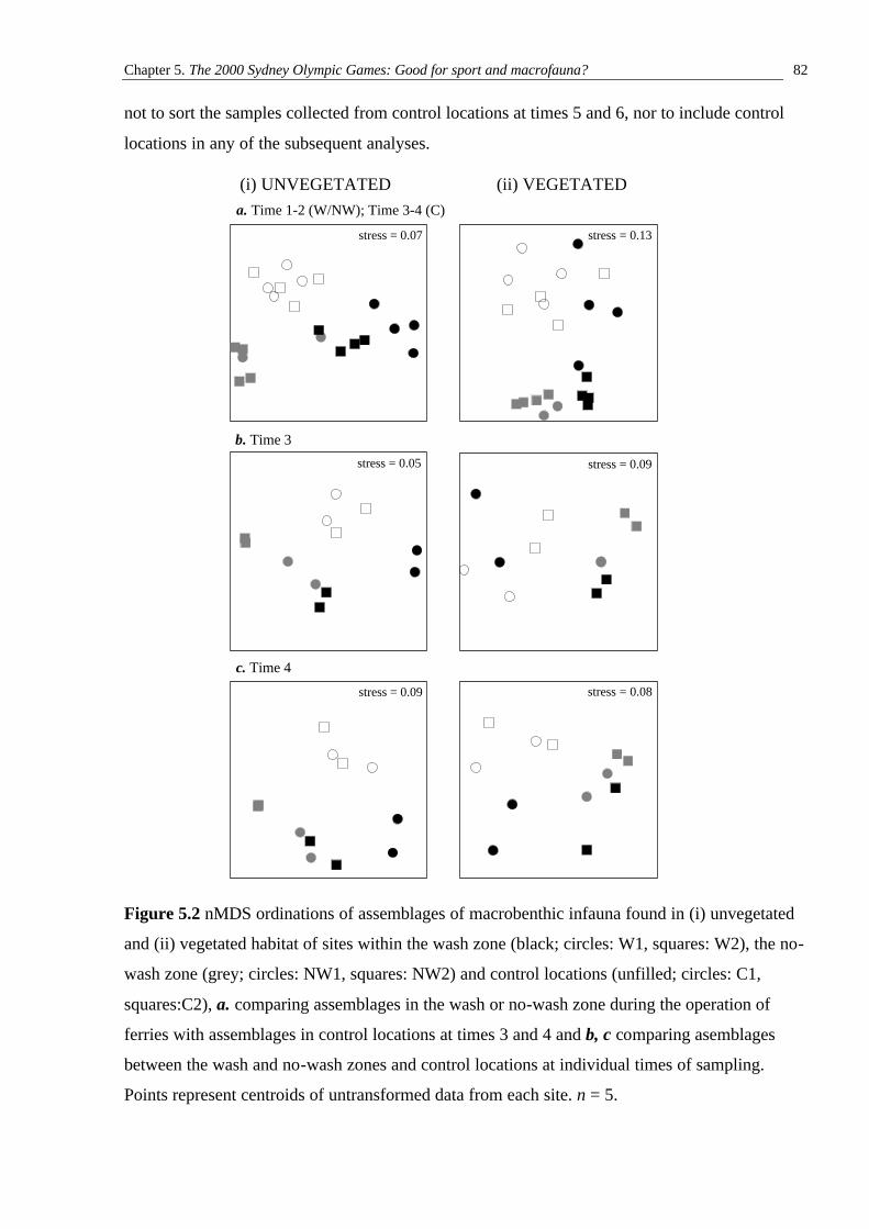
Chapter 5. The 2000 Sydney Olympic Games: Good for sport and macrofauna? 82
stress = 0.07 stress = 0.13
stress = 0.05 stress = 0.09
stress = 0.09 stress = 0.08
b. Time 3
c. Time 4
a. Time 1-2 (W/NW); Time 3-4 (C)
not to sort the samples collected from control locations at times 5 and 6, nor to include control
locations in any of the subsequent analyses.
Figure 5.2 nMDS ordinations of assemblages of macrobenthic infauna found in (i) unvegetated
and (ii) vegetated habitat of sites within the wash zone (black; circles: W1, squares: W2), the no-
wash zone (grey; circles: NW1, squares: NW2) and control locations (unfilled; circles: C1,
squares:C2), a. comparing assemblages in the wash or no-wash zone during the operation of
ferries with assemblages in control locations at times 3 and 4 and b, c comparing asemblages
between the wash and no-wash zones and control locations at individual times of sampling.
Points represent centroids of untransformed data from each site. n = 5.
(i) UNVEGETATED (ii) VEGETATED
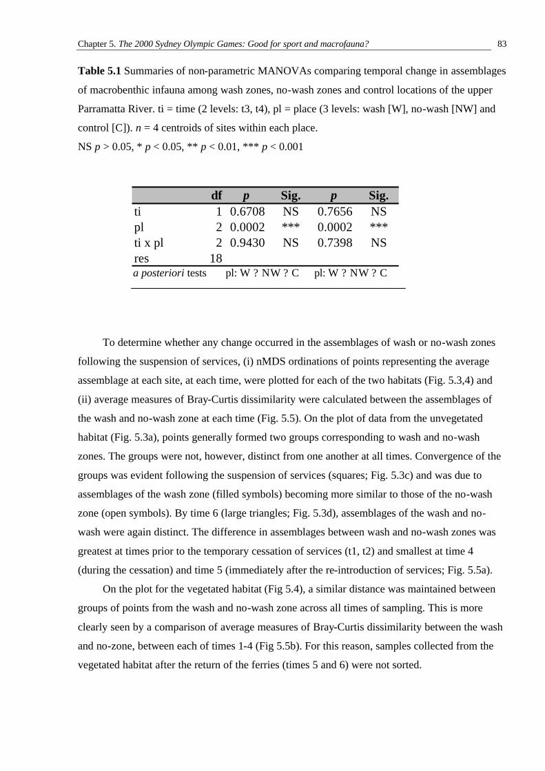
Chapter 5. The 2000 Sydney Olympic Games: Good for sport and macrofauna? 83
Table 5.1 Summaries of non-parametric MANOVAs comparing temporal change in assemblages
of macrobenthic infauna among wash zones, no-wash zones and control locations of the upper
Parramatta River. ti = time (2 levels: t3, t4), pl = place (3 levels: wash [W], no-wash [NW] and
control [C]). n = 4 centroids of sites within each place.
NS p > 0.05, * p < 0.05, ** p < 0.01, *** p < 0.001
a posteriori tests pl: W ? NW ? C pl: W ? NW ? C
To determine whether any change occurred in the assemblages of wash or no-wash zones
following the suspension of services, (i) nMDS ordinations of points representing the average
assemblage at each site, at each time, were plotted for each of the two habitats (Fig. 5.3,4) and
(ii) average measures of Bray-Curtis dissimilarity were calculated between the assemblages of
the wash and no-wash zone at each time (Fig. 5.5). On the plot of data from the unvegetated
habitat (Fig. 5.3a), points generally formed two groups corresponding to wash and no-wash
zones. The groups were not, however, distinct from one another at all times. Convergence of the
groups was evident following the suspension of services (squares; Fig. 5.3c) and was due to
assemblages of the wash zone (filled symbols) becoming more similar to those of the no-wash
zone (open symbols). By time 6 (large triangles; Fig. 5.3d), assemblages of the wash and no-
wash were again distinct. The difference in assemblages between wash and no-wash zones was
greatest at times prior to the temporary cessation of services (t1, t2) and smallest at time 4
(during the cessation) and time 5 (immediately after the re-introduction of services; Fig. 5.5a).
On the plot for the vegetated habitat (Fig 5.4), a similar distance was maintained between
groups of points from the wash and no-wash zone across all times of sampling. This is more
clearly seen by a comparison of average measures of Bray-Curtis dissimilarity between the wash
and no-zone, between each of times 1-4 (Fig 5.5b). For this reason, samples collected from the
vegetated habitat after the return of the ferries (times 5 and 6) were not sorted.
df p Sig. p Sig.ti 1 0.6708 NS 0.7656 NSpl 2 0.0002 *** 0.0002 ***ti x pl 2 0.9430 NS 0.7398 NSres 18
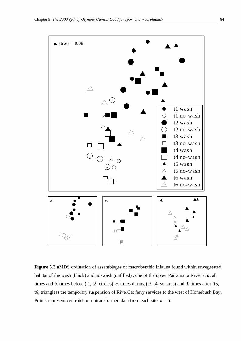
Chapter 5. The 2000 Sydney Olympic Games: Good for sport and macrofauna? 84
Figure 5.3 nMDS ordination of assemblages of macrobenthic infauna found within unvegetated
habitat of the wash (black) and no-wash (unfilled) zone of the upper Parramatta River at a. all
times and b. times before (t1, t2; circles), c. times during (t3, t4; squares) and d. times after (t5,
t6; triangles) the temporary suspension of RiverCat ferry services to the west of Homebush Bay.
Points represent centroids of untransformed data from each site. n = 5.
stress = 0.08
t1 washt1 no-washt2 washt2 no-washt3 washt3 no-washt4 washt4 no-washt5 washt5 no-washt6 washt6 no-wash
d.
a. stress = 0.08
b. c.
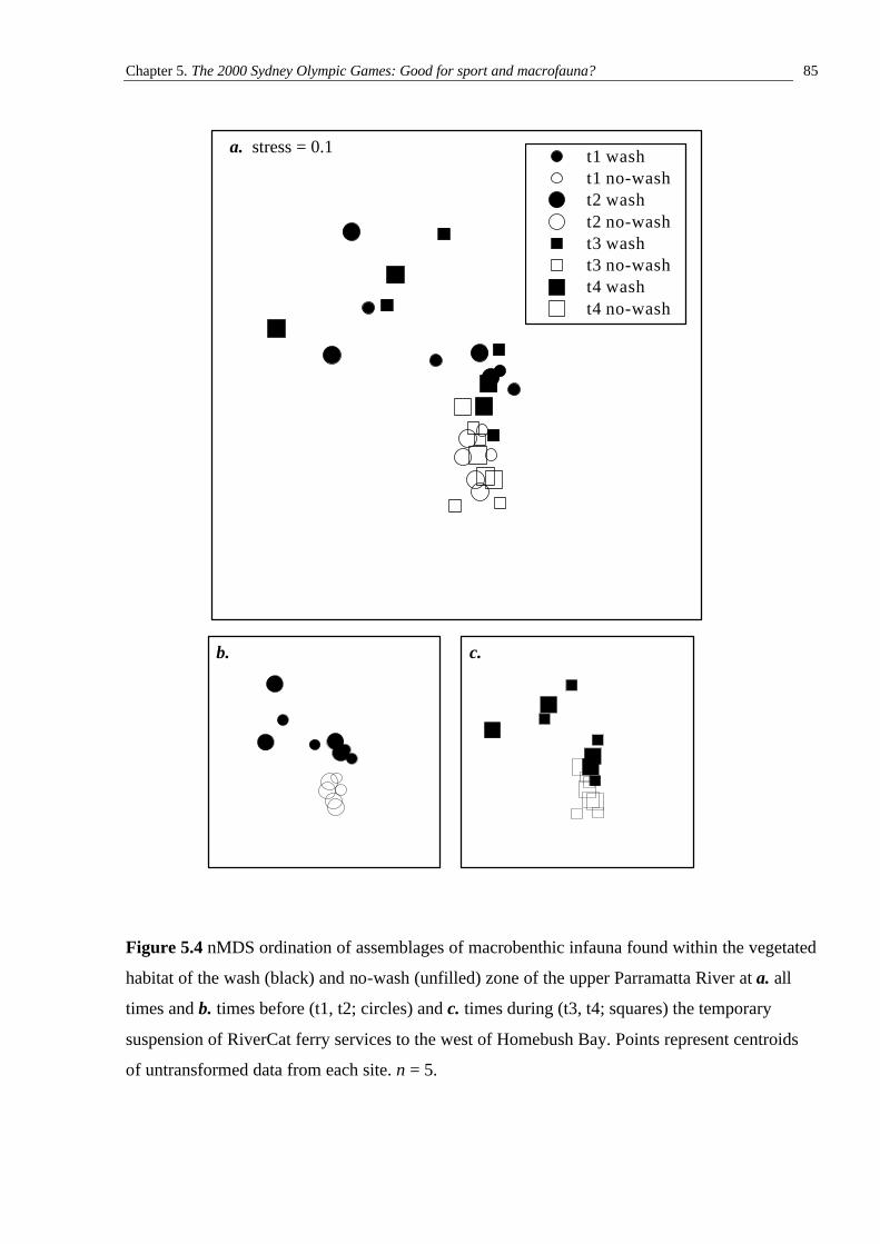
Chapter 5. The 2000 Sydney Olympic Games: Good for sport and macrofauna? 85
Figure 5.4 nMDS ordination of assemblages of macrobenthic infauna found within the vegetated
habitat of the wash (black) and no-wash (unfilled) zone of the upper Parramatta River at a. all
times and b. times before (t1, t2; circles) and c. times during (t3, t4; squares) the temporary
suspension of RiverCat ferry services to the west of Homebush Bay. Points represent centroids
of untransformed data from each site. n = 5.
a. stress = 0.1
b. c.
t1 washt1 no-washt2 washt2 no-washt3 washt3 no-washt4 washt4 no-wash
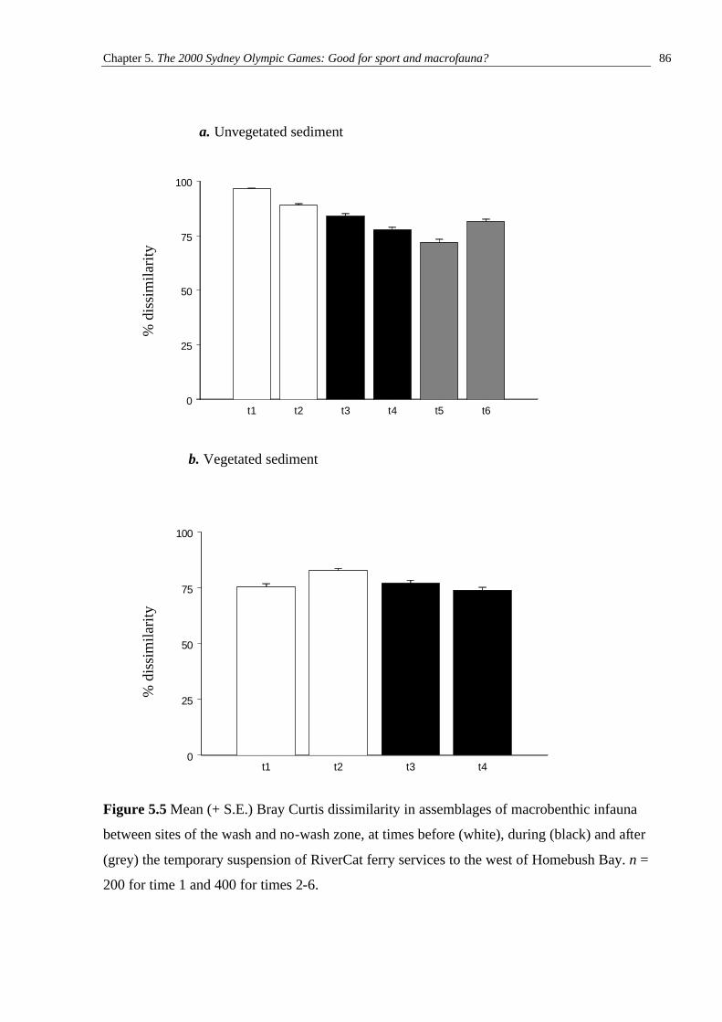
Chapter 5. The 2000 Sydney Olympic Games: Good for sport and macrofauna? 86
Figure 5.5 Mean (+ S.E.) Bray Curtis dissimilarity in assemblages of macrobenthic infauna
between sites of the wash and no-wash zone, at times before (white), during (black) and after
(grey) the temporary suspension of RiverCat ferry services to the west of Homebush Bay. n =
200 for time 1 and 400 for times 2-6.
t1 t2 t3 t4 t5 t60
25
50
75
100
t1 t2 t3 t40
25
50
75
100
a. Unvegetated sediment
b. Vegetated sediment
% d
issi
mila
rity
% d
issi
mila
rity
Chapter 5. The 2000 Sydney Olympic Games: Good for sport and macrofauna? 87
Patterns of change in the assemblages of the unvegetated habitat were further examined
through separate ordinations of the data from each site (Figure 5.6). These enabled the temporal
change within each site to be seen without distortion of the plot by points from the other sites.
These plots show that, within the wash zone, three of the four sites changed following the
removal of ferries (shortly after time 2) and became more similar to their initial state following
the return of services (times 5 and 6; Fig. 5.6b,c,d). The assemblage at the fourth site, W1(S1),
changed randomly (Fig. 5.6a). Similar patterns were not generally found among plots of data
from the no-wash zone. The assemblage at NW1(S1) became increasingly different from its
original composition throughout the study (Fig. 5.6e). The assemblage at NW1(S2) displayed a
similar pattern of change to sites in the wash zone (Fig. 5.6f). Sites at NW2 followed a cyclic
pattern of change between times 1 and 5, consistent with the removal and return of ferry services
(Fig. 5.6 g,h). Between times 5 and 6, however, assemblages changed to become very different
in composition from every other time.
Spearman’s rank correlations were done between the matrix of Bray-Curtis dissimilarities
for each site, calculated using samples from all times, and a matrix of ranks corresponding to a
pattern of cyclic change (RELATE, Clarke and Warwick, 2001; Table 5.2). These were to test
the hypothesis that the pattern of change would be cyclic (i.e. change away from, and then back
towards, the starting point) at sites of the wash zone but not at sites of the no-wash zone. The
correlation at W2(S2) was significant.
In order to compare patterns of temporal change among sites, in the unvegetated habitat,
second stage nMDS ordinations (Somerfield and Clarke, 1995) were done (Fig. 5.7). The
proximity of points (representing sites) on these ordinations indicates the extent to which
different sites display the same temporal pattern of change. Two ordinations were done because
the two sites at NW1 were not sampled at time 1. The first compared six sites (W1(S1), W1(S2),
W2(S1), W2(S2), NW2(S1), NW2(S2)) across all (6) times of sampling (Fig. 5.7(a) and the
other compared all sites (including NW1(S1) and NW1(S2)) across five times of sampling (times
2-6; Fig. 5.7b). The second-stage nMDS for temporal change in the six sites across all times
showed the pattern within sites at NW2 to be very different from that in sites in the wash zone
(Fig. 5.7a). W1(S1) did not, however, conform to the general pattern of change seen among the
sites of the wash zone. When change at all sites was considered across five times of sampling,
points did not separate into distinct groups. Sites within the no-wash zone did, however,
generally display patterns of change that were more similar to one another than to the patterns in
sites in the wash zone. The exception was NW1(S2), which appeared to have an identical pattern
of change to W2(S1), according to the nMDS.
Chapter 5. The 2000 Sydney Olympic Games: Good for sport and macrofauna? 88
Two way NP-MANOVAs, with the factors time and site, were done on the data from the
unvegetated habitat to test for a time x site interaction, which may be indicative of differing
responses of the assemblages of wash and no-wash zones to the removal of the disturbance.
Unfortunately the factors wash, location and period (before, after, during the cessation) could not
be included in the analyses because NP-MANOVAs can only deal with two factors at a time.
These analyses included all eight of the sites sampled (W1(S1), W1(S2), W2(S1), W2(S2),
NW1(S1), NW1(S2), NW2(S1), NW2(S2)) and included five of the sampling times (2-6). Time
1 was omitted from analyses because there were no data available for the two sites at NW1, at
this time. A significant time x site interaction was found (Table 5.3). A posteriori tests indicated
that the pattern of temporal change was very variable among sites in the wash zone. In the no-
wash zone, however, similar assemblages were generally found between times 3 and 4, with very
different assemblages at times 2 and 6.
In the wash zone, variability was greatest at times prior to the cessation of services (Fig.
5.8; t1, t2: white bars) and at time 6, after the return of services. Variability was smallest at times
4 and 5. In the no-wash zone, the pattern of change was not consistent with the temporary
cessation of services. Dissimilarity was greatest at time 6 and smallest at time 1.
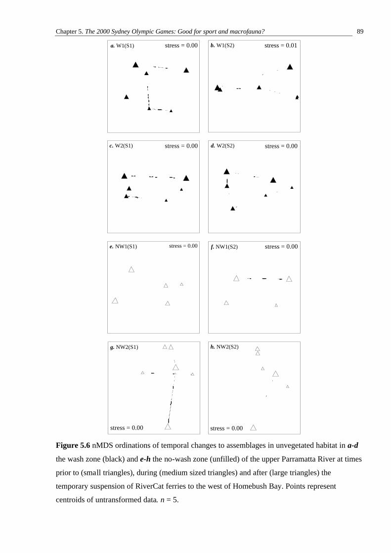
Chapter 5. The 2000 Sydney Olympic Games: Good for sport and macrofauna? 89
a. W1(S1) stress = 0.00
Figure 5.6 nMDS ordinations of temporal changes to assemblages in unvegetated habitat in a-d
the wash zone (black) and e-h the no-wash zone (unfilled) of the upper Parramatta River at times
prior to (small triangles), during (medium sized triangles) and after (large triangles) the
temporary suspension of RiverCat ferries to the west of Homebush Bay. Points represent
centroids of untransformed data. n = 5.
b. W1(S2) stress = 0.01
c. W2(S1) stress = 0.00 d. W2(S2) stress = 0.00
f. NW1(S2) stress = 0.00
g. NW2(S1)
stress = 0.00
h. NW2(S2)
stress = 0.00
stress = 0.00e. NW1(S1)
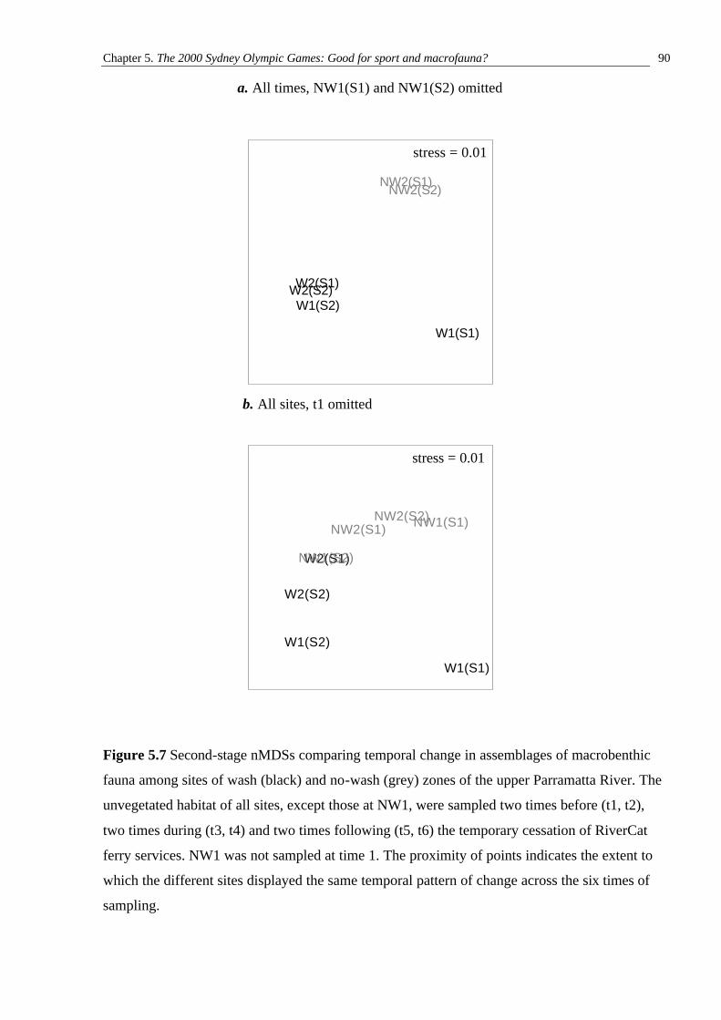
Chapter 5. The 2000 Sydney Olympic Games: Good for sport and macrofauna? 90
Figure 5.7 Second-stage nMDSs comparing temporal change in assemblages of macrobenthic
fauna among sites of wash (black) and no-wash (grey) zones of the upper Parramatta River. The
unvegetated habitat of all sites, except those at NW1, were sampled two times before (t1, t2),
two times during (t3, t4) and two times following (t5, t6) the temporary cessation of RiverCat
ferry services. NW1 was not sampled at time 1. The proximity of points indicates the extent to
which the different sites displayed the same temporal pattern of change across the six times of
sampling.
a. All times, NW1(S1) and NW1(S2) omitted
b. All sites, t1 omitted
W1(S1)
W1(S2)
W2(S1)W2(S2)
NW2(S1)NW2(S2)
stress = 0.01
W1(S1)
W1(S2)
W2(S1)
W2(S2)
NW1(S1)
NW1(S2)
NW2(S1)NW2(S2)
stress = 0.01
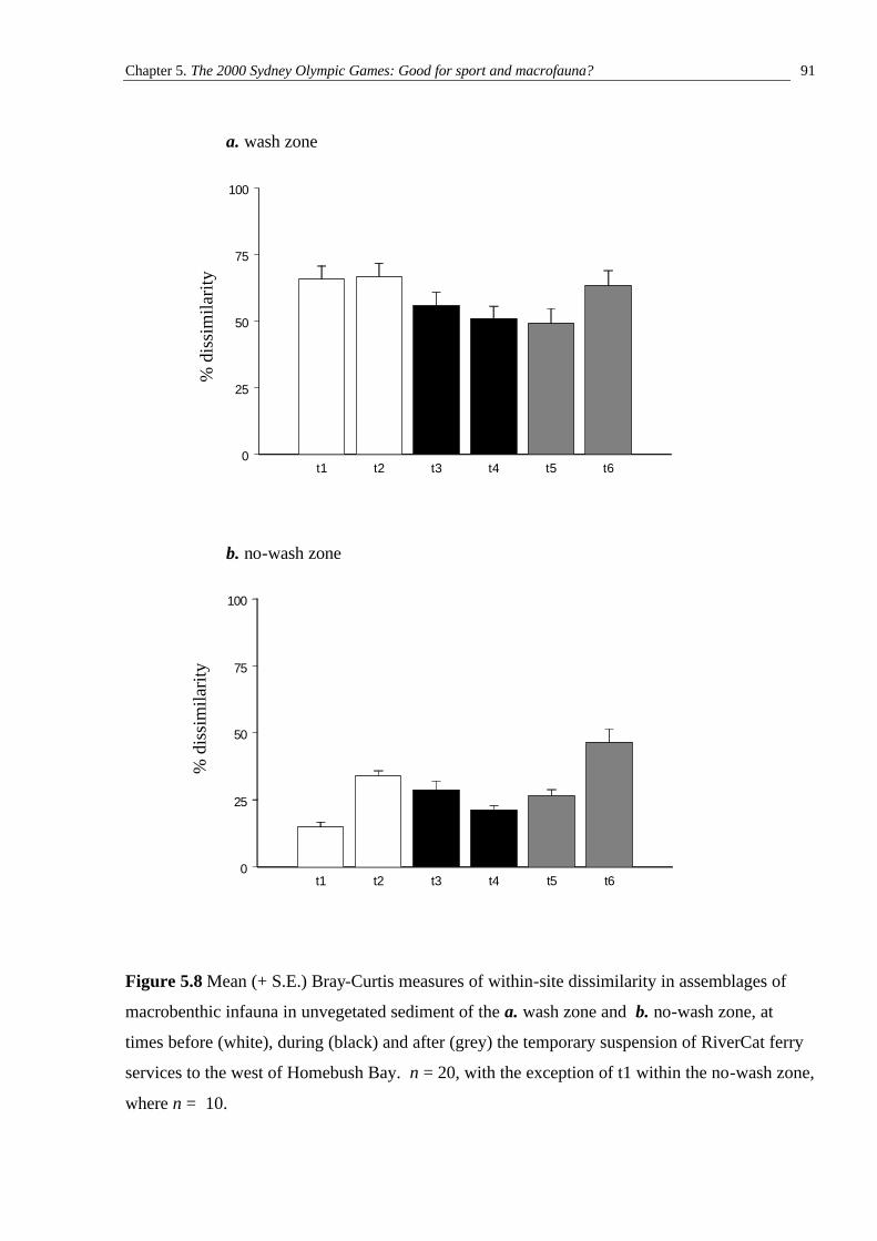
Chapter 5. The 2000 Sydney Olympic Games: Good for sport and macrofauna? 91
Figure 5.8 Mean (+ S.E.) Bray-Curtis measures of within-site dissimilarity in assemblages of
macrobenthic infauna in unvegetated sediment of the a. wash zone and b. no-wash zone, at
times before (white), during (black) and after (grey) the temporary suspension of RiverCat ferry
services to the west of Homebush Bay. n = 20, with the exception of t1 within the no-wash zone,
where n = 10.
t1 t2 t3 t4 t5 t60
25
50
75
100
t1 t2 t3 t4 t5 t60
25
50
75
100
a. wash zone
b. no-wash zone
% d
issi
mila
rity
% d
issi
mila
rity
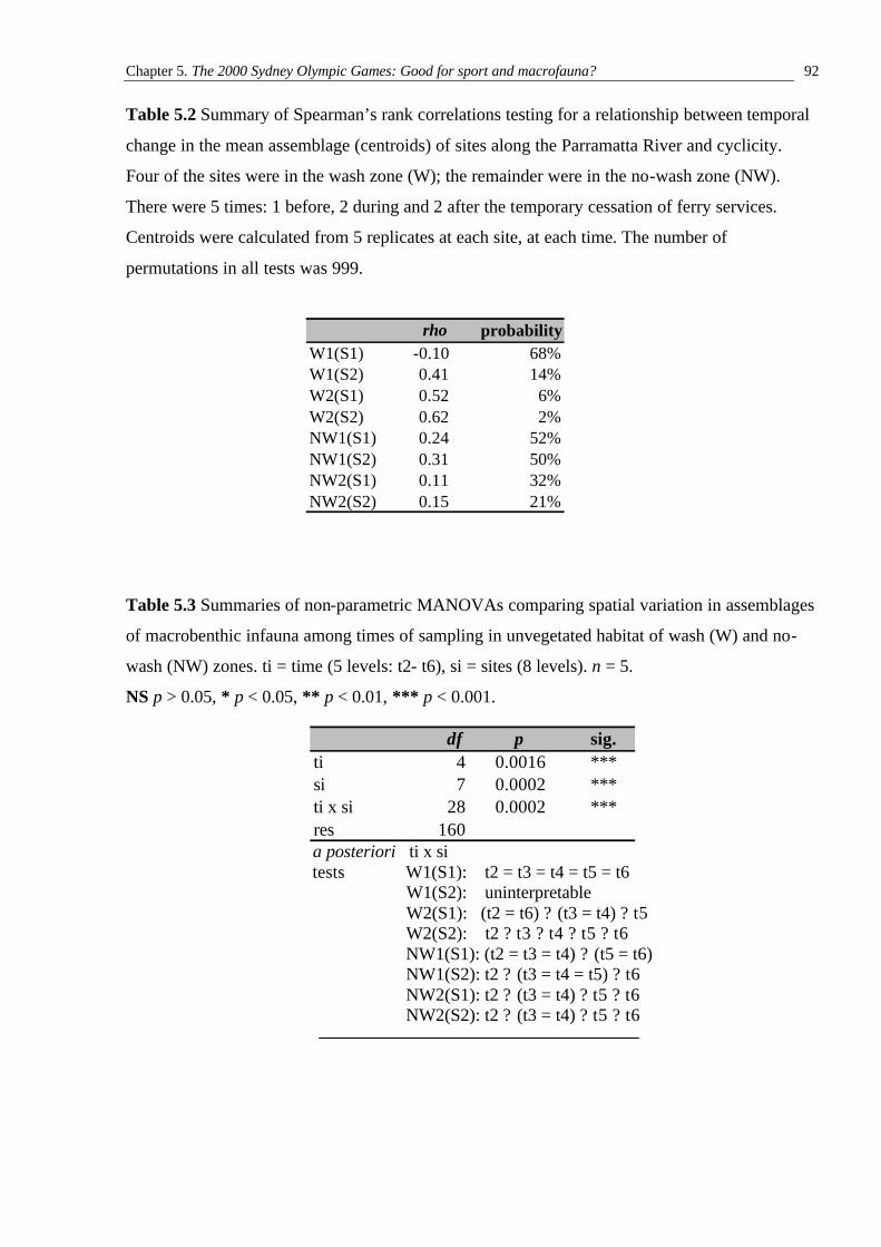
Chapter 5. The 2000 Sydney Olympic Games: Good for sport and macrofauna? 92
Table 5.2 Summary of Spearman’s rank correlations testing for a relationship between temporal
change in the mean assemblage (centroids) of sites along the Parramatta River and cyclicity.
Four of the sites were in the wash zone (W); the remainder were in the no-wash zone (NW).
There were 5 times: 1 before, 2 during and 2 after the temporary cessation of ferry services.
Centroids were calculated from 5 replicates at each site, at each time. The number of
permutations in all tests was 999.
Table 5.3 Summaries of non-parametric MANOVAs comparing spatial variation in assemblages
of macrobenthic infauna among times of sampling in unvegetated habitat of wash (W) and no-
wash (NW) zones. ti = time (5 levels: t2- t6), si = sites (8 levels). n = 5.
NS p > 0.05, * p < 0.05, ** p < 0.01, *** p < 0.001.
a posteriori ti x si tests W1(S1): t2 = t3 = t4 = t5 = t6 W1(S2): uninterpretable W2(S1): (t2 = t6) ? (t3 = t4) ? t5 W2(S2): t2 ? t3 ? t4 ? t5 ? t6 NW1(S1): (t2 = t3 = t4) ? (t5 = t6) NW1(S2): t2 ? (t3 = t4 = t5) ? t6 NW2(S1): t2 ? (t3 = t4) ? t5 ? t6 NW2(S2): t2 ? (t3 = t4) ? t5 ? t6
rho probabilityW1(S1) -0.10 68%W1(S2) 0.41 14%W2(S1) 0.52 6%W2(S2) 0.62 2%NW1(S1) 0.24 52%NW1(S2) 0.31 50%NW2(S1) 0.11 32%NW2(S2) 0.15 21%
df p sig.ti 4 0.0016 ***si 7 0.0002 ***ti x si 28 0.0002 ***res 160
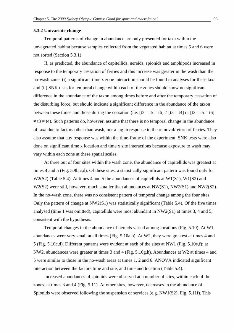
Chapter 5. The 2000 Sydney Olympic Games: Good for sport and macrofauna? 93
5.3.2 Univariate change
Temporal patterns of change in abundance are only presented for taxa within the
unvegetated habitat because samples collected from the vegetated habitat at times 5 and 6 were
not sorted (Section 5.3.1).
If, as predicted, the abundance of capitellids, nereids, spionids and amphipods increased in
response to the temporary cessation of ferries and this increase was greater in the wash than the
no-wash zone: (i) a significant time x zone interaction should be found in analyses for these taxa
and (ii) SNK tests for temporal change within each of the zones should show no significant
difference in the abundance of the taxon among times before and after the temporary cessation of
the disturbing force, but should indicate a significant difference in the abundance of the taxon
between these times and those during the cessation (i.e. [t2 = t5 = t6] ≠ [t3 = t4] or [t2 = t5 = t6]
≠ t3 ≠ t4). Such patterns do, however, assume that there is no temporal change in the abundance
of taxa due to factors other than wash, nor a lag in response to the removal/return of ferries. They
also assume that any response was within the time-frame of the experiment. SNK tests were also
done on significant time x location and time x site interactions because exposure to wash may
vary within each zone at these spatial scales.
At three out of four sites within the wash zone, the abundance of capitellids was greatest at
times 4 and 5 (Fig. 5.9b,c,d). Of these sites, a statistically significant pattern was found only for
W2(S2) (Table 5.4). At times 4 and 5 the abundances of capitellids at W1(S1), W1(S2) and
W2(S2) were still, however, much smaller than abundances at NW(S1), NW2(S1) and NW2(S2).
In the no-wash zone, there was no consistent pattern of temporal change among the four sites.
Only the pattern of change at NW2(S1) was statistically significant (Table 5.4). Of the five times
analysed (time 1 was omitted), capitellids were most abundant in NW2(S1) at times 3, 4 and 5,
consistent with the hypothesis.
Temporal changes in the abundance of nereids varied among locations (Fig. 5.10). At W1,
abundances were very small at all times (Fig. 5.10a,b). At W2, they were greatest at times 4 and
5 (Fig. 5.10c,d). Different patterns were evident at each of the sites at NW1 (Fig. 5.10e,f); at
NW2, abundances were greater at times 3 and 4 (Fig. 5.10g,h). Abundances at W2 at times 4 and
5 were similar to those in the no-wash areas at times 1, 2 and 6. ANOVA indicated significant
interaction between the factors time and site, and time and location (Table 5.4).
Increased abundances of spionids were observed at a number of sites, within each of the
zones, at times 3 and 4 (Fig. 5.11). At other sites, however, decreases in the abundance of
Spionids were observed following the suspension of services (e.g. NW1(S2), Fig. 5.11f). This
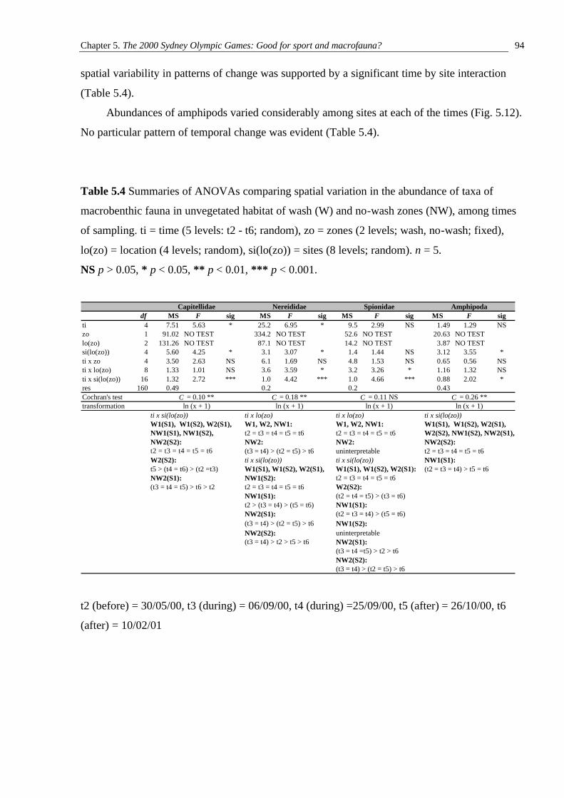
Chapter 5. The 2000 Sydney Olympic Games: Good for sport and macrofauna? 94
spatial variability in patterns of change was supported by a significant time by site interaction
(Table 5.4).
Abundances of amphipods varied considerably among sites at each of the times (Fig. 5.12).
No particular pattern of temporal change was evident (Table 5.4).
Table 5.4 Summaries of ANOVAs comparing spatial variation in the abundance of taxa of
macrobenthic fauna in unvegetated habitat of wash (W) and no-wash zones (NW), among times
of sampling. ti = time (5 levels: t2 - t6; random), zo = zones (2 levels; wash, no-wash; fixed),
lo(zo) = location (4 levels; random), si(lo(zo)) = sites (8 levels; random). n = 5.
NS p > 0.05, * p < 0.05, ** p < 0.01, *** p < 0.001.
t2 (before) = 30/05/00, t3 (during) = 06/09/00, t4 (during) =25/09/00, t5 (after) = 26/10/00, t6
(after) = 10/02/01
df MS F sig MS F sig MS F sig MS F sigti 4 7.51 5.63 * 25.2 6.95 * 9.5 2.99 NS 1.49 1.29 NSzo 1 91.02 NO TEST 334.2 NO TEST 52.6 NO TEST 20.63 NO TESTlo(zo) 2 131.26 NO TEST 87.1 NO TEST 14.2 NO TEST 3.87 NO TESTsi(lo(zo)) 4 5.60 4.25 * 3.1 3.07 * 1.4 1.44 NS 3.12 3.55 *ti x zo 4 3.50 2.63 NS 6.1 1.69 NS 4.8 1.53 NS 0.65 0.56 NSti x lo(zo) 8 1.33 1.01 NS 3.6 3.59 * 3.2 3.26 * 1.16 1.32 NSti x si(lo(zo)) 16 1.32 2.72 *** 1.0 4.42 *** 1.0 4.66 *** 0.88 2.02 *res 160 0.49 0.2 0.2 0.43Cochran's testtransformation
ti x si(lo(zo)) ti x lo(zo) ti x lo(zo) ti x si(lo(zo))W1(S1), W1(S2), W2(S1), W1, W2, NW1: W1, W2, NW1: W1(S1), W1(S2), W2(S1),NW1(S1), NW1(S2), t2 = t3 = t4 = t5 = t6 t2 = t3 = t4 = t5 = t6 W2(S2), NW1(S2), NW2(S1),NW2(S2): NW2: NW2: NW2(S2):t2 = t3 = t4 = t5 = t6 (t3 = t4) > (t2 = t5) > t6 uninterpretable t2 = t3 = t4 = t5 = t6W2(S2): ti x si(lo(zo)) ti x si(lo(zo)) NW1(S1):t5 > (t4 = t6) > (t2 =t3) W1(S1), W1(S2), W2(S1), W1(S1), W1(S2), W2(S1): (t2 = t3 = t4) > t5 = t6NW2(S1): NW1(S2): t2 = t3 = t4 = t5 = t6(t3 = t4 = t5) > t6 > t2 t2 = t3 = t4 = t5 = t6 W2(S2):
NW1(S1): (t2 = t4 = t5) > (t3 = t6)t2 > (t3 = t4) > (t5 = t6) NW1(S1):NW2(S1): (t2 = t3 = t4) > (t5 = t6)(t3 = t4) > (t2 = t5) > t6 NW1(S2):NW2(S2): uninterpretable(t3 = t4) > t2 > t5 > t6 NW2(S1):
(t3 = t4 =t5) > t2 > t6NW2(S2):(t3 = t4) > (t2 = t5) > t6
Amphipoda
C = 0.26 **ln (x + 1)
Nereididae
C = 0.18 **ln (x + 1)
Spionidae
C = 0.11 NSln (x + 1)
Capitellidae
C = 0.10 **ln (x + 1)
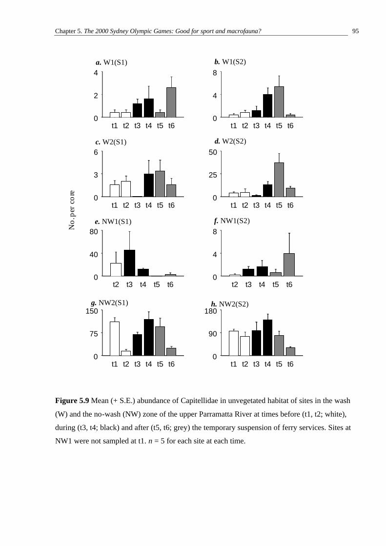
Chapter 5. The 2000 Sydney Olympic Games: Good for sport and macrofauna? 95
Figure 5.9 Mean (+ S.E.) abundance of Capitellidae in unvegetated habitat of sites in the wash
(W) and the no-wash (NW) zone of the upper Parramatta River at times before (t1, t2; white),
during (t3, t4; black) and after (t5, t6; grey) the temporary suspension of ferry services. Sites at
NW1 were not sampled at t1. n = 5 for each site at each time.
t1 t2 t3 t4 t5 t60
2
4
t1 t2 t3 t4 t5 t60
4
8
t1 t2 t3 t4 t5 t60
3
6
t1 t2 t3 t4 t5 t60
25
50
t2 t3 t4 t5 t60
40
80
t2 t3 t4 t5 t60
4
8
t1 t2 t3 t4 t5 t60
75
150g. NW2(S1)
t1 t2 t3 t4 t5 t60
90
180h. NW2(S2)
a. W1(S1) b. W1(S2)
c. W2(S1) d. W2(S2)
e. NW1(S1) f. NW1(S2)
No.
per
core
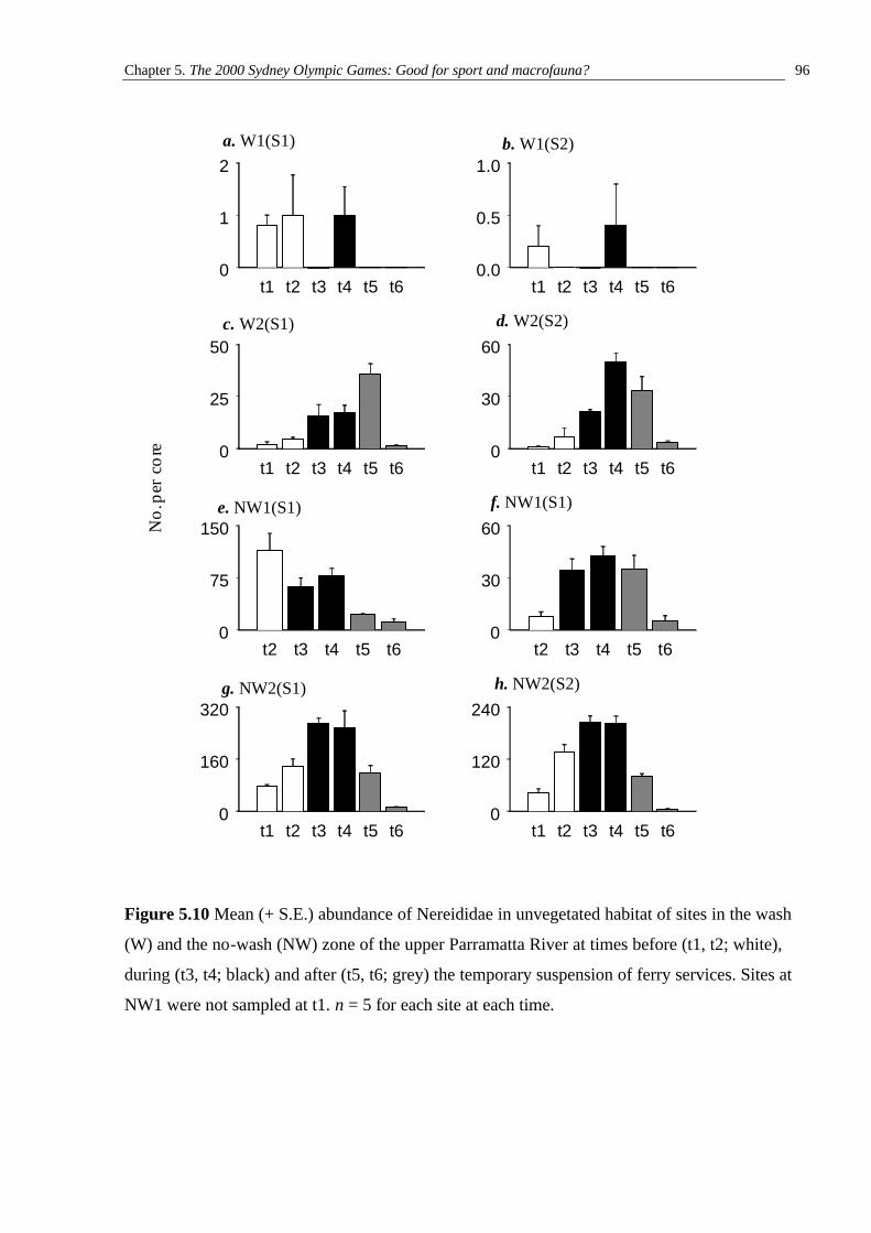
Chapter 5. The 2000 Sydney Olympic Games: Good for sport and macrofauna? 96
Figure 5.10 Mean (+ S.E.) abundance of Nereididae in unvegetated habitat of sites in the wash
(W) and the no-wash (NW) zone of the upper Parramatta River at times before (t1, t2; white),
during (t3, t4; black) and after (t5, t6; grey) the temporary suspension of ferry services. Sites at
NW1 were not sampled at t1. n = 5 for each site at each time.
t1 t2 t3 t4 t5 t60
1
2
t1 t2 t3 t4 t5 t60.0
0.5
1.0
t1 t2 t3 t4 t5 t60
25
50
t1 t2 t3 t4 t5 t60
30
60
d. W2(S2)
t2 t3 t4 t5 t60
75
150e. NW1(S1)
t2 t3 t4 t5 t60
30
60
t1 t2 t3 t4 t5 t60
160
320
t1 t2 t3 t4 t5 t60
120
240
a. W1(S1) b. W1(S2)
c. W2(S1)
f. NW1(S1)
g. NW2(S1) h. NW2(S2)
No.
per
core
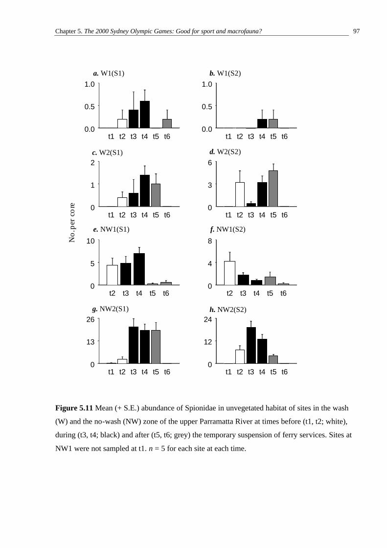
Chapter 5. The 2000 Sydney Olympic Games: Good for sport and macrofauna? 97
Figure 5.11 Mean (+ S.E.) abundance of Spionidae in unvegetated habitat of sites in the wash
(W) and the no-wash (NW) zone of the upper Parramatta River at times before (t1, t2; white),
during (t3, t4; black) and after (t5, t6; grey) the temporary suspension of ferry services. Sites at
NW1 were not sampled at t1. n = 5 for each site at each time.
t1 t2 t3 t4 t5 t60.0
0.5
1.0
t1 t2 t3 t4 t5 t60.0
0.5
1.0
t1 t2 t3 t4 t5 t60
1
2
t1 t2 t3 t4 t5 t60
3
6
t2 t3 t4 t5 t60
5
10
e. NW1(S1)
t2 t3 t4 t5 t60
4
8
f. NW1(S2)
t1 t2 t3 t4 t5 t60
13
26
t1 t2 t3 t4 t5 t60
12
24
a. W1(S1) b. W1(S2)
c. W2(S1) d. W2(S2)
g. NW2(S1) h. NW2(S2)
No.
per
core
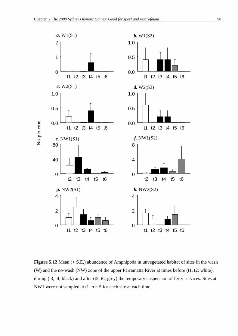
Chapter 5. The 2000 Sydney Olympic Games: Good for sport and macrofauna? 98
Figure 5.12 Mean (+ S.E.) abundance of Amphipoda in unvegetated habitat of sites in the wash
(W) and the no-wash (NW) zone of the upper Parramatta River at times before (t1, t2; white),
during (t3, t4; black) and after (t5, t6; grey) the temporary suspension of ferry services. Sites at
NW1 were not sampled at t1. n = 5 for each site at each time.
t1 t2 t3 t4 t5 t60
1
2
t1 t2 t3 t4 t5 t60.0
0.5
1.0
t1 t2 t3 t4 t5 t60.0
0.5
1.0
c. W2(S1)
t1 t2 t3 t4 t5 t60.0
0.5
1.0
t2 t3 t4 t5 t60
40
80e. NW1(S1)
t2 t3 t4 t5 t60
4
8
t1 t2 t3 t4 t5 t60
2
4
t1 t2 t3 t4 t5 t60
2
4
a. W1(S1) b. W1(S2)
d. W2(S2)
f. NW1(S2)
g. NW2(S1) h. NW2(S2)
No.
per
core
Chapter 5. The 2000 Sydney Olympic Games: Good for sport and macrofauna? 99
5.4 Discussion
In the unvegetated habitat, assemblages at the majority of sites within the wash zone
changed to become more similar to those of the no-wash zone following the temporary
suspension of RiverCat ferry services. Several months after the return of services, these
assemblages had returned to their previous, disturbed, state. Changes to the assemblages in some
sites of the no-wash zone were also observed, coincident with the temporary cessation. Changes
to the assemblages of the no-wash zone were, however, much smaller than changes to the
assemblages of the wash zone. Following the return of services, the assemblages of these sites in
the no-wash zone initially displayed change towards their previous state, before becoming very
different from the assemblages found at any of the other times.
In contrast, assemblages in neither the wash nor the no-wash zone of the vegetated habitat
appeared to respond to the temporary suspension of services. Assemblages changed little
between times of sampling and any change that did occur appeared random.
The greater change in the assemblages of the unvegetated habitat of the wash zone than the
no-wash zone following the suspension of ferry services is consistent with the removal of the
disturbance of wash. Had change been due to some other disturbance associated with ferries (e.g.
the emission of fuel or exhaust), a similar pattern of change should have been observed between
the two zones following the cessation of services because the number of ferries traveling along
these sections of river was identical. Thus, the pattern of change supports the model that wash is
responsible for differences in the assemblages of wash and no-wash zones.
Change to assemblages of the unvegetated habitat appeared to be caused by changes in the
abundances of capitellids and nereids. Abundances of these taxa increased following the
suspension of services and decreased following their re-introduction. Changes in the abundances
of capitellids and nereids and the structure of assemblages did, however, lag behind changes to
ferry services. In most sites, no changes to assemblages or the abundances of capitellids and
nereids were evident a week after the stoppage. It was generally not until a month after the
stoppage that a change was seen. This is not surprising considering that colonization will only be
observed if: (i) settlement occurs and (ii) organisms reach a size greater than 500 µm in
diameter, such that they are retained on the sieve. Previous studies have suggested it may take
over 6 months for abundances to peak (Pearson and Rosenberg, 1978; Lu and Wu, 2000).
A lag was also seen between the re-introduction of services and the return of
assemblages/abundances to a disturbed state. This suggests that patterns in assemblages and
abundances of taxa, between wash and no-wash zones, are not due to greater rates of erosion of
organisms in the wash zone. Erosion of macrofauna is correlated with the velocity of wind and
Chapter 5. The 2000 Sydney Olympic Games: Good for sport and macrofauna? 100
the flux of sediment (Miller and Sternberg, 1988; Emerson and Grant, 1991; Armonies, 1992)
and can have a significant influence on patterns of distribution and abundance (e.g. Thrush,
1986; Frid, 1989; Emerson and Grant, 1991; Günther, 1992; Snelgrove et al., 1993). If erosion of
organisms were greater in the wash than in the no-wash zone, assemblages and abundances of
macrofauna in the wash zone should have reverted to a disturbed state immediately after the re-
introduction of ferry services. This was not the case and suggests that patterns in macrofauna are
an indirect effect of wash.
Sediment-related variables are widely believed to be important in structuring infaunal
assemblages (reviewed by Gray, 1974, 1981; Rhoads, 1974; Probert, 1984, but see Zajac and
Whitlatch, 1982a,b). The distributions of infaunal species are closely correlated with certain
types of sediment (e.g. Rhoads, 1974; Scheltema, 1974; Butman, 1987; Snelgrove and Butman,
1994) and several studies have found a strong relationship between the distributions of animals
and organic matter, a dominant source of food for deposit-feeders (Longbottom, 1970; Field,
1971; Ishikawa, 1989). Properties of the sediment, such as grain-size and organic content, are not
only determined by the availability materials but also by the amount of energy imparted to the
sediment from hydrodynamic processes (summarized in Royse, 1970). If: (i) properties of the
sediment are important in determining the structure of assemblages and (ii) waves alter these
properties in the wash zone, assemblages would differ between the wash zone and the no-wash
zone due to an indirect effect of wash.
Changes in the abundance of capitellids and nereids were generally greater in the no-wash
than in the wash zone. A possible model to explain this pattern is that the availability of larvae
was greater in the no-wash than in the wash zone and may have limited colonization in the latter
area. This is contrary to the model that exposure to boat-generated waves increases larval fluxes
over intertidal mudflats (see Bertness et al., 1991; Gaines and Bertness, 1993). If this were the
case, settlement would be less in the no-wash zone.
In both the wash and no-wash zones, within-site variability in assemblages was smallest at
times 4 and 5 (i.e. during the cessation and immediately after the return of ferries). This supports
the model that the disturbance of wash increases spatial variability in assemblages. If this were
the case, the pattern, described in Chapter 4 (of greater within-site variability in the wash than
the no-wash zone) may be attributed to the different intensities of the disturbance between these
places.
In any case, the results of this study must be treated with caution since neither undisturbed
locations nor locations where ferries continued to run were used in analyses to control for
background temporal and spatial variation in assemblages. The control locations sampled in this
Chapter 5. The 2000 Sydney Olympic Games: Good for sport and macrofauna? 101
study were situated more than four kilometres downstream from the wash and no wash zones,
along a much wider section of river. They are likely to have been more exposed to wind-
generated waves, subject to greater volumes of recreational boat-traffic and have had a greater
salinity than were the case in sites further upstream. The assemblages in control locations were
significantly different from those in wash or no-wash zones. They were consequently omitted
from analyses because background temporal and spatial variability in these is unlikely to have
been representative of change in the wash or no-wash zones.
This problem could not be avoided given that: (i) ferries only continued to operate to the
west of Homebush Bay (Fig. 5.1) and (ii) there was a paucity of suitable habitat for sampling
immediately downstream of the Homebush Bay ferry wharf. This problem of inappropriate
control locations is a common one given the lack of randomization of unplanned impacts (Wiens
and Parker, 1995). When inappropriate controls are included in analyses, they frequently lead to
confounding of results.
In interpreting the results of this study, it was therefore assumed that background temporal
variability in assemblages was negligible. Given that this study ran over a period of 10 months
this assumption is probably not justified. Biological systems are not static and unchanging -
many taxa display seasonal changes in abundance that reflect patterns of larval reproduction and
transport (e.g. Lively et al., 1993; Turner et al., 1995). Therefore, the failure of assemblages in
many sites to return to their previous state (i.e. composition prior to the temporary stoppage) by
time 6 does not necessarily mean that no recovery occurred (see discussion of endpoints in
Grayson et al., 1999).
The impossibility of determining whether there was any temporal change to assemblages of
the upper Parramatta River that was a result of factors other than the stoppage/return of ferries
was particularly problematic in the case of assemblages in the unvegeted habitat of the no-wash
zone. Following the return of services, these assemblages did not appear to return to their
previous, presumably impacted, state. They appeared to be strongly influenced by some other
factor between sampling times 5 and 6.
This is not the first study to observe a change in the ecology of benthic organisms
following the cessation of ferry services. Davidson (1996, 1997) observed an increase in the
abundance of molluscs on intertidal boulders in the Tory Channel and Queen Charlotte Sound,
New Zealand, coincident with the off-seasons of the fast ferry, Condor 10. Although sampling
was confounded with season, such change was not observed in control sites sheltered from wash,
suggesting that the ferries were responsible for the pattern. These results suggest that the
ecological impacts of wash are reversible.
Chapter 5. The 2000 Sydney Olympic Games: Good for sport and macrofauna? 102
In the present study, the abundances of capitellid and nereid polychaetes increased in the
wash zone and in some sites of the no-wash zone during the temporary cessation of RiverCat
ferry services. Abundances decreased following the return of services. Depressed abundances
during the operation of services may be due to a greater rate of mortality of organisms, decreased
rates of settlement or the erosion and passive transport of organisms down-stream. Davidson
(1996, 1997) found increased numbers of recently dead and dying organisms in fixed quadrats
during the operation of the Condor 10 than during the off-season. Thus, ferry services appeared
to be responsible for increased mortality of subtidal organisms in the Tory Channel. Here, the
return of assemblages to a similar state as found prior to the disturbance took several months. If
changes were due to mortality, one would not expect such a long lag between the return of
ferries and change in the assemblages.
In this study, the lack of response to the suspension of services by assemblages in the
vegetated habitat may have been due to several factors. First, wash may not be important in
determining the structure of assemblages in this habitat. This would be the case if
pneumatophores dissipate wave-energy and/or the roots below-ground stabilize sediment such
that invertebrates living in this habitat do not ‘feel’ the effects of wash. This model was,
however, not supported by the results in Chapter 4. It could also be the case if the types of
animal found in this habitat were resistant to the effects of wash. Given that the types of
invertebrate present in this habitat were similar to those in the unvegetated sediment, where there
appeared to be an impact of wash, this is also unlikely.
The second model is that wash is important in structuring the faunal assemblages of
vegetated habitats, but change was not seen following the cessation of services because
insufficient time was allowed for this to occur. Benthic ‘recovery’ following a disturbance is
generally considered to be a slow process that may take up to several years (e.g. Boesch and
Rosenberg, 1981; Stachowitsch, 1991; Lu and Wu, 2000). While change was observed in the
unvegetated habitat over the period of this study, longer periods may be required in vegetated
habitats. Empirical studies and modelling suggest that the interaction of tidal currents and
vegetation generates zones of stagnant water in mangrove forests (Furukawa et al., 1997;
Wolanski and Ridd, 1986). This may increase the time required for recolonization of sediment
because settlement is dependent on the availability of larvae in the water-column (e.g. Zajac and
Whitlatch, 1982a; Kalejta and Hockey, 1991).
Finally, change in the assemblages of vegetated habitat may not have occurred following
the removal of the disturbing force because the habitat was irreversibly modified by the
Chapter 5. The 2000 Sydney Olympic Games: Good for sport and macrofauna? 103
disturbance, such that it was no longer able to support the great densities of taxa found in the no-
wash zone.
Thus, while the results presented here suggest that wash is important in structuring the
assemblages of unvegetated but not vegetated habitat, further manipulative experiments would
enable the results to be interpreted with greater confidence.
CHAPTER 6
MORE EXPERIMENTS TO DETERMINE THE ROLE OF RIVERCAT WASH IN STRUCTURING ASSEMBLAGES OF MACROBENTHIC INFAUNA
6.1 Introduction
A central issue in the assessment of environmental impacts is the distinction of change to
assemblages induced by anthropogenic disturbance, from variation in those assemblages due to
natural spatial and temporal variability (Levin, 1992; Peterson, 1993; Osenberg et al., 1994).
Where an environmental impact is large relative to background variation, this is relatively simple
(Green, 1979). In soft-sediment habitats, benthic organisms are, however, often patchy in
distribution and change markedly over short time-periods (Barry and Dayton, 1991; McIntosh,
1991; Morrisey et al., 1992). This makes the detection of putative impacts very difficult.
Statistical tests may not support an ecological impact despite differences in assemblages between
control and impact locations.
Physical factors, such as depth and movement of water and sediment-type (e.g. Thorson,
1957; Gray, 1974; Barry and Dayton, 1991) are thought to be most important in determining
large-scale patterns of distribution of benthic infauna. Disturbances, biotic and/or abiotic factors
maintain heterogeneity at smaller scales (< 100s metres; Thrush et al., 1989; Barry and Dayton,
1991). The role of sediment-related variables in structuring infaunal assemblages has received
particular attention (reviewed by Rhoads, 1974; Gray, 1974, 1981; Probert, 1984). The
distributions of infaunal species are closely correlated with certain types of sediment (e.g.
Rhoads, 1974; Scheltema, 1974; Butman, 1987; Snelgrove and Butman, 1994). Contour, grain-
size, porosity, organic content and adsorbed chemicals are believed to be important in
determining recruitment of polychaetes and crustaceans (Jones, 1950; Thorson, 1957; Rhoads
and Young, 1970; Gray, 1974).
Little experimental work has, however, been done to test the effects of sediment on the
recolonization and succession of defaunated sediment (but see Zajac and Whitlatch, 1982a,
1982b; Stark, 1996; Wu and Shin, 1997). Zajac and Whitlatch (1982a, 1982b) showed that there
were few differences in the initial colonization of defaunated plots of mud and sand. Wu and
Shin (1997) showed that characteristics of the sediment were only significant for colonization of
gastropods and bivalves, but not for polychaetes and amphipods.
In Chapter 4, assemblages of macrobenthic infauna differed between wash and no-wash
zones of the upper Parramatta River, in vegetated and unvegetated habitat, at two times of
sampling. These differences were, however, not statistically significant, possibly due to
Chapter 6. The role of RiverCat wash in structuring assemblages of macrobenthic infauna 105
considerable variability in assemblages at the scales of replicates (metres), sites (10s of metres)
and locations (100s of metres) within zones. While sorting these samples, it was observed that
characteristics of the sediment, such as grain-size and organic content also varied over similar
spatial scales. This variability appeared particularly large from site to site. If characteristics of
the sediment are important in determining the distribution and abundance of taxa along the
Parramatta River, large spatial variability in characteristics of the sediment may be one important
factor contributing to large natural variability in the distribution and abundance of infauna.
Artificial habitats, which offer the same microhabitat across different sites (e.g. Rosenberg
and Resh, 1982; Edgar, 1991; Cairns and Pratt, 1993; Bologna and Heck, 1999), can be used to
reduce natural variability in assemblages so that the effects of differing levels of a factor of
interest might be more easily determined. While many studies, such as those employing acrylic
plates (e.g. Deutsch, 1980) or artificial seagrass units (e.g. Barber et al., 1979), have used this
strategy to sample organisms associated with hard substrata, few have adopted this approach for
soft sediments. If different sediments do determine the structure of infaunal assemblages, the use
of artificial sampling units containing homogeneous sediment should reduce variability in
assemblages among replicates and sites, allowing ecological impacts to be measured more easily.
It was hypothesised that if homogeneous sediment was transplanted to various sites along the
Parramatta River, the assemblages that accumulate in this sediment over a period of 1 month
would be less variable among replicates and sites than those that accumulate in natural sediment.
The sediment was defaunated because the recruitment of macro-invertebrates may be affected by
the fauna already living in the sediment (e.g. Highsmith, 1982; Pawlik, 1986) and similar
conditions were required in all replicates. It was also hypothesised that, if spatial variability was
smaller in the homogeneous sediment than in the site-specific sediment, a stronger pattern
between wash and no-wash zones would be seen. This hypothesis does, however, assume a direct
effect of wash on colonization. If the effect of wash on colonization is indirect, this pattern will
not be seen.
Properties of the sediment, such as grain-size are not only a function of the sizes of available
materials, but are also determined by the amount of energy imparted to the sediment from
hydrodynamic processes (summarized in Royse, 1970). If: (i) properties of the sediment are
important in determining colonization and (ii) waves alter these properties in the wash zone,
colonization would differ between the wash zone and the no-wash zone due to an indirect effect
of wash. In this case, colonization of homogeneous sediment would not differ between the wash
and the no-wash zone. Differences in assemblages between the two zones would, instead, be
greater in the site-specific than the homogeneous sediment.
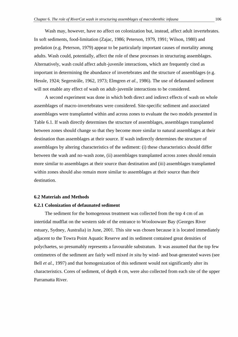
Chapter 6. The role of RiverCat wash in structuring assemblages of macrobenthic infauna 106
Wash may, however, have no affect on colonization but, instead, affect adult invertebrates.
In soft sediments, food-limitation (Zajac, 1986; Peterson, 1979, 1991; Wilson, 1980) and
predation (e.g. Peterson, 1979) appear to be particularly important causes of mortality among
adults. Wash could, potentially, affect the role of these processes in structuring assemblages.
Alternatively, wash could affect adult-juvenile interactions, which are frequently cited as
important in determining the abundance of invertebrates and the structure of assemblages (e.g.
Hessle, 1924; Segerstråle, 1962, 1973; Elmgren et al., 1986). The use of defaunated sediment
will not enable any effect of wash on adult-juvenile interactions to be considered.
A second experiment was done in which both direct and indirect effects of wash on whole
assemblages of macro-invertebrates were considered. Site-specific sediment and associated
assemblages were transplanted within and across zones to evaluate the two models presented in
Table 6.1. If wash directly determines the structure of assemblages, assemblages transplanted
between zones should change so that they become more similar to natural assemblages at their
destination than assemblages at their source. If wash indirectly determines the structure of
assemblages by altering characteristics of the sediment: (i) these characteristics should differ
between the wash and no-wash zone, (ii) assemblages transplanted across zones should remain
more similar to assemblages at their source than destination and (iii) assemblages transplanted
within zones should also remain more similar to assemblages at their source than their
destination.
6.2 Materials and Methods
6.2.1 Colonization of defaunated sediment
The sediment for the homogenous treatment was collected from the top 4 cm of an
intertidal mudflat on the western side of the entrance to Woolooware Bay (Georges River
estuary, Sydney, Australia) in June, 2001. This site was chosen because it is located immediately
adjacent to the Towra Point Aquatic Reserve and its sediment contained great densities of
polychaetes, so presumably represents a favourable substratum. It was assumed that the top few
centimetres of the sediment are fairly well mixed in situ by wind- and boat-generated waves (see
Bell et al., 1997) and that homogenization of this sediment would not significantly alter its
characteristics. Cores of sediment, of depth 4 cm, were also collected from each site of the upper
Parramatta River.
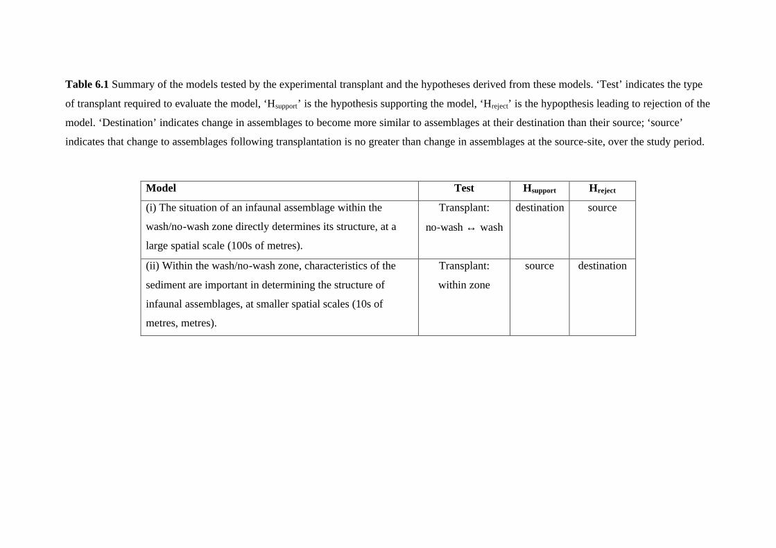
Table 6.1 Summary of the models tested by the experimental transplant and the hypotheses derived from these models. ‘Test’ indicates the type
of transplant required to evaluate the model, ‘Hsupport’ is the hypothesis supporting the model, ‘Hreject’ is the hypopthesis leading to rejection of the
model. ‘Destination’ indicates change in assemblages to become more similar to assemblages at their destination than their source; ‘source’
indicates that change to assemblages following transplantation is no greater than change in assemblages at the source-site, over the study period.
Model Test Hsupport Hreject
(i) The situation of an infaunal assemblage within the
wash/no-wash zone directly determines its structure, at a
large spatial scale (100s of metres).
Transplant:
no-wash ↔ wash
destination source
(ii) Within the wash/no-wash zone, characteristics of the
sediment are important in determining the structure of
infaunal assemblages, at smaller spatial scales (10s of
metres, metres).
Transplant:
within zone
source destination
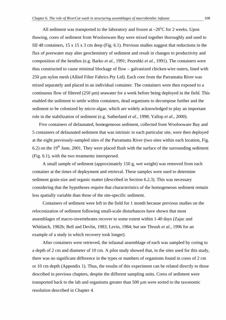
Chapter 6. The role of RiverCat wash in structuring assemblages of macrobenthic infauna 108
All sediment was transported to the laboratory and frozen at –20oC for 2 weeks. Upon
thawing, cores of sediment from Woolooware Bay were mixed together thoroughly and used to
fill 48 containers, 15 x 15 x 3 cm deep (Fig. 6.1). Previous studies suggest that reductions in the
flux of porewater may alter geochemistry of sediment and result in changes to productivity and
composition of the benthos (e.g. Barko et al., 1991; Pezeshki et al., 1991). The containers were
thus constructed to cause minimal blockage of flow – galvanized chicken-wire outers, lined with
250 µm nylon mesh (Allied Filter Fabrics Pty Ltd). Each core from the Parramatta River was
mixed separately and placed in an individual container. The containers were then exposed to a
continuous flow of filtered (250 µm) seawater for a week before being deployed in the field. This
enabled the sediment to settle within containers, dead organisms to decompose further and the
sediment to be colonized by micro-algae, which are widely acknowledged to play an important
role in the stabilization of sediment (e.g. Sutherland et al., 1998; Yallop et al., 2000).
Five containers of defaunated, homogeneous sediment, collected from Woolooware Bay and
5 containers of defaunated sediment that was intrinsic to each particular site, were then deployed
at the eight previously-sampled sites of the Parramatta River (two sites within each location, Fig.
6.2) on the 19th June, 2001. They were placed flush with the surface of the surrounding sediment
(Fig. 6.1), with the two treatments interspersed.
A small sample of sediment (approximately 150 g, wet weight) was removed from each
container at the times of deployment and retrieval. These samples were used to determine
sediment grain-size and organic matter (described in Section 6.2.3). This was necessary
considering that the hypotheses require that characteristics of the homogeneous sediment remain
less spatially variable than those of the site-specific sediment.
Containers of sediment were left in the field for 1 month because previous studies on the
reloconization of sediment following small-scale disturbances have shown that most
assemblages of macro-invertebrates recover to some extent within 1-40 days (Zajac and
Whitlatch, 1982b; Bell and Devlin, 1983; Levin, 1984; but see Thrush et al., 1996 for an
example of a study in which recovery took longer).
After containers were retrieved, the infaunal assemblage of each was sampled by coring to
a depth of 2 cm and diameter of 10 cm. A pilot study showed that, in the sites used for this study,
there was no significant difference in the types or numbers of organisms found in cores of 2 cm
or 10 cm depth (Appendix 1). Thus, the results of this experiment can be related directly to those
described in previous chapters, despite the different sampling units. Cores of sediment were
transported back to the lab and organisms greater than 500 µm were sorted to the taxonomic
resolution described in Chapter 4.
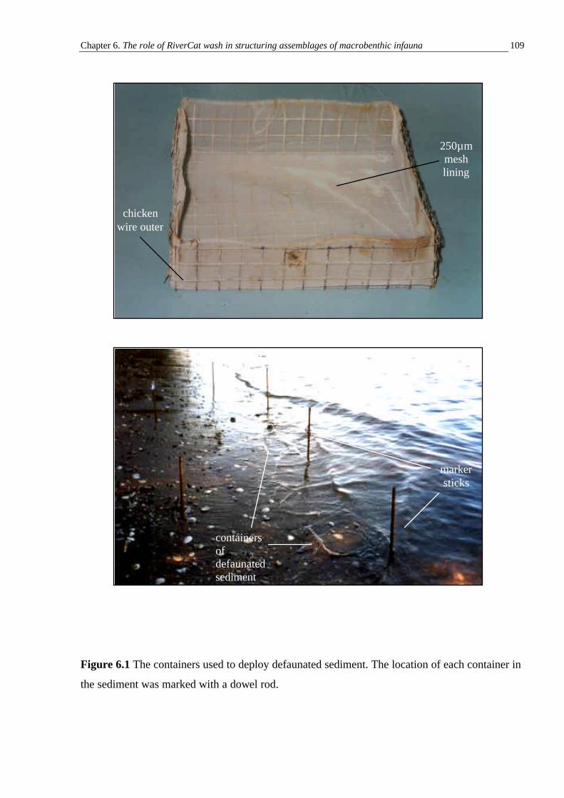
Chapter 6. The role of RiverCat wash in structuring assemblages of macrobenthic infauna 109
Figure 6.1 The containers used to deploy defaunated sediment. The location of each container in
the sediment was marked with a dowel rod.
250µm mesh lining
chicken wire outer
marker sticks
containers of defaunated sediment
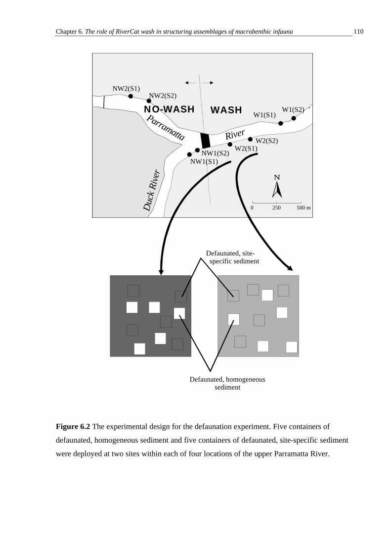
Chapter 6. The role of RiverCat wash in structuring assemblages of macrobenthic infauna 110
Figure 6.2 The experimental design for the defaunation experiment. Five containers of
defaunated, homogeneous sediment and five containers of defaunated, site-specific sediment
were deployed at two sites within each of four locations of the upper Parramatta River.
Duc
k Ri
ver
Parramatta River
NO-WASH WASH
W2(S1)W2(S2)
W1(S1)W1(S2)
NW1(S1)NW1(S2)
NW2(S1)NW2(S2)
0 250 500 m
Defaunated, homogeneous sediment
Defaunated, site- specific sediment
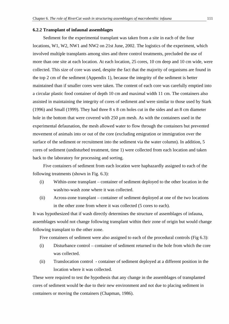
Chapter 6. The role of RiverCat wash in structuring assemblages of macrobenthic infauna 111
6.2.2 Transplant of infaunal assemblages
Sediment for the experimental transplant was taken from a site in each of the four
locations, W1, W2, NW1 and NW2 on 21st June, 2002. The logistics of the experiment, which
involved multiple transplants among sites and three control treatments, precluded the use of
more than one site at each location. At each location, 25 cores, 10 cm deep and 10 cm wide, were
collected. This size of core was used, despite the fact that the majority of organisms are found in
the top 2 cm of the sediment (Appendix 1), because the integrity of the sediment is better
maintained than if smaller cores were taken. The content of each core was carefully emptied into
a circular plastic food container of depth 10 cm and maximal width 11 cm. The containers also
assisted in maintaining the integrity of cores of sediment and were similar to those used by Stark
(1996) and Small (1999). They had three 8 x 8 cm holes cut in the sides and an 8 cm diameter
hole in the bottom that were covered with 250 µm mesh. As with the containers used in the
experimental defaunation, the mesh allowed water to flow through the containers but prevented
movement of animals into or out of the core (excluding emigration or immigration over the
surface of the sediment or recruitment into the sediment via the water column). In addition, 5
cores of sediment (undisturbed treatment, time 1) were collected from each location and taken
back to the laboratory for processing and sorting.
Five containers of sediment from each location were haphazardly assigned to each of the
following treatments (shown in Fig. 6.3):
(i) Within-zone transplant – container of sediment deployed to the other location in the
wash/no-wash zone where it was collected.
(ii) Across-zone transplant – container of sediment deployed at one of the two locations
in the other zone from where it was collected (5 cores to each).
It was hypothesized that if wash directly determines the structure of assemblages of infauna,
assemblages would not change following transplant within their zone of origin but would change
following transplant to the other zone.
Five containers of sediment were also assigned to each of the procedural controls (Fig 6.3):
(i) Disturbance control – container of sediment returned to the hole from which the core
was collected.
(ii) Translocation control - container of sediment deployed at a different position in the
location where it was collected.
These were required to test the hypothesis that any change in the assemblages of transplanted
cores of sediment would be due to their new environment and not due to placing sediment in
containers or moving the containers (Chapman, 1986).
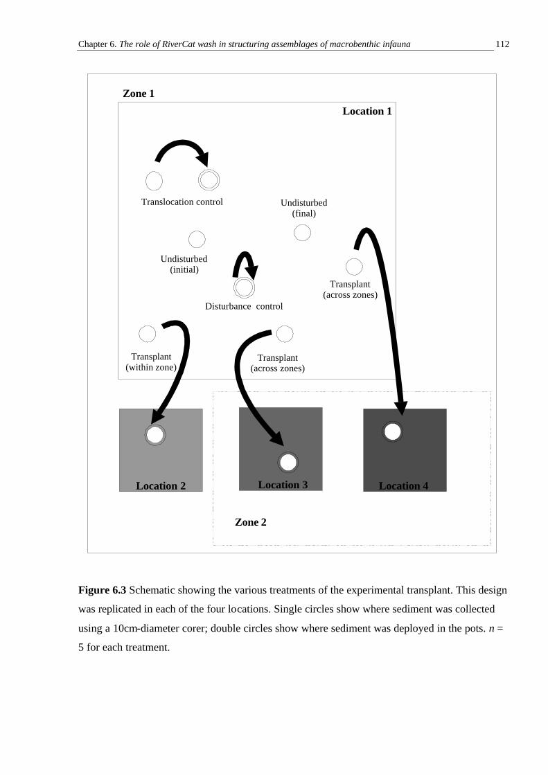
Chapter 6. The role of RiverCat wash in structuring assemblages of macrobenthic infauna 112
Figure 6.3 Schematic showing the various treatments of the experimental transplant. This design
was replicated in each of the four locations. Single circles show where sediment was collected
using a 10cm-diameter corer; double circles show where sediment was deployed in the pots. n =
5 for each treatment.
Translocation control
Disturbance control
Zone 1
Zone 2
Transplant(within zone)
Transplant(across zones)
Transplant(across zones)
Undisturbed(initial)
Undisturbed(final)
Location 3 Location 4
Location 1
Location 2
Chapter 6. The role of RiverCat wash in structuring assemblages of macrobenthic infauna 113
Containers were deployed by placing them in the holes left by the removal of cores of
sediment. They were left in the field for 6 weeks, following which they were retrieved and their
contents emptied into plastic bags. Samples were transported to the lab and organisms greater
than 500 µm were sorted to the taxonomic resolution previously described. A further 5 cores of
sediment were collected from each location to determine the structure of assemblages of
undisturbed sediment at the end of the experiment (undisturbed treatment, time 2).
Assemblages in the disturbance controls were compared to those in undisturbed sediment,
collected at time 2, to determine whether handling the sediment and deploying it in containers
had an effect on organisms. To determine whether movement of cores and translocation to a new
position in a location affected assemblages, assemblages of translocation controls were also
compared to those in undisturbed sediment, collected at time 2.
6.2.3 Analysis of sediment-related variables
The organic matter in samples was determined using a similar method to Dean (1974). A
teaspoon of sediment from each sample was placed in a pre-weighed crucible, dried to constant
weight at 70oC and then reweighed to give the dry weight of the sediment. The sediment was
then ashed at 480oC for 12 hours (see Byers et al., 1978). The amount of organic matter in each
sample was determined by weight-loss after combustion and is expressed as a percentage of total
dry weight.
The remaining sediment was used for the analysis of grain-size. Particles of diameter less
than 63 µm (4 Φ) were removed from the samples by repeatedly mixing the sample in 1 litre of
freshwater, leaving this to settle for a few minutes and then filtering the supernatant through pre-
weighed, grade 595/2 folded filter paper (Schleicher and Schuell, Germany). This was repeated
until the supernatant was clear. The filter papers and contents were dried to constant weight at
70oC and the weight of sediment determined. Excess water was decanted off the residual,
unsuspended sediment and this fraction was also dried to constant weight at 70oC. Once dried,
each sample of the coarser sediment was emptied into a column of dry sieves of mesh sizes 0, 1,
2, 2.5, 3, 3.5 and 4 Φ. The samples were sieved for 10 min using a Ro-Tap mechanical shaker
and the fraction retained on each sieve weighed separately. The proportion (by weight) of each
was calculated from the total weight.
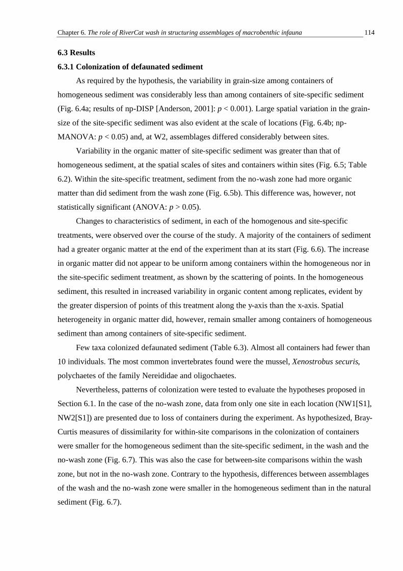
Chapter 6. The role of RiverCat wash in structuring assemblages of macrobenthic infauna 114
6.3 Results
6.3.1 Colonization of defaunated sediment
As required by the hypothesis, the variability in grain-size among containers of
homogeneous sediment was considerably less than among containers of site-specific sediment
(Fig. 6.4a; results of np-DISP [Anderson, 2001]: p < 0.001). Large spatial variation in the grain-
size of the site-specific sediment was also evident at the scale of locations (Fig. 6.4b; np-
MANOVA: p < 0.05) and, at W2, assemblages differed considerably between sites.
Variability in the organic matter of site-specific sediment was greater than that of
homogeneous sediment, at the spatial scales of sites and containers within sites (Fig. 6.5; Table
6.2). Within the site-specific treatment, sediment from the no-wash zone had more organic
matter than did sediment from the wash zone (Fig. 6.5b). This difference was, however, not
statistically significant (ANOVA: p > 0.05).
Changes to characteristics of sediment, in each of the homogenous and site-specific
treatments, were observed over the course of the study. A majority of the containers of sediment
had a greater organic matter at the end of the experiment than at its start (Fig. 6.6). The increase
in organic matter did not appear to be uniform among containers within the homogeneous nor in
the site-specific sediment treatment, as shown by the scattering of points. In the homogeneous
sediment, this resulted in increased variability in organic content among replicates, evident by
the greater dispersion of points of this treatment along the y-axis than the x-axis. Spatial
heterogeneity in organic matter did, however, remain smaller among containers of homogeneous
sediment than among containers of site-specific sediment.
Few taxa colonized defaunated sediment (Table 6.3). Almost all containers had fewer than
10 individuals. The most common invertebrates found were the mussel, Xenostrobus securis,
polychaetes of the family Nereididae and oligochaetes.
Nevertheless, patterns of colonization were tested to evaluate the hypotheses proposed in
Section 6.1. In the case of the no-wash zone, data from only one site in each location (NW1[S1],
NW2[S1]) are presented due to loss of containers during the experiment. As hypothesized, Bray-
Curtis measures of dissimilarity for within-site comparisons in the colonization of containers
were smaller for the homogeneous sediment than the site-specific sediment, in the wash and the
no-wash zone (Fig. 6.7). This was also the case for between-site comparisons within the wash
zone, but not in the no-wash zone. Contrary to the hypothesis, differences between assemblages
of the wash and the no-wash zone were smaller in the homogeneous sediment than in the natural
sediment (Fig. 6.7).
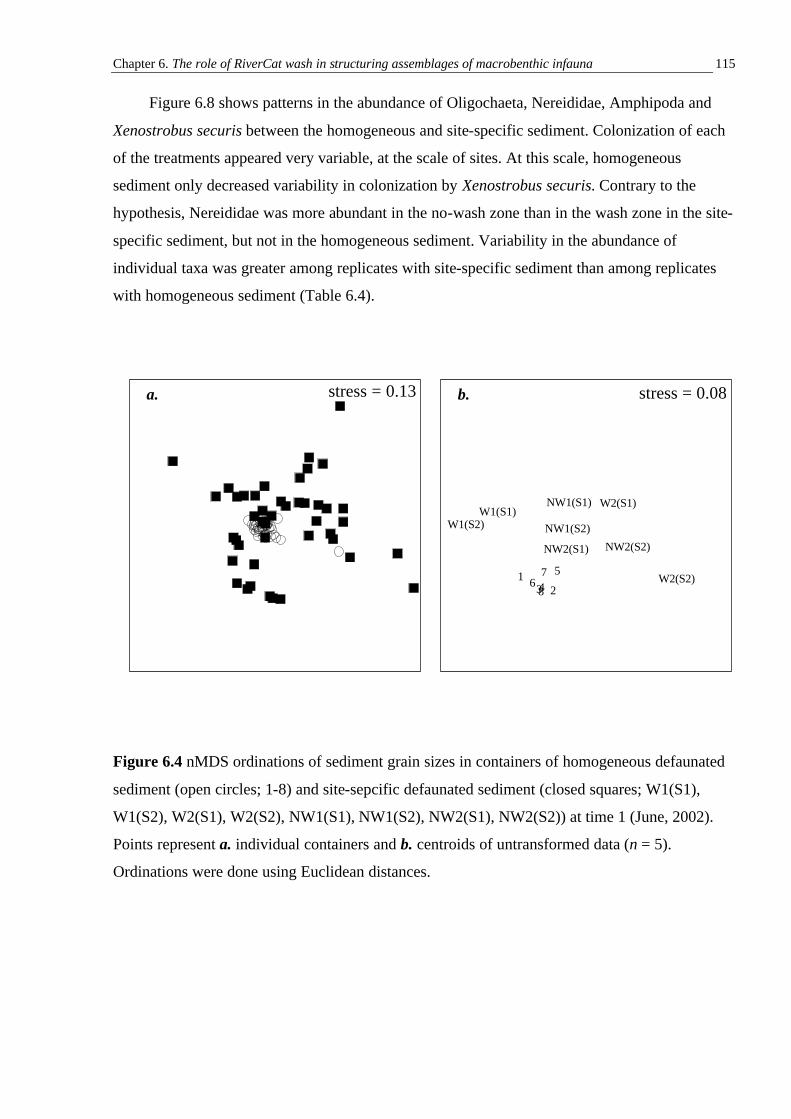
Chapter 6. The role of RiverCat wash in structuring assemblages of macrobenthic infauna 115
Figure 6.8 shows patterns in the abundance of Oligochaeta, Nereididae, Amphipoda and
Xenostrobus securis between the homogeneous and site-specific sediment. Colonization of each
of the treatments appeared very variable, at the scale of sites. At this scale, homogeneous
sediment only decreased variability in colonization by Xenostrobus securis. Contrary to the
hypothesis, Nereididae was more abundant in the no-wash zone than in the wash zone in the site-
specific sediment, but not in the homogeneous sediment. Variability in the abundance of
individual taxa was greater among replicates with site-specific sediment than among replicates
with homogeneous sediment (Table 6.4).
Figure 6.4 nMDS ordinations of sediment grain sizes in containers of homogeneous defaunated
sediment (open circles; 1-8) and site-sepcific defaunated sediment (closed squares; W1(S1),
W1(S2), W2(S1), W2(S2), NW1(S1), NW1(S2), NW2(S1), NW2(S2)) at time 1 (June, 2002).
Points represent a. individual containers and b. centroids of untransformed data (n = 5).
Ordinations were done using Euclidean distances.
stress = 0.13a. b.
12345
67
8
W1(S1)W1(S2)
W2(S1)
W2(S2)
NW1(S1)
NW1(S2)
NW2(S1) NW2(S2)
stress = 0.08
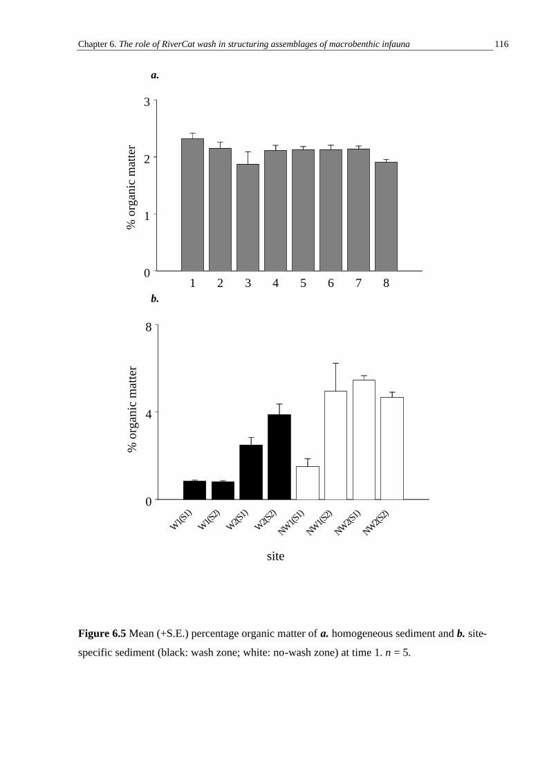
Chapter 6. The role of RiverCat wash in structuring assemblages of macrobenthic infauna 116
Figure 6.5 Mean (+S.E.) percentage organic matter of a. homogeneous sediment and b. site-
specific sediment (black: wash zone; white: no-wash zone) at time 1. n = 5.
1 2 3 4 5 6 7 80
1
2
3
% o
rgan
ic m
atte
r
W1(S
1)
W1(S
2)
W2(S
1)
W2(S
2)
NW1(S
1)
NW1(S
2)
NW2(S
1)
NW2(S
2)0
4
8
% o
rgan
ic m
atte
r
a.
site
b.