Making work pay: evidence from Serbia

S. Randjelović, M. Vladisavljević, S. Vujić, & J. Žarković-Rakić

EUROMOD 2nd Research Workshop Bucharest, 10-12 October 2012

Outline

• Motivation• Impact of tax & benefit systems on work decisions• In-work benefits (IWB): intro• Aim of the paper• Policy design: WTC in Serbia• Methodology• Results• Conclusions

Motivation

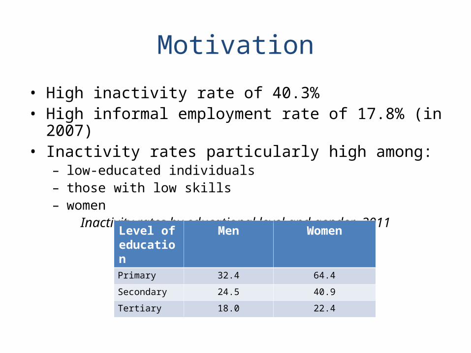
• High inactivity rate of 40.3%• High informal employment rate of 17.8% (in 2007)• Inactivity rates particularly high among:

– low-educated individuals – those with low skills– women

Inactivity rates by educational level and gender, 2011

Level of education

Men Women

Primary 32.4 64.4

Secondary 24.5 40.9

Tertiary 18.0 22.4

Motivation

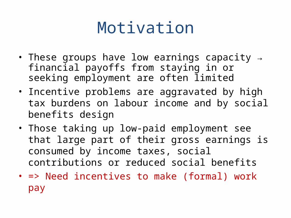
• These groups have low earnings capacity → financial payoffs from staying in or seeking employment are often limited

• Incentive problems are aggravated by high tax burdens on labour income and by social benefits design

• Those taking up low-paid employment see that large part of their gross earnings is consumed by income taxes, social contributions or reduced social benefits

• => Need incentives to make (formal) work pay

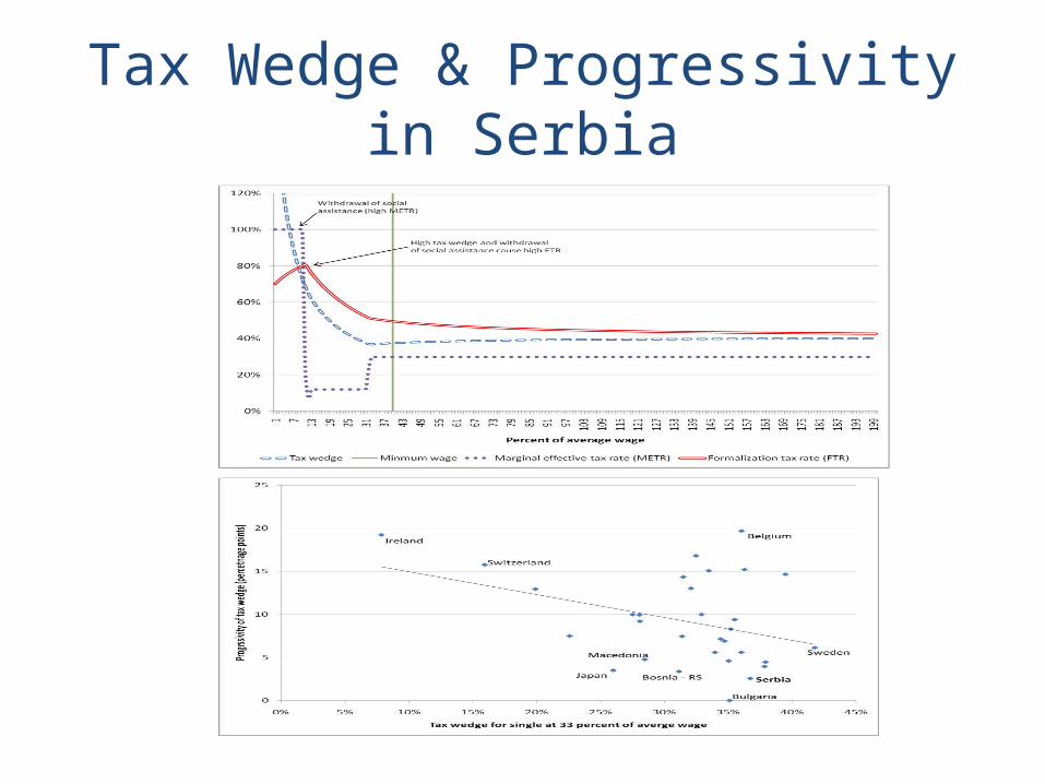
Tax Wedge & Progressivity in Serbia

In-Work Benefits - Purpose

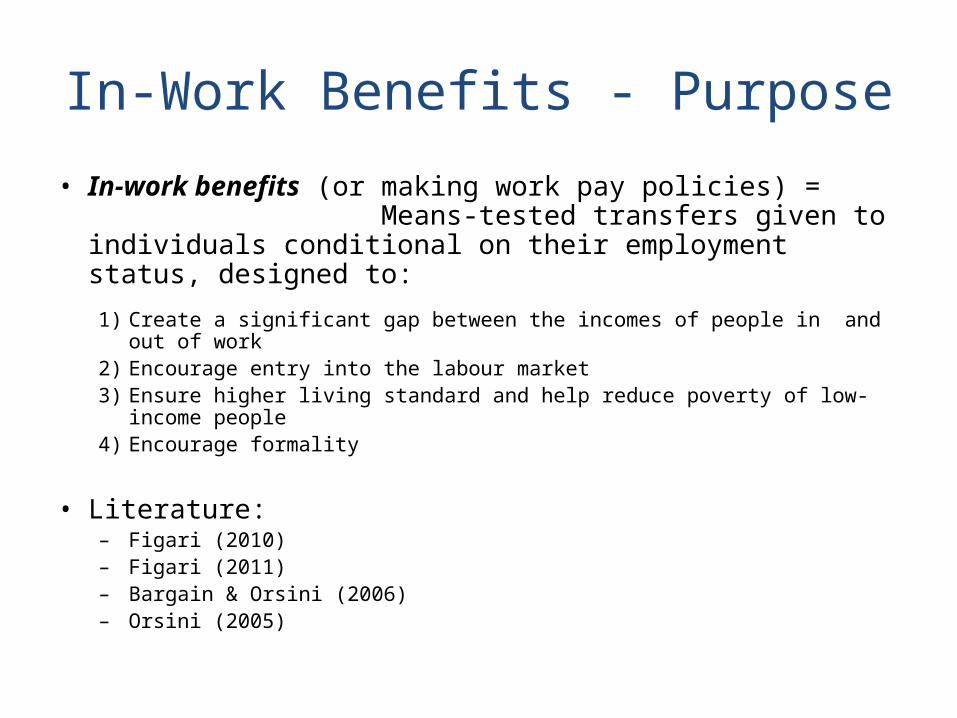
• In-work benefits (or making work pay policies) = Means-tested transfers given to individuals conditional on their employment status, designed to:

1) Create a significant gap between the incomes of people in and out of work 2) Encourage entry into the labour market3) Ensure higher living standard and help reduce poverty of low-income people 4) Encourage formality

• Literature:– Figari (2010)– Figari (2011)– Bargain & Orsini (2006)– Orsini (2005)

WFTC in Serbia – Policy Design (1)

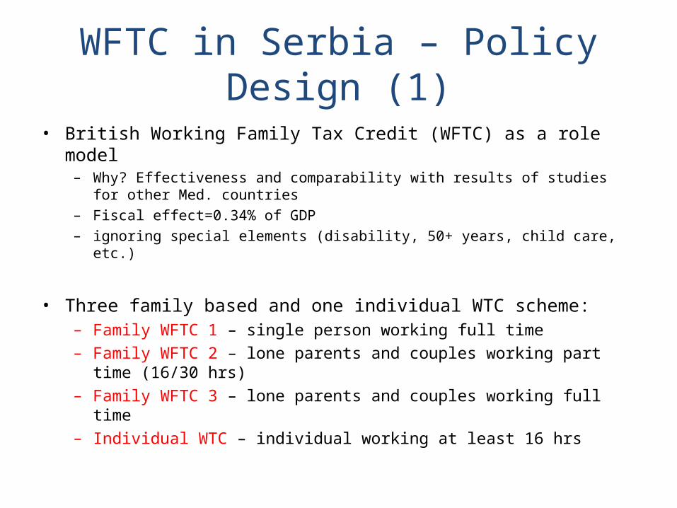
• British Working Family Tax Credit (WFTC) as a role model– Why? Effectiveness and comparability with results of studies for other Med. countries– Fiscal effect=0.34% of GDP– ignoring special elements (disability, 50+ years, child care, etc.)

• Three family based and one individual WTC scheme:– Family WFTC 1 – single person working full time– Family WFTC 2 – lone parents and couples working part time (16/30 hrs)– Family WFTC 3 – lone parents and couples working full time– Individual WTC – individual working at least 16 hrs

WFTC in Serbia – Policy Design (2)

Single working full

time

Lone parents and couples working part

time

Lone parents and couples working full

time

Single working full time

Lone parents and couples working

part time

Lone parents and couples working

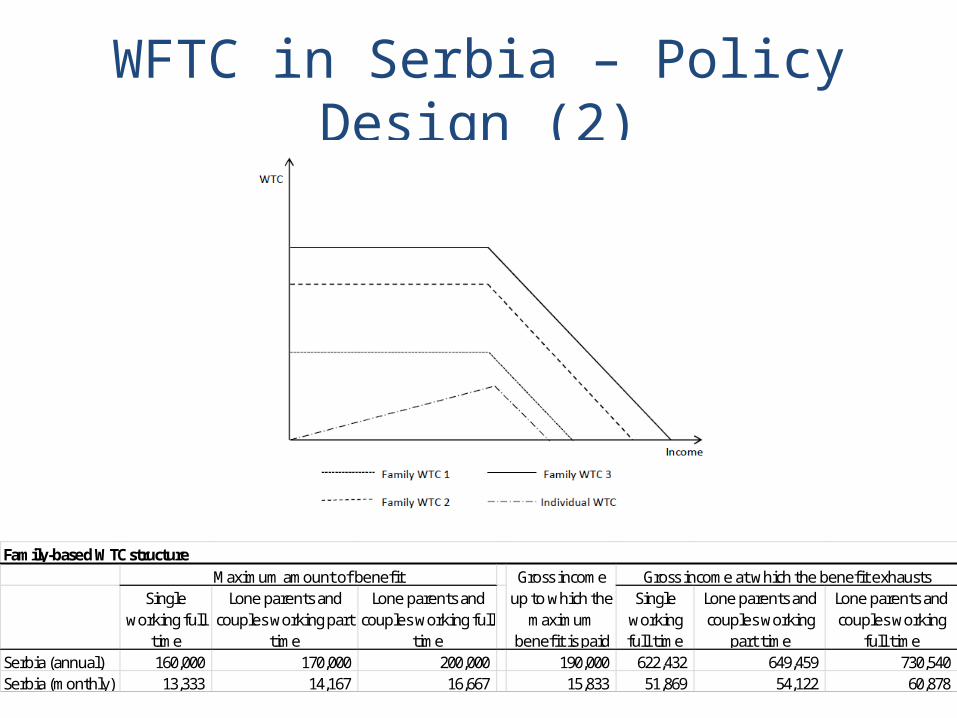
full timeSerbia (annual) 160,000 170,000 200,000 190,000 622,432 649,459 730,540 Serbia (monthly) 13,333 14,167 16,667 15,833 51,869 54,122 60,878

Maximum amount of benefit Gross income up to which the

maximum benefit is paid

Gross income at which the benefit exhaustsFamily-based WTC structure

Aim of the Paper• The most of empirical studies on IWB evaluation focus on

developed countries– ...lack of such studies for transition economies (effects might not be

the same since it depends on the structural features of economy)

• Aims of the paper:– Contribute to empirical literature on labor supply and redistribution

effects of IWB in transition economy • Simulating the effects of introduction of British WTC scheme in Serbia• The first analysis of that kind in Serbia

– Analyze the performances of IWB in transition compared to developed economies with the similar labor market structure

Methodology

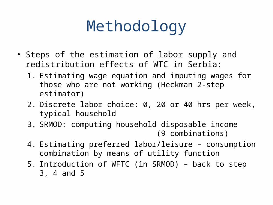
• Steps of the estimation of labor supply and redistribution effects of WTC in Serbia:1. Estimating wage equation and imputing wages for those who

are not working (Heckman 2-step estimator)2. Discrete labor choice: 0, 20 or 40 hrs per week, typical

household3. SRMOD: computing household disposable income

(9 combinations)4. Estimating preferred labor/leisure – consumption combination

by means of utility function5. Introduction of WFTC (in SRMOD) – back to step 3, 4 and 5

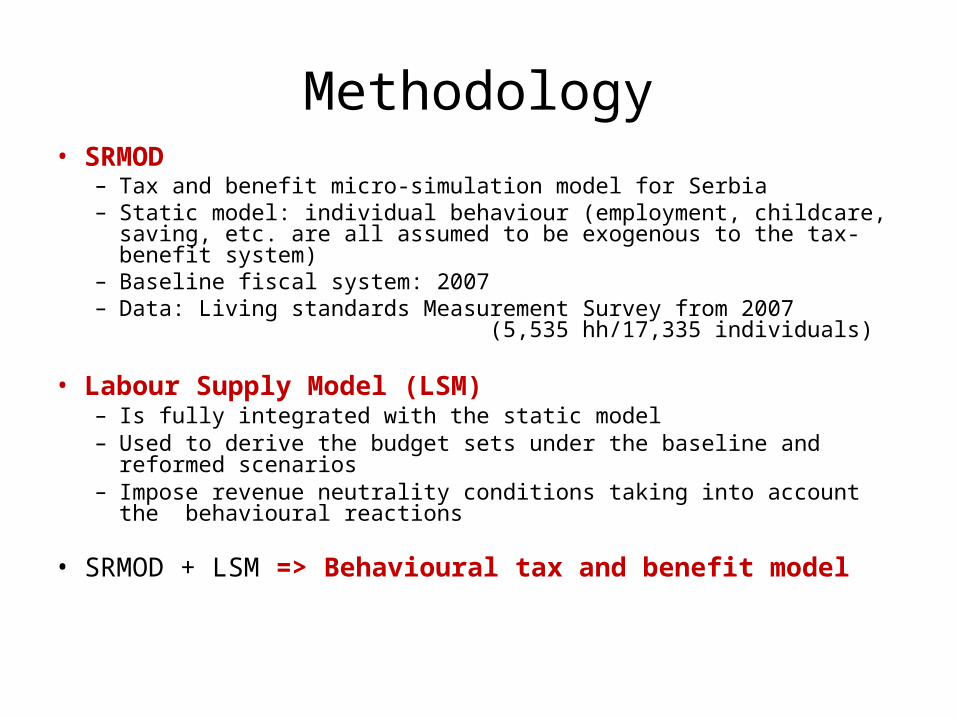
Methodology• SRMOD

– Tax and benefit micro-simulation model for Serbia– Static model: individual behaviour (employment, childcare, saving, etc. are

all assumed to be exogenous to the tax-benefit system)– Baseline fiscal system: 2007– Data: Living standards Measurement Survey from 2007

(5,535 hh/17,335 individuals)

• Labour Supply Model (LSM)– Is fully integrated with the static model– Used to derive the budget sets under the baseline and reformed scenarios– Impose revenue neutrality conditions taking into account the behavioural

reactions

• SRMOD + LSM => Behavioural tax and benefit model

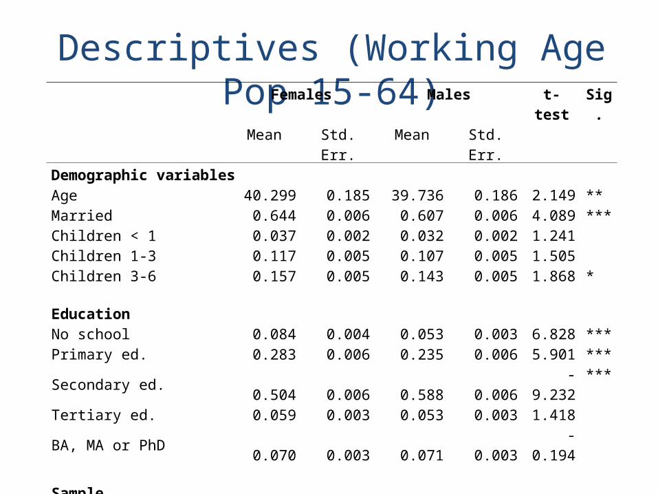
Descriptives (Working Age Pop 15-64)Females Males t-test Sig.

Mean Std. Err. Mean Std. Err.Demographic variablesAge 40.299 0.185 39.736 0.186 2.149 **Married 0.644 0.006 0.607 0.006 4.089 ***Children < 1 0.037 0.002 0.032 0.002 1.241Children 1-3 0.117 0.005 0.107 0.005 1.505Children 3-6 0.157 0.005 0.143 0.005 1.868 *

EducationNo school 0.084 0.004 0.053 0.003 6.828 ***Primary ed. 0.283 0.006 0.235 0.006 5.901 ***Secondary ed. 0.504 0.006 0.588 0.006 -9.232 ***Tertiary ed. 0.059 0.003 0.053 0.003 1.418BA, MA or PhD 0.070 0.003 0.071 0.003 -0.194

SampleUnweighted 5,945 5,826Weighted 2,592,763 2,495,567

1Conditional on being salaried employee2Heckman sample (age 18-64)3Heckman sample (age 18-64) + Conditional on being unemployed or “other inactive“

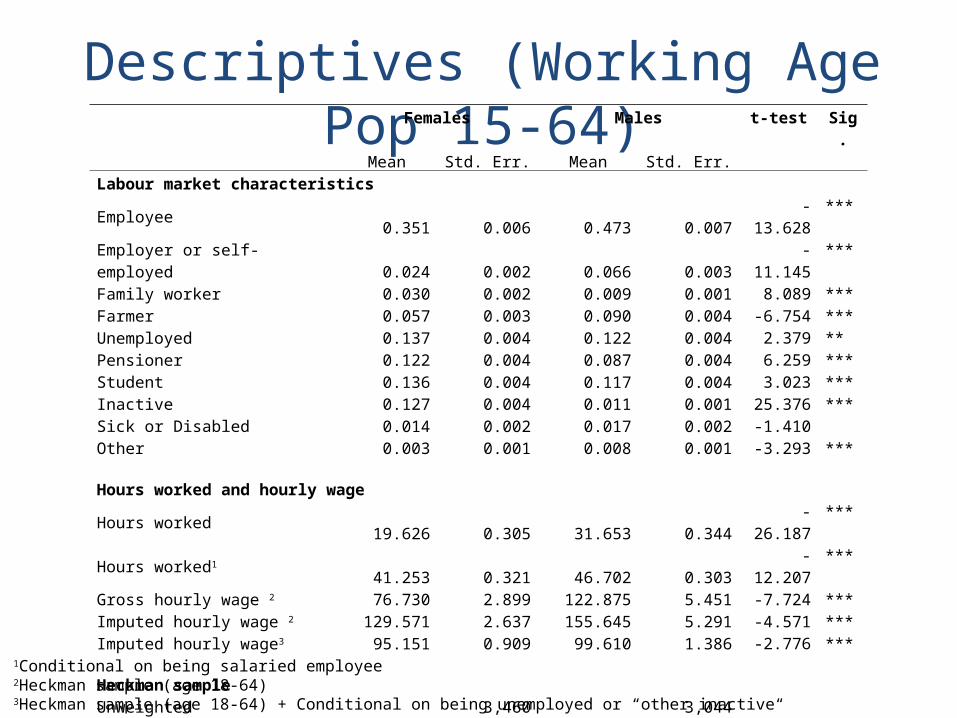
Descriptives (Working Age Pop 15-64)Females Males t-test Sig.

Mean Std. Err. Mean Std. Err.Labour market characteristicsEmployee 0.351 0.006 0.473 0.007 -13.628 ***Employer or self-employed 0.024 0.002 0.066 0.003 -11.145 ***Family worker 0.030 0.002 0.009 0.001 8.089 ***Farmer 0.057 0.003 0.090 0.004 -6.754 ***Unemployed 0.137 0.004 0.122 0.004 2.379 **Pensioner 0.122 0.004 0.087 0.004 6.259 ***Student 0.136 0.004 0.117 0.004 3.023 ***Inactive 0.127 0.004 0.011 0.001 25.376 ***Sick or Disabled 0.014 0.002 0.017 0.002 -1.410Other 0.003 0.001 0.008 0.001 -3.293 ***

Hours worked and hourly wageHours worked 19.626 0.305 31.653 0.344 -26.187 ***Hours worked1 41.253 0.321 46.702 0.303 -12.207 ***Gross hourly wage 2 76.730 2.899 122.875 5.451 -7.724 ***Imputed hourly wage 2 129.571 2.637 155.645 5.291 -4.571 ***Imputed hourly wage3 95.151 0.909 99.610 1.386 -2.776 ***

Heckman sampleUnweighted 3,460 3,044Weighted 1,546,771 1,322,314

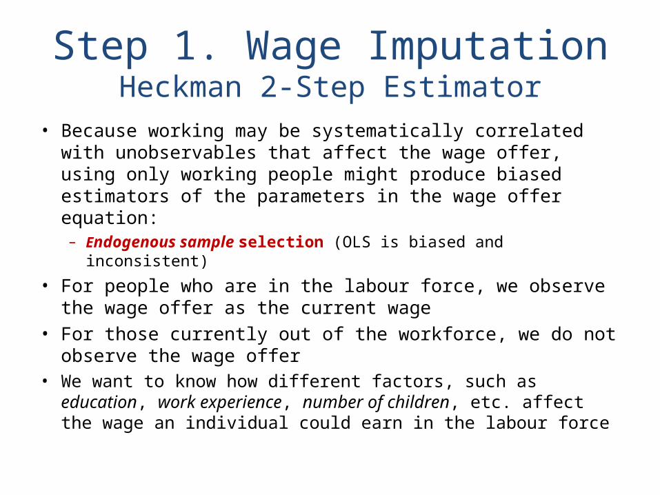
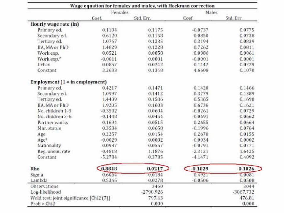
Step 1. Wage ImputationHeckman 2-Step Estimator

• Because working may be systematically correlated with unobservables that affect the wage offer, using only working people might produce biased estimators of the parameters in the wage offer equation:– Endogenous sample selection (OLS is biased and inconsistent)

• For people who are in the labour force, we observe the wage offer as the current wage

• For those currently out of the workforce, we do not observe the wage offer

• We want to know how different factors, such as education, work experience, number of children, etc. affect the wage an individual could earn in the labour force

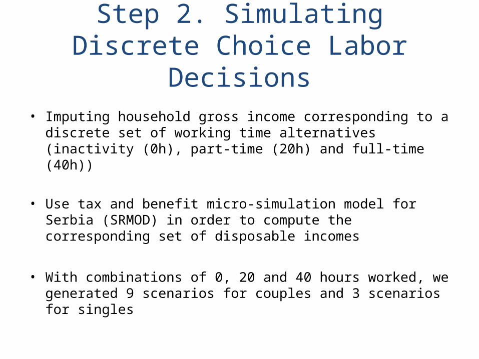
Step 2. Simulating Discrete Choice Labor Decisions

• Imputing household gross income corresponding to a discrete set of working time alternatives (inactivity (0h), part-time (20h) and full-time (40h))

• Use tax and benefit micro-simulation model for Serbia (SRMOD) in order to compute the corresponding set of disposable incomes

• With combinations of 0, 20 and 40 hours worked, we generated 9 scenarios for couples and 3 scenarios for singles

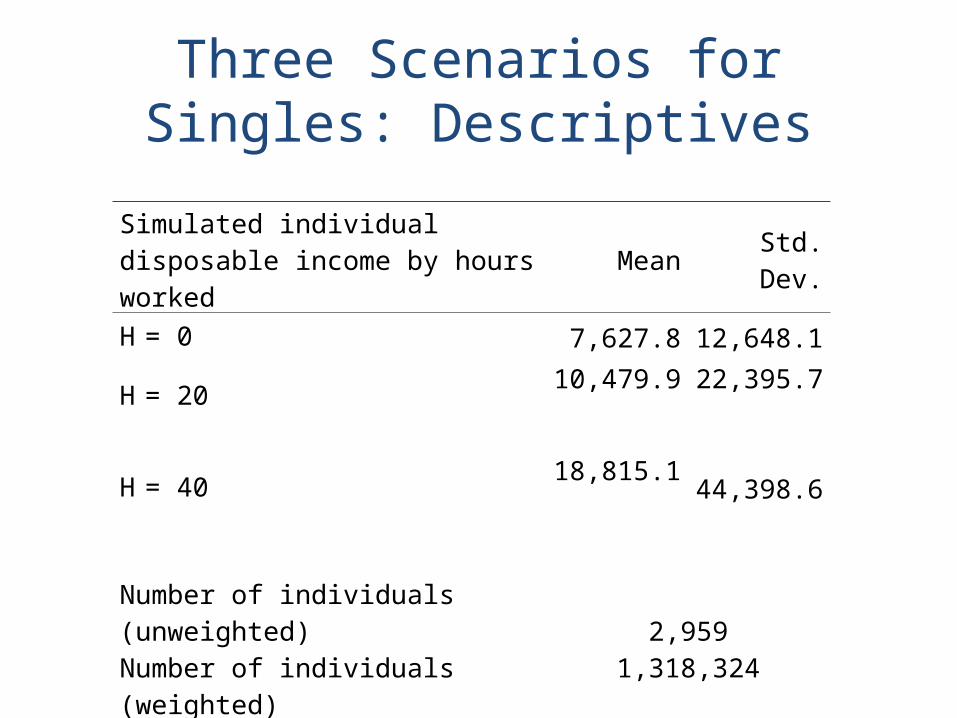
Three Scenarios for Singles: Descriptives

Simulated individual disposable income by hours worked

Mean Std. Dev.

H = 0 7,627.8 12,648.1

H = 20 10,479.9 22,395.7

H = 40 18,815.1 44,398.6

Number of individuals (unweighted)Number of individuals (weighted)

2,9591,318,324

Step 3. Preferences Estimations (1)- Intro -

• Discrete labour supply model (Van Soest, 1995)

• In order to estimate preference parameters in the utility function, we apply simulated maximum-likelihood estimation on a conditional or logit function (McFadden, 1974)– ...we will do the same with mixed logit function

• Direct estimation of preferences over hours and income

• Sample: 1,467 females and 2,595 males

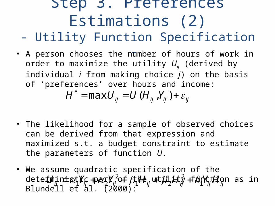
Step 3. Preferences Estimations (2)- Utility Function Specification -

• A person chooses the number of hours of work in order to maximize the utility Uij (derived by individual i from making choice j) on the basis of ‘preferences’ over hours and income:

• The likelihood for a sample of observed choices can be derived from that expression and maximized s.t. a budget constraint to estimate the parameters of function U.

• We assume quadratic specification of the deterministic part of the utility function as in Blundell et al. (2000):

ijijijij YHUUH ),(max*

ijijijijijijij HYHHYYU 12

212

21

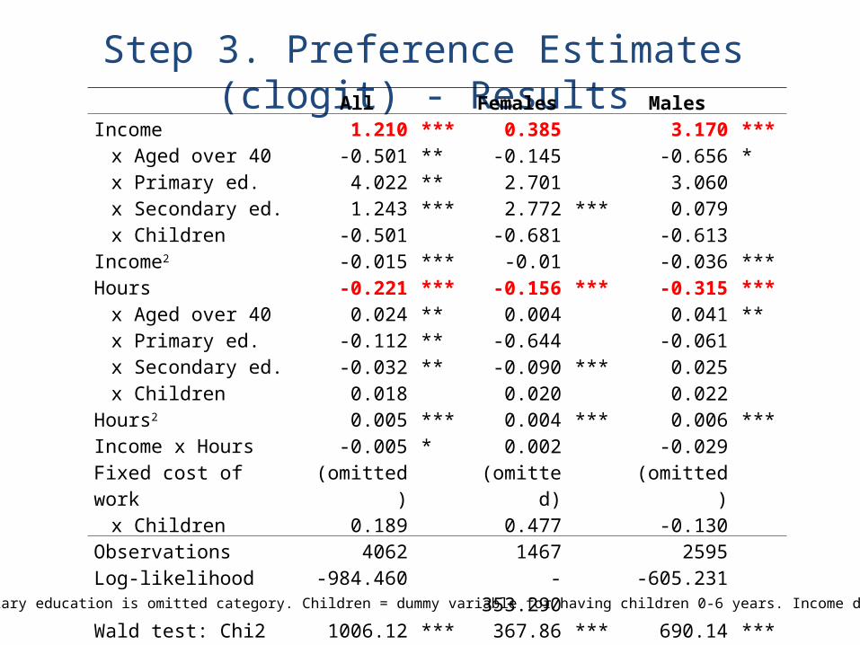
Notes: Tertiary education is omitted category. Children = dummy variable for having children 0-6 years. Income divided by 10,000.

Step 3. Preference Estimates (clogit) - ResultsAll Females Males

Income 1.210 *** 0.385 3.170 ***x Aged over 40 -0.501 ** -0.145 -0.656 *x Primary ed. 4.022 ** 2.701 3.060x Secondary ed. 1.243 *** 2.772 *** 0.079x Children -0.501 -0.681 -0.613

Income2 -0.015 *** -0.01 -0.036 ***Hours -0.221 *** -0.156 *** -0.315 ***

x Aged over 40 0.024 ** 0.004 0.041 **x Primary ed. -0.112 ** -0.644 -0.061x Secondary ed. -0.032 ** -0.090 *** 0.025x Children 0.018 0.020 0.022

Hours2 0.005 *** 0.004 *** 0.006 ***Income x Hours -0.005 * 0.002 -0.029Fixed cost of work (omitted) (omitted) (omitted)

x Children 0.189 0.477 -0.130Observations 4062 1467 2595Log-likelihood -984.460 -353.290 -605.231Wald test: Chi2 (14) 1006.12 *** 367.86 *** 690.14 ***

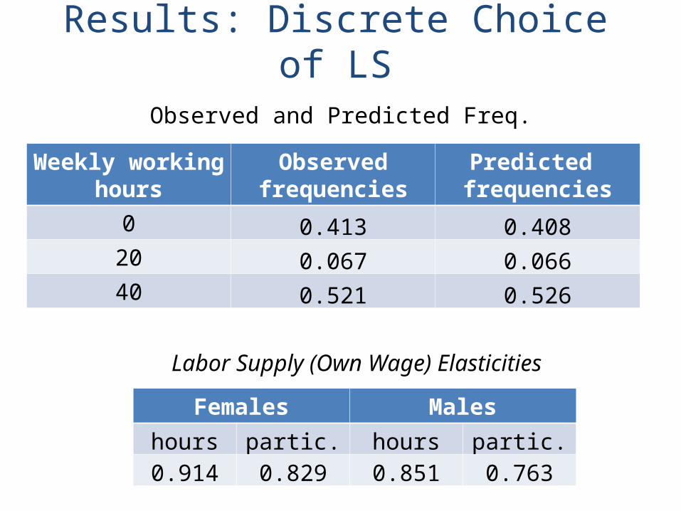
Results: Discrete Choice of LS

Weekly working hours

Observed frequencies

Predicted frequencies

0 0.413 0.40820 0.067 0.06640 0.521 0.526

Labor Supply (Own Wage) Elasticities

Females Males

hours partic. hours partic.0.914 0.829 0.851 0.763

Observed and Predicted Freq.

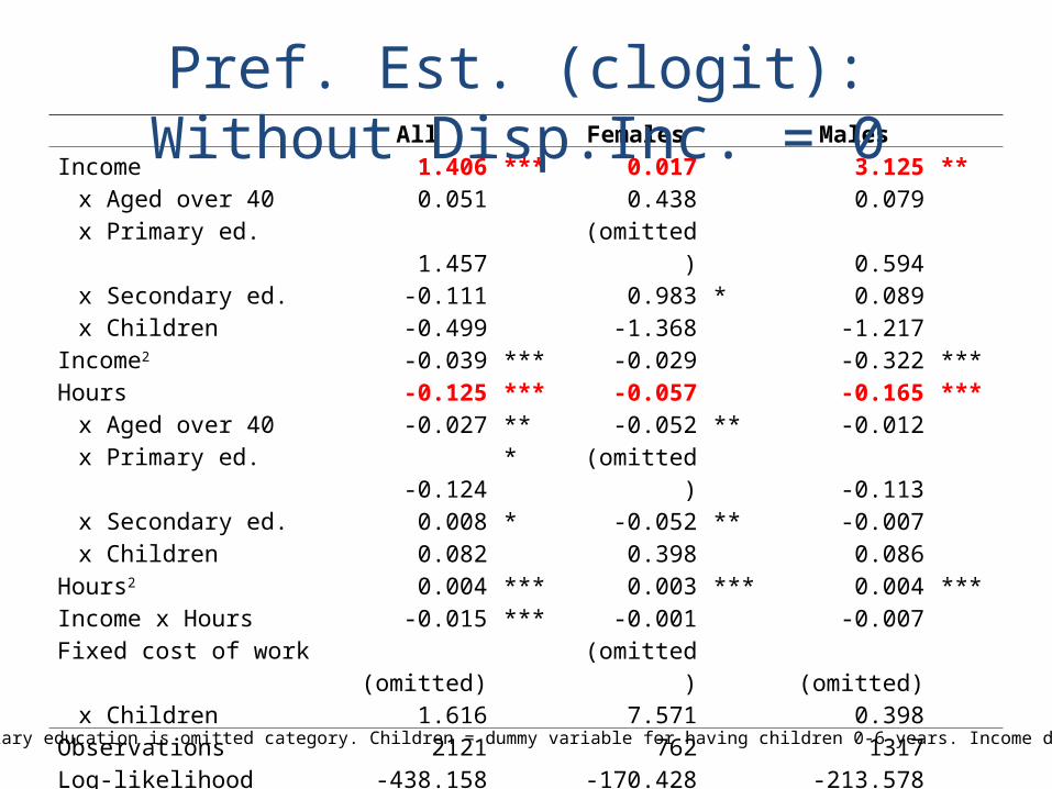
All Females MalesIncome 1.406 *** 0.017 3.125 **

x Aged over 40 0.051 0.438 0.079x Primary ed. 1.457 (omitted) 0.594x Secondary ed. -0.111 0.983 * 0.089x Children -0.499 -1.368 -1.217

Income2 -0.039 *** -0.029 -0.322 ***Hours -0.125 *** -0.057 -0.165 ***

x Aged over 40 -0.027 ** -0.052 ** -0.012x Primary ed. -0.124 * (omitted) -0.113x Secondary ed. 0.008 * -0.052 ** -0.007x Children 0.082 0.398 0.086

Hours2 0.004 *** 0.003 *** 0.004 ***Income x Hours -0.015 *** -0.001 -0.007Fixed cost of work (omitted) (omitted) (omitted)

x Children 1.616 7.571 0.398Observations 2121 762 1317Log-likelihood -438.158 -170.428 -213.578Wald test: Chi2 (14) 699.40 *** 213.31 *** 535.83 ***

Notes: Tertiary education is omitted category. Children = dummy variable for having children 0-6 years. Income divided by 10,000.

Pref. Est. (clogit): Without Disp.Inc. = 0

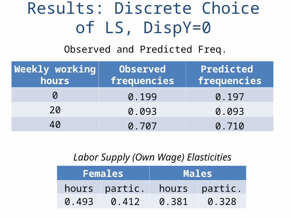
Results: Discrete Choice of LS, DispY=0

Weekly working hours

Observed frequencies

Predicted frequencies

0 0.199 0.19720 0.093 0.09340 0.707 0.710

Labor Supply (Own Wage) Elasticities

Observed and Predicted Freq.

Females Males

hours partic. hours partic.0.493 0.412 0.381 0.328

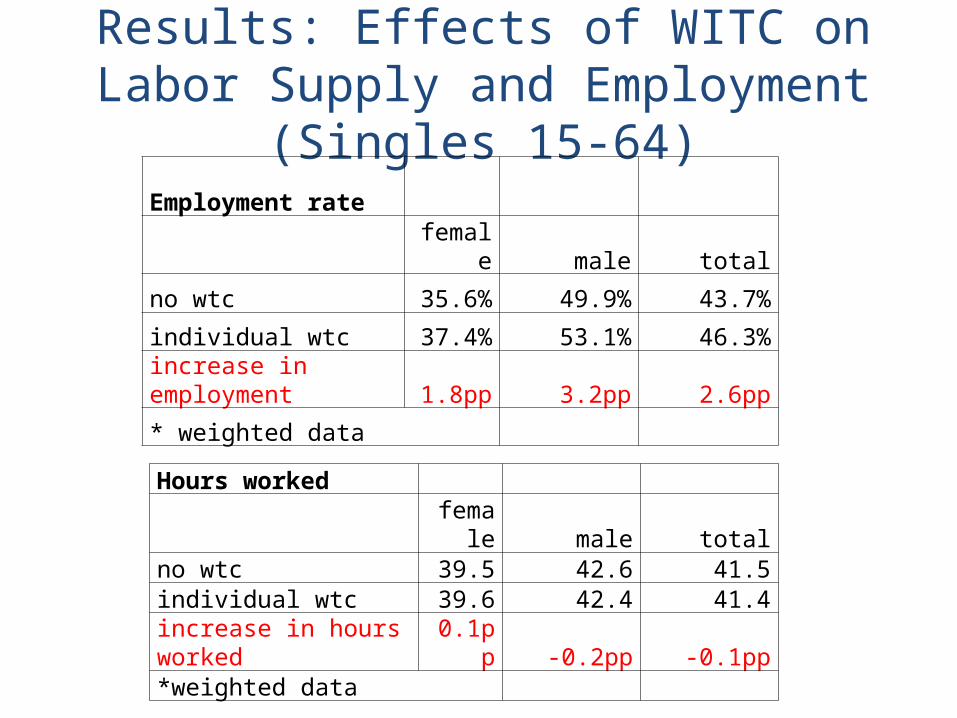
Results: Effects of WITC on Labor Supply and Employment (Singles 15-64)

Employment rate

female male total

no wtc 35.6% 49.9% 43.7%

individual wtc 37.4% 53.1% 46.3%

increase in employment 1.8pp 3.2pp 2.6pp

* weighted data

Hours worked

female male totalno wtc 39.5 42.6 41.5individual wtc 39.6 42.4 41.4increase in hours worked 0.1pp -0.2pp -0.1pp*weighted data

Forthcoming Steps

• Estimating preferences for the couples• Simulation of effects of WFTC• Comparison of the results with other countries

– Portugal, Spain, Italy and Greece?• Figari (2010) – WITC performs better in terms of labor supply, but worse in terms

of inequality than WFTC• The same indication in Serbia (Gini, EMTR)?

– CEE?

• Formulating final conclusions

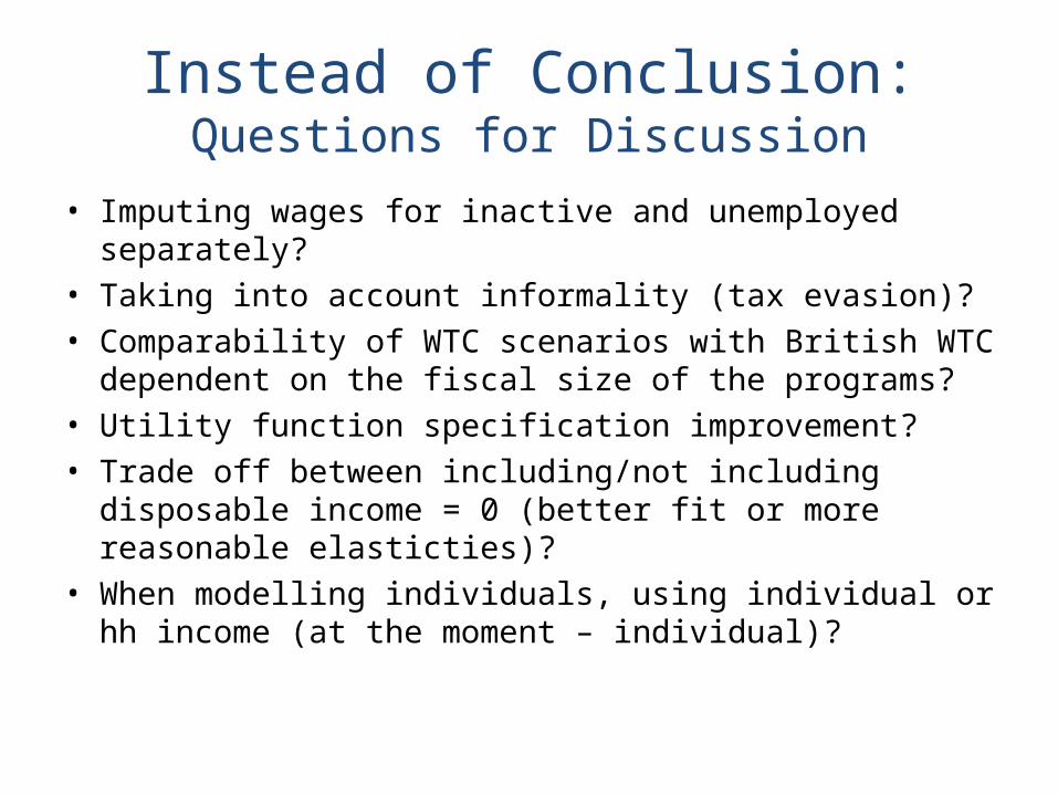
Instead of Conclusion:Questions for Discussion

• Imputing wages for inactive and unemployed separately?• Taking into account informality (tax evasion)?• Comparability of WTC scenarios with British WTC dependent

on the fiscal size of the programs?• Utility function specification improvement?• Trade off between including/not including disposable income

= 0 (better fit or more reasonable elasticties)?• When modelling individuals, using individual or hh income (at

the moment – individual)?

Thank you for your attention!