Malicious Node Identification Scheme for MANET using …€¦ · · 2017-10-13Malicious Node Identification Scheme for MANET using Rough Set Theory S. Sathish Department of Computer

International Journal of Computational Intelligence and Informatics, Vol. 6: No. 3, December 2016

ISSN: 2349 – 6363 172

Malicious Node Identification Scheme for MANET

using Rough Set Theory

S. Sathish Department of Computer Science

Periyar University

Salem, India

[email protected]

M. Saranya Department of Computer Science

Periyar University

Salem, India

[email protected]

Abstract- A mobile ad hoc network is a collection of wireless nodes that can dynamically be set up

anywhere and anytime without using any pre-existing network infrastructure. Due to its nature it has

challenging issues to improve the performance of the network. One of the challenges is to identify the

misbehaving node in the network. The misbehaving nodes plays a vital role in degrade the performance

of the network and may allow the data loss. There are some situations when one or more nodes in the

network become selfish or malicious and tend to annihilate the capacity of the network. The aim of this

work is to detect the malicious nodes using rough set theory. With the help of route cache table the

malicious node are identified based on the transmission history. Every node in the network maintains the

cache table and transmission history about its neighbor node. To find out the transmission history of node

based on transmission metrics calculated such as packet delivery ratio, throughput, end-to-end delay,

number of dropped packet, error rate. To set the source and destination runs the node in simulation

environment with different speeds. Based on the values of transmission history of nodes runs with

different speed are taken to construct the information table. Based on the table the rules are derived to

take a decision whether the nodes are good or bad. After classification apply rough set theory to identify

the malicious node. The path having bad node the packet send an alternate route in a shortest path. Our

experiment results reveals that the rough set based approach increases the network capacity like packet

delivery ratio, as well as decrease end-to-end delay and throughput.

Keywords - Route Cache, Malicious Node, Rough Set, Information Table

1. INTRODUCTION

An Ad hoc network is a collection of mobile nodes, which forms a temporary network without the aid

of centralized administration or standard support devices regularly available as conventional networks (Tao Lin,

2004). These nodes generally have a limited transmission range and, so, each node seeks the assistance of its

neighboring nodes in forwarding packets and hence the nodes in an Ad hoc network can act as both routers and

hosts. Thus a node may forward packets between other nodes as well as run user applications. By nature these

types of networks are suitable for situations where either no fixed infrastructure exists or deploying network is

not possible. Ad hoc mobile networks have found many applications in various fields like military, emergency,

conferencing and sensor networks. Each of these application areas has their specific requirements for routing

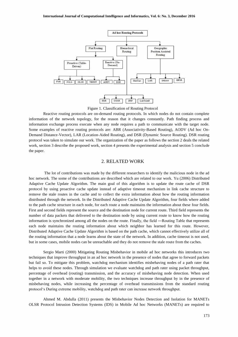
protocols. The routing protocols for ad hoc wireless networks can be broadly classified into four categories

based on Routing information update mechanism, Use of temporal information for routing, Routing Topology,

Utilization of specific resources. Classification of routing protocols shows in the figure 1.

Ad hoc wireless network routing protocols can be classified into three major categories based on the

routing information update mechanism (S.Sathish, 2011)(S.Sathish, 2011). They are: Proactive routing protocols

are also called table–driven routing protocols. They maintain an absolute picture of network at every single node

in the form of tables. These are good for networks which have less node mobility or where nodes transmit data

frequently. DSDV (Destination Sequenced Distance-Vector), WRP (Wireless Routing Protocol), CGSR

(Cluster-head Gateway Switch Routing protocol) and STAR (Source-Tree Adaptive Routing protocol) are some

examples of table-driven routing protocols.


173

Figure 1. Classification of Routing Protocol

Reactive routing protocols are on-demand routing protocols. In which nodes do not contain complete

information of the network topology, for the reason that it changes constantly. Path finding process and

information exchange process execute when any node requires a path to communicate with the target node.

Some examples of reactive routing protocols are: ABR (Associativity-Based Routing), AODV (Ad hoc On-

Demand Distance-Vector), LAR (Location-Aided Routing), and DSR (Dynamic Source Routing). DSR routing

protocol was taken to simulate our work. The organization of the paper as follows the section 2 deals the related

work, section 3 describe the proposed work, section 4 presents the experimental analysis and section 5 conclude

the paper.

2. RELATED WORK

The lot of contributions was made by the different researchers to identify the malicious node in the ad

hoc network. The some of the contributions are described which are related to our work. Yu (2006) Distributed

Adaptive Cache Update Algorithm. The main goal of this algorithm is to update the route cache of DSR

protocol by using proactive cache update instead of adaptive timeout mechanism in link cache structure to

remove the stale routes in the cache and to collect the extra information about how the routing information

distributed through the network. In the Distributed Adaptive Cache Update Algorithm, four fields where added

to the path cache structure in each node, for each route a node maintains the information about these four fields.

First and second fields represent the source and the destination node for current route. Third field represents the

number of data packets that delivered to the destination node by using current route to know how the routing

information is synchronized among all the nodes on the route. Finally, the field ―Routing Table that represents

each node maintains the routing information about which neighbor has learned for this route. However,

Distributed Adaptive Cache Update Algorithm is based on the path cache, which cannot effectively utilize all of

the routing information that a node learns about the state of the network. In addition, cache timeout is not used,

but in some cases, mobile nodes can be unreachable and they do not remove the stale route from the caches.

Sergio Marti (2000) Mitigating Routing Misbehavior in mobile ad hoc networks this introduces two

techniques that improve throughput in an ad hoc network in the presence of nodes that agree to forward packets

but fail so. To mitigate this problem, watchdog mechanism identifies misbehaving nodes of a path rater that

helps to avoid these nodes. Through simulation we evaluate watchdog and path rater using packet throughput,

percentage of overhead (routing) transmission, and the accuracy of misbehaving node detection. When used

together in a network with moderate mobility, the two techniques increase throughput by in the presence of

misbehaving nodes, while increasing the percentage of overhead transmissions from the standard routing

protocol‘s During extreme mobility, watchdog and path rater can increase network throughput.

Ahmed M. Abdulla (2011) presents the Misbehavior Nodes Detection and Isolation for MANETs

OLSR Protocol Intrusion Detection Systems (IDS) in Mobile Ad hoc Networks (MANETs) are required to


174

develop a strong security scheme it is therefore necessary to understand how malicious nodes can attack the

MANETs. Focusing on the Optimized Link State Routing (OLSR) protocol, an IDS mechanism to accurately

detect and isolate misbehavior node(s) in OLSR protocol based on End-to-End (E2E) communication between

the source and the destination is proposed. The collaboration of a group of neighbor nodes is used to make

accurate decisions. Creating and broadcasting attackers list to neighbor nodes enables other node to isolate

misbehavior nodes by eliminating them from the routing table. Eliminating misbehavior node allows the source

to select another trusted path to its destination.

Feng Li (2010) proposes Enhanced Intrusion Detection System for Discovering Malicious Nodes in

Mobile Ad hoc Networks as mobile wireless ad hoc networks have different characteristics from wired networks

and even from standard wireless networks, there are new challenges related to security issues that need to be

addressed. Many intrusion detection systems have been proposed and most of them are tightly related to routing

protocols, such as Watchdog/Path rater and Route guard. These solutions include two parts: intrusion detection

(Watchdog) and response (Path rater and Route guard). Watchdog resides in each node and is based on

overhearing. Through overhearing, each node can detect the malicious action of its neighbors and report other

nodes. However, if the node that is overhearing and reporting itself is malicious, then it can cause serious impact

on network performance. In this mechanism overcome the weakness of Watchdog and introduce our intrusion

detection system called Watchdog. It has ability to discover malicious nodes which can partition the network by

falsely reporting, other nodes as misbehaving and then proceeds to protect the network.

Mohit Jain (2014) proposes A Rough Set Based Approach to Classify Node Behavior in Mobile Ad

Hoc Network there are some situations when one or more nodes in the network become selfish or malicious and

tend to annihilate the capacity of the network. This investigate the classification of good and bad nodes in the

network by using the concept of rough set theory, that can be employed to generate simple rules and to remove

irrelevant attributes for discerning the good nodes from bad nodes.

AnshuChauhan (2015) describes the Detection of Packet Dropping Nodes in MANET using DSR

Routing Protocol. The approach is used to identify the malicious node can establish monitoring of neighbor

concept. But every node will not be the monitoring node because in mobile ad hoc network every node has

limited battery power so every node should not be in listening mode it will degrade its service time. Firstly will

create some overlapping clusters and each cluster will be having on monitoring node. These monitoring nodes

will detect packet dropping nodes in their zone area and maintain trust information about each node of their

zone and will provide this information to the source node as well as other cluster‘s monitoring node whenever

required. This mechanism divides the whole network onto some small virtual zones and for each zone only one

monitoring node is being selected to detect the packet droppers. So some advantages with this mechanism are:

its false detection rate is low and overhead on the network is also less. Simulation shows that a better packet

delivery ratio and throughput has been gained again after prevention mechanism. Thus we have successfully

injected, detected and also avoided packet dropping nodes from the path of DSR.

3. MALICIOUS NODE IDENTIFICATION SCHEME FOR MANET USING ROUGH SET

THEORY

3.1. DSR Cache Table

Cache table is a data structure that maintains the record of routing information of each node that is

useful for cache updates. A cache table has no capacity limit; its size increases as new routes are discovered and

decreases as stale routes are removed (Yu, 2006). There are four fields in a cache table entry: Route, Source

Destination, Data Packets and Reply Record. In the field of Route stores the links starting from the current node

to a destination or from a source to a destination. Source Destination: It is the source and destination pair. Data

Packets: It records whether the current node has forwarded data packets. Reply Record: This field may contain

multiple entries and has no capacity limit. Replies from caches provide dual performance advantages. First, they

reduce route discovery latency. Second, without replies from caches the route query flood will reach all nodes in

the network (request storm).


175

3.2. Route Cache

The route cache is used in DSR protocol to store all the routes are learned from the source node to the

destination and to avoid unnecessary route discovery process. Thus the cache will behave as the current

topology of the network (Bin Xiao, 2003). Because that reinitiating of a route discovery mechanism in on

demand routing protocols is very costly in term of delay, battery power, and bandwidth consumption due to

flooding of the network, which can cause long delay before the first data packet sent. The performance of

protocols mainly depends on an efficient implementation of route cache. When an invalid route cache is used,

extra traffic overheads and routing delays are incurred to discover the broken links. One approach to minimize

the effect of invalid route cache is to purge the cache entry after some Time-to-Live (TTL) interval. If the TTL

is set too small, valid routes are likely to be discarded, and large routing delays and traffic overheads may result

due to the new route search. The routes are stored in the cache to avoid unnecessary route discovery for

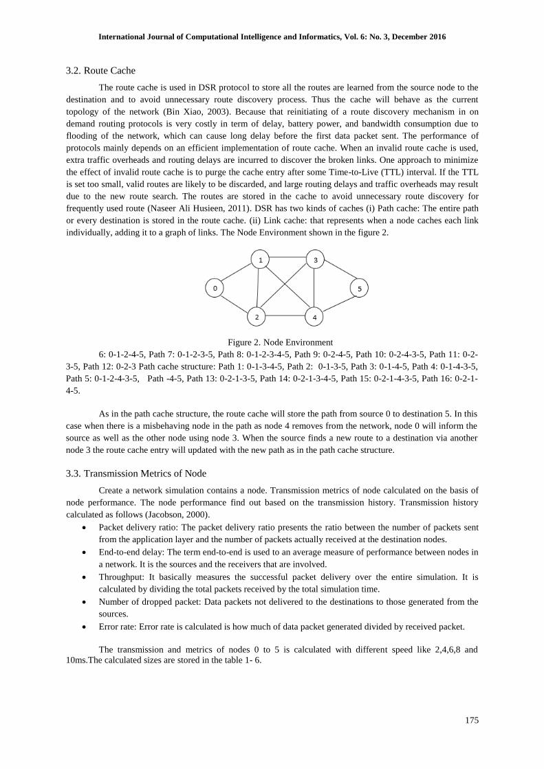
frequently used route (Naseer Ali Husieen, 2011). DSR has two kinds of caches (i) Path cache: The entire path

or every destination is stored in the route cache. (ii) Link cache: that represents when a node caches each link

individually, adding it to a graph of links. The Node Environment shown in the figure 2.

Figure 2. Node Environment

6: 0-1-2-4-5, Path 7: 0-1-2-3-5, Path 8: 0-1-2-3-4-5, Path 9: 0-2-4-5, Path 10: 0-2-4-3-5, Path 11: 0-2-

3-5, Path 12: 0-2-3 Path cache structure: Path 1: 0-1-3-4-5, Path 2: 0-1-3-5, Path 3: 0-1-4-5, Path 4: 0-1-4-3-5,

Path 5: 0-1-2-4-3-5, Path -4-5, Path 13: 0-2-1-3-5, Path 14: 0-2-1-3-4-5, Path 15: 0-2-1-4-3-5, Path 16: 0-2-1-

4-5.

As in the path cache structure, the route cache will store the path from source 0 to destination 5. In this

case when there is a misbehaving node in the path as node 4 removes from the network, node 0 will inform the

source as well as the other node using node 3. When the source finds a new route to a destination via another

node 3 the route cache entry will updated with the new path as in the path cache structure.

3.3. Transmission Metrics of Node

Create a network simulation contains a node. Transmission metrics of node calculated on the basis of

node performance. The node performance find out based on the transmission history. Transmission history

calculated as follows (Jacobson, 2000).

Packet delivery ratio: The packet delivery ratio presents the ratio between the number of packets sent

from the application layer and the number of packets actually received at the destination nodes.

End-to-end delay: The term end-to-end is used to an average measure of performance between nodes in

a network. It is the sources and the receivers that are involved.

Throughput: It basically measures the successful packet delivery over the entire simulation. It is

calculated by dividing the total packets received by the total simulation time.

Number of dropped packet: Data packets not delivered to the destinations to those generated from the

sources.

Error rate: Error rate is calculated is how much of data packet generated divided by received packet.

The transmission and metrics of nodes 0 to 5 is calculated with different speed like 2,4,6,8 and

10ms.The calculated sizes are stored in the table 1- 6.


176

Table : 1 Transmission history of node 0 runs with different speed

Speed

@ ms

Packet

delivery

ratio

End-to-

End

delay

Throughput

Number of

dropped

packet

Error

Rate

@2 99.9735 15.590 754.79 0 1

@4 98.5046 17.302 751.53 12 0.9898

@6 98.0074 20.920 752.53 10 0.9847

@8 98.0001 25.422 755.91 15 0.9798

@10 98.5790 20.044 753.67 20 0.9885


Speed

@ ms

Packet

delivery

ratio

End-

to-end

delay

Throughput

Number of

dropped

packet

Error

Rate

@2 99.9333 21.732 755.78 12 0.998

@4 99.0007 17.866 752.78 15 0.992

@6 98.7237 24.093 755.91 16 0.989

@8 98.0002 23.598 752.91 20 0.974

@10 98.8441 39.733 753.67 25 0.980


Speed

@ ms

Packet

delivery

ratio

End- to-

end

delay

Throughput

Number of

dropped

packet

Error

Rate

@2 92.210 27.205 755.78 15 0.993

@4 94.589 30.437 755.91 20 0.938

@6 94.215 32.971 752.53 22 0.843

@8 94.002 33.394 753.67 25 0.981

@10 94.235 38.336 751.61 20 0.103


Speed

@ ms

Packet

delivery

ratio

End-to-

end

delay

Throughput

Number of

dropped

packet

Error

Rate

@2 85.2160 52.687 755.78 20 0.578

@4 80.0013 50.992 752.91 15 0.993

@6 82.5526 35.456 753.61 16 0.843

@8 80.5756 57.012 752.53 50 0.981

@10 80.0005 68.117 750.61 11 0.103


Speed

@ ms

Packet

delivery

ratio

End-to-

end

delay

Throughput

Number

of

dropped

packet

Error

Rate

@2 80.216 66.006 750.61 15 0.988

@4 77.482 65.408 750.93 50 0.980

@6 77.497 62.249 751.61 40 0.103

@8 75.827 80.001 752.83 60 0.027

@10 70.762 72.885 753.27 52 0.008


177


Speed

@ ms

Packet

delivery

ratio

End-to-

end

delay

Throughput

Number of

dropped

packet

Error

Rate

@2 99.933 15.590 755.79 2 0.993

@4 98.002 20.920 751.53 4 0.938

@6 98.841 25.422 752.53 12 0.843

@8 98.723 17.302 753.67 8 0.981

@10 99.007 30.044 755.91 20 0.986

3.4. Information System of Rough Set Theory

3.4.1 Rough set theory

Rough set theory proposed by Pawlak (1982) is a mathematical tool that’s deals with vagueness and

uncertainty. Its concepts and operations are defined based on the indiscernibility relation. In this theory, a data

set is represented as a table, where each row represents an event or object or an example or an entity or an

element. Each column represents an attribute that can be measured for an element. (Sheikh, 2010),(Usman

Singh, 2011). this data table is known as Information systems. The set of all elements is known as universe it

has been successfully applied in selecting attributes to improve the efficiency in deriving decision rules. In

Information systems, elements that have the same value for each attribute are indiscernible and are called

elementary sets. Subsets of the universe with the same value of the decision attribute are called concepts. A

positive element is an element of the universe that belongs to concept. For each concept, the greatest union of

elementary sets contained in the concept is called the lower approximation of the concept and the least union of

elementary sets contain the concept is called the upper approximation of the concept, that are not the members

of the lower approximation is called the boundary region. It provides the useful information about the role of

particular attributes and their subsets and prepares the ground for representation of knowledge hidden in data by

means of IF-THEN decision rules. A set is said to be rough if the boundary region is non-empty and a set is said

to be crisp if the boundary region is empty.

3.4.2 Information System

An information system can be viewed as a table where each row presents an object and each column

present attribute. That can be measured for each object. Basically, an information system is a pair S = (U, A)

where U in non-empty finite set of object known as universe and A is non empty finite set of attributes such that

a: U → Va for every a ∈ A and the set Va is called the value set of a (Jacobson, 2000). Information system can be

extended by the inclusion of decision attributes and information systems of this kind are known as decision

systems. A decision system is an information system of the form S = U, A, U d , whered ∉ A. Information

systems can be extended by the inclusion of decision attributes and information systems of this kind is known as

decision systems. A decision system is an information system of the form S = U, A, U d , whered ∉ A. Is the

decision attributes and the elements of A are called condition attributes. Normally decision attribute takes one of

two possible Values but it can also take multi values. A decision system expresses almost all the knowledge

about the model. Sometimes in the data table the same or indiscernible objects may be represented several

times or some of the attributes may be superfluous. This can be expressed as equation (1).

IND B = X, X′ ∈ U2 ∀a∈ B a x = a x′ (1)

Where IND(B) is an equivalence relation and is called B-indiscernibility relation. Rough set analysis

can be done using lower and upper approximations. This can be defined as follows.

Lower approximation

B∗ X = X ∈ U: B X ⊆ X (2)


178

Upper approximation

B∗ X = X ∈ U: B X ∩ X ≠ ϕ (3)

Where B ⊆ A and X ⊆ U. We can approximate X by using only the Information contained in B by

constructing the lower approximation and Upper approximation defined in (2) and (3). Due to granulity of

knowledge, rough sets cannot be characterized by using Available knowledge. Therefore with every rough set

we associate two crisp called its lower and upper approximation. The lower approximation of sets consists of all

elements that surely belong to the set. The difference of the upper and lower approximation is a boundary region

and any rough set has non empty set boundary region. Rough sets can be characterized numerically by the

coefficient as in the equation (4).

αB X =|B∗ X |

|B∗ X | (4)

where |X| denote the cardinality X = ϕ. If αB X = 1, the set X is crisp with respect to B and

ifαB X < 1, the set X is rough with respect to B.

Sometimes there are some subsets of conditional attribute that preserve the portioning of the universe

and such subsets are known as minimal reducts. Such reducts can be finding with the help of discernibility

matrix function which can be defined in equation 5:

Cij = a ∈ A a xi ≠ a xj for i, j = 1 …… n

a1∗ …… . am

∗ = Λ{V Cij∗ |1 ≤ j ≤ i ≤ n, Cij ≠ ∅ (5)

where Cij∗ = {a∗|a ∈ Cij }. Also we can measure the significance of the approximate reduct and the

effect on the data set after dropping that particular attribute by the formula in equation (6)

∝(C,D)= 1 − γ(C − α ,D

γ C,D (6)

The information system is shown in a Table 7. Where each row represent an object and each column

represent an attributes. The below table 7 represents the average values of the nodes behavior.

Table : 7 Average values of nodes based on the transmission history runs with different speed

Nodes

Packet

delivery

ratio

End-to-

end

delay

Throughput

Number of

dropped

packet

Error

Rate

0 98.6123 21.85 753.686 10.5 0.984

1 98.9034 25.40 754.134 14.0 0.986

2 93.8501 32.46 753.900 17.0 0.771

3 81.6692 45.76 753.088 18.6 0.705

4 76.3573 69.30 751.850 36.1 0.416

5 98.9003 21.85 753.886 16.4 0.948

Derive IF-THEN decision rules from average values of all the nodes based on the transmission history

runs with different speed.

If Packet delivery ratio>= 95 and then decision=high

Else if packet delivery ratio>= 81 then decision =medium

Else if packet delivery ratio≤80 then decision=low


179

If end-to-end delay≤45 then decision=low

Else if end-to-end delay>50 then decision=high

If Throughput>753 then decision=high

Else if throughput<750 then decision=low

If Number of dropped packet<=10 then decision=low

Else if number of dropped packet<=20 then decision=medium

Else if number of dropped packet>25 then decision=high

If error rate≤0.984 then decision=low

Else if error rate=0.986 then decision=medium

Else if error rate=0.416 then decision=high

Table : 8 Data Set

Nodes PDR

End-to-

End

delay

Throughput

No. of

Dropped

Packet

Error

Rate Decision

0 H L H L L GOOD

1 H L H L M GOOD

2 H L H M L GOOD

3 M L H L L GOOD

4 L H L H H BAD

5 H L H L L GOOD

The above rules are used to classify the nodes behavior such as good or bad. If PDR=High/medium,

End-to-End delay=Low, Throughput=high, No. of dropped packet=Low/medium, error rate=Low/medium then

decision=Good. Else if PDR=Low, End-to-End delay=high, Throughput=Low, No. of dropped packet=High,

Error Rate=High then decision=Bad.

3.5. Node Classification Using Rough Set Theory

The nodes are classified as good node or bad node based on the performance metrics of each node such

as Packet delivery ratio, end-to- end delay, Throughput, Number of dropped packet, Error rate. Table 8 shows

the classification of various nodes and in addition to this H refers High, M refers Medium and L refers Low.

3.6. Analysis of Data Using RSES

In this dissertation using RSES (Rough Set Exploration System) to obtain decision rules and we will

apply these rules to the network scenario containing malicious nodes to detect it. RSES is a toolkit for analysis

of table data based on methods and algorithms coming from the area of rough sets (Usman Singh, 2011). We

will ensure the following steps in order to implement our proposed work to detect the malicious nodes.

Procedure:

Step1: Load data to the RSES.

Step2: Find the Reduct.

Step3: Derive the Decision rules.

Step4: Use the Classifier known as Decision trees to learn from the training data set.

Step 5: Build the confusion matrix.

Step6: Apply the derived the decision rules to detect the malicious nodes


180

3.7. Malicious Node Identification

The average value of transmission metrics are considered in order to classify the nodes based on the

decision rules. The classified nodes describe the characteristics of the each node whether it is good or bad. In

order to identify the bad nodes in the network, the rough set theory are used and the different simulation are

considered with different speed. The malicious nodes of network are identified, and remove that malicious node

in the path cache. The updated path cache tables are used for routing process. The following procedure is used

to identify the malicious nodes in the network.

Procedure for Malicious node identification:

Step 1: create a network simulation with 6 nodes.

Step 2: To find the transmission metrics of a node such as

Packet delivery ratio:

PDR = No. of packets Received No. of packet send X100

End-to-End delay:

delay = arrive time − send time / No. of Connections

Throughput:

Throughput = Received size start time − stop time X8/100

Number of dropped packet:

NDP = Dpackets

Error rate of node:

Error Rate =Received Packet

Generated Packet

Step 3: Perform the simulation with different speed for every node to calculate the transmission metrics

of an each node.

Step 4: Derive decision rules based on the transmission metrics

Step 5: classify the node whether good or bad, based on the rule.

Step 6: Generate the information table from the transmission metrics table and apply rough set theory

to identify the malicious node

Step 7: Remove the malicious node in the cache table and update the cache table.

Step 8: Perform the routing process.

4. EXPERIMENTAL RESULTS AND ANALYSIS

4.1. Simulation Environment

Network Simulator (NS2) is a discrete event driven simulator developed at UC Berkeley. It is part of

the VINT project. The goal of NS2 is to support networking research and education. It is suitable for designing

new protocols, comparing different protocols and traffic evaluations. NS2 is developed as a collaborative

environment. It is distributed freely and open source. A large amount of institutes and people in development

and research use, maintain and develop NS2.

Table : 9 Simulation Environment

Simulation Parameters

Routing Protocols DSR

Simulation Time 500 sec

Number of Nodes 6

Simulation Area 1500 X 1500

Pause tine 20 sec

Traffic Type CBR

Packet Size 512 Bytes

Rate 10 packets/sec


181

Simulation environment consists of 6 wireless mobile nodes which are placed uniformly and forming a

mobile ad hoc network, moving about over a 1500 x 1500 meters area for 500 seconds of simulated time. All

mobile nodes in the network are configured to run dynamic Source Routing protocol (DSR). For the

experiments in this paper; constant bit rate (CBR) traffic sources are used. The simulation parameters mentioned

the table 9.

4.2. Performance Metrics

To correspond to the special distinctiveness and recital of network following metrics are used in our

simulation:

Throughput: It basically measures the successful packet delivery over the entire simulation. It is

calculated by dividing the total packets received by the total simulation time. Throughput = Pr / (T2 -

T1). Where, Pr is total data size received, T1 is the start time and T2 is the stop time of simulation.

Packet Delivery Ratio: PDR is the ratio between the number of packets transmitted by a traffic source

and the number of packets received by a traffic sink. A high PDR is desired in a network. PDR = (Pr /

Ps) * 100 Where, Pr is total packets received and Ps is the total packets sent.

Average end-to-end Delay: The packets end-to-end delay is the average time that packets have to pass

through the network. It represents the reliability of routing protocols. Delay = (T2 – T1) where, T2 is

receive time and T1 is sent time.

4.3. Result and Analysis

Performance analysis of existing and proposed work is shown in the figure 3 and table 10.

Table : 10 Performance analysis

Analysis

Packet

delivery

ratio (%)

Throughput

(kpbs)

End-to-

End

Delay(ms)

Existing 97.003 753.91 20.53

Proposed 99.753 250.53 15.33

Figure 3. Performance analysis

97.003

753.91

20.53

99.753

250.53

15.33

0

100

200

300

400

500

600

700

800

Packet delivery ratio Throughput End-to-End delay

Performance analysis

Existing work

proposed work


182

5. CONCLUSION AND FUTURE WORK

Security is always an open area of research and improvement. The configuration of security mechanism

in ad hoc network is a challenging task due to its dynamic nature and resources constrains. This work describes

how packet dropper’s nodes on the network have drastically degraded the network performance. With the help

of route cache table the malicious node are identified based on the transmission history. Every node in the

network maintains the cache table and transmission history about its neighbor node. Based on the transmission

history the nodes are classified using rough set theory whether the nodes are good or bad. Rough set methods

helps in removing the superfluous attributes and gives the minimal set of attributes known as reduct by

preserving the partition of the universe of discourse and generate the decision rules. To derive the decision rules

for classify the nodes. If path having malicious node. The packet forwarder takes an alternative path and shortest

path. Thus we have successfully injected, detected and also avoided packet dropping nodes from the path of

DSR. Route breakup can easily recover since path cache established. Some advantages with this mechanism are:

false detection rate is low and overhead on the network is also less. Simulation shows that packet delivery ratio

throughput and end to end delay has been gained again after prevention mechanism.

The ad hoc networking is an open challenging area of research in computer science due to its dynamic

nature. This means adhoc network contains lots of vulnerabilities to be explored and many other issues to be

solved. In future our plan is to study some other vulnerable areas of mobile and hoc network. We will also try to

configure this proposed mechanism with other mechanism such as neural network, fuzzy set and hybrid models

to identify the malicious node in the network.

REFERENCES

Ahmed M. Abdulla, I. A. (2011). Misbehavior Nodes Detection and Isolation for MANETs OLSR Protocol.

Science Direct:World Conference on Information Technology, 115-121.

AnshuChauhan, D. (2015). Detection of Packet Dropping Nodes in MANET using DSR Protocol. International

Journal of Computer Applications, 123 (7), 0975-8887.

Bin Xiao, Q. F. (2003). Enhanced Route Maintenance for Dynamic Source Routing in Mobile Ad Hoc

Networks.

Feng Li, Y. Y. (2010). Attack and Flee: Game-Theory- Based Analysis on Interactions among Nodes in

MANETs. IEEE Transactions on Systems Man and Cybernetics, 40 (3).

Jacobson, A. (2000). Metrics in MANET, Lulea University of Technology.

Mohit Jain, M. B. (2014). A Rough Set based Approach to Classify Node Behavior in Mobile Adhoc Networks.

Journal of Mathematics and Computer Science, 11, 64-78.

Naseer Ali Husieen, O. B. (2011). Route Cache Update Mechanisms in DSR Protocol-A Survey. International

Conference on Information and Network Technology.

S.Sathish, K. T. (2011). Threshold based Dynamic Source Routing in Mobile Ad hoc Networks. Proceeding of

the IEEE International Conference on Advanced Computing (ICOAC).

S.Sathish, S. (2011). Performance Analysis of DSR, FSR and ZRP Routing Protocols in MANET. International

Journal of Technology and Management, 1, 57 – 61.

Sergio Marti, T. J. (2000). Mitigation Routing Misbehavior in Mobile Ad Hoc Networks. ACM, Proceedings of

6th Annual International Conference on Mobile Computing and Networking, 255-265.


183

Sheikh, A. H. (2010). Reliable Disjoint Path Selection in Mobile Ad Hoc Network using Noisy Hop Field

Neural Network. International Symposium on Telecommunications.

Tao Lin, S. F. (2004). Mobile Ad-hoc Network Routing Protocols:Methodologies and Applications. Virginia

Polytechnic Institute and State University.

Usman Singh, P. B. (2011). GNDA: Detecting Good Neighbor Nodes in Ad Hoc Routing Protocol. Second

International Conference on Emerging Applications of Information Technology.

Yu, X. (2006.). A Distributed Adaptive Cache Update Algorithm for the Dynamic Source Routing protocol.

IEEE Transactions on Mobile Computing, 5, 609-626.

Yu, X. (2006). Distributed Cache Updating for the Dynamic Source Routing Protocol. IEEE Transactions on

Mobile Computing, 5 (6).

Documents

Malicious Node Identification Scheme for MANET using …€¦ · · 2017-10-13Malicious Node Identification Scheme for MANET using Rough Set Theory S. Sathish Department of Computer