SMALL BUSINESS SURVIVAL CAPABILITIES AND POLICY EFFECTIVENESS: EVIDENCE FROM OAKLAND

ROBERT P. BARTLETT, III University of California, Berkeley

ADAIR MORSE* University of California, Berkeley & NBER

July 26, 2020

Abstract

Using unique City of Oakland data during COVID-19, we document that small business survival capabilities vary by firm size as a function of revenue resiliency, labor flexibility, and committed costs. Nonemployer businesses rely on low cost structures to survive 73% declines in own-store foot traffic. Microbusinesses (1-to-5 employees) depend on 14% greater revenue resiliency. Enterprises (6-to-50 employees) have twice-as-much labor flexibility, but face 11%-to-22% higher residual closure risk from committed costs. Finally, inconsistent with the spirit of Chetty-Friedman-Hendren-Sterner (2020) and Granja-Makridis-Yannelis-Zwick (2020), PPP application success increased medium-run survival probability by 20.5%, but only for microbusinesses, arguing for size-targeting of policies.

Keywords: Small business, COVID-19, pandemic, Payroll Protection Program (PPP), Pandemic Unemployment Insurance, entrepreneurship, main street, nonemployers, microbusiness, foot traffic, payroll, business survival

JEL Codes: E61, E65, E32, H32, H84, L26, J65, G38

* We extend our thanks to the staff of the City of Oakland, whose foresight in implementing the survey used in thispaper and their countless hours of work on it are a testament to the desire to support the people and small businessesof Oakland. Particular thanks go to Marisa Raya. We also want to thank the SafeGraph and HomeBase companieswho have generously shared their data to for research related to COVID-19’s impact on U.S. businesses. Finally, wethank Annette Vissing-Jorgensen for feedback and the Berkeley Center for Law and Business for support.Contact information: rbartlett@berkeley.edu and adair@berkeley.edu.

1. INTRODUCTION

In the United States, small businesses encompass 25.7 million nonemployer firms, 5.8 million

microbusinesses (1-5 employees) and 2.8 million larger small business enterprises (6-100 workers),

together accounting for 44% of U.S. employment and 99% of firms.1 It is not news that this sector has been

devastated by the nationwide curtailment of economic activity during the COVID-19 pandemic. What is

perhaps novel is the idea that these 34 million businesses are heterogeneous in their toolkits to adapt to

business cycle fluctuations in a very simple way – by firm size. Such a heterogeneity implies that a one-

size-fits-all policy approach in a time of crisis is likely suboptimal.

In this paper, we analyze the role of the employment size of a small business in survival, working

through mechanisms of revenue resiliency, labor flexibility, and committed costs. These results build on

the emerging literature examining the economic consequences of the COVID-19 pandemic on the small

businesses sector. For example, Bartik, Bertrand, Cullen, Glaeser, Luca, and Stanton, (2020); Humphries,

Neilson, and Ulyssa (2020); and Adams, Boneva, Golin, and Rauh (2020) document many of the patterns

of distress within the sector, including the high incidence of both temporary closures and mass layoffs,

speaking to subjects we also study in the setting of Oakland, California. Our evidence, however, changes

the perspective to survival mechanisms and adds to this body of work by analyzing the capabilities of

survival by firm size.2

We then examine the compatibility of these different survival capabilities with alternative small

business assistance policies – working capital loans, labor cost subsidies, and lease/debt payment

restructuring programs.

Our final analysis tests for the effectiveness of the Payroll Protection Program (PPP) and Pandemic

Unemployment Insurance (PUI) for small businesses and business owners with respect to short and

medium-run survival. In this regard, we build on the PPP employment outcome evidence in Chetty,

Friedman, Hendren, Sterner (2020) and Granja, Makridis, Yannelis, and Zwick (2020), the PPP short-term

firm survival analysis in Granja, et al. (2020), and the PUI household outcome evidence in Bhutta, Blair,

Dettling, and Moo (2020) and Iverson, Kluender, Wang, and Yang (2020). To our knowledge, we are the

first to offer evidence that the PPP has been effective in the medium-run for survival. Importantly this result

holds for microbusinesses employing fewer than 5 employees, but not for larger small businesses having

between six and fifty employees (what we refer to as “enterprises”). The mechanism of this result –

1 2015 and 2017 U.S. Census Data. https://www.census.gov/programs-surveys/susb/technical-documentation/methodology.html 2 We build off the important literature on employment size being important in understanding growth and risk in small businesses (Davis, Haltiwanger, and Schuh, 1996; Davis, Haltiwanger, Jarmin, Krizan, Miranda, Nucci, and Sandusky, 2007; Haltiwanger, Jarmin, and Miranda. 2013; Decker, Haltiwanger, Jarmin, and Miranda, 2014; Mayer, Siegel, and Wright, 2018). Our contribution extends why firm size matters to a perspective on survival and policy.

1

microbusinesses have less flexible labor costs in a downturn and thus benefit from a labor subsidy – emerges

from our micro-evidence on survival capabilities.

Our empirical contributions are cast in a novel framework whereby small businesses facing an adverse

macro shock face survival as a function of their endowment of (i) revenue resiliency, (ii) labor cost

flexibility, and (iii) committed costs (e.g., lease and loan payments). We illustrate here the importance of

these dimensions in our main findings using a stylized, previewing example involving three restaurants.

The first is a nonemployer bakery, where the owner does everything. The second is a taqueria, with a total

employee base of four people, each able to handle all core functions. The third is a growing pizza restaurant,

employing five cooks and twenty wait staff in total.

In this stylized illustration, the macro shock causes large revenue reductions for the high-volume pizza

restaurant, but the owner can easily scale back employees, as only a few employees (the cooks) provide the

essential service.3 This labor flexibility does not put the owner at ease, however, because large committed

costs (e.g., a large commercial lease and capital loans) loom. For instance, Bartik et al. (2020) find that,

among survey respondents, the median business had expenses of over $10,000 per month but only enough

cash on hand to last for two weeks.

At the other end of firm size, the bakery owner has no labor flexibility, but bears no labor cost, other

than her own sustenance. Like most nonemployers, the baker has little growth expectations and low

operating margins, implying that she has low committed costs. Thus, whether or not the bakery can

withstand the shock depends on her personal saving and personal utility.4

The taqueria, unlike the pizza restaurant, has very constrained labor flexibility since the decision to lay

off a cook (at the core of the production) would be tantamount to closing. On committed costs, the taqueria

owner is likely to be similar to the nonemployer in having kept committed costs low because its small (but

vital) labor force implies that it too has low growth expectations. Yet, the strain of paying employees forces

the taqueria to look for ways to maintain sufficient revenue to continue in operation, a tough setting that

requires innovation aided only by having more than one core employee to assist in this endeavor.

3 U.S. workers are typically “at will” employees and can be terminated at any time regardless of employee performance. Nor do federal or state laws requiring advance notice of layoffs apply to businesses having only a few dozen or fewer employees. For instance, the federal Worker Adjustment and Retraining Notification (WARN) Act requires all U.S. employers to provide at least 60 days advance notice before a mass layoff, a plant closure or a major relocation, but it applies only to employers having more than 100 employees. Similar exemptions apply under state laws imposing analogous notice requirements to employers operating within a state. For instance, the California WARN Act exempts businesses that have employed fewer than seventy-five (75) California employees in the past twelve (12) months. 4 Many nonemployers operate at a loss (Hurst and Pugsley (2011); and in IRS 2017 data (https://www.irs.gov/statistics/soi-tax-stats-nonfarm-sole-proprietorship-statistics). These proprietors who must operate at a loss may not view her business as failing. Moskowitz and Vissing-Jorgensen (2002) and Hurst and Pugsley (2011) show that nonemployers exhibit behavior consistent with the consumption of non-monetary utility in the running of their businesses.

2

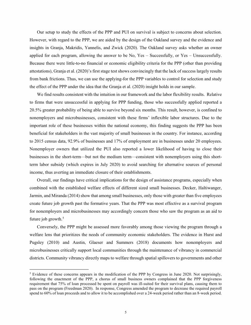
Our empirical contributions emerge out of analyses across four datasets. First are two unique survey

datasets obtained from approximately one thousand small businesses located in Oakland, California.

Second, we hand-collected a dataset of Oakland small business responses to the shelter-in-place order,

codifying which businesses remained fully open, scaled down to a reduced or variant revenue model,

temporarily closed, and permanently closed as of the last week of April, 2020. Third, we use foot traffic

data from SafeGraph, covering consumer visitation data from mobile devices. Finally, we use labor data

for small businesses obtained from HomeBase.

Our first analyses test revenue resiliency by firm size. Within the Oakland survey, businesses across

the board reported a dramatic drop in year-over-year revenues for March 2020; however, we find notable

differences based on firm size, even after controlling for revenue relevant characteristics such as location,

whether the business was essential under the shelter-in-place order, industry fixed effects, and year-over-

year revenues for the prior month. Overall, enterprises experienced the largest percentage decline in

revenues, followed by nonemployer firms. Although struggling, microbusinesses fared the best,

experiencing a revenue decline that was roughly 14% lower than that of enterprises. We obtain remarkably

similar results when we use SafeGraph foot traffic data as a measure of revenue-generating patrons. In a

difference-in-difference estimation with firm fixed-effects, we estimate that, relative to January levels,

enterprises and nonemployers experienced a 73.8% and 73.1% drop in foot traffic in the weeks following

the shelter-in-place order. Microbusinesses fared slightly better, experiencing a 68.4% decline, suggesting

again that microbusiness were able to avoid roughly 14% of the drop felt by enterprises.

Our second series of analyses tests whether labor flexibility differs by firm size. Focusing first on the

Oakland survey data, we find that layoffs of full-time workers and part-time workers had elasticities to firm

size (based on pre-crisis employee headcount) of 0.127 and 0.172, respectively, again controlling for

location effects, whether the business was essential under the shelter-in-place order, industry fixed effects,

as well as March revenue losses. Putting these estimates into the context of our stylized example, they

indicate that enterprises laid off approximately 38% of full-time workers and 50% of part-time workers. In

contrast, microbusinesses exhibited roughly half the labor flexibility of enterprises, laying off

approximately 18% and 24% of their full- and part-time workers, respectively.

We supplement these survey estimates of labor flexibility using HomeBase data. In a differences-in-

differences estimation with firm and week fixed effects, we estimate the elasticity of post-crisis employee

counts and payrolls to firms’ pre-crisis employee headcount, controlling for revenue declines. We find

elasticities of post-crisis labor to pre-crisis worker counts ranging from -0.25 to -0.30, nationally and in

Oakland. Translating these findings into our classification of firms, we find that during the pandemic,

enterprises were able to cut back payrolls 55.1 percent, while microbusinesses cut back only 37.1 percent,

or two-thirds the reduction of enterprises.

3

Third, we investigate the role of committed costs in a firm’s survival across different sized firms. We

base our estimates on respondent’s self-reported probability of having to close permanently, taking residual

closure variation as a proxy for committed costs once we level firms on revenue resiliency and labor

flexibility. We find that closure risk is increasing in worker counts. In particular, relative to microbusinesses

and nonemployers, enterprises face a respective 11% and 22% higher closure risk due to committed costs.

These results are consistent with larger small businesses incurring greater committed costs as they expand

operations, but unlike labor, these costs are less flexible, making them a primary source of closure risk for

growth-oriented small businesses.

We then map these findings to the design of small business disaster assistance, both in the context of

COVID-19 and in other periods of local and national macroeconomic distress. Our mapping puts a framing

on a set of simple intuitions. Working capital loan programs to small businesses (such as conventional

disaster loans offered by the Small Business Administration (SBA)) require revenue resilience mechanisms

to be at work, which at least in the short term would be most effective on microbusinesses and then

nonemployers. Conversely, programs offering subsidies to restructure debt, leases, or other committed costs

would be most effective on survival odds for larger enterprises. Lastly, labor cost-oriented grant and subsidy

programs would be most effective for microbusinesses and nonemployers, who cannot depend on labor

flexibility for survival, since the labor force consists of core employees.

Consider, for example, the landmark PPP implemented as part of the Coronavirus Aid, Relief, and

Economic Security (CARES) Act in March 2020. The PPP authorizes the expenditure of nearly $610 billion

in small business loans. As suggested by its name, PPP loans were intended to subsidize labor, and the

original terms of the program provided that loans could be forgiven entirely if a business spends at least

75% of loan proceeds to maintain pre-crisis payrolls in the first eight weeks following loan disbursement.

But given our findings regarding labor flexibility, this subsidy sits uncomfortably with the survival

capabilities of larger enterprises who may have little need for a labor subsidy given their ability to scale

back labor to match reduced revenues. Consistent with this observation, Chetty et al. (2020) find that the

PPP failed to spur employment among businesses receiving a PPP loan. Their sample, however, did not

include microbusinesses, for which a labor subsidy may have been more useful under our framework.

To explore this possibility, we turn to the second Oakland survey—a follow-up survey conducted in

June 2020 that focused specifically on the aid that Oakland small businesses had pursued as well as their

short-term and medium-term projections for survival. Of particular interest is utilization of PPP loans and

the PUI authorized by the CARES Act. Both programs represent a labor subsidy insofar that they were

intended to cover labor costs for employer and nonemployer businesses. As such, they should be especially

useful for those businesses that continue operations but are limited in their ability to scale down labor costs.

4

Our setup to study the effects of the PPP and PUI on survival is subject to concerns about selection.

However, with regard to the PPP, we are aided by the design of the Oakland survey and the evidence and

insights in Granja, Makridis, Yannelis, and Zwick (2020). The Oakland survey asks whether an owner

applied for each program, allowing the answer to be No, Yes – Successfully, or Yes – Unsuccessfully.

Because there were little-to-no financial or economic eligibility criteria for the PPP (other than providing

attestations), Granja et al. (2020)’s first stage test shows convincingly that the lack of success largely results

from bank frictions. Thus, we can use the applying-for the PPP variables to control for selection and study

the effect of the PPP under the idea that the Granja et al. (2020) insight holds in our sample.

We find results consistent with the intuition in our framework and the labor flexibility results. Relative

to firms that were unsuccessful in applying for PPP funding, those who successfully applied reported a

20.5% greater probability of being able to survive beyond six months. This result, however, is confined to

nonemployers and microbusinesses, consistent with these firms’ inflexible labor structures. Due to the

important role of these businesses within the national economy, this finding suggests the PPP has been

beneficial for stakeholders in the vast majority of small businesses in the country. For instance, according

to 2015 census data, 92.9% of businesses and 17% of employment are in businesses under 20 employees.

Nonemployer owners that utilized the PUI also reported a lower likelihood of having to close their

businesses in the short-term—but not the medium term—consistent with nonemployers using this short-

term labor subsidy (which expires in July 2020) to avoid searching for alternative sources of personal

income, thus averting an immediate closure of their establishments.

Overall, our findings have critical implications for the design of assistance programs, especially when

combined with the established welfare effects of different sized small businesses. Decker, Haltiwanger,

Jarmin, and Miranda (2014) show that among small businesses, only those with greater than five employees

create future job growth past the formative years. That the PPP was most effective as a survival program

for nonemployers and microbusinesses may accordingly concern those who saw the program as an aid to

future job growth.5

Conversely, the PPP might be assessed more favorably among those viewing the program through a

welfare lens that prioritizes the needs of community economic stakeholders. The evidence in Hurst and

Pugsley (2010) and Austin, Glaeser and Summers (2018) documents how nonemployers and

microbusinesses critically support local communities through the maintenance of vibrancy in commercial

districts. Community vibrancy directly maps to welfare through spatial spillovers to governments and other

5 Evidence of these concerns appears in the modification of the PPP by Congress in June 2020. Not surprisingly, following the enactment of the PPP, a chorus of small business owners complained that the PPP forgiveness requirement that 75% of loan processed be spent on payroll was ill-suited for their survival plans, causing them to pass on the program (Freedman 2020). In response, Congress amended the program to decrease the required payroll spend to 60% of loan proceeds and to allow it to be accomplished over a 24-week period rather than an 8-week period.

5

community stakeholders through commercial and residential property tax bases (Alm, Buschman, and

Sjoqvist, 2014; Shoag and Veuger, 2018; Tsivanidis and Gechter, 2019) and through support for females

and minority entrepreneurship (SBA, 2018). Thus, taken in this light, the proportion of PPP funds tapped

by microbusinesses and nonemployers might have induced large welfare gains. Such a finding would

provide a counterpoint to prominent arguments for letting existing unemployment insurance nets and

creative destruction work in the market in an effort to save funds for the revival of growing enterprises,

rather than subsidizing survival of all small businesses (Rajan, 2020). In short, designing small business

assistance with a single-minded focus on job creation risks creating zombie main streets and a greater

geographic concentration of commerce and wealth (Austin, Glaeser and Summers, 2018).

To make more progress on these welfare tradeoffs is beyond the scope herein. Yet, sound small business

policy points to the need to account for the divergent welfare effects of supporting different size small

businesses through periods of macro distress. For the same reasons, policy must also consider how the

heterogeneities in small business survival capabilities map to the design of specific small business

assistance programs. Our contribution is to provide that mapping.

The rest of the paper is organized as follows. In Section 2 we present our framework for small business

survival capabilities. We describe our data in Section 3 and provide summary statistics for each of the four

data sets that comprise it. Our empirical results are reported in Section 4. Section 5 examines the policy

implications of our findings with respect to the design of small business assistance programs. Section 6

reports on whether the PPP and PUI affect medium term survival in Oakland, building off the policy frame.

Section 7 concludes.

2. FRAME

We lay out a simple frame of the components of firm-level cash flows to fix ideas. We define cash

flows π as net revenues (𝑟𝑟) minus labor costs (𝑙𝑙) and committed other costs (𝑐𝑐):

π = 𝑟𝑟 − 𝑙𝑙 − 𝑐𝑐, (1)

where net revenues (𝑟𝑟) is revenues minus the inventory costs of goods sold. We consider a negative macro

shock 𝑅𝑅− to the economy, which imposes a loss of a unit of net revenue on average for small businesses,

but with variance across firms. We are interested in the survival of a firm defined as the maintenance of

positive cash flows from the existing cash flow position of the firm following the macro shock, or:

𝑠𝑠𝑠𝑠𝑟𝑟𝑠𝑠𝑠𝑠𝑠𝑠𝑠𝑠𝑙𝑙 ∶= π + 𝑑𝑑π𝑑𝑑𝑅𝑅−

> 0. (2)

Taking the derivative and allowing for labor to scale with revenues or be directly impacted by the shock,

we have the survival condition as:

6

�𝑟𝑟 + 𝑑𝑑r𝑑𝑑𝑅𝑅−

��������𝑟𝑟𝑟𝑟𝑟𝑟𝑟𝑟𝑟𝑟𝑟𝑟𝑟𝑟 𝑔𝑔𝑟𝑟𝑔𝑔𝑔𝑔

− �𝑙𝑙 + 𝜕𝜕𝑙𝑙𝜕𝜕𝑟𝑟

𝑑𝑑𝑟𝑟𝑑𝑑𝑅𝑅−

+ 𝑑𝑑𝑙𝑙𝑑𝑑𝑅𝑅−

��������������𝑙𝑙𝑙𝑙𝑙𝑙𝑙𝑙𝑟𝑟 𝑓𝑓𝑙𝑙𝑟𝑟𝑓𝑓𝑔𝑔𝑙𝑙𝑔𝑔𝑙𝑙𝑔𝑔𝑔𝑔𝑓𝑓

− �𝑐𝑐 + 𝑑𝑑c𝑑𝑑𝑅𝑅−

��������

𝑐𝑐𝑙𝑙𝑐𝑐𝑐𝑐𝑔𝑔𝑔𝑔𝑔𝑔𝑟𝑟𝑑𝑑 𝑐𝑐𝑙𝑙𝑐𝑐𝑔𝑔𝑐𝑐

> 0.

(3)

Survival is a function, first, of the ability of firms to exhibit revenue resiliency, preserving as much of ex

ante revenue as possible. Next, survival is a function of labor cost flexibility, which incorporates how elastic

a firm’s labor cost is to revenue as well as direct labor effects from the macro shock. Finally, survival is a

function of the size of the committed costs and the ability to restructure costs following the shock 𝑅𝑅−.

In our empirical analysis, we assume that the ability to deploy these three survival tactics are capabilities

of firms in the sense that firms will optimally do whatever they can to adjust to the macro shock. We

estimate these survival capabilities with the lens of looking at how they vary by firm size, focusing on our

three categories of nonemployers, microbusinesses, and enterprises, all within industry sector.

We then map the results to inferences concerning policies aimed at supporting small businesses during

periods of macro distress. In particular, we consider three sets of program features in terms of how they

relate to our frame:

Subsidized Working Capital Loans. Programs such as Economic Injury Disaster Loans (EIDL)

offered through the SBA provide subsidized loans to business struggling with natural disasters.

These programs impose conditions on recipients to ensure that loan proceeds are used to support

working capital in rebuilding revenues. Recipients of EIDLs, for instance, are prohibited from using

loan proceeds to refinance long-term debt or expand operations. As summarized by the SBA,

EIDLs are for entities who are “ready to ‘restart’ their operations once circumstances allow” (SBA

2020). These subsidized working capital loans should therefore be most useful for those firms that

have revenue resiliency among their survival capabilities.

Labor Costs Grants and Subsidies. Programs such as the Paycheck Protection Program and

Pandemic Unemployment Insurance (as used by nonemployers as income-substitution) provide a

subsidy to labor costs, conditional on labor remaining in place. Payroll tax holidays (e.g., on the

employer match for Social Security payroll taxes, as was done by President Carter in Jobs Tax

Credit in the Tax Reduction and Simplification Act of 1977 and more recently in the CARES Act)

would also subsidize continuing employment. These policies will be effective when most workers

are either the owner or core function employees, but may be less efficient and attractive for small

businesses endowed with high labor flexibility that they use to survive business cycle downturns.

Lease or Debt Payment Restructuring Subsidies. Governments might choose to implement policies

aimed to reduce the committed cost burdens on small businesses akin to the Home Affordable

7

Modification Program (HAMP) applied to households and lenders during the Great Recession

whereby the government subsidizes the lender (or leaseholder) to restructure the obligation. In the

context of small businesses, these programs may take the form of providing government grants that

can be used to offset commercial lease costs. Facilitating small businesses bankruptcy

reorganizations would also have the effect of providing small businesses with leverage to

restructure large committed costs. We provide examples of both forms of these programs in Section

5. Either form of program will be especially relevant for small businesses whose survival will

depend on their ability to restructure large committed costs incurred prior to the macro shock.

3. DATA AND SUMMARY STATISTICS

A primary challenge confronting research about small businesses concerns the unavailability of firm

performance data. We address this challenge through a multi-step data collection process that exploits our

ability to collect real-time data as small businesses began to experience the impact of the COVID-19

economic shutdown. These real-time data come from the following four sources.

A. City of Oakland Small Business Survey

In early March 2020, well before Alameda County imposed its shelter-in-place order, the City of

Oakland constructed a survey to elicit information from its small business community about resiliency

during the COVID-19 pandemic. The City’s survey went live three days prior to the March 16th

announcement of the County’s shelter-in-place. Our core analyses focus on responses submitted between

March 13, 2020 through April 1, 2020. Our sample starts with 1,088 surveys. After filtering out 37

businesses with more than 50 employees, 19 purely online businesses, and 18 nonprofits, we have a sample

of 1,014 firms. Based on census data, we estimate that the survey captured approximately 11-15% percent

of the city’s businesses.6

Table 1 reports the summary statistics from the City of Oakland survey. Panel A reports the sample

statistics regarding employment, covering the following variables:

⋅ Nonemployer : = An indicator for the firm reporting no employees.

⋅ Microbusiness: = An indicator for the firm reporting 1-5 employees.

⋅ Enterprise : = An indicator for the firm reporting 6-50 employees.

6 According to the 2017 County Business Patterns from the U.S. Census Bureau, there were nearly 14,000 private and government establishments in Oakland’s zip codes. Using this number directly would imply that our sample captures 7.8% of Oakland’s businesses, but this is too conservative as the census total (i) includes businesses with up to 500 employees (and our survey is for small businesses), (ii) assumes that small businesses only have one establishment, (iii) includes non-revenue generating registered businesses, and (iv) includes schools, government offices, and other non-business organizations.

8

⋅ Employees : = Full-time and part-time employees prior to March, 2020.

⋅ Percentage Change Job Losses : = Full-time and part-time positions lost early in the

shutdown, relative to reported pre-crisis full- and part-time positions.

A quarter of the sample of Oakland small business are nonemployers, 43% are microbusinesses, and 32%

are enterprises. The mean (median) employee count is 6.5 (2) for all small businesses and 8.7 (4) for

businesses excluding the nonemployers. Of these jobs, 17.7% were already lost on average in the first weeks

of the shelter-in-place.

Panel B reports statistics on reported revenues.

⋅ Declining : = Whether or not the business was ex ante declining, defined as year-over-year

declining in gross receipts as of February 2020.

⋅ Percentage Change Receipts : = Reported percentage change year-over-year gross receipts

as of March 2020 based on a firm’s selection of one of six ranges.

Approximately half of all respondents indicated a decline in year-over-year (YoY) revenue as of

February 2020, the month prior to the shelter-in-place order. We use this indicator variable below as our

proxy for indicating whether a firm’s financial distress pre-dated the U.S. COVID-19 crisis. The fact that

half of small businesses might have negative growth is consistent with the results in Decker et al. (2014)

and Hurst and Pugsley (2011) concerning the non-growth nature of most small businesses. Also in Panel

B, we report the distribution of gross receipts YoY as of March 2020. By early March, businesses were

severely impacted first by self-imposed staying out of public spaces and then, on March 16, by the county

ordinance. This shows up in the distribution in Panel B, where 69% of respondents report a year-over-year

decline of over 40% for March.

In Panel C, we report the distribution to the response on closure risk.

⋅ Closure Risk : = Whether the small business owner responded that s/he was “very

concerned” about the risk of closure, “somewhat concerned” or “not concerned”.

Overall, 73% of respondents were very concerned about closure and only 4%, not concerned.

As part of this survey, the City of Oakland subsequently conducted a follow-up survey completed by

nearly 300 of the small businesses. We examine this follow-up survey in Section 5.

B. Hand Collected Information on Small Business Operations

We obtain additional operating data on these businesses from manual firm-by-firm internet searches

conducted between April 24, 2020 and May 3, 2020—the day on which Alameda County permitted certain

outdoor businesses to recommence operations on a limited basis. We began these manual searches on

Google Maps. Companies, particularly street-facing companies, had a large incentive to keep their Google

Maps status updated, and businesses informed us that Google aggressively solicited each establishment for

9

this information. We additionally searched for the company website and other internet sources of

information to determine the operating status for each survey company.

For each business, we coded the following variables.

⋅ Industry ∶= Narrowly-defined industry.

⋅ Main Street : = An indicator for a business being on a street-facing location (on “main street”).

⋅ Essential : = Whether the business constitutes an “essential business” under Alameda County’s

shelter-in-place order (e.g., grocery stories, lumber and repair, pharmacies, and physician

offices).

Panel A of Table 2 breaks down the distribution of industries and provides detailed examples of the type of

businesses in each category. Panel B reports that two-thirds of the sample are “main street” facing, and a

third provide their goods and services at a home or at an office that is not “main street” facing. We coded

eleven percent of respondents to be deemed essential businesses under the shelter-in-place rules.

Panel C of Table 2 reports the status of the ongoing concern.

⋅ Status : = The hand-coded operating status of the business at the time of the search, coded

among: Permanently Closed (or Lacking Ongoing Concern Signal), Temporarily Closed,

Trying, and Open.

A firm classified as Trying (21%) indicates a firm that was not permitted to operate under the shelter-in-

place order but nevertheless conducted operations under alternative arrangements or reduced revenue

models. For example, this class of businesses might include a restaurant that operated on a limited take-

out/delivery basis or a yoga studio that operated remotely through video conferencing. The Temporarily

Closed status, which was actively pursued by Google Maps to provide its customers with accurate

availability of businesses, accounted for approximately 26% of the sample. We overrode Google Map’s

Temporarily Closed to be Trying if the business website indicated that it was operating in some form to

generate revenues; most Trying businesses were marked Temporarily Closed by Google, except for

restaurants, which were market “take-out only” or “delivery only” (or both). The Permanently Closed (or

Lacking Ongoing Concern Signal) businesses (19%) were a combination of those businesses that were

explicitly marked as permanently closed by Google Maps as well as those businesses which showed no

sign of any ongoing business on their webpages and did not indicate that they were temporarily closed.

In Figure 1, we plot the status by industry in pie charts, to underscore the economic challenge to survey

respondents posed by the COVID-19 pandemic. Temporary closures were especially high within the salons,

retail, fitness/salon/wellness sector, and construction sectors. Only in the medical, professional services and

personal services was the Open category the dominant classification. In contrast, the Trying classification

was prevalent among restaurants, fitness, and retail.

10

C. HomeBase

Our third set of data comes from HomeBase, a workplace scheduling and payroll management company

that caters primarily to small businesses.7 The HomeBase data includes anonymized data for an

establishment’s weekly employee headcount and, for some firms, reported weekly wages paid to some or

all employees. We filter the HomeBase data to all business establishments that have a U.S. zip code and a

disclosed industry and that have 50 or fewer average employees between January 1, 2020 and February 15,

2020.

In Panel A of Table 3 we report summary statistics for this sample of HomeBase establishments. Our

primary interest is in the following two weekly measures:

⋅ Headcount : = Weekly full- and part-time employees (regardless of whether wages are

disclosed) per location.

⋅ Payroll : = Weekly wages paid to employees for whom wages are disclosed.

Column 1 – 4 indicate that HomeBase firms within our sample had a mean (median) employee headcount

of 7.6 (5.5) during the period January 1, 2020 and February 15, 2020. Not surprisingly, employee headcount

varied by industry, ranging from a low of 4.34 (3) among establishments in the Beauty & Personal Care

industry to a high of 9.21 (7.3) within the Food & Drink industry. In Columns 5 – 8 we similarly present

summary data concerning total weekly wages paid for those establishments that reported the weekly wages

paid to one or more employees over the same period. Among these firms, mean (median) pre-crisis wages

paid per week were roughly $2,400 ($1,500). Across industries, Beauty & Personal Care establishments

were the lowest paying within the sample, while Transportation establishments paid the most, presumably

reflecting the higher hourly wage rates paid by these latter firms.

In Figure 2 we plot the distribution of our sample of HomeBase establishments by state. California,

Florida and Texas claim roughly 16%, 10, and 9% of establishments, respectively.

D. SafeGraph Foot Traffic Data

Our final dataset is data on foot traffic in establishments from SafeGraph for January 1, 2020 to April

30, 2020. SafeGraph covers mobile locations for over thirty million individuals using cellphone tracking

information that these individuals have consented to sharing pursuant to one or more applications installed

on their mobile devices. SafeGraph overlays this tracking data to 5 million U.S. establishments or “points

of interest” (POI) based on the actual location and shape of the POI (i.e., its polygon) rather than its address,

thus allowing SafeGraph to identify each instance when an individual visits a POI.

7 These data have been made available by HomeBase for researchers examining the labor market impact of COVID-19 and have been a primary source of data for examining overall employment trends within the small business sector during the COVID-19 economic crisis (see, e.g., Bartik, et al.).

11

Figure 3 maps the mean number of devices during this period for all counties in the continental U.S.

and within California. SafeGraph tracked over one thousand devices in over half of all counties. In Alameda

county, the focus of our study, SafeGraph tracked over 50,000 devices, allowing us to use these data as a

proxy for the revenue of small businesses, particularly for “main street” businesses whose cash flow is

likely to depend on foot traffic.

We cannot use the data to infer dollars of revenue per se, as different store types have different

conversion rates of customers to revenues. Yet, we can use foot traffic to infer the revenue shock, using

firm fixed effects, following the approach of investigative journalists and policymakers examining the

impact of the COVID-19 crisis on consumers.8 Figure 4 illustrates the feasibility of this approach, focusing

on select industries within Alameda—Restaurants, Electronics and Appliance Stores, Fitness/Sports

Centers, and Grocery Stores. We standardize visits by observed daily devices and calculate the moving

average over the preceding seven-day period. Plotted is the moving average over time relative to that for

January 8, 2020. All businesses suffered a significant drop in foot traffic following the shelter in place

order, which is represented by the dashed vertical line on March 16. The primary exception relates to the

surge in grocery store foot traffic in the days immediately following the announcement of the order as

residents flooded grocery stores.

We match the Oakland small businesses survey respondents to the Safe Graph POI dataset by business

name, enabling us to assess directly the extent to which a business’ foot traffic was impacted by Alameda

County’s shut-down in economic activity. (Service companies without storefronts – construction,

consulting, realty, etc. – are often not covered in SafeGraph, nor would foot traffic represent a meaningful

concept of commerce for these businesses.) These foot traffic data span from January 1, 2020 to April 30,

2020; however, we drop the period of closing down in late March (March 16 to March 31), to ensure that

our foot traffic data reflects commercial activity as opposed to visits related to the closing down of a

business. We find exact matches for 268 small businesses, mostly for main street-facing businesses.

We report in Panel B of Table 3 summary statistics for our primary metric of interest, average daily

foot traffic for each location by coded industry. As in Figure 4, the reported figures account for variation in

the number of observed devices by scaling the daily visits to an observed POI by the number of devices

observed by SafeGraph in Alameda County per 100,000 residents. Data represent the overall mean number

of standardized daily visits between January 1, 2020 and March 15, 2020. Across industries, this

standardized measure of daily visits ranged from a mean (median) of 0.85 (0.74) for medical offices to 7.55

(5.37) for restaurants.

8 See, e.g., Megan Cerullo, Phone data show consumers avoiding stores, restaurants as COVID surges, CBS News, July 2, 2020, available at https://www.cbsnews.com/news/cell-phone-data-show-consumers-avoiding-stores-as-covid-19-cases-surge/.

12

4. RESULTS

We test whether the facets of small business survival – revenue resiliency, labor flexibility, and

committed cost – vary by firm size in their reaction to the economic crisis caused by the COVID-19 shelters-

in-place. In our estimations, we consider the role of ex ante (pre-crisis) firm size using two independent

variables – the natural log of workers (where “workers” equals employees + 1, the owner) and an indicator

for a nonemployer firm. The nonemployer indicator is used to pick up any unique attributes of

nonemployers that a continuous variable might miss. We then group predictions into three size buckets

(following our bakery, taqueria, and pizza restaurant examples) to depict patterns of the predicted effects

by size type, always absorbing industry or firm fixed effects, to depict patterns orthogonal to these

systematic influences.

A. Revenue Resilience Results

A.1. Oakland Survey Revenue Resilience Results

Table 4 presents results from two revenue resiliency analyses. In column 1-4, we report estimates within

the Oakland survey data as follows, denoting the small business by i:

𝐿𝐿𝐿𝐿𝐿𝐿(% △ 𝑅𝑅𝑅𝑅𝑐𝑐𝑅𝑅𝑠𝑠𝑅𝑅𝑅𝑅𝑠𝑠 𝐷𝐷𝑅𝑅𝑐𝑐𝑙𝑙𝑠𝑠𝐷𝐷𝑅𝑅 𝑀𝑀𝑠𝑠𝑟𝑟𝑐𝑐ℎ)𝑔𝑔 = 𝛽𝛽0 + 𝛽𝛽1𝐿𝐿𝐿𝐿𝐿𝐿𝐿𝐿𝐿𝐿𝑟𝑟𝐿𝐿𝑅𝑅𝑟𝑟𝑠𝑠𝑔𝑔𝑃𝑃𝑟𝑟𝑟𝑟 + 𝛽𝛽2𝑁𝑁𝐿𝐿𝐷𝐷𝑅𝑅𝑁𝑁𝑅𝑅𝑙𝑙𝐿𝐿𝑁𝑁𝑅𝑅𝑟𝑟𝑔𝑔

+ 𝛽𝛽3𝐿𝐿𝐿𝐿𝐿𝐿(% △ 𝑅𝑅𝑅𝑅𝑐𝑐𝑅𝑅𝑠𝑠𝑅𝑅𝑅𝑅𝑠𝑠 𝐷𝐷𝑅𝑅𝑐𝑐𝑙𝑙𝑠𝑠𝐷𝐷𝑅𝑅 𝐹𝐹𝑅𝑅𝐹𝐹𝑟𝑟𝑠𝑠𝑠𝑠𝑟𝑟𝑁𝑁)𝑔𝑔 + 𝜇𝜇𝑐𝑐𝑙𝑙𝑔𝑔𝑟𝑟𝑐𝑐𝑔𝑔𝑟𝑟𝑟𝑟𝑟𝑟𝑔𝑔 + 𝜇𝜇𝑟𝑟𝑐𝑐𝑐𝑐𝑟𝑟𝑟𝑟𝑔𝑔𝑔𝑔𝑙𝑙𝑙𝑙

+ 𝜇𝜇𝑔𝑔𝑟𝑟𝑑𝑑𝑟𝑟𝑐𝑐𝑔𝑔𝑟𝑟𝑓𝑓 + 𝜀𝜀𝑔𝑔

(4)

The dependent variable is the log of 1 plus the percentage change decline in YoY gross receipts for March

2020.9 The dependent variable is increasing in the decline in revenues. All columns include the variable

%Δ R𝑅𝑅𝑐𝑐𝑅𝑅𝑠𝑠𝑅𝑅𝑅𝑅𝑠𝑠 𝐷𝐷𝑅𝑅𝑐𝑐𝑙𝑙𝑠𝑠𝐷𝐷𝑅𝑅 𝐹𝐹𝑅𝑅𝐹𝐹𝑟𝑟𝑠𝑠𝑠𝑠𝑟𝑟𝑁𝑁, which is the same variable as the dependent variable except YoY

revenue is reported as of February, 2020, thus allowing us to parse-out the pre-crisis situation of the firm

and focus on the effect of the pandemic stress. In addition, all columns include indicators for the business

being located on main street (𝜇𝜇𝑐𝑐𝑙𝑙𝑔𝑔𝑟𝑟𝑐𝑐𝑔𝑔𝑟𝑟𝑟𝑟𝑟𝑟𝑔𝑔) and whether or not the business is essential (𝜇𝜇𝑟𝑟𝑐𝑐𝑐𝑐𝑟𝑟𝑟𝑟𝑔𝑔𝑔𝑔𝑙𝑙𝑙𝑙). All

columns have our main independent variable, log of workers, and Columns 2 and 4 also include the

nonemployer indicator to allow for any unique attributes of this type of business. Columns 3 and 4 include

industry fixed effects (𝜇𝜇𝑔𝑔𝑟𝑟𝑑𝑑𝑟𝑟𝑐𝑐𝑔𝑔𝑟𝑟𝑓𝑓).

Turning to the results, we first look to the conditioning variable Log Receipts Decline February. The

March decline in receipts has a very tightly-estimated elasticity of 0.220 to the February decline in receipts.

This elasticity is well below 1, reflecting the large change in the setting in March. Nevertheless, this variable

9 Note that the gross receipt decline variables are reported in the survey in buckets, as depicted in Table 1, not as a continuous variable. We make a continuous variable, taking the midpoint of the bucket as the value. An ordinal logit estimation fits a similar pattern as what we report, but with more noise.

13

is the most important in terms of partial R-squared in the estimation, even much more so than the industry

effects, which are surprisingly insignificant with other variables included. The main street and essential

variables (which sometimes compete with the industry effect for power) are also weak in explanatory

power. In short, it appears that the shelter-in-place affected businesses across the board, hitting those

already in decline 22% more, but with much idiosyncratic impact.

Our main variables of interest, workers and nonemployers, are also statistically important. We find a

gross receipts elasticity of 0.027 to the number of workers in the firm, once we allow nonemployer firms

to exhibit their own pattern (columns 2 and 4). Larger firms exhibit a greater percentage revenue decline.

In Figure 5, panel A, we plot the marginal effect of log workers and nonemployer status on percentage

decline in gross receipts for March at the mean value of all other variables (using the specification shown

in column 4.) We plot this marginal effect averaged into our three small business types – nonemployers,

microbusiness, and enterprises. The figure shows that microbusinesses face a YoY revenue percentage

decline for March of -0.408, a large number, but better than enterprises, who face a revenue decline of -

0.476 as a percent of the prior year’s gross receipts. Interpreting the result in the context of our setup,

microbusinesses seem to be endowed with the ability to ward off 14% of the shock relative to enterprises.

In the context of real-world events captured by our hypothetical businesses, the taqueria—because it is

small—is able to more nimbly keep a larger proportion of pre-crisis revenues.

A.2. SafeGraph Revenue Resilience Results

In the last two columns of Table 4, we instead turn to the SafeGraph data of foot traffic as a revenue

proxy, again focusing on Oakland, where we know employee counts. These data are a panel, allowing us

to estimate a model to absorb firm heterogeneity and time, akin to a difference in differences model, but

against the continuous variable 𝐿𝐿𝐿𝐿𝐿𝐿𝐿𝐿𝐿𝐿𝑟𝑟𝐿𝐿𝑅𝑅𝑟𝑟𝑠𝑠𝑔𝑔𝑃𝑃𝑟𝑟𝑟𝑟.

𝐿𝐿𝐿𝐿𝐿𝐿𝐹𝐹𝐿𝐿𝐿𝐿𝑅𝑅𝐹𝐹𝑟𝑟𝑠𝑠𝐹𝐹𝐹𝐹𝑠𝑠𝑐𝑐𝑔𝑔𝑔𝑔 = 𝛽𝛽0 ∗ 𝑃𝑃𝐿𝐿𝑠𝑠𝑅𝑅𝑔𝑔 + 𝛽𝛽1𝐿𝐿𝐿𝐿𝐿𝐿𝐿𝐿𝐿𝐿𝑟𝑟𝐿𝐿𝑅𝑅𝑟𝑟𝑠𝑠𝑔𝑔𝑃𝑃𝑟𝑟𝑟𝑟𝑃𝑃𝐿𝐿𝑠𝑠𝑅𝑅𝑔𝑔 + 𝛽𝛽2𝑁𝑁𝐿𝐿𝐷𝐷𝑅𝑅𝑁𝑁𝑅𝑅𝑙𝑙𝐿𝐿𝑁𝑁𝑅𝑅𝑟𝑟𝑔𝑔𝑃𝑃𝐿𝐿𝑠𝑠𝑅𝑅𝑔𝑔+ 𝛾𝛾𝑔𝑔 + 𝛿𝛿𝑔𝑔 + 𝜀𝜀𝑔𝑔𝑔𝑔 .

(5)

Variables 𝛾𝛾𝑔𝑔 and 𝛿𝛿𝑔𝑔 denote firm and day fixed effects, respectively. 𝑃𝑃𝐿𝐿𝑠𝑠𝑅𝑅𝑔𝑔 represents March 30 – April 30,

2020.

As shown in columns 5-6 of Table 4, foot traffic fell dramatically across firms during the Post period,

as would be expected. We find that this decline is especially pronounced for nonemployers and larger

businesses. We again turn to a graphical representation to put our economic magnitudes into perspective.

Panel B of Figure 5 plots the predicted log of foot traffic over time by small business type, after

removing firm fixed effects. Note that for the pre-crisis period, the lines pick up a single time-varying

pattern because LogWorkers is static by firm (and thus absorbed by the fixed effect) until March 30, when

the interaction with Post estimates elasticities by firm size. As the picture illustrates, all types of businesses

14

incurred a tremendous reduction in foot traffic after the shelter-in-place order; the average decline is 71.9%.

However, whereas enterprises and nonemployers face 73.8% and 73.1% percentage declines in their foot

traffic, microbusinesses have somewhat higher revenue resiliency, facing only a 68.4% decline. This is not

to say that a 68% decline in revenues is benign, but microbusinesses seem to be able to ward off 8% of the

shock relative to the other types of business, on the order (14% better) of our finding in the Oakland survey.

B. Labor Flexibility Results

In the forthcoming labor flexibility and committed costs estimations, we need to control for revenue

losses, to avoid double-counting any effects we estimate in Table 4 by firm size. Thus, we create a revenue

loss index variable, defined as the average of a standardized version of the percentage decline in revenue

for March from the Oakland survey and a standardized version of the percentage change in foot traffic after

the shelter in place (defined to be April) relative to the pre-period foot traffic of January 13 – February 18,

2020. Because some observations lack one or the other variable, we allow solo contributions of these

standardized variables.

B.1. Oakland Survey Labor Flexibility Results

We now test whether the labor flexibility facet of small business survival varies by firm size in its

reaction to the economic crisis caused by the pandemic. Table 5 presents estimates of labor flexibility in

the Oakland survey in the following specification:

𝐹𝐹𝑟𝑟𝑠𝑠𝑐𝑐𝑅𝑅𝑠𝑠𝐿𝐿𝐷𝐷𝑠𝑠𝑙𝑙𝐿𝐿𝐿𝐿𝐿𝐿𝑠𝑠𝑅𝑅( % △ 𝐷𝐷𝑅𝑅𝑐𝑐𝑙𝑙𝑠𝑠𝐷𝐷𝑅𝑅 𝐿𝐿𝐿𝐿𝑟𝑟𝐿𝐿𝑅𝑅𝑟𝑟𝑠𝑠𝑔𝑔) = 𝛽𝛽1𝐿𝐿𝐿𝐿𝐿𝐿𝐿𝐿𝐿𝐿𝑟𝑟𝐿𝐿𝑅𝑅𝑟𝑟𝑠𝑠𝑔𝑔𝑃𝑃𝑟𝑟𝑟𝑟

+ 𝛽𝛽2𝑅𝑅𝑅𝑅𝑠𝑠𝐿𝐿𝐿𝐿𝑠𝑠𝑠𝑠𝑅𝑅𝐷𝐷𝑅𝑅𝑅𝑅𝑅𝑅𝑔𝑔 + 𝛽𝛽3𝐿𝐿𝐿𝐿𝐿𝐿𝐿𝐿𝐿𝐿𝑟𝑟𝐿𝐿𝑅𝑅𝑟𝑟𝑠𝑠𝑔𝑔𝑃𝑃𝑟𝑟𝑟𝑟𝑅𝑅𝑅𝑅𝑠𝑠𝐿𝐿𝐿𝐿𝑠𝑠𝑠𝑠𝑅𝑅𝐷𝐷𝑅𝑅𝑅𝑅𝑅𝑅𝑔𝑔 + 𝜇𝜇𝑐𝑐𝑙𝑙𝑔𝑔𝑟𝑟𝑐𝑐𝑔𝑔𝑟𝑟𝑟𝑟𝑟𝑟𝑔𝑔

+ 𝜇𝜇𝑟𝑟𝑐𝑐𝑐𝑐𝑟𝑟𝑟𝑟𝑔𝑔𝑔𝑔𝑙𝑙𝑙𝑙 + 𝜇𝜇𝑔𝑔𝑟𝑟𝑑𝑑𝑟𝑟𝑐𝑐𝑔𝑔𝑟𝑟𝑓𝑓 + 𝜀𝜀𝑔𝑔.

(6)

The dependent variable is a percentage change decline of workers (full-time in columns 1-3 and part-time

in columns 4-6). The main independent variable is 𝐿𝐿𝐿𝐿𝐿𝐿𝐿𝐿𝐿𝐿𝑟𝑟𝐿𝐿𝑅𝑅𝑟𝑟𝑠𝑠𝑔𝑔𝑃𝑃𝑟𝑟𝑟𝑟. Because the percentage change

decline distribution ranges from 0 to 1, we estimate a fractional logit for efficiency. As before, we control

for the main street and essential business effects and absorb industry effects. We include the revenue loss

index to control for the effects documented in Table 4. We also interact the revenue loss index with

𝐿𝐿𝐿𝐿𝐿𝐿𝐿𝐿𝐿𝐿𝑟𝑟𝐿𝐿𝑅𝑅𝑟𝑟𝑠𝑠𝑔𝑔𝑃𝑃𝑟𝑟𝑟𝑟 in some specifications to test whether firm size alters the relationship between labor

flexibility and revenues. We focus our analysis on microbusinesses and small enterprises, since

nonemployers have no employees.

As Table 5 reports, we find that layoffs of full-time workers (columns 1-3) exhibit an elasticity to firm

size of 0.127, controlling for industry effects (column 2), and layoffs of part-time workers (columns 4-6)

exhibit an elasticity 0.172 (column 5) to firm size with these controls. A second result in Table 5 is that

although the relationship between revenue losses and labor layoffs is high, as one would expect, the

15

interaction of revenue loss and pre-crisis level of workers does not add to the explanatory power. Thus,

labor flexibility does not appear to be mediated through differentials in revenue losses among enterprises

relative to microbusinesses.

As before, we turn to a figure to depict the economic meaning of our results. Figure 6, panel A plots

the relationship between ex ante size of the firm and the marginal effect of the 𝐿𝐿𝐿𝐿𝐿𝐿𝐿𝐿𝐿𝐿𝑟𝑟𝐿𝐿𝑅𝑅𝑟𝑟𝑠𝑠𝑔𝑔𝑃𝑃𝑟𝑟𝑟𝑟 on layoffs,

taking all other variables at the mean value. For full-time workers, enterprises on average laid off 38.1

percent of workers, whereas microbusinesses only laid off 17.7 percent. For part-time workers, enterprises

laid off 49.6 percent of workers and microbusinesses only 23.8 percent. Recalling that the ability to lay off

employees to downsize costs can represent a positive aspect for survival, this result implies that

microbusinesses face a much larger risk of not surviving on this metric. In particular, microbusinesses

exhibit half (47.6%) the labor flexibility of enterprises.

B.2. Homebase Labor Flexibility Results

Parallel with the Oakland survey data, we now look at the employment and payroll data from

Homebase. As before, we combine with a revenue loss dataset, in this case, with foot traffic data from

SafeGraph. Establishments in the HomeBase data are anonymized; therefore, we cannot match firm-to-

firm. Instead, we match each HomeBase establishment based on its industry and zip code to SafeGraph foot

traffic data and use the mean weekly foot traffic for SafeGraph POIs within the same industry-zip as a proxy

for revenues. For our measure of firm size, we use a HomeBase establishment’s average headcount data

between January 1, 2020 to February 15, 2020. We focus our labor flexibility estimations excluding

nonemployers.

Denoting index j to indicate industry-zip code of firm i, we estimate parameters from the following:

𝐿𝐿𝐿𝐿𝐿𝐿𝐿𝐿𝑠𝑠𝐹𝐹𝐿𝐿𝑟𝑟𝐿𝐿𝐿𝐿𝑠𝑠𝑅𝑅𝑔𝑔𝑔𝑔 = 𝛽𝛽0𝑃𝑃𝐿𝐿𝑠𝑠𝑅𝑅𝑔𝑔+ 𝛽𝛽1𝐿𝐿𝐿𝐿𝐿𝐿𝐹𝐹𝐿𝐿𝐿𝐿𝑅𝑅𝐹𝐹𝑟𝑟𝑠𝑠𝐹𝐹𝐹𝐹𝑠𝑠𝑐𝑐𝑗𝑗𝑔𝑔 + 𝛽𝛽2𝐿𝐿𝐿𝐿𝐿𝐿𝐹𝐹𝐿𝐿𝐿𝐿𝑅𝑅𝐹𝐹𝑟𝑟𝑠𝑠𝐹𝐹𝐹𝐹𝑠𝑠𝑐𝑐𝑗𝑗𝑔𝑔𝑃𝑃𝐿𝐿𝑠𝑠𝑅𝑅𝑔𝑔

+ 𝛽𝛽3𝐿𝐿𝐿𝐿𝐿𝐿𝐿𝐿𝐿𝐿𝑟𝑟𝐿𝐿𝑅𝑅𝑟𝑟𝑠𝑠𝑔𝑔𝑃𝑃𝑟𝑟𝑟𝑟𝑃𝑃𝐿𝐿𝑠𝑠𝑅𝑅𝑔𝑔 + 𝛽𝛽4𝐿𝐿𝐿𝐿𝐿𝐿𝐿𝐿𝐿𝐿𝑟𝑟𝐿𝐿𝑅𝑅𝑟𝑟𝑠𝑠𝑔𝑔𝑃𝑃𝑟𝑟𝑟𝑟𝐿𝐿𝐿𝐿𝐿𝐿𝐹𝐹𝐿𝐿𝐿𝐿𝑅𝑅𝐹𝐹𝑟𝑟𝑠𝑠𝐹𝐹𝐹𝐹𝑠𝑠𝑐𝑐𝑗𝑗𝑔𝑔

+ 𝛽𝛽5𝐿𝐿𝐿𝐿𝐿𝐿𝐿𝐿𝐿𝐿𝑟𝑟𝐿𝐿𝑅𝑅𝑟𝑟𝑠𝑠𝑔𝑔𝑃𝑃𝑟𝑟𝑟𝑟𝐿𝐿𝐿𝐿𝐿𝐿𝐹𝐹𝐿𝐿𝐿𝐿𝑅𝑅𝐹𝐹𝑟𝑟𝑠𝑠𝐹𝐹𝐹𝐹𝑠𝑠𝑐𝑐𝑗𝑗𝑔𝑔𝑃𝑃𝐿𝐿𝑠𝑠𝑅𝑅𝑔𝑔 + 𝛾𝛾𝑔𝑔 + 𝛿𝛿𝑔𝑔 + 𝜀𝜀𝑔𝑔𝑔𝑔 ,

(7)

where the labor cost dependent variable is either workers or payroll. Variables 𝛾𝛾𝑔𝑔 and 𝛿𝛿𝑔𝑔 denote firm and

week fixed effects, respectively. 𝑃𝑃𝐿𝐿𝑠𝑠𝑅𝑅𝑔𝑔 represents the weeks commencing March 15 – April 19, 2020.

Results are presented in Table 6, first for the area surrounding Oakland (the 94XXX zip codes, including

the East Bay, North Bay and San Francisco) in columns 1-3 and then nationally (in columns 4-9). The

results are not sensitive to defining the Oakland area more narrowly, and we cluster standard errors at the

firm level to balance the panel’s influence. Columns 4-9 widen the sample nationally, and columns 7-9

consider payroll rather than worker counts, but we are more cautious in magnitude interpretation with

16

regards to payroll, as the sample size declines materially after the crisis relative to the employment numbers,

suggesting a selection problem.

The specification is, as in the foot traffic estimation, akin to a difference-in-differences, except that

we are interested in the post effect surrounding a continuous variable 𝐿𝐿𝐿𝐿𝐿𝐿𝐿𝐿𝐿𝐿𝑟𝑟𝐿𝐿𝑅𝑅𝑟𝑟𝑠𝑠𝑔𝑔𝑃𝑃𝑟𝑟𝑟𝑟. Because we can

implement identification absorbing firm and time effects, our specifications will produce estimates with R-

squares of at least 0.83.

After the pandemic began, firms experience a large shock to employment, with a post decline of -0.42

percentage change in Oakland (column 2) and -0.50 percent decline nationally (column 5). This shock is

not accompanied by a shock to the elasticity between revenue and labor: in columns 2 and 5, the coefficients

on 𝐿𝐿𝐿𝐿𝐿𝐿𝐹𝐹𝐿𝐿𝐿𝐿𝑅𝑅𝐹𝐹𝑟𝑟𝑠𝑠𝐹𝐹𝐹𝐹𝑠𝑠𝑐𝑐𝑗𝑗𝑔𝑔𝑃𝑃𝐿𝐿𝑠𝑠𝑅𝑅𝑔𝑔 are not significant. This suggests that on average, employees scale with

revenues. This interpretation holds for the results in column 8 for wages.

Our main variable of interest, 𝐿𝐿𝐿𝐿𝐿𝐿𝐿𝐿𝐿𝐿𝑟𝑟𝐿𝐿𝑅𝑅𝑟𝑟𝑠𝑠𝑔𝑔𝑃𝑃𝑟𝑟𝑟𝑟𝑃𝑃𝐿𝐿𝑠𝑠𝑅𝑅𝑔𝑔, estimates how the overall shock varies by firm

size. We find the small businesses with more pre-crisis workers experience larger decreases in workers and

payroll, with a post-period shock to the elasticity of labor to the firm size of approximately -0.25 to -0.30

(columns 2,5, and 8).

In columns 3, 6 and 9, we add the three-way interaction of 𝐿𝐿𝐿𝐿𝐿𝐿𝐿𝐿𝐿𝐿𝑟𝑟𝐿𝐿𝑅𝑅𝑟𝑟𝑠𝑠𝑔𝑔𝑃𝑃𝑟𝑟𝑟𝑟𝐿𝐿𝐿𝐿𝐿𝐿𝐹𝐹𝐿𝐿𝐿𝐿𝑅𝑅𝐹𝐹𝑟𝑟𝑠𝑠𝐹𝐹𝐹𝐹𝑠𝑠𝑐𝑐𝑗𝑗𝑔𝑔𝑃𝑃𝐿𝐿𝑠𝑠𝑅𝑅𝑔𝑔

to examine whether these effects are coming from shocks to the elasticity of labor to revenues varying by

firm size or if the effect is just labor utilization adjustments by firm size that are independent of revenue

resiliency. To make such an assessment, we first look at how the pre-crisis elasticity of labor costs to

revenue vary by firm size. We find that the revenue-to-cost relationship is highly dependent on firm size,

noting that the inclusion in columns 3, 6 and 9 of 𝐿𝐿𝐿𝐿𝐿𝐿𝐿𝐿𝐿𝐿𝑟𝑟𝐿𝐿𝑅𝑅𝑟𝑟𝑠𝑠𝑔𝑔𝑃𝑃𝑟𝑟𝑟𝑟𝐿𝐿𝐿𝐿𝐿𝐿𝐹𝐹𝐿𝐿𝐿𝐿𝑅𝑅𝐹𝐹𝑟𝑟𝑠𝑠𝐹𝐹𝐹𝐹𝑠𝑠𝑐𝑐𝑗𝑗𝑔𝑔 erodes the

relationship between labor costs and 𝐿𝐿𝐿𝐿𝐿𝐿𝐹𝐹𝐿𝐿𝐿𝐿𝑅𝑅𝐹𝐹𝑟𝑟𝑠𝑠𝐹𝐹𝐹𝐹𝑠𝑠𝑐𝑐𝑗𝑗𝑔𝑔 alone. The interpretation, consistent with the role

of a core employee in our taqueria versus pizza restaurant example, is that larger firms generally exhibit

more labor scaling with revenue. Notably, however, the pandemic shock does not alter the relationship very

much: the triple interaction of post with firm size and revenues (foot traffic) is not significant in columns 3

and 9. It is positive and significant in column 6, the national sample of workers, suggesting that if anything,

the pandemic shock makes the elasticity of labor to the revenue macro shock even stronger for larger

enterprises. This result, however, does not materially affect the statistical or economic significance of the

coefficient on 𝐿𝐿𝐿𝐿𝐿𝐿𝐿𝐿𝐿𝐿𝑟𝑟𝐿𝐿𝑅𝑅𝑟𝑟𝑠𝑠𝑔𝑔𝑃𝑃𝑟𝑟𝑟𝑟𝑃𝑃𝐿𝐿𝑠𝑠𝑅𝑅𝑔𝑔. This leads the conclusion that the firm size effect on employment is

primarily the direct effect of the shock on labor, not one working through a change in the elasticity of labor

cost to revenues that varies by size.

We turn to graphs to depict the economic magnitude. In particular, we use the estimations in columns

3, 6 and 9 to depict changes in worker counts across microbusiness and enterprises relative to the first week

17

of our panel. Figure 6 Panel B presents the column 3 marginal effects for the Oakland region. The parallel

implications from Figure B, next to Panel A, is evident. The fall in employment is sharp and drastic. Yet,

microbusinesses experience a noticeably lower decline in workers relative to pre-crisis levels, indicating a

lower flexibility in adjustments. When we translate these predictions to business type, we find that workers

decline by 50.1 percent for enterprises, but only by 26.7 percent for microbusinesses in Oakland. These

number are very close to our survey estimates in Panel A of Figure 6 (among part-time employees, 49.6

percent decline for enterprises and 23.8 percent decline for microbusinesses).

Figure 6, panel C depicts the national results, with a very similar relationship as Panel B. Relative to

the Oakland results, the decline is a bit muted on average; however, the difference between microbusinesses

and enterprises remains evident. Whereas microbusinesses respond to the pandemic with a reduction in

workers by 18.6 percent, enterprises on average reduce the workforce by 44.9 percent.

Finally, Panel D plots the predicted time pattern of payrolls for national establishments from the column

9 estimation, again removing firm effects. The payroll data are, as mentioned, less reliable in that there

appears to be selection in reporting in the later month. Nevertheless, we find that the percentage decline is

a large 47.2 percent on average, but the differential by firm size is a bit tighter. Whereas enterprises are able

to cut back payrolls 55.1 percent, microbusinesses only are able to trim these costs by two-thirds as much,

37.1 percent. Thus, our punchline labor flexibility result is that facing a large macro shock, microbusinesses

have only one-half to two-thirds as much labor flexibility as enterprises. This finding has a direct

implication for the PPP design, offering nuance to the assessment of Chetty et al. (2020) who find the PPP

failed to spur employment across all small businesses. We return to this topic in section 5.

C. Committed Costs - Closure Risk

Finally, we turn to committed costs. We cannot observe committed costs directly. Instead, we take

guidance from our framework which indicates that once we have removed the heterogeneities of revenue

resiliency and labor flexibility, the residual must contain the role of committed costs in survival. We

therefore use residual closure risk as a proxy for committed costs. In particular, within the Oakland survey,

we estimate:

𝑂𝑂𝑟𝑟𝑅𝑅𝑅𝑅𝑟𝑟𝑅𝑅𝑅𝑅 𝐿𝐿𝐿𝐿𝐿𝐿𝑠𝑠𝑅𝑅( 𝐿𝐿𝑙𝑙𝐿𝐿𝑠𝑠𝑠𝑠𝑟𝑟𝑅𝑅 𝑅𝑅𝑠𝑠𝑠𝑠𝐿𝐿 𝐿𝐿𝐿𝐿𝐷𝐷𝑐𝑐𝑅𝑅𝑟𝑟𝐷𝐷𝑔𝑔) = 𝛽𝛽1𝐿𝐿𝐿𝐿𝐿𝐿𝐿𝐿𝐿𝐿𝑟𝑟𝐿𝐿𝑅𝑅𝑟𝑟𝑠𝑠𝑔𝑔𝑃𝑃𝑟𝑟𝑟𝑟 + 𝛽𝛽2𝑅𝑅𝑅𝑅𝑠𝑠𝐿𝐿𝐿𝐿𝑠𝑠𝑠𝑠𝑅𝑅𝐷𝐷𝑅𝑅𝑅𝑅𝑅𝑅𝑔𝑔

+ 𝛽𝛽3%△𝐷𝐷𝑅𝑅𝑐𝑐𝑙𝑙𝑠𝑠𝐷𝐷𝑅𝑅 𝐿𝐿𝐿𝐿𝑟𝑟𝐿𝐿𝑅𝑅𝑟𝑟𝑠𝑠 + � 𝜉𝜉𝑘𝑘𝑅𝑅𝐷𝐷𝑅𝑅𝑅𝑅𝑟𝑟𝑠𝑠𝑁𝑁𝑂𝑂𝑠𝑠𝑐𝑐𝐿𝐿𝑁𝑁𝑅𝑅𝑔𝑔𝑘𝑘𝐾𝐾

𝑘𝑘=1+ 𝜇𝜇𝑑𝑑𝑟𝑟𝑐𝑐𝑙𝑙𝑔𝑔𝑟𝑟𝑔𝑔𝑟𝑟𝑔𝑔

+ 𝜇𝜇𝑐𝑐𝑙𝑙𝑔𝑔𝑟𝑟𝑐𝑐𝑔𝑔𝑟𝑟𝑟𝑟𝑟𝑟𝑔𝑔 + 𝜇𝜇𝑔𝑔𝑟𝑟𝑑𝑑𝑟𝑟𝑐𝑐𝑔𝑔𝑟𝑟𝑓𝑓 + 𝜀𝜀𝑔𝑔 .

(8)

𝐿𝐿𝑙𝑙𝐿𝐿𝑠𝑠𝑠𝑠𝑟𝑟𝑅𝑅 𝑅𝑅𝑠𝑠𝑠𝑠𝐿𝐿 𝐿𝐿𝐿𝐿𝐷𝐷𝑐𝑐𝑅𝑅𝑟𝑟𝐷𝐷𝑔𝑔 is the ordered answer to the Oakland survey question of how concerned a business

owner is about closure. We include the revenue loss index and percentage change decline in workers to

absorb those firm-level determinants of closure. We also include whether the firm was declining in the

18

February YoY gross receipts. Finally, and perhaps most importantly, we include our interim outcome

measures ∑ 𝜉𝜉𝑘𝑘𝑅𝑅𝐷𝐷𝑅𝑅𝑅𝑅𝑟𝑟𝑠𝑠𝑁𝑁𝑂𝑂𝑠𝑠𝑐𝑐𝐿𝐿𝑁𝑁𝑅𝑅𝑔𝑔𝑘𝑘𝐾𝐾𝑘𝑘=1 that we hand collected. The idea is that we want to fully absorb

business-level heterogeneities unrelated to the longer-term effects of committed (fixed) costs. Thus our

collecting the late-April (interim) outcome of the firm allows us to remove any additional variation related

to variable costs that we do not observe perfectly in the survey data. We also include the main street and

industry variables for this purpose.

Once we have removed all of these causes of closure risk, we argue that any residual variation picked

up by 𝛽𝛽1𝐿𝐿𝐿𝐿𝐿𝐿𝐿𝐿𝐿𝐿𝑟𝑟𝐿𝐿𝑅𝑅𝑟𝑟𝑠𝑠𝑔𝑔𝑃𝑃𝑟𝑟𝑟𝑟 reflects the fact that committed costs vary (if any) by the size of the small

business.

Results are presented in Table 7. We find that committed costs (the residual component of closure risk

unaccounted for by the covariates) is increasing in 𝐿𝐿𝐿𝐿𝐿𝐿𝐿𝐿𝐿𝐿𝑟𝑟𝐿𝐿𝑅𝑅𝑟𝑟𝑠𝑠𝑔𝑔𝑃𝑃𝑟𝑟𝑟𝑟, across the columns. The exception is

column 2, where the inclusion of the nonemployer dummy causes a horse-race for the upward trend. The

covariates of revenue loss and labor losses also strongly predict closure risk. The other variables included

to control for unobservable revenues changes or variable costs – declining and the outcome measures – are

also important, in signs expected, in explaining expected closure. We include an industry fixed effects

model (column 3) as well as a random effects model (column 4). Fixed effects for ordered logit are of

questionable consistency; thus the random effects may be preferred as a more reliable estimator.

In an ordered logit, the coefficients are log odds ratios. We therefore exponentiate these coefficients in

the line beneath the standard error to allow for an odds ratio interpretation of the effect of 𝐿𝐿𝐿𝐿𝐿𝐿𝐿𝐿𝐿𝐿𝑟𝑟𝐿𝐿𝑅𝑅𝑟𝑟𝑠𝑠𝑔𝑔𝑃𝑃𝑟𝑟𝑟𝑟.

Across respondents, a 10% increase in workers was associated with a 2% increase in the odds of being at a

level higher in closure risk.

As previously, we present these estimated effects graphically to highlight the marginal effect by the

small business type. Figure 7 plots the marginal effect of worker size from column (4), taking all the other

variables at the mean level. The picture depicts, first, that the closure risk overall is incredibly high, as we

showed in the summary statistics. A clear relationship exists between firm size and closure risk beyond the

effect of the covariates. In particular, in explaining residual closure risk, enterprises have an 11% greater

outlook of “very concerned” compared to microbusinesses and a 22% greater outlook of “very concerned”

relative to nonemployers. We interpret these results as indicating that, relative to microbusinesses and

nonemployers, enterprises face a respective 11% and 22% higher closure risk due to committed costs. We,

of course, need the caveat that in drawing this inference, we are relying on a proxy for fixed costs, as guided

by our framework in Section 2. Nonetheless, the result is quite intuitive; a larger establishment faces a

higher role of capital (and thus debt) and a higher role of property costs in its design. What is important is

that the finding controls for the importance of revenue and labor, and interim variable costs we can measure

with interim outcomes. Thus, we think our interpretation of committed costs is quite plausible.

19

5. POLICY PROGRAM FEATURES

With survival capabilities results in hand, we turn to examining how these survival capabilities are, or

are not, compatible with small business assistance programs across the classification of businesses we

study. We use the following graphic to direct the discussion, where the top three rows summarize our

findings regarding the primary survival capabilities, and the bottom rows examine how these capabilities

relate to policy options.

Nonemployer Microbusiness Enterprise Survival Capability: Feasibility of Strategy Exhibit Revenue Resiliency Moderate High Moderate Exercise Labor Costs Flexibility Low Low High Rely on Low/Flexible Committed Costs High High Low Nonemployer Microbusiness Enterprise Small Business Assistance Program: Compatibility of Program Subsidized Working Capital Loans X-to- X-to- Labor Costs Grants and Subsidies X Lease or Debt Payment Restructuring Subsidies X X

We start with microbusinesses. Microbusinesses have low labor flexibility, since their employees must

be jack-of-all-trades. We found that their survival depends on maintaining revenues to cover these inflexible

labor costs, as well as having relatively lower residual committed costs. Thus, working capital loan

programs that focus on supporting revenue resiliency through financing activities like restocking

inventories and conducting repairs are highly compatible with microbusinesses’ survival capabilities that

depend on maintaining pre-crisis revenues. Recall, for instance, our hypothetical taqueria faced with a local

economic crisis. Lacking the ability to lay off staff, the business owner was faced with the stark choice of

demonstrating revenue resiliency or shutting down. Assistance to support these revenue strategies following

an adverse economic shock is reflected in conventional Economic Injury Disaster Loans (EIDL) offered

through the SBA. According to the SBA, “[t]he sole purpose of an [EIDL] is to help a small business meet

its working capital requirements during the disaster-affected period until normal operations resume.” To

this end, loans proceeds are calculated as a function of pre-crisis gross margins, and recipients are prohibited

from using proceeds to refinance loan term debt or expand operations. Instead, loan proceeds are intended

to aid small businesses in rebuilding revenues to pre-crisis levels. Programs, such as the New York Forward

Fund as well as the Main Street Lending Program, are similarly designed to provide working capital to

businesses seeking to rebuild revenues in connection with the COVID-19 pandemic.

20

Likewise, PPP-like programs are also well-suited for microbusinesses. The taqueria cannot lay off the

few jack-of-all-trades employees and still remain open, thus making microbusinesses an ideal target for the

PPP, as well as for several other programs created by the CARES Act. For instance, the CARES Act

provides for a refundable payroll tax credit for employers to offset the cost of maintaining employees. The

role of the PPP (and similar programs) for microbusinesses contrasts our findings with those of Chetty et

al. (2020), who evaluate the efficacy of the PPP in stimulating employment. Using a national sample of

small businesses, these authors find that the PPP had no meaningful impact on employment rates, leading

these authors to conclude that “that providing liquidity itself may be inadequate to restore employment at

small businesses.” Critically, however, their sample of firms focused on enterprises; the smallest strata of

firms they considered had an average of 45 employees. Yet, as we have shown, it was precisely these larger

employer firms that are the most likely to rely on their labor flexibility to weather the COVID-19

pandemic—a survival tactic that is at odds with the PPP’s labor subsidy.

Turning to nonemployers, we found that these businesses exhibit neither revenue resiliency nor labor

cost flexibility. Instead their survival relies on low committed costs (22% lower than enterprises). These

results are complemented with prior research showing nonemployers’ personal flexibility in accepting

nonpecuniary utility rather than full income in down times (e.g., Moskowitz and Vissing-Jorgensen, 2002).

Because this personal utility nevertheless consumes personal wealth (which has limits), policies aimed at

preserving incomes for self-employed individuals are well-suited to support nonemployer owners through

an economic downturn. Thus, labor cost supporting programs aimed at these individuals, such as the

creation of Pandemic Unemployment Insurance under the CARES Act, can likewise be viewed as

compatible with nonemployer survival capabilities. In contrast to microbusinesses, working capital loans

may only be somewhat compatible with nonemployers’ survival capabilities in the short term since

revenues are not resilient. This contrasts with the medium term, where working capital loan programs can

support nonemployers’ reduced revenue models as the economy recovers, especially since these businesses

have lower committed costs.

Finally, for enterprises, we found that these businesses exhibit only moderate revenue resiliency, but

their 50% greater labor flexibility, compared to microbusinesses, allows enterprise to decrease costs

immediately for survival. However, enterprises also possess the greatest residual exposure to committed

costs, which jeopardize their short-term survival despite their greater labor flexibility. For businesses that

reduce employee headcount as a means to survive a macro shock, labor cost grants and subsidies are not

likely to be the most effective use of government support, consistent with Granja et al. (2020) and Chetty

et al. (2020)’s findings regarding the low employment rate by firms (all enterprises) receiving a PPP loan.

Likewise, similar to our assessment of nonemployers’ survival capabilities, working capital loans may not

be effective in supporting enterprises’ survival capabilities in the short term since revenues are not resilient,

21

but might support their reduced revenue models as the economy recovers. For enterprises, however, this

support is overshadowed by the risk of failure caused by committed costs.

Short term survival for enterprises requires support for their committed costs, such as those offered by

commercial loans or debt restructuring plans, enabling these businesses to manage larger fixed costs until

they can restore revenues. Examples of these programs include state and local programs, such as Delaware

County’s Strong Small Business Support Program, which provides grants specifically for the payment

towards commercial lease obligations. More generally, these programs also include the newly enacted

Small Business Reorganization Act of 2019 (the SBRA). The SBRA creates a new subchapter V of Chapter

11 of the Bankruptcy Code, which greatly facilitates the use of a Chapter 11 reorganization for small

businesses. Under Subchapter V, a small business debtor can confirm a plan of reorganization without the

consent of its long-term creditors, while allowing the debtor to maintain its ownership interest. As such, it

provides small businesses who are struggling under the weight of their long-term commitments valuable

leverage to renegotiate a commercial lease and other committed costs. Our findings indicate these costs

are most problematic for the survival of enterprises, making these programs especially relevant for these

firms.

6. TESTING POLICIES FOR SURVIVAL

On June 3, 2020, the City of Oakland launched a follow-up survey, the Re-opening and Recovery

Survey, that asked approximately three hundred business about the aid (if any) that these businesses had

pursued and received as well as their short-term and medium-term projections for survival. This survey

provides a novel evaluation of the impact of policy programs and an opportunity to test the heterogeneous

survival challenges faced by different sized firms. In assessing this survey, we are cognizant of selection

into applying to participate in a policy program as well as in survey participation. We address the issue of

selection and discuss any limitations to the interpretation of our findings accordingly.

A. Data & Statistics

Our primary interest is in two dependent variables relating to the risk of short-term closing and the

ability to survive in the medium- to long-term. Both of these variables build off the survey question: “If

business disruption continues at the current rate, how soon will you be at risk of permanently closing your

business?” The choices for answering this question are presented in Table 8 where we present summary

statistics for the follow-up survey. We construct the short-term closing variable as an indicator equal to

one if a respondent either answered this question using the selection “0 to 1 month” or indicated that the

business was already closed in an open-ended question of actions taken. We construct the variable medium-

run surviving as an indicator equal to one if a respondent answered the above-referenced question by

22

indicating that the business could sustain present conditions for more than 6 months. Overall, short-term

closing represented 10% of the sample, while medium-run surviving businesses represented 35%. This

implies that without policy programs or improvements in the economy, the majority of respondents faced

medium-run closure.

Our primary independent variables of interest are whether the business received a PPP loan and whether

the business owner received Pandemic Unemployment Insurance (PUI). Under the terms of the PPP, all

respondents should have been eligible to apply for a PPP loan given that the program was open to employer

and nonemployer businesses having fewer than 500 employees, and all respondents reported having

employee headcounts that would meet this requirement.10 Eligibility for PUI was limited to individuals who

were not eligible for traditional unemployment insurance; therefore, it was available to respondents who

were either nonemployer business owners or employer business owners who had laid off all employees and

were seeking unemployment insurance for themselves personally. A large 59% of the survey respondents

received PPP funds, with an acceptance rate of 77%. In addition, 32.9% of survey respondents received

PUI funds, with a 68% acceptance rate. Qualifying for PUI implies furloughing or laying off all

employees—a seemingly optimal strategy for many survey respondents.

Finally, we have demographic statistics. Sixty-two of the businesses are female-owned. Half of the

businesses are temporarily closed. The racial-ethnic breakdown of the sample is as follows: white (43%),

other/undisclosed/mixed race (20.9%), Asian (17.3%), black (11.2%) and Hispanic (7.6%). Given our small

sample, we do not try to do analysis within these categories.

B. Methodology & Selection in Receiving PPP & PUI

A central concern in estimating any effect of a policy program on survival concerns selection with

regard to survey completion and, especially, with regard to participating in the PPP or PUI programs. Small

businesses may be experiencing differences in setting – in particular, differences in financial or economic

distress – that would lead to filling out the survey or participating in the PPP or PUI programs.

The concern about selecting into the survey raises the question of generalizability but should not

materially affect the analysis within that selection. The concern about selection in the taking a PPP or PUI

is fundamental to inference, however.

Our identification takes advantage of (i) the existence of an applied for variable in the survey that is

specific to each program, with answer choices of: “No”, “Yes – Successfully”, or “Yes – Unsuccessfully”,

10 In addition to this size-based requirement, the PPP was also unavailable to businesses operating in select industries (e.g., a business primarily engaged in political or lobbying activities, businesses who derive more than a third of their revenue from gambling, etc.) and to applicants whose owners are disqualified because they are presently involved in a bankruptcy proceeding or have been convicted of committing certain felony offences. Based on review of business names in this sample, we assume that none of the respondent businesses were ineligible for these reasons.

23

combined with (ii) the unique setting that neither policy required applicants to demonstrate financial need

or lack of access to other finance. Finally, we also have (iii) interim outcome variables of the status and

actions taken by business to provide selection tests and conditioning variables.

Our identification relies on the idea that variation in application success rates were likely to vary across

applicants in ways that were largely orthogonal to unobservable factors affecting medium-term survival.

The viability of this assertion is stronger for the PPP than the PUI. Early reports indicate that PPP applicants

were often unable to acquire a PPP loan due to technological problems incurred by the applicant’s bank or

because its lender was otherwise unable to process the loan due to confusion over the application of bank

secrecy protocols to PPP loans.11 This variation accordingly allows us to estimate the effect of the PPP à la

the idea of the instrument used in Granja et al. (2020). Said more directly, in our sample, of the Oakland

businesses applying for a PPP, a quarter were unsuccessful in their application attempt. The lack of success

of these businesses is likely to be largely noise, given the power in the first stage of Granja et al (2020). In

this regard, it is also worth reiterating that the survey did not ask business owners who applied for the PPP

or PUI if they accepted or rejected funding once approved, but rather if the owner successfully or

unsuccessfully applied. Overall, we believe that this approach to identification makes it plausible to isolate

a causal effect of the PPP on business medium-run outcomes. That said, in the discussion below, we refrain

from using this language, as our sample is small, and we cannot prove the randomness of the PPP

application success or unsuccess of the Oakland businesses.

Our first use of the applied for variable is through a simple selection test that examines whether

businesses that were successful in applying for a PPP loan or PUI differed in setting. We use the applied

for variable in combination with information on the businesses’ current operating status and an action taken

variable to test for residual selection in successfully applying for a PPP or PUI beyond the decision to apply.

The operating status variable is the answer to the question of whether the business (in June, 2020) is open,

reduced, or closed in its business operations. The action taken variables provide information on whether

and how a business has adjusted to the crisis with answers of: “furloughing employees” (20.1%), “having

employees work remotely” (18.0%), “no action” (13.3%), “reduced employees’ hours” (10.4%), and “laid

off employees” (7.9%). We note that some of the differences in these interim status and action variables

may be an outcome of the PPP, as early June is after the PPP’s first wave and some of the second wave.

11 For instance, lack of guidance from the SBA caused banks to vary in the stringency with which they applied the Bank Secrecy Act to loan applicants, which could result in a PPP denial. See Douglas Jensen and Jeremy Kuester, “Payroll Protection Program and the Bank Secrecy Act: Balancing Aid to Small Businesses with Financial Crime Risks,” White & Case Memo, April 17, 2020. Banks also experienced difficulties in processing PPP loan applications due to problems accessing the SBA’s overwhelmed E-Tran portal. See “Banks Report E-Tran Difficulties; SBA Lowers PPP Bulk Submission Threshold,” ABA Banking Journal, April 27, 2020.

24

Yet, we prefer to err on over-control for this possibility, rather than over-interpret our medium-run survival

results.

Table 9 presents selection tests. The dependent variable in columns 1-2 is an ordered logit specification

of current status: closed < reduced < open. The dependent variables in columns 3-10 are the action taken

options listed above, cast as indicator variables for each answer. In the odd columns of the table, we include

only indicators for whether a business successfully applied for the PPP or PUI, plus industry fixed effects.

In the even columns, we include variables for applying for each program, allowing us to gauge the selection

of applying versus application success. At the bottom of the table, we do the addition of the two coefficients

(because success is the union of applying for the program and succeeding), and show the significance test.

We find, that successfully applying for the PUI is highly endogenous to intermediate status. This is not

terribly surprising, since the businesses with employees generally must eliminate all employees in order to

qualify as a nonemployer. We see this result in the ordered logit of current status, as well as on the indicator

for the action taken of “having employees work remotely.”

However, the PPP results are quite different. Focusing on the even-numbered columns, we find that

although the current status and the action taken are associated with success in a PPP application in some

columns, these effects are generally offsetting to the coefficient for applying-for a PPP. Granted, such an

offsetting pattern is associated with collinearity concerns, but we also show the same pattern results without

the Applied PPP variable. The only interim variable that suggests a concern is the “furloughing employees”

variable. In the survival analysis below, we therefore present results with and without businesses that

express this interim action.

C. PPP & PUI Results

Table 10 presents estimates for our policy tests. Columns 1-3 examine the association between policy

program application success and short-term permanent closure; columns 4-7 examine the association

between application success and medium-term survival. All columns include industry, gender identity, and

race/ethnicity fixed effects. We discuss each policy in turn.

We find that application success for the PPP has no association with short-term closure, consistent with

the results of Chetty et al. (2020) and Granja et al. (2020). Column 1 presents the results excluding the

indicators for whether a business applied for either program, to be able to compare magnitudes when

absorbing any selection in applying, which we add in column 2. Column 3 differs from column 2 in that we

use a linear probability model to show that the selection of the perfectly-determined variables in the logit

(which drop from the estimation) are not influential (note the difference in observations). We find no result

relating the PPP to short-term closure with or without the application variable.

25

However, the results are quite different with respect to medium-term survival. Success in a PPP

application increases medium-run survival probability by 27% in column 4. In column 5, the result holds

when we add the application indicators to address selection. The result continues to hold when we drop

furloughing firms (column 6) and when we add in controls for interim status and actions taken (column 7).

The sum of the coefficients for Applied PPP and Success PPP in column 5 is 0.205, suggesting that our

efforts to address selection diminishes the effect of the PPP on increasing medium-run survival by 27% to

20.5%.

The finding that a PPP application success is strongly associated with increasing firm survival in the

medium run by 20.5% is in stark contrast to the implications that the PPP was ineffective, as in the

employment results in Chetty et al. (2020) and Granja et al. (2020). The difference is surely due to our

being able to study medium-run effects (and even control for short-term status) and to the fact that prior

work has focused on larger small businesses. Consistent with us, Granja et al. (2020) foreshadows our

finding insofar that businesses taking the PPP in their sample note that they are either making productive

use of the capital or saving for survival purposes. We confirm their intuition.

Our second main result on the PPP effect concerns heterogeneous effects by firm size. Looking at the

interaction of LogWorkers and the PPP success indicator, we find that as businesses increase in employee

count, the PPP is no longer associated with staving off closure. Again, we are cognizant that selection could

differentially affect firms of different sizes, but note that the selection story on the interaction is one of

differential status by firm size, whose sign is likely to suggest our interaction results are conservative.12

The Oakland data thus reveal heterogeneous effects of the PPP on medium-term closure risk by firm

size. Using the estimates from column 7, we plot this pattern in Figure 8, noting that the effect becomes

economically immaterial after approximately 20 employees. Note that in 2015 census data, 92.9% of

businesses and 17% of employment are in businesses under 20 employees.

In addition to this result being consistent with Granja et al. (2020) (who find no overall effect on closure

rates among larger small businesses receiving PPP loans), this result is a test of our compatibility findings.

We suggested earlier in this section that labor cost supporting programs would be less effective for

12 This interaction finding gives direction to the rival selection story and affords us a partial test. In particular, for this interaction effect to be the product of selection, it must be the case that, among PPP recipients, revenues for larger enterprises are sufficiently distressed that these enterprises are likely to close in medium-term. Conversely, revenues for microbusinesses that receive PPP loans must be sufficiently strong that they are likely to remain open. To examine whether this is the case, we test the association between operating status (Open>Reduced>Closed) and LogWorkers and its interaction with whether a respondent successfully applied for a PPP loan, holding constant industry effects. The results (unreported) reveal a significant interaction between LogWorkers and PPP success, indicating that (if anything) enterprises were experiencing stronger revenues than microbusinesses, the opposite of what would be required for selection to drive this result.

26

enterprises, because these organizations use labor flexibility as their survival strategies. This result confirms

this intuition.

Turning to the PUI results, we find an opposite pattern. PUI success is negatively associated with short-

term closure, but has no association with medium-term survival. In the short-term, business owners that

were successful in their PUI application shuttered their operations with a 9.4% to 19.1% lower probability,

suggesting that owners were relying on the PUI to replace their lost business income to remain in operation.

However, this result does not hold for the larger enterprises, as we see that the coefficient on LogWorkers

interacted with the PUI indicator is positive. This latter result should be expected: Recall that for larger

firms, taking PUI implies that the business had to first lay off all workers. Thus, this unwinding of the

effectiveness of the PUI for these businesses is a mingling of the selection of already-struggling business

to apply for PUI with the inability of the PUI’s income substitution (roughly $600 per week) to support the

owner of a business that has lost so much revenue that it has presumably let go of all of its employees.

7. CONCLUSION

The bundling of small businesses into one category is too coarse for designing small business assistance

programs during periods of macro distress. Using a unique set of data, we show that in Oakland, small

businesses, all facing distress during the COVID-19 pandemic, have notably different survival capabilities

concerning strategies focused on revenue resilience, labor flexibility and committed costs. Moreover, these

survival capabilities differ systematically by the size of a firm.

Our punchline, however, is not simply that these differences exist, but also that they have significant

policy relevance with regard to the design of small business assistance programs. The PPP provides an

especially costly example of this basic point. Designed as a $610 billion program to assist U.S. small

businesses, the PPP loan forgiveness requirements effectively made the program a labor subsidy. To our

knowledge, we are the first to show the effectiveness of the PPP, but we also show that the labor-focused

strategy of the PPP runs counter to the survival capabilities of larger enterprises that focus on scaling back

labor costs.

Our framework also provides an important tool for researchers in evaluating the effectiveness of small

business assistance programs. Again, the PPP and early studies of its effect on small business payrolls

provides an example. As noted, Chetty et al. (2020) find that the PPP had no meaningful impact on

employment rates, leading these authors to conclude that liquidity is insufficient to restore employment at

small businesses. By focusing on enterprises having an average of 45 employees or more, however, the

study’s data would not have been able to identify heterogeneous treatment effects for the PPP within the

universe of small businesses. As we show, expressly grappling with the different survival capabilities of

27

microbusinesses highlights how labor subsidies are likely to be especially helpful to these firms, while

being less helpful to the enterprises studied by Chetty et al.

Finally, our findings speak to the broader policy question of how to optimally support small businesses

through a crisis given existing evidence that different sized small businesses have differential welfare

effects. In particular, researchers examining growth patterns among small businesses have highlighted

considerable heterogeneity regarding the growth prospects of small businesses, particularly as between

employer and nonemployer businesses (Decker et al. (2014) and Hurst and Pugsley (2011)). Differences

likewise exist in the extent to which small businesses contribute to community vibrancy. In combination,

these findings provide good reason for policymakers concerned with promoting job growth to focus on

assisting those small businesses we classify as enterprises, while those concerned with community vibrancy

and local tax bases would be well-advised to focus on assisting nonemployers and microbusinesses.

While it is beyond the scope of this paper to address how to prioritize these competing considerations,

we view our findings as providing two pieces of information that is critical to its resolution. The first

concerns the importance of mapping specific programs to the desired beneficiaries of small business support

programs. As we show, differentials in survival capabilities across firms have implications for how to best

support firms of different sizes; that is, while labor subsidies may be effective for supporting

microbusinesses, facilitating lease forgiveness may be more effective for larger enterprises.

The second relates to the temptation to focus exclusively on job growth in the design of small business

survival, particularly given the fiscal costs these programs can entail. Within our data, we find that the

survival capabilities of nonemployers and microbusinesses provide welfare effects that would be imprudent

to dismiss. It is the microbusinesses that are most revenue resilient, despite their need to cover a less-

flexible labor cost structure. They are more-than pulling their weight in supporting the local economy

during the COVID-19 crisis insofar that they have revenue resilience. This revenue resilience translates to

income to support the local economy through preserved returns to labor and sales receipts, as well as to

their (small) property bases. Similarly, nonemployer proprietors, either because of their greater economic

flexibility or the potential to realize non-monetary utility from operations, may be more likely to choose to

continue operations regardless of the level of demand for their services. These businesses may not support

the labor force or sales/business taxes with their low-return businesses, but to the extent that they are central

to establishment proliferations (Hurst and Pugsley 2010) and to the extent that establishments lead to

community vibrancy, these businesses’ self-effort and sometimes self-funded resiliency is valuable to the

community.

In short, the framework we provide should enable policy makers to design small business support

programs that are both better informed and more effective in achieving the welfare objectives that justify

their creation.

28

REFERENCES Adams, Abi, Teodora Boneva, Marta Golin, and Christopher Rauh, “Inequality in the Impact of the Coronavirus Shock: Evidence from Real Time Surveys,” Technical Report, Mimeo 2020. Alm, James, Robert D. Buschman, and David L.Sjoquist, 2014. “Foreclosures and local government revenues from the property tax: The case of Georgia school districts.” Regional Science and Urban Economics Volume 46, May 2014, Pages 1-11 Austin, Benjamin, Edward Glaeser, and Lawrence Summers, 2018. “Saving the Heartland: Place-based Policies in 21st Century America.” Brookings Papers on Economic Activity Brookings Papers on Economic Activity, vol 2018(1), 151-255. Bartik, Alexander W., Marianne Bertrand, Zoe Cullen, Edward L. Glaeser, Michael Luca, and Christopher Stanton, “How are small businesses adjusting to COVID-19? Early Evidence from a Survey,” NBER working paper, 2020, (26989) Bhutta, Neil, Jacqueline Blair, Lisa Dettling, and Kevin Moo, 2020. “COVID-19, the CARES Act, and Families’ Financial Security.” Working Paper. Chetty, Raj, John Friedman, Nathaniel Hendren, Michael Stepner, and The Opportunity Insights Team, 2020. “How Did COVID-19 and Stabilization Policies Affect Spending and Employment? A New Real-Time Economic Tracker Based on Private Sector Data,” Working paper. Davis, Steven, John Haltiwanger, Ron Jarmin, C.J. Krizan, Javier Miranda, Alfred Nucci, Kristin Sandusky (2007). "Measuring the Dynamics of Young and Small Businesses: Integrating the Employer and Nonemployer Universes." NBER Working Paper 13266. Davis, Stephen J., John Haltiwanger, and Scott Schuh, 1996, Job Creation and Destruction. Cambridge, Massachusetts: MIT Press. Decker, Ryan, John Haltiwanger, Ron Jarmin, and Javier Miranda, 2014. “The Role of Entrepreneurship in US Job Creation and Economic Dynamism.” Journal of Economic Perspectives, 28 (3): 3–24 Freedman, Robert. 2020. 75% payroll rule makes PPP loans useless, business owners say, CFO Dive, available at https://www.cfodive.com/news/payroll-rule-paycheck-protection-program-useless-coronavirus/577213/. Granja, João , Christos Makridis, Constantine Yannelis, and Eric Zwick (2020). “Did the Paycheck Protection Program Hit the Target?”, working paper. Haltiwanger, John, Ron S. Jarmin, and Javier Miranda. 2013. “Who Creates Jobs? Small vs. Large vs. Young.” Review of Economics and Statistics 95(2): 347–61. Hurst, Erik and Benjamin Wild Pugsley. 2011. “What Do Small Businesses Do?” Brookings Papers on Economic Activity 2011 (2): 73–118. Humphries, John Eric, Christopher Neilson and Gabriel Ulyssea, “The Evolving Impacts of Covid-19 on Small Businesses Since the Cares Act”, Cowles Foundation Discussion Paper No. 2230, April 2020.

29

Iverson, Ben, Raymond Kluender, Jialan Wang, and Jeyul Yang, 2020. “Bankruptcy and the COVID-19 Crisis.” Working Paper. Mayer, Colin, Donald S. Siegel, and Mike Wright, 2018. “Entrepreneurship: An Assessment.” Working Paper. Moskowitz, Tobias and Annette Vissing-Jorgensen, 2002. “The Returns to Entrepreneurial Investment: A Private Equity Premium Puzzle? American Economic Review. Rajan, Raghuram, 2020. “Businesses cannot simply awake from this coma and carry on.” Financial Times. May 12, 2020. Small Business Administration, 2018, A Look at Nonemployer Businesses, available at https://www.sba.gov/sites/default/files/advocacy/Nonemployer-Fact-Sheet.pdf. Small Business Administration, 2020, Applying for Economic Injury Disaster Loans , available at https://www.sba.gov/sites/default/files/resource_files/EIDL-BDO_Presentation_March_26_0.pdf. Shoag, Daniel and Stan Veuger, 2018. “Shops and the City: Evidence on Local Externalities and Local Government Policy from Big-Box Bankruptcies.” The Review of Economics and Statistics 2018 100:3, 440-453. Tierney, Kathleen J. and James M. Dahlhamer, 1998, “Rebounding from Disruptive Events: Business Recovery Following the Northridge Earthquake.” Sociological Spectrum 18(2) Tsivanidis, Nick and Michael Gechter, 2019. Spatial Spillovers from Urban Renewal: Evidence from the Mumbai Mills Redevelopment, Working Paper

30

Figure 1: Interim Outcome Status Outcomes by Industry Depicted are the interim outcomes via the manual search data for the City of Oakland firms as of the last week of April, 2020. Trying indicates that the business is working on a reduced or alternative revenue model, and is otherwise temporarily closed. Probably Permanently Closed indicates that the business is either marked permanently closed in Google Maps, the company website, or Yelp, or the business shows no information as to being a going concern.

business services construct/manuf/venue fitness/wellness medical offices

personal services home personal services shop professional services restaurant

retail salon

1. Probably Permanently Closed

2. Temporarily Closed

3. Trying

4. Open

31

FIGURE 2: Distribution of HomeBase Establishments by State Figure reports by state the percent of establishments located within the state across all establishments within our sample of HomeBase establishments. Reported state of location is provided by HomeBase.

05

1015

20Pe

rcen

t of E

stab

lishm

ents

Cal

iforn

iaTe

xas

Flor

ida

Geo

rgia

New

Yor

kN

orth

Car

olin

aIll

inoi

sO

hio

Was

hing

ton

Penn

sylv

ania

Virg

inia

Col

orad

oM

ichi

gan

Ariz

ona

Ore

gon

Tenn

esse

eN

ew Je

rsey

Mis

sour

iSo

uth

Car

olin

aM

aryl

and

Loui

sian

aIn

dian

aW

isco

nsin

Puer

to R

ico

Ala

bam

aN

evad

aU

tah

Min

neso

taM

assa

chus

etts

Okl

ahom

aK

ansa

sN

ebra

ska

Con

nect

icut

Ken

tuck

yA

rkan

sas

Idah

oM

issi

ssip

piN

ew M

exic

oIo

wa

Haw

aii

Mon

tana

Dis

trict

of C

olum

bia

New

Ham

pshi

reA

lask

aW

est V

irgin

iaM

aine

Sout

h D

akot

aN

orth

Dak

ota

Del

awar

eR

hode

Isla

ndW

yom

ing

Verm

ont

32

FIGURE 3: Distribution of SafeGraph Devices Nationally and Within California Figure presents by county the mean number of mobile devices observed by SafeGraph between January 1, 2020 and April 30, 2020. The upper panel presents national data while the lower panel provides an enlarged figure for California. Alameda county is outlined in red.

33

FIGURE 4: Impact of Shelter-in-Place Order on Select Alameda County Businesses Figure illustrates the mean change in foot traffic for Alameda County businesses relative to foot traffic for a business on January 8, 2020. Foot traffic data are from SafeGraph and reflect observed daily visits to a Safegraph POI located within Alaemda County. Due to variation in daily foot traffic visits, visits per location are measured as the moving average over the preceding seven-day period.

.51

1.5

Rel

ativ

e Fo

ot T

raff

ic

Jan-2020 Feb-2020 Mar-2020 Apr-2020 May-2020Date

Restaurants Electronics and Appliance Stores

Grocery Stores Fitness and Recreational Sports Centers

34

Panel A: Revenue Percentage Change Decline YoY for March, 2020 Panel B: Foot Traffic Proxy for Revenue over Time

FIGURE 5: Revenue Resiliency by Small Business Type The sample in both panels are the small businesses in Oakland covered by the City of Oakland COVID-19 Small Business Survey. Panel A plots the predicted percentage change decline in employees by small business type resulting from column 4 of Table 4. The sample in Panel B are Oakland businesses are matched to SafeGraph POIs. Plotted are the predicted foot traffic (relative to January 8, 2020) over time by small business type resulting from the difference-in-difference estimate of column 6 of Table 4, absorbing (subtracting out) the firm fixed effects.

0.1

.2.3

.4.5

.6.7

.8.9

Rep

orte

d D

eclin

e in

Mar

ch Y

oY R

even

ue, O

akla

nd

Nonemployer Microbusiness Enterprise

-.75

-.5-.2

50

.25

.5.7

51

Pred

icte

d Lo

g Fo

ot T

raff

ic

Jan

8, 2

020

Jan

18, 2

020

Jan

28, 2

020

Feb

7, 2

020

Feb

17, 2

020

Feb

27, 2

020

Mar

8, 2

020

Mar

18,

202

0

Mar

28,

202

0

Apr

7, 2

020

Apr

17,

202

0

Apr

27,

202

0

d at e

NonemployerMicrobusinessEnterprise

35

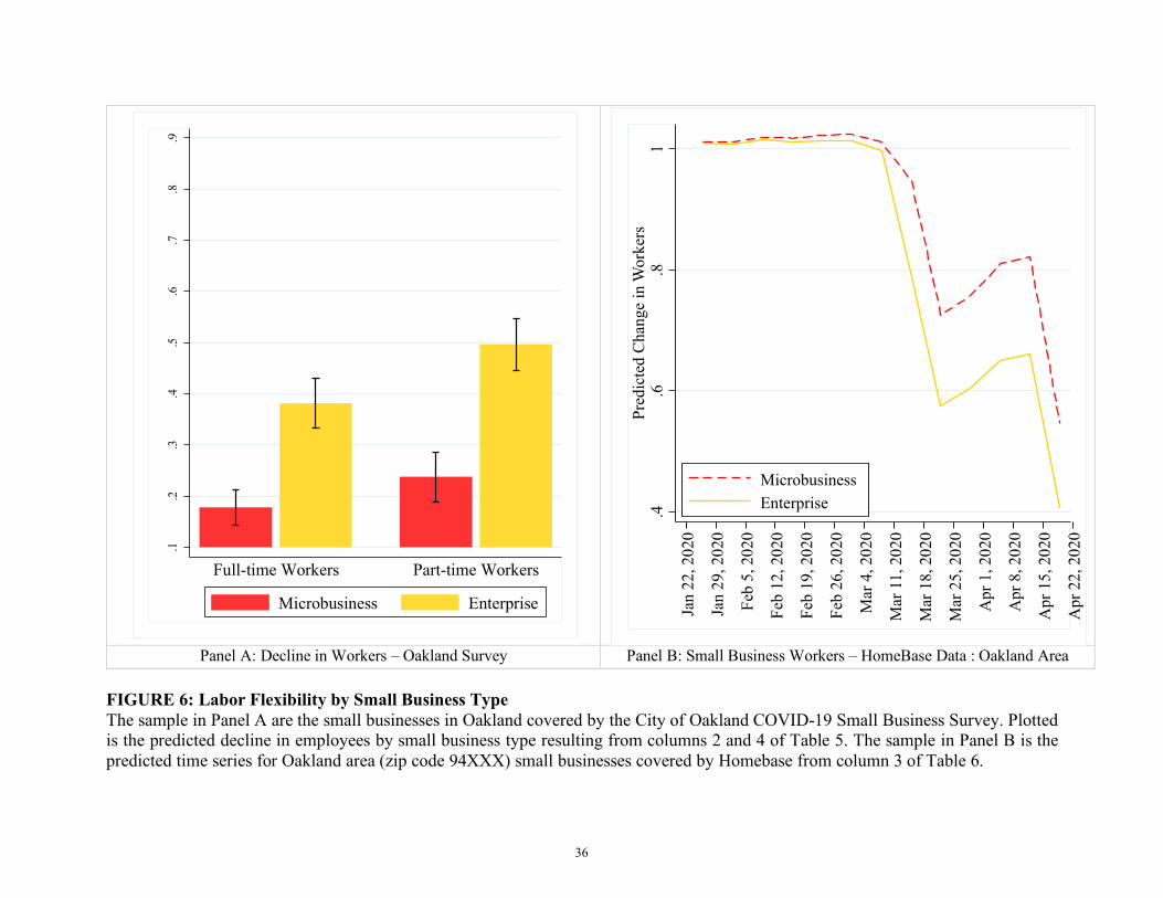
Panel A: Decline in Workers – Oakland Survey Panel B: Small Business Workers – HomeBase Data : Oakland Area

FIGURE 6: Labor Flexibility by Small Business Type The sample in Panel A are the small businesses in Oakland covered by the City of Oakland COVID-19 Small Business Survey. Plotted is the predicted decline in employees by small business type resulting from columns 2 and 4 of Table 5. The sample in Panel B is the predicted time series for Oakland area (zip code 94XXX) small businesses covered by Homebase from column 3 of Table 6.

.1.2

.3.4

.5.6

.7.8

.9

Perc

enta

ge D

eclin

e in

Wor

kers

Full-time Workers Part-time Workers

Microbusiness Enterprise

.4.6

.81

Pred

icte

d C

hang

e in

Wor

kers

Jan

22, 2

020

Jan

29, 2

020

Feb

5, 2

020

Feb

12, 2

020

Feb

19, 2

020

Feb

26, 2

020

Mar

4, 2

020

Mar

11,

202

0

Mar

18,

202

0

Mar

25,

202

0

Apr

1, 2

020

Apr

8, 2

020

Apr

15,

202

0

Apr

22,

202

0

date

MicrobusinessEnterprise

36

Panel C: Small Business Workers – Homebase National Panel D: Small Business Payroll – HomeBase National

FIGURE 6: (continued) Labor Flexibility by Small Business Type The sample are all U.S. business establishments covered by Homebase. Plotted is the predicted decline in workers (Panel C) and wages (Panel D) by small business type resulting from columns 6 and 9 of Table 6.

.4.6

.81

Pred

icte

d C

hang

e in

Wor

kers

Jan

22, 2

020

Jan

29, 2

020

Feb

5, 2

020

Feb

12, 2

020

Feb

19, 2

020

Feb

26, 2

020

Mar

4, 2

020

Mar

11,

202

0

Mar

18,

202

0

Mar

25,

202

0

Apr

1, 2

020

Apr

8, 2

020

Apr

15,

202

0

Apr

22,

202

0

date

MicrobusinessEnterprise .6

.7.8

.91

Pred

icte

d C

hang

e in

Wag

es

Jan

22, 2

020

Jan

29, 2

020

Feb

5, 2

020

Feb

12, 2

020

Feb

19, 2

020

Feb

26, 2

020

Mar

4, 2

020

Mar

11,

202

0

Mar

18,

202

0

Mar

25,

202

0

Apr

1, 2

020

Apr

8, 2

020

Apr

15,

202

0

Apr

22,

202

0

date

MicrobusinessEnterprise

37

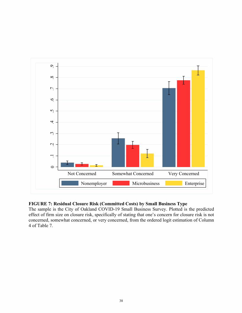
FIGURE 7: Residual Closure Risk (Committed Costs) by Small Business Type The sample is the City of Oakland COVID-19 Small Business Survey. Plotted is the predicted effect of firm size on closure risk, specifically of stating that one’s concern for closure risk is not concerned, somewhat concerned, or very concerned, from the ordered logit estimation of Column 4 of Table 7.

0.1

.2.3

.4.5

.6.7

.8.9

Mar

gina

l Eff

ect o

f Siz

e on

Clo

sure

Ris

k

Not Concerned Somewhat Concerned Very Concerned

Nonemployer Microbusiness Enterprise

38

FIGURE 8: Effect of Payroll Protection Program (PPP) on Medium-run Survival The sample is the City of Oakland COVID-19 Small Business Survey. Plotted is the predicted effect of firm size on medium-run survival, measured as the response to the question asking if circumstances do not change, how long can your firm survive from column 5 of Table 10, and taking into account the coefficients on Applied PPP, Success PPP, and Success PPP*LogEmployees.

-.20

.2.4

.6In

crea

se in

Pr(

Surv

ivin

g B

eyon

d Si

x M

onth

s)

0 2 4 6 8 10 12 14 16 18 20Pre-Crisis Employee Count

95% CI Marginal Effect

39

Table 1: City of Oakland COVID Survey of Small Business Summary Statistics

Panel A: EmploymentObs Mean StDev 0%ile 25%ile 50%ile 75%ile 100%ile

Nonemployer 1,014 0.250 0.433 0 0 0 0 1Microbusiness 1,014 0.430 0.495 0 0 0 1 1Enterprise 1,014 0.321 0.467 0 0 0 1 1Employees 1,014 6.52 9.81 0 1 2 8 50If microbusiness or enterprise…

Employees 761 8.68 10.46 1 2 4 11 50Full-time Employees 761 4.46 6.70 0 1 2 5 48Part-time Employees 761 4.22 6.75 0 0 2 5 40% Change Jobs Lost 761 0.177 0.256 0 0 0 0.421 1

Panel B: Gross ReceiptsObs Percentage Cumulative Percentage

Declining 1,014 0.523Percentage Change Gross Receipts in March Year-over-Year:

< 2% 6 0.007 0.0072 - 5% 7 0.008 0.0155 - 10% 30 0.035 0.05010 - 20% 53 0.061 0.11120 - 40% 168 0.194 0.306>40% 600 0.694 1.000

Observations with revenue decline data 864 1.000

Panel C: Business Closing RiskHow concerned are you about your business closing?Answers: Obs Percentage Cumulative Percentage

Not Concerned 40 0.039 0.039Somewhat Concerned 233 0.230 0.269Very Concerned 741 0.731 1.000

1,014 1.000

All data in Table 1 are from the City of Oakland COVID Survey of Small Business. Our sample is from March13, 2020 to April 1, 2020. As reported in Panel A, Nonemployer, Microbusiness and Enterprise classificationsare indicator variables dividing the sample into those with no employees, those with 1-5 employees, and thosewith 6-50 employees, respectively. Employees are reported as exisitng in early March (pre-crisis). The smallersample in Panel A, 761 firms, are those with positive employment. For this sample, we know the existing base ofpart-time and full-time employees and the jobs lost. Panel B presents two pictures of gross receipts. First iswhether the business is declining in gross receipts, defined as reporting the year-over-year receipts as of Februaryas being in decline relative to 2019. A smaller sample responded to the question as to the declines in March at the initial sheltering in place. The survey asked owners to report their gross receipts in March year-over-year fromMarch 2019. Panel C presents closure risk responses. In particular, the survey respondents were asked howconcerned they were about closing the business, responding in the categories listed below.

40

Table 2: Oakland Manual Data Collection Summary Statistics

Panel A: IndustryObs Percentage

Business services 82 8.1%Construction / fabrication / venues / workspaces 95 9.4%

Fitness / gym / wellness 86 8.5%Medical offices 38 3.7%Personal services home 28 2.8%Personal services shop 75 7.4%Professional services 206 20.3%Restaurant 156 15.4%Retail 144 14.2%Salon 104 10.3%

1,014 100.0%

Panel B: Commerce Location and Essential DesignationObs Percent

Main Street 674 0.665At a Venue, Home, or Offsite 340 0.335

1,014 1.000

Essential Business under Shelter-in-Place 1,262 0.110

Panel C: Interim Outcome Obs Percent Cumulative PercentPermanently Closed or Lacking Ongoing Concern Signal 159 0.192 0.192Temporarily Closed 211 0.255 0.447Trying 172 0.208 0.655Open 285 0.345 1.000

827 1.000

Auto repair, car wash, child care, education, laundry, tattooArchitects, consultants, desginers, engineers, lawyersRestaurantsRetail shopsSalons, barbers

Chiropractic, dentist, optical, physical therapy, psychologyHome repair, landscape, pet walking, realty

Presented are the manual lookup data for businesses in the City of Oakland COVID Survey. We manually codedall fields -- industry, location, whether the business is essential under Alameda County's shelter-in-place order,and outcome status by a two step process. We always invoke both steps. First we looked up the establishment inGoogle Maps. Second, we went the to business website (always) and other Internet sites where information mightbe available (if necessary), including yelp and blogs of closures.

ExamplesCatering, industrial cleaning, printing, photography, technologyConstruction, entertainment venues, event spaces, parking lots, housing, manufacturing, wholesale tradeFitness centers, gyms, massage, acupuncture

41

Table 3: Homebase Employee Data and SafeGraph Foot Traffic Data Summary Statistics

Panel A: Homebase Employee Headcounts(1) (2) (3) (4) (5) (6) (7) (8)

Homebase Industry Obs Mean StDev 50%ile Obs Mean StDev 50%ile

Beauty & Personal Care 417 4.34 4.29 3.0 235 $1,093 $1,344 $692Charities, Education & Membership 1,430 8.55 8.16 6.0 1,013 $2,084 $3,298 $1,168Food & Drink 23,159 9.21 7.41 7.3 16,761 $2,491 $2,742 $1,731Health Care and Fitness 3,934 5.57 5.44 4.0 2,520 $2,086 $2,782 $1,189Home and Repair 579 5.10 5.82 3.2 409 $2,574 $3,290 $1,753Leisure and Entertainment 936 7.91 7.95 5.3 735 $2,038 $2,523 $1,175Other 4,189 7.09 7.48 4.5 2,972 $2,725 $4,522 $1,468Professional Services 1,986 5.07 5.88 3.2 1,333 $2,470 $4,817 $1,183Retail 8,649 5.46 5.13 4.0 5,962 $2,397 $3,464 $1,354Transportation 373 6.79 7.43 4.2 261 $3,577 $4,741 $1,859Unknown 4,797 7.19 6.46 5.2 3,262 $2,157 $2,797 $1,282All 50,449 7.60 6.98 5.5 35,463 $2,413 $3,197 $1,510

Panel B: SafeGraph Foot Traffic

Industry Obs Mean StDev 0%ile 25%ile 50%ile 75%ile 100%ile

Business services 5 3.89 2.32 1.31 2.55 3.42 4.82 7.35Construction / fabrication / venues / workspaces 19 6.54 5.54 0.41 1.31 5.01 11.64 16.15Fitness / gym / wellness 28 4.83 4.65 0.35 1.23 3.37 7.48 18.25Medical offices 4 0.85 0.43 0.46 0.56 0.74 1.14 1.46Personal services 14 5.73 5.50 0.69 1.96 4.85 6.63 21.47Professional services 7 5.12 7.51 0.56 0.68 2.54 4.20 21.85Restaurant 114 7.55 8.31 0.10 3.31 5.37 8.46 59.68Retail 67 4.90 4.45 0.28 1.23 4.00 6.53 17.38Salon 10 2.52 3.00 0.40 0.89 1.46 3.19 10.50Total 268 6.02 6.63 0.10 1.83 4.17 7.48 59.68

Panel A presents summary statistics for the sample of small businesses provided by HomeBase, tabulatedseparately by HomeBase industry. Columns 1 - 4 present mean and median employee headcount during theperiod January 1, 2020 and February 15, 2020. Columns 5-8 present statistics for total weekly wages during thissame time period for those firms within HomeBase that reported wages for some or all employees. Panel Bpresents summary statistics by coded industry for daily foot traffic for 268 small businesses in the Oaklandsurvey that could be matched to a Point of Interest (POI) within the SafeGraph dataset. Daily foot traffic isdefined as reported visits per day to a POI between January 1, 2020 and March 15, 2020, scaled by the number ofdevices observed by SafeGraph in Alameda County per 100,000 residents.

Employees Weekly Wages

42

Table 4: Revenue Resiliency

(1) (2) (3) (4) (5) (6)Dependent Variable:

Log Workers 0.0126** 0.0274*** 0.0099 0.0271***[0.00616] [0.00895] [0.0071] [0.0103]

Nonemployer 0.0538** 0.0593**[0.0246] [0.0261]

Post -1.344*** -1.193***[0.109] [0.139]

Post*Log Workers -0.0673 -0.126**[0.0435] [0.0543]

Post*Nonemployer -0.334*[0.192]

Log Receipts Decline February 0.217*** 0.225*** 0.219*** 0.231***[0.0402] [0.0403] [0.0408] [0.0412]

Main Street 0.0299* 0.0274 0.0544 0.0651[0.0166] [0.0167] [0.0799] [0.0732]

Essential -0.0107 -0.00738 0.00233 0.00327[0.0207] [0.0201] [0.0265] [0.0266]

Business services -0.0673 -0.0842[0.0889] [0.0835]

Construction / Manuf / Venue 0.0059 -0.00359[0.0326] [0.0336]

Fitness/gym/wellness -0.0148 -0.0302[0.0868] [0.0812]

Medical Offices -0.00796 -0.0187[0.0986] [0.0923]

Personal services home -0.0495 -0.0728[0.0473] [0.0499]

Personal services shop -0.0641 -0.0805[0.0924] [0.0865]

Restaurant -0.0118 -0.0367[0.0851] [0.0798]

Retail -0.0348 -0.0477[0.0823] [0.0763]

Salon -0.0162 -0.0387[0.0847] [0.0794]

Firm Fixed Effects Yes YesDay Fixed Effects Yes YesObservations 349 349 349 349 23,292 23,292R-squared 0.107 0.120 0.125 0.139 0.796 0.797

Presented are two sets of revenue resiliency results for the City of Oakland. Columns 1-4 report estimations from the Cityof Oakland COVID Small Business Survey. The dependent variable is the reported revenue percentage change decline ingross decline, calculated as the natural logarithm of 1 + percentage change reported YoY for March 2020. We control forthe same variable for February to focus on the March crisis impact. The main independent variables are the log of workers(employees +1) and a nonemployer indicator, per the Oakland survey data. In columns 1-2, we include an indicator for thebusiness being main street-facing and one for essential business, both from manual coding. Columns 3-4 add in detailedindustry fixed effects, reported below for interest. Robust standard errors in columns 1-4 are in brackets. Columns 5-6report difference-in-differences estimates of the foot traffic decline for the same businesses in Oakland, including firm andday fixed effects. Standard errors in columns (5)-(6) are clustered by firm in brackets. *,**,and *** indicate significancelevels of 10%, 5%, and 1%.

Log (1+ % Decline YoY Receipts, March 2020) Log (Foot Traffic)

43

Table 5: Labor Flexibility - Oakland Survey

(1) (2) (3) (4) (5) (6)Model:

Dependent Variable:

Log Workers 0.117*** 0.127*** 0.128*** 0.165*** 0.172*** 0.173***[0.0150] [0.0168] [0.0167] [0.0207] [0.0238] [0.0237]

Revenue Loss Index 0.0769*** 0.0692*** 0.0844* 0.0680*** 0.0696*** 0.117*[0.0200] [0.0193] [0.0452] [0.0239] [0.0243] [0.0685]

Log Workers * Rev Loss Index -0.00749 -0.0214[0.0196] [0.0306]

Main Street 0.0718** -0.0238 -0.0275 0.0435 -0.0893 -0.104[0.0360] [0.174] [0.175] [0.0484] [0.244] [0.243]

Essential -0.0842* -0.0636 -0.0651 -0.137** -0.184** -0.189***[0.0443] [0.0604] [0.0613] [0.0581] [0.0714] [0.0727]

Business services 0.0105 0.0141 0.159 0.176[0.174] [0.174] [0.254] [0.252]

Construction / Manuf / Venue -0.017 -0.0165 -0.00468 -0.00233[0.0611] [0.0609] [0.0841] [0.0828]

Fitness/gym/wellness 0.0791 0.0819 0.0436 0.0554[0.182] [0.181] [0.240] [0.237]

Medical Offices 0.0236 0.0288 0.165 0.183[0.211] [0.213] [0.299] [0.297]

Personal services home -0.0374 -0.0375 -0.0837 -0.0844[0.112] [0.112] [0.129] [0.127]

Personal services shop 0.0859 0.0904 0.176 0.194[0.186] [0.187] [0.254] [0.252]

Restaurant 0.053 0.0567 0.0898 0.105[0.172] [0.172] [0.240] [0.236]

Retail 0.0783 0.0827 0.191 0.209[0.168] [0.169] [0.233] [0.230]

Salon 0.286 0.288 0.102 0.118[0.194] [0.192] [0.246] [0.243]

Observations 556 556 556 442 442 442R-squared 0.099 0.117 0.118 0.096 0.103 0.104

Fractional Logit: Reporting Marginal Effect

The sample is small business respondents for the City of Oakland COVID Small Business Survey. The dependentvariable in columns 1-3 (4-6) is the reported percentage change in full-time (part-time) workers. The mainindependent variables is the log of workers (employees +1). Nonemployer data are not included because of the lackof employees. Included in all columns are an indicator for the business being main street-facing and one for essentialbusiness, both from manual coding. Also included is the revenue loss index variable, the combination of standardized firm revenue losses from the gross receipts decline and standardized percentage change in foot traffic by firm.Columns 3 and 6 include this variable interacted with workers. Columns 2,3,5, and 6 add in detailed industry fixedeffects. Robust standard errors are in brackets. *,**,and *** indicate significance levels of 10%, 5%, and 1%.

Percentage Change Decline in Part-Time Workers

Percentage Change Decline in Full-Time Workers

44

Table 6: Labor Flexibility - Homebase Payroll Data

(1) (2) (3) (4) (5) (6) (7) (8) (9)

Dependent Variable:

Post -0.443*** -0.416*** -0.429*** -0.505*** -0.497*** -0.510*** -1.871*** -1.880*** -1.924***[0.0609] [0.0708] [0.126] [0.00881] [0.0101] [0.0174] [0.0231] [0.0260] [0.0456]

Post * LogWorkersPre -0.289*** -0.288*** -0.279*** -0.303*** -0.302*** -0.294*** -0.251*** -0.252*** -0.228***[0.0269] [0.0271] [0.0725] [0.00373] [0.00375] [0.0102] [0.00869] [0.00874] [0.0220]

Log Foot Traffic 0.0486*** 0.0538*** -0.0149 0.0437*** 0.0449*** -0.0319*** 0.0594*** 0.0581*** -0.0175[0.0126] [0.0132] [0.0292] [0.00180] [0.00186] [0.00470] [0.00417] [0.00431] [0.0116]

Post * Log Foot Traffic -0.00981 -0.0421 -0.00246 -0.0259*** 0.00289 -0.00848[0.0166] [0.0395] [0.00184] [0.00481] [0.00442] [0.0129]

LogWorkersPre * Log Foot Traffic 0.0358** 0.0413*** 0.0380***[0.0171] [0.00288] [0.00577]

Post*LogWorkers*LogFootTraffic 0.016 0.0122*** 0.00546[0.0230] [0.00292] [0.00639]

Firm Fixed Effects Yes Yes Yes Yes Yes Yes Yes Yes YesDay Fixed Effects Yes Yes Yes Yes Yes Yes Yes Yes YesObservations 16,760 16,760 16,760 714,039 714,039 714,039 460,630 460,630 460,630# of Businesses 1,428 1,428 1,428 60,544 60,544 60,544 39,210 39,210 39,210R-squared 0.836 0.836 0.837 0.835 0.835 0.836 0.899 0.899 0.899

The sample is the set of firms in the national Homebase data, matched to the industry-zip code data in SafeGraph. In columns 1-3, the sample is further restricted to thefirms in the Oakland area (zip codes 94XXX). Observations are a weekly panel from January 2020 through April 2020. The dependent variable in columns 1-6 is thelog of workers, and in columns 7-9, the log of payroll The main independent variable is the log of workers pre-crisis interacted with post. Firm and week fixed effectsare included. Post indicates weeks after March 15, 2020. Log foot traffic is from SafeGraph and is matched to Homebase at the industry-zip code level. Nonemployerdata are not included because of the lack of employees. Firm-clustered standard errors are in brackets. *,**, and *** indicate significance levels of 10%, 5%, and 1%.

Log Workers, Oakland Area Sample Log Payroll, National SampleLog Workers, National Sample

45

Table 7: Committed Costs Results -- Residual of Closure Risk

(1) (2) (3) (4)Model:

Dependent Variable:

Log Workers 0.251*** 0.195 0.212** 0.165*[0.0910] [0.128] [0.105] [0.0975]

odds ratio: 1.285 1.215 1.236 1.179

Nonemployer -0.192[0.305]

Revenue Loss Index 0.323*** 0.326*** 0.322*** 0.318***[0.0947] [0.0952] [0.117] [0.0949]

Jobs Lost % Change 0.774* 0.765 0.735** 0.668[0.462] [0.469] [0.307] [0.467]

Interim Outcomes:Trying 0.519** 0.530** 0.364 0.125

[0.261] [0.263] [0.400] [0.288]Temporarily Closed 0.987*** 0.986*** 0.878* 0.679**

[0.275] [0.275] [0.469] [0.312]Permanently Closed 0.561** 0.557** 0.442* 0.248

[0.245] [0.245] [0.251] [0.263]Declining 0.879*** 0.884*** 0.851*** 0.807***

[0.187] [0.187] [0.195] [0.190]Main Street 0.447** 0.447** 0.452** 0.0565

[0.218] [0.218] [0.214] [1.240]

Industry Effects random fixed

Observations 736 736 736 736R-squared 0.086 0.087 n/a 0.107

The sample is small business respondents for the City of Oakland COVID Small Business Survey. The dependent variableis the ordinal response of how concerned the business owner is about closure risk: not concerned, somewhat concerned,and very concerned. The is an ordered logit, presenting the log odds ratios (the coefficients) of moving from one categoryup to the next. We also report the odds ratio, beneath the robust standard errors in brackets for the main independentvariable of log workers (employees +1). Included in all columns are an indicator for the business being main street-facingand the percentage change jobs reported. Also included is the revenue loss index variable and whether the business wasdeclining pre-crisis (using the gross receipts YoY for February), and the interim outcome of the business {Open, Trying,Temporarily Closed, Permanently Closed}. Columns 3 and 4 are industry random and fixed effects, respectively. (Fixedeffects for ordered logit are of questionable consistency; thus we present the random effects as a more reliable estimator.)*,**,and *** indicate significance levels of 10%, 5%, and 1%.

Ordered LogitClosure Risk: Not Concerned < Somewhat Concerned < Very Concerned

46

Table 8: City of Oakland Re-opening and Recovery Survey Summary StatisticsPresented are the tabulations of the 278 survey responses from the City of Oakland Re-opening and Recovery Survey.

Count Percentage CumulativeTotal Oakland Survey Responses 278

0 to 1 month 26 9.4 9.41 to 3 months 85 30.6 39.93 to 6 months 71 25.5 65.56 to 12 months 55 19.8 85.3Never 41 14.8 100.0

Short-Term ClosingOngoing Concern 250 89.9Closed Now or Projected Survival of 0-to-1 month 28 10.1

Medium-Run SurvivalSurviving 96Closing 182

Application Status of Payroll Protection Program (PPP)Successfully Applied 148 59.4 59.4Unsuccessfully Applied 45 18.1 77.5Not Applied 56 22.5 100.0

77%Application Status of Pandemic Unemployment Insurance (PUI)

Successfully Applied 82 32.9 32.9Unsuccessfully Applied 39 15.7 48.6Not Applied 128 51.4 100.0

68%

Status as of June 2020Fully Open 20 7.2Reduced 120 43.2Closed, at least Temporarily 138 49.6

IndustryBusiness Services 7 2.5Construction/Industrial/Venue 18 6.5Fitness/Salon/Wellness 59 21.2Healthcare 17 6.1Nonprofit 15 5.4Personal Services 14 5.0Professional Services 55 19.8Restaurant 61 21.9Retail 32 11.5

Gender IdentityFemale 171 61.5Male 74 26.6Other / Undisclosed 33 11.9

Race / EthnicityAsian Ethnicity 48 17.3Hispanic Ethnicity 21 7.6White Race 120 43.2Black Race 31 11.2Other / Undisclosed / Mixed Race 58 20.9

“If business disruption continues at the current rate, how soon will you be at risk of permanently closing your business?"

Acceptance Rate

Acceptance Rate

47

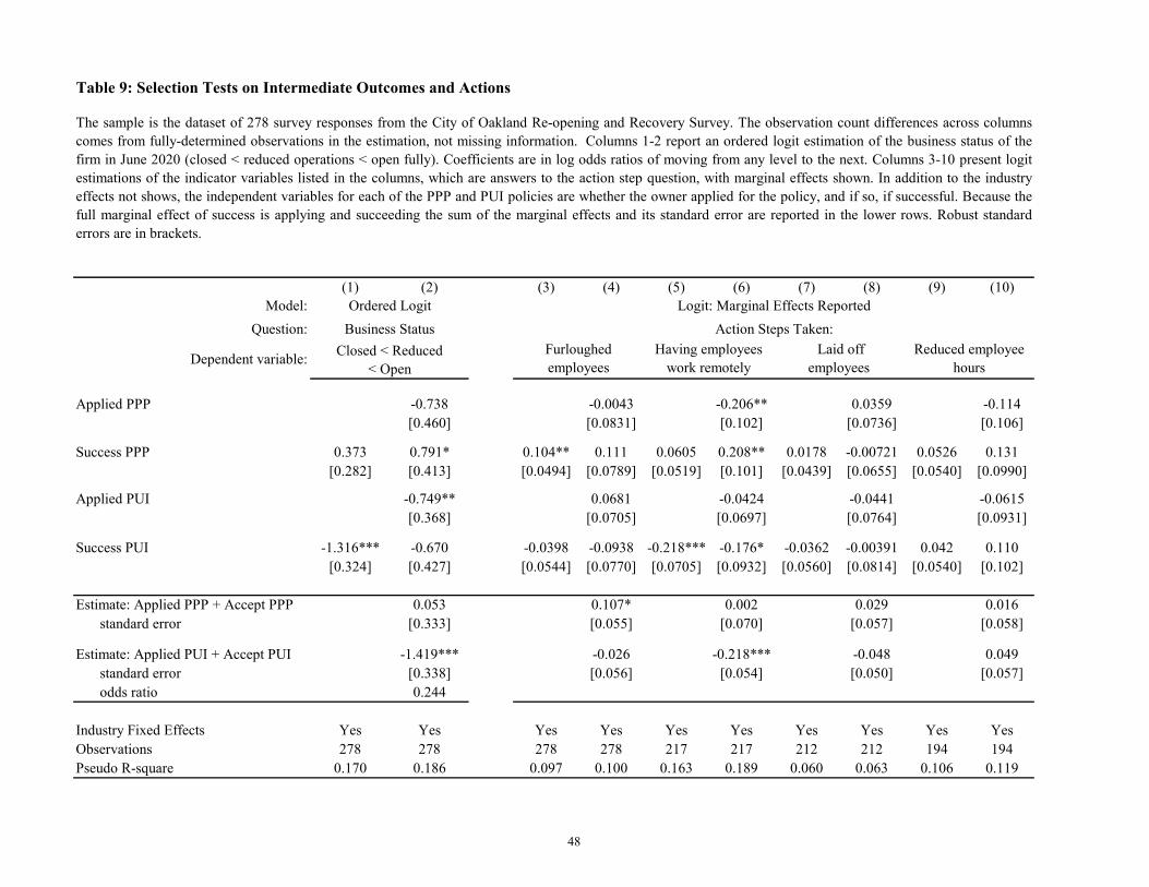
Table 9: Selection Tests on Intermediate Outcomes and Actions

(1) (2) (3) (4) (5) (6) (7) (8) (9) (10)Model:

Question:

Dependent variable:

Applied PPP -0.738 -0.0043 -0.206** 0.0359 -0.114[0.460] [0.0831] [0.102] [0.0736] [0.106]

Success PPP 0.373 0.791* 0.104** 0.111 0.0605 0.208** 0.0178 -0.00721 0.0526 0.131[0.282] [0.413] [0.0494] [0.0789] [0.0519] [0.101] [0.0439] [0.0655] [0.0540] [0.0990]

Applied PUI -0.749** 0.0681 -0.0424 -0.0441 -0.0615[0.368] [0.0705] [0.0697] [0.0764] [0.0931]

Success PUI -1.316*** -0.670 -0.0398 -0.0938 -0.218*** -0.176* -0.0362 -0.00391 0.042 0.110[0.324] [0.427] [0.0544] [0.0770] [0.0705] [0.0932] [0.0560] [0.0814] [0.0540] [0.102]

Estimate: Applied PPP + Accept PPP 0.053 0.107* 0.002 0.029 0.016standard error [0.333] [0.055] [0.070] [0.057] [0.058]

Estimate: Applied PUI + Accept PUI -1.419*** -0.026 -0.218*** -0.048 0.049standard error [0.338] [0.056] [0.054] [0.050] [0.057]odds ratio 0.244

Industry Fixed Effects Yes Yes Yes Yes Yes Yes Yes Yes Yes YesObservations 278 278 278 278 217 217 212 212 194 194Pseudo R-square 0.170 0.186 0.097 0.100 0.163 0.189 0.060 0.063 0.106 0.119

Business Status Action Steps Taken:

The sample is the dataset of 278 survey responses from the City of Oakland Re-opening and Recovery Survey. The observation count differences across columnscomes from fully-determined observations in the estimation, not missing information. Columns 1-2 report an ordered logit estimation of the business status of thefirm in June 2020 (closed < reduced operations < open fully). Coefficients are in log odds ratios of moving from any level to the next. Columns 3-10 present logitestimations of the indicator variables listed in the columns, which are answers to the action step question, with marginal effects shown. In addition to the industryeffects not shows, the independent variables for each of the PPP and PUI policies are whether the owner applied for the policy, and if so, if successful. Because thefull marginal effect of success is applying and succeeding the sum of the marginal effects and its standard error are reported in the lower rows. Robust standarderrors are in brackets.

Logit: Marginal Effects ReportedOrdered Logit

Closed < Reduced < Open

Furloughed employees

Having employees work remotely

Laid off employees

Reduced employee hours

48

Table 10: Are PPP and Pandemic Unemployment Insurance Programs Saving Businesses?

(1) (2) (3) (4) (5) (6) (7)Dependent Variable:

Model: Linear Probability

Applied PPP 0.0163 0.0161 -0.268*** -0.294*** -0.192*[0.0582] [0.0629] [0.104] [0.110] [0.0989]

Accept PPP 0.0573 0.0606 0.053 0.268** 0.473*** 0.533*** 0.387***[0.0717] [0.0825] [0.0797] [0.105] [0.142] [0.150] [0.144]

Accept PPP * LogWorkers -0.0206 -0.0232 -0.0166 -0.133** -0.139** -0.185*** -0.129**[0.0431] [0.0435] [0.0206] [0.0540] [0.0561] [0.0586] [0.0569]

Applied PUI 0.0641 0.0495 -0.0344 -0.131 0.0119[0.0571] [0.0619] [0.0779] [0.0833] [0.0789]

Accept PUI -0.168** -0.205** -0.142* -0.176* -0.155 -0.104 -0.154[0.0756] [0.0827] [0.0819] [0.105] [0.123] [0.136] [0.123]

Accept PUI * Log Workers 0.164*** 0.159*** 0.129** -0.107 -0.0861 -0.0139 -0.0788[0.0445] [0.0436] [0.0505] [0.0817] [0.0793] [0.0813] [0.0682]

LogWorkers -0.0162 -0.0135 0.00343 0.144*** 0.158*** 0.169*** 0.136***[0.0444] [0.0452] [0.0139] [0.0488] [0.0506] [0.0523] [0.0508]

Nonemployers -0.0473 -0.0501 -0.0369 0.185* 0.224** 0.247** 0.183*[0.0731] [0.0711] [0.0626] [0.106] [0.101] [0.101] [0.105]

Fixed Effects Included:Industry Yes Yes Yes Yes Yes Yes YesGender Identity Yes Yes Yes Yes Yes Yes YesRace/ Ethnicity Yes Yes Yes Yes Yes Yes YesStatus -- -- -- -- -- -- YesAction Steps -- -- -- -- -- -- -- YesDrops Furloughing Firms -- -- -- -- -- Yes --

Observations 238 238 278 278 278 222 278Pseudo R-square 0.277 0.288 0.208 0.210 0.237 0.279 0.268

The sample is the City of Oakland Re-opening and Recovery Survey. All estimations are logits, presenting marginal effects.Both dependent variables build off the survey question: “If business disruption continues at the current rate, how soon will yoube at risk of permanently closing your business?” The column 1-2 dependent variable, short-term closing, is an indicator equalto 1 if the answer to this question is 0-to-1 month or if the respondent indicates elsewhere that s/he is permanently closedalready. The dependent variable in columns 3-4, medium-run surviving, is equal to one if the answer to the question is greaterthan 6 months. The main independent variables are LogWorkers, equal to the natural log of employees plus 1 (the owner),whether the owner took a PPP, and whether the owner took Pandemic Unemployment Insurance, and the interactions of theseprogram variables with LogWorkers. We control for race, gender identity, industry, and reported company status (closed,trying but reduced, or open). Robust standard errors are in brackets. *** p<0.01, ** p<0.05, * p<0.1

Medium-run SurvivingLogit Marginal

Effects Logit Marginal Effects

Short-term Closing

49