Embed Size (px)
Citation preview
1
Corso di Laurea magistrale in Amministrazione, finanza e controllo
Tesi di Laurea
Managed Volatility Funds By Morningstar Investment Management
Relatore Chiar. ma Prof. ssa Elisa Cavezzali
Correlatore Chiar. mo Prof. Ugo Rigoni Laureanda Cristina Borghilli Matricola 823589
Anno Accademico 2013 / 2014
2
Table of contents
Introduction………………………………………………………..……………………...…p.6
Chapter 1 –MUTUAL FUNDS................................................................................p.10
1.1 Introduction........................................................................................................p.10
1.2 Asset management ……………………………………………………………………p.11
1.2.1 Asset management definition......................................................................p.11
1.2.2 The asset management market in Italy…………………………...………..…p.13
1.2.3 A global comparison……………………………………………………....……p.17
1.3 Mutual funds………………………………………………………………...………...p.18
1.3.1 Mutual funds definition ……………………………………..….………….…..p.18
1.3.2 Main actors in the market of mutual funds…………………………...……...p.19
1.3.3 The scenario of development of mutual funds…………………………….…p.21
1.3.4 Mutual funds in Italy……………………………………………………..……..p.24
1.3.5 Advantages of mutual funds……………………………………………………p.25
1.4 Categories and costs of mutual funds and life insurance plans….………….….p.27
1.4.1 Mutual funds classification in Italy……..…………………….……..............p.27
1.4.2 Other categories of mutual funds………………...……………….…………..p.32
1.4.3 Mutual funds costs……………………………..………..………………...……p.35
1.4.4 The binomial insurance-mutual fund………….………….…………..………p.36
1.4.5 Unit linked insurance plan…………………………….…..………………..…p.37
1.5 Financial markets………………..……………………………..………………….....p.38
1.5.1 Regulated and OTC market…………………………………………………....p.38
1.5.2 Market indices…………………..…………………………….…………………p.39
Chapter 2 –CML, CAPM AND PERFORMANCE MEASUREMENTS………....p.43
2.1 Introduction…………………………………………………….………….………..…p.43
2.2 The modern portfolio theory (MPT)…..…...………… ……………...…………....p.44
2.2.1 Introduction to the MPT……….…….……………………………...………....p.44
3
2.2.2 Mean-variance and expected utility………………………………………..…p.46
2.3 Measuring risk and return………………………………………………………..…p.49
2.3.1 Risk and return of a two-asset portfolio………………………………...……p.49
2.3.2 Asset allocation with two risky assets…………………………………...……p.50
2.3.3 Introducing a risky-free asset and the Tobin’s separation theorem: the
CML…………………………………………………………………………………...…p.53
2.3.4 From the CML to the SML: the Capital Asset Pricing Model...………..…p.57
2.3.6 Asset allocation with N risky assets………………………………………..…p.59
2.3.6.1 Asset allocation with N risky assets and a riskless asset……………..p.59
2.3.6.2 Efficient frontier with N risky assets and no riskless asset……….….p.62
2.3.7 Systematic and unsystematic risk………………………………..…...…….....p.64
2.4 Mean variance optimization pitfalls…………………………...………………...…p.67
2.4.1 Behavioral economics’ critique………………………..…………………...…p.67
2.4.2 The Single Index Model………………………..…………………………...…..p.69
2.4.3 The Black-Litterman model……………………………………….............…..p.73
2.4.4 Roll’s critique………………………………………………….……..………....p.73
2.5 The benchmark and the portfolio management strategy………..………………..p.74
2.6 Performance and risk measurement……………………….…………...………..…p.78
2.6.1 Introducing performance and risk measurement………………...………....p.78
2.6.2 The Sharpe Index………………………………………….……….………...….p.79
2.6.3 The Treynor ratio…………………………………………….…….………..….p.80
2.6.4 Value at risk (VaR)………………………………….……….…….………...….p.81
2.6.5 Modigliani RAP index ……………………………………………………....…p.81
2.6.6 Jensen’s alpha …………………………………………………….………….....p.82
2.6.7 Portfolio’s beta………………………….………………………….………..….p.83
2.6.8 Information ratio………………………..………………………….………..….p.83
Chapter 3 –CLERICAL MEDICAL’S MANAGED PORTFOLIOS BY
MORNINGSTAR……….........................................................................................p.85
3.1 Introduction ………………………………………………………………...…………p.85
3.2 Morningstar, Inc.…………………………………………….…………………..…...p.86
3.2.1 The company ……..……………………………………………….…………….p.86
3.2.2 Morningstar Style Box…………………………..……………………….…….p.87
4
3.2.3 Morningstar star rating………………………………………….…..……..….p.89
3.2.4 Morningstar analyst rating for funds…………………….…….…………….p.91
3.3 Clerical Medical managed funds by Morningstar Investment
Management…………………………………………..…………………….……………..p.94
3.3.1Clerical Medical, the company …………..…………….…..….…………..….p.94
3.3.2 The funds……………………………………………………..….…………….…p.96
3.3.3 Morningstar strategic asset allocation…………………….….………..…….p.97
3.3.3.1 Markowitz 2.0 ……………………………………………..………..……..p.97
3.3.3.2 Asset allocation for Clerical Medical funds…………………….……p.103
3.3.4 Morningstar fund selection and portfolio construction……….……...…..p.105
3.3.4.1 Selection of funds and portfolio construction for the solution for
Clerical Medical………………………………………………..…..…………….p.108
3.3.5 Dynamic asset allocation……………………………………………....……..p.335
3.3.6 Daily monitor and rebalancing………………………………………….…..p.117
3.4 Performance………………………………………………………………………….p.118
Chapter 4 –PORTFOLIO MANAGEMENT ANALYSIS….................... p.123
4.1 The CMIG Adventurous Managed Fund and the BG Selection Global Risk
Managed Fund……………………………………………………………………………p.123
4.1.1 The proxy of the CMIG Adventurous portfolio……………….……….…...p.123
4.1.2 The benchmark …………………………………………………….…….…….p.126
4.1.3 Performance ……………………………..…………………………..……..….p.128
4.2 The analysis………………………………………………………………….……….p.129
4.2.1 The aim of the analysis ……………………………………………….………p.129
4.2.1.1 Asset allocation and fund selection of the comparison
portfolio……………………………………………………………….……….…..p.130
4.2.1.2 Portfolio construction………………………………………….…….….p.133
4.2.1.3 The efficient frontier……………………………………………….…….p.136
4.2.1.4 The optimal portfolio………………………………………………..…..p.140
4.3 A comparison of the two portfolios……………………………………….…...….p.142
4.3.1 Asset allocation…………………………………………………………….…..p.142
4.3.2 Performance …………………………………………………………..….……p.144

5
4.4 Performance indices and risk indices…………………………………………..…p.148
4.4.1 The importance of the indices………………………………………………..p.148
4.4.2 The Sharpe index……………………………………………………………....p.148
4.4.3 The Treynor ratio ……………………………………………………….…….p.149
4.4.4 Modigliani RAP index…………………………………………………………p.150
4.4.5 Jensen’s alpha …………………………………………………………………p.151
4.4.6 Volatility…………………………………………………………….…………..p.151
4.4.7 Portfolio’s beta…………………………………………………..…………….p.152
4.4.8 Information ratio…………………………………………………………..…..p.153
Conclusions……………………………………..…………………………………………p.154
Bibliography...........................................................................................................p.159
Bibliography of websites.....................................................................................p.164
6
Introduction
The global assets of the mutual fund industry have grown more than sevenfold in
the last two decades: from 4 trillion dollars in 1993 to 28.9 trillion dollars in September
2013, with an increase in each of the four broad regions, e.g. the United States, Europe,
Asia Pacific and the rest of the world. The boom of mutual funds is favored by factors
like the improving levels of economic development, deep liquid markets and the
existence of a defined contribution plan system that enables participants to invest in
mutual funds. Moreover, demographic factors like the aging of the population in
developed and developing countries make retirement schemes increasingly
unsustainable, driving investors to grow a demand for mutual funds as a savings vehicle
(Plantier, 2013). In Italy, the mutual fund industry expanded between 1995 and 2000
with the reduction of interest rates of Italian Treasury Bonds (BOT, Buoni Ordinari del
Tesoro), which led investors to look for investment instruments different from the
traditional ones.
Mutual funds are extremely flexible instruments that are totally adaptable to the
specific request of each investor. In fact they grant the advantage of allowing even to
small household investors to get close to stock markets, investing in a diversified
portfolio managed by a professional manager. Mutual funds classification in Italy is
currently held by Assogestioni, the representative association of the Italian investment
management industry, that classifies mutual funds according to the percentage of stocks
held in the portfolio. The five broad categories of mutual funds are stock or equity
funds, balanced funds, bond funds, money market funds and flexible funds. Equity
funds invest at least 70% in stocks, balanced funds invest from 10% to 90% in stocks,
bond funds and money market funds do not invest in stocks, and flexible funds do not
have any constraint on the percentage of stocks to keep in the portfolio.
The mutual fund industry has become a highly competitive industry, and the
range of products that are offered is constantly growing. It is necessary both for
7
individual investors and institutional investors that act on behalf of their clients to
choose the best portfolio of assets. The concept of asset allocation has been a hot topic
in the last decades, and the mean-variance (MV) analysis of Harry Markowitz (1952)
with his Modern Portfolio Theory (MPT) is considered to set the birth of modern
finance. The theory was further developed by Sharpe in the Capital Asset Pricing Model
(CAPM). The idea behind the two cited models is the relationship between risk and
return (higher expected returns are obtained increasing the level of risk of the portfolio)
and the trade-off relationship between the maximization of portfolio returns and the
minimization of portfolio risk. Besides, they are based on the notion that investors act
rationally considering all available information, that markets are efficient and that
security prices reflect all available information. These theories are still state of the art
for most practitioners and many academic circles but are encountering critics by schools
of thought like behavioral economics.
Our analysis studies the innovative target volatility approach that the investment
management company Morningstar Investment Management applies to three portfolios
of funds (funds of funds) to face the actual instability of financial markets. Morningstar
Investment Management is a division of Morningstar, Inc., an investment research firm
headquartered in Chicago that provides data on investment offerings and whose main
activity is to supply information over mutual funds to Microsoft Money Central,
American Online and Yahoo Finance. In addition to this, it also provides classifications
of mutual funds and fund-ratings. Examples are the Morningstar Style Box, the
Morningstar star rating and the Morningstar analyst rating for funds. The investment
division of Morningstar, Morningstar Investment Management, has the advantage of
having at its disposition a very large amount of information owned by the company
itself, that is already selected and interpreted by researchers internal to the company.
The portfolios under analysis are managed since March 2013 by Morningstar
Investment Management for the insurance company Clerical Medical. Clerical Medical
is a British company specialized in insurance and financial products and it is part of the
Lloyds Banking Group. The managed portfolios are three funds of funds with an
increasing risk profile (defined by the increasing percentage of equity funds held in the
portfolio): CMIG Euro Cautious Managed, CMIG Euro Balanced Managed, CMIG
Euro Adventurous Managed. The portfolios are created with the innovative optimization
model Markowitz 2.0, that is explained by Kaplan (2011), one of the main experts
8
behind the elaboration of the Morningstar rating and the Morningstar Style Box. The
model is valuable for the current scenario where, after the crash of 2008, investors are
growing skepticism towards financial markets. Markowitz 2.0 includes several
developments to Markowitz MPT like: the scenario considers fat-tailed distribution; the
single period expected return is substituted with the long-term forward-looking
geometric mean that takes into account the accumulation of wealth; standard deviation
is substituted with conditional value at risk; the covariance matrix is substituted with a
Monte Carlo simulation that incorporates any distribution; it exploits the technologies
pioneered by Savage (2009) in probability management. The portfolios are very
diversified and the funds in each portfolio are chosen through a sophisticated qualitative
and quantitative analysis that is peculiar to Morningstar management. Moreover, the
funds are managed through the target volatility asset allocation strategy, which implies
the rebalancing of the portfolio allocation between equity and bond funds to maintain
the target portfolio volatility, keeping the risk under control in all market conditions and
profiting from the upward movements of the markets.
The objective of our analysis is to test the efficiency and the value generated by
the innovative professional management of Morningstar to the portfolios of funds. In
order to test this, we concentrate on one of the three portfolios, the CMIG Euro
Adventurous Managed Portfolio, that is the one with the riskier profile. The reason of
this choice is due to the fact that we have a good proxy for this portfolio which has a
longer history. The proxy is the fund BG Selection Global Risk Managed AX, a fund of
a SICAV of Generali Bank that has been managed by Morningstar since October 2009.
The analysis proceeds with the creation of a comparison static portfolio created
following the classical MPT by Markowitz and the CAPM by Sharpe and that invests in
the same asset classes of the Morningstar portfolio. We expect the comparison portfolio
to exhibit lower performance and to produce a lower value to the investment. The
analysis shows that the comparison portfolio has higher expected returns and higher
cumulated returns but it has a lower percentage invested in stocks, a higher percentage
invested in Pacific area and Emerging markets funds, and a lower exposition to the
dollar. The combination of these features might have played in favor of the performance
of the comparison portfolio and against the performance of the BG portfolio and we do
not have enough information to state with certainty that the comparison portfolio will
have a higher performance also in the long run.
9
However, since returns mean nothing unless compared to the risk undertaken to
get that return, and since the performance and risk of mutual funds are meaningful only
if compared to the benchmark, we proceed our study deriving information over the
performance adjusted to the risk and comparing the performance and risk of the funds to
the benchmark of reference. Finally, with the use of performance and risk indices we
find evidence that the portfolio that is professionally managed and constantly monitored
by Morningstar generates greater value than the static comparison portfolio. In fact,
even if the comparison portfolio performs higher expected and cumulated returns, it
does not produce more value to the investment with respect to the benchmark.
Our analysis is organized in this way:
In the First Chapter we provide information over the asset management industry,
and over the mechanisms that drive mutual funds.
In the Second Chapter we give a detailed explanation of the Modern Portfolio
Theory (MPT) by Markowitz, of its development with the Capital Asset Pricing
Model (CAPM) by Sharpe and of the main risk and performance indices.
In the Third Chapter we describe in detail the strategy and techniques of
investment of three portfolios of funds managed following the target volatility
approach by Morningstar Investment Management for Clerical Medical.
In the Fourth Chapter we use the main risk and performance indices to conduct a
comparison analysis between the Morningstar portfolio and a comparison static
portfolio.
10
Chapter 1
MUTUAL FUNDS
1.1 Introduction
The global assets of the mutual fund industry have grown more than sevenfold in
the last two decades: from 4 trillion dollars in 1993 to 28.9 trillion dollars in September
2013, with an increase in each of the four broad regions, e.g. the United States, Europe,
Asia Pacific and the rest of the world. This booming environment is favored by several
factors like the improving levels of economic development, deep liquid markets and the
existence of a defined contribution plan system that enables participants to invest in
mutual funds. Other important causes of the success of mutual funds are demographic
factors (the aging of populations) in developed and developing countries that make
retirement schemes increasingly unsustainable. In this scenario, investors worldwide are
expressing a demand for mutual funds as a savings vehicle, looking for professionally
managed and well diversified products that allow them to have access to capital markets
(Plantier, 2013).
In this chapter we provide definitions and descriptions of the asset management
industry, together with the information necessary for a general comprehension of the
mechanisms behind mutual funds.
11
1.2 Asset management
1.2.1 Asset management definition
The concept of investing part of the savings belongs to the culture of many
countries. Investors see it as a necessity to grant profits to reach the goals of life more
easily. This is why financial markets have recently experienced the birth of new
financial instruments that satisfy investors‘ different needs in the respect of their risk
and return expectations. The panorama of investing solutions is wide and in continuous
evolution. Investors are different from one another and the offer of financial products
has to satisfy the different requests of investors with contrasting needs: a retiree might
prefer an investment that offers periodic income payments, a worker might prefer to
preserve the value of his original investment without a great capital gain and another
investor might want to take some risk to take profit from the potential growth of the
value of the stocks (Beltratti and Miraglia, 2001).
With regards to what just said, let us present some definitions that are of interest
for the purpose of our analysis. Investment management is the discipline of professional
asset management of securities (like shares, stocks and bonds) and other investments
and it works in line with the specific goals and financial needs of investors. Investors
can be private investors that sign investment contracts or collective investment schemes
like mutual funds1, or they can be institutions like insurance companies, pension funds
and corporations that delegate the management of their capital to a professional
intermediary in the asset management industry (Beltratti and Miraglia, 2001). Since the
term asset management is generally used to refer to the investment management of
collective investment schemes, in this analysis we are going to use the words investment
management and asset management interchangeably.
We define asset under management (AuM) as the market value of the assets that
an investment company manages on behalf of investors, both private and institutions.
With this expression we include the professional activities of mutual funds, SICAV2
(Société d’investissement à capital variable), together with all the activities of
investment operated by pension funds and insurance companies for supplementary
pensions (De Marchi and Roasio, 1999).
1 See Paragraph 1.3.1 for definition.
2 An open-ended collective investment scheme common in Western Europe.
12
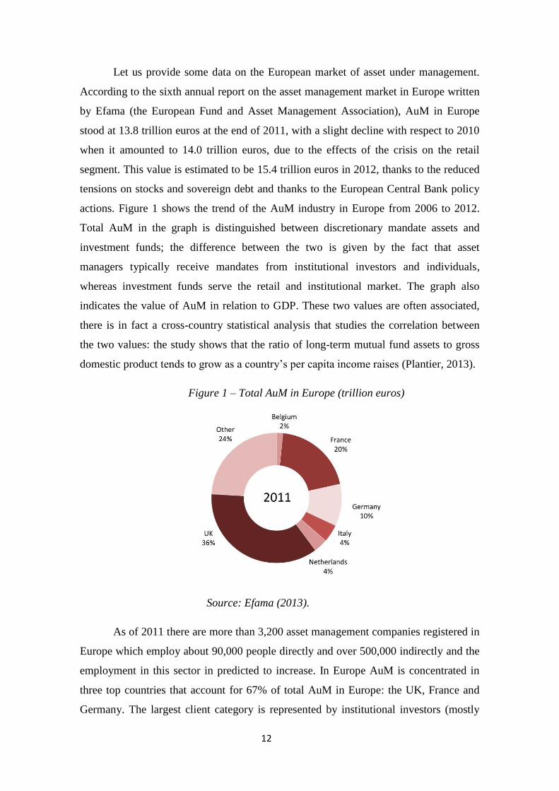
Let us provide some data on the European market of asset under management.
According to the sixth annual report on the asset management market in Europe written
by Efama (the European Fund and Asset Management Association), AuM in Europe
stood at 13.8 trillion euros at the end of 2011, with a slight decline with respect to 2010
when it amounted to 14.0 trillion euros, due to the effects of the crisis on the retail
segment. This value is estimated to be 15.4 trillion euros in 2012, thanks to the reduced
tensions on stocks and sovereign debt and thanks to the European Central Bank policy
actions. Figure 1 shows the trend of the AuM industry in Europe from 2006 to 2012.
Total AuM in the graph is distinguished between discretionary mandate assets and
investment funds; the difference between the two is given by the fact that asset
managers typically receive mandates from institutional investors and individuals,
whereas investment funds serve the retail and institutional market. The graph also
indicates the value of AuM in relation to GDP. These two values are often associated,
there is in fact a cross-country statistical analysis that studies the correlation between
the two values: the study shows that the ratio of long-term mutual fund assets to gross
domestic product tends to grow as a country‘s per capita income raises (Plantier, 2013).
Figure 1 – Total AuM in Europe (trillion euros)
Source: Efama (2013).
As of 2011 there are more than 3,200 asset management companies registered in
Europe which employ about 90,000 people directly and over 500,000 indirectly and the
employment in this sector in predicted to increase. In Europe AuM is concentrated in
three top countries that account for 67% of total AuM in Europe: the UK, France and
Germany. The largest client category is represented by institutional investors (mostly
13
insurance companies and pension funds) that act on behalf of households and they
account for 75% of total AuM in Europe.
1.2.2 The asset management market in Italy
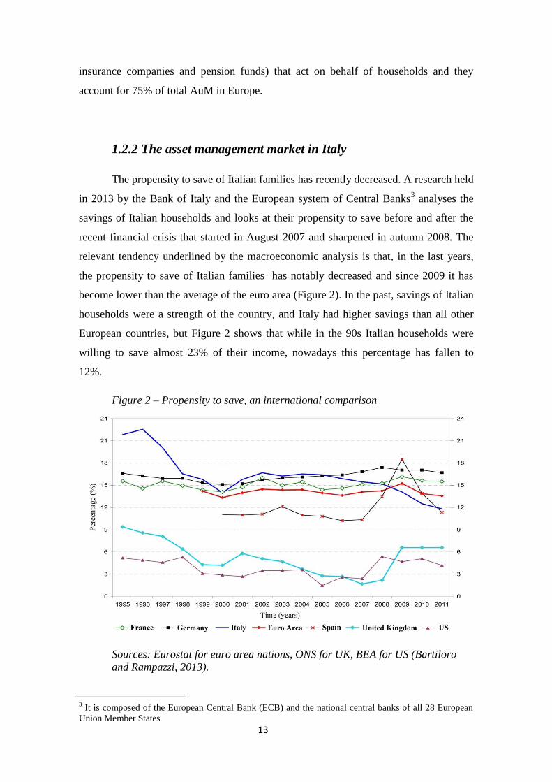
The propensity to save of Italian families has recently decreased. A research held
in 2013 by the Bank of Italy and the European system of Central Banks3 analyses the
savings of Italian households and looks at their propensity to save before and after the
recent financial crisis that started in August 2007 and sharpened in autumn 2008. The
relevant tendency underlined by the macroeconomic analysis is that, in the last years,
the propensity to save of Italian families has notably decreased and since 2009 it has
become lower than the average of the euro area (Figure 2). In the past, savings of Italian
households were a strength of the country, and Italy had higher savings than all other
European countries, but Figure 2 shows that while in the 90s Italian households were
willing to save almost 23% of their income, nowadays this percentage has fallen to
12%.
Figure 2 – Propensity to save, an international comparison
Sources: Eurostat for euro area nations, ONS for UK, BEA for US (Bartiloro
and Rampazzi, 2013).
3 It is composed of the European Central Bank (ECB) and the national central banks of all 28 European
Union Member States
14
Italian asset management legislation is subject to the TUIF (Testo Unico delle
disposizioni in materia di Intermediazione Finanziaria) and to the regulations issued by
the Italian security and stock exchange commission, e.g. the Consob (Commissione
Nazionale per le Società e la Borsa) and the Bank of Italy.
KPMG Advisory4 held a research in 2012 on asset management in Italy. The
research was conducted with the help of the top management of 30 operators that work
in the Italian asset management market (they represent almost 75% of the Italian AuM),
in order to study the recent trends, orientations and drivers that trace the development of
this sector. This paragraph makes use of this research to focus on some important topics.
As reported by KPMG Advisory savings accumulated by Italian private
investors in 2010 are about 50 billion euros, and the wealth of Italian families, net of
monetary liabilities, is equal to 8.600 billion euros, the 40% of which is represented by
financial activities (about 3.200 billion euros). However, Italian households do not make
great use of asset management: only 6% of the portfolio of financial activities is devoted
to mutual funds, while 30% of wealth is liquid (cash, bank deposits and postal deposits).
Furthermore, even pension funds, complementary pensions and financial/insurance
products represent a small portion in the financial portfolio of Italian households (19%
of the total of financial activities)5. Nonetheless, the asset under management market in
Italy is expected to grow. This is due to demographic factors like the extension of the
average length of life of the Italian population but also to the recent reforms taken by
the Italian government on the pension system that are reducing Social security. As a
consequence of this, Italian households will probably tend to favor complementary
pensions and long term investment.
The asset management market experienced many changes in the last years, with
the birth of new financial instruments and new ways of distribution. It mostly developed
in the last decade, but it recently faced several slowdowns due to the financial crisis, the
competition of alternative products, asymmetries of the tax system and the loss of
confidence of investors because of the unstable financial and economic situation. As of
May 2013, the Italian market of asset management has a value of 1.264 billion euros but
it has great potential to grow. The sector of asset management should promote savings
devoted to Social security and at the same time it should lead the investments to finance
4 KPMG Advisory S.p.a. is an Italian society and is part of the KPMG network.
5 All the data are taken from the Bank of Italy.
15
the growth of the industrial apparatus in Italy and the development of the domestic
market. KPMG Advisory put strength on this market for its strategic role in the
development of the country. Nonetheless, it is clear that the asset management sector
can develop only with a proper financial education of investors, together with a set of
clear and simple regulations, and with the creation of investment solutions that suit new
investors needs. It is necessary to enrich the offer of services of advisory addressed to
the single client, and to augment the transparence of information of the sector.
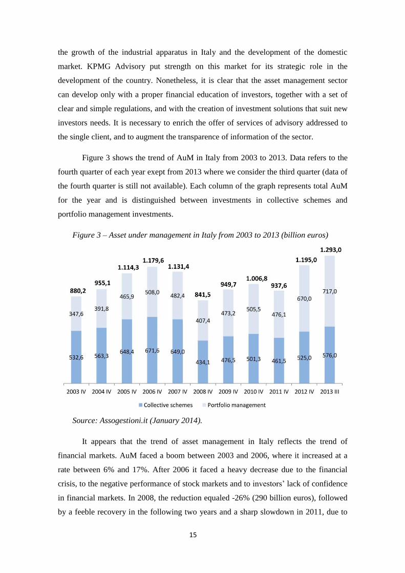
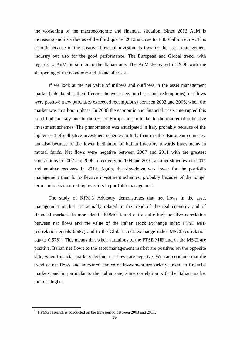
Figure 3 shows the trend of AuM in Italy from 2003 to 2013. Data refers to the
fourth quarter of each year exept from 2013 where we consider the third quarter (data of
the fourth quarter is still not available). Each column of the graph represents total AuM
for the year and is distinguished between investments in collective schemes and
portfolio management investments.
Figure 3 – Asset under management in Italy from 2003 to 2013 (billion euros)
Source: Assogestioni.it (January 2014).
It appears that the trend of asset management in Italy reflects the trend of
financial markets. AuM faced a boom between 2003 and 2006, where it increased at a
rate between 6% and 17%. After 2006 it faced a heavy decrease due to the financial
crisis, to the negative performance of stock markets and to investors‘ lack of confidence
in financial markets. In 2008, the reduction equaled -26% (290 billion euros), followed
by a feeble recovery in the following two years and a sharp slowdown in 2011, due to
16
the worsening of the macroeconomic and financial situation. Since 2012 AuM is
increasing and its value as of the third quarter 2013 is close to 1.300 billion euros. This
is both because of the positive flows of investments towards the asset management
industry but also for the good performance. The European and Global trend, with
regards to AuM, is similar to the Italian one. The AuM decreased in 2008 with the
sharpening of the economic and financial crisis.
If we look at the net value of inflows and outflows in the asset management
market (calculated as the difference between new purchases and redemptions), net flows
were positive (new purchases exceeded redemptions) between 2003 and 2006, when the
market was in a boom phase. In 2006 the economic and financial crisis interrupted this
trend both in Italy and in the rest of Europe, in particular in the market of collective
investment schemes. The phenomenon was anticipated in Italy probably because of the
higher cost of collective investment schemes in Italy than in other European countries,
but also because of the lower inclination of Italian investors towards investments in
mutual funds. Net flows were negative between 2007 and 2011 with the greatest
contractions in 2007 and 2008, a recovery in 2009 and 2010, another slowdown in 2011
and another recovery in 2012. Again, the slowdown was lower for the portfolio
management than for collective investment schemes, probably because of the longer
term contracts incurred by investors in portfolio management.
The study of KPMG Advisory demonstrates that net flows in the asset
management market are actually related to the trend of the real economy and of
financial markets. In more detail, KPMG found out a quite high positive correlation
between net flows and the value of the Italian stock exchange index FTSE MIB
(correlation equals 0.687) and to the Global stock exchange index MSCI (correlation
equals 0.578)6. This means that when variations of the FTSE MIB and of the MSCI are
positive, Italian net flows to the asset management market are positive; on the opposite
side, when financial markets decline, net flows are negative. We can conclude that the
trend of net flows and investors‘ choice of investment are strictly linked to financial
markets, and in particular to the Italian one, since correlation with the Italian market
index is higher.
6 KPMG research is conducted on the time period between 2003 and 2011.
17
KPMG also studied the correlation of net flows with the Italian real economy
and found out a positive correlation with the Italian GDP (correlation equals 0.489).
Even if the correlation is less significant than the one linked to financial markets, it
shows that the investment choice of Italian investors is also related to the real economy.
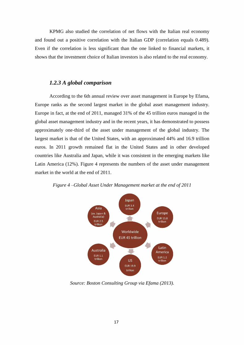
1.2.3 A global comparison
According to the 6th annual review over asset management in Europe by Efama,
Europe ranks as the second largest market in the global asset management industry.
Europe in fact, at the end of 2011, managed 31% of the 45 trillion euros managed in the
global asset management industry and in the recent years, it has demonstrated to possess
approximately one-third of the asset under management of the global industry. The
largest market is that of the United States, with an approximated 44% and 16.9 trillion
euros. In 2011 growth remained flat in the United States and in other developed
countries like Australia and Japan, while it was consistent in the emerging markets like
Latin America (12%). Figure 4 represents the numbers of the asset under management
market in the world at the end of 2011.
Figure 4 –Global Asset Under Management market at the end of 2011
Source: Boston Consulting Group via Efama (2013).
18
1.3 Mutual funds
1.3.1 Mutual funds definition
A mutual fund is a trust that pools money collected from many investors for the
purpose of investing in securities such as stocks, bonds, money market instruments and
other assets. The portfolio of a mutual fund is very diversified and is run by a
professional money manager or, in some cases, a management team, with the aim of
producing capital gain and income for the fund‘s investors. The manager is
compensated by a fee directly deducted from the portfolio.
The manager follows a specific investment objective that is indicated in the fund
contract and decides what types of securities to purchase according to this objective.
Each mutual fund is a separate company and since the mutual fund corporation or trust
is owned by its individual shareholders, it is the shareholders and not the asset
management company who bear the fund‘s investment risk. Besides, the fund‘s assets
are kept by an independent third party, typically a bank or trust company, in order to
protect shareholders from theft by management.
The fund shareholders have equal rights and they participate to the fund returns
and losses with respect to the number of shares held. Mutual funds are in fact divided in
units (the shares) that are subscribed to investors and that grant equal rights. The
numerical value of the shares subscribed by the investor gives the measurement of his
participation to the fund.
The capital of the fund is separated by law from the capital of the asset
management company and from that of the single participants. This characteristic
entails an important consequence: creditors of the asset management company cannot
satisfy their credits with the capital of the fund and so they cannot compromise the
investors rights.
The UCITS Directive in 1985 gave another definition of ‗investment funds‘ as:
―Vehicles the sole objective of which is the collective investment in transferable
securities of capital raised from the public and which operates on the principle of risk
spreading‖ (Directive 85/611/ECC).
19
1.3.2 Main actors in the market of mutual funds
A mutual fund works well if there are four main subjects:
the management company;
investors;
the bank as an independent custodian;
distributors.
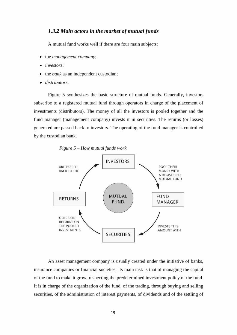
Figure 5 synthesizes the basic structure of mutual funds. Generally, investors
subscribe to a registered mutual fund through operators in charge of the placement of
investments (distributors). The money of all the investors is pooled together and the
fund manager (management company) invests it in securities. The returns (or losses)
generated are passed back to investors. The operating of the fund manager is controlled
by the custodian bank.
Figure 5 – How mutual funds work
An asset management company is usually created under the initiative of banks,
insurance companies or financial societies. Its main task is that of managing the capital
of the fund to make it grow, respecting the predetermined investment policy of the fund.
It is in charge of the organization of the fund, of the trading, through buying and selling
securities, of the administration of interest payments, of dividends and of the settling of
20
account balances. It constantly monitors the development of the fund and selects stocks
with the aim of keeping the portfolio at an optimal quality level.
Shortly, it operates in this way:
1. It studies financial markets in general through economic variables (GDP,
inflation, interest rates) to define the background tendency that might influence
the market in the medium-long term. This is defined as the macroeconomic
analysis.
2. It studies each listed company through an analysis of balance sheets, periodic
publications on financial websites and ratios (to calculate for example liquidity
and returns), with the aim of getting an evaluation of the society and an estimation
of the future trend of each company‘s price. This is defined as the fundamental
analysis.
3. It decides how to split the capital among the macro categories of securities (like
stocks, bonds, short term investment instruments and hedging instruments),
among geographic areas (like Italy, Europe, America and Pacific), among
commodities sectors (like chemical, banks and real estate). This step is called
asset allocation and this activity is defined both studying the macroeconomic
scenario but also respecting the policy of the fund.
4. It selects the single stocks to buy (or sell) after a meticulous study of each stock.
This is called stock picking activity.
5. Finally, it decides the best moment to buy or sell a group of stocks or single
stocks after a technical analysis that makes wide use of statistics and estimates the
trends of the market in general and some specific financial instruments. This is the
activity of market timing that many experts of financial markets consider to be
fundamental for the success of the fund.
Investors are the owners of the fund, since the fund represents their collective
capital. Each subscriber to the fund invests a sum according to his possibilities: the sum
of participation might be significant or modest. Nonetheless, the weight of the
investment has no matter in terms of rights: all the investors have the same rights and all
the investors benefit of the same performance realized by the fund in a certain time
frame. So, if the fund performed a 10% increase in one year, all the investors that
owned the shares of the fund since the beginning of the year will get a return of 10% at
the end of the year, whether they invested 1.000 or 100.000 euros.
21
The independent custodian bank is in charge of the administration of the capital
of the fund and it oversees on the asset manger operations to make sure that they are in
line with the laws and regulation of the fund. It also keeps in custody the stocks and
liquidity of the fund, it regulates the operations of the asset manager and the credit of
interest payments. This is a guarantee for the investor because the money is in the
custody of a third party and not of the asset manager society. The Italian regulation of
the bank custodian is even stricter than in other countries and it is the form of
investment most protected by law.
Fund distributors manage the subscription procedures but also help investors in
their investment choices. They act as a wholesaler if they sell shares to securities dealers
who then sell to investors, or they might deal directly with the public as a retailer (De
Marchi and Roasio, 1993).
1.3.3 The scenario of development of mutual funds
The popularity of mutual funds investing is undeniable. Fredman and Russ
write: ―Making money is in vogue these days. […] And investing is a big part of the
money-making equation. Cash you don‘t need now can be put to work –to finance
everything from child‘s education or a new home purchase to your retirement‖. And
mutual funds perfectly suit this statement.
Mutual funds grew explosively almost all around the world during the 1990s. In
the United States, mutual funds total net asset grew from USD 1.6 trillion in 1992 to 5.5
trillion in 1998, with an average annual rate of growth of 22.4%. The rapid growth of
mutual funds in the US is due to the increase in households‘ ownership of mutual funds.
The percentage of US households owning mutual funds grew from 6% in 1980 to 27%
in 1992, to 44% in 1998 and to a peak of 52% in 2001, before falling back to 49.6% in
2002. This trend is the consequence of a positive orientation of investors towards the
financial system: the strong performance of equity and bond markets, the increasing
globalization of finance and the development of capital markets lead investors to
increase confidence towards market integrity, liquidity and efficiency. Another
phenomenon that contributed to the popularity of mutual funds is the demographic
aging of the population of most high and middle-income countries and the consequent
22
growth of a segment of investors that look for financial instruments that grant long-term
return like mutual funds (Fernando et al, 2003).
A very similar trend was experienced by the 15 countries of the European
Union, where total net asset grew from USD 1 trillion in 1995 to 2.6 trillion in 1998,
with an average annual growth rate of 17.7% (Fernando et al, 2003). Data of EFAMA
confirm the success of the market of UCITS7.
Concerning Italy, mutual funds expanded between 1995 and 2000, when the
number of mutual funds grew from 400 to 800 and money invested in mutual funds
went from 120 trillion of Italian liras to 750 trillion. Their popularity started with the
reduction of interest rates of Italian Treasury Bonds (BOT, Buoni Ordinari del Tesoro),
which lead investors to look for investment instruments different from the traditional
ones like the BOT, Treasury Bonds with long term maturity (BTp) and Treasury Credit
Certificates (CcT). Moreover, it started to develop the concept of real diversification
even among households. Whereas for many years investors diversified buying fixed rate
BTp, variable rate CcT and some stocks, with the birth of mutual funds, people started
to understand that the globalization of financial markets required to further diversify and
they considered the possibility to include in the portfolio securities of different business
areas but also of different geographic areas. In this scenario, the number of financial
products grew all over the world, competition between banks and other financial
intermediaries sharpened and the financial markets became more and more global
(Bartiloro and Rampazzi, 2013).
The phenomenon characterized also developing countries in the Asia-Pacific
world and so it follows that all the four broad regions (the United States, Europe, Asia
Pacific and the rest of the world) faced a strong growth in the market of mutual funds.
Global assets in mutual funds in fact increased from 4 trillion dollars in 1993 to 28.9
trillion dollars in September 2013 (Plantier, 2013).
To conclude we sum up the main factors responsible of the phenomenon of
development of mutual funds on the global basis.
7 UCITS (Undertakings for collective investment in transferable securities) are a set of European
Directives giving European passport to a financial product. As a consequence, a fund authorized by one
member state could operate with no limits in Europe. In reality, however, every State established a set of
rules to protect its local asset management. established to allow to collective investment schemes to
operate freely around Europe unifying the legislation and
23
1. Households‘ increased demand to invest in professionally managed investment
products to indirectly access capital markets. By pooling the investment of many
individuals in fact mutual funds allow to household investors to invest in a
diversified exposure to securities that they might individually find too costly or
unattainable.
2. The creation of an appropriate regulation of capital markets at the mutual fund
level to provide an adequate disclosure and to limit potential conflicts.
3. The increased availability of deep and liquid capital markets. There is strong
evidence that the size of a country‘s capital market is correlated with the size of
the mutual fund industry.
4. The availability of a large common market where mutual funds can be bought and
sold, this is confirmed by the fact that the greatest market of mutual funds is that
of the U.S. (that is by nature a common market) and the European, which are both
large common markets.
5. Capital market returns. Even if in the short-run returns on the stock and bond
market can vary significantly from year to year, in the long-run returns tend to be
favorable. Thanks to mutual funds, investors can access these favorable returns
through a diversified and professionally managed product.
6. The economic development of a country. This is fundamental since mutual funds
are considered as a superior good (Fernando et al., 2003) and so ownership of
mutual funds increases with households‘ income.
7. Demographic changes that are making retirement schemes increasingly
unsustainable. Retirement schemes were created when a large number of workers
supported a smaller number of retirees. But the support ratio, that is the measure
of the number of working-age people relative to those of retirement age fell
sharply. By 2050, the support ratio in Japan, Australia, US, Germany, UK, France,
is expected to be about 2.2 workers per retiree, compared to the 7.8 workers per
retiree in 1950. This leads individuals to shift to private investments to finance
their retirement.
8. The introduction of defined contribution (DC) plan systems. Changes in
demography led states to adopt (DC) plan systems which make great use of
mutual funds. DC plan systems differ around the world: in the US the level of
contribution is chosen by employees and employers may match part of the
contribution of the employees; in others, like Chile and Australia the government
24
establishes a minimum contribution and allows for additional contributions above
the minimum level. Despite this, the important thing here is that these systems
allow participants to choose investment, including investment in mutual funds
(Plantier, 2013).
1.3.4 Mutual funds in Italy
The first Italian experience with mutual funds dates back to 1960, when it
appeared the first Italian-Luxembourg fund called Interitalia, that was domiciled in
Luxemburg but created by the Italian bank Banco Ambrosiano. The fund was not
domiciled in Italy since there was not a norm that regulated mutual funds in Italy. The
choice of Luxemburg instead of other countries was due to its favorable taxation (De
Marchi and Roasio, 1999). A law of 1983 made it possible to buy funds of Luxemburg
legislation and after that date the share of Italian households‘ financial assets invested in
mutual funds grew steadily.
It is interesting to consider the results of a research conducted by McKinsey
Global Institute that makes a comparison on the elements taken into consideration when
investing in funds in Italy and in the US8. In Italy, the most relevant element influencing
the choice of mutual funds is the brand of the selling society, followed by: capital
guaranteed (we consider capital guaranteed as a low risk/return profile instead of a real
guarantee on the money invested), clear information on the risk, clear information on
the performance, the simplicity of the service, the liquidity of the investment and, at the
last, the performance. The result of the research in the US market is totally different:
performance is at the top of the list, followed by a simple and without problem service,
advice in the fund selection, low commissions, brand, availability of the service twenty-
four hours a day, advise on the asset allocation and wide availability of products.
The difference between the two lists is notable, in particular considering the
positioning of the performance of the fund. Italian investors appear to be interested in
elements that are not a guarantee of a good result of the investment, such as the brand.
American investors instead, are interested in elements linked to the financial success of
the investment, such as low commissions, advice on the asset allocation and variety of
8 The research is discussed by Liera, 1999.
25
products offered. One of the main reasons of this difference might be explained by the
different ways of distribution of mutual funds in the two countries. In Italy, mutual
funds are sold by networks of financial advisors, by banks, directly by the asset
management company or through the internet, with certain restrictions. In the US,
instead, the distribution does not occur under the advisory of the bank that sells its own
funds, but under the advisory of an independent expert (De Marchi and Roasio, 1999).
1.3.5 Advantages of mutual funds
Mutual funds are extremely flexible instruments that are totally adaptable to the
specific request of each investor. The mechanism of investment, the rules of
participation and interest payments are the same for each investor, but the way in which
a fund is used to reach certain objectives is absolutely specific to each individual.
Thanks to their organization and structure, they offer several advantages.
First of all mutual funds allow even to small household investors to get close to
stock markets: the subscription to a mutual fund in fact requires a small initial sum.
Moreover, investors have the possibility to accumulate money on, for example, a
monthly basis; with this mechanism they accumulate capital through years without a
huge sacrifice, because they periodically take a small amount of money from their
monthly savings and invest it to make it grow.
Moreover, the portfolio of each fund is very diversified. Mutual funds invest in a
dozen or so stocks up to several hundred in larger portfolios and as a consequence they
contain very little company specific risk. To sum up, they allow a diversification that a
small investor alone could never reach. Diversification is always the basis of a good
investment, and it is even more important now that financial markets are global and it is
difficult to reach full information about foreign investments.
Mutual funds popularity grew among small investors also because of the ease to
convert the investment in liquidity. Mutual funds shares can be purchased but also
redeemed quickly. The Italian legislation of mutual funds requires asset management
companies to redeem shares to investors within 15 days from the request. Further,
money can be efficiently switched between, say, a stock and a money market fund at
little or no-cost.
26
Since their birth, mutual funds have always guaranteed a quite high return in the
medium and long run. They are not an instrument for speculation in the short term but
an instrument that invests and maximizes results in the long term. It is also relevant to
say that, even if it is possible to experience a loss if the fund‘s holding declines in price,
the probability of fraud, scandal or bankruptcy involving the fund‘s management
company is very small. This is possible because the investment risk is shifted to
shareholders, and because the legal structure and regulation is very strict. Moreover the
management company and other affiliated parties cannot undergo certain types of
transactions, so the risks faced in mutual funds arise only from fluctuations in the stock
or bond market but not from foul play. As a consequence mutual funds are generally
seen by investors as a safer investment compared to other forms of investment
(Fredman and Wiles, 1993).
Also, investments in mutual funds are guaranteed lower taxation. In Italy, Italian
law 461/97 granted a substitute tax of 12.5% on returns of the fund for Italian and
Luxembourg funds. The recent legislative decree number 225 of 29th
December 2010
established that from the 1st of July 2011, taxation of the returns is shifted from the fund
to the single subscribers of the fund. This adjustment was made to recognize to Italian
and Luxembourg funds the same taxation currently in use in all the other member States
of the European Union (Assogestioni, 2011)9.
Lastly, mutual funds offer the possibility to invest in a low cost diversified
portfolio managed by a skilled, experienced professional manager. Managers are
periodically judged by the total return they generate and those who do not produce are
replaced, since the choice of the best management is one of the key aspects of the
success of a fund.
Italian mutual funds regulation is characterized by great transparency, there is no
investment instrument in Italy that has similar regulation in terms of transparency. The
Italian Security and Exchange Commission CONSOB (Commissione Nazionale per le
Società e la Borsa) obliges mutual funds to publish a documentation that provides
detailed information on the working mechanisms of the fund. The two main documents
9 For ten years the asset management market experienced a flow from investments in Italian mutual funds
towards mutual funds of the European Union. The main cause was the unfavorable fiscal treatment of
Italian mutual funds. In fact, before 2011, Italian taxation of returns of mutual funds was in charge of the
fund, without regard to the fact that investors collected the returns or not, while in the rest of the
European Union the returns of harmonized funds were taxed directly to the subscriber when they actually
got the returns (Assogestioni, 2011).
27
in the Italian legislation of mutual funds are the prospectus and the document of
regulation of the fund management, together with other documentation like the double
entry bookkeeping and the semi-annual and annual report.
The composition of the prospectus is fixed and easy to read and understand. The
main aim of the prospectus is that of granting to the subscriber an easier comparison
between the fund he is subscribing to and other mutual funds, and to provide all the
information needed both for his prevention and knowledge. The prospectus answers
most of the questions about the fund. It contains information on the legal status of the
fund, on the independent custodian (usually a bank), on distributors, on the main
characteristics of the fund and on the subscription policies. It also describes the
objectives of the investment, the investment strategy, the investment risks, transaction
costs and ongoing expenses, the benchmark, taxation and financial history and
explanations on how to purchase and redeem shares. The document of regulation of the
fund management instead is the document through which the management society
creates the fund and it is the document that the subscriber undersigns to state that he is
aware of the conditions and characteristics of the fund.
1.4 Categories and costs of mutual funds and life insurance plans
1.4.1 Mutual funds classification in Italy
Mutual funds classification in Italy is currently held by Assogestioni, the
representative association of the Italian investment management industry. Assogestioni
represents most of the Italian and foreign investment management companies operating
in Italy, as well as banks and insurance companies involved in investment management,
including pension schemes, with the main aim of fostering the investment management
industry in Italy. The classification is intended to make the functioning of mutual funds
clearer and to give the right placement to funds with different characteristics as a useful
instrument for all the actors in the market of funds.
Assogestioni classification came in force on July 1st, 2003; its basic principle is
that of looking at the final investor, the so called ―weak party‖, and it takes his point of
view respecting the basic principles of financial markets. The classification should
allow investors to understand immediately and in an easy way the most evident risky
28
factors of investing in funds and it should induce them to read carefully the prospectus
and all the documents that are part of the contract of investment. It is not to be
considered as an instrument to make an analysis on risk and return of each single
investment.
The classification is precise and is based on objective parameters. The first
division of mutual funds into five macro areas is on the base of the portfolio
composition. We now list mutual funds according to this classification in a decreasing
order, on the base of the percentage of stocks held in the portfolio:
1. Stock or equity funds;
2. Balanced funds;
3. Bond funds;
4. Money market funds;
5. Flexible funds.
Equity funds invest at least 70% in stocks, balanced funds invest in stocks only
in a percentage that goes from 10 to 90, bond funds and money market funds cannot
invest in stocks, and flexible funds do not have any constraint on the percentage of
stocks to keep in the portfolio. Let us now describe in more detail the composition and
basic features of each category.
Stock or equity funds invest in common stocks that represent ownership equity in
corporations. Thanks to trading operations, these funds grant higher returns than other
funds, but also higher risk. They are generally characterized by a main investment of
70% of the portfolio invested in stocks, and a residual investment of 30% invested in
bonds or money market instruments. Generally, the specific sector or geographic area in
which the fund is invested gives the name to the fund. According to this, they can be
further divided into: equity fund Italy, Euro Area, Europe, America, Pacific, Emerging
Markets, Country, international, energy and raw materials, industrials, common goods,
health, finance, information technology, telecommunication, advertisement, other
sectors and other specializations. Mutual funds that belong to the categories equity Italy,
Euro area, Europe, America, Pacific and emerging markets are characterized by the
main investment in stocks invested in the specific geographic areas of definition.
Mutual funds of each State are characterized by the main investment in the State defined
by the regulation; mutual funds that belong to the other sector categories are determined
29
by the main investment invested in stocks belonging to one or more of the sectors
specified by the Global Industry Classification (GICS). Usually the sector
categorization prevails on the geographic one.
Balanced funds invest in bonds and stocks. They can be further differentiated in
balanced equity funds (with stocks in a proportion between 50% and 90%), balanced
funds (with stocks in portfolio between 30% and 70%) and balanced bond funds (with
stocks in portfolio between 10% and 50%).
Bond funds invest especially in fixed income or debt securities. Different kind of
bonds can be included such as high-yield bonds, junk bonds, investment-grade
corporate bonds, government and municipal bonds. The classification of bond funds is
defined according to the combination of risky factors that we define with:
Market risk:
Currency denomination: euro, dollar, yen or other currencies;
Portfolio duration.
Credit risk:
Issuer‘s jurisdiction: developed or emerging markets;
Type of issuer: State or firm;
Credit merits: investment grade or high yield.
Assogestioni defines several specialized categories among bond funds:
short/medium/long term government bond in euro area, euro corporate investment grade
bond, euro high yield bond, short/medium/long term government bonds in dollars,
dollar corporate investment grade bonds, dollar high yield bond, international
government bond, international corporate investment grade bond, international high
yield bond, yen bond, emerging market bonds, other specialized bonds. Non specialized
bonds are mixed bonds and flexible bonds.
Money market funds invest in bonds and money market instruments, mostly
short-term financial instruments like Treasury Bonds, certificates of deposit and long
term bonds with a residual life not greater than six months. The main feature of this
category is the level of liquidity of the investment and the necessity to continuously
switch the composition of the portfolio to profit from the negotiation. According to
30
Assogestioni, financial instruments in the portfolio cannot have a rating smaller than A2
(Moody‘s), A (S&P) or an equivalent rating given by an independent rating agency, and
the duration of the portfolio should be smaller than six months. Liquidity funds differ
according to the currency of emission of the securities in the fund: euro money market
funds, US dollar money market funds, yen money market funds and other currencies
money markets.
Finally, flexible funds are characterized by the fact that they do not follow a rigid
investment scheme, they might change their investment strategies as they see fit. This
means that they do not stick to one particular strategy as other categories of funds do,
but they privilege investments in stocks or bonds according to market perspectives.
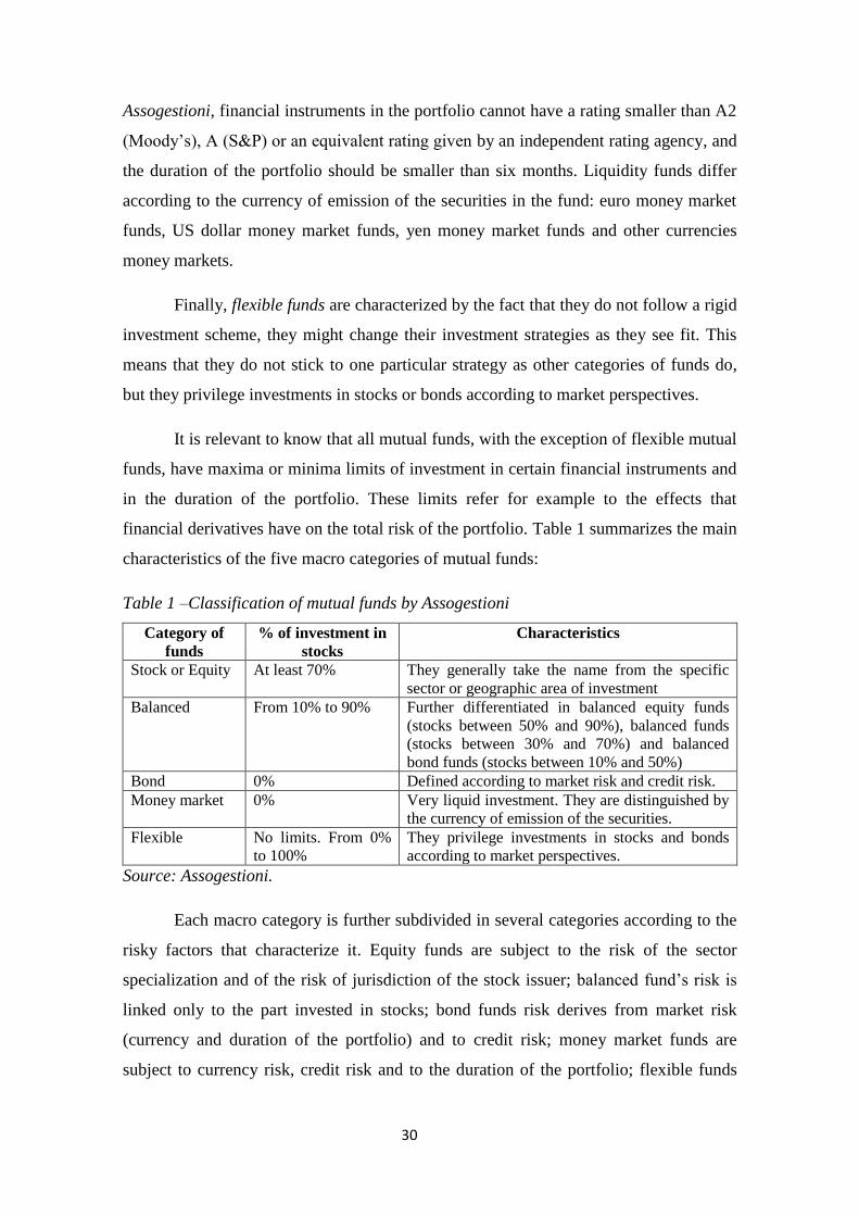
It is relevant to know that all mutual funds, with the exception of flexible mutual
funds, have maxima or minima limits of investment in certain financial instruments and
in the duration of the portfolio. These limits refer for example to the effects that
financial derivatives have on the total risk of the portfolio. Table 1 summarizes the main
characteristics of the five macro categories of mutual funds:
Table 1 –Classification of mutual funds by Assogestioni
Category of
funds
% of investment in
stocks
Characteristics
Stock or Equity At least 70% They generally take the name from the specific
sector or geographic area of investment
Balanced From 10% to 90% Further differentiated in balanced equity funds
(stocks between 50% and 90%), balanced funds
(stocks between 30% and 70%) and balanced
bond funds (stocks between 10% and 50%)
Bond 0% Defined according to market risk and credit risk.
Money market 0% Very liquid investment. They are distinguished by
the currency of emission of the securities.
Flexible No limits. From 0%
to 100%
They privilege investments in stocks and bonds
according to market perspectives.
Source: Assogestioni.
Each macro category is further subdivided in several categories according to the
risky factors that characterize it. Equity funds are subject to the risk of the sector
specialization and of the risk of jurisdiction of the stock issuer; balanced fund‘s risk is
linked only to the part invested in stocks; bond funds risk derives from market risk
(currency and duration of the portfolio) and to credit risk; money market funds are
subject to currency risk, credit risk and to the duration of the portfolio; flexible funds
31
instead do not have a type of risk that can be generalized for the category because they
do not follow a fixed pattern.
As already said, the classification of Assogestioni is based on specific politics of
investment and it is created with the aim of helping investors to understand mutual
funds. To supplement this categorization, Assogestioni provides the definition of some
qualifications proper to the politics of investment in mutual funds, that help to define
the mechanisms of some funds but that are external to the basic classification. This
means that these features are independent from the previously described classification,
they only represent a supplemental description that is important to know. Before listing
these characteristics, there are two important conditions to keep in mind: first, the fund
denomination must contain the conditions that recall the qualification that the asset
manager declares; second, the fund regulation should illustrate with precision the
constraints applied to the policy of investment that justifies the declared qualification of
the fund.
First qualification is that of ethic funds. The politic of investment of an ethic
fund denies the purchase of certain stocks and privileges the purchase of others
according to the fund ethical criteria. This means that ethic funds do not invest with the
sole criterion of maximizing the return from the investment but also respecting ethical
principles that are defined by the corporate governance of the fund. Usually, the
decision of which stocks to buy is linked to the social effects that the activity of the
issuer corporation has. Criteria can be ―positive‖ or ―negative‖: funds that follow
negative investment criteria do not invest in stocks whose issuing firm violates some
moral principles (for example firms that produce weapons or firms in States that violate
human rights); funds that follow positive criteria, instead, invest in firms that result to
be the best according to a certain social criterion (for example a firm that has the lower
level of pollution in its sector) or in firms with specific ethical objectives (the protection
of the environment).
Another qualification is that of capital protection. Capital protection funds
follow a policy of investment where the objective is the protection of the value of the
investment. They apply quantitative techniques on the management of investment to
limit losses. No more guarantees are granted other than the fact that the value of the
investment do not go under the level of protection. The value of the investment depends
on a quantity linked to the value of the share of the fund. It is important to notice that
32
capital protection funds have guaranteed capital but do not have certain return. Capital
guarantee funds instead grant to each subscriber, independently from the results of the
fund, the return of a predetermined percentage of the capital placed in the fund at
maturity. In these last two types of funds any losses experienced by the underlying
investments are absorbed by the fund company, this is why the majority of the fund
capital is invested in very conservative securities. As a consequence of trying to limiting
losses through investments in risk-free securities, these funds offer a very low rate of
return.
The last qualification described by Assogestioni is that of index funds. Index
funds policy of investment has the objective of duplicating the risk/return profile of a
market index.
1.4.2 Other categories of mutual funds
There are other classifications of mutual funds different from that of
Assogestioni and based on other parameters. Before talking about some of these
categories that are of interest for the aim of our analysis, let us clarify a point.
In Italy, the two broad categories of investment funds are basically mutual funds
and SICAV, e.g. the acronym for French Société d’investissement à capital variable.
The difference between the two is the fact that mutual funds have a distinct and
independent capital formed by the money invested by the subscribers and it is managed
by an asset management society, SICAV instead are societies whose subscribers are
shareholders with the relative rights, like the right to vote. The activity of asset
management in a mutual fund is usually delegated to an asset management company
while in a SICAV it is usually conducted by a team of managers of the SICAV itself.
Sometimes even the SICAV delegates the management of the whole portfolio or of a
part of it to an external asset manager. In this case, the board of directors of the SICAV
defines to the asset manager the objectives of the fund and controls how the asset
manager works. SICAV and asset management societies are the only two organizations
that can exercise the activity of management in collective investment schemes. In Italy,
they can operate only with the authorization of the Bank of Italy (and indirectly of the
Consob). In practice, mutual funds and SICAV work for the same economic purpose
33
that is the collective management of the money collected from the investors. This is
why, for the intent of our analysis, we will talk about mutual funds and SICAV
interchangeably.
Mutual funds can be distinguished according to the diversification of their
portfolio. Diversified funds invest in corporations that belong to different economic
sectors and to different geographic areas, specialized funds instead invest in societies
that belong to the same business sector or to the same geographic area. Examples of
specific business sectors are the pharmaceuticals, biotechnologies and common goods.
Another categorization is based on the technical subscription features. Investors
can choose to invest in mutual funds through a one-time lump sum investment, a
systematic investment plan or a systematic transfer plan. A one-time lump sum
investment requires that investors put a lump sum amount and buy mutual fund shares at
once; a systematic investment plan (SIP) is a system that allows to invest a fix amount at
regular intervals in a particular scheme10
. The other modality of investment is the
systematic transfer plan (STP), where the investor invests a lump sum in a scheme and a
small amount at regular intervals in another scheme, allowing to adhere to the asset
allocation suitable for the client and to earn higher returns from the scheme that
performs better.
Depending on their organizational structure, mutual funds can be divided
between closed-end and open-end funds. Closed-end funds are investment societies with
fixed capital, this means that capital cannot change with new subscriptions and
redemptions of shares, and the number of shares outstanding is pre-determined and
cannot change. The only way to augment the number of shares is through an increase in
capital subject to usual procedures of corporations. Closed-end funds shares can be
listed on the stock exchange. Open-end funds, on the contrary, issue new shares to
incoming investors at the current price or net asset value and repurchase or redeem
shares from investors exiting the fund; the redemption takes place in a maximum
predetermined period. The possibility to issue and redeem shares at any time is the main
feature of open-end funds. As a consequence, the net asset value of an open end fund
varies not only according to the financial activities in which it invests, but also
according to the amount of existing shares, that is the number of subscriptions (the
10
A SIP is managed in a way that the investors buy more units when the stock market is down and a
fewer units during an upsurge. This mechanism is also called Rupee cost averaging.

34
investors that invest in the fund) and redemptions (the number of investors that redeem
their shares). Every share must be redeemed at the real value (that means the real value
of the stocks owned, valued at the price of the day in which the redemption is
demanded); as a consequence the number of shares in circulation cannot be prefixed but
varies continuously. The choice of the structure is often functional to the different
politics of investment. Closed-end mutual funds investments are long term and tend not
to be liquid (real estate, credits) since the manager of the fund needs a certain stability
of the fund capital for a certain period of time. Open-end funds instead usually invest in
stocks, bonds and other quoted instruments that can be negotiated in the market. In fact
they do not necessitate a stable capital, since in case of need of liquidity they sell the
stocks of the portfolio.
In Italy, another important criterion of definition of mutual funds is given by the
origin of the fund: there are funds of Italian legislation and funds of foreign legislations,
e.g. constituted in States other than Italy, but sold in Italy. Funds in compliance with the
European Union legislation are called harmonized mutual funds. They are constituted in
the European Union that mostly invest in listed financial instruments. The word
harmonized derives from the fact that they follow the rules and common criteria
required by the European community.
The level of activity of the management of the fund is the discriminating factor
for the distinction between funds under active management and passive management.
The level of activity of a fund is defined by the difference between the return of the
fund and the benchmark. The benchmark11
is the standard used to measure the fund
performance. The more the fund portfolio is close to the benchmark portfolio, the more
the return of the fund is close to the return of the benchmark. In a perfectly passively
managed fund, the fund return and the benchmark return are equal: the fund manager
owns at any time a portfolio equal to that of the fund. Since the benchmark often
corresponds to a stock market index, whether it is an equity market index, a bond
market index or an average of indices, funds with a perfectly passive management are
also defined index-funds (as already seen in Paragraph 1.2.5). An index fund does not
necessarily invest in all the stocks that form the index, they can perform a semi-passive
management choosing a subgroup of stocks that replicate the fund. The management of
an index fund does not require an analytical structure and specific studies of the stocks
11
Definition of ―benchmark‖ in Paragraph 1.5.2; see Chapter 2, Paragraph 2.5 for more details.
35
and financial markets for the asset allocation, an automatic system of conversion is used
for investments; this also makes index funds less costly. Actively managed funds allow a
variety of investments instead of investing in the market and they give the possibility to
follow different strategies of investment. They are more volatile since the fund manager
aims at beating the benchmark and he is willing to undertake higher risks in order to do
that.
Funds of funds are characterized by the fact that they invest in shares of other
funds or SICAV and are non harmonized mutual funds. From the point of view of their
structure and organization they are open-end funds, subject to daily publication of the
value of its shares, and they have some restrictions. Still, the policy of investment of this
instrument should be consistent with the fund objective. Funds of funds can be multi-
brand, if they invest in funds managed by more than one asset manager, or mono-brand,
if they invest in funds of one asset manager, and they have different risk/return profiles.
One of the advantages of this category of funds is the higher level of diversification;
even if certain mutual funds are conceptually close to stock or bond funds, they have
lower idiosyncratic risk12
(De Marchi and Roasio, 1999; Beltratti and Miraglia, 2001;
Santoboni, 2012).
1.4.3 Mutual funds costs
When talking about mutual funds it is always important to keep an eye on fees
and shares that investors incur. These costs pay for expenses sustained by the fund
manager when providing sales services, portfolio management services, fund
administration, subscription to the fund shares, reimbursement and other costs related to
the activity (Anolli, Del Giudice, 2008). Costs might erode the returns if the manager is
not faring well, and high costs exert an even heavier weight when compounded over
many years, in fact even a slight difference in costs can make a big difference if the life
of the investment is quite long. In fact, it is evident that funds with lower costs put more
money working for the investors.
The four basic types of fees or expenses associated with funds are:
12
Definition of ―idiosyncratic risk‖ in Chapter 2, Paragraph 2.3.7.
36
1. Sales charges, that include front-end loads, back-end loads and ongoing asset-
based sales charges. Front-end and back-end loads can be fixed or a percentage
(constant or decreasing). Front-end loads tend to decrease as the capital is put into
the fund, back-end loads instead can decrease, especially according to the length
of adherence to the fund.
2. Ongoing services paid by a fund company to brokers and salespersons for
personal assistance to the clients, that is mainly an investment advice.
3. Ongoing management and administrative costs. These include the costs of the
management of the fund together with those for the custodian and the transfer
agent.
4. Costs associated with the trading of the securities in the portfolio.
Portfolios with no charges in the first two categories are called no-load funds
(Fredman and Wiles, 1993).
In order to understand the reason of costs in mutual funds it is necessary to think
about their functioning. Mutual funds in fact give the opportunity to investors to redeem
shares in every moment, this means that the manager of the fund has to keep a part of its
portfolio in liquidities, in order to guarantee it whenever requested by the investors.
After the request of redemption, the manager of the fund can use the existing liquidity,
but at the same time he has to restore the liquidity to the optimal level selling some
shares of the portfolio.
1.4.4 The binomial insurance-mutual fund
One of the marketing strategies of mutual funds is that of linking the fund with
another product with different characteristics, with the purpose of offering to the
subscriber the synergy of the two operations in one contract. A widely used solution is
that of mixing a financial and insurance instrument together to realize a capital
accumulation through investment plans with the coverage of risk of several life events
(in particular the death or the injury of the subscriber) with one contract. One of the
main reasons of this combination is due to the fact that the market is developing a strong
demand for Social security instruments that grant the commercial success of these
37
integrated products. This combination is the first one to channel mutual funds into a
specific strategy (Santoboni, 2012).
In more detail, the subscriber of the fund, in addition to signing the prospectus
and choosing the formula of investment that he prefers (systematic investment or lump
sum investment), signs a life insurance that insures the capital that he invested in the
fund in a lump sum or the total capital that he will invest through regular investments.
They work in this way: in the case of a lump sum investment, the first insurance
premium is paid simultaneously to the investment and the others are directly taken by
the asset manager firm disinvesting the shares of the fund. In the case of a systematic
investment scheme, the periodic deposits are divided in two parts: one goes into to the
fund to form the capital in little steps, the other one covers the life insurance premium
and the first premium is usually paid together with the first deposit. The length of the
insurance can be decided by the subscriber according to his needs, his age, his
objectives and the sum he wants to deposit. The deposit is tax deductible up to a certain
maximum threshold.
Every investor should be interested in such investing formulas because everyone
should feel the need to benefit from a financial investment linked to an insurance
coverage, since the need of making the money grow and that of protecting the capital
match well together. It would be nonsense to start a systematic investment in a fund
with the risk of stopping it because of the death of the subscriber (and heavy
consequences on the family). The combination of two contracts in one is especially
thought to satisfy the need of protecting the investment for Social security. In Italy, the
problem of social and health care is a hot topic right: with the recent reforms of the
pension system private investors have lost their confidence towards the State and they
are more and more considering investments their Social security (De Marchi and
Roasio, 1999).
1.4.5 Unit linked insurance plan
A type of life insurance plan that is growing popularity is the Unit Linked
Insurance Plan (ULIP). This plan is a goal-based financial solution and combines the
safety of insurance protection with wealth creation: a part of the investment is devoted
38
towards providing life cover while the residual portion is invested in a fund or a mix of
funds that invests in stocks and bonds and the value of the investment changes with the
performance of the fund chosen by the investor. Once decided the amount to invest, the
insurance company deducts some portion of the ULIP premium upfront and the
remaining amount is invested in one or more funds. The mortality and administration
charges are deducted on a periodic basis by cancellation of units, while the ULIP fund
management charges are adjusted from NAV on a daily basis. Say it in another way, the
policyholder purchases units at their NAV but also contributes to another investment
vehicle for the coverage of an insurance policy.
This solution offers higher flexibility, higher liquidity and shorter term bindings.
Flexibility consists also in the possibility to choose the funds among those that the
insurance provider offers and to switch between funds without the necessity to go out of
the plan (Santoboni, 2012).
1.5 Financial markets
1.5.1 Regulated and OTC market
Financial markets are the theater where buyers and sellers trade assets like
equities, bonds, securities and derivatives. Basically, financial markets are used to
match those who want capital with those who have it. Financial markets do their trading
through exchange or through Over-The-Counter markets (OTC). In the first case the
market operates with exchange trading and transactions are coordinated by a centralized
source that links the buyer and the seller. The mechanism of trading on a centralized
system favors the security of transactions and there is very low chance of price
manipulation by mediators. The typical example of an exchange traded market is the
New York Stock Exchange. On the other hand, in over-the-counter markets there is not
a central entity that coordinates trading, there are many mediators with the competence
of linking buyers and sellers with the advantage of having the lower costs of
intermediation possible. The pitfall is that there is no regulation and trading is subject to
fraudulent behaviors by mediators together with price manipulation by competing
mediators. An example of OTC markets are forex trading markets and markets for
buying and selling debt.
39
The efficient market hypothesis (EMH) was formulated by Eugenie Fama in
1970 and it asserts that well organized capital markets are efficient markets and that at
any time, prices fully reflect all available information. In more detail, prices reflect the
information given by financial news, politics, and social and economic events combined
with investors‘ perception. It is then useless to try to beat the market: no investor can
beat and outperform anyone else since they all have the same information, and any
investment approach or strategy would not be successful. Moreover, EMH school
supports the ―random walk‖ of prices: market prices are not predictable but random.
The efficient-market school has been the target of several criticisms. When it
was first publicized it was criticized by words to the effect that ―throwing darts at the
financial page will produce a portfolio that can be expected to do as well as any
managed by professional security analysis‖ (Malkiel, 2003). This statement proves that
despite the great attention and attraction that the idea of efficient markets has
demonstrated in the finance literature, there has also been a lot of confusion and
misconception.
1.5.2 Market indices
If we are in line with the EMH, it would be more profitable to invest in an index
fund that perfectly simulates the market than in any other type of fund. For this reason,
we now focus on market indices. A market index is the price of a portfolio of several
stocks or other investment vehicles. It might be composed of all the stocks listed on a
market or it might choose the most representative stocks in a specific segment. Since
they are meant to represent an entire stock market, they track the market changes over
long periods of time. The composition of the portfolio of the index is subject to changes
in cases of the economic slowdown of some societies in the portfolio and the emerging
of others. There are many ways to construct an index but it is usually expressed as a
change from a base value, e.g. a specific value at a specific date. Thus, the main
function of an index fund is that of indicating the relative level of prices or value of
securities in a market.
A benchmark is the reference point used by individual investors, market
researchers and portfolio managers to measure the performance of a particular market or
40
market sector and it usually corresponds to market indices. Since each fund has a
different goal and strategy, there are many benchmarks and it is very important to
choose the right one and to use the appropriate time frame to understand if the portfolio
manager is doing a good job. Thus, the quality of the management of a portfolio is not
only the consequence of the capacity to offer a higher return with respect to the
benchmark, but it is also given by the choice of the appropriate benchmark. In the case
of funds whose portfolio invests in different asset classes13
, the benchmark is a
combination of single indices. Let us make an example to make it clearer: if a fund
invests 20% in liquidity and 80% in fixed income, a composite index like 20%
JPMorgan 3 Month Global Cash Index (a money market index) and 80% JPMorgan
Global Government Bond Index (a bond index) is more suitable to represent the trend
than a single index.
Official market indices are usually established by the Central Bank together with
the competent institution in each specific market and the construction of the index is
done by a society called Index Provider. Market indices are classified in different ways,
for example world or global stock market indices include companies without
considering where they are domiciled, national indices contain stocks from a given
nation and they are usually composed of the largest companies listed in the national
stock exchange. There are also indices created with companies of a specific sector of the
market like real estate and biotechnologies and some other linked to the type of
management, size or other criteria.
There are different ways to calculate index prices. If price-weighted, the value of
the index is only determined considering the price of each stock that compose the index.
So, if for example the price of one stock increases more than others, automatically the
weight of that stock in the index increases. The index is simply calculated as the sum of
prices of the stocks that belong to the index. The pitfall of an index calculated in this
way is that it does not reflect the trend of the portfolio in a correct way, in fact more
―expensive‖ stocks have an higher weight. Market-value weighted (or capitalization-
weighted) indices weigh each stock according to its stock capitalization, this means that
a relatively small shift in the price of a large company heavily influences the value of
the index. Capitalization weighted indices have traditionally used a full weighting, that
13
The classes of financial investment characterized by peculiar features. The three main asset classes are
equity, fixed income and money market.
41
means that all outstanding shares were included, but it has recently been introduced the
float-adjusted weighting. With float adjustment, when calculating the index, the shares
considered are only those available to investors rather than all of a company‘s
outstanding shares: shares closely held by control groups, publicly traded companies or
government agencies are excluded and do not count. In this way, the value of the index
mirrors the value available in the public markets. Moreover, reducing the relative
investment that index investors have in stocks with limited float (that are usually less
liquid), should lower the cost of index investing (S&P, 2012). Other methodologies
used are the equal-weighted, that assigns the same value to all the components and the
modified capitalization-weighted index, that is a hybrid between capitalization
weighting and equal weighting: it works like capitalization weighting a part from the
fact that there is a cap for largest stocks, that means that they can get up to a certain
percent of the weight of the total stock index and the excess is distributed equally
among the stocks under that cap.
Let us list some of the most used and known benchmarks. Concerning Italian
stock market indices, the Ftse Italia All-Share is the stock index that since 2009 has
substituted the MibTel. It represents the market organized by the Italian stock exchange
Borsa Italiana S.p.A. and it is the aggregation of the stocks which are in turn part of
other important indices : the Ftse Mib,(contains large capitalization stocks) Ftse Italia
Mid Cap (middle capitalization stocks), Ftse Italia Small Cap (small capitalization
stocks). Some relevant indices in the euro area are Aex (Amsterdam), Bel 20
(Bruxelles), Cac 40 (Paris), Dax Xetra (Frankfurt), Ibex 35 (Madrid), Psi-20 (Lisbon)
and the Eurostoxx 50 that is the index that contains the greatest stocks of the euro zone.
Some noteworthy European indices that do not belong to the euro zone are Bux
(Budapest), Ftse 100 (London), Omx Copenhagen 20 (Copenhagen), Omx Stockholm 30
index, Rts-2 Index (Russia), Smi (Zurich). In the US market, the Standard & Poor‘s 500
is the most important stock index of north America since it is the principal benchmark
related to the top 500 publicly listed stocks of Wall Street. The Dow Jones Industrial
Average is the most renowned index of the New York Stock Exchange and it is a price-
weighted of the 30 principal stocks of Wall Street. The choice of price-weighting lead
the index to lose its relevance since it is not able to catch the trend of the entire
American stock market. The Nasdaq Composite is the stock market index of the
common stocks listed on the Nasdaq stock market and it is highly followed in the US as
an indicator for the performance of stocks of technology companies and growth

42
companies. Other important indices of the international market are Hang Seng (Hong
Kong), Asx all ordinaries (Sidney), SseComposite Index (Shangai), Topix 100 (Tokio),
Nikkei (Tokio 225).
Even if stock market indices are the most renowned, even bond market indices
have their importance for measuring the value of the bond market. They are usually
defined on the basis of their composition, that is government bonds, municipal bonds,
high-yield bonds, mortgage-backed securities, etc. Bond market indices are usually
harder to replicate than stock market indices, this is why portfolio managers tend to mix
indices to create a suitable benchmark. The most used global bond market index is the
Barclays Capital Aggregate Bond Index, for the US bond market the most widely used
are Barclays Capital Aggregate Bond Index, Salomon BIG, Merrill Lynch Domestic
Master, for government bonds is J.P Morgan Government Bond Index, for emerging
market bonds is J.P Morgan Emerging Markets Bond Index, and for high-yield bonds
are Merrill Lynch High Yield Master II.
43
Chapter 2
CML, CAPM AND PERFORMANCE MEASUREMENTS
2.1 Introduction
Individuals‘ retirement and savings are important decisions of life, and since any
investment plan made today represents the major source of retirement income, it is
important to make the best choice when choosing the portfolio of assets to hold. And
this complex decision is not only faced by individual investors, but also by institutional
investors that have to choose the best portfolio of assets on behalf of their clients
(Campbell and Viceira, 2002).
The concept of asset allocation has been a hot topic in the last decades, the
mean-variance (MV) analysis of Harry Markowitz (1952) is considered to set the birth
of modern finance and is an approach that is still the state of the art for most
practitioners and many academic circles. Markowitz theory of portfolio was in fact an
earth breaking event of modern mathematical finance both for its innovative idea and
for its practical applications.
In this chapter we provide a detailed explanation of the Modern Portfolio Theory
(MPT) by Markowitz and its development with the Capital Asset Pricing Model by
Sharpe. We also define the importance of the relationship between risk and return: a
money manager can obtain higher returns increasing the level of risk of his portfolio,
but, at the same time, increasing the possibility of incurring into losses. We also discuss
the trade-off relationship between the maximization of portfolio returns and the
minimization of portfolio risk and we define the most common performance
measurements used to compare mutual funds. Finally, we provide details over the main
theories developed as a critique of the modern portfolio theory, including behavioral
economics, in order to provide all the tools to understand the analysis conducted in
Chapter 3 and Chapter 4.
44
2.2 The modern portfolio theory (MPT)
2.2.1 Introduction to the MPT
Harry Markowitz introduces his modern portfolio theory (MPT) in an article
published in the Journal of Finance in 1952. The theory defines a model to find the best
investment portfolio of assets to hold. MPT considers investors to be independent
agents that make choices in financial markets and strike a balance between maximizing
the return and minimizing the risk of the investment. More precisely, investors want to
maximize their portfolio expected return for a given amount of portfolio risk or,
equivalently, to minimize the portfolio risk for a given level of expected return,
choosing the best proportion of assets to keep in the portfolio. The greatness of the
theory stands in the fact that it finds a way to translate a concept into a mathematical
formula: returns and risk are respectively represented by the mean and the variance of
the portfolio (Wang and Xia, 2002).
The best portfolio is not only chosen through the selection and study of each
single asset individually, but also through the study of the relations among assets such
as the asset price change relatively to one another. It follows that a collection of assets
jointly has lower risk than any individual asset. If we see it from this point of view, the
MPT is the mathematical formulation of diversification and it allows to find the best
diversification strategy. In fact, the combination of different assets that are not perfectly
correlated leads to a reduction of the total riskiness of the portfolio.
For its definition, the theory takes into account several assumptions. Since many
of them are not correct in the real world, the MPT has been subject to several criticisms.
Let us list the main assumptions implicit in the model.
Asset returns are random variables that follow a normal or Gaussian distribution,
the return of any portfolio is quantified as its mean (or expected value) and the
risk is quantified as its variance or standard deviation14
of returns. The portfolio of
assets is defined as a weighted combination of assets and the return of the
portfolio is a weighted combination of the asset‘s returns.
14
The standard deviation of a random variable is the square root of its variance. Standard deviation is
often used instead of variance because the scale of variance tends to be larger than the scale of the raw
data; the standard deviation instead in on the same scale as most of the data.
45
Utility functions are defined over wealth: investors maximize their one-period
expected utility and their utility curves demonstrate diminishing marginal utility
of wealth. This means that investors care about the mean and the variance of
portfolio returns and they prefer higher returns for the same level of variance and
lower risk for the same level of variance.
Risk and volatility of assets and correlations between assets are fixed and constant
forever and they are known in advance.
Security prices are known, all investors are price-takers and their actions do not
influence prices. Moreover all the agents have access to the same information.
There are no taxes or transaction costs.
Investors can lend and borrow an unlimited amount at the risk free rate of interest,
which is the same for all investors and does not depend on the amount borrowed
and lent.
The MPT is a single-period model, this means that it selects the best portfolio in
just one period, seeking to reduce, through the combination of assets with different
correlations, the overall variance of the portfolio return. The procedure followed by the
classic15
mathematical model behind the theory can be summarized in three basic steps.
1. Selection of the efficient portfolios and inefficient portfolios according to the
mean-variance criterion and definition of the efficient frontier. The efficient
frontier is graphically represented by the curve that contains, in the
return/variance graph, the optimal choice of investment discriminated according
to the higher return achievable given a level of risk.
2. Identification of the set of utility curves specific to each investor according to the
available portfolios, and given the investor‘s risk aversion.
3. Determination of the best portfolio that satisfies the combination of risk/return
chosen by the investor. The optimal portfolio choice graphically corresponds to
the tangent point of the efficient frontier and the utility curves set.
15
There have been several extensions of the theory; for more details see Francis and Kim, 2013. Several
extensions to the MPT are described in Paragraph 2.4.
46
2.2.2 Mean-variance and expected utility
According to the MPT, investors want to maximize their expected utility of end-
of-period wealth. This means that investors have a von Neumann-Morgenstern16
(VNM)
utility function. The VNM utility function is assumed to be increasing, implying that
more wealth is preferred to less, and it is assumed to be concave, which means that
individuals are risk averse. These properties are in line with the mean-variance criterion
that is about maximizing returns (mean) for a given level of risk (variance) or to
minimize risk for a given level of returns. According to Sinn (1983), if we suppose that
all relevant random variables are in the same location-scale family (e.g. the distribution
of each random variable is the same as the distribution of some linear transformation of
any other random variable), then for any VNM utility function, the use of a mean-
variance decision framework is consistent with the expected utility maximization.
Levy and Markowitz (1979) in fact, defining E as the expected return of the
portfolio, V as the variance of the returns and EU as the expected utility, write: ― […]
the right choice of E, V efficient portfolio will give precisely optimum EU if and only if
all distributions are normal and quadratic‖ where. From now on in fact, we are
supposing that utility is quadratic and that portfolio returns are normally distributed (and
so any combination of such asset returns will also be normally distributed). Since the
normal distribution is completely described by its first two moments that are the mean
and the variance, the distribution of any combination of assets is also completely
described by just these two.
Let us provide a mathematical explanation of what we have just stated. The
mean-variance approach and the expected utility approach are two different methods
that work well for portfolio selection but do not always lead to the same result: as stated
before the result is the same only in the case in which utility is quadratic and portfolio
returns are normally distributed (and utility is concave).
16
Von Neumann and Oskar Morgenstern proved that any individual whose preferences satisfy the four
axioms of completeness, transitivity, continuity and independence has a utility function. Completeness: if
A and B are any two situations, an individual can always specify exactly one of these possibilities: 1) A is
preferred to B, 2) B is preferred to A, 3) A and B are equally attractive. Transitivity: if A is preferred to
B, and B is preferred to C, than A is preferred to C. Continuity: if A is preferred to B, then situations
―close to‖ A must also be preferred to B. Independence: this is the most controversial axiom that states
that two situations mixed with a third one maintain the same preference order as when the two are
presented independently of the third one (Neumann and Morgenstern, 1953).
47
Consider the quadratic utility function U based on wealth W, where A is the
coefficient for risk aversion:
U(W) = - (1)
Using the variance decomposition formula:
Var(W) = E( ) - E (2)
Expected utility is:
E[U(W)] = E(W) - AE( (3)
= E(W) - A[E + Var(W)]
Formula 3 shows that expected utility E[U(W)] is a function of the mean, e.g. the
expected value of wealth E(W) and of the variance Var(W). In more detail, it is directly
proportional to the expected value of wealth and inversely proportional to the variance
of wealth. We can conclude that using the quadratic utility function, the representation
of individual choices in terms of mean and variance is in line with expected utility.
As we have already said, the mean-variance model implies only the use of the
first and second moments of the probability distribution. However, this is good only if
the moments above the second are a function of the first two, as in the case of a normal
distribution, otherwise it would only be good as an approximation. To prove this let us
develop a Taylor expansion17
of the utility function U(W), centered in E[W]:
U(W) = U(E[W]) + (W – E[W]) + (E[W])( – + (W) (4)
Where (W) is the remainder of the Taylor series and corresponds to:
(W) = (5)
17
A Taylor expansion or Taylor series is the representation of a function as an infinite sum of terms that
are calculated from the values of the function‘s derivatives at a single point.
Let f: ℝ → ℝ be a smooth function. The Taylor series is:
f(x)≈ + + + + …
It can also be written in a more compact sigma notation:
So f(x) can approximately be evaluated by looking at the value of f at a point , and making a correction
involving the first n derivatives.

48
If we consider the entire expansion, all the moments of the distribution of W are
considered. But the mean-variance criterion only uses the first two moments, so the
Taylor series of second order is:
U[W]) = U(E[W]) + (E[W])( – (6)
Since = 0.
And hence:
E[U(W)] = U(E[W]) + (E[W])Var(W) (7)
We conclude that an efficient portfolio under the criterion of the expected utility
is efficient also in the mean-variance criterion if utility is quadratic and returns are
normally distributed (Levy and Markowitz, 1979).
Let us make an example. Consider a portfolio with return that invests x in a
risky bundle with return and (1-x) in a risk free asset with return . Consider the
simple mean-variance utility function:
U = E( ) - A Var( (8)
The expected return of the portfolio is:
E( ) = xE( + (1- x) (9)
We now want to maximize the expected utility function to find the optimal
weigh to invest in the risky asset and in the risk free asset:
= (10)
= [ x[E( ] - A ]
[ E( ] - A = 0
x = (11)
This means that the optimal position in the risky asset is inversely proportional
to the level of risk aversion A and the level of risk Var( ) and it is directly
proportional to the risk premium E( (Maginn et al, 2007).

49
2.3 Measuring risk and return
2.3.1 Risk and return of a two-asset portfolio
Let us now measure the risk and return of a two-asset portfolio which invests an
amount x in asset 1 with return and (1-x) in asset 2 with return . The expected
return of the portfolio is:
E( )= E[x (1- x) = xE( + (1- x)E( (12)
Since variance is:
Var(R) = E[( ]= E( )- (13)
and the standard deviation is:
σ(R) = (14)
the variance and standard deviation of the portfolio are respectively:
Var( ) = E( )- (15)
= Var( + Var( +2x(1x)Cov( )
where covariance between asset 1 and asset 2 is:
Cov( ) = E[( -E( )( - E( ))] (16)
=E[ × ]-E( )E( )
and correlation18
between assets is:
Corr = (17)
and so we can rewrite variance as:
Var( )= Var( + Var( +2x(1-x)σ( )σ( )Corr( , ) (18)
18
Correlation coefficients are widely used in portfolio management. This is because correlation
standardizes covariance: differently from covariance values, correlation coefficient values are between +1
and -1, included.
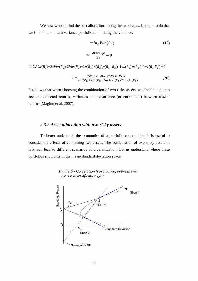
50
We now want to find the best allocation among the two assets. In order to do that
we find the minimum variance portfolio minimizing the variance:
(19)
= 0
2xVar( +2xVar( -2Var( )+2σ( σ( )ρ( , )-4xσ( σ( )Corr( , )=0
x = (20)
It follows that when choosing the combination of two risky assets, we should take into
account expected returns, variances and covariance (or correlation) between assets‘
returns (Maginn et al, 2007).
2.3.2 Asset allocation with two risky assets
To better understand the economics of a portfolio construction, it is useful to
consider the effects of combining two assets. The combination of two risky assets in
fact, can lead to different scenarios of diversification. Let us understand where these
portfolios should lie in the mean-standard deviation space.
Figure 6 - Correlation (covariance) between two
assets: diversification gain

51
1. Returns are perfectly positively correlated.
Correlation is: Corr( = 1
The standard deviation of the portfolio is: ( ) =
If we plot the mean and the standard deviation of the two assets, the straight line
between the two points is the set of portfolios available in this situation. Point 1
in the graph represents the portfolio in which x=1 and on the opposite side, point
2 represents the point where x=0.The geometric interpretation of this case is easy
to understand: there is no diversification gain at all.
2. Returns are perfectly negatively correlated.
Correlation is: Corr( = -1
The standard deviation is: σ( ) =
In this situation, with the right choice of weights on each asset, it is possible to
have a standard deviation of the portfolio equal to 0. Graphically, it corresponds
to point y in the diagram: there is a full diversification gain.
3. Returns are imperfectly correlated.
Correlation is : Corr( ∈ [-1,1]
The standard deviation of the portfolio is the square root of the variance of
Formula 18. More realistically, the correlation between assets tends to be
between the positive and the negative one. The curve of the diagram plots the
possible portfolios with correlation between 0 and 1.
Note that the weights of the portfolio do not have restrictions on the sign so a
negative x can be considered as a short sale of asset 1. The dotted line extension of the
line in Figure 6 represents short sales: through short selling it is possible to change
perfectly positive correlation into negative correlation.
The graph of the lowest possible portfolio variance that is attainable for a given
portfolio expected return is the minimum-variance frontier. Investors, however, only
care about a certain portion of the frontier, that is the portion with positive slope,
because the part with a negative slope implies lower returns for greater standard
deviation and investors would not buy this trade-off. Portfolios on the efficient frontier
are mean-variance efficient since there is not another portfolio with the same expected
return and lower standard deviation, or, equivalently, there is not another portfolio with
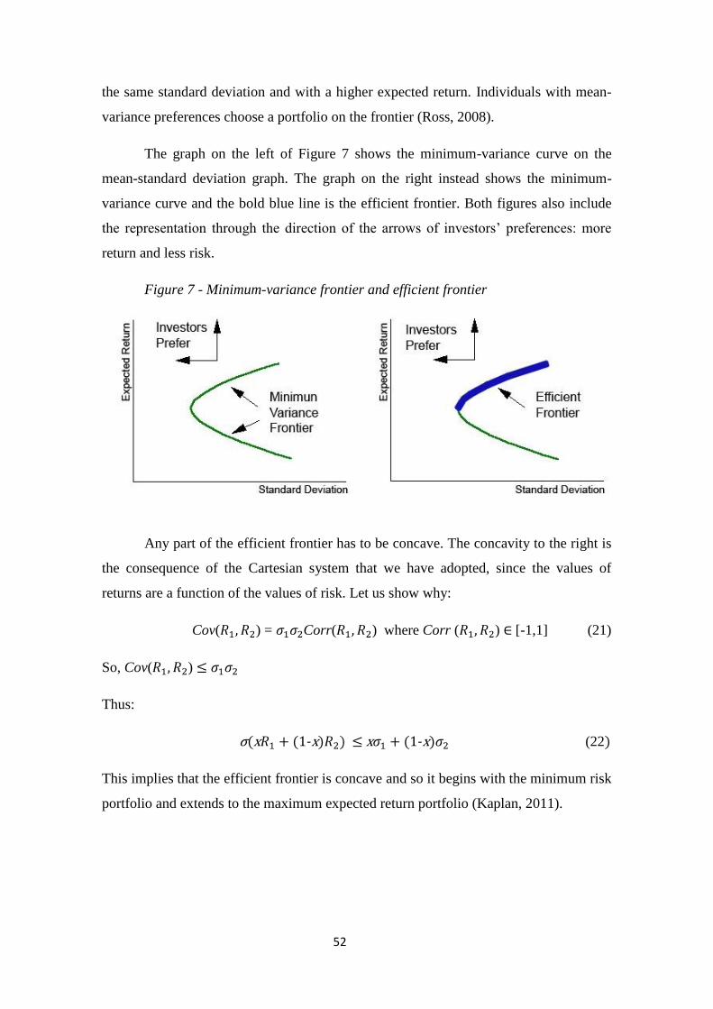
52
the same standard deviation and with a higher expected return. Individuals with mean-
variance preferences choose a portfolio on the frontier (Ross, 2008).
The graph on the left of Figure 7 shows the minimum-variance curve on the
mean-standard deviation graph. The graph on the right instead shows the minimum-
variance curve and the bold blue line is the efficient frontier. Both figures also include
the representation through the direction of the arrows of investors‘ preferences: more
return and less risk.
Figure 7 - Minimum-variance frontier and efficient frontier
Any part of the efficient frontier has to be concave. The concavity to the right is
the consequence of the Cartesian system that we have adopted, since the values of
returns are a function of the values of risk. Let us show why:
Cov( ) = Corr( ) where Corr ( ) ∈ [-1,1] (21)
So, Cov( ) ≤
Thus:
σ(x + (1-x) ≤ x + (1-x) (22)
This implies that the efficient frontier is concave and so it begins with the minimum risk
portfolio and extends to the maximum expected return portfolio (Kaplan, 2011).
53
2.3.3 Introducing a risk-free asset and the Tobin’s separation
theorem: the CML
Let us consider the scenario in which investors are allowed to borrow or lend at
the risk free rate while still investing in any single risky bundle on the efficient
frontier. For each single risky bundle, there is a new set of risk-return combination
known as the transformation line that is a straight line that goes from the risk free rate
on the expected return axis to each single risky bundle and an investor can be anywhere
on this line. The transformation line that is tangential to the efficient frontier is the
Capital Market Line (CML). The tangent point defines the single composition of risky
assets that the investor wants to hold (Sharpe, 1964).
Let us now provide a more detailed analysis about what we have just described.
We take a risk-free security like a Treasury Bill and we take a portfolio that is a
combination of a risky asset, asset 1, and a risk-free asset. The risk free asset has of
course zero risk and so it has standard deviation equal to zero, moreover, there is no
correlation with the risky asset:
(23)
Expected return of the portfolio is:
E( ) = xE( + (1-x) (24)
And the variance is:
Var( (25)
From the precedent mean and variance expressions we obtain the expected
return of the portfolio and the optimal weight, x, on the risky asset:
E( )= + x[E( ) - ] (26)
→ x = (27)
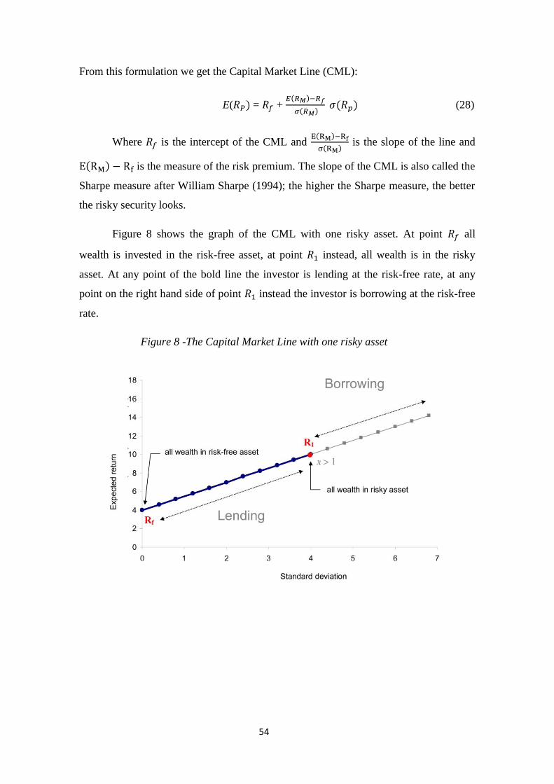
54
From this formulation we get the Capital Market Line (CML):
E( = + (28)
Where is the intercept of the CML and is the slope of the line and
is the measure of the risk premium. The slope of the CML is also called the
Sharpe measure after William Sharpe (1994); the higher the Sharpe measure, the better
the risky security looks.
Figure 8 shows the graph of the CML with one risky asset. At point all
wealth is invested in the risk-free asset, at point instead, all wealth is in the risky
asset. At any point of the bold line the investor is lending at the risk-free rate, at any
point on the right hand side of point instead the investor is borrowing at the risk-free
rate.
Figure 8 -The Capital Market Line with one risky asset
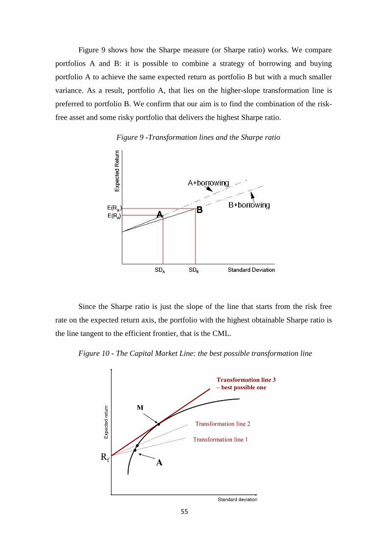
55
Figure 9 shows how the Sharpe measure (or Sharpe ratio) works. We compare
portfolios A and B: it is possible to combine a strategy of borrowing and buying
portfolio A to achieve the same expected return as portfolio B but with a much smaller
variance. As a result, portfolio A, that lies on the higher-slope transformation line is
preferred to portfolio B. We confirm that our aim is to find the combination of the risk-
free asset and some risky portfolio that delivers the highest Sharpe ratio.
Figure 9 -Transformation lines and the Sharpe ratio
Since the Sharpe ratio is just the slope of the line that starts from the risk free
rate on the expected return axis, the portfolio with the highest obtainable Sharpe ratio is
the line tangent to the efficient frontier, that is the CML.
Figure 10 - The Capital Market Line: the best possible transformation line
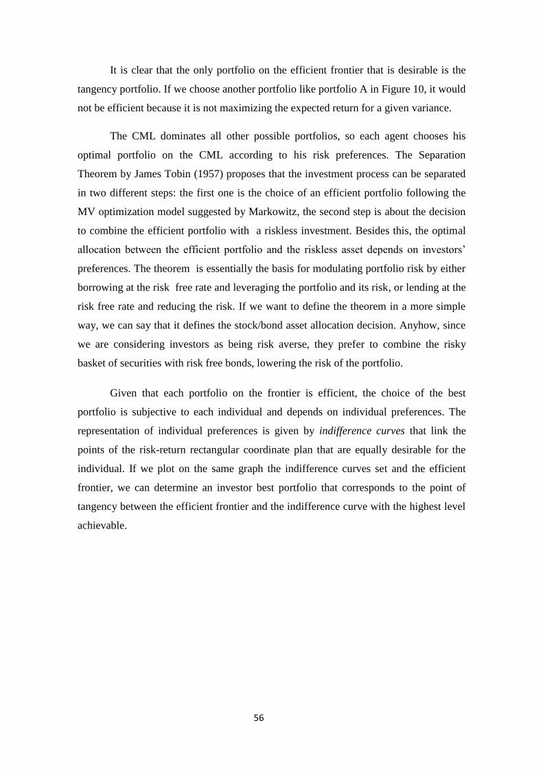
56
It is clear that the only portfolio on the efficient frontier that is desirable is the
tangency portfolio. If we choose another portfolio like portfolio A in Figure 10, it would
not be efficient because it is not maximizing the expected return for a given variance.
The CML dominates all other possible portfolios, so each agent chooses his
optimal portfolio on the CML according to his risk preferences. The Separation
Theorem by James Tobin (1957) proposes that the investment process can be separated
in two different steps: the first one is the choice of an efficient portfolio following the
MV optimization model suggested by Markowitz, the second step is about the decision
to combine the efficient portfolio with a riskless investment. Besides this, the optimal
allocation between the efficient portfolio and the riskless asset depends on investors‘
preferences. The theorem is essentially the basis for modulating portfolio risk by either
borrowing at the risk free rate and leveraging the portfolio and its risk, or lending at the
risk free rate and reducing the risk. If we want to define the theorem in a more simple
way, we can say that it defines the stock/bond asset allocation decision. Anyhow, since
we are considering investors as being risk averse, they prefer to combine the risky
basket of securities with risk free bonds, lowering the risk of the portfolio.
Given that each portfolio on the frontier is efficient, the choice of the best
portfolio is subjective to each individual and depends on individual preferences. The
representation of individual preferences is given by indifference curves that link the
points of the risk-return rectangular coordinate plan that are equally desirable for the
individual. If we plot on the same graph the indifference curves set and the efficient
frontier, we can determine an investor best portfolio that corresponds to the point of
tangency between the efficient frontier and the indifference curve with the highest level
achievable.
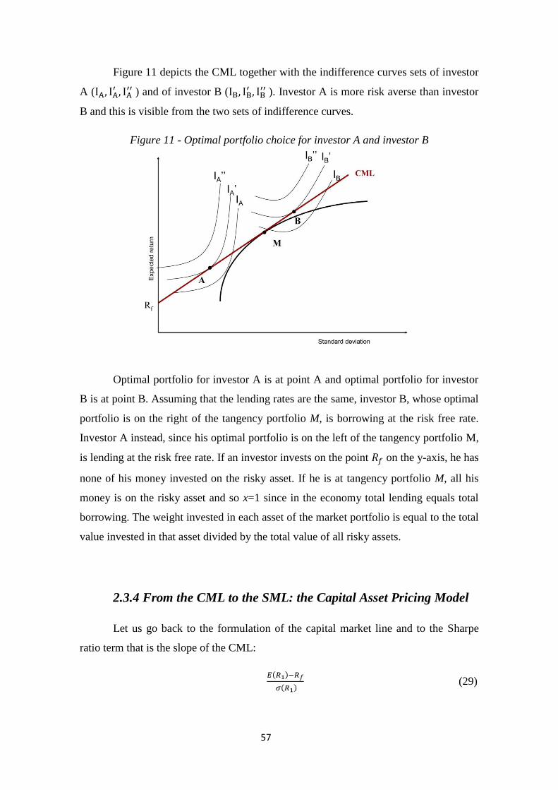
57
Figure 11 depicts the CML together with the indifference curves sets of investor
A ( ) and of investor B ( ). Investor A is more risk averse than investor
B and this is visible from the two sets of indifference curves.
Figure 11 - Optimal portfolio choice for investor A and investor B
Optimal portfolio for investor A is at point A and optimal portfolio for investor
B is at point B. Assuming that the lending rates are the same, investor B, whose optimal
portfolio is on the right of the tangency portfolio M, is borrowing at the risk free rate.
Investor A instead, since his optimal portfolio is on the left of the tangency portfolio M,
is lending at the risk free rate. If an investor invests on the point on the y-axis, he has
none of his money invested on the risky asset. If he is at tangency portfolio M, all his
money is on the risky asset and so x=1 since in the economy total lending equals total
borrowing. The weight invested in each asset of the market portfolio is equal to the total
value invested in that asset divided by the total value of all risky assets.
2.3.4 From the CML to the SML: the Capital Asset Pricing Model
Let us go back to the formulation of the capital market line and to the Sharpe
ratio term that is the slope of the CML:
(29)
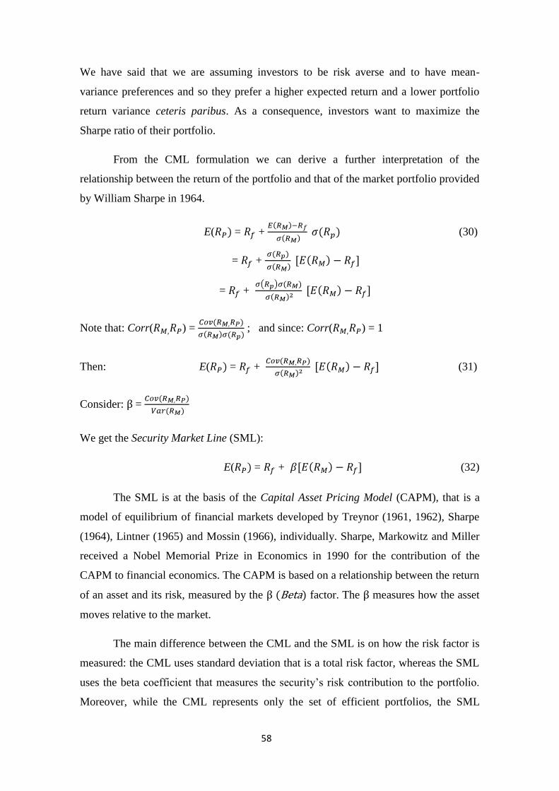
58
We have said that we are assuming investors to be risk averse and to have mean-
variance preferences and so they prefer a higher expected return and a lower portfolio
return variance ceteris paribus. As a consequence, investors want to maximize the
Sharpe ratio of their portfolio.
From the CML formulation we can derive a further interpretation of the
relationship between the return of the portfolio and that of the market portfolio provided
by William Sharpe in 1964.
E( = + (30)
= +
= +
Note that: Corr( ) = ; and since: Corr( ) = 1
Then: E( = + (31)
Consider: β =
We get the Security Market Line (SML):
E( = + (32)
The SML is at the basis of the Capital Asset Pricing Model (CAPM), that is a
model of equilibrium of financial markets developed by Treynor (1961, 1962), Sharpe
(1964), Lintner (1965) and Mossin (1966), individually. Sharpe, Markowitz and Miller
received a Nobel Memorial Prize in Economics in 1990 for the contribution of the
CAPM to financial economics. The CAPM is based on a relationship between the return
of an asset and its risk, measured by the β (Beta) factor. The β measures how the asset
moves relative to the market.
The main difference between the CML and the SML is on how the risk factor is
measured: the CML uses standard deviation that is a total risk factor, whereas the SML
uses the beta coefficient that measures the security‘s risk contribution to the portfolio.
Moreover, while the CML represents only the set of efficient portfolios, the SML
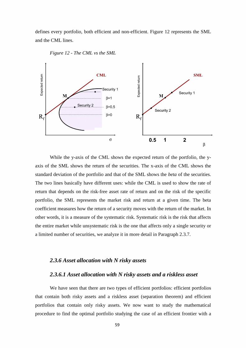
59
defines every portfolio, both efficient and non-efficient. Figure 12 represents the SML
and the CML lines.
Figure 12 - The CML vs the SML
While the y-axis of the CML shows the expected return of the portfolio, the y-
axis of the SML shows the return of the securities. The x-axis of the CML shows the
standard deviation of the portfolio and that of the SML shows the beta of the securities.
The two lines basically have different uses: while the CML is used to show the rate of
return that depends on the risk-free asset rate of return and on the risk of the specific
portfolio, the SML represents the market risk and return at a given time. The beta
coefficient measures how the return of a security moves with the return of the market. In
other words, it is a measure of the systematic risk. Systematic risk is the risk that affects
the entire market while unsystematic risk is the one that affects only a single security or
a limited number of securities, we analyze it in more detail in Paragraph 2.3.7.
2.3.6 Asset allocation with N risky assets
2.3.6.1 Asset allocation with N risky assets and a riskless asset
We have seen that there are two types of efficient portfolios: efficient portfolios
that contain both risky assets and a riskless asset (separation theorem) and efficient
portfolios that contain only risky assets. We now want to study the mathematical
procedure to find the optimal portfolio studying the case of an efficient frontier with a

60
riskless asset and N risky assets and the case of an efficient frontier with no riskless
asset.
To proceed with the analysis of the first case we need to collect several data like
expected returns on all assets, variances and covariances on all asset returns and the
riskless borrowing and lending rate, in order to construct the CML. We define:
X: the generic vector of the weights of the portfolio (proportion of wealth invested
in each asset);
R: the vector of returns of all the assets traded in the market;
: the return of each asset in the market
Ω: the variance-covariance matrix
1: a vector with all 1 such that =
Let us illustrate the matrices:
X = R = Ω =
We want to find the optimal portfolio given by the combination of the risky
assets with the risk-free asset, that is the tangency portfolio. We proceed maximizing
the slope of the tangent line subject to the budget constraint, e.g. the sum of the
portfolio weights is one:
(33)
We set:
(34)
So:
= (35)
= (R- ) + [ (R- )](- )2ΩX = 0
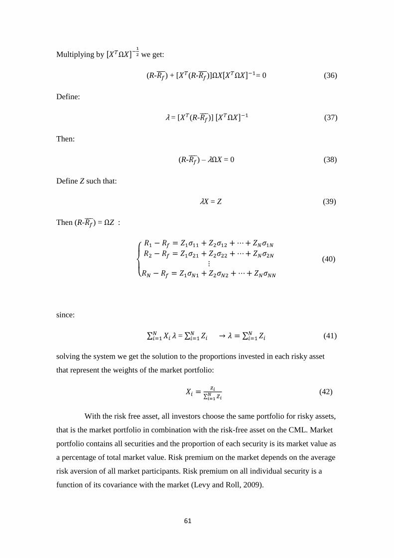
61
Multiplying by we get:
(R- ) + [ (R- )]ΩX = 0 (36)
Define:
λ = [ (R- )] (37)
Then:
(R- ) – λΩX = 0 (38)
Define Z such that:
λX = Z (39)
Then (R- ) = ΩZ :
(40)
since:
= (41)
solving the system we get the solution to the proportions invested in each risky asset
that represent the weights of the market portfolio:
(42)
With the risk free asset, all investors choose the same portfolio for risky assets,
that is the market portfolio in combination with the risk-free asset on the CML. Market
portfolio contains all securities and the proportion of each security is its market value as
a percentage of total market value. Risk premium on the market depends on the average
risk aversion of all market participants. Risk premium on all individual security is a
function of its covariance with the market (Levy and Roll, 2009).

62
2.3.6.2 Efficient frontier with N risky assets and no riskless asset
Let us suppose there is no riskless asset. In order to find the optimal portfolio
we minimize portfolio variance subject to two constraints:
1. minimization occurs for a given level of expected return;
2. the budget constraint: the sum of the portfolio weights is one.
Expected return of the portfolio is:
E( ) = X = (43)
And the variance of the portfolio is:
Var( ) = ΩX (44)
For a given level of portfolio expected return E( ) we want to minimize the variance.
The quadratic programming problem is:
(45)
u.c.
The Lagrangian is:
£ = (46)
The terms λ and γ are the Lagrangian multipliers. We solve:
(47)
We get:
X = Equation 4 from Equation 1

63
And:
(48)
We define some constants:
A = (49)
B =
C =
D = BC -
Solving the system for and we get:
(50)
It follows: X = g+hE( )
with g = (51)
h = (52)
Portfolio g represents the optimal weights of a portfolio with E( ) = 0
X = g+h represents the optimal weights of a portfolio with E( ) = 1 (Levy and Roll,
2009).
Finally, the formulation of the efficient frontier in this scenario is given by Formula 53:
V( ) = (53)
This is a second order equation in E( ) that is indentified as an hyperbole in a
Cartesian plan with V( ) on the x-axis and E( ) on the y-axis.
64
2.3.7 Systematic and unsystematic risk
The risk of an investment is the amount an asset deviates from its expected
value. Total risk, however depends on two types of investment risk: systematic and
unsystematic (or idiosyncratic) risk.
Total risk = Systematic risk + Unsystematic risk
Systematic risk is associated to the risk inherent to the entire market, it is not
linked to a particular stock or industry but it depends on factors associated to the market
like business cycles, geopolitics, natural disasters and market-wide economic events like
recessions, wars and interest rates. This type of risk is unpredictable and impossible to
completely avoid so there is not a particular method to handle it. This is why it is also
called non-diversifiable risk or market risk. A good way to measure the systematic risk
(volatility) of a portfolio with respect to the whole market, is the Beta coefficient ( ).
Beta can be interpreted as the tendency of a security to answer to the swings of the
market. A β equal to one indicates that the price of the security moves with the market,
in fact since all risk is measured relative to the market portfolio, the β of the market
portfolio must be one. A lower than one means that the security is less volatile than
the market so the asset has less risk relative to the market portfolio and a β greater than
one indicates that the price of the security is more volatile than the market and it has
more risk relative to the market portfolio.
Unsystematic risk is defined as firm-specific risk since it is related to a specific
company or a specific industry sector. Examples of unsystematic risk are events like the
management change of a company, competition, strikes, weather conditions and labor
problems. Unsystematic risk can be reduced through diversification. Diversification is
obtained through the creation of a portfolio that invests in various assets that are not
affected by market events in the same way. A well diversified portfolio invests in stocks
of different companies and industries and in different types of securities. The
optimization strategy that we have seen in the previous paragraphs are all based on the
concept of diversification when investing and on the idea that asset prices change in
different, sometimes opposite, ways. The term ―diversification‖ was born with
Markowitz in 1952 while Gibson (1990), Perold (2004) and others introduced the term
diversification effect to refer to the relationship between correlation among assets and
portfolio risk. Diversification effect is the phenomenon of reduction of the portfolio

65
risk that is created by correlations (usually imperfect) between assets. The importance
of diversification stays in the fact that it can help investors to manage and reduce their
investment risk, without compromising the rate of return since correlations are
independent of the rate of return. Correlation coefficients are widely used by financial
analysts to measure the diversification effect in portfolio management. However, total
riskiness of a portfolio cannot be totally eliminated because of systematic risk.
Let us see the effect that diversification has on variance in an equally-weighted
portfolio with weight on asset i and . The general formula for
calculating the portfolio return variance is given by the sum of each term variance plus
all pair-wise covariances:
= + (54)
The portfolio variance then becomes:
= + (N-1) (55)
And we get the asymptotic formula:
(56)
If N is large, (1/N) is small and (N-1)/N) is close to 1. Hence ≈ .
This means that in an equally-weighted portfolio, the portfolio variance tends to
the average of covariances between securities as the number of securities becomes large
and portfolio risk is a sort of ―covariance risk‖.
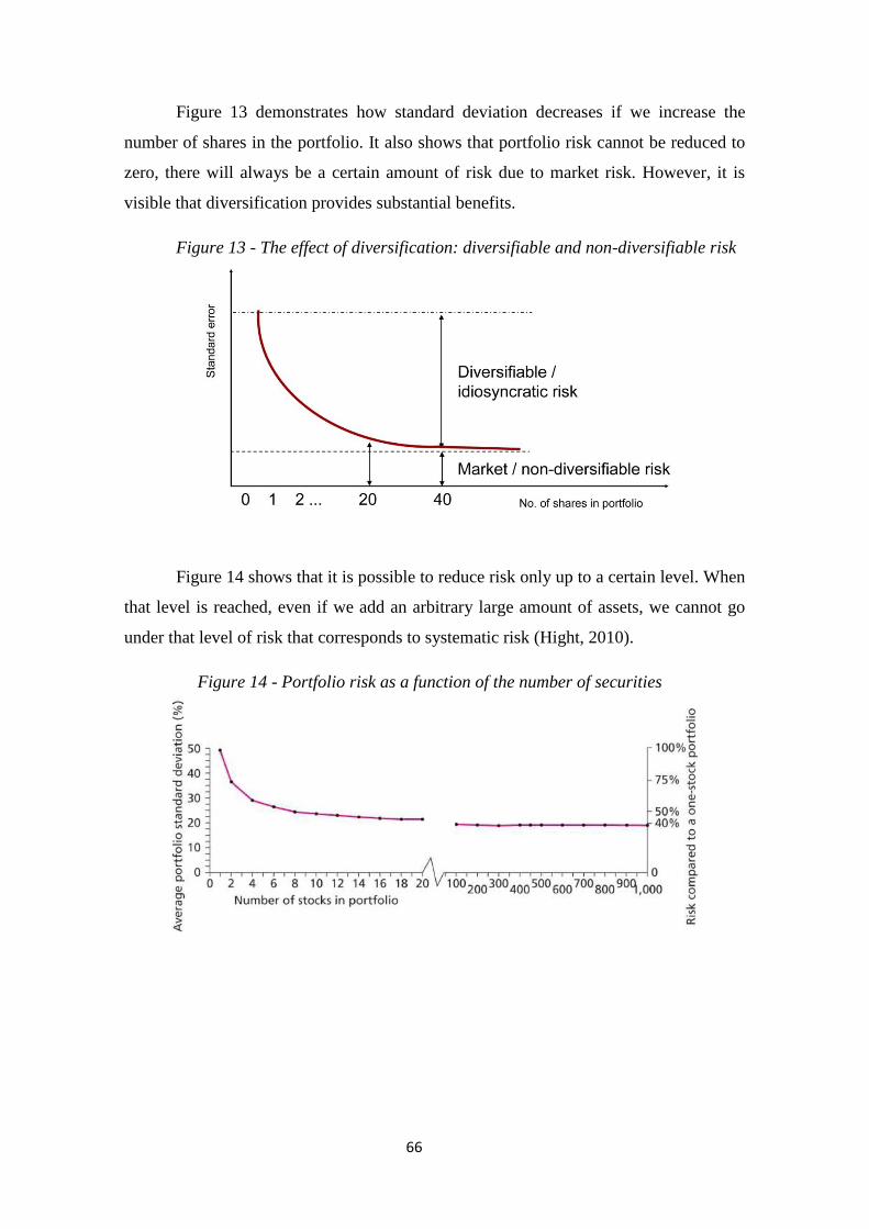
66
Figure 13 demonstrates how standard deviation decreases if we increase the
number of shares in the portfolio. It also shows that portfolio risk cannot be reduced to
zero, there will always be a certain amount of risk due to market risk. However, it is
visible that diversification provides substantial benefits.
Figure 13 - The effect of diversification: diversifiable and non-diversifiable risk
Figure 14 shows that it is possible to reduce risk only up to a certain level. When
that level is reached, even if we add an arbitrary large amount of assets, we cannot go
under that level of risk that corresponds to systematic risk (Hight, 2010).
Figure 14 - Portfolio risk as a function of the number of securities
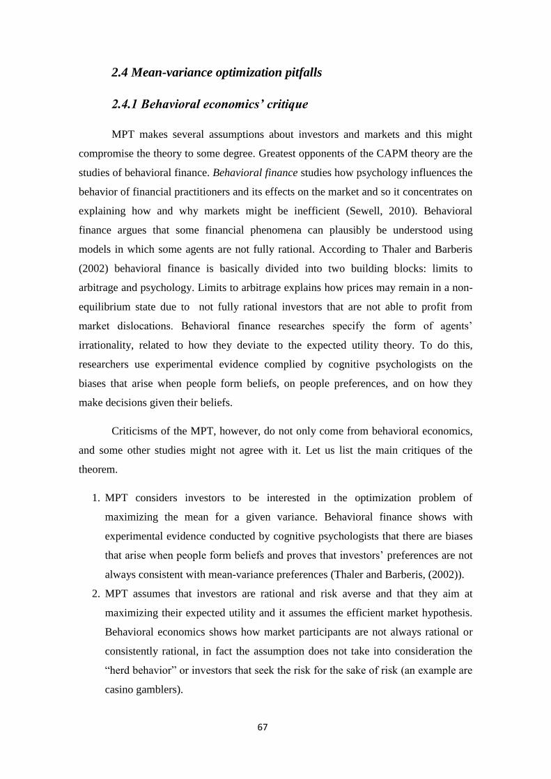
67
2.4 Mean-variance optimization pitfalls
2.4.1 Behavioral economics’ critique
MPT makes several assumptions about investors and markets and this might
compromise the theory to some degree. Greatest opponents of the CAPM theory are the
studies of behavioral finance. Behavioral finance studies how psychology influences the
behavior of financial practitioners and its effects on the market and so it concentrates on
explaining how and why markets might be inefficient (Sewell, 2010). Behavioral
finance argues that some financial phenomena can plausibly be understood using
models in which some agents are not fully rational. According to Thaler and Barberis
(2002) behavioral finance is basically divided into two building blocks: limits to
arbitrage and psychology. Limits to arbitrage explains how prices may remain in a non-
equilibrium state due to not fully rational investors that are not able to profit from
market dislocations. Behavioral finance researches specify the form of agents‘
irrationality, related to how they deviate to the expected utility theory. To do this,
researchers use experimental evidence complied by cognitive psychologists on the
biases that arise when people form beliefs, on people preferences, and on how they
make decisions given their beliefs.
Criticisms of the MPT, however, do not only come from behavioral economics,
and some other studies might not agree with it. Let us list the main critiques of the
theorem.
1. MPT considers investors to be interested in the optimization problem of
maximizing the mean for a given variance. Behavioral finance shows with
experimental evidence conducted by cognitive psychologists that there are biases
that arise when people form beliefs and proves that investors‘ preferences are not
always consistent with mean-variance preferences (Thaler and Barberis, (2002)).
2. MPT assumes that investors are rational and risk averse and that they aim at
maximizing their expected utility and it assumes the efficient market hypothesis.
Behavioral economics shows how market participants are not always rational or
consistently rational, in fact the assumption does not take into consideration the
―herd behavior‖ or investors that seek the risk for the sake of risk (an example are
casino gamblers).
68
3. The assumption that asset returns are jointly normally distributed random
variables is highly criticized since reality shows that returns in the equity markets
are not normally distributed. A study of Mandelbrot and Hudson (2004) proves
that market returns have a volatility that goes from 3 to 6 standard deviations from
the mean with more frequency than in a normal distribution assumption. MPT is
also proven by the assumption that any return distribution is jointly elliptical,
however, studies of Chamberlain (1983) and Owen and Rabinovitch (1983) prove
that all jointly elliptical distributions are symmetrical but asset returns empirically
are not.
4. MPT assumes investors to have access to the same information. Anyhow, real
markets show market asymmetry and insider trading since some actors in the
financial market generally know more than others.
5. Behavioral economics criticizes the psychological assumptions made over
investors whose probabilities of beliefs match the distribution of returns. Daniel,
Hirshleifer and Subrahmanyam (2001) provide an alternative to the CAPM model
based on behavioral economics. The model takes into account investor‘s
overconfidence about the precision of private information and investor
misevaluation: investors use information incorrectly when they form portfolios
and this leads to market under-reactions or overreactions causing equilibrium
prices to be mispriced.
6. According to MPT, correlations between assets are constant and fix forever.
However, this can be proved to be wrong. Correlation is linked to the systemic
relationship between assets. But if we consider for example financial crisis, all
assets become positively correlated because they all move down together. This
shows that when investors need risk protection, the MPT breaks.
7. Another pitfall of the MPT is that it considers no taxes and transaction costs. But
in reality, all financial products are subject to taxes and transaction costs and the
fact that they are not taken into account might compromise the composition of the
optimum portfolio.
8. Investors are price-takers and their actions do not influence prices. This
assumption is subject to critiques if we consider that in reality, sufficiently large
sales or purchases of a specific asset shift the market price for that asset. But the
market price also shifts for other assets, because of the cross elasticity of demand.
69
It follows that, if the market is changing while investors are choosing the optimal
portfolio, investors do not make an optimal choice.
9. MPT assumes that any investor can lend and borrow an unlimited amount at the
risk free rate: in reality, only the government can borrow at the risk free rate. No
other investor can borrow money at this rate unless there are special concessions.
Moreover, short selling is illegal or severely restricted in many countries.
10. The fact that securities can be divided into parcels of any size is not strictly
true since reality shows that fractional shares cannot be bought or sold and some
assets have minimum order sizes.
11. It is not always true, as MPT states, that risk and volatility are known in
advance and that they are constant: markets tend to misprice risk and the volatility
might change rapidly. An example are financial bubbles and crisis.
2.4.2 The Single Index Model
Mean-variance needs a large amount of data (expected returns, volatility,
correlations) and estimated portfolio weights are sensitive to estimation errors and so
small changes in mean returns have large effects on the efficient portfolio weights
(Jorion, 1991). Moreover, there is uncertainty about how long past time is necessary for
estimates, since volatility and correlations change over time. Also, it is a single period
model and does not consider rebalancing, it also does not consider transaction costs
such as bid-ask spread, price pressure (market impact) and brokerage. All these leads to
the definition of a non efficient portfolio and compromises the optimal choice of
investment.
Let us concentrate on the very large number of input values required to apply the
MV approach:
N expected returns for N assets;
N variances for N assets;
N (N-1)/2 correlations for N assets (we divide by 2 since = ).
To sum up we need 2N + N(N-1)/2 estimates for the mean variance analysis. This
means that for a portfolio with 50 assets we need 1.325 estimations.
70
The single-index (SI) model developed by Sharpe (1964) is a good way to solve
this problem. The model defines that the rate of return on a broad index of securities is a
valid proxy for the common macroeconomic factor and so a market index is a common
factor describing stock returns. The single-index model uses a similar equation to the
MV model but it uses a proxy for the common or systematic factor. The excess return
of stock i is divided into two parts: a macro or systematic component and a micro or
firm-specific component:
(57)
(58)
where is the market excess return and is the residual. The overall risk
of each security has two components:
a market-related part, where measures the sensitivity of a stock to market
movements;
a non-market-related part, .
Therefore, the expected return can be written as:
(59)
since it is assumed that E( ) = 0.
As a consequence, also the overall risk of each security has two components:
market or systematic risk and firm-specific risk. Hence, the variance of return on asset i
is:
+ Var( ) (60)
And it is obtained from taking the variance operator on both sides of the single index
model.
Since securities are related only in their response to the market, they covary
together only because of their relationship to the market index:
Cov( = Cov = (61)
71
Note that E[ and E[ . Using this model the number of inputs required is
substantially reduced. In fact we need:
N estimates of the extra-market expected excess returns ;
N estimates of the sensitivity coefficients ;
N estimates of the firm-specific variances ;
1 estimate for the variance of the common factor ;
1 estimate for the market risk premium E( ).
For a total of (3N+2) estimates. So in our example of a 50-security portfolio, we need
152 estimates instead of 1.325 estimates required if we apply the mean-variance
procedure.
Regression analysis is often used to estimate an index model. In fact, we can
summarize the result in a scatter diagram drawing the best fitting line through the
scatter. Each point of the diagram is defined by a pair of excess return: the y-axis
indicates the excess return of individual security in the portfolio and the x-axis indicates
the excess market return. The best line is a regression line defined through the least
squares approach: the overall solution minimizes the prediction error, e.g. the deviation
of the data points from the prediction data points. Deviations are squared in order not to
have positive and negative deviations to cancel each other out. Generally, in a single
variable regression equation, the dependent variable plots around an intercept α and a
slope β, the deviations (residuals, ε) from the line are assumed to be mutually
uncorrelated as well as uncorrelated with the independent variable. These assumptions
of regression models perfectly fit the single index model. Each residual is given by the
difference between the actual stock return and the return predicted from the regression
equation. The estimated regression equation of the single-index model is usually defined
as the security characteristics line (SCL).
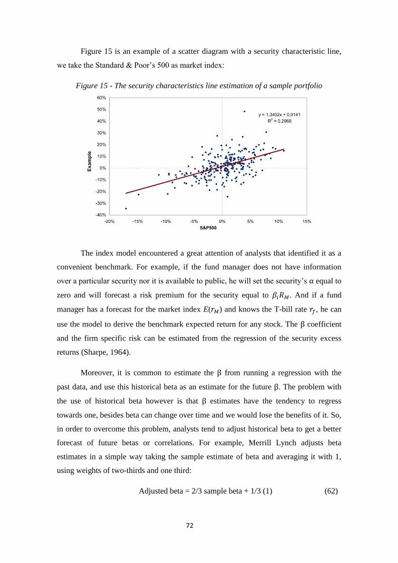
72
Figure 15 is an example of a scatter diagram with a security characteristic line,
we take the Standard & Poor‘s 500 as market index:
Figure 15 - The security characteristics line estimation of a sample portfolio
The index model encountered a great attention of analysts that identified it as a
convenient benchmark. For example, if the fund manager does not have information
over a particular security nor it is available to public, he will set the security‘s α equal to
zero and will forecast a risk premium for the security equal to . And if a fund
manager has a forecast for the market index E( ) and knows the T-bill rate , he can
use the model to derive the benchmark expected return for any stock. The β coefficient
and the firm specific risk can be estimated from the regression of the security excess
returns (Sharpe, 1964).
Moreover, it is common to estimate the β from running a regression with the
past data, and use this historical beta as an estimate for the future β. The problem with
the use of historical beta however is that β estimates have the tendency to regress
towards one, besides beta can change over time and we would lose the benefits of it. So,
in order to overcome this problem, analysts tend to adjust historical beta to get a better
forecast of future betas or correlations. For example, Merrill Lynch adjusts beta
estimates in a simple way taking the sample estimate of beta and averaging it with 1,
using weights of two-thirds and one third:
Adjusted beta = 2/3 sample beta + 1/3 (1) (62)
73
2.4.3 The Black-Litterman model
Institutional investors using the modern portfolio theory experienced the pitfalls
of the model and elaborated several solutions. It is the case of Black and Litterman
(1992) that created a development of the mathematical model for portfolio allocation for
the investment banking firm Goldman Sachs. The model tries to solve the problem of
non-realistic final allocations caused by the high number of inputs required in the MV
approach: there may be frequent estimation errors that lead to the determination of non-
efficient portfolios.
The Black-Litterman model solves the problem of non-efficient and non-realistic
portfolios introducing a subjective component to the mathematical optimization model
creating portfolios that are more intuitive and less unrealistic. This is done through the
introduction of the ―views‖ of the money managers about the asset returns. More
specifically, the model assumes that the initial expected return is proportional to the
market values of the available assets but it is later modified according to the specific
opinion about the asset returns. Every institutional investor should state his assumptions
about expected returns and the degree of confidence in the assumptions and see how
they differ from those of the market. The level of confidence equilibrates the impact on
the final asset allocation with respect to the prevision model: as the confidence
increases, the distance to the optimal asset allocation of the prevision model increases.
This methodology is very flexible because the money manager does not
necessarily have to express his opinion on all the activities stock classes of the
provisional model and the final allocation does not necessarily have to be distant from
the provisional model. Black and Litterman in fact start from the MV equilibrium
expected returns as the necessary input for the formulation of the investment decision
(Black and Litterman, 1992).
2.4.4 Roll’s critique
Roll (1977) suggests that the CAPM cannot be subject to an empirical proof. In
fact, every test conducted on the CAPM needs to consider the hypothesis that the
market portfolio belongs to the efficient frontier. However, the market portfolio
should contain all the financial activities available in the market, this means that it does
74
not contain only stocks and bonds, but also other entities that are not easily identifiable
like human capital, real estate and artworks. Since it is hard to include everything that
has a marketable value, it follows that the market portfolio is just a proxy of the real
market portfolio and does not provide a legitimate conclusion on the mean-variance
efficiency.
Roll considerations also include that: the only testable hypothesis of the asset
pricing model of Black is that the market portfolio is mean-variance efficient and that
all the implications of the model, the best known of which is the linearity relation
between expected return and beta, are not independently testable. Also, he says that
using proxies might be mean variance efficient even when the true market portfolio is
not:
―This is real danger since every sample will display efficient portfolios that
satisfy perfectly all of the theory‘s implications. For example, suppose there exist 1000
assets but only 500 are used in the sample. For the sample, there will exist well
diversified portfolios of the 500 assets that seem to be reasonable proxies for the market
and for which observed returns are exactly linearly related cross-sectionally to observe
betas. On the other hand, the chosen proxy may turn out to be inefficient; but obviously
this alone implies nothing about the true market portfolio‘s efficiency‖ (Roll, 1977).
Roll‘s critique makes us remember that the effort to know the market as a hole is
only an attempt. Even if the Roll‘s critique has a valid theoretical fundamental,
however, the CAPM is still widely used and its supporters consider market indices as a
proxy for the overall market. Also financial websites like Yahoo! Finance, Bloomberg
and Morningstar frequently estimate the beta of the firms, taking into account the
weaknesses associated with any empirical test.
2.5 The benchmark and the portfolio management strategy
As we said in Chapter 1, the asset management industry has recently widely
developed and investors tend to delegate the management of their savings to
institutional investors. In this scenario it grows the importance of performance
evaluation through which it is possible to evaluate the portfolio management both from
the side of the return from the investment and of the riskiness of the investment. For the

75
purpose of evaluation, it is necessary to choose the right benchmark to be taken as a
reference point to estimate the performance of the fund considering the management
style in that specific period.
The benchmark is an index or a mix of indices that synthesizes the movement of
the markets in which a fund invests, and it is the parameter that allows a comparison of
performance for a mutual fund. The introduction of the benchmark in Italy took place in
1998 with its imposition by the Consob19
as an objective reference parameter. The
benchmark is a very useful instruments and it has several advantages:
it helps in the identification of the investment: it explicitly defines the risk ex-ante of
an asset class and of the type of investment, assisting investors in the choice of a
coherent solution for their objectives;
it is useful for the evaluation of the results of the fund: it allows to measure on a
specific time frame the quality of the management;
it is representative of a market: every index that belongs to the benchmark is
representative of that specific market;
it has a transparent construction: every index is composed and calculated with clear
and simple rules accessible to investors.
When comparing the returns of the benchmark with those of the fund, it is
important to keep in mind that the benchmark is a sort of virtual fund, since it would be
impossible for a real fund to invest in all the titles of the market, also because they tend
to have several constraints of accessibility to some market segments. Moreover, the
benchmark is not subject to the costs that a real portfolio has, like management costs,
distribution costs, negotiation costs and administrative costs. Furthermore, the time
frame of analysis is fundamental for the comparison, if the comparison is made on a
time frame that is not adequate to the type of investment, it loses the significance. The
benchmark of a fund must always be indicated, and in the case in which it is impossible
to identify it, the reasons of this impossibility must be indicated. Moreover, it is
necessary to indicate which is the relationship between the benchmark and the objective
of the fund. The benchmark can also be identified as a reference for the quality of the
investment instrument. In Italy a benchmark is correct only if it respects the regulation
of the Consob.
19
Consob Regulation n. 11522 of the 1st of July 1998, Art. 50, 2.
76
As far as the portfolio style is concerned, it basically defines the way in which a
fund is managed. Firstly, we analyze the difference between active and passive
management.
1. Active management. When a fund is actively managed, the portfolio composition of
the fund is voluntarily different from that of the benchmark. The objective is to have
a higher return than that of the market index chosen as benchmark by the fund
manager. The choice of the benchmark is the consequence of an accurate selection of
stocks (―stock picking‖), of the anticipation of the movements of value of the stocks
(―market timing‖) and of the allocation on different markets and activities (―asset
allocation‖). The logic behind this is that of exposing the portfolio to a higher risk
than that of the benchmark: if the strategy is successful the higher risk will generate a
higher return from the benchmark, otherwise the return will be lower.
2. Passive management. When a fund is passively managed, the composition of its
portfolio is chosen on the basis of a pre-established objective like the replication of
an index (benchmark) and the number and volume of transactions is limited. A
passively managed fund usually has lower commission costs since it needs a lower
effort to be managed.
Investment performance attribution studies the causes of the active return of a
portfolio through the decomposition of the active return into single components
identifiable in the active management process. There are three main activities that
contribute to the generation of active return:
1. Strategic asset allocation is the activity that identifies the level of specialization or
diversification of the portfolio, the level of risk and liquidity, the areas of investment
between stocks, bonds and liquidities, geographic areas and business sectors, and the
correlation between the different financial instruments on the basis of a time period.
Through the combination of the elementary asset classes it is possible to obtain an
infinite number of combinations and create an asset class composite. Strategic asset
allocation is all about targeting allocation and then periodically rebalancing with the
change of the goals and needs of the client.
2. Tactical asset allocation or market timing sets a range of percentages (that is the
maximum and the minimum acceptable percentage) in each asset class. Investors can
move through this percentage, for example increase up to the upper threshold the
percentage of stocks held in the portfolio if the markets are doing well, and diminish
77
it up to the minimum threshold when the economic outlook is bleak. Market timing is
the act of attempting to predict the future direction of the market through the use of
technical indicators and economic data but also the practice of switching among
mutual fund asset classes in an attempt to profit from the changes of the market
outlook.
3. Stock picking or security selection is the activity through which an analyst uses a
systematic form of analysis to evaluate whether a particular stock is a good
investment or not and to decide whether it should be added to his portfolio
(Luenberger, 2006).
There are two management strategies that contribute to generate the active
component: the top-down and the bottom-up approach. The top-down approach is
conducted through a macro analysis that allows to define a portfolio. The objective of
the analysis is to provide the indications linked to the evolutions of the market and
sector and explains the risk about them. All these analysis are correlated and allow to
define the strategic choices of investment. The approach is called top-down since it
starts from the analysis of the macro economic variables that might influence the
markets in a predetermined period. The bottom-up approach instead starts from the
analysis of a single firm to find the opportunities of profit. In general, the analysts that
follow this approach are specialized in a single sector, geographic area or State. When
analyzing a firm they start from the study of the balance sheet, the strategic positioning
of the firm, and the market in which it works. The analysis allows them to select the
firms that provide higher expected profits.
A debate over actively and passively managed funds has developed in the last
years. Of course each investor worries about the ability of money managers to create
extra performance, asset management in fact is a valuable option only if the
management of the fund is able to use the information in his possession to make
previsions of the market movements and to generate a portfolio with greater returns than
the benchmark. But this is not confirmed by several studies and researches, first of all
the market efficiency hypothesis by Fama (1965) states that any attempt to look for
information to find the mispriced assets is vain: when markets are efficient all the
stocks in the market have the right price since they immediately reflect the available
information to all market participants and consequently no one can beat the market.
Jensen (1968) evaluates the performance of mutual funds and finds no evidence of
78
managers‘ skills. Some other empirical researches confirm the superiority of passive
management with respect to active management due to the high transaction costs. An
important study by Brinson, Beebower and Singer (1991) conducted on 91 pension
funds in the United States in the period 1974-1983 demonstrates that over 90% of the
variability of returns in a typical mutual fund over time is a direct consequence of the
long-term strategic asset allocation. Later, Ibbotson and Kaplan (2000) conducted a
study over a sample of 94 balanced funds in the US over the period 1988-1998 and over
a sample of 58 pension funds in 1993-1997. The aim of the research was to determine
how much of the variation in returns among different portfolios is explained by strategic
asset allocation differences through the use of cross-sectional analysis. The result of the
study showed that 35% of the variation of returns across portfolios is explained by
strategic asset allocation and the remaining 65% is explained by other factors like
market timing, style within asset classes, fees and manager selection. Ippolito (1989)
demonstrates the ability of active funds to beat the market but not if net of fees and
expenses. Similar results are obtained by Cesari and Panetta (2002) with a study over
Italian equity funds that finds no evidence of superior forecasting skills among Italian
fund managers. The study concentrates on the possibility that money managers choose
non-efficient benchmarks to compare their portfolios and that the phenomenon of
―survivorship bias‖ (e.g. the tendency to exclude failing companies from the studies of
performance because they no longer exist) should be considered because it causes
results to skew higher because only successful companies are taken into consideration.
They also consider the fact that there is not a persistency of the results of mutual funds:
the identification of the asset management company that beats the market is not useful
since money managers tend to shift from one company to another.
2.6 Performance and risk measurement
2.6.1 Introducing performance and risk measurement
Since the market of mutual funds has continuously grown and the number of
professionally managed funds has increased, the need for clear and accurate portfolio
performance analysis has widened. Investors want to have information to choose where
to invest, they want to know whether fund managers succeeded in reaching the
objectives and getting returns sufficiently higher to reward the risk taken and they want
79
to understand whether the results of the portfolio are due to luck or to the real skills of
the fund manager. Moreover, performance analysis generates information useful for
money managers to alter decisions made about the portfolio‘s design, since portfolio
management is a dynamic process.
When making an investment it is important to keep in mind that returns mean
nothing unless put side by side with the risk undertaken. Let us repeat a concept: total
returns on an asset are the sum of the risk free return , that is the return from the time
value of money, the beta return, which is the reward from additional volatility of the
asset, also called risk premium, and the alpha return, that is the superior performance
attributable to the asset manager security‘s selection skill. While the risk free rate brings
no volatility, the beta and alpha components carries volatility. The risk-adjusted
performance (RAP) measures allow to analyze the results of funds or stocks taking into
consideration at the same time the returns and the risk. The main feature of these
measures is that they give a measurement of the return adjusted to the level of risk taken
to obtain that level of return. Thanks to these measurements it is possible to compare the
different funds or stocks in a simple way since the necessary information is summarized
by this measure. The fund with the higher RAP is the best, since it has the best position
in the risk-return framework. Absolute risk-adjusted performance measures evaluate
funds‘ risk-adjusted returns, without any reference to a benchmark, in the next
paragraphs we are going to describe the Sharpe ratio, the Treynor ratio and the measures
based on the VaR. Relative risk-adjusted performance measures instead evaluate returns
in reference to a benchmark, we are going to describe the M2 measure, Jensen‘s alpha
and the information ratio.
2.6.2 The Sharpe index
The Sharpe index (also known as Sharpe measure or Sharpe ratio) is a reward-to
variability measure that evaluates the performance of an investment adjusted for its risk.
The ratio measures the excess return (or risk premium) per unit of deviation in an
investment asset. It is a very simple measure to define how well the return of an asset
compensates the investor for the risk he takes and it is a widely used measurement. If
we are comparing two assets with the same risk, the one with a higher Sharpe ratio
80
provides a better return (or equivalently if they have the same return but one has lower
risk). The Sharpe ratio is the slope of the CML and its formula is defined as:
= (63)
The main pitfall of the measurement is that returns have to be normally
distributed but reality proves that not all asset returns are normally distributed.
Abnormalities in the distribution like kurtosis, fatter tails, high peaks and skewness can
make the ratio not to have the same effectiveness since they have effects on standard
deviation (Sharpe, 1994).
2.6.3 The Treynor ratio
The Treynor ratio (also called Treynor measure) is a reward-to-volatility
measure, named after Jack L. Treynor. It measures returns earned in excess of what
could be earned in a riskless investment measuring the relationship between the return
on the portfolio above the risk-free rate and its systematic risk. It differs from the
Sharpe ratio for the fact that, instead of taking into account total risk, it only considers
systematic risk. The formula of the Treynor ratio of a portfolio is similar to that of the
Sharpe ratio, with the difference that the Treynor ratio uses beta as the measurement of
volatility:
= (64)
Like the Sharpe ratio, it allows to create a ranking of portfolios: the higher the
Treynor ratio, the higher the performance of the portfolio in the analysis. This
measurement derives from the CAPM and it requires the estimation of the beta of the
portfolio choosing the proper reference index, it follows that the result can depend on
the choice of that index. The Treynor ratio is a useful index if used to evaluate the
performance of a portfolio that is well diversified since it takes into account only the
systematic risk of a portfolio (Hübner, 2005),.
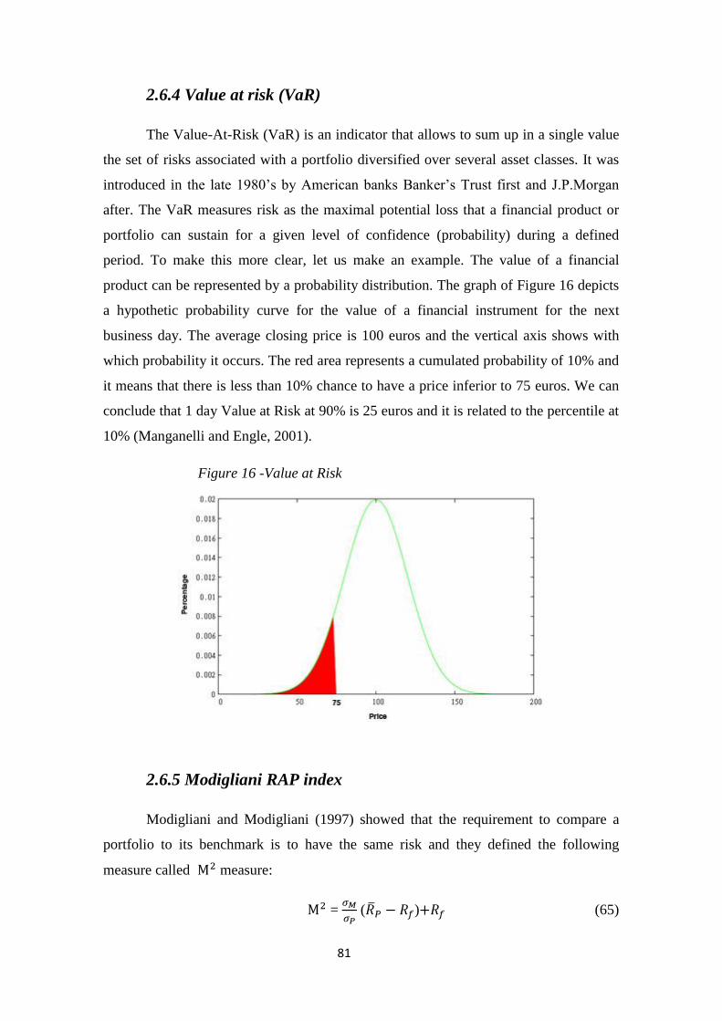
81
2.6.4 Value at risk (VaR)
The Value-At-Risk (VaR) is an indicator that allows to sum up in a single value
the set of risks associated with a portfolio diversified over several asset classes. It was
introduced in the late 1980‘s by American banks Banker‘s Trust first and J.P.Morgan
after. The VaR measures risk as the maximal potential loss that a financial product or
portfolio can sustain for a given level of confidence (probability) during a defined
period. To make this more clear, let us make an example. The value of a financial
product can be represented by a probability distribution. The graph of Figure 16 depicts
a hypothetic probability curve for the value of a financial instrument for the next
business day. The average closing price is 100 euros and the vertical axis shows with
which probability it occurs. The red area represents a cumulated probability of 10% and
it means that there is less than 10% chance to have a price inferior to 75 euros. We can
conclude that 1 day Value at Risk at 90% is 25 euros and it is related to the percentile at
10% (Manganelli and Engle, 2001).
Figure 16 -Value at Risk
2.6.5 Modigliani RAP index
Modigliani and Modigliani (1997) showed that the requirement to compare a
portfolio to its benchmark is to have the same risk and they defined the following
measure called measure:
= ( ) (65)
82
The index evaluates the risk-adjusted performance of a portfolio in relation to
the market benchmark expressed in percentage terms. The aim of the index is to identify
the return that a fund with any given risk would have achieved if it had the same risk as
the market index. This means that the index allows us to define the performance of the
fund in relation to that of the market. The most interesting funds are those with the
highest value. This measure is directly derived from the CML and it can be
expressed as the Sharpe ratio times the standard deviation of the benchmark index. The
Sharpe measure and the Modigliani measure lead to the same ranking of the funds
(Modigliani and Modigliani, 1997).
2.6.6 Jensen’s alpha
Jensen‘s alpha takes its name from the economist Michael Jensen (1968) that
first introduced it to evaluate mutual funds‘ managers. It is a measure used to determine
the abnormal return of a stock or portfolio over the theoretical return predicted by a
market model, that is most commonly the CAPM. It makes use of statistical methods to
predict the appropriate risk adjusted return of an asset and it is defined as the extra-
return of a fund with respect to the return he should have at that level of systematic risk.
It is basically the differential between the return on the portfolio in excess of the risk-
free rate and the return explained by the market model. We can define the Jensen‘s
alpha ( ) as:
= (66)
The statistical significance of alpha can be evaluated by calculating the t-statistic
of the regression, which is equal to the estimated value of the alpha divided by its
standard deviation. If the alpha values are assumed to be normally distributed, a t-
statistic greater than two indicates that the probability of having obtained the result
through luck and not through skill is strictly less than 5% and the average value of alpha
is significantly different from zero. This ratio contains a benchmark and it takes into
account only systematic risk. However, since it does not allow portfolios with different
levels of risk to be compared, it is a good measure to rank portfolios within peer groups,
that means groups that are managed in a similar manner and have comparable levels of
risk (Jensen, 1968).
83
2.6.7 Portfolio’s beta
The beta of a portfolio is used to measure the sensitivity of the returns of a fund
with respect to the market (or a benchmark) and it aims at determining whether the fund
is more risky than the market (Markowitz, 1952). Its formula is:
β = (67)
β > 1 means that asset moves in the same direction of the market but in a higher
amount;
β = 1 means that the asset moves generally in the same direction as the movement
of the benchmark and also in the same amount;
0 < β < 1 means that the asset moves in the same direction of the market but in a
lower amount than the movement of the benchmark;
β = 0 means that the movement of the asset is not correlated with the movement
of the benchmark;
β < 0 means that the asset moves in opposite direction with respect to the index.
2.6.8 Information ratio
The information ratio is defined by the residual return of the portfolio compared
to its residual risk. The residual return of a portfolio corresponds to the share of the
return that is not explained by the benchmark and results from the choice made by
managers that choose the securities that they think will beat the benchmark. The
residual risk instead is the measure of residual return variations and it is defined by the
standard deviation of the difference in return between the portfolio and its benchmark. If
the value is low, the risk of the portfolio is close to the risk of its benchmark. The
definition of the information ratio is the following (we define the return of the
benchmark with ):
IR = (68)
This measure allows to check whether the risk taken by the manager in deviating
from the benchmark is sufficiently rewarded and allows to evaluate the skills of the
manager in achieving a higher performance than an average manager. Managers want to

84
maximize the value of the ratio because they want high residual return and low residual
risk.
Since it does not consider systematic risk, it is not useful for the comparison of
the performance of a well-diversified portfolio with that of a portfolio that is not very
diversified (Liberty, 2010).
85
Chapter 3
CLERICAL MEDICAL’S MANAGED PORTFOLIOS BY
MORNINGSTAR
3.1 Introduction
―Past performance is not a predictor for future returns‖, this statement should be
familiar to most investors. However, things change when it comes to risk, since past
volatility can be a good predictor for future volatility. While most portfolios are
nowadays based on the false assumption that the volatility of each asset class remains
stable, investors instead should actively manage volatility. The target volatility approach
develops a strategy to protect a portfolio during volatile markets in contrast with the
classical approach that implies constant risk for each asset class and consequently stable
volatility. ― […] volatility is very volatile itself. Take the S&P 500 Index; its volatility
has averaged 13,9% since 1950, but has ranged between 5,3% and 39,4% along the
way‖ (Rose, 2014).
In this chapter we describe the strategy and techniques of investment of three
portfolios of funds managed following the approach of target volatility by Morningstar
for Clerical Medical, a British company specialized in insurance and financial products.
For this purpose we also provide a detailed description of the main activities and
services provided by Morningstar for the mutual fund industry. In particular, we
concentrate on the description of Morningstar Style Box, Morningstar star rating and
Morningstar analyst rating for funds. Moreover, we illustrate the steps of the process of
management of the three portfolios: the strategic asset allocation with the optimization
model Markowitz 2.0, the selection of funds, the portfolio construction, the dynamic
asset allocation, the daily monitoring of the portfolio and the rebalancing of the
portfolio.
86
3.2 Morningstar, Inc.
3.2.1 The company
Morningstar, Inc. is an investment research firm headquartered in Chicago,
Illinois, United States. The birth of Morningstar dates back to 1982 when Joe Mansueto,
while reviewing the reports he had requested to several fund managers, noticed some
lack of information in the financial sector in the field of mutual funds. He noticed that
there were tons of information on the equity market but there was not enough on mutual
funds and in this context he had the idea about the creation of Morningstar. Mansueto
started his company in 1984 in his Chicago apartment after a year working as stock
analyst for Harris Associates, a local money management firm. By 1990 revenue
reached 2 million dollars and since it encountered great success with investors and
financial services companies who discovered the easy-to-follow analysis of mutual fund
performance, in 1995 it reached a revenue of 31 million dollars. The name Morningstar
derives from the last sentence of the book Walden by Henry David Thoreau: ―the sun is
but a morning star‖. As of December 2008, Joe Mansueto owned approximately 57% of
the outstanding shares of Morningstar.
As John Waggoner writes in an article of the ―USA today‖, ―For investors,
Morningstar is the brightest star in the mutual fund universe‖. The company in fact
provides data on approximately 433.000 investment offerings, such as stocks, mutual
funds and similar vehicles and provides real-time global market data on about 10
million equities, indexes, futures, options, commodities and precious metals, in addition
to foreign exchange and Treasury markets. The main field of activities of the company
is that of supplying information over mutual funds like performance, statistics and
analysis to Microsoft Money Central, American Online and Yahoo Finance, but it also
provides classifications of stocks and mutual funds and fund-ratings that are very useful
to investors and widely used worldwide. Some important academic studies motivate
their analysis stating that Morningstar is the best-known and most popular ranking
service among investors. For example, Blume (1998), Sharpe (1998), and Morey (2000)
analyze Morningstar‘s rating algorithm, while Blake and Morey (2000) test the
predictive power of the star rating.
In addition to providing services like data feeds and investment management
research, the company also develops several software for investment consultancy. In
87
1999 in fact, the division Morningstar Investment Management was created to develop
consulting services to privates and financial institutions like banks, insurances and
pension funds. Morningstar Investment Management creates an alternative and
customized financial solution side by side with the client himself. Morningstar
Investment Management is divided into three areas:
1. retirement solutions;
2. investment services, e.g. investment consultancy in the market of mutual funds,
stocks and ETF20
;
3. investment consulting that creates highly customized financial solutions, using
innovative techniques.
The investment division of Morningstar has the advantage of having at its disposition a
very large amount of information owned by the company itself, and that is already
selected and interpreted by researchers internal to the company. Thus, the investment
division exploits resources like data feeds and software tools and has direct access to the
lists of funds and optimal portfolios already selected by researchers.
3.2.2 Morningstar Style Box
The Morningstar Style Box provides a graphical representation of the style of
investment of stocks and mutual funds. It is composed of a nine-square grid with a
vertical and horizontal axis. For stocks and stock funds the vertical axis classifies
securities according to market capitalization, while the horizontal axis classifies
securities according to growth and value factors. More specifically, the vertical axis
defines three categories of size of capitalization: ―large‖, ―medium‖ and ―small‖. The
horizontal axis instead defines three categories of style: the two extreme columns are
―value‖ and ―growth‖ and are in common for stocks and stock funds. The central
column is the ―core‖ style in case of stocks (e.g. the case of stocks in which neither
value or growth characteristics dominate), and the ―blend‖ style in case of stock funds
(e.g. funds with a mixture of growth and value stocks or mostly core stocks).
20
Exchange traded fund. It is a special type of fund that has two main features: it is traded in the
Stock Exchange like stocks and it has the sole objective of replicating the benchmark through
passive management. Thus, it is characterized by having the features of stocks and of funds
together, benefiting from the strength of the two financial instruments.
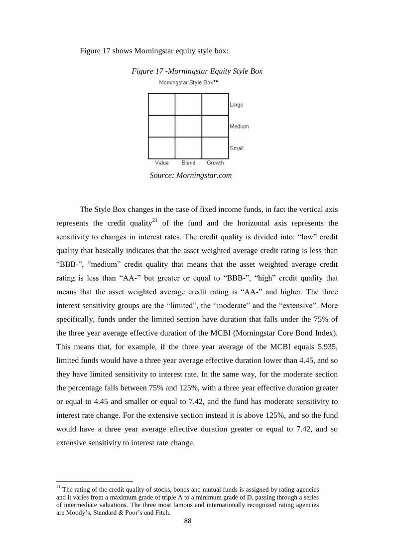
88
Figure 17 shows Morningstar equity style box:
Figure 17 -Morningstar Equity Style Box
Source: Morningstar.com
The Style Box changes in the case of fixed income funds, in fact the vertical axis
represents the credit quality21
of the fund and the horizontal axis represents the
sensitivity to changes in interest rates. The credit quality is divided into: ―low‖ credit
quality that basically indicates that the asset weighted average credit rating is less than
―BBB-‖, ―medium‖ credit quality that means that the asset weighted average credit
rating is less than ―AA-‖ but greater or equal to ―BBB-‖, ―high‖ credit quality that
means that the asset weighted average credit rating is ―AA-‖ and higher. The three
interest sensitivity groups are the ―limited‖, the ―moderate‖ and the ―extensive‖. More
specifically, funds under the limited section have duration that falls under the 75% of
the three year average effective duration of the MCBI (Morningstar Core Bond Index).
This means that, for example, if the three year average of the MCBI equals 5.935,
limited funds would have a three year average effective duration lower than 4.45, and so
they have limited sensitivity to interest rate. In the same way, for the moderate section
the percentage falls between 75% and 125%, with a three year effective duration greater
or equal to 4.45 and smaller or equal to 7.42, and the fund has moderate sensitivity to
interest rate change. For the extensive section instead it is above 125%, and so the fund
would have a three year average effective duration greater or equal to 7.42, and so
extensive sensitivity to interest rate change.
21
The rating of the credit quality of stocks, bonds and mutual funds is assigned by rating agencies
and it varies from a maximum grade of triple A to a minimum grade of D, passing through a series
of intermediate valuations. The three most famous and internationally recognized rating agencies
are Moody‘s, Standard & Poor‘s and Fitch.
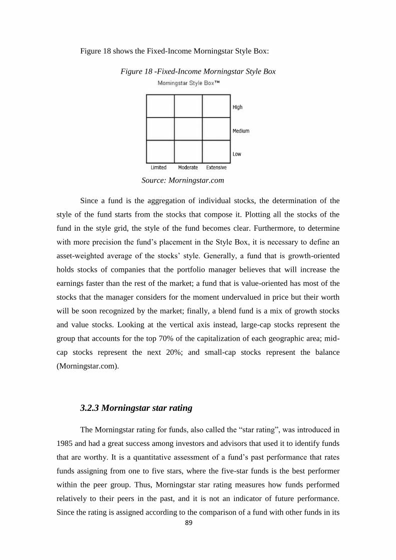
89
Figure 18 shows the Fixed-Income Morningstar Style Box:
Figure 18 -Fixed-Income Morningstar Style Box
Source: Morningstar.com
Since a fund is the aggregation of individual stocks, the determination of the
style of the fund starts from the stocks that compose it. Plotting all the stocks of the
fund in the style grid, the style of the fund becomes clear. Furthermore, to determine
with more precision the fund‘s placement in the Style Box, it is necessary to define an
asset-weighted average of the stocks‘ style. Generally, a fund that is growth-oriented
holds stocks of companies that the portfolio manager believes that will increase the
earnings faster than the rest of the market; a fund that is value-oriented has most of the
stocks that the manager considers for the moment undervalued in price but their worth
will be soon recognized by the market; finally, a blend fund is a mix of growth stocks
and value stocks. Looking at the vertical axis instead, large-cap stocks represent the
group that accounts for the top 70% of the capitalization of each geographic area; mid-
cap stocks represent the next 20%; and small-cap stocks represent the balance
(Morningstar.com).
3.2.3 Morningstar star rating
The Morningstar rating for funds, also called the ―star rating‖, was introduced in
1985 and had a great success among investors and advisors that used it to identify funds
that are worthy. It is a quantitative assessment of a fund‘s past performance that rates
funds assigning from one to five stars, where the five-star funds is the best performer
within the peer group. Thus, Morningstar star rating measures how funds performed
relatively to their peers in the past, and it is not an indicator of future performance.
Since the rating is assigned according to the comparison of a fund with other funds in its
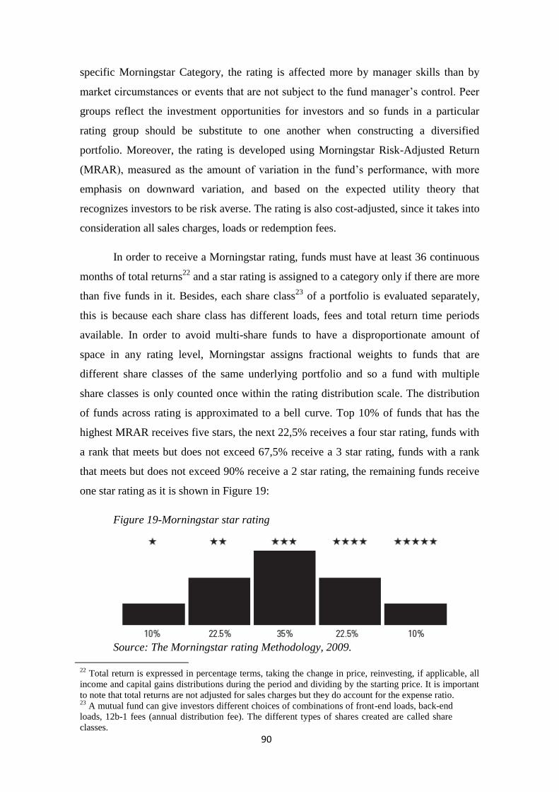
90
specific Morningstar Category, the rating is affected more by manager skills than by
market circumstances or events that are not subject to the fund manager‘s control. Peer
groups reflect the investment opportunities for investors and so funds in a particular
rating group should be substitute to one another when constructing a diversified
portfolio. Moreover, the rating is developed using Morningstar Risk-Adjusted Return
(MRAR), measured as the amount of variation in the fund‘s performance, with more
emphasis on downward variation, and based on the expected utility theory that
recognizes investors to be risk averse. The rating is also cost-adjusted, since it takes into
consideration all sales charges, loads or redemption fees.
In order to receive a Morningstar rating, funds must have at least 36 continuous
months of total returns22
and a star rating is assigned to a category only if there are more
than five funds in it. Besides, each share class23
of a portfolio is evaluated separately,
this is because each share class has different loads, fees and total return time periods
available. In order to avoid multi-share funds to have a disproportionate amount of
space in any rating level, Morningstar assigns fractional weights to funds that are
different share classes of the same underlying portfolio and so a fund with multiple
share classes is only counted once within the rating distribution scale. The distribution
of funds across rating is approximated to a bell curve. Top 10% of funds that has the
highest MRAR receives five stars, the next 22,5% receives a four star rating, funds with
a rank that meets but does not exceed 67,5% receive a 3 star rating, funds with a rank
that meets but does not exceed 90% receive a 2 star rating, the remaining funds receive
one star rating as it is shown in Figure 19:
Figure 19-Morningstar star rating
Source: The Morningstar rating Methodology, 2009.
22
Total return is expressed in percentage terms, taking the change in price, reinvesting, if applicable, all
income and capital gains distributions during the period and dividing by the starting price. It is important
to note that total returns are not adjusted for sales charges but they do account for the expense ratio. 23
A mutual fund can give investors different choices of combinations of front-end loads, back-end
loads, 12b-1 fees (annual distribution fee). The different types of shares created are called share
classes.
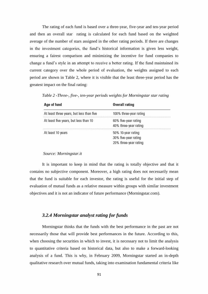
91
The rating of each fund is based over a three-year, five-year and ten-year period
and then an overall star rating is calculated for each fund based on the weighted
average of the number of stars assigned in the other rating periods. If there are changes
in the investment categories, the fund‘s historical information is given less weight,
ensuring a fairest comparison and minimizing the incentive for fund companies to
change a fund‘s style in an attempt to receive a better rating. If the fund maintained its
current category over the whole period of evaluation, the weights assigned to each
period are shown in Table 2, where it is visible that the least three-year period has the
greatest impact on the final rating:
Table 2 -Three-, five-, ten-year periods weights for Morningstar star rating
Source: Morningstar.it
It is important to keep in mind that the rating is totally objective and that it
contains no subjective component. Moreover, a high rating does not necessarily mean
that the fund is suitable for each investor, the rating is useful for the initial step of
evaluation of mutual funds as a relative measure within groups with similar investment
objectives and it is not an indicator of future performance (Morningstar.com).
3.2.4 Morningstar analyst rating for funds
Morningstar thinks that the funds with the best performance in the past are not
necessarily those that will provide best performances in the future. According to this,
when choosing the securities in which to invest, it is necessary not to limit the analysis
to quantitative criteria based on historical data, but also to make a forward-looking
analysis of a fund. This is why, in February 2009, Morningstar started an in-depth
qualitative research over mutual funds, taking into examination fundamental criteria like
92
costs, the experience of the fund manager, the management team and the strategy of the
investment.
Morningstar qualitative analysis is based on 5 pillars: people, process,
performance, parent and price. For each of these pillars Morningstar collects
information through its data bank, other instruments for the analysis developed by the
company itself, questionnaires sent to the management of the investment management
companies and direct meetings with fund managers to deepen the knowledge of the
fund. The final judgment, that is reviewed on a semester basis, is developed in the
European Committee of rating, that assures the homogeneity in the application of the
methodology of evaluation.
Relative to ―people‖, the aspects taken into consideration are the competencies,
the experience, the temperament and the internal organization of the team of investment,
with the verification of the adequacy with the strategy of investment. The study of the
―process‖ focuses on the coherence between the philosophy of the investment and the
mechanism of selection of the stocks and studies whether the management has a
competitive advantage that enables to execute the process well and consistently over
time. Particular attention is devoted to risks, in terms of geographical concentration,
business sector and style of investment. The analysis of the ―performance‖ focuses on
identifying how the strategy of the fund is translated into results for the investors. This
means that it measures the consistency of the investment, of returns and of the risk with
the strategy of investment declared. The pillar about ―parent‖ focuses on the legal
person that promotes the fund. The organizing structure, the available resources, the
remuneration policy and the culture (what priorities prevail, like the policy of selling,
salesmanship, or that of providing an excellent service, stewardship) are factors that
influence the choice of the management of the fund. Lastly, the pillar of ―price‖, refers
to the examination of the costs of the fund compared to similar funds sold through
similar channels. This element is very important, it presents low uncertainty and
consistently influences the future performance.
The qualitative rating by Morningstar released on the basis of the five-tier
judgments, is composed of three positive grades that are Gold, Silver and Bronze, a
Neutral grade, and a Negative grade, based on the analyst conviction in the fund‘s
ability to outperform its peer group and/or relevant benchmark on a risk-adjusted basis
93
over the long term. Let us describe the features of each evaluation of the qualitative
rating:
Gold, the best-of-breed fund that distinguishes itself across the five pillars and
gained the analyst‘s higher level of conviction;
Silver, assigned to a fund whose advantages outweigh the disadvantages across
the five pillars and gained a sufficient level of analyst conviction to be granted a
positive rating;
Bronze, for a fund that has advantages across several, but not all, pillars, and the
strengths of the fund give to the analyst a certain level of conviction;
Neutral, assigned to a fund that does not deliver exceptional returns but it is not
likely to significantly underperform, according to analysts;
Negative, for a fund that has at least one flaw that is likely to significantly
obstacle a good performance and is considered to be an inferior opportunity with
respect to its peers.
Morningstar does not receive any payment from the fund management society
neither to provide the rating nor to produce the research report and it points at
furnishing information independent to investors and consultants. The decision to
produce a report over a particular fund is the fruit of the discretion of Morningstar
analysts and of the interest expressed by investors.
Another interesting project by Morningstar is that of honoring managers, funds,
fund managers and fund groups throughout the year with a series of awards known as
―The Morningstar Awards‖, given to those that outperformed competition over one,
three and five periods. Examples are the award introduced in 2000 of the ―CEO of the
Year‖ where Morningstar recognizes the chief executive that demonstrates independent
thinking, creates value for the shareholders and generally distinguishes with respect to
others. Another important award is the ―Fund Manager of the Year‖, established in
1988, recognized to the portfolio manager that demonstrates excellent investment skills
measured by the returns of the year and the long-term risk-adjusted performance
(Morningstar.com).

94
3.3 Clerical Medical Managed funds by Morningstar Investment
Management
3.3.1 Clerical Medical, the company
Clerical Medical is a British company specialized in insurance and financial
products and it is part of the Lloyds Banking Group. The birth of Clerical Medical dates
back to 1824, when a group of friends met in ―The Freemason‘s Tavern‖, a tavern in
London. The innovative idea of the group was to propose financial products specific to
members of the clergy and doctors, and from this it takes the name. No other financial
insurance company in fact wanted to insure these two categories of professionals
because of their life style. After almost two hundred years from its birth, Clerical
Medical became part of the Lloyds Banking Group, one of the greatest providers of
financial services in the United Kingdom.
In Italy, Clerical Medical opened its first office in 2002 and its main business is
in insurance investment instruments. It operates in the Italian territory with multi
manager instruments that are distributed by partner independent intermediaries.
Products offered by Clerical Medical are mainly insurance and financial instruments, of
the type unit-linked through a one-time lump sum investment or a systematic investment
plan. These products allow to invest in a wide range of internal funds.
Table 3 contains the list of the 40 internal funds of Clerical Medical divided into
open-end funds and closed-end funds.
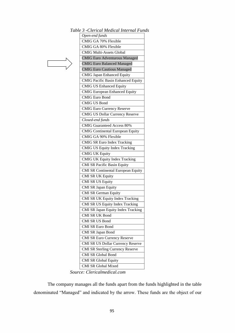
95
Table 3 -Clerical Medical Internal Funds Open-end funds
CMIG GA 70% Flexible
CMIG GA 80% Flexible
CMIG Multi-Assets Global
CMIG Euro Adventurous Managed
CMIG Euro Balanced Managed
CMIG Euro Cautious Managed
CMIG Japan Enhanced Equity
CMIG Pacific Basin Enhanced Equity
CMIG US Enhanced Equity
CMIG European Enhanced Equity
CMIG Euro Bond
CMIG US Bond
CMIG Euro Currency Reserve
CMIG US Dollar Currency Reserve
Closed-end funds
CMIG Guaranteed Access 80%
CMIG Continental European Equity
CMIG GA 90% Flexible
CMIG SR Euro Index Tracking
CMIG US Equity Index Tracking
CMIG UK Equity
CMIG UK Equity Index Tracking
CMI SR Pacific Basin Equity
CMI SR Continental European Equity
CMI SR UK Equity
CMI SR US Equity
CMI SR Japan Equity
CMI SR German Equity
CMI SR UK Equity Index Tracking
CMI SR US Equity Index Tracking
CMI SR Japan Equity Index Tracking
CMI SR UK Bond
CMI SR US Bond
CMI SR Euro Bond
CMI SR Japan Bond
CMI SR Euro Currency Reserve
CMI SR US Dollar Currency Reserve
CMI SR Sterling Currency Reserve
CMI SR Global Bond
CMI SR Global Equity
CMI SR Global Mixed
Source: Clericalmedical.com
The company manages all the funds apart from the funds highlighted in the table
denominated ―Managed‖ and indicated by the arrow. These funds are the object of our
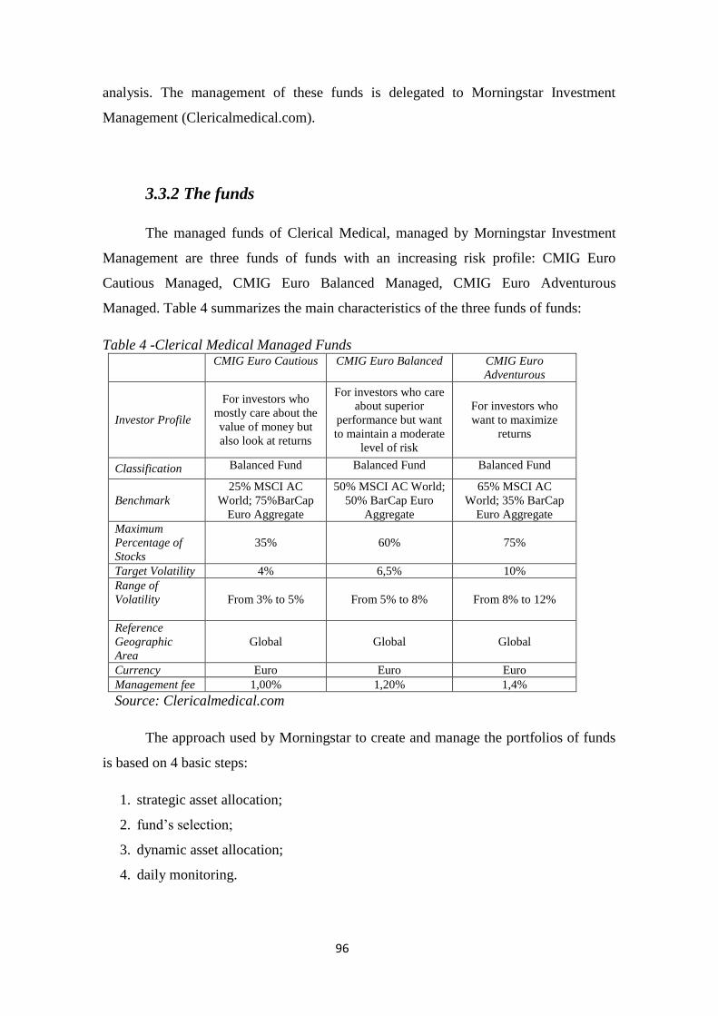
96
analysis. The management of these funds is delegated to Morningstar Investment
Management (Clericalmedical.com).
3.3.2 The funds
The managed funds of Clerical Medical, managed by Morningstar Investment
Management are three funds of funds with an increasing risk profile: CMIG Euro
Cautious Managed, CMIG Euro Balanced Managed, CMIG Euro Adventurous
Managed. Table 4 summarizes the main characteristics of the three funds of funds:
Table 4 -Clerical Medical Managed Funds CMIG Euro Cautious CMIG Euro Balanced CMIG Euro
Adventurous
Investor Profile
For investors who
mostly care about the
value of money but
also look at returns
For investors who care
about superior
performance but want
to maintain a moderate
level of risk
For investors who
want to maximize
returns
Classification Balanced Fund Balanced Fund Balanced Fund
Benchmark
25% MSCI AC
World; 75%BarCap
Euro Aggregate
50% MSCI AC World;
50% BarCap Euro
Aggregate
65% MSCI AC
World; 35% BarCap
Euro Aggregate
Maximum
Percentage of
Stocks
35% 60% 75%
Target Volatility 4% 6,5% 10%
Range of
Volatility
From 3% to 5% From 5% to 8% From 8% to 12%
Reference
Geographic
Area
Global Global Global
Currency Euro Euro Euro
Management fee 1,00% 1,20% 1,4%
Source: Clericalmedical.com
The approach used by Morningstar to create and manage the portfolios of funds
is based on 4 basic steps:
1. strategic asset allocation;
2. fund‘s selection;
3. dynamic asset allocation;
4. daily monitoring.
97
We will now concentrate on Morningstar‘s strategy developed to create the three
portfolios of funds and focus on its distinctive features.
3.3.3 Morningstar strategic asset allocation
Morningstar strategic asset allocation starts with a reference portfolio where the
management team decides in which asset classes to invest: for example equity Europe,
equity North America, bond Europe, bond Emerging markets and so on. Once the asset
classes are chosen, assumptions over risk and return are made and an optimization
process is run in order to find the efficient frontier of portfolios. This is mainly what
every institutional investor does. The greatness of Morningstar lies in the fact that every
solution is highly customized and is elaborated step by step together with the client that
in our case is the insurance company Clerical Medical and so the three portfolios of
funds are created for a typical Clerical Medical client.
Morningstar believes that it does not exist a single model that is able to catch the
complexity of the world and of financial markets and so it uses different approaches and
different models and compares them. Examples are econometric models that study the
actual economic conditions of the market (tax of growth of the economy, inflation and
interest rates) to delineate the expected future macroeconomic scenario, but also the
internal rate of return and the ―views‖ of money managers over asset returns. After the
comparison of all the approaches, it runs the optimization process.
3.3.3.1 Markowitz 2.0
Morningstar optimization model is called Markowitz 2.0. The model is
explained in a book by Kaplan (2011), one of the main experts behind the elaboration of
the Morningstar rating and the Morningstar Style Box. In his book ―Frontiers of modern
asset allocation‖ (Kaplan, 2011), Kaplan compares the Wright Brothers to Markowitz:
the formers pioneered powered flight in 1903, while the latter pioneered the modern
portfolio theory. The genius of the Wright Brothers lays in conquering the three axes of
control: pitch, yaw and roll; the genius of Markowitz instead is based on the three
principles of risk, reward and correlation among the assets in a portfolio. However,
while the technology of aircraft has developed so much over the years that Wright‘s
98
original plane is hardly recognizable, the portfolio optimization model has not evolved
that much, although in a scenario where technologies are advancing incredibly and
market crashed. As Kaplan says, after the crash of 2008 and the skepticism of investors
towards financial markets, it was the perfect time to define a model built on the
fundamentals of Markowitz, but with several developments. The final model, developed
by taking advantage of the latest in economic thoughts and computer technology, is
dubbed Markowitz 2.0.
Markowitz 2.0 is suitable to the twenty-first century financial markets, financial
instruments and concerns of investors and it discusses five main enhancements:
1. the scenario considers fat-tailed24
distribution;
2. the single period expected return is substituted with the long-term forward-
looking geometric mean that takes into account the accumulation of wealth;
3. standard deviation is substituted with conditional value at risk;
4. the covariance matrix is substituted with a Monte Carlo simulation that
incorporates any distribution;
5. the technologies pioneered by Savage (2009) in probability management are
exploited.
Let us analyze each point in more detail. First, we know that under the mean-
variance optimization model, the distribution of returns is assumed to be a symmetrical
bell-shaped curve. Kaplan criticizes this approach stating that in reality asset returns do
not always follow a symmetrical bell-shaped curve and the distribution might be skewed
to left or right, with skinnier or fatter tails.
Figure 20 shows the distribution of returns from 1996 to 2008 of different asset
classes: it is evident that returns are skewed and do not always follow a bell-shaped
distribution.
24
Probability distribution that exhibits large Skewness and Kurtosis (See Note 25 for more details).
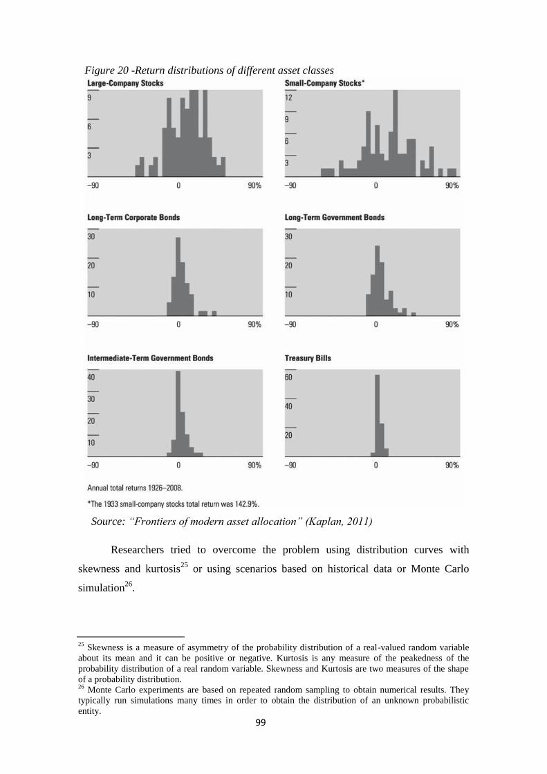
99
Figure 20 -Return distributions of different asset classes
Source: “Frontiers of modern asset allocation” (Kaplan, 2011)
Researchers tried to overcome the problem using distribution curves with
skewness and kurtosis25
or using scenarios based on historical data or Monte Carlo
simulation26
.
25
Skewness is a measure of asymmetry of the probability distribution of a real-valued random variable
about its mean and it can be positive or negative. Kurtosis is any measure of the peakedness of the
probability distribution of a real random variable. Skewness and Kurtosis are two measures of the shape
of a probability distribution. 26
Monte Carlo experiments are based on repeated random sampling to obtain numerical results. They
typically run simulations many times in order to obtain the distribution of an unknown probabilistic
entity.
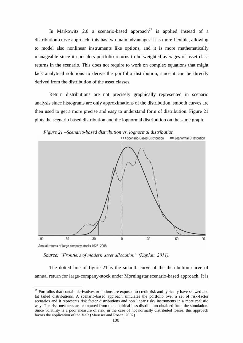
100
In Markowitz 2.0 a scenario-based approach27
is applied instead of a
distribution-curve approach; this has two main advantages: it is more flexible, allowing
to model also nonlinear instruments like options, and it is more mathematically
manageable since it considers portfolio returns to be weighted averages of asset-class
returns in the scenario. This does not require to work on complex equations that might
lack analytical solutions to derive the portfolio distribution, since it can be directly
derived from the distribution of the asset classes.
Return distributions are not precisely graphically represented in scenario
analysis since histograms are only approximations of the distribution, smooth curves are
then used to get a more precise and easy to understand form of distribution. Figure 21
plots the scenario based distribution and the lognormal distribution on the same graph.
Figure 21 –Scenario-based distribution vs. lognormal distribution
Source: “Frontiers of modern asset allocation” (Kaplan, 2011).
The dotted line of figure 21 is the smooth curve of the distribution curve of
annual return for large-company-stock under Morningstar scenario-based approach. It is
27
Portfolios that contain derivatives or options are exposed to credit risk and typically have skewed and
fat tailed distributions. A scenario-based approach simulates the portfolio over a set of risk-factor
scenarios and it represents risk factor distributions and non linear risky instruments in a more realistic
way. The risk measures are computed from the empirical loss distribution obtained from the simulation.
Since volatility is a poor measure of risk, in the case of not normally distributed losses, this approach
favors the application of the VaR (Mausser and Rosen, 2002).
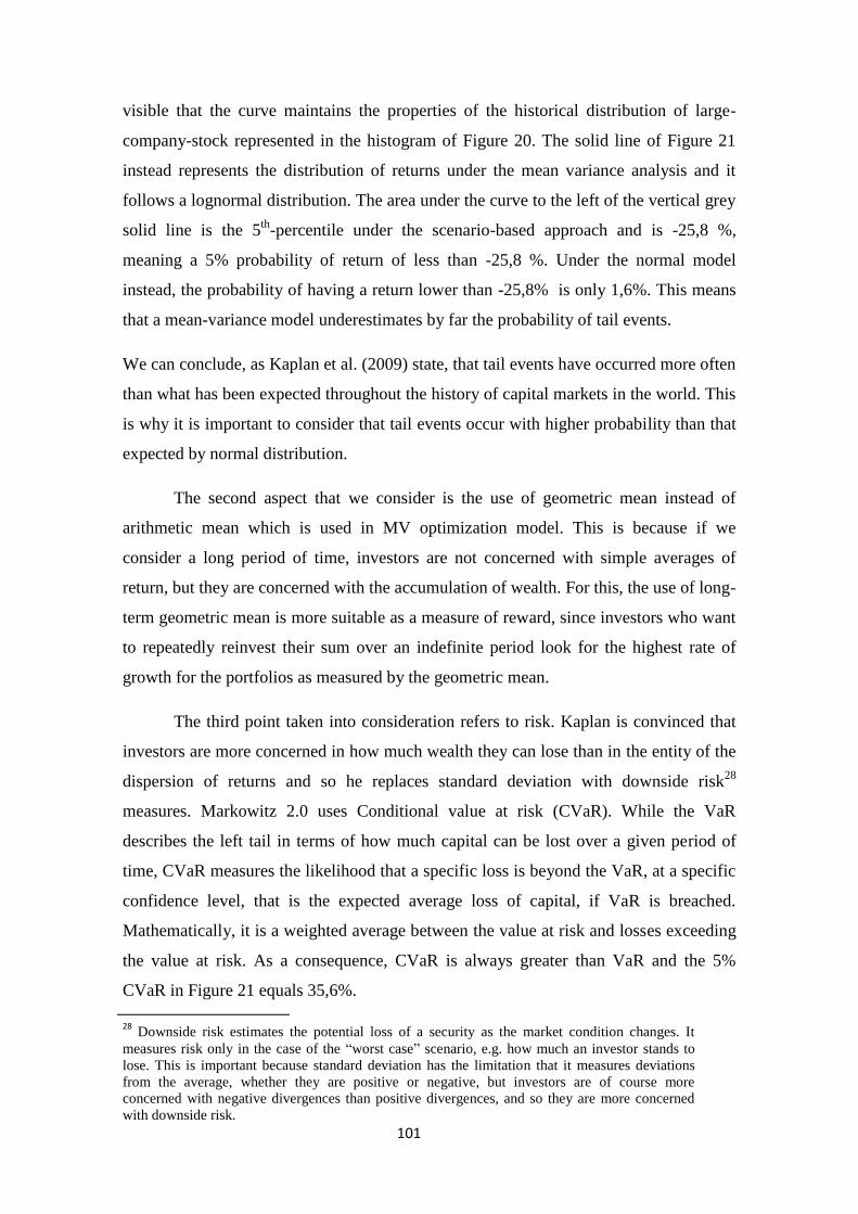
101
visible that the curve maintains the properties of the historical distribution of large-
company-stock represented in the histogram of Figure 20. The solid line of Figure 21
instead represents the distribution of returns under the mean variance analysis and it
follows a lognormal distribution. The area under the curve to the left of the vertical grey
solid line is the 5th
-percentile under the scenario-based approach and is -25,8 %,
meaning a 5% probability of return of less than -25,8 %. Under the normal model
instead, the probability of having a return lower than -25,8% is only 1,6%. This means
that a mean-variance model underestimates by far the probability of tail events.
We can conclude, as Kaplan et al. (2009) state, that tail events have occurred more often
than what has been expected throughout the history of capital markets in the world. This
is why it is important to consider that tail events occur with higher probability than that
expected by normal distribution.
The second aspect that we consider is the use of geometric mean instead of
arithmetic mean which is used in MV optimization model. This is because if we
consider a long period of time, investors are not concerned with simple averages of
return, but they are concerned with the accumulation of wealth. For this, the use of long-
term geometric mean is more suitable as a measure of reward, since investors who want
to repeatedly reinvest their sum over an indefinite period look for the highest rate of
growth for the portfolios as measured by the geometric mean.
The third point taken into consideration refers to risk. Kaplan is convinced that
investors are more concerned in how much wealth they can lose than in the entity of the
dispersion of returns and so he replaces standard deviation with downside risk28
measures. Markowitz 2.0 uses Conditional value at risk (CVaR). While the VaR
describes the left tail in terms of how much capital can be lost over a given period of
time, CVaR measures the likelihood that a specific loss is beyond the VaR, at a specific
confidence level, that is the expected average loss of capital, if VaR is breached.
Mathematically, it is a weighted average between the value at risk and losses exceeding
the value at risk. As a consequence, CVaR is always greater than VaR and the 5%
CVaR in Figure 21 equals 35,6%.
28
Downside risk estimates the potential loss of a security as the market condition changes. It
measures risk only in the case of the ―worst case‖ scenario, e.g. how much an investor stands to
lose. This is important because standard deviation has the limitation that it measures deviations
from the average, whether they are positive or negative, but investors are of course more
concerned with negative divergences than positive divergences, and so they are more concerned
with downside risk.

102
The fourth point modified in Markowitz 2.0 model is the correlation coefficient
used to measure the pair-wise co-variation. As we have already seen in Chapter 2, pair-
wise co-variation is not a good measure in particular in case of a global crisis, when all
major markets move down together. Morningstar scenario-based approach models
returns as moving apart from each other in scenarios that represent normal times, while
it models returns as moving downward together in scenarios that represent global crises.
Finally, Markowitz 2.0 uses the new technology of probability management
which extends data management to probability distribution. Savage invented the
Distribution String that is the main component of probability management and it
encloses thousands of trials as a single data element, eliminating the disadvantage of
storing and processing large amounts of data. Savage‘s Distribution String in fact
contains thousands of trials of a single data element but it takes an incredibly short
processing time and it allows to save on storage. Moreover, it is an interactive
simulation technology and provides a deep intuition into the sensitivity of each
portfolio, extreme events and black swans29
. Since scenario-based approach requires a
large amount of data to represent the thousands of scenarios that model returns and to
manage the data, Morningstar uses this technology.
Putting the five enhancements together, a new efficient frontier is obtained in the
geometric mean-CVaR set. Kaplan believes that this new efficient frontier is more
relevant to investors than the traditional one because it shows the tradeoff between risk
and return that really concerns investors. To sum up, this is a representation of long-
term potential growth versus short term potential loss.
29
The term black swan takes its name from Taleb (2004) who defined extreme events that have never
occurred before with this name.
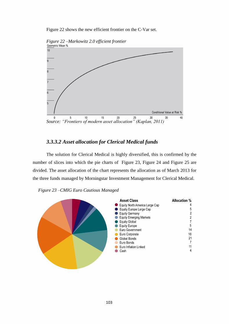
103
Figure 22 shows the new efficient frontier on the C-Var set.
Figure 22 –Markowitz 2.0 efficient frontier
Source: “Frontiers of modern asset allocation” (Kaplan, 2011)
3.3.3.2 Asset allocation for Clerical Medical funds
The solution for Clerical Medical is highly diversified, this is confirmed by the
number of slices into which the pie charts of Figure 23, Figure 24 and Figure 25 are
divided. The asset allocation of the chart represents the allocation as of March 2013 for
the three funds managed by Morningstar Investment Management for Clerical Medical.
Figure 23 –CMIG Euro Cautious Managed
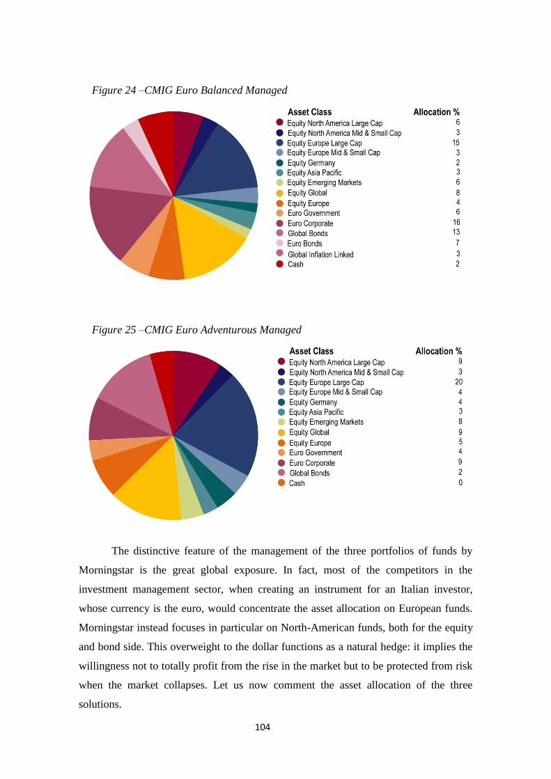
104
Figure 24 –CMIG Euro Balanced Managed
Figure 25 –CMIG Euro Adventurous Managed
The distinctive feature of the management of the three portfolios of funds by
Morningstar is the great global exposure. In fact, most of the competitors in the
investment management sector, when creating an instrument for an Italian investor,
whose currency is the euro, would concentrate the asset allocation on European funds.
Morningstar instead focuses in particular on North-American funds, both for the equity
and bond side. This overweight to the dollar functions as a natural hedge: it implies the
willingness not to totally profit from the rise in the market but to be protected from risk
when the market collapses. Let us now comment the asset allocation of the three
solutions.
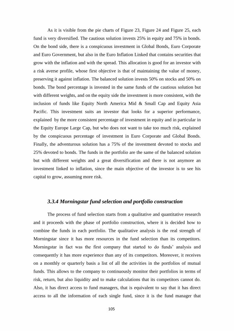
105
As it is visible from the pie charts of Figure 23, Figure 24 and Figure 25, each
fund is very diversified. The cautious solution invests 25% in equity and 75% in bonds.
On the bond side, there is a conspicuous investment in Global Bonds, Euro Corporate
and Euro Government, but also in the Euro Inflation Linked that contains securities that
grow with the inflation and with the spread. This allocation is good for an investor with
a risk averse profile, whose first objective is that of maintaining the value of money,
preserving it against inflation. The balanced solution invests 50% on stocks and 50% on
bonds. The bond percentage is invested in the same funds of the cautious solution but
with different weights, and on the equity side the investment is more consistent, with the
inclusion of funds like Equity North America Mid & Small Cap and Equity Asia
Pacific. This investment suits an investor that looks for a superior performance,
explained by the more consistent percentage of investment in equity and in particular in
the Equity Europe Large Cap, but who does not want to take too much risk, explained
by the conspicuous percentage of investment in Euro Corporate and Global Bonds.
Finally, the adventurous solution has a 75% of the investment devoted to stocks and
25% devoted to bonds. The funds in the portfolio are the same of the balanced solution
but with different weights and a great diversification and there is not anymore an
investment linked to inflation, since the main objective of the investor is to see his
capital to grow, assuming more risk.
3.3.4 Morningstar fund selection and portfolio construction
The process of fund selection starts from a qualitative and quantitative research
and it proceeds with the phase of portfolio construction, where it is decided how to
combine the funds in each portfolio. The qualitative analysis is the real strength of
Morningstar since it has more resources in the fund selection than its competitors.
Morningstar in fact was the first company that started to do funds‘ analysis and
consequently it has more experience than any of its competitors. Moreover, it receives
on a monthly or quarterly basis a list of all the activities in the portfolios of mutual
funds. This allows to the company to continuously monitor their portfolios in terms of
risk, return, but also liquidity and to make calculations that its competitors cannot do.
Also, it has direct access to fund managers, that is equivalent to say that it has direct
access to all the information of each single fund, since it is the fund manager that
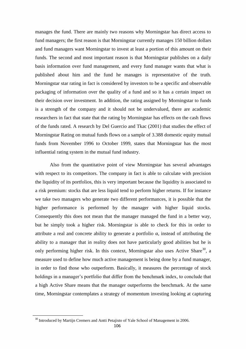
106
manages the fund. There are mainly two reasons why Morningstar has direct access to
fund managers; the first reason is that Morningstar currently manages 150 billion dollars
and fund managers want Morningstar to invest at least a portion of this amount on their
funds. The second and most important reason is that Morningstar publishes on a daily
basis information over fund management, and every fund manager wants that what is
published about him and the fund he manages is representative of the truth.
Morningstar star rating in fact is considered by investors to be a specific and observable
packaging of information over the quality of a fund and so it has a certain impact on
their decision over investment. In addition, the rating assigned by Morningstar to funds
is a strength of the company and it should not be undervalued, there are academic
researchers in fact that state that the rating by Morningstar has effects on the cash flows
of the funds rated. A research by Del Guercio and Tkac (2001) that studies the effect of
Morningstar Rating on mutual funds flows on a sample of 3.388 domestic equity mutual
funds from November 1996 to October 1999, states that Morningstar has the most
influential rating system in the mutual fund industry.
Also from the quantitative point of view Morningstar has several advantages
with respect to its competitors. The company in fact is able to calculate with precision
the liquidity of its portfolios, this is very important because the liquidity is associated to
a risk premium: stocks that are less liquid tend to perform higher returns. If for instance
we take two managers who generate two different performances, it is possible that the
higher performance is performed by the manager with higher liquid stocks.
Consequently this does not mean that the manager managed the fund in a better way,
but he simply took a higher risk. Morningstar is able to check for this in order to
attribute a real and concrete ability to generate a portfolio α, instead of attributing the
ability to a manager that in reality does not have particularly good abilities but he is
only performing higher risk. In this context, Morningstar also uses Active Share30
, a
measure used to define how much active management is being done by a fund manager,
in order to find those who outperform. Basically, it measures the percentage of stock
holdings in a manager‘s portfolio that differ from the benchmark index, to conclude that
a high Active Share means that the manager outperforms the benchmark. At the same
time, Morningstar contemplates a strategy of momentum investing looking at capturing
30
Introduced by Martijn Cremers and Antti Petajisto of Yale School of Management in 2006.

107
gains by riding ―hot‖ stocks and selling ―cold‖ ones through detailed study of the stocks
that it takes into consideration for its portfolio construction.
Quantitative measures have a great importance, however, in the phase of
portfolio construction, Morningstar devotes great attention to the experience of the
people that make the investment, e.g. the fund managers. The aim is that of creating a
portfolio with the maximum diversification possible and for this, when associating
funds to construct a portfolio, the company considers all the variables that characterize
the fund, starting from the fund manager himself. Morningstar studies the past career of
portfolio managers: every portfolio manager usually starts his career as a portfolio
analyst and tends to concentrate on one or two business sectors maximum, like, for
example, the pharmaceuticals and the financial. So, once he becomes a fund manager,
he would tend to concentrate on these sectors, where he can make a difference and
perform better than his competitors, meaning that he has a competitive advantage. This
is what Morningstar aims at: the creation of a portfolio that combines managers with
different abilities and competences in different business sectors to create a portfolio that
has a competitive advantage.
In its strategy of portfolio construction, Morningstar does not only consider the
complementarities among the different asset classes and the different strategies, but it
also makes sure that there is no overlapping of stocks over the different styles once the
funds are aggregated in a portfolio. Figure 26 represents a Morningstar style box that
aggregates three equity funds that visibly have different styles, to create an example of a
diversified portfolio. What Morningstar tries to do, is to create the most diversified
portfolio from the point of view of the style and it does not choose funds with
overlapping styles. In the example of Figure 26, Equity Fund 1invests in stocks with
high capitalization, Equity Fund 2 invests in stocks with medium capitalization and
Equity Fund 3 invests in stocks with small capitalization. The combination of these
three funds ends up to be a very diversified portfolio of funds that spreads over all the
styles. Again, Morningstar has the advantage of having direct access to all the
information that its competitors do not immediately have.
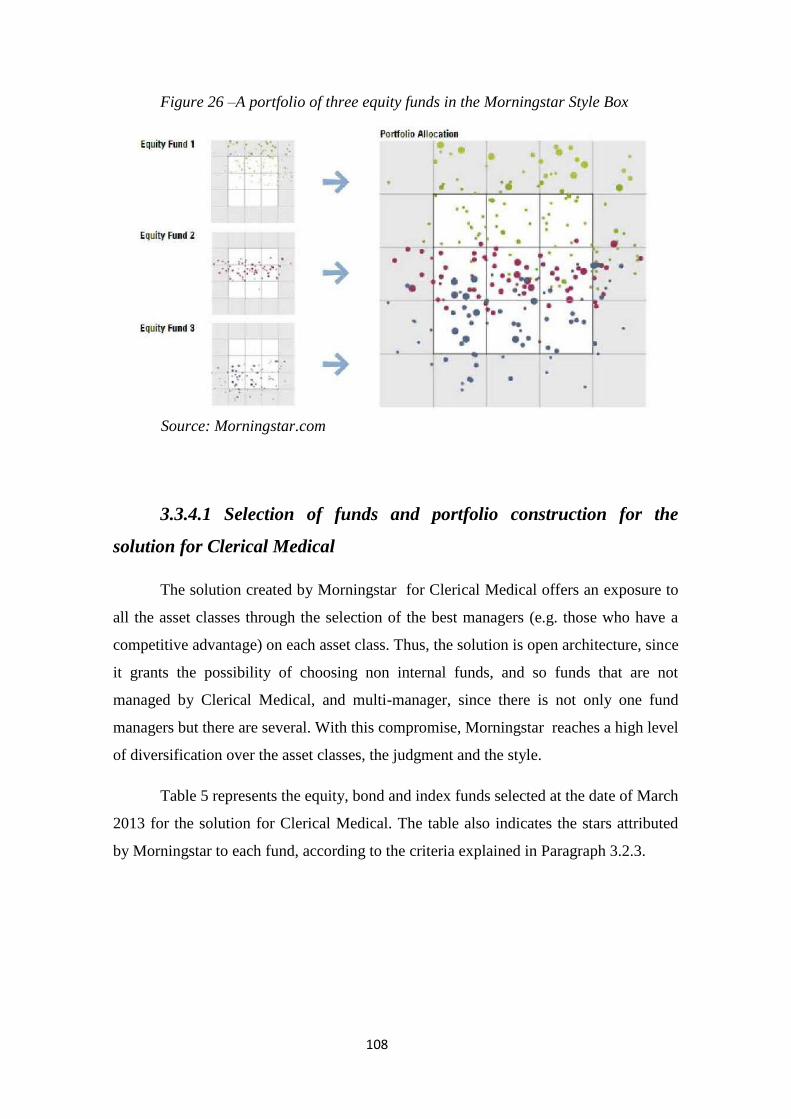
108
Figure 26 –A portfolio of three equity funds in the Morningstar Style Box
Source: Morningstar.com
3.3.4.1 Selection of funds and portfolio construction for the
solution for Clerical Medical
The solution created by Morningstar for Clerical Medical offers an exposure to
all the asset classes through the selection of the best managers (e.g. those who have a
competitive advantage) on each asset class. Thus, the solution is open architecture, since
it grants the possibility of choosing non internal funds, and so funds that are not
managed by Clerical Medical, and multi-manager, since there is not only one fund
managers but there are several. With this compromise, Morningstar reaches a high level
of diversification over the asset classes, the judgment and the style.
Table 5 represents the equity, bond and index funds selected at the date of March
2013 for the solution for Clerical Medical. The table also indicates the stars attributed
by Morningstar to each fund, according to the criteria explained in Paragraph 3.2.3.
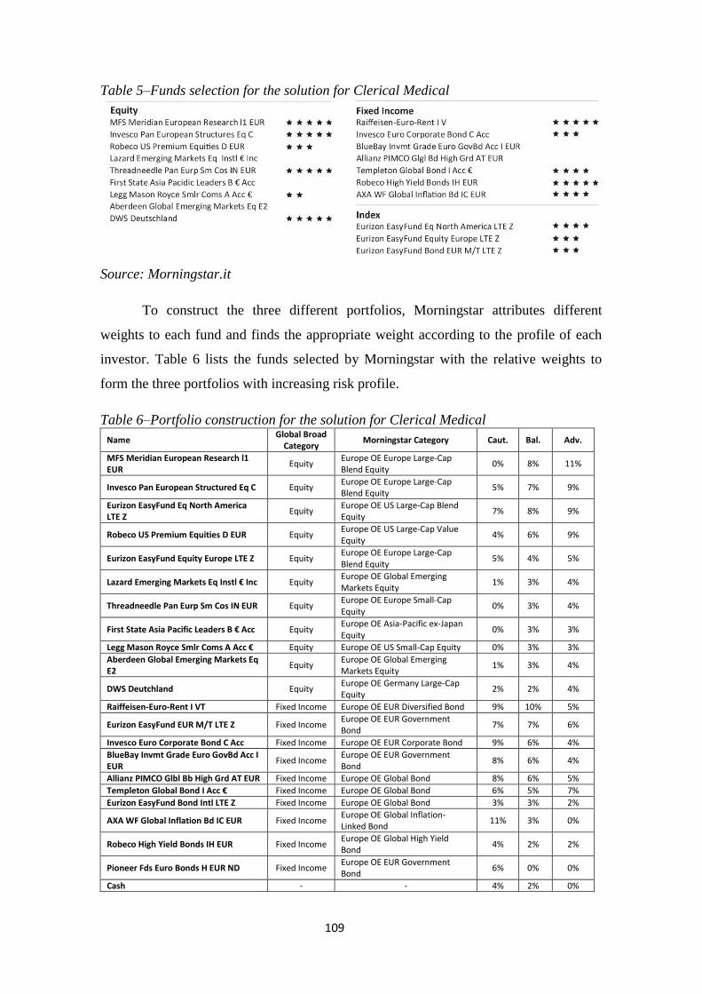
109
Table 5–Funds selection for the solution for Clerical Medical
Source: Morningstar.it
To construct the three different portfolios, Morningstar attributes different
weights to each fund and finds the appropriate weight according to the profile of each
investor. Table 6 lists the funds selected by Morningstar with the relative weights to
form the three portfolios with increasing risk profile.
Table 6–Portfolio construction for the solution for Clerical Medical
Name Global Broad
Category Morningstar Category Caut. Bal. Adv.
MFS Meridian European Research l1 EUR
Equity Europe OE Europe Large-Cap Blend Equity
0% 8% 11%
Invesco Pan European Structured Eq C Equity Europe OE Europe Large-Cap Blend Equity
5% 7% 9%
Eurizon EasyFund Eq North America LTE Z
Equity Europe OE US Large-Cap Blend Equity
7% 8% 9%
Robeco US Premium Equities D EUR Equity Europe OE US Large-Cap Value Equity
4% 6% 9%
Eurizon EasyFund Equity Europe LTE Z Equity Europe OE Europe Large-Cap Blend Equity
5% 4% 5%
Lazard Emerging Markets Eq Instl € Inc Equity Europe OE Global Emerging Markets Equity
1% 3% 4%
Threadneedle Pan Eurp Sm Cos IN EUR Equity Europe OE Europe Small-Cap Equity
0% 3% 4%
First State Asia Pacific Leaders B € Acc Equity Europe OE Asia-Pacific ex-Japan Equity
0% 3% 3%
Legg Mason Royce Smlr Coms A Acc € Equity Europe OE US Small-Cap Equity 0% 3% 3%
Aberdeen Global Emerging Markets Eq E2
Equity Europe OE Global Emerging Markets Equity
1% 3% 4%
DWS Deutchland Equity Europe OE Germany Large-Cap Equity
2% 2% 4%
Raiffeisen-Euro-Rent I VT Fixed Income Europe OE EUR Diversified Bond 9% 10% 5%
Eurizon EasyFund EUR M/T LTE Z Fixed Income Europe OE EUR Government Bond
7% 7% 6%
Invesco Euro Corporate Bond C Acc Fixed Income Europe OE EUR Corporate Bond 9% 6% 4%
BlueBay Invmt Grade Euro GovBd Acc I EUR
Fixed Income Europe OE EUR Government Bond
8% 6% 4%
Allianz PIMCO Glbl Bb High Grd AT EUR Fixed Income Europe OE Global Bond 8% 6% 5%
Templeton Global Bond I Acc € Fixed Income Europe OE Global Bond 6% 5% 7%
Eurizon EasyFund Bond Intl LTE Z Fixed Income Europe OE Global Bond 3% 3% 2%
AXA WF Global Inflation Bd IC EUR Fixed Income Europe OE Global Inflation-Linked Bond
11% 3% 0%
Robeco High Yield Bonds IH EUR Fixed Income Europe OE Global High Yield Bond
4% 2% 2%
Pioneer Fds Euro Bonds H EUR ND Fixed Income Europe OE EUR Government Bond
6% 0% 0%
Cash - - 4% 2% 0%
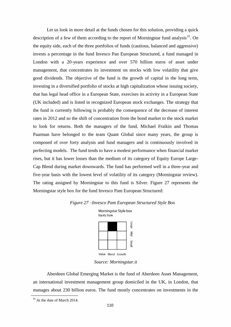
110
Let us look in more detail at the funds chosen for this solution, providing a quick
description of a few of them according to the report of Morningstar fund analysis31
. On
the equity side, each of the three portfolios of funds (cautious, balanced and aggressive)
invests a percentage in the fund Invesco Pan European Structured, a fund managed in
London with a 20-years experience and over 570 billion euros of asset under
management, that concentrates its investment on stocks with low volatility that give
good dividends. The objective of the fund is the growth of capital in the long term,
investing in a diversified portfolio of stocks at high capitalization whose issuing society,
that has legal head office in a European State, exercises its activity in a European State
(UK included) and is listed in recognized European stock exchanges. The strategy that
the fund is currently following is probably the consequence of the decrease of interest
rates in 2012 and so the shift of concentration from the bond market to the stock market
to look for returns. Both the managers of the fund, Michael Fraikin and Thomas
Paarman have belonged to the team Quant Global since many years, the group is
composed of over forty analysts and fund managers and is continuously involved in
perfecting models. The fund tends to have a modest performance when financial market
rises, but it has lower losses than the medium of its category of Equity Europe Large-
Cap Blend during market downwards. The fund has performed well in a three-year and
five-year basis with the lowest level of volatility of its category (Morningstar review).
The rating assigned by Morningstar to this fund is Silver. Figure 27 represents the
Morningstar style box for the fund Invesco Pam European Structured:
Figure 27 –Invesco Pam European Structured Style Box
Source: Morningstar.it
Aberdeen Global Emerging Market is the fund of Aberdeen Asset Management,
an international investment management group domiciled in the UK, in London, that
manages about 230 billion euros. The fund mostly concentrates on investments in the
31 At the date of March 2014.
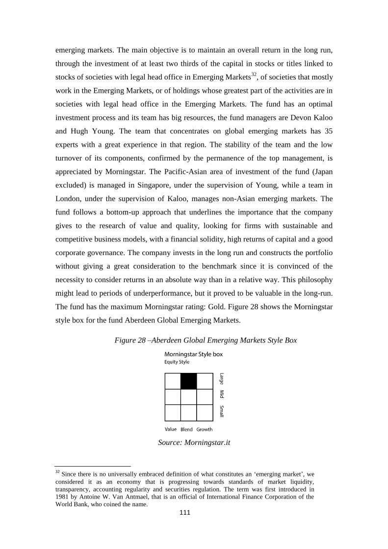
111
emerging markets. The main objective is to maintain an overall return in the long run,
through the investment of at least two thirds of the capital in stocks or titles linked to
stocks of societies with legal head office in Emerging Markets32
, of societies that mostly
work in the Emerging Markets, or of holdings whose greatest part of the activities are in
societies with legal head office in the Emerging Markets. The fund has an optimal
investment process and its team has big resources, the fund managers are Devon Kaloo
and Hugh Young. The team that concentrates on global emerging markets has 35
experts with a great experience in that region. The stability of the team and the low
turnover of its components, confirmed by the permanence of the top management, is
appreciated by Morningstar. The Pacific-Asian area of investment of the fund (Japan
excluded) is managed in Singapore, under the supervision of Young, while a team in
London, under the supervision of Kaloo, manages non-Asian emerging markets. The
fund follows a bottom-up approach that underlines the importance that the company
gives to the research of value and quality, looking for firms with sustainable and
competitive business models, with a financial solidity, high returns of capital and a good
corporate governance. The company invests in the long run and constructs the portfolio
without giving a great consideration to the benchmark since it is convinced of the
necessity to consider returns in an absolute way than in a relative way. This philosophy
might lead to periods of underperformance, but it proved to be valuable in the long-run.
The fund has the maximum Morningstar rating: Gold. Figure 28 shows the Morningstar
style box for the fund Aberdeen Global Emerging Markets.
Figure 28 –Aberdeen Global Emerging Markets Style Box
Source: Morningstar.it
32
Since there is no universally embraced definition of what constitutes an ‗emerging market‘, we
considered it as an economy that is progressing towards standards of market liquidity,
transparency, accounting regularity and securities regulation. The term was first introduced in
1981 by Antoine W. Van Antmael, that is an official of International Finance Corporation of the
World Bank, who coined the name.
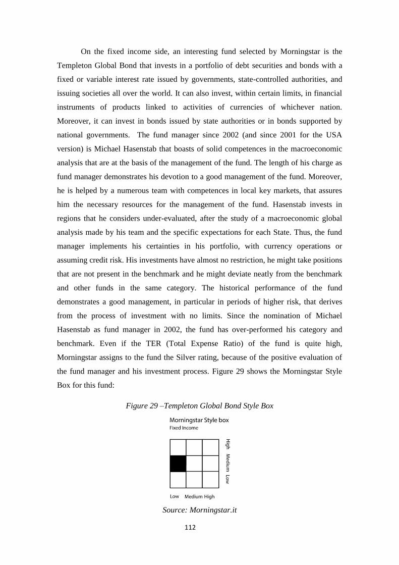
112
On the fixed income side, an interesting fund selected by Morningstar is the
Templeton Global Bond that invests in a portfolio of debt securities and bonds with a
fixed or variable interest rate issued by governments, state-controlled authorities, and
issuing societies all over the world. It can also invest, within certain limits, in financial
instruments of products linked to activities of currencies of whichever nation.
Moreover, it can invest in bonds issued by state authorities or in bonds supported by
national governments. The fund manager since 2002 (and since 2001 for the USA
version) is Michael Hasenstab that boasts of solid competences in the macroeconomic
analysis that are at the basis of the management of the fund. The length of his charge as
fund manager demonstrates his devotion to a good management of the fund. Moreover,
he is helped by a numerous team with competences in local key markets, that assures
him the necessary resources for the management of the fund. Hasenstab invests in
regions that he considers under-evaluated, after the study of a macroeconomic global
analysis made by his team and the specific expectations for each State. Thus, the fund
manager implements his certainties in his portfolio, with currency operations or
assuming credit risk. His investments have almost no restriction, he might take positions
that are not present in the benchmark and he might deviate neatly from the benchmark
and other funds in the same category. The historical performance of the fund
demonstrates a good management, in particular in periods of higher risk, that derives
from the process of investment with no limits. Since the nomination of Michael
Hasenstab as fund manager in 2002, the fund has over-performed his category and
benchmark. Even if the TER (Total Expense Ratio) of the fund is quite high,
Morningstar assigns to the fund the Silver rating, because of the positive evaluation of
the fund manager and his investment process. Figure 29 shows the Morningstar Style
Box for this fund:
Figure 29 –Templeton Global Bond Style Box
Source: Morningstar.it
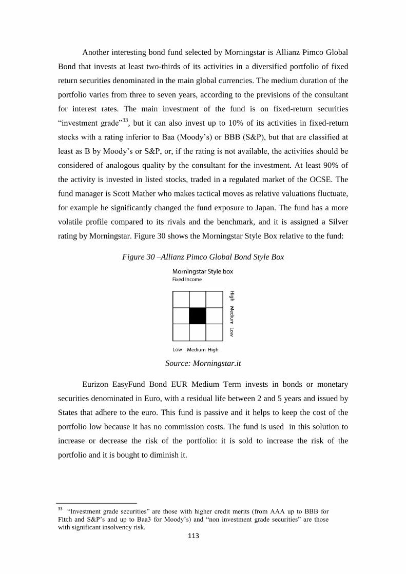
113
Another interesting bond fund selected by Morningstar is Allianz Pimco Global
Bond that invests at least two-thirds of its activities in a diversified portfolio of fixed
return securities denominated in the main global currencies. The medium duration of the
portfolio varies from three to seven years, according to the previsions of the consultant
for interest rates. The main investment of the fund is on fixed-return securities
―investment grade‖33
, but it can also invest up to 10% of its activities in fixed-return
stocks with a rating inferior to Baa (Moody‘s) or BBB (S&P), but that are classified at
least as B by Moody‘s or S&P, or, if the rating is not available, the activities should be
considered of analogous quality by the consultant for the investment. At least 90% of
the activity is invested in listed stocks, traded in a regulated market of the OCSE. The
fund manager is Scott Mather who makes tactical moves as relative valuations fluctuate,
for example he significantly changed the fund exposure to Japan. The fund has a more
volatile profile compared to its rivals and the benchmark, and it is assigned a Silver
rating by Morningstar. Figure 30 shows the Morningstar Style Box relative to the fund:
Figure 30 –Allianz Pimco Global Bond Style Box
Source: Morningstar.it
Eurizon EasyFund Bond EUR Medium Term invests in bonds or monetary
securities denominated in Euro, with a residual life between 2 and 5 years and issued by
States that adhere to the euro. This fund is passive and it helps to keep the cost of the
portfolio low because it has no commission costs. The fund is used in this solution to
increase or decrease the risk of the portfolio: it is sold to increase the risk of the
portfolio and it is bought to diminish it.
33
―Investment grade securities‖ are those with higher credit merits (from AAA up to BBB for
Fitch and S&P‘s and up to Baa3 for Moody‘s) and ―non investment grade securities‖ are those
with significant insolvency risk.
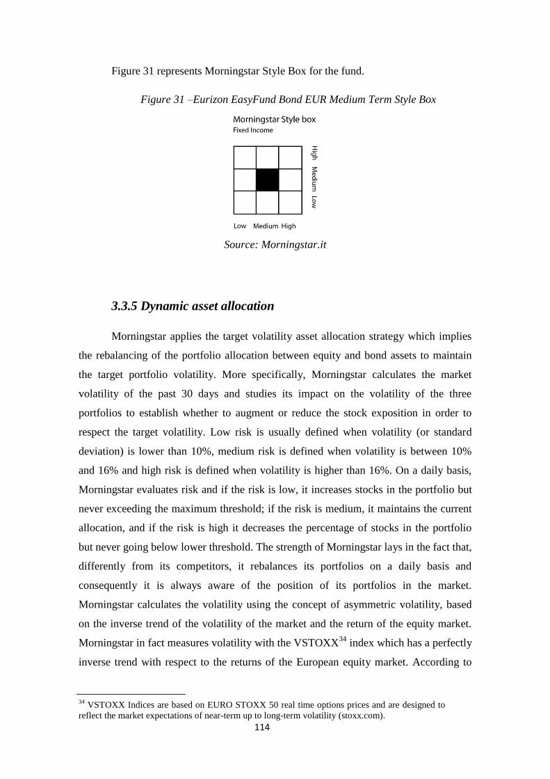
114
Figure 31 represents Morningstar Style Box for the fund.
Figure 31 –Eurizon EasyFund Bond EUR Medium Term Style Box
Source: Morningstar.it
3.3.5 Dynamic asset allocation
Morningstar applies the target volatility asset allocation strategy which implies
the rebalancing of the portfolio allocation between equity and bond assets to maintain
the target portfolio volatility. More specifically, Morningstar calculates the market
volatility of the past 30 days and studies its impact on the volatility of the three
portfolios to establish whether to augment or reduce the stock exposition in order to
respect the target volatility. Low risk is usually defined when volatility (or standard
deviation) is lower than 10%, medium risk is defined when volatility is between 10%
and 16% and high risk is defined when volatility is higher than 16%. On a daily basis,
Morningstar evaluates risk and if the risk is low, it increases stocks in the portfolio but
never exceeding the maximum threshold; if the risk is medium, it maintains the current
allocation, and if the risk is high it decreases the percentage of stocks in the portfolio
but never going below lower threshold. The strength of Morningstar lays in the fact that,
differently from its competitors, it rebalances its portfolios on a daily basis and
consequently it is always aware of the position of its portfolios in the market.
Morningstar calculates the volatility using the concept of asymmetric volatility, based
on the inverse trend of the volatility of the market and the return of the equity market.
Morningstar in fact measures volatility with the VSTOXX34
index which has a perfectly
inverse trend with respect to the returns of the European equity market. According to
34
VSTOXX Indices are based on EURO STOXX 50 real time options prices and are designed to
reflect the market expectations of near-term up to long-term volatility (stoxx.com).
115
this, when the VSTOXX index is high, it decreases the exposition to stocks in the
portfolios, when the volatility is low, it increases the percentage of stocks.
The peculiarity of this approach is that it considers every risk as an opportunity,
and so volatility is not only a parameter of evaluation of the risk of the portfolio, but it
is also a measure of market movements that hide big opportunities to catch. The
objective is that of avoiding losses that are avoidable and to benefit from eventual rises
in the market through flexibility. Dario Castagna, senior analyst at Morningstar
Associates and one of the four portfolio managers of the solution for Clerical Medical,
explains the strategy elaborated by the analysts of Morningstar Associates was born on
the intuition of doing an asset allocation based on the study of expected volatility, in the
light of the financial crisis of 2008, where neither the most defensive portfolios proved
to be immune from losses.
To have information over future volatility, Morningstar uses the following
model:
E(σ) = f ( , GARCH, VIX) (69)
Let us explain each element in more detailed: is the volatility of the last thirty
days using for simplicity the VSTOXX index. The GARCH (Generalized
Autoregressive Conditional Heteroskedasticity) is an econometric process to estimate
volatility in financial markets, providing a more real-world context than other models. It
is composed of three steps: the first one estimates a best-fitting autoregressive model,
the second one computes autocorrelations of the error terms and the last step tests for
significance. The VIX index is an index of expected future price volatility implied by
options contract prices. It is also called ―fear index‖ since its value increases when
investors are concerned about future volatility. In reality, high values of the index do not
necessarily indicate a fall in the market but they indicate that investors predict that
prices will go up or down substantially. The most important VIX index is the S&P 500
Vix Index that uses data from S&P 500 options contracts, calculating a weighted
average of the prices of various S&P 500 index options contracts. The VIX index tends
to spike when share prices plummet.
As already said, the expected volatility obtained with formula 3.1 is used to
rebalance the allocation in the portfolio (whether to increase, decrease or keep constant
the percentage of stocks in the portfolio). When changing the percentages of investment
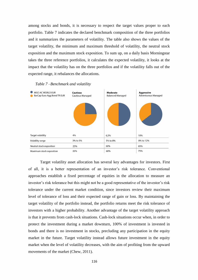
116
among stocks and bonds, it is necessary to respect the target values proper to each
portfolio. Table 7 indicates the declared benchmark composition of the three portfolios
and it summarizes the parameters of volatility. The table also shows the values of the
target volatility, the minimum and maximum threshold of volatility, the neutral stock
exposition and the maximum stock exposition. To sum up, on a daily basis Morningstar
takes the three reference portfolios, it calculates the expected volatility, it looks at the
impact that the volatility has on the three portfolios and if the volatility falls out of the
expected range, it rebalances the allocations.
Table 7 –Benchmark and volatility
Target volatility asset allocation has several key advantages for investors. First
of all, it is a better representation of an investor‘s risk tolerance. Conventional
approaches establish a fixed percentage of equities in the allocation to measure an
investor‘s risk tolerance but this might not be a good representative of the investor‘s risk
tolerance under the current market condition, since investors review their maximum
level of tolerance of loss and their expected range of gain or loss. By maintaining the
target volatility of the portfolio instead, the portfolio returns meet the risk tolerance of
investors with a higher probability. Another advantage of the target volatility approach
is that it prevents from cash-lock situations. Cash-lock situations occur when, in order to
protect the investment during a market downturn, 100% of investment is invested in
bonds and there is no investment in stocks, precluding any participation in the equity
market in the future. Target volatility instead allows future investment in the equity
market when the level of volatility decreases, with the aim of profiting from the upward
movements of the market (Chew, 2011).
117
In an article of Baselli for Morningstar (2014), Mr. Castagna explains this
concept making an example with a classic moderate portfolio of 60% of stocks and 40%
of bonds and a medium historical volatility of 11%, meaning that an investor with this
type of asset allocation expects a volatility of this level. This is a right consideration if
we consider the long run, but in the short run results might be very different: in October
2008, a sample moderate portfolio registered a volatility over 20%, while in 2006
volatility went down to 6-7%. This means that in some periods the risk is too high,
while in others it would be better to be more aggressive and thus to invest more in
stocks. According to Castagna, it is essential to put volatility under control: returns are
difficult to calculate, while volatility is much more predictable, because it moves in a
quite homogeneous way. The phenomenon of asymmetric volatility makes this even
easier: volatility is high when markets lose and it is low when markets rise. In the
example of the moderate portfolio, when the expected volatility is higher than 11% (the
risk is higher), the portfolio becomes more defensive, on the contrary, when a lower
volatility is predicted, the percentage of stocks is augmented. It is important to keep into
consideration that in order to use this approach it is necessary to have a wide and very
diversified portfolio. The great advantage of this approach, according to Castagna, is
that apart from the diversification condition, it can be applied to every portfolio and to
every type of investor.
3.3.6 Daily monitor and rebalancing
Monitoring and rebalancing are two constant activities in the management of the
three portfolios for Clerical Medical. And even if officially it is said that the strategic
asset allocation is reviewed on an annual basis, the monitoring of the funds takes place
on a monthly basis, and dynamic asset allocation is applied on a daily basis, in reality
the three activities are monitored and discussed on a daily basis (Castagna, 2013).
From the point of view of the strategic asset allocation, let us list some examples
of the changes in strategy made by Morningstar. An important decision has been the
introduction of the investment in Japan, by which Morningstar managers have been
attracted after the operation of quantitative easing of April 2013 and from which they
think they can catch a huge potential in the future. The introduction of this investment
took place only after the study of the correlation of Japan with the other asset classes in
118
the portfolios. Another strategic move has been the shift of investment in April 2013
from Euro Government bonds, that showed low interest rates, to Euro Corporate and
Global Bonds. Besides, on the European side, the investment focuses on high quality
European stocks, in particular in Germany, maintaining the overweight to the dollar that
helps to keep the value of the investment constant during financial markets downturns
(Castagna, 2013).
Morningstar selects the funds and keep them into the portfolio for a certain
period, since the portfolio managers think that the underlying funds should have the
time to realize their strategy. Also, portfolio managers do not expect each fund to ‗win‘
every time and every year in its category, but they expect that they have the possibility
to keep doing well in the long term. If this is not the case, the funds are substituted. A
practical example is the substitution of the fund Robeco with the fund Bluebay in April
2013. Other examples are the elimination of the fund American Small Cap and the
substitution of the AXA WF Global Inflation with Fidelity Fund Global Inflation
Linked Bond Fund. In the last example, the former has a duration of 12 years and the
last one has a duration of 5 years; Morningstar researchers in fact expect an increase of
interest rates and so they decided to reduce the duration of the portfolios. Following the
same principle, the fund Pioneer Funds Absolute return Bond, a fund that tries to
generate a performance independently from bond markets, was introduced in order to
reduce the risk of the portfolio on the fixed income side (Castagna, 2013).
3.4 Performance
In the recent years, many investors tended to focus their attention more on
mutual funds‘ historical performance than on the underlying portfolio characteristics.
We agree that investment returns are an important consideration, but it would probably
be better to start from looking at the portfolio fundamentals. We think that the
management by Morningstar provides a great added value and that top rated
performances are usually the consequence of the quality of the investment. In the
mutual fund industry, it is very important to consider all the characteristics of the funds
and to concentrate in the way they are managed. This is the approach followed by
Morningstar, also evidenced by its core business that concentrates on qualitative fund
analysis and on the provision of fundamental tools to allow the screening of mutual
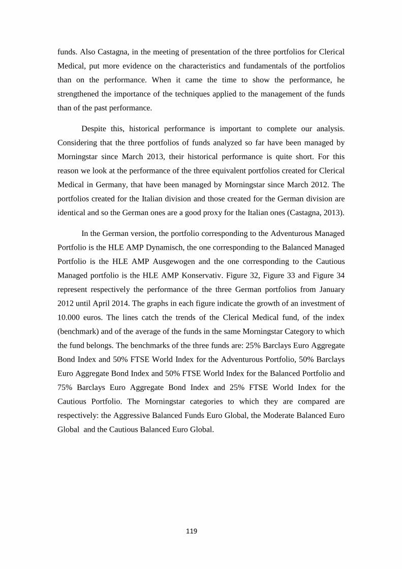
119
funds. Also Castagna, in the meeting of presentation of the three portfolios for Clerical
Medical, put more evidence on the characteristics and fundamentals of the portfolios
than on the performance. When it came the time to show the performance, he
strengthened the importance of the techniques applied to the management of the funds
than of the past performance.
Despite this, historical performance is important to complete our analysis.
Considering that the three portfolios of funds analyzed so far have been managed by
Morningstar since March 2013, their historical performance is quite short. For this
reason we look at the performance of the three equivalent portfolios created for Clerical
Medical in Germany, that have been managed by Morningstar since March 2012. The
portfolios created for the Italian division and those created for the German division are
identical and so the German ones are a good proxy for the Italian ones (Castagna, 2013).
In the German version, the portfolio corresponding to the Adventurous Managed
Portfolio is the HLE AMP Dynamisch, the one corresponding to the Balanced Managed
Portfolio is the HLE AMP Ausgewogen and the one corresponding to the Cautious
Managed portfolio is the HLE AMP Konservativ. Figure 32, Figure 33 and Figure 34
represent respectively the performance of the three German portfolios from January
2012 until April 2014. The graphs in each figure indicate the growth of an investment of
10.000 euros. The lines catch the trends of the Clerical Medical fund, of the index
(benchmark) and of the average of the funds in the same Morningstar Category to which
the fund belongs. The benchmarks of the three funds are: 25% Barclays Euro Aggregate
Bond Index and 50% FTSE World Index for the Adventurous Portfolio, 50% Barclays
Euro Aggregate Bond Index and 50% FTSE World Index for the Balanced Portfolio and
75% Barclays Euro Aggregate Bond Index and 25% FTSE World Index for the
Cautious Portfolio. The Morningstar categories to which they are compared are
respectively: the Aggressive Balanced Funds Euro Global, the Moderate Balanced Euro
Global and the Cautious Balanced Euro Global.
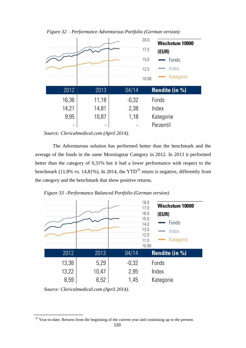
120
Figure 32 – Performance Adventurous Portfolio (German version)
Source: Clericalmedical.com (April 2014).
The Adventurous solution has performed better than the benchmark and the
average of the funds in the same Morningstar Category in 2012. In 2013 it performed
better than the category of 0,31% but it had a lower performance with respect to the
benchmark (11,8% vs. 14,81%). In 2014, the YTD35
return is negative, differently from
the category and the benchmark that show positive returns.
Figure 33 –Performance Balanced Portfolio (German version)
Source: Clericalmedical.com (April 2014).
35
Year-to-date. Returns from the beginning of the current year and continuing up to the present.
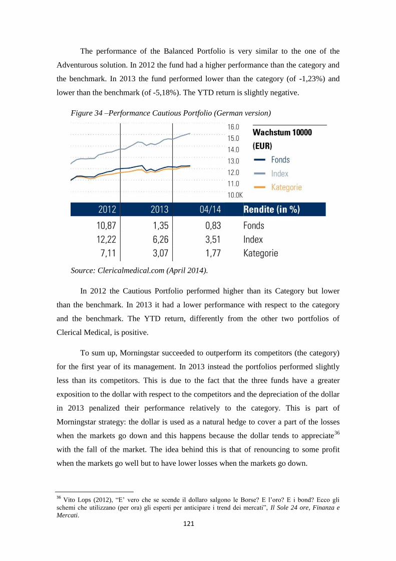
121
The performance of the Balanced Portfolio is very similar to the one of the
Adventurous solution. In 2012 the fund had a higher performance than the category and
the benchmark. In 2013 the fund performed lower than the category (of -1,23%) and
lower than the benchmark (of -5,18%). The YTD return is slightly negative.
Figure 34 –Performance Cautious Portfolio (German version)
Source: Clericalmedical.com (April 2014).
In 2012 the Cautious Portfolio performed higher than its Category but lower
than the benchmark. In 2013 it had a lower performance with respect to the category
and the benchmark. The YTD return, differently from the other two portfolios of
Clerical Medical, is positive.
To sum up, Morningstar succeeded to outperform its competitors (the category)
for the first year of its management. In 2013 instead the portfolios performed slightly
less than its competitors. This is due to the fact that the three funds have a greater
exposition to the dollar with respect to the competitors and the depreciation of the dollar
in 2013 penalized their performance relatively to the category. This is part of
Morningstar strategy: the dollar is used as a natural hedge to cover a part of the losses
when the markets go down and this happens because the dollar tends to appreciate36
with the fall of the market. The idea behind this is that of renouncing to some profit
when the markets go well but to have lower losses when the markets go down.
36
Vito Lops (2012), ―E‘ vero che se scende il dollaro salgono le Borse? E l‘oro? E i bond? Ecco gli
schemi che utilizzano (per ora) gli esperti per anticipare i trend dei mercati‖, Il Sole 24 ore, Finanza e
Mercati.

122
Considering that two years of performance do not say much, in the analysis
conducted in Chapter 4 we will use the fund BG Selection Global Risk Managed, a
fund managed by Morningstar for Generali Bank in Italy that was born under
Morningstar management in October 2009. The fund is a proxy of the Clerical Medical
Adventurous Portfolio.
123
Chapter 4
PORTFOLIO MANAGEMENT ANALYSIS
4.1 The CMIG Adventurous Managed Fund and the BG Selection
Global Risk Managed Fund
4.1.1 The proxy of the CMIG Adventurous Portfolio
As anticipated in the previous chapter , the three portfolios analyzed so far have
been managed by Morningstar since March 2013 and therefore they have a too recent
history to analyze. Even if we consider the three corresponding portfolios of the German
version that are managed by Morningstar since March 2012, the time period is not
significant enough to test Morningstar management. In fact, any analysis of both their
realized performance and effects of the management on the performance would be poor:
there is not much history that allows us to determine with a certain precision whether
the good or bad performance pursued by the fund is attributable to the management or it
is the consequence of coincidences, i.e. good or bad luck. To solve this problem, we
have chosen a good proxy of the Adventurous Managed Portfolio, represented by the
fund BG Selection Global Risk Managed AX, that has been managed by Morningstar
since October 2009 with the target volatility approach. When Mr. Castagna, one of the
portfolio managers, presented the solution to the partners of Clerical Medical in fact, he
referred to this fund to give an idea of how the portfolio has performed. Therefore, they
consider the two solutions pretty much similar. Indeed, the CMIG Adventurous
Managed fund and the BG Global Risk Managed fund are very similar in composition
and identical in the way they are managed. Let us provide a quick comparison and
description of the two funds to support our proxy.
The CMIG Adventurous Managed fund was created on the 23rd
of July 2004 and
Clerical Medical managed it until March 2013, when the management moved to
Morningstar. The current portfolio manager is Robin Johnson, a senior investment
consultant at Morningstar Investment Management Europe, who has a great experience
on investment consulting as a portfolio manager for Fund of Fund multi-asset strategies.
The objective of the fund is that of obtaining a growth of capital in the long term,
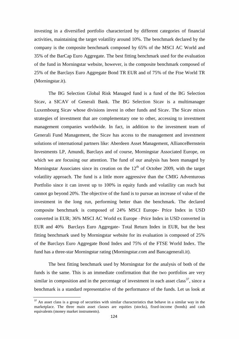
124
investing in a diversified portfolio characterized by different categories of financial
activities, maintaining the target volatility around 10%. The benchmark declared by the
company is the composite benchmark composed by 65% of the MSCI AC World and
35% of the BarCap Euro Aggregate. The best fitting benchmark used for the evaluation
of the fund in Morningstar website, however, is the composite benchmark composed of
25% of the Barclays Euro Aggregate Bond TR EUR and of 75% of the Ftse World TR
(Morningstar.it).
The BG Selection Global Risk Managed fund is a fund of the BG Selection
Sicav, a SICAV of Generali Bank. The BG Selection Sicav is a multimanager
Luxembourg Sicav whose divisions invest in other funds and Sicav. The Sicav mixes
strategies of investment that are complementary one to other, accessing to investment
management companies worldwide. In fact, in addition to the investment team of
Generali Fund Management, the Sicav has access to the management and investment
solutions of international partners like: Aberdeen Asset Management, AllianceBernstein
Investments LP, Amundi, Barclays and of course, Morningstar Associated Europe, on
which we are focusing our attention. The fund of our analysis has been managed by
Morningstar Associates since its creation on the 12th
of October 2009, with the target
volatility approach. The fund is a little more aggressive than the CMIG Adventurous
Portfolio since it can invest up to 100% in equity funds and volatility can reach but
cannot go beyond 20%. The objective of the fund is to pursue an increase of value of the
investment in the long run, performing better than the benchmark. The declared
composite benchmark is composed of 24% MSCI Europe- Price Index in USD
converted in EUR; 36% MSCI AC World ex Europe –Price Index in USD converted in
EUR and 40% Barclays Euro Aggregate- Total Return Index in EUR, but the best
fitting benchmark used by Morningstar website for its evaluation is composed of 25%
of the Barclays Euro Aggregate Bond Index and 75% of the FTSE World Index. The
fund has a three-star Morningstar rating (Morningstar.com and Bancagenerali.it).
The best fitting benchmark used by Morningstar for the analysis of both of the
funds is the same. This is an immediate confirmation that the two portfolios are very
similar in composition and in the percentage of investment in each asset class37
, since a
benchmark is a standard representative of the performance of the funds. Let us look at
37
An asset class is a group of securities with similar characteristics that behave in a similar way in the
marketplace. The three main asset classes are equities (stocks), fixed-income (bonds) and cash
equivalents (money market instruments).
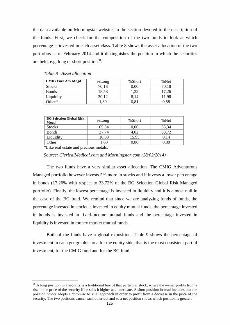
125
the data available on Morningstar website, in the section devoted to the description of
the funds. First, we check for the composition of the two funds to look at which
percentage is invested in each asset class. Table 8 shows the asset allocation of the two
portfolios as of February 2014 and it distinguishes the position in which the securities
are held, e.g. long or short position38
.
Table 8 –Asset allocation
CMIG Euro Adv Mngd %Long %Short %Net
Stocks 70,18 0,00 70,18
Bonds 18,58 1,32 17,26
Liquidity 20,12 8,14 11,98
Other* 1,39 0,81 0,58
BG Selection Global Risk
Mngd %Long %Short %Net
Stocks 65,34 0,00 65,34
Bonds 37,74 4,02 33,72
Liquidity 16,09 15,95 0,14
Other 1,60 0,80 0,80
*Like real estate and precious metals.
Source: ClericalMedical.com and Morningstar.com (28/02/2014).
The two funds have a very similar asset allocation. The CMIG Adventurous
Managed portfolio however invests 5% more in stocks and it invests a lower percentage
in bonds (17,26% with respect to 33,72% of the BG Selection Global Risk Managed
portfolio). Finally, the lowest percentage is invested in liquidity and it is almost null in
the case of the BG fund. We remind that since we are analyzing funds of funds, the
percentage invested in stocks is invested in equity mutual funds, the percentage invested
in bonds is invested in fixed-income mutual funds and the percentage invested in
liquidity is invested in money market mutual funds.
Both of the funds have a global exposition. Table 9 shows the percentage of
investment in each geographic area for the equity side, that is the most consistent part of
investment, for the CMIG fund and for the BG fund.
38
A long position in a security is a traditional buy of that particular stock, where the owner profits from a
rise in the price of the security if he sells it higher at a later date. A short position instead includes that the
position holder adopts a ―promise to sell‖ approach in order to profit from a decrease in the price of the
security. The two positions cancel each other out and so a net position shows which position is greater.
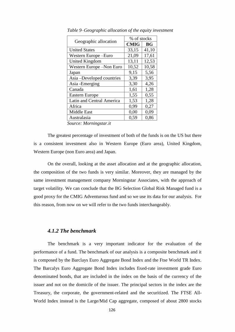
126
Table 9–Geographic allocation of the equity investment
Geographic allocation % of stocks
CMIG BG
United States 33,15 41,10
Western Europe –Euro 21,09 17,61
United Kingdom 13,11 12,53
Western Europe –Non Euro 10,52 10,58
Japan 9,15 5,56
Asia –Developed countries 3,39 3,95
Asia -Emerging 3,30 4,26
Canada 1,61 1,28
Eastern Europe 1,55 0,55
Latin and Central America 1,53 1,28
Africa 0,99 0,27
Middle East 0,00 0,09
Australasia 0,59 0,86
Source: Morningstar.it
The greatest percentage of investment of both of the funds is on the US but there
is a consistent investment also in Western Europe (Euro area), United Kingdom,
Western Europe (non Euro area) and Japan.
On the overall, looking at the asset allocation and at the geographic allocation,
the composition of the two funds is very similar. Moreover, they are managed by the
same investment management company Morningstar Associates, with the approach of
target volatility. We can conclude that the BG Selection Global Risk Managed fund is a
good proxy for the CMIG Adventurous fund and so we use its data for our analysis. For
this reason, from now on we will refer to the two funds interchangeably.
4.1.2 The benchmark
The benchmark is a very important indicator for the evaluation of the
performance of a fund. The benchmark of our analysis is a composite benchmark and it
is composed by the Barclays Euro Aggregate Bond Index and the Ftse World TR Index.
The Barcalys Euro Aggregate Bond Index includes fixed-rate investment grade Euro
denominated bonds, that are included in the index on the basis of the currency of the
issuer and not on the domicile of the issuer. The principal sectors in the index are the
Treasury, the corporate, the government-related and the securitized. The FTSE All-
World Index instead is the Large/Mid Cap aggregate, composed of about 2800 stocks
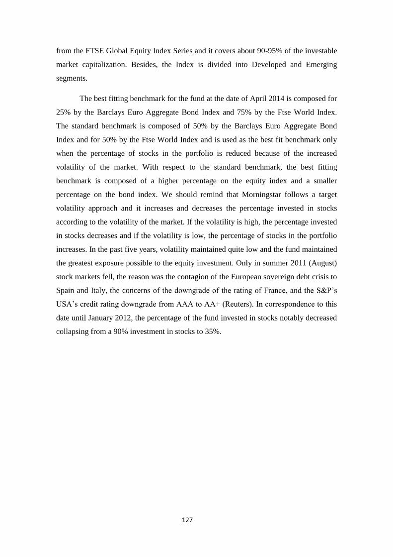
127
from the FTSE Global Equity Index Series and it covers about 90-95% of the investable
market capitalization. Besides, the Index is divided into Developed and Emerging
segments.
The best fitting benchmark for the fund at the date of April 2014 is composed for
25% by the Barclays Euro Aggregate Bond Index and 75% by the Ftse World Index.
The standard benchmark is composed of 50% by the Barclays Euro Aggregate Bond
Index and for 50% by the Ftse World Index and is used as the best fit benchmark only
when the percentage of stocks in the portfolio is reduced because of the increased
volatility of the market. With respect to the standard benchmark, the best fitting
benchmark is composed of a higher percentage on the equity index and a smaller
percentage on the bond index. We should remind that Morningstar follows a target
volatility approach and it increases and decreases the percentage invested in stocks
according to the volatility of the market. If the volatility is high, the percentage invested
in stocks decreases and if the volatility is low, the percentage of stocks in the portfolio
increases. In the past five years, volatility maintained quite low and the fund maintained
the greatest exposure possible to the equity investment. Only in summer 2011 (August)
stock markets fell, the reason was the contagion of the European sovereign debt crisis to
Spain and Italy, the concerns of the downgrade of the rating of France, and the S&P‘s
USA‘s credit rating downgrade from AAA to AA+ (Reuters). In correspondence to this
date until January 2012, the percentage of the fund invested in stocks notably decreased
collapsing from a 90% investment in stocks to 35%.
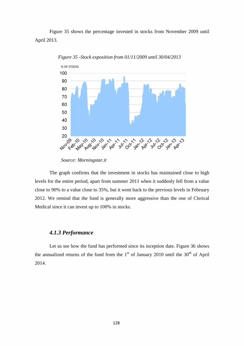
128
Figure 35 shows the percentage invested in stocks from November 2009 until
April 2013.
Figure 35 -Stock exposition from 01/11/2009 until 30/04/2013
Source: Morningstar.it
The graph confirms that the investment in stocks has maintained close to high
levels for the entire period, apart from summer 2011 when it suddenly fell from a value
close to 90% to a value close to 35%, but it went back to the previous levels in February
2012. We remind that the fund is generally more aggressive than the one of Clerical
Medical since it can invest up to 100% in stocks.
4.1.3 Performance
Let us see how the fund has performed since its inception date. Figure 36 shows
the annualized returns of the fund from the 1st of January 2010 until the 30
th of April
2014.
% OF STOCKS
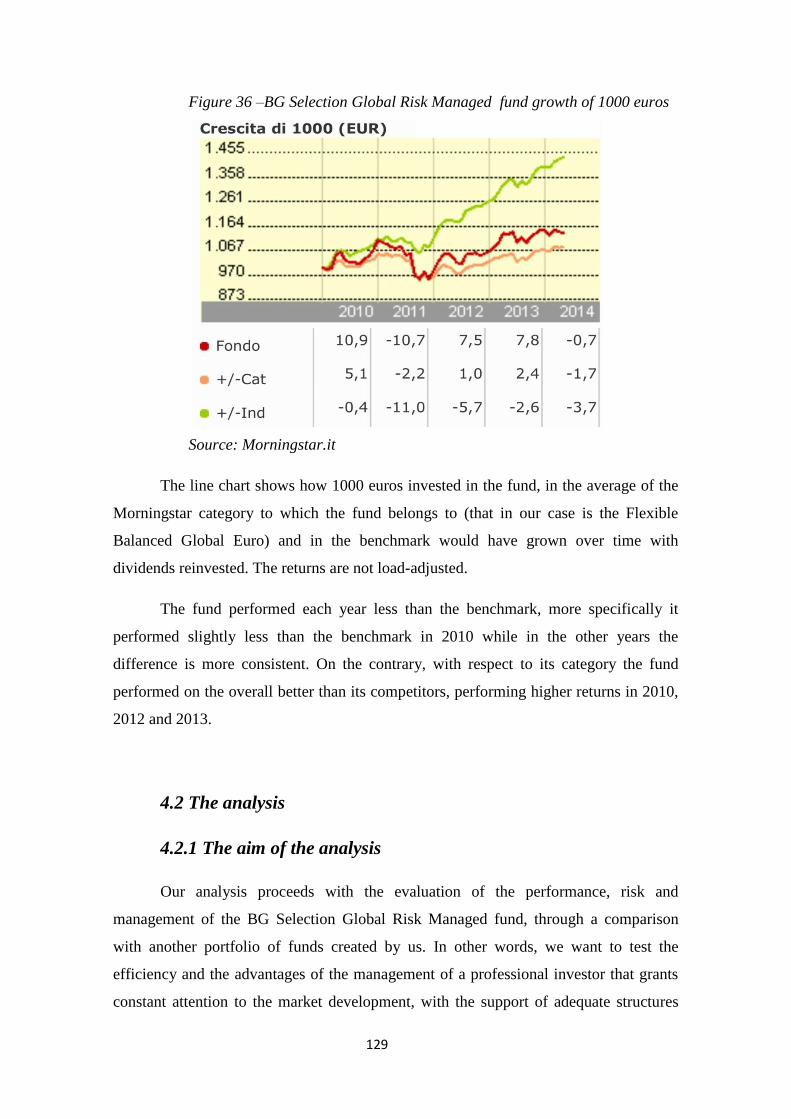
129
Figure 36 –BG Selection Global Risk Managed fund growth of 1000 euros
Source: Morningstar.it
The line chart shows how 1000 euros invested in the fund, in the average of the
Morningstar category to which the fund belongs to (that in our case is the Flexible
Balanced Global Euro) and in the benchmark would have grown over time with
dividends reinvested. The returns are not load-adjusted.
The fund performed each year less than the benchmark, more specifically it
performed slightly less than the benchmark in 2010 while in the other years the
difference is more consistent. On the contrary, with respect to its category the fund
performed on the overall better than its competitors, performing higher returns in 2010,
2012 and 2013.
4.2 The analysis
4.2.1 The aim of the analysis
Our analysis proceeds with the evaluation of the performance, risk and
management of the BG Selection Global Risk Managed fund, through a comparison
with another portfolio of funds created by us. In other words, we want to test the
efficiency and the advantages of the management of a professional investor that grants
constant attention to the market development, with the support of adequate structures
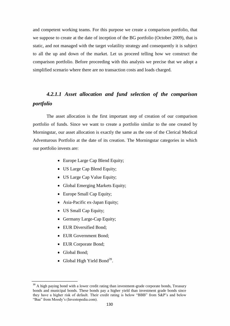
130
and competent working teams. For this purpose we create a comparison portfolio, that
we suppose to create at the date of inception of the BG portfolio (October 2009), that is
static, and not managed with the target volatility strategy and consequently it is subject
to all the up and down of the market. Let us proceed telling how we construct the
comparison portfolio. Before proceeding with this analysis we precise that we adopt a
simplified scenario where there are no transaction costs and loads charged.
4.2.1.1 Asset allocation and fund selection of the comparison
portfolio
The asset allocation is the first important step of creation of our comparison
portfolio of funds. Since we want to create a portfolio similar to the one created by
Morningstar, our asset allocation is exactly the same as the one of the Clerical Medical
Adventurous Portfolio at the date of its creation. The Morningstar categories in which
our portfolio invests are:
Europe Large Cap Blend Equity;
US Large Cap Blend Equity;
US Large Cap Value Equity;
Global Emerging Markets Equity;
Europe Small Cap Equity;
Asia-Pacific ex-Japan Equity;
US Small Cap Equity;
Germany Large-Cap Equity;
EUR Diversified Bond;
EUR Government Bond;
EUR Corporate Bond;
Global Bond;
Global High Yield Bond39
.
39
A high paying bond with a lower credit rating than investment-grade corporate bonds, Treasury
bonds and municipal bonds. These bonds pay a higher yield than investment grade bonds since
they have a higher risk of default. Their credit rating is below ―BBB‖ from S&P‘s and below
―Baa‖ from Moody‘s (Investopedia.com).

131
This asset allocation allows us to create a very diversified portfolio similar to the
one created by Morningstar. Our portfolio in fact has a diversified geographic
exposition and the funds differ for capitalization and style.
Once we have chosen the asset classes in which to invest, we select the funds to
include in the portfolio within each asset class in a way that, for each fund in the
Adventurous portfolio there is a corresponding fund in the comparison portfolio, chosen
from the same Morningstar category. Since we are supposing that the creation of our
portfolio dates back to October 2009, we choose funds whose inception date is prior to
that date of at least five years in, order to calculate variables like expected return,
variance (standard deviation) and correlation among assets with a certain precision.
Moreover, we select only funds denominated in euro and that are traded in Italy. Apart
from this, the choice of the funds is random, since we do not follow a precise strategy in
the selection of the funds. The main reason of this random selection is the impossibility
to go back to the date of creation of our portfolio without any biased data. The
Morningstar star rating, the Morningstar analyst rating and the Morningstar analysis
would be useful indicators to lead us in the choice of fund selection. However, we do
not have the instruments to know the rating and analysis of the funds at October 2009
and the data available today are contaminated by the events that have occurred so far.
Thus, it is impossible, for the instruments in our possession, to be stuck at October 2009
without any bias. Table 10 lists the 19 funds that we have selected for the comparison
portfolio. The first column indicates the ISIN code40
of each fund, the second column
indicates the name of the fund and the third column is the inception date of the fund,
that is the date in which the fund began its operations.
40
International Securities Identification Number, it is the code that uniquely identifies a security.
132
Table 10 –Funds selected for the comparison portfolio
ISIN Name Inception Date
LU0094541447 ABERDEEN GL-EUROPEAN EQU-A-2 01/02/1993
IT0000386588 ALLIANZ AZIONI EUROPA-L 11/03/1991
IT0001095469 ANIMA GEO EUROPA-A 02/06/1997
IT0001055075 AZIMUT AMERICA 23/10/1995
IE0003950965 BNY MELLON GL-EMRG MKT EQT V-A€ 02/08/2002
LU0133352731 CANDRIAM EQUITIES L-EMERG MKT-N 28/02/2002
LU0115016643 CAPITAL INT GLOBAL BOND-B EUR 03/04/1998
AT0000631916 ESPA BOND EURO TREND-A 02/02/2004
LU0149505165 INVESCO US STRUCT EQTY-E 28/06/2002
LU0117860493 JPMORGAN F-GERMANY EQUITY-D 13/10/2000
LU0052032793 KBC BONDS CAPITAL FUND-D 01/08/1973
GB0030939994 M&G ASIAN FUND -€-C-ACC 10/12/2001
LU0132602227 MORGAN STANLEY-EURO CORP BD-B 04/09/2001
LU0095343264 OYSTER EUROPEAN FIXED INCOME 04/03/1999
LU0131724808 PICTET-SMALL CAP EUR-I€ 01/03/1991
LU0190658715 PIONEER-GLB HI YLD-E ND € 18/06/2004
AT0000785340 RAIFFEISEN GLOBAL RENT-VT 26/05/1999
IE0002549826 RUSSELL US SML CAP EQ-C 31/03/1999
LU0106235889 SCHRODER INTL EURO BOND-C AC 17/01/2000
Our portfolio is composed by 8 fixed income funds and 11 equity funds, exactly
like the portfolio created by Morningstar. Table 11 indicates for each fund the general
asset class and the Morningstar asset class, that is more precise and gives an immediate
idea of definition of the geographic area of investment, the style and capitalization of
the fund.
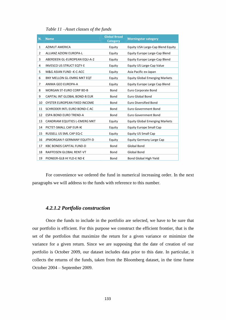
133
Table 11 –Asset classes of the funds
N. Name Global Broad
Category Morningstar category
1 AZIMUT AMERICA Equity Equity USA Large-Cap Blend Equity
2 ALLIANZ AZIONI EUROPA-L Equity Equity Europe Large-Cap Blend
3 ABERDEEN GL-EUROPEAN EQU-A-2 Equity Equity Europe Large-Cap Blend
4 INVESCO US STRUCT EQTY-E Equity Equity US Large-Cap Value
5 M&G ASIAN FUND -€-C-ACC Equity Asia Pacific ex-Japan
6 BNY MELLON GL-EMRG MKT EQT Equity Equity Global Emerging Markets
7 ANIMA GEO EUROPA-A Equity Equity Europe Large Cap Blend
8 MORGAN ST-EURO CORP BD-B Bond Euro Corporate Bond
9 CAPITAL INT GLOBAL BOND-B EUR Bond Euro Global Bond
10 OYSTER EUROPEAN FIXED INCOME Bond Euro Diversified Bond
11 SCHRODER INTL EURO BOND-C AC Bond Euro Government Bond
12 ESPA BOND EURO TREND-A Bond Euro Government Bond
13 CANDRIAM EQUITIES L-EMERG MKT Equity Equity Global Emerging Markets
14 PICTET-SMALL CAP EUR-I€ Equity Equity Europe Small Cap
15 RUSSELL US SML CAP EQ-C Equity Equity US Small Cap
16 JPMORGAN F-GERMANY EQUITY-D Equity Equity Germany Large Cap
17 KBC BONDS CAPITAL FUND-D Bond Global Bond
18 RAIFFEISEN GLOBAL RENT-VT Bond Global Bond
19 PIONEER-GLB HI YLD-E ND € Bond Bond Global High Yield
For convenience we ordered the fund in numerical increasing order. In the next
paragraphs we will address to the funds with reference to this number.
4.2.1.2 Portfolio construction
Once the funds to include in the portfolio are selected, we have to be sure that
our portfolio is efficient. For this purpose we construct the efficient frontier, that is the
set of the portfolios that maximize the return for a given variance or minimize the
variance for a given return. Since we are supposing that the date of creation of our
portfolio is October 2009, our dataset includes data prior to this date. In particular, it
collects the returns of the funds, taken from the Bloomberg dataset, in the time frame
October 2004 – September 2009.
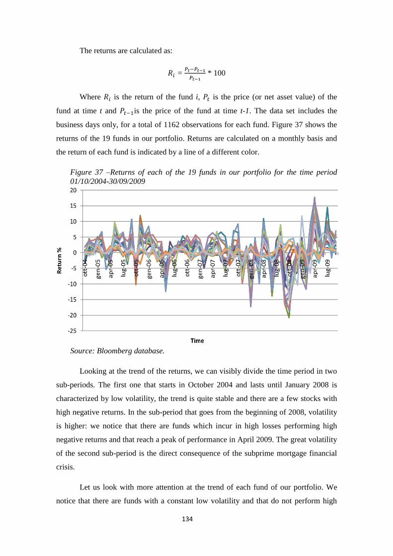
134
The returns are calculated as:
= * 100
Where is the return of the fund i, is the price (or net asset value) of the
fund at time t and is the price of the fund at time t-1. The data set includes the
business days only, for a total of 1162 observations for each fund. Figure 37 shows the
returns of the 19 funds in our portfolio. Returns are calculated on a monthly basis and
the return of each fund is indicated by a line of a different color.
Figure 37 –Returns of each of the 19 funds in our portfolio for the time period
01/10/2004-30/09/2009
Source: Bloomberg database.
Looking at the trend of the returns, we can visibly divide the time period in two
sub-periods. The first one that starts in October 2004 and lasts until January 2008 is
characterized by low volatility, the trend is quite stable and there are a few stocks with
high negative returns. In the sub-period that goes from the beginning of 2008, volatility
is higher: we notice that there are funds which incur in high losses performing high
negative returns and that reach a peak of performance in April 2009. The great volatility
of the second sub-period is the direct consequence of the subprime mortgage financial
crisis.
Let us look with more attention at the trend of each fund of our portfolio. We
notice that there are funds with a constant low volatility and that do not perform high
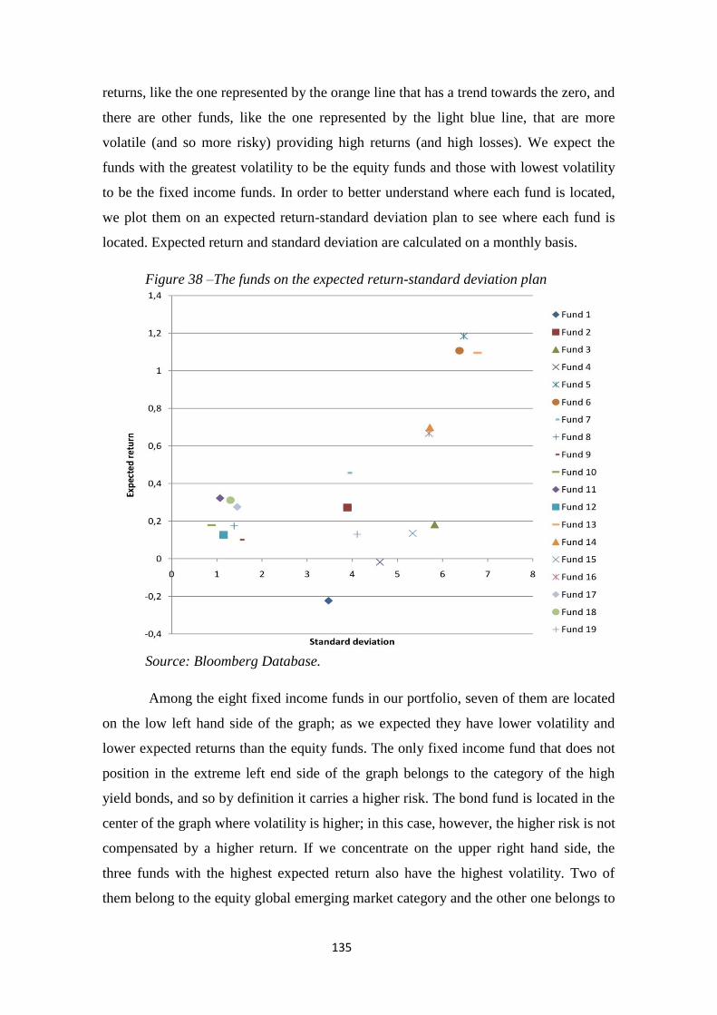
135
returns, like the one represented by the orange line that has a trend towards the zero, and
there are other funds, like the one represented by the light blue line, that are more
volatile (and so more risky) providing high returns (and high losses). We expect the
funds with the greatest volatility to be the equity funds and those with lowest volatility
to be the fixed income funds. In order to better understand where each fund is located,
we plot them on an expected return-standard deviation plan to see where each fund is
located. Expected return and standard deviation are calculated on a monthly basis.
Figure 38 –The funds on the expected return-standard deviation plan
Source: Bloomberg Database.
Among the eight fixed income funds in our portfolio, seven of them are located
on the low left hand side of the graph; as we expected they have lower volatility and
lower expected returns than the equity funds. The only fixed income fund that does not
position in the extreme left end side of the graph belongs to the category of the high
yield bonds, and so by definition it carries a higher risk. The bond fund is located in the
center of the graph where volatility is higher; in this case, however, the higher risk is not
compensated by a higher return. If we concentrate on the upper right hand side, the
three funds with the highest expected return also have the highest volatility. Two of
them belong to the equity global emerging market category and the other one belongs to

136
the Asia Pacific ex-Japan equity. The remaining funds concentrate in the middle of the
graph and two of them have negative expected returns.
4.2.1.3 The efficient frontier
We now want to find the set of the efficient combinations of the 19 funds. For
this purpose, we use the Solver in Excel that allows us to maximize or minimize an
objective function, modifying the values of some components of the objective function.
Let us explain in more detail the process of creation of the efficient frontier. As
already said, the data used here are the daily returns of the 19 mutual funds selected for
our portfolio, from the 1st of October 2004 until the 30
th of September 2009, for a total
of 1162 observations for each fund.
The first step is to compute the mean vector R and the variance-covariance matrix Ω.
The mean vector contains the expected return of each fund, and the variance-covariance
matrix consists of the variances of the funds along the main diagonal and the
covariances between each pair of funds in the other matrix positions. The R vector and
the Ω matrix41
of our problem (remember that the variance-covariance matrix is
symmetric with respect to the central diagonal) are respectively:
R:
-0,011 0,013 0,009 -0,001 0,056 0,053 0,022 0,008 0,005 0,009 0,015 0,006 0,052 0,033 0,006 0,031 0,013 0,015 0,006
Ω: 1,184 0,640 0,306 -0,002 0,378 0,112 0,676 -0,010 -0,018 -0,031 -0,031 0,004 0,920 0,566 1,696 0,513 -0,041 0,009 0,640 1,203 0,972 0,519 0,793 0,663 1,314 -0,035 -0,175 -0,054 -0,057 0,001 1,107 1,132 0,843 1,166 -0,168 -0,019 0,306 0,972 1,876 1,216 1,439 1,406 1,039 -0,022 -0,212 -0,054 -0,076 -0,068 1,388 1,132 0,328 1,468 -0,146 -0,091
-0,002 0,519 1,216 2,285 1,234 1,555 0,573 0,006 -0,040 -0,025 -0,050 -0,076 0,733 0,598 -0,049 0,856 -0,010 -0,060 0,378 0,793 1,439 1,234 2,217 1,793 0,861 0,001 -0,128 -0,046 -0,078 -0,073 1,746 1,004 0,495 1,129 -0,076 -0,075 0,112 0,663 1,406 1,555 1,793 1,980 0,720 0,013 -0,112 -0,042 -0,060 -0,092 1,407 0,868 0,224 1,018 -0,061 -0,127 0,676 1,314 1,039 0,573 0,861 0,720 1,391 -0,035 -0,191 -0,057 -0,059 0,001 1,183 1,200 0,869 1,255 -0,184 -0,019
-0,010 -0,035 -0,022 0,006 0,001 0,013 -0,035 0,068 0,037 0,020 0,025 0,008 -0,015 -0,023 -0,026 -0,039 0,033 0,002 -0,018 -0,175 -0,212 -0,040 -0,128 -0,112 -0,191 0,037 0,151 0,037 0,042 0,022 -0,166 -0,170 -0,004 -0,246 0,125 0,033 -0,031 -0,054 -0,054 -0,025 -0,046 -0,042 -0,057 0,020 0,037 0,028 0,024 0,010 -0,068 -0,048 -0,042 -0,064 0,040 0,011 -0,031 -0,057 -0,076 -0,050 -0,078 -0,060 -0,059 0,025 0,042 0,024 0,044 0,018 -0,076 -0,058 -0,048 -0,080 0,034 0,020 0,004 0,001 -0,068 -0,076 -0,073 -0,092 0,001 0,008 0,022 0,010 0,018 0,103 -0,052 -0,018 0,004 -0,029 0,010 0,057 0,920 1,107 1,388 0,733 1,746 1,407 1,183 -0,015 -0,166 -0,068 -0,076 -0,052 2,302 1,300 1,298 1,386 -0,120 -0,081 0,566 1,132 1,132 0,598 1,004 0,868 1,200 -0,023 -0,170 -0,048 -0,058 -0,018 1,300 1,301 0,787 1,233 -0,149 -0,035 1,696 0,843 0,328 -0,049 0,495 0,224 0,869 -0,026 -0,004 -0,042 -0,048 0,004 1,298 0,787 2,924 0,652 -0,020 0,000 0,513 1,166 1,468 0,856 1,129 1,018 1,255 -0,039 -0,246 -0,064 -0,080 -0,029 1,386 1,233 0,652 1,823 -0,188 -0,050
-0,041 -0,168 -0,146 -0,010 -0,076 -0,061 -0,184 0,033 0,125 0,040 0,034 0,010 -0,120 -0,149 -0,020 -0,188 0,138 0,013 0,009 -0,019 -0,091 -0,060 -0,075 -0,127 -0,019 0,002 0,033 0,011 0,020 0,057 -0,081 -0,035 0,000 -0,050 0,013 0,113 0,127 -0,105 -0,068 0,133 0,112 0,129 -0,132 0,031 0,143 0,014 0,008 0,003 0,105 -0,075 0,252 -0,147 0,149 0,003
41
The values in the vector and matrix are round to the third decimal place.
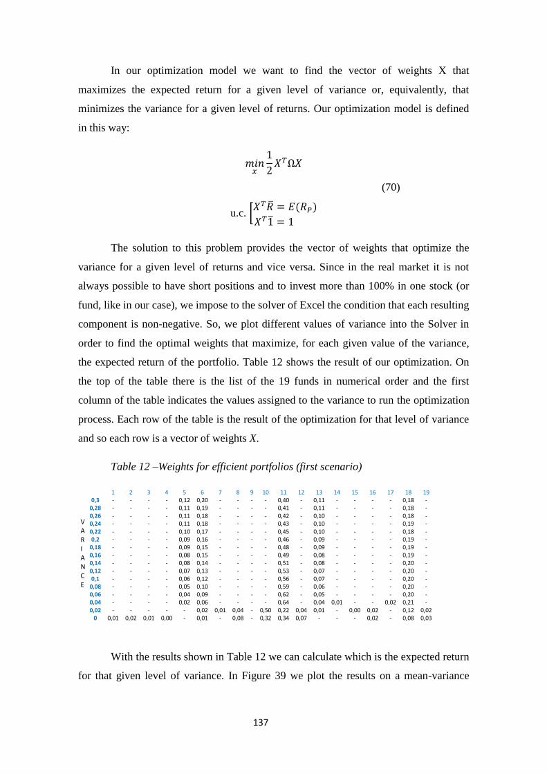
137
In our optimization model we want to find the vector of weights X that
maximizes the expected return for a given level of variance or, equivalently, that
minimizes the variance for a given level of returns. Our optimization model is defined
in this way:
(70)
u.c.
The solution to this problem provides the vector of weights that optimize the
variance for a given level of returns and vice versa. Since in the real market it is not
always possible to have short positions and to invest more than 100% in one stock (or
fund, like in our case), we impose to the solver of Excel the condition that each resulting
component is non-negative. So, we plot different values of variance into the Solver in
order to find the optimal weights that maximize, for each given value of the variance,
the expected return of the portfolio. Table 12 shows the result of our optimization. On
the top of the table there is the list of the 19 funds in numerical order and the first
column of the table indicates the values assigned to the variance to run the optimization
process. Each row of the table is the result of the optimization for that level of variance
and so each row is a vector of weights X.
Table 12 –Weights for efficient portfolios (first scenario)
1 2 3 4 5 6 7 8 9 10 11 12 13 14 15 16 17 18 19 0,3 - - - - 0,12 0,20 - - - - 0,40 - 0,11 - - - - 0,18 -
0,28 - - - - 0,11 0,19 - - - - 0,41 - 0,11 - - - - 0,18 - 0,26 - - - - 0,11 0,18 - - - - 0,42 - 0,10 - - - - 0,18 - 0,24 - - - - 0,11 0,18 - - - - 0,43 - 0,10 - - - - 0,19 - 0,22 - - - - 0,10 0,17 - - - - 0,45 - 0,10 - - - - 0,18 - 0,2 - - - - 0,09 0,16 - - - - 0,46 - 0,09 - - - - 0,19 -
0,18 - - - - 0,09 0,15 - - - - 0,48 - 0,09 - - - - 0,19 - 0,16 - - - - 0,08 0,15 - - - - 0,49 - 0,08 - - - - 0,19 - 0,14 - - - - 0,08 0,14 - - - - 0,51 - 0,08 - - - - 0,20 - 0,12 - - - - 0,07 0,13 - - - - 0,53 - 0,07 - - - - 0,20 - 0,1 - - - - 0,06 0,12 - - - - 0,56 - 0,07 - - - - 0,20 -
0,08 - - - - 0,05 0,10 - - - - 0,59 - 0,06 - - - - 0,20 - 0,06 - - - - 0,04 0,09 - - - - 0,62 - 0,05 - - - - 0,20 - 0,04 - - - - 0,02 0,06 - - - - 0,64 - 0,04 0,01 - - 0,02 0,21 - 0,02 - - - - - 0,02 0,01 0,04 - 0,50 0,22 0,04 0,01 - 0,00 0,02 - 0,12 0,02
0 0,01 0,02 0,01 0,00 - 0,01 - 0,08 - 0,32 0,34 0,07 - - - 0,02 - 0,08 0,03
With the results shown in Table 12 we can calculate which is the expected return
for that given level of variance. In Figure 39 we plot the results on a mean-variance
V A R I A N C E
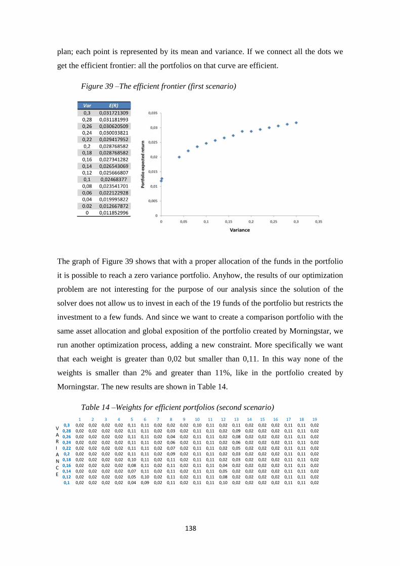
138
plan; each point is represented by its mean and variance. If we connect all the dots we
get the efficient frontier: all the portfolios on that curve are efficient.
Figure 39 –The efficient frontier (first scenario)
The graph of Figure 39 shows that with a proper allocation of the funds in the portfolio
it is possible to reach a zero variance portfolio. Anyhow, the results of our optimization
problem are not interesting for the purpose of our analysis since the solution of the
solver does not allow us to invest in each of the 19 funds of the portfolio but restricts the
investment to a few funds. And since we want to create a comparison portfolio with the
same asset allocation and global exposition of the portfolio created by Morningstar, we
run another optimization process, adding a new constraint. More specifically we want
that each weight is greater than 0,02 but smaller than 0,11. In this way none of the
weights is smaller than 2% and greater than 11%, like in the portfolio created by
Morningstar. The new results are shown in Table 14.
Table 14 –Weights for efficient portfolios (second scenario)
1 2 3 4 5 6 7 8 9 10 11 12 13 14 15 16 17 18 19 0,3 0,02 0,02 0,02 0,02 0,11 0,11 0,02 0,02 0,02 0,10 0,11 0,02 0,11 0,02 0,02 0,02 0,11 0,11 0,02
0,28 0,02 0,02 0,02 0,02 0,11 0,11 0,02 0,03 0,02 0,11 0,11 0,02 0,09 0,02 0,02 0,02 0,11 0,11 0,02 0,26 0,02 0,02 0,02 0,02 0,11 0,11 0,02 0,04 0,02 0,11 0,11 0,02 0,08 0,02 0,02 0,02 0,11 0,11 0,02 0,24 0,02 0,02 0,02 0,02 0,11 0,11 0,02 0,06 0,02 0,11 0,11 0,02 0,06 0,02 0,02 0,02 0,11 0,11 0,02 0,22 0,02 0,02 0,02 0,02 0,11 0,11 0,02 0,07 0,02 0,11 0,11 0,02 0,05 0,02 0,02 0,02 0,11 0,11 0,02 0,2 0,02 0,02 0,02 0,02 0,11 0,11 0,02 0,09 0,02 0,11 0,11 0,02 0,03 0,02 0,02 0,02 0,11 0,11 0,02
0,18 0,02 0,02 0,02 0,02 0,10 0,11 0,02 0,11 0,02 0,11 0,11 0,02 0,03 0,02 0,02 0,02 0,11 0,11 0,02 0,16 0,02 0,02 0,02 0,02 0,08 0,11 0,02 0,11 0,02 0,11 0,11 0,04 0,02 0,02 0,02 0,02 0,11 0,11 0,02 0,14 0,02 0,02 0,02 0,02 0,07 0,11 0,02 0,11 0,02 0,11 0,11 0,05 0,02 0,02 0,02 0,02 0,11 0,11 0,02 0,12 0,02 0,02 0,02 0,02 0,05 0,10 0,02 0,11 0,02 0,11 0,11 0,08 0,02 0,02 0,02 0,02 0,11 0,11 0,02 0,1 0,02 0,02 0,02 0,02 0,04 0,09 0,02 0,11 0,02 0,11 0,11 0,10 0,02 0,02 0,02 0,02 0,11 0,11 0,02
V A R I A N C E
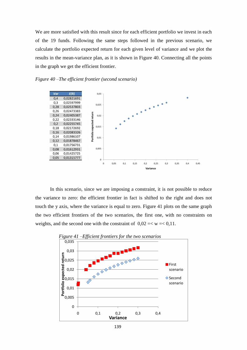
139
We are more satisfied with this result since for each efficient portfolio we invest in each
of the 19 funds. Following the same steps followed in the previous scenario, we
calculate the portfolio expected return for each given level of variance and we plot the
results in the mean-variance plan, as it is shown in Figure 40. Connecting all the points
in the graph we get the efficient frontier.
Figure 40 –The efficient frontier (second scenario)
In this scenario, since we are imposing a constraint, it is not possible to reduce
the variance to zero: the efficient frontier in fact is shifted to the right and does not
touch the y axis, where the variance is equal to zero. Figure 41 plots on the same graph
the two efficient frontiers of the two scenarios, the first one, with no constraints on
weights, and the second one with the constraint of 0,02 =< w =< 0,11.
Figure 41 –Efficient frontiers for the two scenarios
0
0,005
0,01
0,015
0,02
0,025
0,03
0,035
0 0,1 0,2 0,3 0,4
Po
rtfo
lio e
xpe
cte
d r
etu
rn
Variance
First scenario
Second scenario
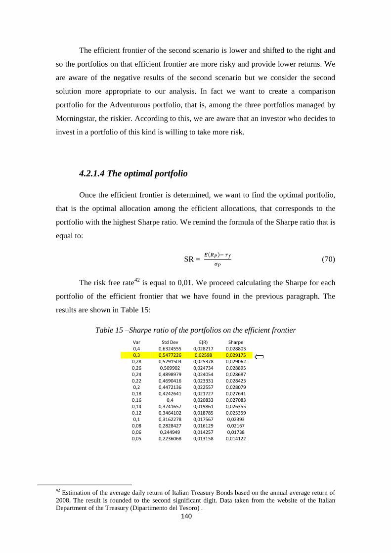
140
The efficient frontier of the second scenario is lower and shifted to the right and
so the portfolios on that efficient frontier are more risky and provide lower returns. We
are aware of the negative results of the second scenario but we consider the second
solution more appropriate to our analysis. In fact we want to create a comparison
portfolio for the Adventurous portfolio, that is, among the three portfolios managed by
Morningstar, the riskier. According to this, we are aware that an investor who decides to
invest in a portfolio of this kind is willing to take more risk.
4.2.1.4 The optimal portfolio
Once the efficient frontier is determined, we want to find the optimal portfolio,
that is the optimal allocation among the efficient allocations, that corresponds to the
portfolio with the highest Sharpe ratio. We remind the formula of the Sharpe ratio that is
equal to:
SR = (70)
The risk free rate42
is equal to 0,01. We proceed calculating the Sharpe for each
portfolio of the efficient frontier that we have found in the previous paragraph. The
results are shown in Table 15:
Table 15 –Sharpe ratio of the portfolios on the efficient frontier
Var Std Dev E(R) Sharpe 0,4 0,6324555 0,028217 0,028803 0,3 0,5477226 0,02598 0,029175
0,28 0,5291503 0,025378 0,029062 0,26 0,509902 0,024734 0,028895 0,24 0,4898979 0,024054 0,028687 0,22 0,4690416 0,023331 0,028423 0,2 0,4472136 0,022557 0,028079
0,18 0,4242641 0,021727 0,027641 0,16 0,4 0,020833 0,027083 0,14 0,3741657 0,019861 0,026355 0,12 0,3464102 0,018785 0,025359 0,1 0,3162278 0,017567 0,02393
0,08 0,2828427 0,016129 0,02167 0,06 0,244949 0,014257 0,01738 0,05 0,2236068 0,013158 0,014122
42
Estimation of the average daily return of Italian Treasury Bonds based on the annual average return of
2008. The result is rounded to the second significant digit. Data taken from the website of the Italian
Department of the Treasury (Dipartimento del Tesoro) .
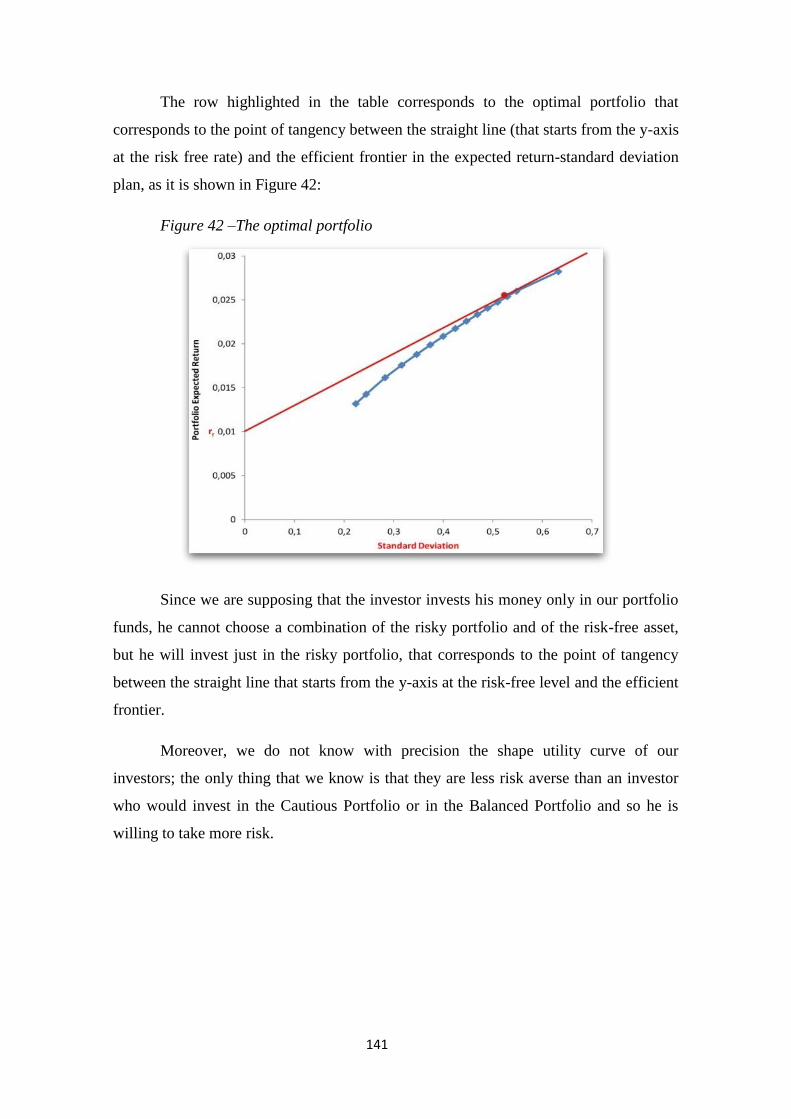
141
The row highlighted in the table corresponds to the optimal portfolio that
corresponds to the point of tangency between the straight line (that starts from the y-axis
at the risk free rate) and the efficient frontier in the expected return-standard deviation
plan, as it is shown in Figure 42:
Figure 42 –The optimal portfolio
Since we are supposing that the investor invests his money only in our portfolio
funds, he cannot choose a combination of the risky portfolio and of the risk-free asset,
but he will invest just in the risky portfolio, that corresponds to the point of tangency
between the straight line that starts from the y-axis at the risk-free level and the efficient
frontier.
Moreover, we do not know with precision the shape utility curve of our
investors; the only thing that we know is that they are less risk averse than an investor
who would invest in the Cautious Portfolio or in the Balanced Portfolio and so he is
willing to take more risk.
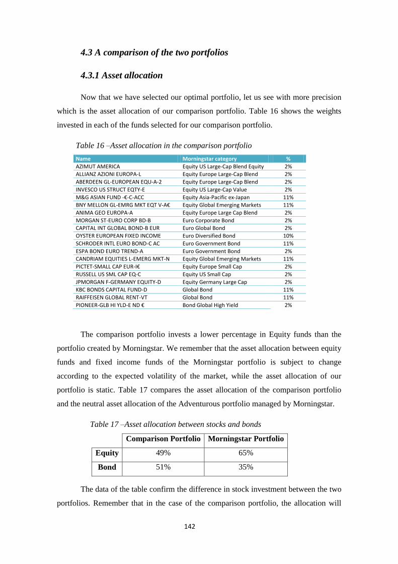
142
4.3 A comparison of the two portfolios
4.3.1 Asset allocation
Now that we have selected our optimal portfolio, let us see with more precision
which is the asset allocation of our comparison portfolio. Table 16 shows the weights
invested in each of the funds selected for our comparison portfolio.
Table 16 –Asset allocation in the comparison portfolio
Name Morningstar category %
AZIMUT AMERICA Equity US Large-Cap Blend Equity 2%
ALLIANZ AZIONI EUROPA-L Equity Europe Large-Cap Blend 2%
ABERDEEN GL-EUROPEAN EQU-A-2 Equity Europe Large-Cap Blend 2%
INVESCO US STRUCT EQTY-E Equity US Large-Cap Value 2%
M&G ASIAN FUND -€-C-ACC Equity Asia-Pacific ex-Japan 11%
BNY MELLON GL-EMRG MKT EQT V-A€ Equity Global Emerging Markets 11%
ANIMA GEO EUROPA-A Equity Europe Large Cap Blend 2%
MORGAN ST-EURO CORP BD-B Euro Corporate Bond 2%
CAPITAL INT GLOBAL BOND-B EUR Euro Global Bond 2%
OYSTER EUROPEAN FIXED INCOME Euro Diversified Bond 10%
SCHRODER INTL EURO BOND-C AC Euro Government Bond 11%
ESPA BOND EURO TREND-A Euro Government Bond 2%
CANDRIAM EQUITIES L-EMERG MKT-N Equity Global Emerging Markets 11%
PICTET-SMALL CAP EUR-I€ Equity Europe Small Cap 2%
RUSSELL US SML CAP EQ-C Equity US Small Cap 2%
JPMORGAN F-GERMANY EQUITY-D Equity Germany Large Cap 2%
KBC BONDS CAPITAL FUND-D Global Bond 11%
RAIFFEISEN GLOBAL RENT-VT Global Bond 11%
PIONEER-GLB HI YLD-E ND € Bond Global High Yield 2%
The comparison portfolio invests a lower percentage in Equity funds than the
portfolio created by Morningstar. We remember that the asset allocation between equity
funds and fixed income funds of the Morningstar portfolio is subject to change
according to the expected volatility of the market, while the asset allocation of our
portfolio is static. Table 17 compares the asset allocation of the comparison portfolio
and the neutral asset allocation of the Adventurous portfolio managed by Morningstar.
Table 17 –Asset allocation between stocks and bonds
Comparison Portfolio Morningstar Portfolio
Equity 49% 65%
Bond 51% 35%
The data of the table confirm the difference in stock investment between the two
portfolios. Remember that in the case of the comparison portfolio, the allocation will
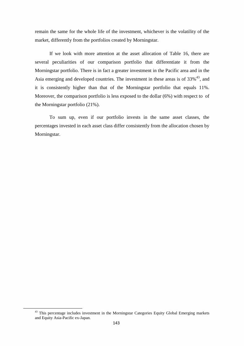
143
remain the same for the whole life of the investment, whichever is the volatility of the
market, differently from the portfolios created by Morningstar.
If we look with more attention at the asset allocation of Table 16, there are
several peculiarities of our comparison portfolio that differentiate it from the
Morningstar portfolio. There is in fact a greater investment in the Pacific area and in the
Asia emerging and developed countries. The investment in these areas is of 33%43
, and
it is consistently higher than that of the Morningstar portfolio that equals 11%.
Moreover, the comparison portfolio is less exposed to the dollar (6%) with respect to of
the Morningstar portfolio (21%).
To sum up, even if our portfolio invests in the same asset classes, the
percentages invested in each asset class differ consistently from the allocation chosen by
Morningstar.
43
This percentage includes investment in the Morningstar Categories Equity Global Emerging markets
and Equity Asia-Pacific ex-Japan.
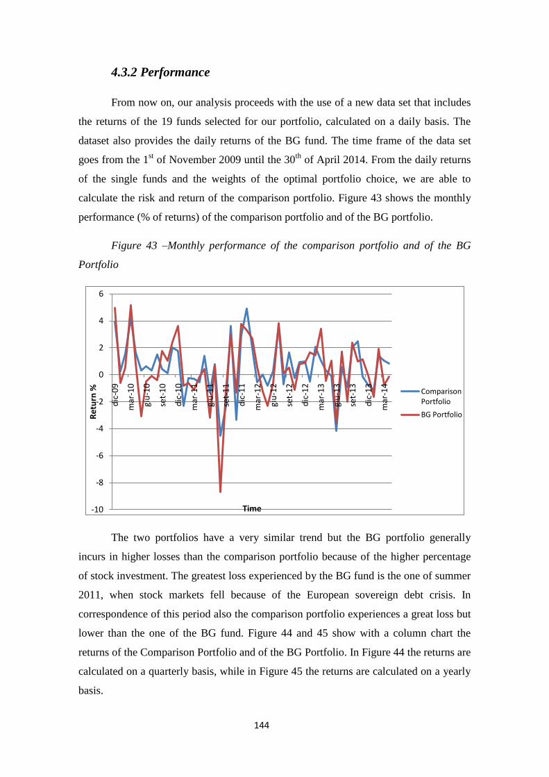
144
4.3.2 Performance
From now on, our analysis proceeds with the use of a new data set that includes
the returns of the 19 funds selected for our portfolio, calculated on a daily basis. The
dataset also provides the daily returns of the BG fund. The time frame of the data set
goes from the 1st of November 2009 until the 30
th of April 2014. From the daily returns
of the single funds and the weights of the optimal portfolio choice, we are able to
calculate the risk and return of the comparison portfolio. Figure 43 shows the monthly
performance (% of returns) of the comparison portfolio and of the BG portfolio.
Figure 43 –Monthly performance of the comparison portfolio and of the BG
Portfolio
The two portfolios have a very similar trend but the BG portfolio generally
incurs in higher losses than the comparison portfolio because of the higher percentage
of stock investment. The greatest loss experienced by the BG fund is the one of summer
2011, when stock markets fell because of the European sovereign debt crisis. In
correspondence of this period also the comparison portfolio experiences a great loss but
lower than the one of the BG fund. Figure 44 and 45 show with a column chart the
returns of the Comparison Portfolio and of the BG Portfolio. In Figure 44 the returns are
calculated on a quarterly basis, while in Figure 45 the returns are calculated on a yearly
basis.
-10
-8
-6
-4
-2
0
2
4
6
dic
-09
mar
-10
giu
-10
set-
10
dic
-10
mar
-11
giu
-11
set-
11
dic
-11
mar
-12
giu
-12
set-
12
dic
-12
mar
-13
giu
-13
set-
13
dic
-13
mar
-14
Re
turn
%
Time
Comparison Portfolio
BG Portfolio
145
Figure 44 –Portfolios returns on a quarterly basis
Our analysis includes 17 quarters. There are only two quarters (the 2nd
quarter
of 2010 and the 1st quarter of 2014) where the two funds have an opposite trend, in
particular the BG fund experiences negative returns and the comparison portfolio
performs positive returns. In all the other quarters the funds move in the same direction.
Table 18 indicates the number of positive and negative quarters for the two funds.
Table 18 –Positive and negative quarters
Comparison Portfolio BG Portfolio
Positive Quarters 12 10
Negative Quarters 5 7
Worst Quarter -6,106 -9,216
To sum up, there is a majority of positive quarters than negative quarters for
both the funds. As anticipated, the comparison portfolio has two quarters of positive
returns more than the BG portfolio, this is mainly caused by the greatest exposition to
risk of the BG portfolio. The table also indicates the worst return performed by each of
the funds (that in both cases corresponds to the third quarter of 2011). The loss of the
BG fund is greater, so even if in correspondence of this period Morningstar consistently
decreased the level of stocks in its portfolio, this operation did not totally control the
losses. This is probably due to the fact that this loss is caused by a fall of the entire
-12
-10
-8
-6
-4
-2
0
2
4
6
8
1st
Q. 2
01
0
2n
d Q
. 20
10
3rd
Q. 2
01
0
4th
Q. 2
01
0
1st
Q. 2
01
1
2n
d Q
. 20
11
3rd
Q. 2
01
1
4th
Q. 2
01
1
1st
Q. 2
01
2
2n
d Q
. 20
12
3rd
Q. 2
01
2
4th
Q. 2
01
2
1st
Q. 2
01
3
2n
d Q
. 20
13
3rd
Q. 2
01
3
4th
Q. 2
01
3
1st
Q. 2
01
4
Comparison Portfolio
BG Portfolio
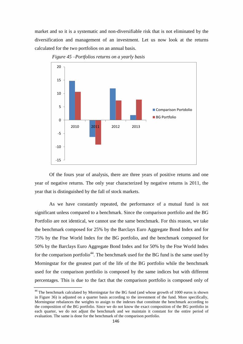
146
market and so it is a systematic and non-diversifiable risk that is not eliminated by the
diversification and management of an investment. Let us now look at the returns
calculated for the two portfolios on an annual basis.
Figure 45 –Portfolios returns on a yearly basis
Of the fours year of analysis, there are three years of positive returns and one
year of negative returns. The only year characterized by negative returns is 2011, the
year that is distinguished by the fall of stock markets.
As we have constantly repeated, the performance of a mutual fund is not
significant unless compared to a benchmark. Since the comparison portfolio and the BG
Portfolio are not identical, we cannot use the same benchmark. For this reason, we take
the benchmark composed for 25% by the Barclays Euro Aggregate Bond Index and for
75% by the Ftse World Index for the BG portfolio, and the benchmark composed for
50% by the Barclays Euro Aggregate Bond Index and for 50% by the Ftse World Index
for the comparison portfolio44
. The benchmark used for the BG fund is the same used by
Morningstar for the greatest part of the life of the BG portfolio while the benchmark
used for the comparison portfolio is composed by the same indices but with different
percentages. This is due to the fact that the comparison portfolio is composed only of
44
The benchmark calculated by Morningstar for the BG fund (and whose growth of 1000 euros is shown
in Figure 36) is adjusted on a quarter basis according to the investment of the fund. More specifically,
Morningstar rebalances the weights to assign to the indexes that constitute the benchmark according to
the composition of the BG portfolio. Since we do not know the exact composition of the BG portfolio in
each quarter, we do not adjust the benchmark and we maintain it constant for the entire period of
evaluation. The same is done for the benchmark of the comparison portfolio.
-15
-10
-5
0
5
10
15
20
2010 2011 2012 2013
Comparison Portdolio
BG Portfolio
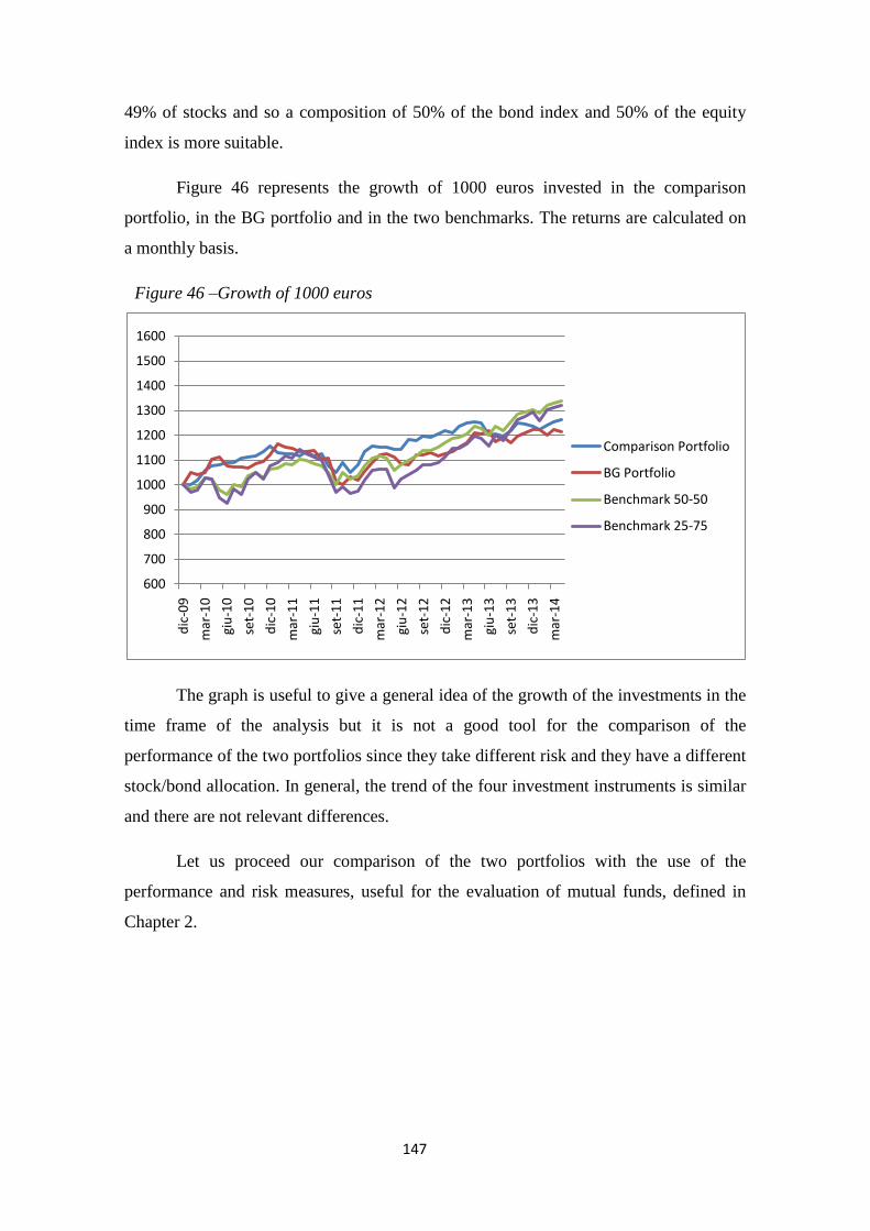
147
49% of stocks and so a composition of 50% of the bond index and 50% of the equity
index is more suitable.
Figure 46 represents the growth of 1000 euros invested in the comparison
portfolio, in the BG portfolio and in the two benchmarks. The returns are calculated on
a monthly basis.
Figure 46 –Growth of 1000 euros
The graph is useful to give a general idea of the growth of the investments in the
time frame of the analysis but it is not a good tool for the comparison of the
performance of the two portfolios since they take different risk and they have a different
stock/bond allocation. In general, the trend of the four investment instruments is similar
and there are not relevant differences.
Let us proceed our comparison of the two portfolios with the use of the
performance and risk measures, useful for the evaluation of mutual funds, defined in
Chapter 2.
600
700
800
900
1000
1100
1200
1300
1400
1500
1600
dic
-09
mar
-10
giu
-10
set-
10
dic
-10
mar
-11
giu
-11
set-
11
dic
-11
mar
-12
giu
-12
set-
12
dic
-12
mar
-13
giu
-13
set-
13
dic
-13
mar
-14
Comparison Portfolio
BG Portfolio
Benchmark 50-50
Benchmark 25-75
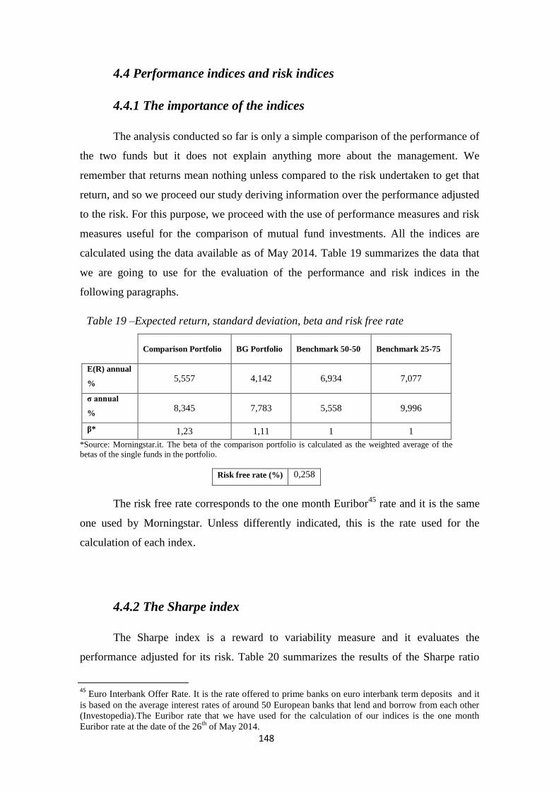
148
4.4 Performance indices and risk indices
4.4.1 The importance of the indices
The analysis conducted so far is only a simple comparison of the performance of
the two funds but it does not explain anything more about the management. We
remember that returns mean nothing unless compared to the risk undertaken to get that
return, and so we proceed our study deriving information over the performance adjusted
to the risk. For this purpose, we proceed with the use of performance measures and risk
measures useful for the comparison of mutual fund investments. All the indices are
calculated using the data available as of May 2014. Table 19 summarizes the data that
we are going to use for the evaluation of the performance and risk indices in the
following paragraphs.
Table 19 –Expected return, standard deviation, beta and risk free rate
Comparison Portfolio BG Portfolio Benchmark 50-50 Benchmark 25-75
E(R) annual
% 5,557 4,142 6,934 7,077
σ annual
% 8,345 7,783 5,558 9,996
β* 1,23 1,11 1 1
*Source: Morningstar.it. The beta of the comparison portfolio is calculated as the weighted average of the
betas of the single funds in the portfolio.
Risk free rate (%) 0,258
The risk free rate corresponds to the one month Euribor45
rate and it is the same
one used by Morningstar. Unless differently indicated, this is the rate used for the
calculation of each index.
4.4.2 The Sharpe index
The Sharpe index is a reward to variability measure and it evaluates the
performance adjusted for its risk. Table 20 summarizes the results of the Sharpe ratio
45
Euro Interbank Offer Rate. It is the rate offered to prime banks on euro interbank term deposits and it
is based on the average interest rates of around 50 European banks that lend and borrow from each other
(Investopedia).The Euribor rate that we have used for the calculation of our indices is the one month
Euribor rate at the date of the 26th
of May 2014.
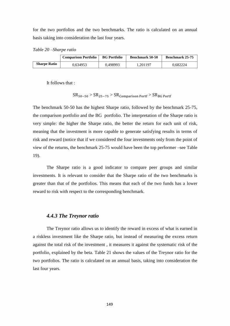
149
for the two portfolios and the two benchmarks. The ratio is calculated on an annual
basis taking into consideration the last four years.
Table 20 –Sharpe ratio
Comparison Portfolio BG Portfolio Benchmark 50-50 Benchmark 25-75
Sharpe Ratio 0,634953 0,498993 1,201197 0,682224
It follows that :
> > >
The benchmark 50-50 has the highest Sharpe ratio, followed by the benchmark 25-75,
the comparison portfolio and the BG portfolio. The interpretation of the Sharpe ratio is
very simple: the higher the Sharpe ratio, the better the return for each unit of risk,
meaning that the investment is more capable to generate satisfying results in terms of
risk and reward (notice that if we considered the four investments only from the point of
view of the returns, the benchmark 25-75 would have been the top performer –see Table
19).
The Sharpe ratio is a good indicator to compare peer groups and similar
investments. It is relevant to consider that the Sharpe ratio of the two benchmarks is
greater than that of the portfolios. This means that each of the two funds has a lower
reward to risk with respect to the corresponding benchmark.
4.4.3 The Treynor ratio
The Treynor ratio allows us to identify the reward in excess of what is earned in
a riskless investment like the Sharpe ratio, but instead of measuring the excess return
against the total risk of the investment , it measures it against the systematic risk of the
portfolio, explained by the beta. Table 21 shows the values of the Treynor ratio for the
two portfolios. The ratio is calculated on an annual basis, taking into consideration the
last four years.
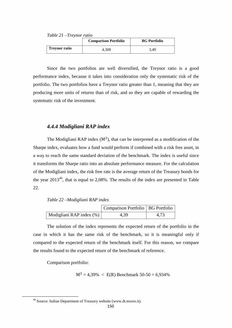
150
Table 21 –Treynor ratio
Comparison Portfolio BG Portfolio
Treynor ratio
annual
4,308 3,49
Since the two portfolios are well diversified, the Treynor ratio is a good
performance index, because it takes into consideration only the systematic risk of the
portfolio. The two portfolios have a Treynor ratio greater than 1, meaning that they are
producing more units of returns than of risk, and so they are capable of rewarding the
systematic risk of the investment.
4.4.4 Modigliani RAP index
The Modigliani RAP index ( ), that can be interpreted as a modification of the
Sharpe index, evaluates how a fund would perform if combined with a risk free asset, in
a way to reach the same standard deviation of the benchmark. The index is useful since
it transforms the Sharpe ratio into an absolute performance measure. For the calculation
of the Modigliani index, the risk free rate is the average return of the Treasury bonds for
the year 201346
, that is equal to 2,08%. The results of the index are presented in Table
22.
Table 22 –Modigliani RAP index
Comparison Portfolio BG Portfolio
Modigliani RAP index (%) 4,39 4,73
The solution of the index represents the expected return of the portfolio in the
case in which it has the same risk of the benchmark, so it is meaningful only if
compared to the expected return of the benchmark itself. For this reason, we compare
the results found to the expected return of the benchmark of reference.
Comparison portfolio:
= 4,39% < E(R) Benchmark 50-50 = 6,934%
46
Source: Italian Department of Treasury website (www.dt.tesoro.it).
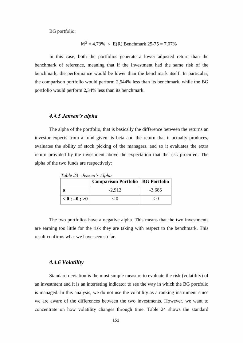
151
BG portfolio:
= 4,73% < E(R) Benchmark 25-75 = 7,07%
In this case, both the portfolios generate a lower adjusted return than the
benchmark of reference, meaning that if the investment had the same risk of the
benchmark, the performance would be lower than the benchmark itself. In particular,
the comparison portfolio would perform 2,544% less than its benchmark, while the BG
portfolio would perform 2,34% less than its benchmark.
4.4.5 Jensen’s alpha
The alpha of the portfolio, that is basically the difference between the returns an
investor expects from a fund given its beta and the return that it actually produces,
evaluates the ability of stock picking of the managers, and so it evaluates the extra
return provided by the investment above the expectation that the risk procured. The
alpha of the two funds are respectively:
Table 23 –Jensen’s Alpha
Comparison Portfolio BG Portfolio
α -2,912 -3,685
< 0 ; =0 ; >0 < 0 < 0
The two portfolios have a negative alpha. This means that the two investments
are earning too little for the risk they are taking with respect to the benchmark. This
result confirms what we have seen so far.
4.4.6 Volatility
Standard deviation is the most simple measure to evaluate the risk (volatility) of
an investment and it is an interesting indicator to see the way in which the BG portfolio
is managed. In this analysis, we do not use the volatility as a ranking instrument since
we are aware of the differences between the two investments. However, we want to
concentrate on how volatility changes through time. Table 24 shows the standard
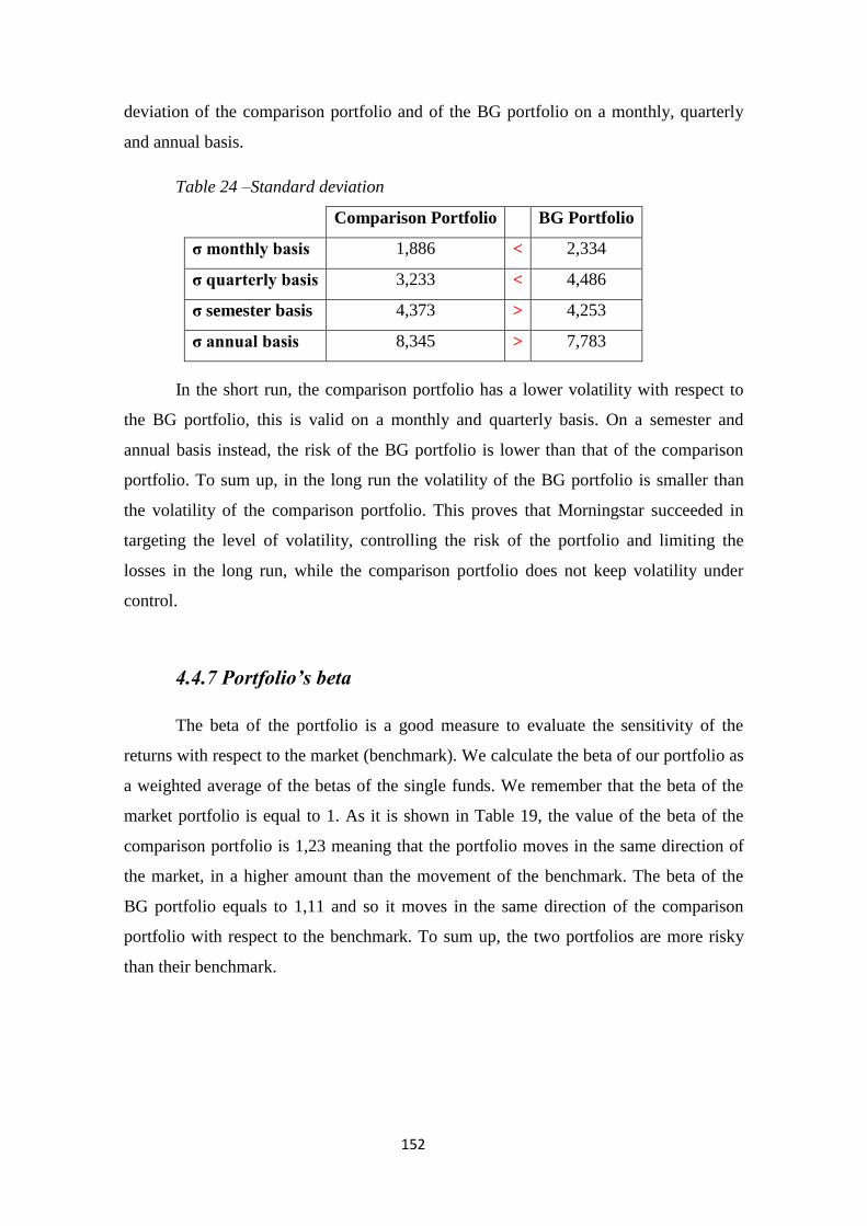
152
deviation of the comparison portfolio and of the BG portfolio on a monthly, quarterly
and annual basis.
Table 24 –Standard deviation
Comparison Portfolio BG Portfolio
σ monthly basis 1,886 < 2,334
σ quarterly basis 3,233 < 4,486
σ semester basis 4,373 > 4,253
σ annual basis 8,345 > 7,783
In the short run, the comparison portfolio has a lower volatility with respect to
the BG portfolio, this is valid on a monthly and quarterly basis. On a semester and
annual basis instead, the risk of the BG portfolio is lower than that of the comparison
portfolio. To sum up, in the long run the volatility of the BG portfolio is smaller than
the volatility of the comparison portfolio. This proves that Morningstar succeeded in
targeting the level of volatility, controlling the risk of the portfolio and limiting the
losses in the long run, while the comparison portfolio does not keep volatility under
control.
4.4.7 Portfolio’s beta
The beta of the portfolio is a good measure to evaluate the sensitivity of the
returns with respect to the market (benchmark). We calculate the beta of our portfolio as
a weighted average of the betas of the single funds. We remember that the beta of the
market portfolio is equal to 1. As it is shown in Table 19, the value of the beta of the
comparison portfolio is 1,23 meaning that the portfolio moves in the same direction of
the market, in a higher amount than the movement of the benchmark. The beta of the
BG portfolio equals to 1,11 and so it moves in the same direction of the comparison
portfolio with respect to the benchmark. To sum up, the two portfolios are more risky
than their benchmark.
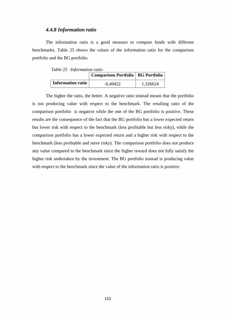
153
4.4.8 Information ratio
The information ratio is a good measure to compare funds with different
benchmarks. Table 25 shows the values of the information ratio for the comparison
portfolio and the BG portfolio.
Table 25 –Information ratio
Comparison Portfolio BG Portfolio
Information ratio -0,49422 1,326624
The higher the ratio, the better. A negative ratio instead means that the portfolio
is not producing value with respect to the benchmark. The resulting ratio of the
comparison portfolio is negative while the one of the BG portfolio is positive. These
results are the consequence of the fact that the BG portfolio has a lower expected return
but lower risk with respect to the benchmark (less profitable but less risky), while the
comparison portfolio has a lower expected return and a higher risk with respect to the
benchmark (less profitable and more risky). The comparison portfolio does not produce
any value compared to the benchmark since the higher reward does not fully satisfy the
higher risk undertaken by the investment. The BG portfolio instead is producing value
with respect to the benchmark since the value of the information ratio is positive.
154
Conclusions
This analysis wants to test the value generated by the investment management
company Morningstar Investment Management to a portfolio of mutual funds. The
reason why we are interested in the management of this specific company is its
innovative approach of portfolio creation through the optimization model Markowitz
2.0 and its innovative management approach of target volatility. Moreover, the company
is a division of Morningstar Inc., an investment research firm that supplies information,
classifications and ratings of mutual funds to the main online platforms. Consequently,
the investment management division of this society has several strengths with respect to
its competitors, having direct access to all the information of each fund.
Our analysis starts with the study of three portfolios of funds (funds of funds) of
the insurance company Clerical Medical, that are managed by Morningstar since March
2013. The portfolios, that have an increasing risk profile, are the CMIG Euro Cautious
Managed, the CMIG Euro Balanced Managed and the CMIG Euro Adventurous
Managed. The management process of the three portfolios is based on four basic steps:
strategic asset allocation, fund‘s selection, dynamic asset allocation and daily
monitoring. More specifically, Morningstar first defines the strategic asset allocation of
the portfolios and then chooses the funds to be included through a sophisticated analysis
of the style, capitalization, geographic and business sectors of investment of each fund
in order to create extremely diversified portfolios. The optimal portfolio is then chosen
according to the Markowitz 2.0 optimization approach (introduced by Kaplan and the
Morningstar research team). Moreover, Morningstar constantly monitors the portfolios
applying the target volatility asset allocation strategy, which implies the rebalancing of
the portfolio allocation between equity and bond funds to maintain the target portfolio
volatility.
In order to test the efficiency of the management of this professional investor,
we concentrate our attention on one of the three portfolios, the CMIG Euro Adventurous
155
Managed Portfolio, that is the one with the riskiest profile. We choose this portfolio
because we have a good proxy for it. The proxy is the fund BG Selection Global Risk
Managed AX, a fund of a SICAV of Generali Bank that has been managed by
Morningstar since October 2009 and so it has a more significant time frame to test
Morningstar management. Also the BG portfolio is managed with the target volatility
asset allocation approach.
To proceed with the analysis, we create a comparison portfolio whose date of
creation is October 2009, like the BG fund. The comparison portfolio is created
following the classical Modern Portfolio Theory by Markowitz, it is static and it invests
in the same asset classes of the Morningstar portfolio. The funds included in the
portfolio are selected in a way that, for each fund in the Morningstar portfolio, there is a
corresponding fund in the comparison portfolio that belongs to the same Morningstar
asset class. In order to create the optimal allocation of the funds in the portfolio, we use
a dataset that includes the returns of the funds selected in the time frame October 2004 –
September 2009. With the use of Excel we calculate the mean vector R and the
variance-covariance matrix Ω and with the Solver in Excel we solve the optimization
model that finds the vector of weights X that maximizes the expected return for a given
level of variance. Plotting the results on a mean-variance Cartesian plan and connecting
the points we graphically get the efficient frontier, that is the set of the portfolios that
maximize the returns for a given level of variance or, equivalently, that minimize the
variance for a given level of returns. The efficient frontier is calculated imposing the
only constraints that the weights sum up to one and that each weight is non-negative
(since we do not want short selling). Since the results are not satisfying as the resulting
weights concentrate on a few funds of the portfolio, we calculate the efficient frontier
another time imposing a further constraint. The added constraint imposes that the
weight of each fund is greater than 0,02 but smaller than 0,11. In this way none of the
weights is smaller than 2% and greater than 11%, like in the portfolio created by
Morningstar. The second efficient frontier is lower and shifted to the right in the mean-
variance plan but it provides more significant results for the purpose of our analysis.
Once the efficient frontier is determined, we find the optimal portfolio
maximizing the Sharpe ratio. The optimal portfolio corresponds to the point of tangency
between the straight line (that starts from the y-axis at the risk free rate) and the efficient
frontier in the expected return-standard deviation plan. Since we are supposing that the
156
investor invests his money only in our portfolio funds, he cannot choose a combination
of the risky portfolio and of the risk-free asset, but he invests just in the risky portfolio.
Thanks to this procedure we are sure that our portfolio is efficient. If our portfolio had
not been efficient since its creation, it would have been disadvantaged in relation to the
Morningstar portfolio.
Before carrying out our analysis we expected the performance of the comparison
portfolio to be lower than the one of the BG portfolio and we expected the BG portfolio
to produce more value to the investment than the comparison portfolio. The first
interesting result of our analysis lies in the optimal portfolio choice. With the funds that
we selected, it is not possible to create a portfolio with the same equity/fixed income
proportion of the Morningstar portfolio. Our portfolio in fact invests a lower percentage
in stock funds (49% equity funds and 51% fixed income funds) than the Morningstar
portfolio (65% equity funds and 51% fixed income funds –neutral allocation), keeping
in mind that the equity/fixed income asset allocation of the Morningstar portfolio is
subject to change according to the expected volatility of the market, while the asset
allocation of our portfolio is static.
Our first expectation is not realized. On absolute terms, the performance of the
comparison portfolio is higher than the one of the Morningstar portfolio. This is
evidenced by the higher expected returns and the higher cumulated returns that it
exhibits with respect to the Morningstar portfolio. However, it is important to notice
that the quality of the two investments differs on several aspects. The comparison
portfolio in fact has a lower percentage invested in stocks, a higher percentage invested
in Pacific area and Emerging markets funds, and it has a lower exposition to the dollar.
In the last two years the funds of the Asia Pacific and Emerging markets have
performed high returns and this might have contributed to improve the performance of
our comparison portfolio. In addition, the depreciation of the dollar in 2013 penalized
the performance of the Morningstar portfolio relatively to its category. Morningstar
strategy in fact envisages a high exposition to the dollar that for a European investor
functions as a natural hedge, since it covers a part of the losses when the markets go
down. In this way, Morningstar renounces to some profit when the markets go up but it
has lower losses when the markets go down. The combination of the well performing
Pacific Asia and Emerging Market funds and the depreciation of the dollar might have
played in favor of the performance of the comparison portfolio and against the BG
157
portfolio and we do not have enough information to state with certainty that the
comparison portfolio will have a higher performance also in the long run.
Since returns mean nothing unless compared to the risk undertaken to get that
return and since the performance and risk of mutual funds are meaningful only if
compared to the benchmark of reference, we proceed our study deriving information
over the performance adjusted to the risk and with the comparison of the performance
and risk of the fund relatively to the benchmark of reference. The benchmark that we
use to evaluate the BG fund is the same used by Morningstar in its analysis (25%
Barclays Euro Aggregate Bond Index and 75% Ftse World Index) while the benchmark
used for the comparison portfolio is composed by the same indices but with different
percentages (50% Barclays Euro Aggregate Bond Index and 50% Ftse World Index)
since it is composed of a lower percentage of stocks.
We calculate the Sharpe ratio of the two portfolios to rank the reward to risk
with respect to benchmark of reference. The Sharpe ratio of both the portfolios is lower
than the Sharpe ratio of the corresponding benchmark, this means that each of the two
funds has a lower return to variability with respect to the benchmark. Anyhow, the two
Sharpe ratios are positive and so both the portfolios are rewarding in a certain measure
the risk that they are taking and they are not destroying value. Moreover, both the
portfolios are capable of rewarding the systematic risk of the investment since they have
a Treynor ratio greater than one, suggesting that they are producing more units of
returns than of risk. The Modigliani measure allows us to deduce that the portfolios
would perform less than the corresponding benchmark even if they had the same level
of risk of the benchmark. This is further confirmed by the value of the alpha that
evaluates the extra return provided by the investment above the expectation that the risk
procured, defining managers‘ ability of stock picking. The alpha of the two funds is
negative since they perform less than what expected. However, as most of the funds in
the same category are currently performing negative alphas, we consider that this value
might change in other market conditions.
Shifting the attention to the risk of the two investments, the portfolios have a
beta greater than one and so they are more risky than their benchmark. Moreover, if we
focus on the volatility (standard deviation) of the two portfolios, the volatility of the BG
portfolio is higher than that of the comparison portfolio in the short run while it is lower
in the long run. This proves that Morningstar succeeded in targeting the level of
158
volatility, controlling the risk and limiting the losses in the long term, while the
comparison portfolio does not keep volatility under control. We remember on this
subject that the main objective of the two funds is to beat the benchmark in the long run
and not in the short run.
Finally, the last index analyzed in our study is the information ratio that allows
us to compare the portfolios on the basis of the value added to each portfolio by the
management. The resulting ratio of the comparison portfolio is negative while the one
of the BG portfolio is positive. The negative ratio means that the comparison portfolio
does not produce further value compared to the benchmark (since it is less profitable
and more risky than the benchmark), while the positive ratio means that the BG
portfolio is producing value with respect to the benchmark (since it is less profitable but
less risky). Our second expectation is then satisfied, the fund managed by Morningstar
is producing more value to the investment than our comparison portfolio if we compare
the investments to the appropriate benchmark.
We can conclude that the portfolio that is professionally managed and constantly
monitored by Morningstar generates greater value than our static portfolio. Moreover,
the Morningstar portfolio is more successful in the long run, granting better results in
terms of reward to risk with respect to the benchmark. Relatively to this, it should be
kept in mind that the performance of a fund evaluated on its own, without taking into
consideration the risk and the benchmark, is not significant. So, even if the comparison
portfolio performs higher expected and cumulated returns, it is necessary to note that it
does not produce more value with respect to the benchmark.
159
Bibliography
Assogestioni (2011), ―Task force Assogestioni per l‘implementazione della riforma
della tassazione dei fondi comuni‖, Conclusive Document, Italy.
Anolli, M., A. Del Giudice (2008), “Italian Open End Mutual Fund Costs”, Università
Cattolica del Sacro Cuore, Working Paper n. 8111, Milan.
Bartiloro, L., C. Rampazzi (2013), “Questioni di Economia e Finanza- Il risparmio e la
ricchezza delle famiglie italiane durante la crisi”, Bank of Italy, European System of
Central Banks, Occasional Working paper 148.
Baselli, V. (2014), ―La volatilità fa la performance‖, Morningstar.it,
http://www.morningstar.it/it/news/78125/la-volatilit%C3%A0-fa-la-
performance.aspx.
Beltratti, A., R. Miraglia (2001), I fondi comuni di investimento, Carocci editore, Rome.
Black, F., R. Litterman (1992), ―Global Portfolio Optimization, Financial Analysts
Journal, 28-43.
Blake, C. R., M. R. Morey (2000), Morningstar Ratings and Mutual Fund Performance,
Journal of Financial and Quantitative Analysis, 35, 451-483.
Blume, M (1998), ―An Anatomy of Morningstar Ratings‖, Financial Analysts Journal,
54: 1-9.
Brinson, G.P.,B.D. Singer, G.L. Beebower (1991), ―Determinants of Portfolio
Performance II: An Update‖, Financial Analysts Journal, 47: 3: 40-48.
Campbell J. Y., L. M. Viceira (2002), Strategic Asset Allocation –Portfolio Choice for
Long-Term Investors, Oxford University Press, New York.
Castagna, D., ―Oltre gli alti e bassi del mercato: i nuovi fondi Managed‖, public speech
in the Roadshow Clerical Medical, May 2013.
Castagna, D., ―I Fondi Managed, in rete con il gestore‖, speech in the Webinar Clerical
Medical, December 2013.
Cesari R., F. Panetta (2002), ―The performance of Italian equity funds‖, Journal of
Banking & Finance, 26: 99-126.
Chamberlain, G. (1983), ―A characterization of the distributions that imply mean-
variance utility functions‖, Journal of Economic Theory, 29: 185-201.
160
Chew Leong (2011), ―Target Volatility Asset Allocation Strategy‖, Societies of
Actuaries, article from International News, Issue 53.
Daniel, K. D., D. Hirshleifer, A. Subrahmanyam (2001), ―Overconfidence, Arbitrage,
and Equilibrium Asset Pricing‖, Journal of Finance, 38: 745-752.
Del Guercio, D., P. A. Tkac (2001), ―Star Power: The Effect of Morningstar Ratings on
Mutual Fund Flows‖, Federal Reserve Bank of Atlanta, Working Paper 2001-15.
De Marchi, G., G. Roasio (1999), I fondi comuni di investimento. Come funzionano.
Quando convengono, Il Sole 24 Ore S.p.a., Milan.
EFAMA (2013), ―Asset Management in Europe –Facts and Figures‖, 6th
Annual
Review, EFAMA, June 2013.
Fama, E. (1965), ―The behavior of stock-market prices‖, Journal of Business, 38: 34-
105.
Fernando, D., L. Klapper, V. Sulla and D. Vittas (2003), ―The Global Growth of Mutual
Funds‖, World Bank Polocy Research, Working Paper 3055.
Francis J. C., D. Kim (2013), Modern Portfolio Theory, + Website, Foundations,
Analysis, and New Developments, First Edition, Wiley Finance, New Jersey.
Fredman, A. J., R. Wiles (1993), How mutual funds work, New York Institute of
Finance, New Jersey.
Gibson, R. C. (1990), Asset Allocation: Balancing Financial Risk, Dow Jones-Irwin,
Homewood.
Hight, N.G. (2010), ―Diversification effect: Isolating the Effect of Correlation on
Portfolio Risk‖, Journal of financial planning, 23: 5: 54.
Hübner, G. (2005), “The Generalized Treynor Ratio”, Springer, 9: 415-435.
Ibbotson, R.G., P. Kaplan (2000) ―Does Asset Allocation Policy Explain 40, 90, or 100
Percent of Performance?‖, Association for Investment Management and Research,
26-33.
Ippolito, R. A. (1989), ―Efficiency with costly information: A study of mutual fund
performance, 1965-1984‖, The Quarterly Journal of Economics, 104: 1: 1-23.
Jensen, M.C. (1968), ―The performance of mutual funds in the period 1945-1964‖,
Journal of Finance, 23: 2: 389-416.
Jorion, P. (1991), ―Portfolio Properties of the ECU‖, Journal of Multinational Financial
Management, 1-24.
161
Kaplan, P. D., T. Idzorek, M. Gambera, K. Yamaguchi, J. Xiong, D. M. Blanchett
(2009), ―The History and Economics of Stock Market Crashes‖, Insights into the
Global Financial Crisis, ed. L. B. Siegel, CFA institute, 132-169.
Kaplan, P. D. (2011), Frontiers of Modern Asset Allocation, Wiley Finance.
KPMG Advisory S.p.a. (2012), ―Risparmio gestito in Italia: trend ed evoluzione dei
modelli di business”, Italy.
Levy, H., H. Markowitz (1979), ―Approximating Expected Utility by a Function of
Mean and Variance, The American Economic Review, 69: 3: 308-317.
Levy, M, R. Roll (2009), ―The Market Portfolio May Be Mean-Variance Efficient After
All‖, The Review of Financial Studies 23: 6: 2464-2491.
Liberty, J (2010), ―Geometric Information Ratio‖, Au.Tra.Sy blog - Automated Trading
System, http://www.automated-trading-system.com/geometric-information-
ratio/#start.
Lintner, J. (1965), ―The Valuation of Risky Assets and the Selection of Risky
Investments in Stock Portfolios and Capital Budget‖, Review of Economics and
Statistics, 47: 13-37.
Luenberger D. G. (2006), Finanza e investimenti –Fondamenti matematici, Italian
edition S. Scarlatti, Apogeo, Milan (original: Investment Science, Oxford University
Press, New York, 1998).
Maginn, J. L., D. L. Tuttle, J. E. Pinto, D. W. McLeavey (2007), Managing Investment
Portfolios: A Dynamic Process, Third Edition, CFA Institute, New Jersey.
Manganelli S., R. F. Engle (2001), ―Value At Risk Models in Finance‖, European
Central Bank, Working paper 2001-75.
Mandelbrot, B., R. L. Hudson (2004), The (Mis)Behaviour of Markets: A Fractal View
of Risk, Ruin, and Reward, Profile Books, London.
Malkiel, B. G. (2003), A Random Walk Down Wall Street: The Time Tested Strategy for
Successfu Investing (completely revised and updated), W.W. Norton & Company,
New York.
Markowitz H. (1952), ―Portfolio Selection‖, Journal of Finance, 7: 1: 77-91.
Mausser H., D. Rosen (2002), ―Scenario-Based Risk Management Tools‖, Algorithmics
Incorporated, Toronto, Canada.
Modigliani F., L. Modigliani (1997), ―Risk-Adjusted Performance‖, Journal of
Portfolio Management, 45-54.
Morey, M. (2000), ―Mutual Fund Age and Morningstar Ratings‖, Pace University,
Working Paper.
162
Morningstar (2009), ―The Morningstar Rating Methodology‖, Morningstar, Inc.,
Morningstar Methodology Paper.
Mossin, J. (1966), ―Equilibrium in a Capital Asset Market‖, Econometrica, 34: 768-783.
Neumann, J. V., O Morgenstern (1947), Theory of Games and Economic Behavior,
Second Edition, Princeton University Press, New Jersey.
Owen, J., R. Rabinovitch (1983), ―On the class of elliptical distributions and their
applications to the theory of portfolio choice‖, Journal of Finance, 3: 745-752.
Plantier, L. C. (2014), ―Globalisation and the Global Growth of Long-Term Mutual
Funds‖, ICI Global Research Perspective 1, n.1, March.
Roll, R. (1977), ―A Critique of the Asset‘s Pricing Theory‘s Tests: Part I‖, Journal of
Finance, 32 : 2 : 177-190.
Rose, G. (2014), ―How to Manage Volatility‖, Morningstar.co.uk,
http://www.morningstar.co.uk/uk/news/121264/how-to-manage-volatility.aspx
Ross, S. A., R. W. Westerfield, B. D. Jordan (2008), Corporate Finance Fundamentals,
Eight Edition, Mc Graw Hill International Edition, Singapore.
Santoboni F. (2012), Manuale di gestione assicurativa –Profili economici, finanziari e
di governance, Cedam, Lavis (TN).
Saunders, T., M. M. Cornett (2009), Financial Markets and Institutions, Fourth Edition,
Mc Graw Hill International Edition, New York.
Savage, S. (2009), The Flaw of Averages, John Wiley & Sons, Hoboken, NJ.
S&P (2012), ―S&P Dow Jones Indices: Float Adjustment Methodology‖, S&P Dow
Jones Indices, US.
Sharpe, W. (1964), ―Capital Asset Prices: a Theory of Market Equilibrium Under
Conditions of Risk‖, Journal of Finance,19: 3: 425-442.
Sharpe, W. (1966), ―Mutual Fund Performance‖, Journal of Business, 39: S1: 119-138.
Sharpe, W. (1994), ―The Sharpe Ratio‖, The Journal of Portfolio Management, 21:1:
49-58.
Sharpe, W. (1998), ―Morningstar‘s Risk-Adjusted Ratings‖, Financial Analyst Journal,
54: 21-33.
Sinn, H. W. (1983), Economic Decisions under Uncertainty, Second English Edition,
North Holland, Amsterdam.
Taleb, N. N. (2004), Fooled by Randomness, Random House, Inc., New York.

163
Thaler, R., N. Barberis (2002), ―A Survey of Behavioral Finance‖, Handbook of the
Economics and Finance, National Bureau of Economics Research.
Tobin, J. (1957), ―Liquidity Preference as Behavior towards Risk‖, Review of Economic
Studies, 54—86.
Waggoner, J., ―A star is reborn after shake-up‖, US Today, December, 2nd
2001.
Wang S., Y. Xia (2002), Portfolio Selection and Asset Pricing, Springer, Germany.
164
Bibliography of websites
Assogestioni website: www.assogestioni.it (last access: May 2014)
BG Selection Sicav KIID (Key Investor Information Document:
file:///C:/Documents%20and%20Settings/Utente/Documenti/Downloads/6003951BG_B
GSelectionSi.pdf (last access: June 2014)
Bloomberg database and website: www.bloomberg.com
Clerical Medical website: www.clericalmedical.com (last access: June 2014)
Consob website: www.consob.it (last access: March 2014)
Efama website: www.efama.org (last access: April 2014)
Forexmarket: www.forexmarkethours.com (last access: May 2014)
Generali Bank website: www.bancagenerali.it (last access: June 2014)
Il Sole 24 ore: www.ilsole24ore.com (last access: May 2014)
Invesco Ltd website: www.invesco.com (last access: May 2014)
Investopedia: www.investopedia.com (last access: June 2014)
Morningstar website: www.morningstar.it (last access: June 2014)
Performance Trading: www.performancetrading.it (last access: May 2014)
Prometeia website: www.prometeia.it (last access: March 2014)
Reuters website: www.reuters.com (last access: May 2014)
Sewell, M. (2010), ―Behavioural Finance‖: www.behaviouralfinance.net (last access:
April 2014)