Management Modeling of

Suspended Solids and Living

Resource Interactions

Carl Cerco1, Mark Noel1, Sung-Chan Kim2

1Environmental Laboratory, US Army ERDC, Vicksburg MS, USA2Coastal and Hydraulics Laboratory, US Army ERDC, Vicksburg

MS, USA

Contact Information: Carl F. Cerco, Environmental Laboratory, US Army ERDC, 3909 Halls Ferry Road, Vicksburg MS 39180, USA;

Phone 601-634-4207; Fax 601-634-3129; email: Carl.F.Cerco@usace.army.mil

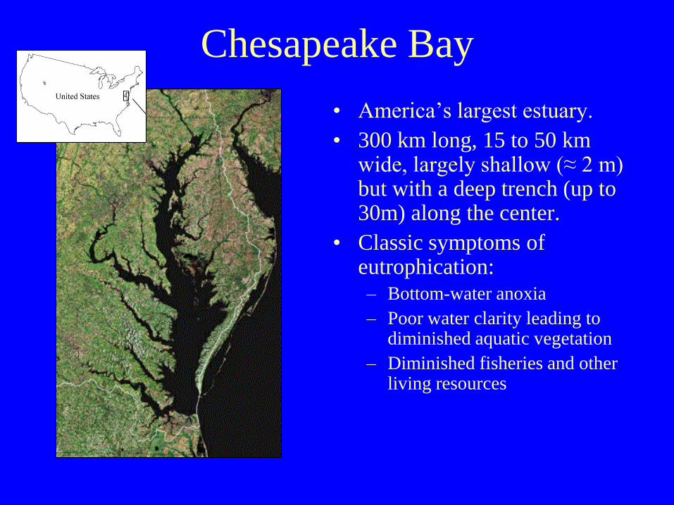
Chesapeake Bay

• America’s largest estuary.

• 300 km long, 15 to 50 km wide, largely shallow (≈ 2 m) but with a deep trench (up to 30m) along the center.

• Classic symptoms of eutrophication:

– Bottom-water anoxia

– Poor water clarity leading to diminished aquatic vegetation

– Diminished fisheries and other living resources

Regional

Atmospheric

Deposition

Model

Benthos

Component

Watershed

Model

Hydrodynamic

Model

Eutrophication

Model

SAV

Component

The CBEMP

Submerged Aquatic Vegetation

• SAV is limited to shallow water

(< 2 m) and littoral zones.

• SAV distribution and

abundance are determined by

numerous factors. Light is the

foremost of these.

• Restoration of SAV to its

1950’s level is a goal of the

Chesapeake Bay Program.

• Image courtesy of Virginia

Institute of Marine Science.

SAV Sub-Model

Schematic of SAV Model

Components

SAV Model Sub-Grid

Attenuation by Colored

Dissolved Organic

MatterAttenuation by

Particulate Organic

Matter

Surface Irradiance

Attenuation by

Inorganic Solids

Attenuation by

Attached Epiphytes

Reflection

20% of Surface

Irradiance

Required by SAV

Sources of Light Attenuation

Freshwater - Saltwater

Freshwater - Saltwater

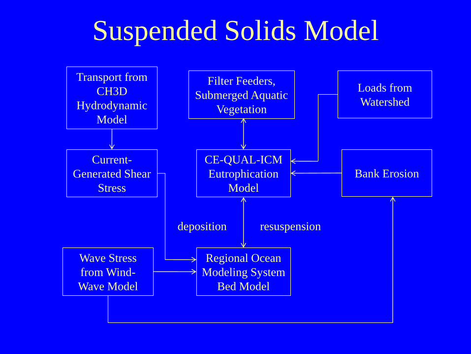
Suspended Solids Model

CE-QUAL-ICM

Eutrophication

Model

Regional Ocean

Modeling System

Bed Model

Filter Feeders,

Submerged Aquatic

Vegetation

resuspensiondeposition

Bank Erosion

Loads from

Watershed

Wave Stress

from Wind-

Wave Model

Transport from

CH3D

Hydrodynamic

Model

Current-

Generated Shear

Stress

Bottom Shear Stress, Bank Erosion

Percent of time that bed shear stress is

dominated by currents. (After Harris et al.

2010)

Shoreline Erosion

KG/M/Day

0.0 - 0.5

0.6 - 1.0

1.1 - 3.0

3.1 - 5.0

5.1 - 100.0

Long-term average shoreline erosion in

the Chesapeake Bay system (From

Halka and Hopkins 2006).

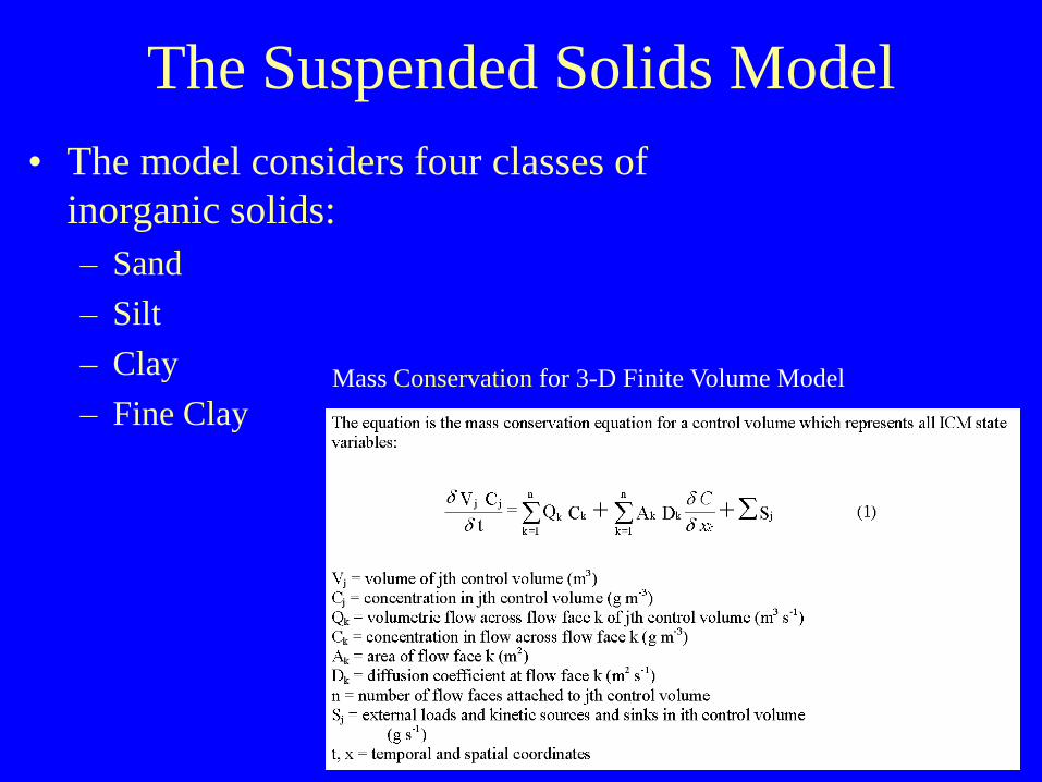
The Suspended Solids Model

• The model considers four classes of

inorganic solids:

– Sand

– Silt

– Clay

– Fine ClayMass Conservation for 3-D Finite Volume Model

Suspended Solids Model

Erosion and Deposition at Sediment-Water Interface

Continuous Deposition through Water Column

Suspended Solids Model

Erosion of Sand

Erosion of Clays and Silt

Light AttenuationLight Attenuation Model Based on Inherent Optical Properties

Field program

to measure

optical

properties.

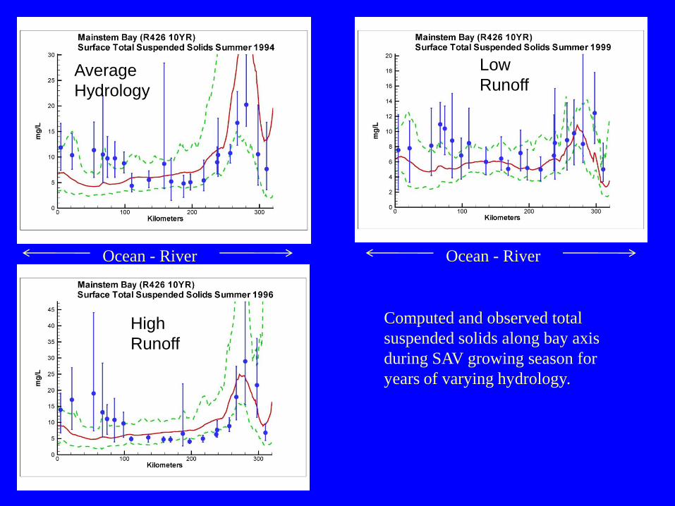
Computed and observed total

suspended solids along bay axis

during SAV growing season for

years of varying hydrology.

Ocean - River Ocean - River

Average

Hydrology

High

Runoff

Low

Runoff

Computed and observed light

attenuation along bay axis

during SAV growing season for

years of varying hydrology.

Ocean - River Ocean - River

Average

Hydrology

High

Runoff

Low

Runoff

Ten-year time series of

computed and observed total

suspended solids at three

locations along bay axis.

Upper Bay

Middle

Bay

Lower Bay

Ten-year time series of

computed and observed total

suspended solids at three

locations along bay axis.

Upper Bay

Middle

Bay

Lower Bay

SAV Restoration Scenarios -

Background

• The goal of the Bay Program is

to restore SAV to the 2m depth

contour.

• This roughly represents the

distribution circa 1950.

• Watershed loads of nutrients

and solids were much lower

than. As an approximation we

use 10% of present levels.

• We examine the individual and

combined response to 90%

reductions in nutrient and solids

loads.

Percent Improvement in Area of

SAV Beds

90% Nutrient Reduction 90% Solids Reduction Nutrient and Solids Reduction

Improvements in

middle to lower

portions of systems.

Improvements near

watershed inputs.

Management has

little effect on the

extreme lower bay.

Conclusions

Model

• The model reproduces the

basic solids distribution and

the major processes that

affect solids.

• We have moved in the right

direction by incorporating

solids in the eutrophication

model.

• The model is “ahead” of the

data in terms of biological

feedbacks, observations of

solids, and solids processes.

Aquatic Vegetation

• The largest fraction of light

attenuation originates in

high inorganic solids

concentrations.

• Inorganic solids respond to

load controls primarily near

local loading sources from

the watershed.

• SAV in the mid-bay and

lower tributaries responds to

reduction of organic solids

and epiphytes achieved via

nutrient controls.