האוניברסיטה העברית בירושליםThe Hebrew University of Jerusalem

המחלקה לכלכלה חקלאית ומנהלThe Department of Agricultural

Economics and Management

המרכז למחקר בכלכלה חקלאיתThe Center for Agricultural

Economic Research

Discussion Paper No. 3.07

The Stabilization Value of Groundwater and Conjunctive Water Management

Under Uncertainty

by

Masahiko Gemma and Yacov Tsur

מאמרים של חברי המחלקה נמצאים :גם באתרי הבית שלהם

Papers by members of the Department can be found in their home sites:

http://departments.agri.huji.ac.il/economics/indexe.html

76100רחובות , 12. ד.ת P.O. Box 12, Rehovot 76100

brought to you by COREView metadata, citation and similar papers at core.ac.uk

provided by Research Papers in Economics

The Stabilization Value of Groundwater and Conjunctive Water Management under Uncertainty*

Masahiko Gemma1 and Yacov Tsur2

The importance of managing ground and surface water conjunctively increases

with water scarcity and with inter- and intra-temporal fluctuations in precipitations. Both

factors are becoming critical in many parts of the world: the former due to increased

water demand associated with economic and population growth; the latter due to climate

change. A conjunctive ground and surface water system appears in a number of forms,

which differ according to the ground and surface water sources. Surface water may

consist of stream flows emanating from aquifers, surface reservoirs or lakes, snowmelt,

rainfall or any combination of these. It may be stable or stochastically fluctuate over

time. Groundwater sources – aquifers – may be non-replenishable or replenishable, deep

or shallow, confined or unconfined. The two cases in which only surface water or only

groundwater is used lie on both ends of the conjunctive spectrum; these extreme cases

occur when one source is always cheaper than the other (scarcity cost included).

Conjunctive systems, viewed in this larger context, characterize most irrigation systems

worldwide. The term conjunctive signifies that the ground and surface water sources are

two components of one system and should be managed as such.

The analysis of conjunctive water systems was pioneered by Oscar Burt more

than 40 years ago. More recently, Tsur, Tsur and Graham-Tomasi, Provencher and Burt,

and Knapp and Olson extended the theory to account for stochastic, dynamic and

multiaquifer considerations. The underlying idea is simple. Surface water sources

derived from rainfall and snowmelt typically fluctuate randomly from year to year and * This paper was presented at the Session "New frontiers in water economics," ASSA annual meeting, Chicago, Jan 5-7, 2007. 1 Masahiko Gemma is a professor at Waseda University, Japan. 2 Yacov Tsur is a professor at the Hebrew University of Jerusalem, Israel.

within a year. Groundwater stocks, on the other hand, are relatively stable because the

slow subsurface flows tend to smooth out intra- and inter-temporal fluctuations.

Groundwater thus performs a dual function, increasing the mean and reducing the

variability of total water supply. The value of groundwater is usually attributed to its first

– mean increasing – role, while its variability reducing role is ignored. Yet the latter role

carries an economic value, which is designated as the stabilization value (or buffer values

in the dynamic context) of groundwater, which could be substantial.

Why should we be interested in the stabilization value as a distinct concept?

Suppose that a groundwater development project can be implemented at some cost and

the decision whether or not to undertake the project is based on a cost-benefit criterion.

Clearly, determining the benefit generated by the groundwater project assuming that

surface water is stable at the mean, while easier to obtain, ignores the stochastic

fluctuations of surface water and the ensuing stabilization role of groundwater. If the

economic value associated with this role – the stabilization value – is non-negligible,

compared to the value of the resource due to increasing the mean water supply, this

simpler approach leads to a serious underestimation of the groundwater benefit and bias

assessment of the groundwater projects. Empirical studies (Tsur) reveal substantial

stabilization value of groundwater.

Here we discuss implications of the stabilizing role of ground water for

conjunctive ground and surface water policies. Applying the analysis to Coimbatore

Water District in Tmil Nadu, India reveals a substantial stabilization value. We conclude

with some remarks regarding the important role of conjunctive water management

policies in a world of increasing food demands and declining irrigation water supplies.

2

The stabilization value of groundwater revisited

Suppose that crop production requires only water and let f(x) be the per-hectare

yield-water response function, with x representing water input (the empirical application

employs an extended version with multiples outputs and inputs). The water response

function f(x) is assumed increasing and strictly concave over the appropriate range of

water input, reflecting the diminishing marginal productivity property. Let R(x) = pf(x)

represent revenue per hectare when output price is p (assumed exogenous to farmers).

Following the properties of the yield-water response function, f(x), the revenue function,

R(x), is increasing and strictly concave in water input.

Let S represent available surface water supply (e.g., annual rainfall), assumed to

fluctuate randomly according to some probability distribution function F(S). (We ignore

intra-seasonal variations of surface water and consider only variations in total supply of

surface water during a year.) When surface water (rainfall, stream flows emanating from

snow melt) is the only source of irrigation water, the revenue (which is also profit in this

case) R(S) also fluctuates randomly around its mean Rm=E{R(S)}, where E represents

expectation with respect to the distribution of S. If rainfall could be stabilized at the

mean Sm=E{S}, the revenue would have changed to R(Sm). Since R(⋅) is strictly concave,

we have (Jensen's inequality)

E{R(S)} < R(Sm). (1)

Let Sce be the Certainty-Equivalent water input satisfying

E{R(S)} = R(Sce), (2)

i.e., Sce is the constant annual surface water that leaves farmers indifferent between

receiving it with certainty (every year) and facing the uncertain rainfall S with

distribution F(S). Since R(⋅) is increasing, (1) and (2) imply Sce<Sm. (Growers are

3

assumed to be risk neutral and the divergence between Sce and Sm stems from the

concavity of the revenue function.)

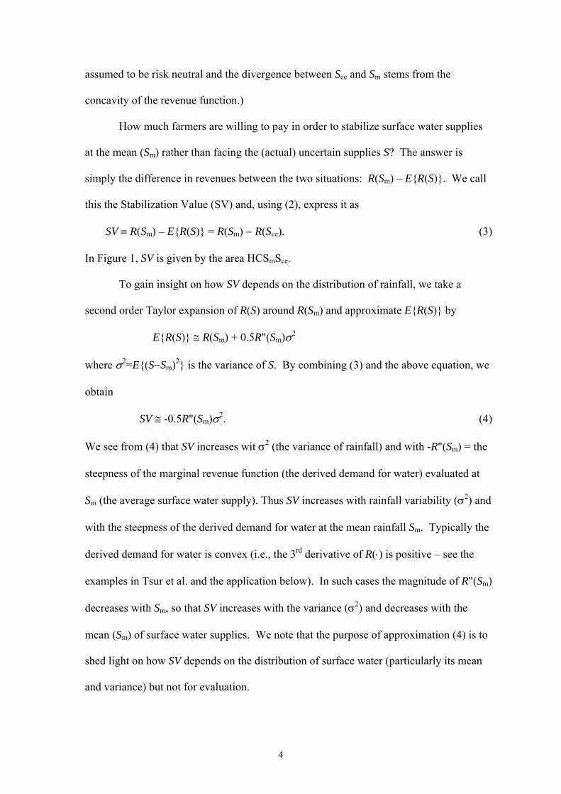
How much farmers are willing to pay in order to stabilize surface water supplies

at the mean (Sm) rather than facing the (actual) uncertain supplies S? The answer is

simply the difference in revenues between the two situations: R(Sm) – E{R(S)}. We call

this the Stabilization Value (SV) and, using (2), express it as

SV ≡ R(Sm) – E{R(S)} = R(Sm) − R(Sce). (3)

In Figure 1, SV is given by the area HCSmSce.

To gain insight on how SV depends on the distribution of rainfall, we take a

second order Taylor expansion of R(S) around R(Sm) and approximate E{R(S)} by

E{R(S)} ≅ R(Sm) + 0.5R"(Sm)σ2

where σ2=E{(S−Sm)2} is the variance of S. By combining (3) and the above equation, we

obtain

SV ≅ -0.5R"(Sm)σ2. (4)

We see from (4) that SV increases wit σ2 (the variance of rainfall) and with -R"(Sm) = the

steepness of the marginal revenue function (the derived demand for water) evaluated at

Sm (the average surface water supply). Thus SV increases with rainfall variability (σ2) and

with the steepness of the derived demand for water at the mean rainfall Sm. Typically the

derived demand for water is convex (i.e., the 3rd derivative of R(⋅) is positive – see the

examples in Tsur et al. and the application below). In such cases the magnitude of R"(Sm)

decreases with Sm, so that SV increases with the variance (σ2) and decreases with the

mean (Sm) of surface water supplies. We note that the purpose of approximation (4) is to

shed light on how SV depends on the distribution of surface water (particularly its mean

and variance) but not for evaluation.

4

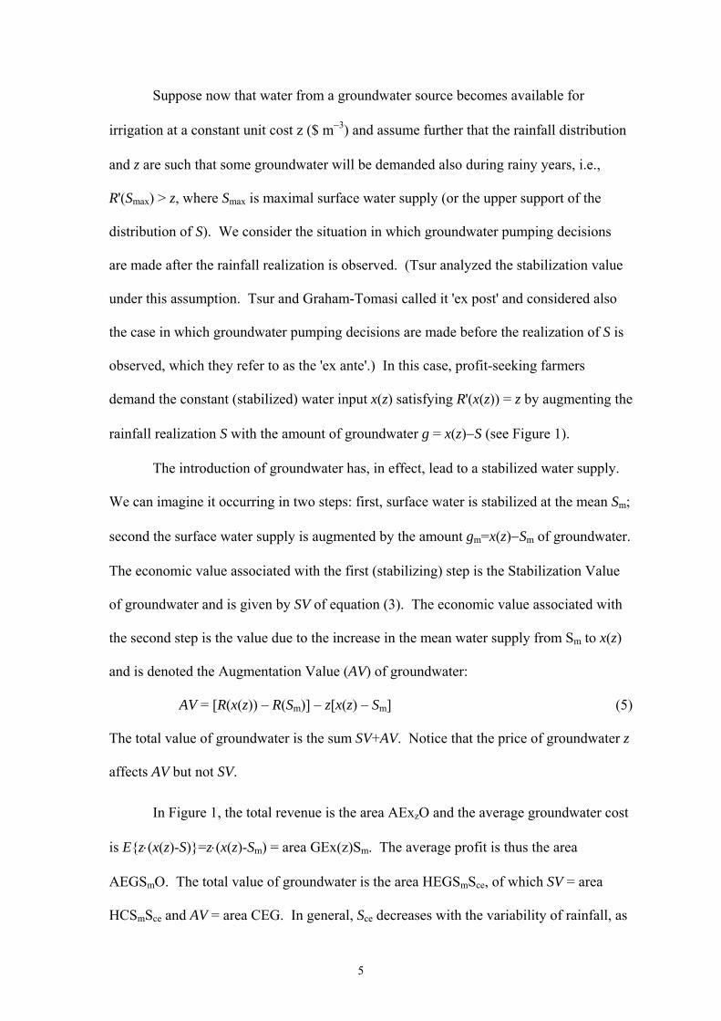
Suppose now that water from a groundwater source becomes available for

irrigation at a constant unit cost z ($ m−3) and assume further that the rainfall distribution

and z are such that some groundwater will be demanded also during rainy years, i.e.,

R'(Smax) > z, where Smax is maximal surface water supply (or the upper support of the

distribution of S). We consider the situation in which groundwater pumping decisions

are made after the rainfall realization is observed. (Tsur analyzed the stabilization value

under this assumption. Tsur and Graham-Tomasi called it 'ex post' and considered also

the case in which groundwater pumping decisions are made before the realization of S is

observed, which they refer to as the 'ex ante'.) In this case, profit-seeking farmers

demand the constant (stabilized) water input x(z) satisfying R'(x(z)) = z by augmenting the

rainfall realization S with the amount of groundwater g = x(z)−S (see Figure 1).

The introduction of groundwater has, in effect, lead to a stabilized water supply.

We can imagine it occurring in two steps: first, surface water is stabilized at the mean Sm;

second the surface water supply is augmented by the amount gm=x(z)−Sm of groundwater.

The economic value associated with the first (stabilizing) step is the Stabilization Value

of groundwater and is given by SV of equation (3). The economic value associated with

the second step is the value due to the increase in the mean water supply from Sm to x(z)

and is denoted the Augmentation Value (AV) of groundwater:

AV = [R(x(z)) – R(Sm)] – z[x(z) – Sm] (5)

The total value of groundwater is the sum SV+AV. Notice that the price of groundwater z

affects AV but not SV.

In Figure 1, the total revenue is the area AExzO and the average groundwater cost

is E{z⋅(x(z)-S)}=z⋅(x(z)-Sm) = area GEx(z)Sm. The average profit is thus the area

AEGSmO. The total value of groundwater is the area HEGSmSce, of which SV = area

HCSmSce and AV = area CEG. In general, Sce decreases with the variability of rainfall, as

5

can be seen from (2) and (4). Thus, a mean-preserving spread of the rainfall distribution,

which increases variance while keeping the mean intact, will increase the SV of

groundwater and vice-versa.

Figure 1 here

In actual practice multiple crops and multiple inputs exist and the derived demand

for irrigation water is modified accordingly. The SV of groundwater is then calculated as

explained above, using the aggregate derived demand for water. The framework can be

extended to multiple water storage sources, such as multiple aquifers with varying

pumping costs and surface reservoirs. Moreover, some of the water storage sources may

also be stochastic. As long as they are not perfectly correlated with rainfall they are

capable of affecting the variability of water supply in a way that gives rise to a

stabilization value.

Ignoring the rainfall variability, by assuming that rainfall is stable at the mean,

amounts to assuming that SV=0, which does away with the stabilizing role of

groundwater. This may lead to severe undervaluation of groundwater and distort water

management policies. Some policy implications are discussed in the next section,

followed by an empirical assessment of the stabilization value of groundwater in the

Coimbatore water district of Tamil Nadu, India.

Conjunctive management

The stabilization value of groundwater affects water policies in a number of ways.

First it affects the optimal extraction decisions of a dynamic exploitation policy. To see

this, consider the above conjunctive ground and surface water system over a long period

of time. Denote the aquifer's stock at time t by Gt, which evolve in time according to

dGt/dt = M(Gt) – gt, (6)

6

where M(G) is natural recharge, assumed non-increasing and concave in the aquifer's

stock G, and time is taken to be continuous. The aquifer management problem entails

finding the pumping policy {gt, t≥0} that maximizes the value

∫∞

−−+=0

rtttttt}{g0 dte]g)z(G)}g{R(S[Emax)V(G

t (7)

subject to (6), given initial stock G0 and feasibility constraints (gt≥0, Gt≥0), where r is the

time rate of discount and pumping cost z(G) may depend on the aquifer's stock. The

expectation Et is conditional on the realization of St being observed before the pumping

decision gt is made – a situation called 'ex-post' by Tsur and Graham-Tomasi .

A detailed analysis of this model can be found in Tsur and Graham-Tomasi

(1991). Here we just note the condition

R'(St+gt) = z(Gt) + V′(Gt) , (8)

determining the optimal pumping decision at time t, where V′(Gt) is the incremental

value due to marginal chance in the groundwater stock Gt or the shadow price of

groundwater (also known as user cost, in-situ value and scarcity value). (The expectation

is ignored because the realization St is assumed to be observed when gt is chosen.)

If, however, surface water is assumed stabilized at the mean, the management

problem changes to

∫∞

−−+=0

rttttm}{g0

m dt]e)gz(G)g[R(Smax)(GVt

(9)

subject to (6) and feasibility (e.g., nonnegativity) constraints and the optimal pumping

rule (8) becomes

R'(Sm+gt) = z(Gt) + V m′(Gt), (10)

Where V m′(Gt) is the groundwater shadow price when St is fixed at the mean Sm.

Tsur and Graham-Tomasi showed (under certain conditions) that

7

V ′(Gt) > V m′(Gt). (11)

The shadow price of groundwater under stochastic surface water supplies is larger

because of the added role of groundwater in stabilizing water supply and the ensuing

economic value that goes with it. Thus, at any given groundwater stock G, water users

should pay more for the resource, hence pump less, under stochastic rainfall relative to a

stabilized situation.

The Stabilization Value can also have a considerable effect on cost-benefit

analyses of groundwater projects. Quite often the mere access to an aquifer requires

investment in infrastructure, besides the operational costs associated with water pumping

and conveyance. This cost should be compared to the benefit associated with developing

the aquifer. Ignoring the stabilization value leads to underestimating the benefit

associated with the development project. To see this consider the case where extraction

cost z is independent of the stock and the aquifer stock is at a steady state, i.e., average

extraction just equals recharge: E{g(S)}=M(G). In this case the shadow price of

groundwater vanishes at a steady state (see Tsur and Graham-Tomasi) and Condition (8)

implies that S+g(S)=Sm+M(G). The value V(G) evaluated at a steady state is thus given

by

rGzMSRGMSR

rSR

rGzMGMSR

dteGzMGMSRdteSzgSgSREGV

mmmm

rtm

rt

)()())(()()())((

)())(()}())(({)(00

−−++=

−+=

−+=−+= ∫∫∞

−∞

−

The present value without groundwater is simply

.)}({)}({0 r

SREdteSREV rtS ∫∞

− ==

Thus, the benefit associated with developing the aquifer is

.)()())(()}({)()(r

GzMSRGMSRr

SRESRVGV mmmS −−++

−=−

8

The first term on the right-hand side is the present value of the Stabilization Value of

ground water. The second term is the present value of the Augmentation Value of

groundwater. Assuming stable surface water supplies is equivalent to assuming that SV

equals zero, hence biases downward the project's benefit. The magnitude of the bias

depends on the magnitude of SV. In 2 applications, the SV as a share of the total value of

groundwater was found to be substantial (Tsur). We turn now to calculate the

stabilization value of groundwater in the Coimbatore water district, located in Tamil

Nadu, India.

Application

Data: Irrigation water is derived from surface reservoirs, filled by the monsoon rains and

distributed via a system of canals, and from local aquifers. During the 2001-2002

agricultural year (that extends from July to June) 52.5% of the irrigation water came from

surface sources, 45.2% from local wells (groundwater) and the remaining 2.3% from

other sources (Palanisami).

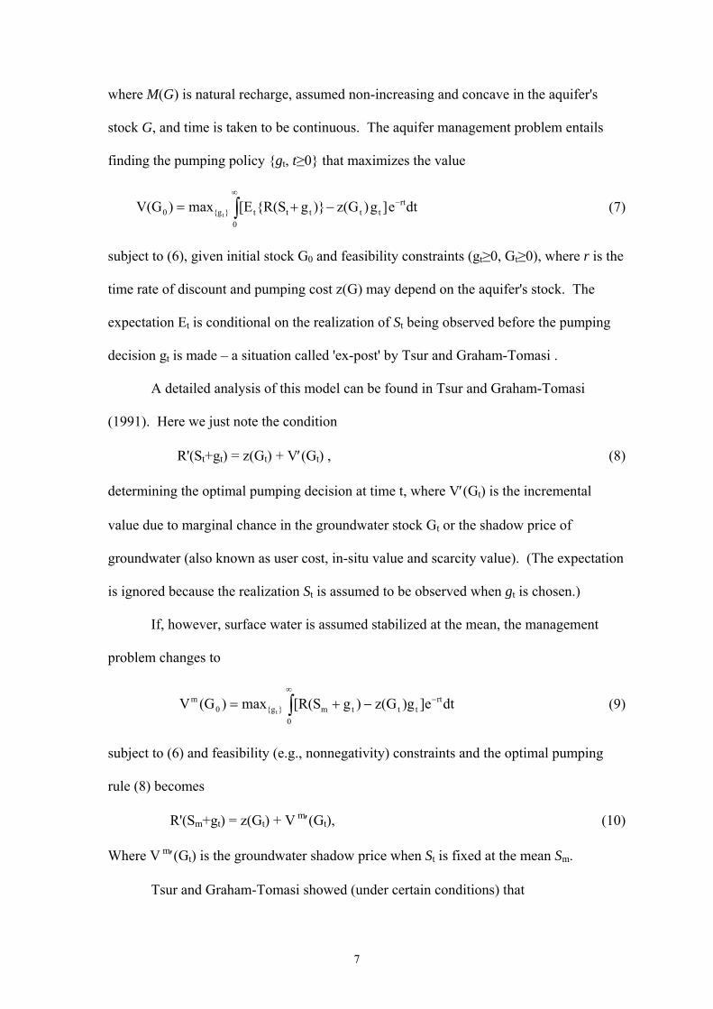
There are two monsoon periods: the Southwest monsoon from June to September;

and the Northeast monsoon from October to December. The period between January and

May is dry, but surface reservoirs allow distributing water throughout the year. The

annual rainfall, thus, constitutes the available surface water supplies. Figure 2 shows

annual rainfall data (mm) for the periods 1965-1985 and 1991-1999.

Figure 2 here

Due to rising water demands by non-agricultural users, the reservoirs now satisfy

about 90% of the irrigated area in normal year and only 60% during dry (low rainfall)

years. These shares are expected to worsen (decline) in the future, as urban, industrial

and environmental water demands rise. Thus, surface water supplies available for

9

irrigation will on average decline and become more variable (larger variance) in the

future (both trends increase the stabilization value of groundwater).

Crop pattern: Table 1 presents the main crops grown in Coimbatore District with their

cultivated area, water requirement (m3 ha-1), yield (100kg ha-1) and price (Rs per 100kg)

during the 2001-2002 agricultural year ($1=48.5 Rs in 2002). The main crops (in terms of

area) are ground nuts, paddy rice and sugar cane. The cultivation of ground nuts is done

during the dry season, while paddy is grown during the monsoon seasons. The only

perennial crop is Tapioca (most banana and sugar cane areas are replanted every year in

Coimbatore District). The most water intensive crops are sugar cane and banana

followed by paddy rice.

Table 1 here

Production inputs and cost: Table 2 lists the input requirements per hectare (other

than water) and their costs (Rs ha-1) for the 13 crops listed in Table 1 (since water is

assumed the binding constraint and not land, the cost of land is virtually nil). The

rightmost column of Table 2 gives the per hectare production cost, excluding water.

We turn now to calculate the stabilization value of groundwater in Coimbatore

Water District.

Table 2 here

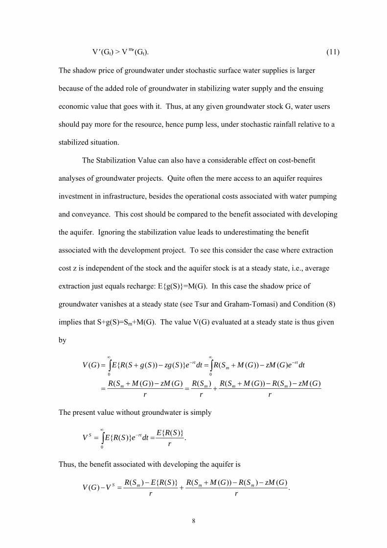
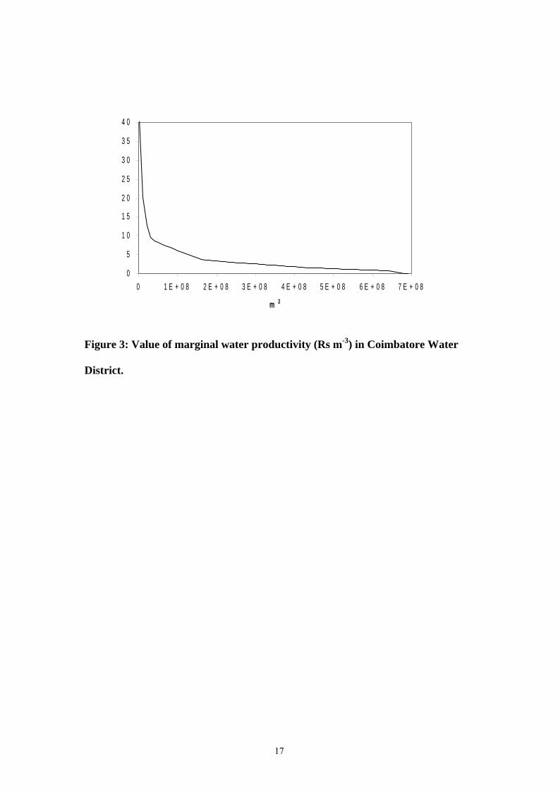
The Stabilization Value: The first step is to obtain the derived demand for irrigation

water. The aggregate data presented above do not permit detailed analysis and we follow

the approach used in Tsur et al., which utilizes Howitt's PMP method. Table 1 contains

data on crop area allocation, yield water requirements and output prices for the 13 crops

grown in Coimbatore district. Table 2 contains per hectare input requirements of all

production inputs other than water and their cost for these 13 crops. The rightmost

column summarizes the per hectare production cost, excluding water. . The data are then

processed by the PMP method to yield the derived demand for irrigation depicted in

Figure 3.

10

Figure 3 here

The rainfall data St, depicted in Figure 2, are measured in mm. The

corresponding surface water supplies are obtained by multiplying St by 10 times the

irrigated area (77543 ha).3 The rainfall distribution is taken as the empirical distribution

of the observed sample, where each observation receives an equal weight of 1/30 (30

being the number of observations).

For any water supply x, the revenue R(x) is calculated as the area beneath the

derived demand curve (Figure 3) to the left of x. In this way the revenues R(St),

t=1,2,…,30, are calculated for each observation (sampled year). The sample average

rainfall is Sm=ΣtSt/30 and R(Sm) is calculated as the area beneath the derived demand

curve to the left of Sm. Noting equation (3), obtaining SV requires the expected revenue

E{R(S)}, which we estimate by the sample mean ΣtR(St)/30. The Stabilization Value

(SV) is then estimated by

. (12) 30/)()(30

1∑=

−=t

tm SRSRSV

Calculating the Augmentation Value (AV) requires the cost of groundwater (cf.

equation (5)), which consists of the pumping and conveyance cost z(G) plus the user cost

(or in-situ value) λ (see equation (8)). Obtaining these costs requires solving the dynamic

optimization problem (7). This task requires elaborate hydrological and engineering

(pumping, conveyance) data and is beyond the present scope. To gain insight on the

share of SV in the total value of groundwater we calculate

A = R(∞) – R(Sm),

3 One mm rainfall over one hectare is equivalent to 10 m3.

11

which the AV when the cost of groundwater is zero. Thus, A > AV and

SV/(SV+AV) > SV/(SV+A). The share SV/(SV+A) is thus a lower bound on the share of

SV in the total value of groundwater.

The empirical results are presented in Table 3. Economic values are measured in

Rupees. We see that the stabilization value accounts for more than 25% of the total value

of groundwater. Ignoring it, by assuming stable rainfall, would have led to

underestimation of the value of groundwater by more than 25%.

Table 3 here

Concluding comments

Population growth and rising living standards lead to rapid increase in the

demand for water. Since the average quantity of renewable fresh water available for

use in any particular location is constant and water conveyance is an expensive

operation, water has become a scarce resource in many parts of the world. Adding the

prevalence of deteriorating water quality and the increased awareness for water-

related environmental and social problems helps to understand why water resource

management has become a critical policy challenge. In the region studied here,

surface water has been relocated away from irrigation to meet the growing demands

of other sectors in a way that reduces the average quantity of surface water available

for irrigation and at the same time increases its variability (the withdrawal for non-

agricultural uses is larger during dry years than during wet years).

Worldwide irrigation water still consumes the bulk of the available renewable

fresh water resources (over 70 percent). While irrigated agriculture is practiced on only

about 18 percent of total cultivable land (267 million hectare in 1997, of which 75

percent are in developing countries), it produces over 40 percent of agricultural output

(Gleick, World Bank). Irrigated area is expected to continue to expand in order to meet

12

the food demand of a growing population (FAO), but fresh water resources available for

irrigation will at best remain fixed and most likely decline, stressing the need for

improved efficiently of irrigation water.

There are ways to increase agricultural output without reliance on fresh water

sources, such as improved crop variety (genetically or conventionally modified),

appropriate water pricing and increased use of marginal sources (reclaimed, saline water).

In this work we focus on conjunctive management of ground and surface water. We note

that crop production is affected not only by the quantity of water input but also by how

this quantity is distributed within and between growing seasons. Owing to the random

nature of precipitations, surface water supplies typically fluctuate randomly while

groundwater sources are relatively more stable. The latter, thus, can be used to stabilize

the supply of irrigation water, thereby increasing output over and above that expected due

the increase in the average quantity of water input.

Applying the analysis to the Coimbatore district in Tamil Nadu, India, we found

that the stabilization value of groundwater exceeds 25% of the total value of

groundwater. Ignoring the stabilization value (by assuming that surface water is stable at

the mean) leads to undervaluing groundwater by more than 25%. Put differently, under

the prevailing rainfall variability, conjunctive management of ground and surface water

in this region can increase water use efficiency by more than 25%. Groundwater

resources are prevalent worldide, yet often mismanaged due to their common property

feature. This is particularly true for the region studied here (Palanisami). Understanding

the true value of groundwater is a necessary step towards a better management of this

resource.

13

References

Burt, O. "The Economics of Conjunctive Use of Ground and Surface Water, Hilgardia 36(1964): 31-111.

FAO, World Agriculture: Toward 2015/30, 2000.

Gleick, P. H., The world's water 2000-2001, Island Press, Washington, D.C., 2000.

Howitt, R. "Positive Mathematical Programming, American Journal of Agricultural Economics 77(1995): 329-342.

Knapp, K.C. and L.J. Olson. "The economics of conjunctive groundwater management with stochastic surface supplies," Journal of Environmental Economics and Management, 28(1995.): 340-356.

Palanisami, K. Tank Irrigation: Revival for Prosperity, Asian Publication Services, New Delhi, 2000.

Provencher, B. and O. Burt. "Approximating the optimal groundwater pumping policy in a multiaquifer stochastic conjunctive use setting," Water Resources Research 30(1994): 833-843.

Tsur, Y. "The Economics of Conjunctive Ground and Surface Water Irrigation Systems: Basic Principles and Empirical Evidence from Southern California, in D. Parker and Y. Tsur (eds) “Decentralization and Coordination of Water Resource Management”. Kluwer Academic Publishers: Boston, 339-361, 1997.

Tsur, Y. "The Stabilization Value of Groundwater when Surface Water Supplies are Uncertain: The Implications for Groundwater Development, Water Resources Research, 26(, 1990): 811-818.

Tsur, Y. and T. Graham-Tomasi "The Buffer Value of Groundwater with Stochastic Surface Water Supplies," Journal of Environmental Economics and Management, 21(1991): 201-224.

Tsur, Y., T. Roe, R. Doukkali and A. Dinar. Pricing Irrigation Water: Principles and Cases from Developing Countries, RFF Press: Washington, DC, 2004.

World Bank, World Development Report 2000/2001: Attacking Poverty, Washington/New York: World Bank/Oxford University Press, 2001.

14

H

GF

ED

C

B

A

O

R'(x)

Smin

Dry years Smax

Wet years Sm

Average

z

$/m3

m3X(z)=S+g Sce

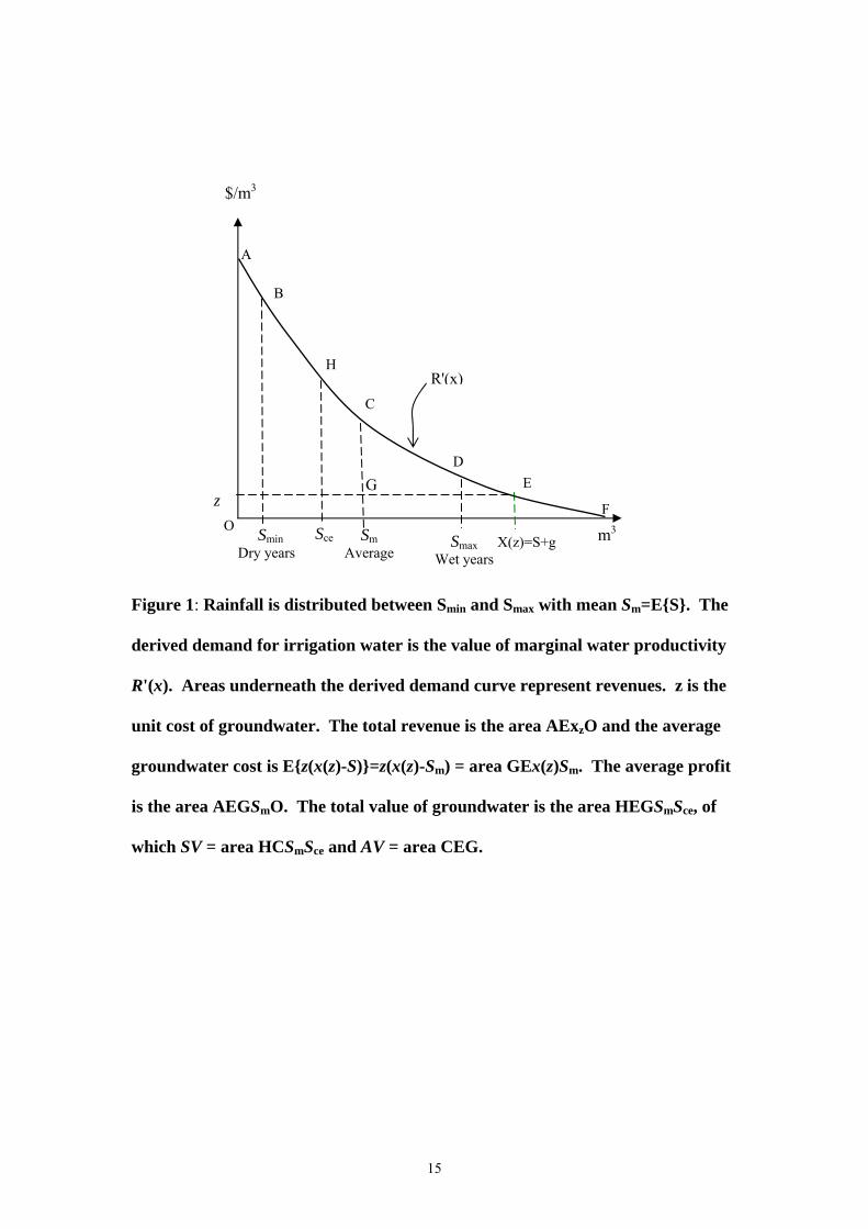
Figure 1: Rainfall is distributed between Smin and Smax with mean Sm=E{S}. The

derived demand for irrigation water is the value of marginal water productivity

R'(x). Areas underneath the derived demand curve represent revenues. z is the

unit cost of groundwater. The total revenue is the area AExzO and the average

groundwater cost is E{z(x(z)-S)}=z(x(z)-Sm) = area GEx(z)Sm. The average profit

is the area AEGSmO. The total value of groundwater is the area HEGSmSce, of

which SV = area HCSmSce and AV = area CEG.

15

0

200

400

600

800

1,000

1,200

1,400

1 3 5 7 9 11 13 15 17 19 21 23 25 27 29

1965-1985, 1991-1999

Figure 2: Annual rainfall (mm) in the Coimbatore District during 1965−1985

and 1991−1999.

16

0

5

1 0

1 5

2 0

2 5

3 0

3 5

4 0

0 1 E + 0 8 2 E + 0 8 3 E + 0 8 4 E + 0 8 5 E + 0 8 6 E + 0 8 7 E + 0 8

m 3

Figure 3: Value of marginal water productivity (Rs m-3) in Coimbatore Water

District.

17

Table 1: Planted area, water requirement, yield and price ($1=48.5 Rs in 2002)

for the 13 main crops of Coimbatore District

Crop Area (hectares)

Water requirement

(m3 ha-1)

Yield (100kg/ha)

Price (R/100kg)

Cotton 8576 6000 2.91 8576 Cholam 6451 3500 0.90 6451

Groundnuts 15145 4500 1.39 15145 Sugarcane 12355 20000 6.49 12355

Chilies 2594 5000 21.76 2594 Tomato 5827 5000.00 13.94 5827

Paddy rice 12258 12500 2.26 12258 Tapioca 1214 6000 32.04 1214

Ragi 80 3500 148.58 80 Turmeric 2910 14000 37.41 2910 Banana 7561 20000 17.99 7561

Soya Beans 35 5000 537.77 35 Onion 2537 3000 45.29 2537

18

Table 2: Per hectare input requirements and costs (Rs ha-1).

Se

eds

Man

ures

Fam

ily m

enla

bor

Fam

ily

wom

en

labo

r H

ired

men

la

bor

Hire

d w

omen

la

bor

Ani

mal

po

wer

M

achi

ne

pow

er

Ferti

lizer

s

Pest

icid

es

Per-

hact

are

cost

(e

xclu

ding

w

ater

)

Cotton 510 778 1730 884 1577 4675 376 1159 1889 1179 14757 Cholam 206 363 661 157 567 562 406 373 212 0 3507 Ground

nuts 3028 767 1328 262 1521 2602 664 638 1006 228 12044

Sugar cane

6224 1206 2649 357 14096 7029 651 5238 4585 581 42616

Chilies 705 1903 2730 800 4000 12423 696 2707 4799 1578 32341 Tomato 173 1750 2669 1086 1717 3586 736 633 1813 824 14987 Paddy

rice 956 1310 1662 282 2503 3582 933 1746 2394 1440 16808

Tapioca 353 1250 4439 1050 4067 4212 240 2783 2281 40 20715 Ragi 136 683 2152 490 974 2458 568 768 1046 20 9295

Turmeric 9206 2095 2702 367 5888 4690 816 725 2686 607 29782 Banana 5525 727 1859 239 19214 4338 210 1963 1266

3 581 47319

Soya Beans

765 276 892 723 698 1365 441 712 1038 217 7127

Onion 7549 3212 5442 769 5497 8578 1319 3794 3783 2985 42928

19

Table 3: Groundwater values (except for last row, all values are in Rs).

Symbol Description Result R(Sm) Revenue at the mean 2,395,063,341 E{R(S)} Mean revenue 2,342,143,999 SV= R(Sm)− E{R(S)} Stabilization Value 52,919,342 R(∞)= Revenue under unlimited water 2,552,096,009 A= R(∞)−R(Sm) Upper bound on Augmentation

Value AV 157,032,667

A + SV Upper bound on the total value of groundwater

209,952,009

SV/(A+SV) Lower bound on share of SV in total value of groundwater

0.252

20

PREVIOUS DISCUSSION PAPERS 1.01 Yoav Kislev - Water Markets (Hebrew). 2.01 Or Goldfarb and Yoav Kislev - Incorporating Uncertainty in Water

Management (Hebrew).

3.01 Zvi Lerman, Yoav Kislev, Alon Kriss and David Biton - Agricultural Output and Productivity in the Former Soviet Republics. 4.01 Jonathan Lipow & Yakir Plessner - The Identification of Enemy Intentions through Observation of Long Lead-Time Military Preparations. 5.01 Csaba Csaki & Zvi Lerman - Land Reform and Farm Restructuring in Moldova: A Real Breakthrough? 6.01 Zvi Lerman - Perspectives on Future Research in Central and Eastern

European Transition Agriculture. 7.01 Zvi Lerman - A Decade of Land Reform and Farm Restructuring: What Russia Can Learn from the World Experience. 8.01 Zvi Lerman - Institutions and Technologies for Subsistence Agriculture: How to Increase Commercialization. 9.01 Yoav Kislev & Evgeniya Vaksin - The Water Economy of Israel--An

Illustrated Review. (Hebrew). 10.01 Csaba Csaki & Zvi Lerman - Land and Farm Structure in Poland. 11.01 Yoav Kislev - The Water Economy of Israel. 12.01 Or Goldfarb and Yoav Kislev - Water Management in Israel: Rules vs. Discretion. 1.02 Or Goldfarb and Yoav Kislev - A Sustainable Salt Regime in the Coastal

Aquifer (Hebrew).

2.02 Aliza Fleischer and Yacov Tsur - Measuring the Recreational Value of Open Spaces. 3.02 Yair Mundlak, Donald F. Larson and Rita Butzer - Determinants of

Agricultural Growth in Thailand, Indonesia and The Philippines. 4.02 Yacov Tsur and Amos Zemel - Growth, Scarcity and R&D. 5.02 Ayal Kimhi - Socio-Economic Determinants of Health and Physical Fitness in Southern Ethiopia. 6.02 Yoav Kislev - Urban Water in Israel. 7.02 Yoav Kislev - A Lecture: Prices of Water in the Time of Desalination.

(Hebrew).

8.02 Yacov Tsur and Amos Zemel - On Knowledge-Based Economic Growth. 9.02 Yacov Tsur and Amos Zemel - Endangered aquifers: Groundwater

management under threats of catastrophic events. 10.02 Uri Shani, Yacov Tsur and Amos Zemel - Optimal Dynamic Irrigation

Schemes. 1.03 Yoav Kislev - The Reform in the Prices of Water for Agriculture (Hebrew). 2.03 Yair Mundlak - Economic growth: Lessons from two centuries of American Agriculture. 3.03 Yoav Kislev - Sub-Optimal Allocation of Fresh Water. (Hebrew). 4.03 Dirk J. Bezemer & Zvi Lerman - Rural Livelihoods in Armenia. 5.03 Catherine Benjamin and Ayal Kimhi - Farm Work, Off-Farm Work, and Hired Farm Labor: Estimating a Discrete-Choice Model of French Farm Couples' Labor Decisions. 6.03 Eli Feinerman, Israel Finkelshtain and Iddo Kan - On a Political Solution to the Nimby Conflict. 7.03 Arthur Fishman and Avi Simhon - Can Income Equality Increase

Competitiveness? 8.03 Zvika Neeman, Daniele Paserman and Avi Simhon - Corruption and

Openness. 9.03 Eric D. Gould, Omer Moav and Avi Simhon - The Mystery of Monogamy. 10.03 Ayal Kimhi - Plot Size and Maize Productivity in Zambia: The Inverse Relationship Re-examined. 11.03 Zvi Lerman and Ivan Stanchin - New Contract Arrangements in Turkmen Agriculture: Impacts on Productivity and Rural Incomes. 12.03 Yoav Kislev and Evgeniya Vaksin - Statistical Atlas of Agriculture in Israel - 2003-Update (Hebrew). 1.04 Sanjaya DeSilva, Robert E. Evenson, Ayal Kimhi - Labor Supervision and Transaction Costs: Evidence from Bicol Rice Farms. 2.04 Ayal Kimhi - Economic Well-Being in Rural Communities in Israel. 3.04 Ayal Kimhi - The Role of Agriculture in Rural Well-Being in Israel. 4.04 Ayal Kimhi - Gender Differences in Health and Nutrition in Southern Ethiopia. 5.04 Aliza Fleischer and Yacov Tsur - The Amenity Value of Agricultural Landscape and Rural-Urban Land Allocation.

6.04 Yacov Tsur and Amos Zemel – Resource Exploitation, Biodiversity and Ecological Events.

7.04 Yacov Tsur and Amos Zemel – Knowledge Spillover, Learning Incentives

And Economic Growth. 8.04 Ayal Kimhi – Growth, Inequality and Labor Markets in LDCs: A Survey. 9.04 Ayal Kimhi – Gender and Intrahousehold Food Allocation in Southern

Ethiopia 10.04 Yael Kachel, Yoav Kislev & Israel Finkelshtain – Equilibrium Contracts in

The Israeli Citrus Industry.

11.04 Zvi Lerman, Csaba Csaki & Gershon Feder – Evolving Farm Structures and Land Use Patterns in Former Socialist Countries. 12.04 Margarita Grazhdaninova and Zvi Lerman – Allocative and Technical Efficiency of Corporate Farms. 13.04 Ruerd Ruben and Zvi Lerman – Why Nicaraguan Peasants Stay in

Agricultural Production Cooperatives.

14.04 William M. Liefert, Zvi Lerman, Bruce Gardner and Eugenia Serova - Agricultural Labor in Russia: Efficiency and Profitability. 1.05 Yacov Tsur and Amos Zemel – Resource Exploitation, Biodiversity Loss

and Ecological Events. 2.05 Zvi Lerman and Natalya Shagaida – Land Reform and Development of

Agricultural Land Markets in Russia.

3.05 Ziv Bar-Shira, Israel Finkelshtain and Avi Simhon – Regulating Irrigation via Block-Rate Pricing: An Econometric Analysis.

4.05 Yacov Tsur and Amos Zemel – Welfare Measurement under Threats of

Environmental Catastrophes. 5.05 Avner Ahituv and Ayal Kimhi – The Joint Dynamics of Off-Farm

Employment and the Level of Farm Activity. 6.05 Aliza Fleischer and Marcelo Sternberg – The Economic Impact of Global

Climate Change on Mediterranean Rangeland Ecosystems: A Space-for-Time Approach.

7.05 Yael Kachel and Israel Finkelshtain – Antitrust in the Agricultural Sector:

A Comparative Review of Legislation in Israel, the United States and the European Union.

8.05 Zvi Lerman – Farm Fragmentation and Productivity Evidence from Georgia. 9.05 Zvi Lerman – The Impact of Land Reform on Rural Household Incomes in

Transcaucasia and Central Asia.

10.05 Zvi Lerman and Dragos Cimpoies – Land Consolidation as a Factor for Successful Development of Agriculture in Moldova. 11.05 Rimma Glukhikh, Zvi Lerman and Moshe Schwartz – Vulnerability and Risk

Management among Turkmen Leaseholders. 12.05 R.Glukhikh, M. Schwartz, and Z. Lerman – Turkmenistan’s New Private

Farmers: The Effect of Human Capital on Performance. 13.05 Ayal Kimhi and Hila Rekah – The Simultaneous Evolution of Farm Size and

Specialization: Dynamic Panel Data Evidence from Israeli Farm Communities.

14.05 Jonathan Lipow and Yakir Plessner - Death (Machines) and Taxes. 1.06 Yacov Tsur and Amos Zemel – Regulating Environmental Threats. 2.06 Yacov Tsur and Amos Zemel - Endogenous Recombinant Growth. 3.06 Yuval Dolev and Ayal Kimhi – Survival and Growth of Family Farms in

Israel: 1971-1995. 4.06 Saul Lach, Yaacov Ritov and Avi Simhon – Longevity across Generations. 5.06 Anat Tchetchik, Aliza Fleischer and Israel Finkelshtain – Differentiation &

Synergies in Rural Tourism: Evidence from Israel.

6.06 Israel Finkelshtain and Yael Kachel – The Organization of Agricultural Exports: Lessons from Reforms in Israel.

7.06 Zvi Lerman, David Sedik, Nikolai Pugachev and Aleksandr Goncharuk –

Ukraine after 2000: A Fundamental Change in Land and Farm Policy?

8.06 Zvi Lerman and William R. Sutton – Productivity and Efficiency of Small and Large Farms in Moldova.

9.06 Bruce Gardner and Zvi Lerman – Agricultural Cooperative Enterprise in

the Transition from Socialist Collective Farming. 10.06 Zvi Lerman and Dragos Cimpoies - Duality of Farm Structure in

Transition Agriculture: The Case of Moldova. 11.06 Yael Kachel and Israel Finkelshtain – Economic Analysis of Cooperation

In Fish Marketing. (Hebrew) 12.06 Anat Tchetchik, Aliza Fleischer and Israel Finkelshtain – Rural Tourism:

Developmelnt, Public Intervention and Lessons from the Israeli Experience.

13.06 Gregory Brock, Margarita Grazhdaninova, Zvi Lerman, and Vasilii Uzun - Technical Efficiency in Russian Agriculture.

14.06 Amir Heiman and Oded Lowengart - Ostrich or a Leopard – Communication

Response Strategies to Post-Exposure of Negative Information about Health Hazards in Foods

15.06 Ayal Kimhi and Ofir D. Rubin – Assessing the Response of Farm Households to Dairy Policy Reform in Israel. 16.06 Iddo Kan, Ayal Kimhi and Zvi Lerman – Farm Output, Non-Farm Income, and

Commercialization in Rural Georgia. 1.07 Joseph Gogodze, Iddo Kan and Ayal Kimhi – Land Reform and Rural Well

Being in the Republic of Georgia: 1996-2003. 2.07 Uri Shani, Yacov Tsur, Amos Zemel & David Zilberman – Irrigation Production

Functions with Water-Capital Substitution. 3.07 Masahiko Gemma and Yacov Tsur – The Stabilization Value of Groundwater

and Conjunctive Water Management under Uncertainty.