Management Science – MNG221

Lecture 1: Transportation, Transshipment, and Assignment

Transportation, Transshipment, and Assignment

• Transportation, transshipment, and assignment problems are special types of linear programming model formulations.• They are part of a larger class of linear

programming problems known as network flow problems.• There solution approaches are variations of

the traditional simplex solution procedure.

Transportation ModelTransportation, Transshipment, and Assignment

Transportation Model

• Transportation models are formulated to solve problems where:A product is transported from a number of

sources to a number of destinations at the minimum possible cost.

Each source is able to supply a fixed number of units of the product, and each destination has a fixed demand for the product.

Transportation Model

• In a transportation problem, items are allocated from sources to destinations at a minimum cost.• The linear programming model for a

transportation problem has constraints for supply at each source and demand at each destination.

Transportation Model• A Transportation can be a:

1. Balanced transportation model in which supply equals demand, all constraints are equalities. Supply = Demand

2. Unbalanced transportation model in which supply exceeds demand or demand exceeds supply:Supply < Demand

Supply > DemandTransportation problems are usually solved manually within a tableau format.

The Transshipment ModelTransportation, Transshipment, and Assignment

Transshipment Model

• The transshipment model is an extension of the transportation model in which intermediate transshipment points are added between the sources and destinations.

• An example of a transshipment point is a distribution center or warehouse located between plants and stores.

Transshipment Model

• In a transshipment problem, items may be transported:1. From sources through transshipment

points on to destinations, 2. From one source to another,3. From one transshipment point to

another,

Transshipment Model

4. From one destination to another, 5. Or directly from sources to

destinations, 6. Or some combination of these

alternatives.• The transshipment model includes

intermediate points between sources and destinations.

The Assignment ModelTransportation, Transshipment, and Assignment

Assignment Model

• The Assignment Model is a special form of a linear programming model that is similar to the transportation model.

• The differences, however, is that the supply at each source and the demand at each destination are each limited to one unit.

Assignment Model

• The linear programming formulation of the assignment model is similar to the formulation of the transportation model, except all the supply values for each source equal one, and all the demand values at each destination equal one.

Transportation: Worked ExampleTransportation, Transshipment, and Assignment

Transportation: Worked Example

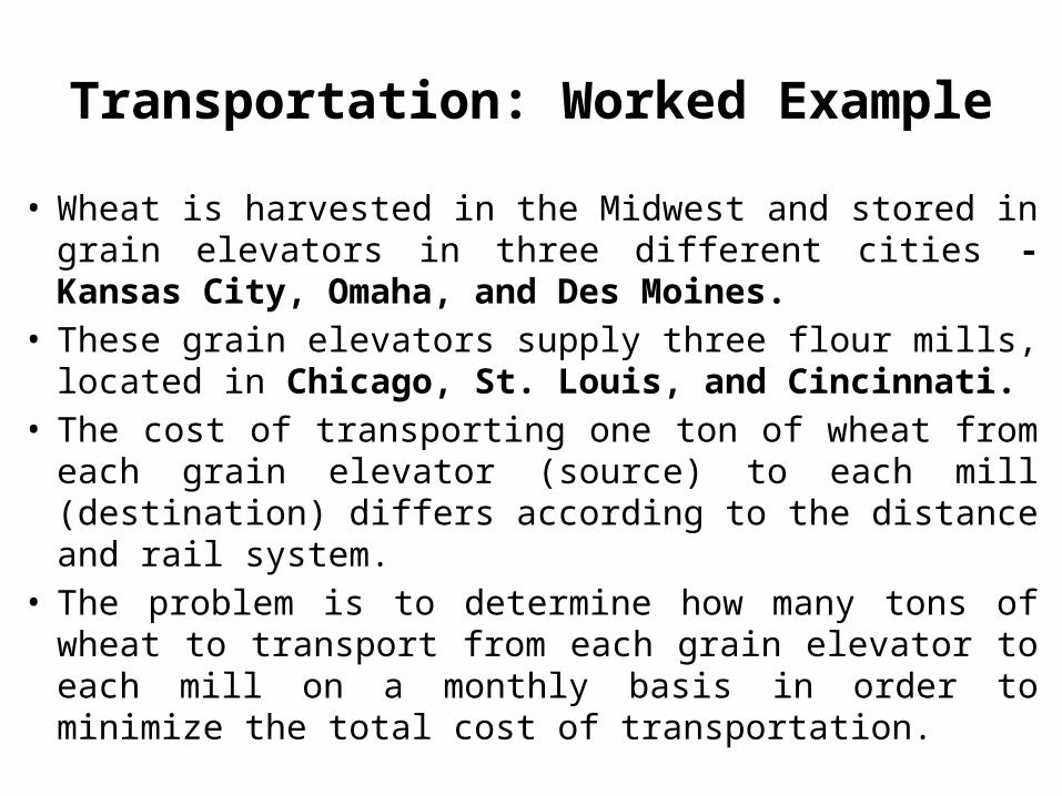
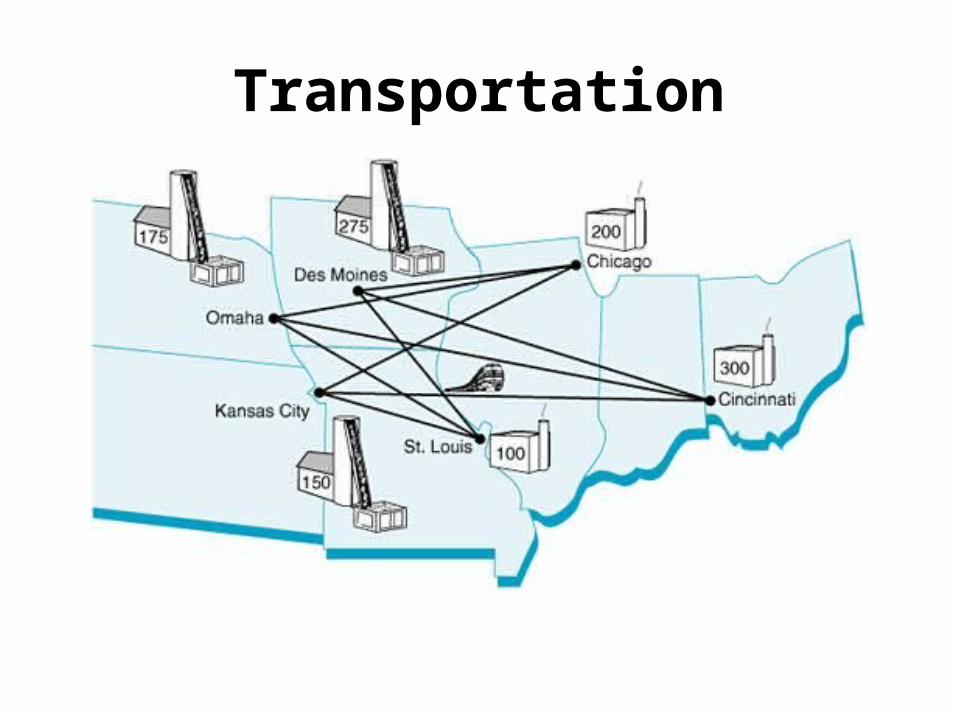
• Wheat is harvested in the Midwest and stored in grain elevators in three different cities - Kansas City, Omaha, and Des Moines.

• These grain elevators supply three flour mills, located in Chicago, St. Louis, and Cincinnati.

• The cost of transporting one ton of wheat from each grain elevator (source) to each mill (destination) differs according to the distance and rail system.

• The problem is to determine how many tons of wheat to transport from each grain elevator to each mill on a monthly basis in order to minimize the total cost of transportation.

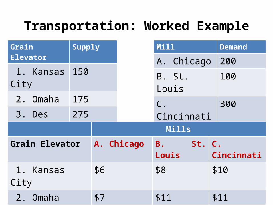
Transportation: Worked ExampleGrain Elevator Supply

1. Kansas City 150

2. Omaha 175

3. Des Moines 275

Total 600

Mill Demand

A. Chicago 200

B. St. Louis 100

C. Cincinnati 300

Total 600

Mills

Grain Elevator A. Chicago B. St. Louis C. Cincinnati

1. Kansas City $6 $8 $10

2. Omaha $7 $11 $11

3. Des Moines $4 $5 $12

Transportation: Worked ExampleTransportation, Transshipment, and Assignment

Transportation

Transportation: Worked ExampleGrain Elevator Supply

1. Kansas City 150

2. Omaha 175

3. Des Moines 275

Total 600

Mill Demand

A. Chicago 200

B. St. Louis 100

C. Cincinnati 300

Total 600

Mills

Grain Elevator A. Chicago B. St. Louis C. Cincinnati

1. Kansas City $6 $8 $10

2. Omaha $7 $11 $11

3. Des Moines $4 $5 $12

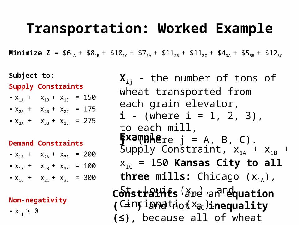
Transportation: Worked ExampleMinimize Z = $61A + $81B + $101C + $72A + $112B + $112C + $43A + $53B + $123C

Subject to:Supply Constraints• x1A + x1B + x1C = 150

• x2A + x2B + x2C = 175

• x3A + x3B + x3C = 275

Demand Constraints• x1A + x2A + x3A = 200

• x1B + x2B + x3B = 100

• x1C + x2C + x3C = 300

Non-negativity• xij ≥ 0

Xij - the number of tons of wheat transported from each grain elevator, i - (where i = 1, 2, 3), to each mill, j -(where j = A, B, C).

Example Supply Constraint, x1A + x1B + x1C = 150 Kansas City to all three mills: Chicago (x1A), St. Louis (x1B), and Cincinnati (x1C).

Constraints are an equation ( = ) and not a inequality (≤), because all of wheat available is needed to meet demand of 600 tons.

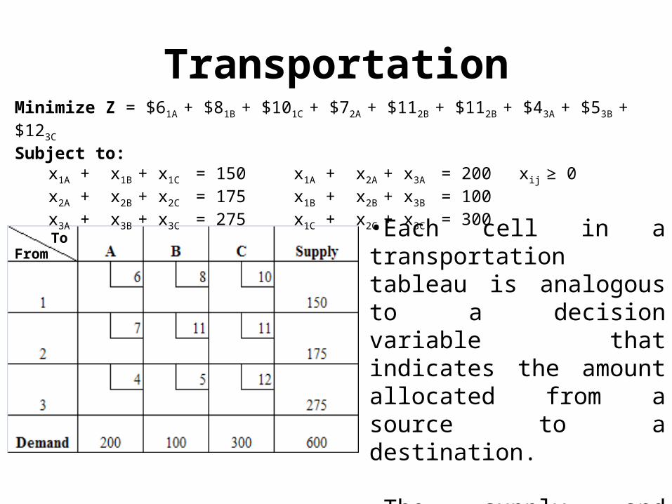
TransportationMinimize Z = $61A + $81B + $101C + $72A + $112B + $112B + $43A + $53B + $123C

Subject to:x1A + x1B + x1C = 150 x1A + x2A + x3A = 200 xij ≥ 0x2A + x2B + x2C = 175 x1B + x2B + x3B = 100 x3A + x3B + x3C = 275 x1C + x2C + x3C = 300

•Each cell in a transportation tableau is analogous to a decision variable that indicates the amount allocated from a source to a destination.

•The supply and demand values along the outside of the rim of the tableau are called rim requirements.

FromTo

Transportation: Worked Example

• 2 -Methods for solving a Transportation Model –1. The Stepping-Stone Method 2. The Modified Distribution Method (also known

as MODI)

BUT

• Must be given an Initial Solution1. The Northwest Corner Method2. The Minimum Cell Cost Method3. Vogel’s Approximation Method

TransportationFrom

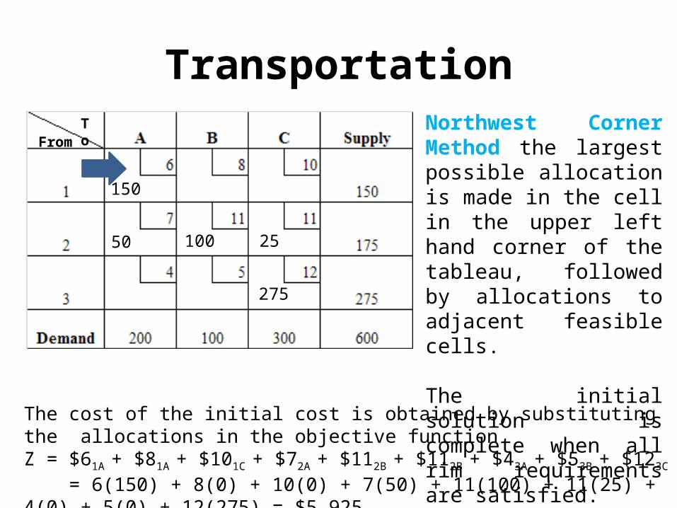
To Northwest Corner Method the largest possible allocation is made in the cell in the upper left hand corner of the tableau, followed by allocations to adjacent feasible cells.

The initial solution is complete when all rim requirements are satisfied.

150

50 100 25

275

The cost of the initial cost is obtained by substituting the allocations in the objective functionZ = $61A + $81A + $101C + $72A + $112B + $112B + $43A + $53B + $123C

= 6(150) + 8(0) + 10(0) + 7(50) + 11(100) + 11(25) + 4(0) + 5(0) + 12(275) = $5,925

TransportationFrom

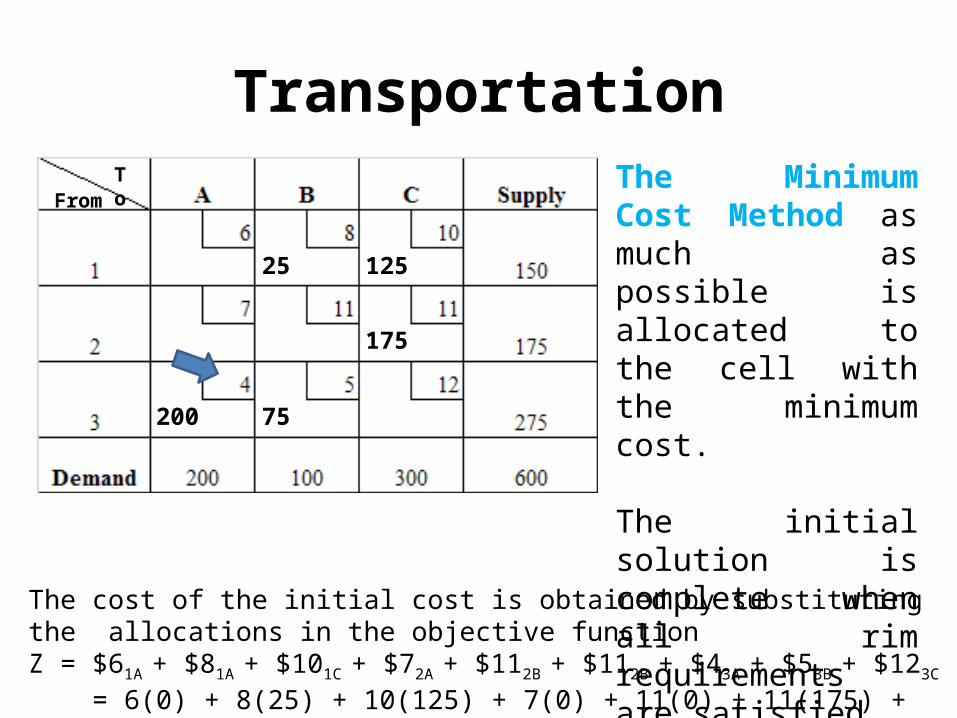
To The Minimum Cost Method as much as possible is allocated to the cell with the minimum cost.

The initial solution is complete when all rim requirements are satisfied.

200 75

25 125

175

The cost of the initial cost is obtained by substituting the allocations in the objective functionZ = $61A + $81A + $101C + $72A + $112B + $112B + $43A + $53B + $123C

= 6(0) + 8(25) + 10(125) + 7(0) + 11(0) + 11(175) + 4(200) + 5(75) + 12(0) = $4,550

Transportation

• Vogel's Approximation Model is based on the concept of penalty cost or regret.

• A Penalty Cost is the difference between the largest and next largest cell cost in a row (or column).

• VAM allocates as much as possible to the minimum cost cell in the row or column with the largest penalty cost.

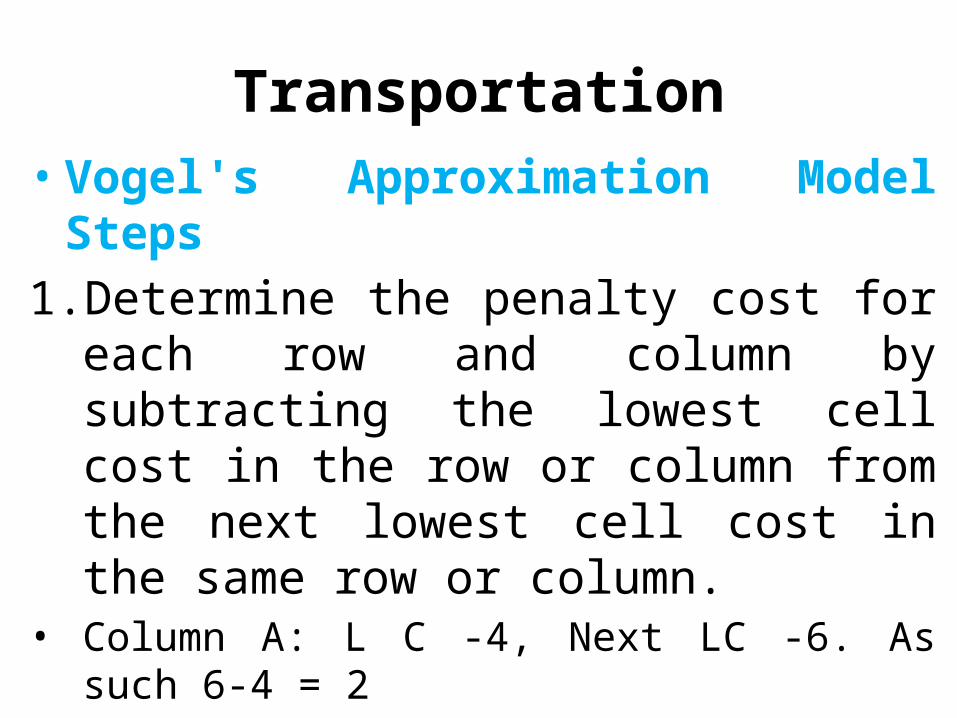
Transportation• Vogel's Approximation Model Steps1. Determine the penalty cost for each row and

column by subtracting the lowest cell cost in the row or column from the next lowest cell cost in the same row or column.

• Column A: L C -4, Next LC -6. As such 6-4 = 2

2. Select the row or column with the highest penalty cost (breaking ties arbitrarily or choosing the lowest-cost cell).

Transportation

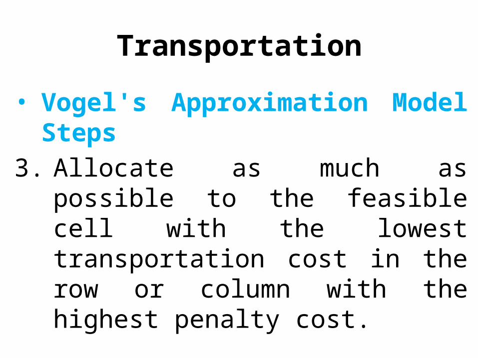
• Vogel's Approximation Model Steps3. Allocate as much as possible to the

feasible cell with the lowest transportation cost in the row or column with the highest penalty cost.

4. Repeat steps 1, 2, and 3 until all rim requirements have been met.

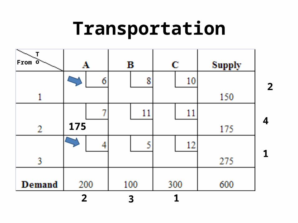
TransportationFrom

To

2 3

2

1

4

1

175

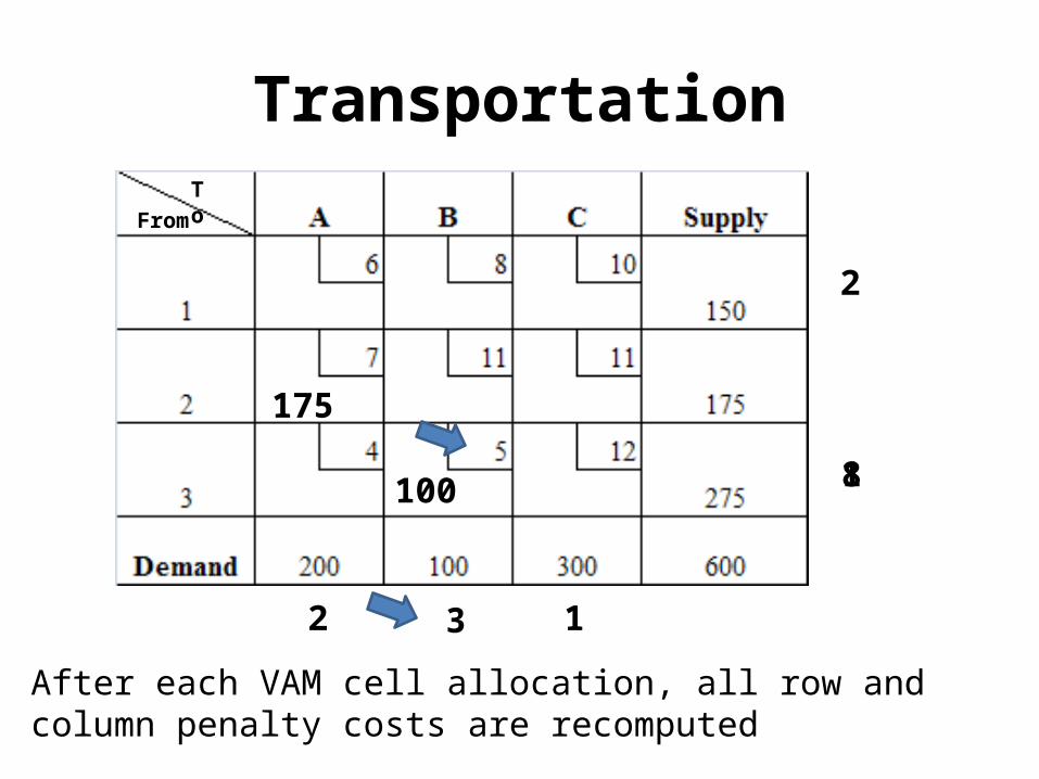
Transportation

FromTo

2 3

2

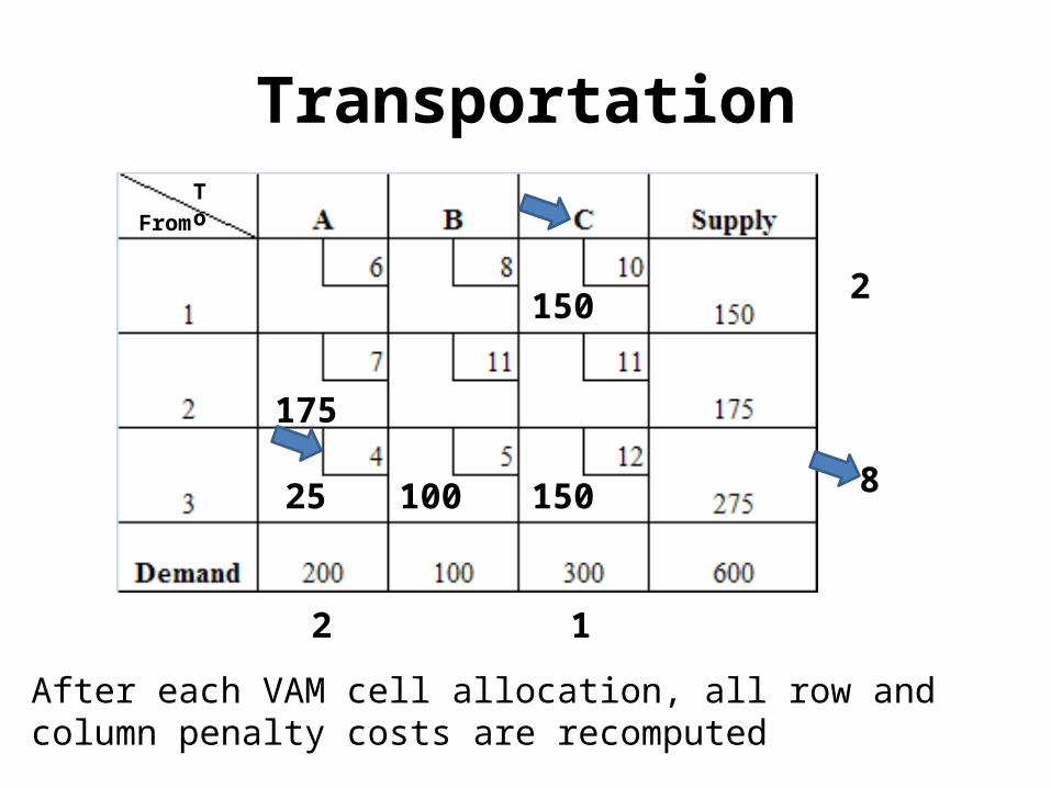
After each VAM cell allocation, all row and column penalty costs are recomputed

1

1

175

100 8

Transportation

FromTo

2

2

After each VAM cell allocation, all row and column penalty costs are recomputed

1

175

100 825 150

150

Transportation

FromTo

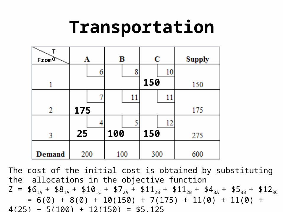
The cost of the initial cost is obtained by substituting the allocations in the objective functionZ = $61A + $81A + $101C + $72A + $112B + $112B + $43A + $53B + $123C

= 6(0) + 8(0) + 10(150) + 7(175) + 11(0) + 11(0) + 4(25) + 5(100) + 12(150) = $5,125

175

10025 150

150

Transportation

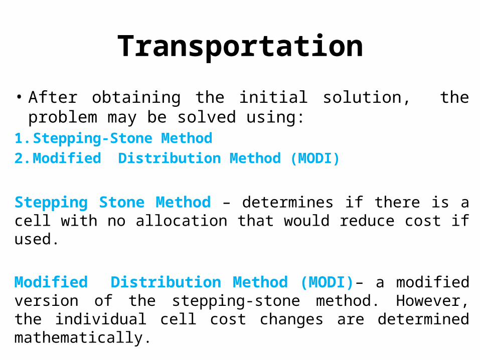
• After obtaining the initial solution, the problem may be solved using:

1. Stepping-Stone Method2. Modified Distribution Method (MODI)

Stepping Stone Method – determines if there is a cell with no allocation that would reduce cost if used.

Modified Distribution Method (MODI)– a modified version of the stepping-stone method. However, the individual cell cost changes are determined mathematically.

Transportation

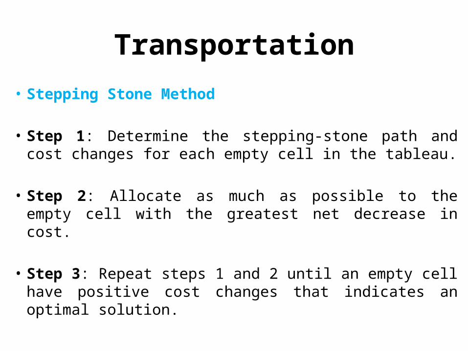
• Stepping Stone Method

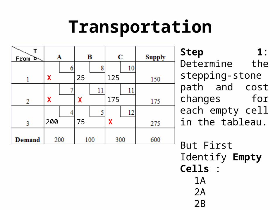
• Step 1: Determine the stepping-stone path and cost changes for each empty cell in the tableau.

• Step 2: Allocate as much as possible to the empty cell with the greatest net decrease in cost.

• Step 3: Repeat steps 1 and 2 until an empty cell have positive cost changes that indicates an optimal solution.

TransportationFrom

To Step 1: Determine the stepping-stone path and cost changes for each empty cell in the tableau.

But First Identify Empty Cells :

1A2A2B3C

200 75

25 125

175

X

X X

X

TransportationFrom

To Evaluation of Cell1A

In evaluating the empty cells the constraint of the problems cannot be violated, and feasibility must be maintained.

Review of the cost increase/reduction of the process.

$6 - $8 + $5 - $4 = -$1

200 75

25 125

175

+1

-1 +1

-1

1A 1B 3B 3A

TransportationFrom

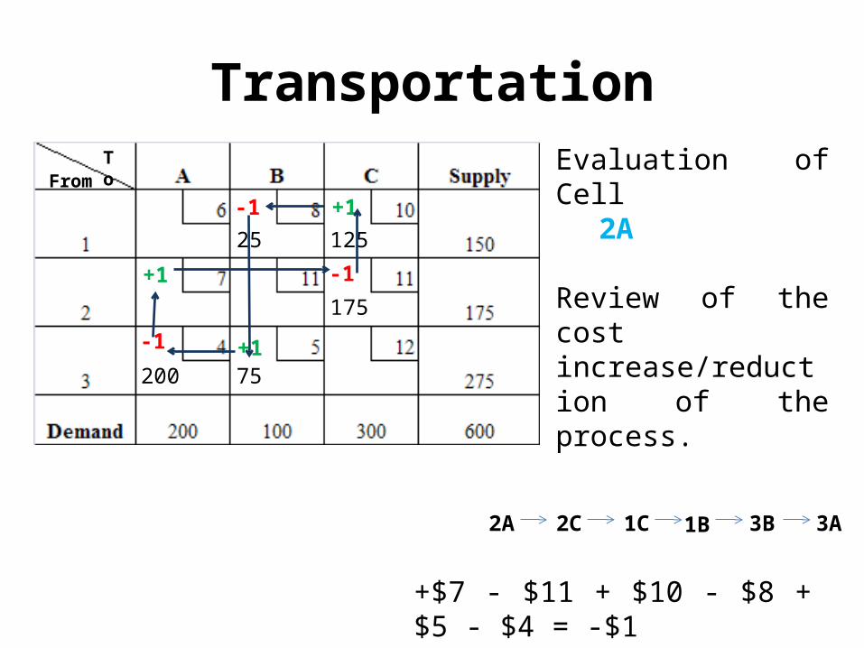
To Evaluation of Cell2A

Review of the cost increase/reduction of the process.

200 75

25 125

175+1

-1 +1

-1

2A 2C 1C 1B

-1 +1

3B 3A

+$7 - $11 + $10 - $8 +$5 - $4 = -$1

TransportationFrom

To Evaluation of Cell1A2A2B3C

Review of the cost increase/reduction of the process.

+$11 - $11 + $10 - $8 = +$2

200 75

25 125

175+1

-1 +1

-1

2B 2C 1C 1B

TransportationFrom

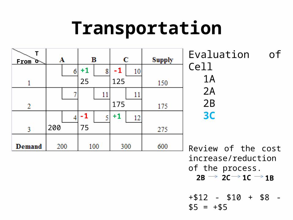
To Evaluation of Cell1A2A2B3C

Review of the cost increase/reduction of the process.

+$12 - $10 + $8 - $5 = +$5

200 75

25 125

175

+1

-1+1

-1

2B 2C 1C 1B

TransportationFrom

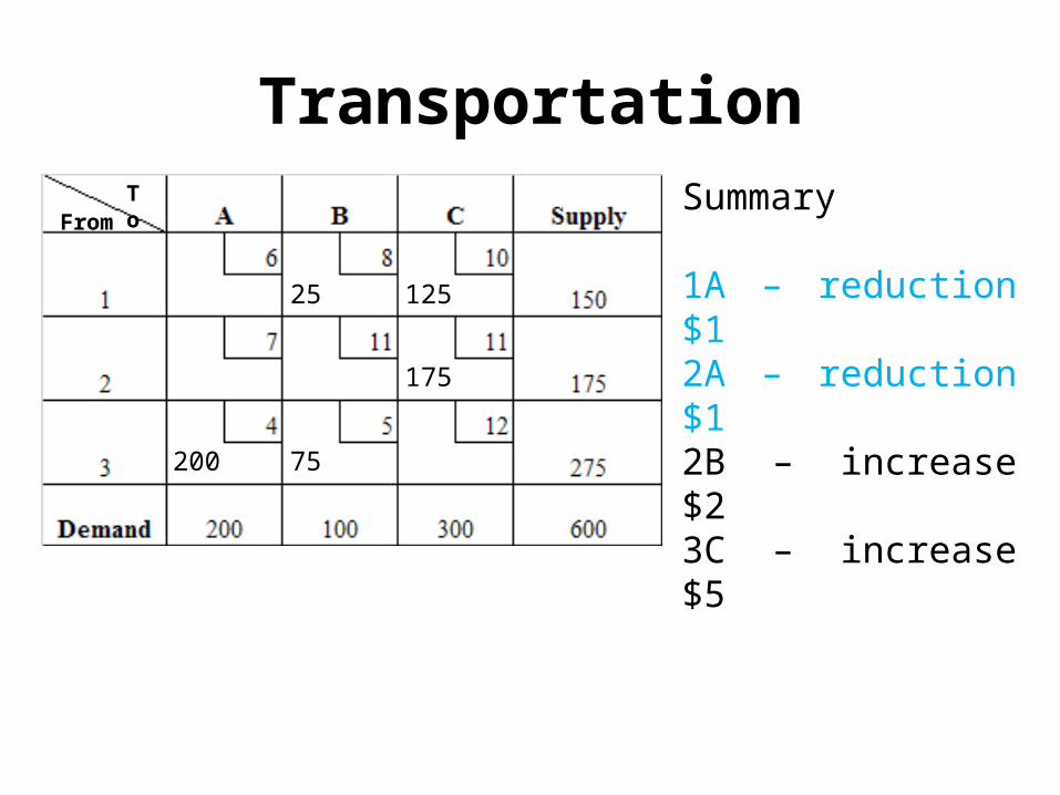
To Summary

1A – reduction $12A – reduction $12B – increase $23C – increase $5

200 75

25 125

175

TransportationFrom

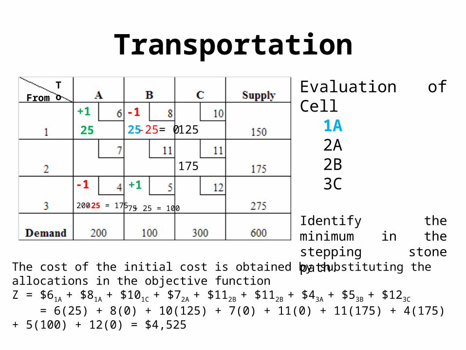
To Evaluation of Cell1A2A2B3C

Identify the minimum in the stepping stone path.

200 75

25 125

175

+1

-1 +1

-1-25= 025

-25 = 175 + 25 = 100

The cost of the initial cost is obtained by substituting the allocations in the objective functionZ = $61A + $81A + $101C + $72A + $112B + $112B + $43A + $53B + $123C

= 6(25) + 8(0) + 10(125) + 7(0) + 11(0) + 11(175) + 4(175) + 5(100) + 12(0) = $4,525

The Assignment ModelTransportation, Transshipment, and Assignment

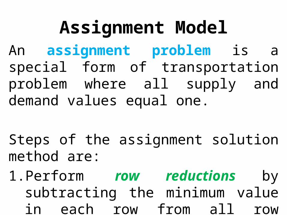
Assignment ModelAn assignment problem is a special form of transportation problem where all supply and demand values equal one.

Steps of the assignment solution method are:1. Perform row reductions by subtracting the

minimum value in each row from all row values.

Assignment ModelSteps of the assignment solution method (Continued)2. Perform column reductions by subtracting

the minimum value in each column from all column value.

3. In the completed Opportunity Cost Table, cross out all zeros, using the minimum number of horizontal or vertical lines.

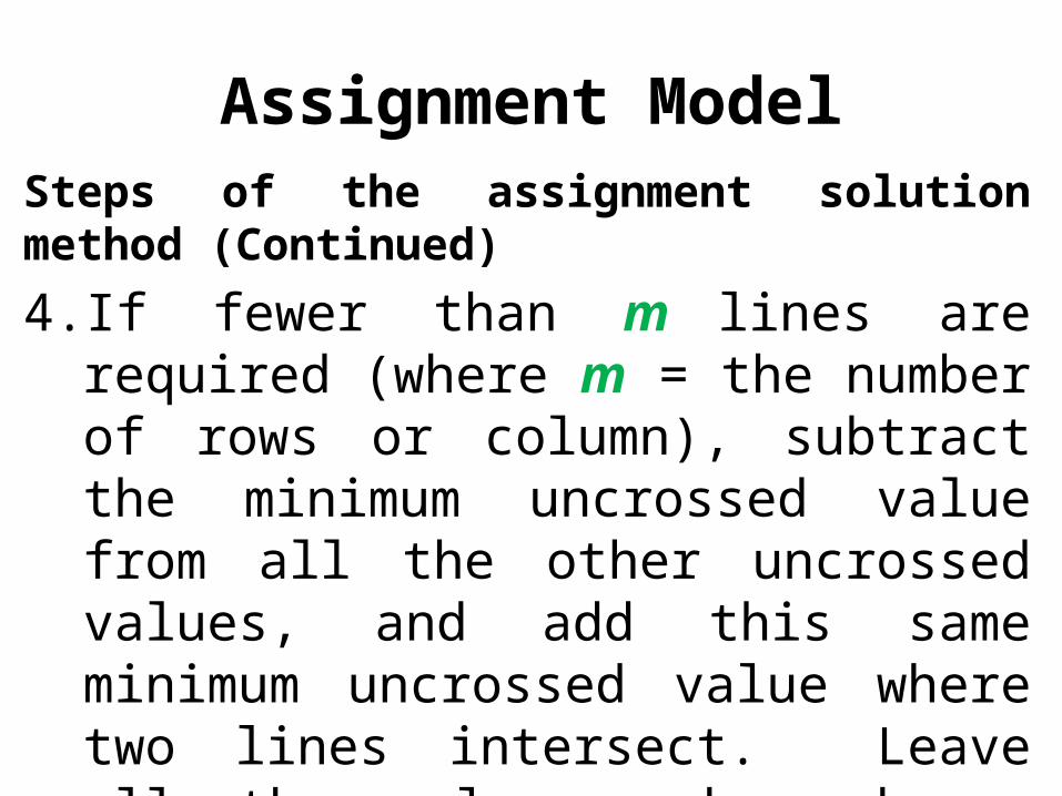
Assignment ModelSteps of the assignment solution method (Continued)4. If fewer than m lines are required (where m

= the number of rows or column), subtract the minimum uncrossed value from all the other uncrossed values, and add this same minimum uncrossed value where two lines intersect. Leave all other values unchanged.

Assignment ModelSteps of the assignment solution method (Continued)5. If m lines are required, the tableau contains

the optimal solution and m unique assignments are made. If fewer than m lines are required, repeat step 4.

The Assignment Model- A Worked Example

Transportation, Transshipment, and Assignment

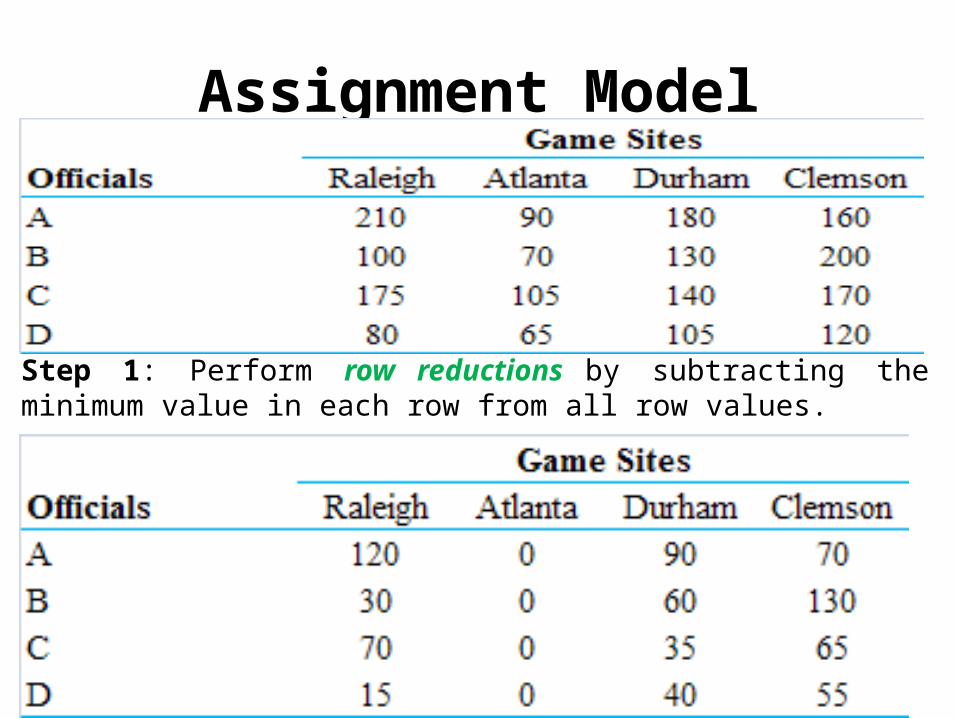
Assignment Model - Example• The Atlantic Coast Conference has four

basketball games on a particular night.

• The conference office wants to assign four teams of officials to the four games in a way that will minimize the total distance traveled by the officials.

• The distances in miles for each team of officials to each game location are shown below.

Assignment Model

Step 1: Perform row reductions by subtracting the minimum value in each row from all row values.

Assignment Model

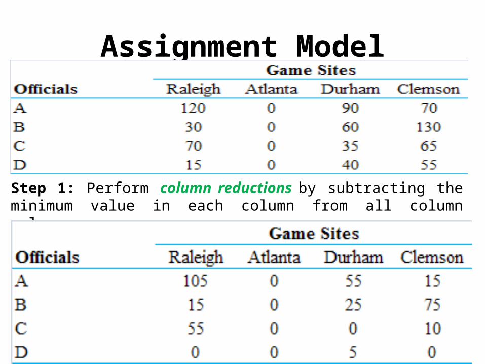
Step 1: Perform column reductions by subtracting the minimum value in each column from all column value.

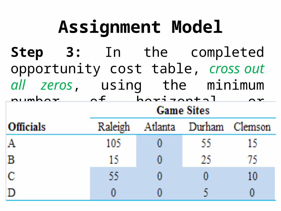
Assignment ModelStep 3: In the completed opportunity cost table, cross out all zeros, using the minimum number of horizontal or vertical lines.

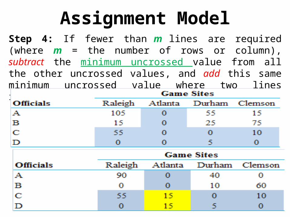
Assignment ModelStep 4: If fewer than m lines are required (where m = the number of rows or column), subtract the minimum uncrossed value from all the other uncrossed values, and add this same minimum uncrossed value where two lines intersect. Leave all other values unchanged.

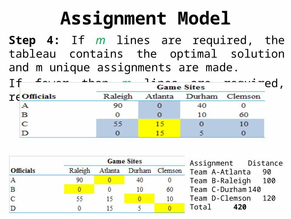
Assignment ModelStep 4: If m lines are required, the tableau contains the optimal solution and m unique assignments are made. If fewer than m lines are required, repeat step 4.

Assignment DistanceTeam A-Atlanta 90Team B-Raleigh 100Team C-Durham 140Team D-Clemson 120Total 420

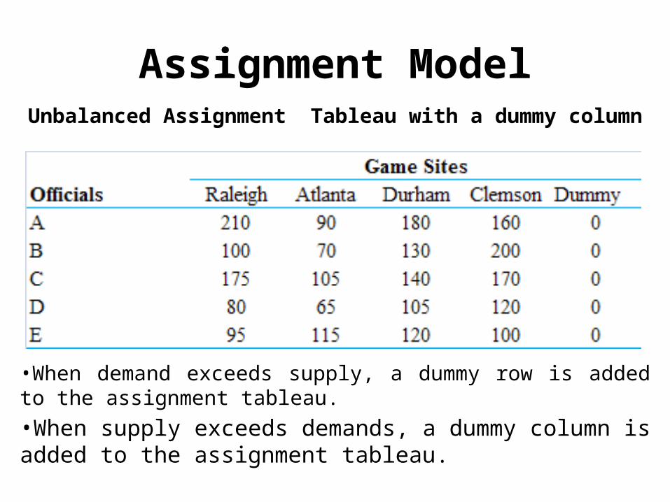
Assignment ModelUnbalanced Assignment Tableau with a dummy column

•When demand exceeds supply, a dummy row is added to the assignment tableau.•When supply exceeds demands, a dummy column is added to the assignment tableau.