Embed Size (px)
Citation preview

Management strategy evaluation for the Gulf of Alaska walleye pollock fishery: how persistent are the environmental-recruitment links?
Teresa A’marAlaska Fisheries Science Center19 May 2012

The MSE framework
Biological System Exploitation System
Operating model – “true” state
Stock assessment Management actions
Management strategy – perceived state
From Fromentin and Kell, 2007
Observations Implementation
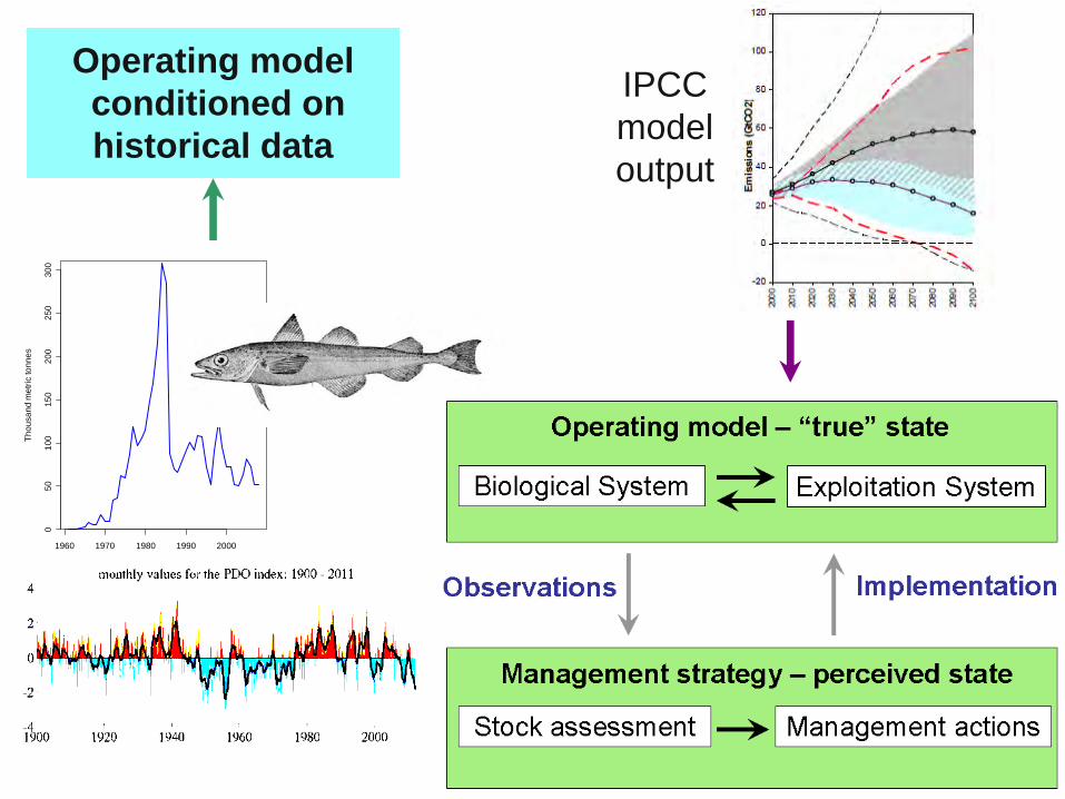
Operating modelconditioned onhistorical data
1960 1970 1980 1990 2000
050
100
150
200
250
300
Year
Thou
sand
met
ric to
nnes
IPCCmodeloutput
1960 1970 1980 1990 2000 2010
0e+0
02e
+09
4e+0
96e
+09
8e+0
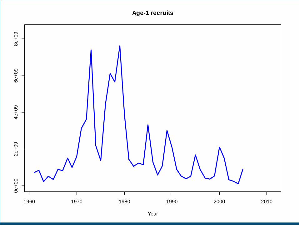
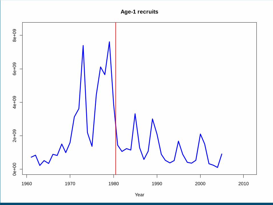
9Age-1 recruits
Year
1960 1970 1980 1990 2000 2010
0e+0
02e
+09
4e+0
96e
+09
8e+0
9Age-1 recruits
Year
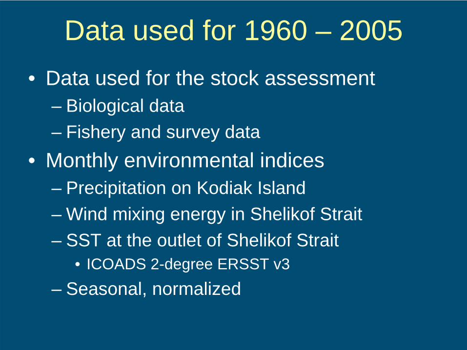
Data used for 1960 – 2005• Data used for the stock assessment
– Biological data– Fishery and survey data
• Monthly environmental indices– Precipitation on Kodiak Island– Wind mixing energy in Shelikof Strait– SST at the outlet of Shelikof Strait
• ICOADS 2-degree ERSST v3– Seasonal, normalized

Winter precipitation - positiveSummer precipitation - negativeSpring SST - negativeSummer SST - positiveAutumn SST – negative
Projected through 2050 with IPCC A1B
1 1 ,ln( ) lny j j y yj
R R a Index ε+ = + +∑Estimated within the model

Projected age-1 recruits
2010 2020 2030 2040 2050
02
46
810
ccsm31
Year
Rec
ruits
(in
billio
ns)
2010 2020 2030 2040 2050
02
46
810
gfdl201
Year
Rec
ruits
(in
billio
ns)
2010 2020 2030 2040 2050
02
46
810
gfdl211
Year
Rec
ruits
(in
billio
ns)
2010 2020 2030 2040 2050
02
46
810
mirocH1
Year
Rec
ruits
(in
billio
ns)
2010 2020 2030 2040 2050
02
46
810
mirocM1
Year
Rec
ruits
(in
billio
ns)
2010 2020 2030 2040 2050
02
46
810
mirocM2
Year
Rec
ruits
(in
billio
ns)
2010 2020 2030 2040 2050
02
46
810
mirocM3
Year
Rec
ruits
(in
billio
ns)
2010 2020 2030 2040 2050
02
46
810
ukhadcm31
YearR
ecru
its (i
n bi
llions
)
Alternative approach
Simple linear models independentof the population dynamics model
1960 1970 1980 1990 2000
1920
2122
1960 on - OM 1 indices
ln(A
ge-1
recr
uits
)
1985 1990 1995 2000 2005
18.5
19.0
19.5
20.0
20.5
21.0
21.5
22.0
1980 on - OM 1 indices
ln(A
ge-1
recr
uits
)
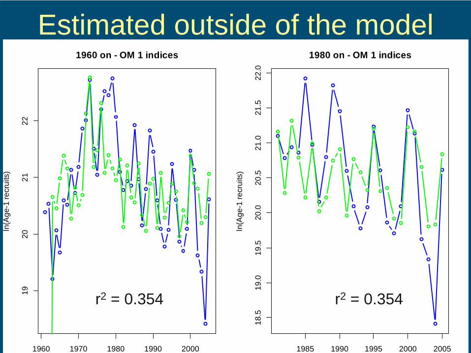
Estimated outside of the model
r2 = 0.354 r2 = 0.354
1960 1970 1980 1990 2000
1920
2122
1960 on - all precip (w/o Spr) and SST
ln(A
ge-1
recr
uits
)
1985 1990 1995 2000 2005
18.5
19.0
19.5
20.0
20.5
21.0
21.5
22.0
1980 on - all precip (w/o Spr) and SST
ln(A
ge-1
recr
uits
)
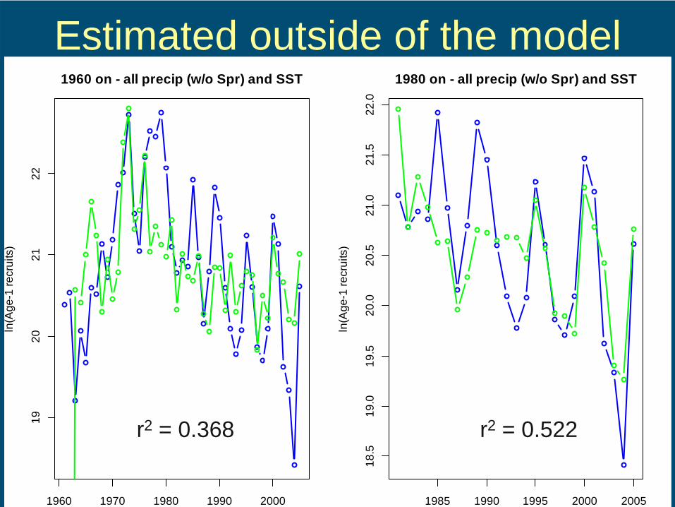
Estimated outside of the model
r2 = 0.368 r2 = 0.522

Summary with 2005 data• Previous model
– Winter precipitation - positive– Summer precipitation - negative– Spring SST - negative– Summer SST - positive– Autumn SST - negative
• New model includes– Autumn precipitation - negative– Winter SST - negative

Current results
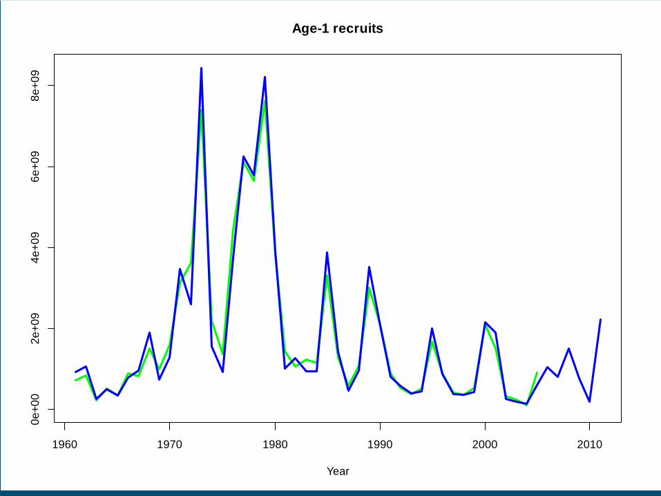
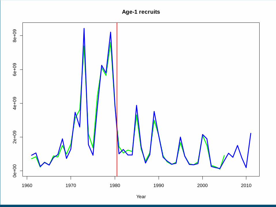
1960 1970 1980 1990 2000 2010
0e+0
02e
+09
4e+0
96e
+09
8e+0
9Age-1 recruits
Year
1960 1970 1980 1990 2000 2010
0e+0
02e
+09
4e+0
96e
+09
8e+0
9Age-1 recruits
Year
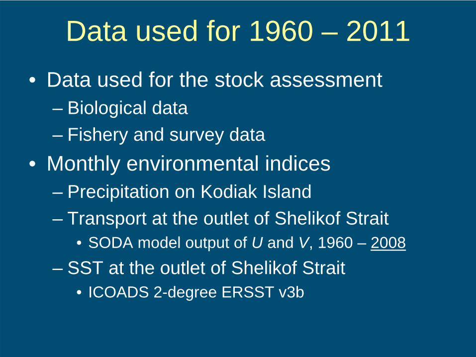
Data used for 1960 – 2011• Data used for the stock assessment
– Biological data– Fishery and survey data
• Monthly environmental indices– Precipitation on Kodiak Island– Transport at the outlet of Shelikof Strait
• SODA model output of U and V, 1960 – 2008– SST at the outlet of Shelikof Strait
• ICOADS 2-degree ERSST v3b

0.45
0.5
0.55
0.6
0.65
0.7
0.75
0.8
0.85
0.9
0.95
1
Jan
Feb
Mar
Apr
May
June July
Aug
Sep
t
Oct
Nov
Dec
Previous vs. current SST data
Correlation with previous SST datafor 1960 – 2005, by month
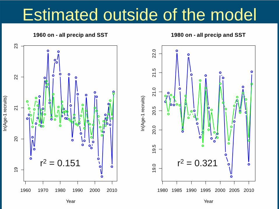
1960 1970 1980 1990 2000 2010
1920
2122
23
1960 on - all precip and SST
Year
ln(A
ge-1
recr
uits
)
1980 1985 1990 1995 2000 2005 2010
19.0
19.5
20.0
20.5
21.0
21.5
22.0
1980 on - all precip and SST
Year
ln(A
ge-1
recr
uits
)
Estimated outside of the model
r2 = 0.151 r2 = 0.321

Estimated outside of the model
1960 1970 1980 1990 2000 2010
1920
2122
23
1960 on - all precip, SST, U, V
Year
ln(A
ge-1
recr
uits
)
1980 1985 1990 1995 2000 2005 2010
19.0
19.5
20.0
20.5
21.0
21.5
22.0
1980 on - all precip, SST, U, V
Year
ln(A
ge-1
recr
uits
)
r2 = 0.407 r2 = 0.368
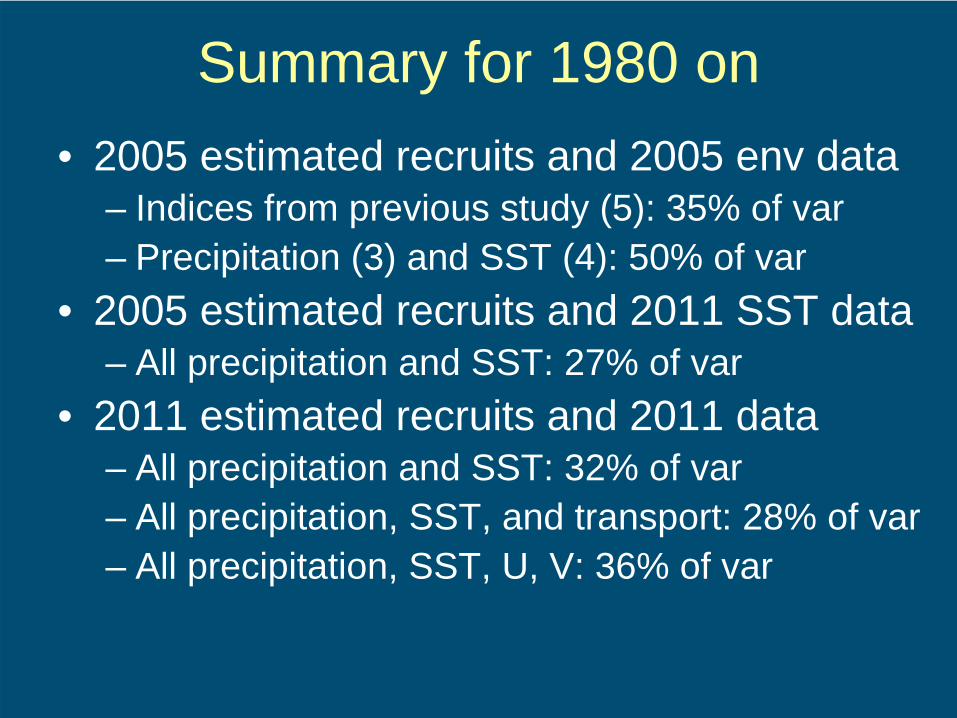
Summary for 1980 on• 2005 estimated recruits and 2005 env data
– Indices from previous study (5): 35% of var– Precipitation (3) and SST (4): 50% of var
• 2005 estimated recruits and 2011 SST data– All precipitation and SST: 27% of var
• 2011 estimated recruits and 2011 data– All precipitation and SST: 32% of var– All precipitation, SST, and transport: 28% of var– All precipitation, SST, U, V: 36% of var
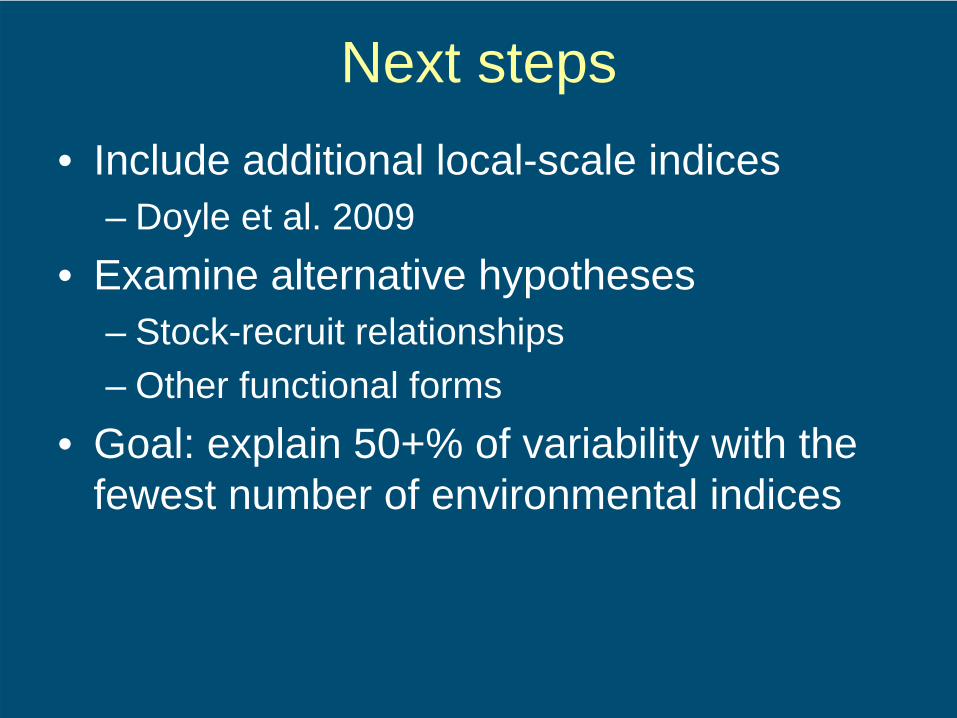
Next steps• Include additional local-scale indices
– Doyle et al. 2009• Examine alternative hypotheses
– Stock-recruit relationships– Other functional forms
• Goal: explain 50+% of variability with the fewest number of environmental indices

Thank you!