Managerial Economics & Business Strategy

Chapter 4The Theory of Individual

Behavior

McGraw-Hill/IrwinMichael R. Baye, Managerial Economics and Business Strategy Copyright © 2008 by the McGraw-Hill Companies, Inc. All rights reserved.

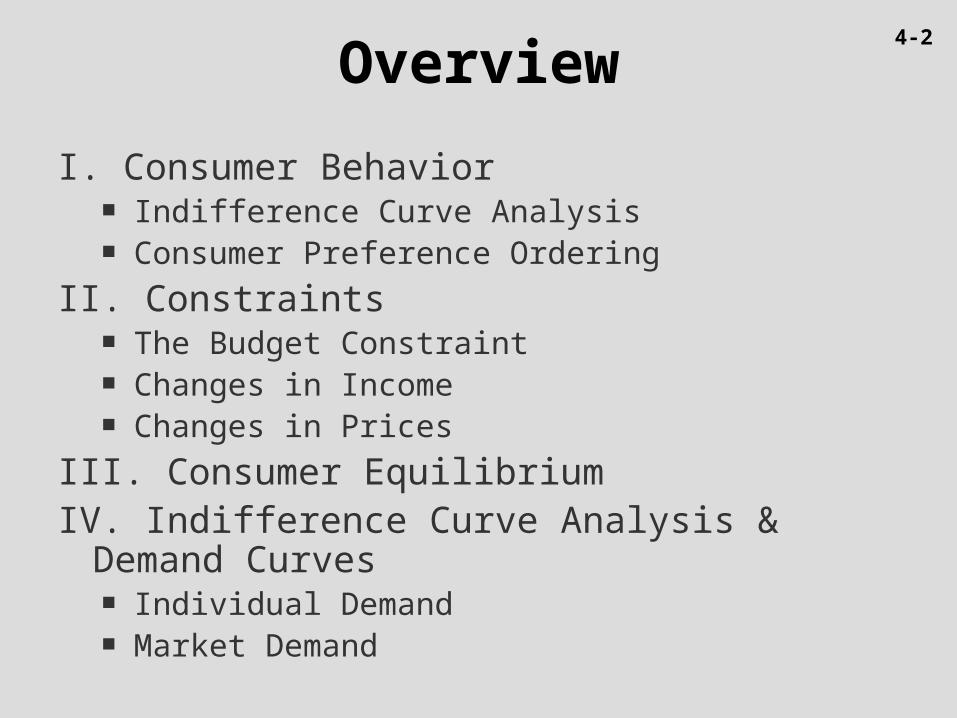
Overview

I. Consumer Behavior Indifference Curve Analysis Consumer Preference Ordering

II. Constraints The Budget Constraint Changes in Income Changes in Prices

III. Consumer EquilibriumIV. Indifference Curve Analysis & Demand Curves

Individual Demand Market Demand

4-2

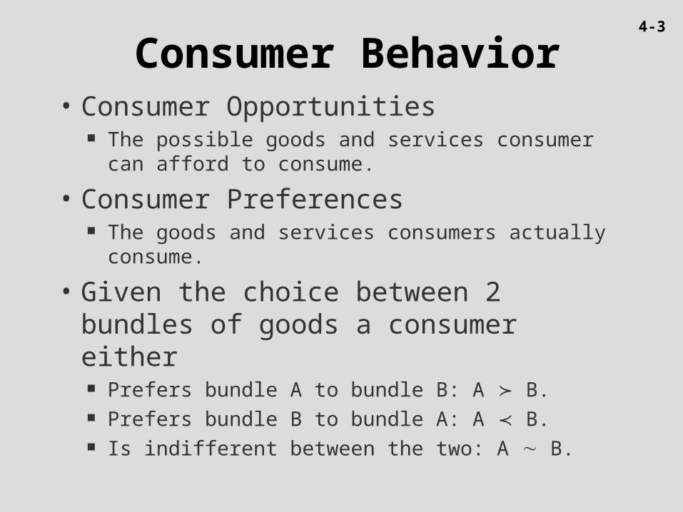
Consumer Behavior• Consumer Opportunities

The possible goods and services consumer can afford to consume.

• Consumer Preferences The goods and services consumers actually consume.

• Given the choice between 2 bundles of goods a consumer either

Prefers bundle A to bundle B: A B. Prefers bundle B to bundle A: A B. Is indifferent between the two: A B.

4-3

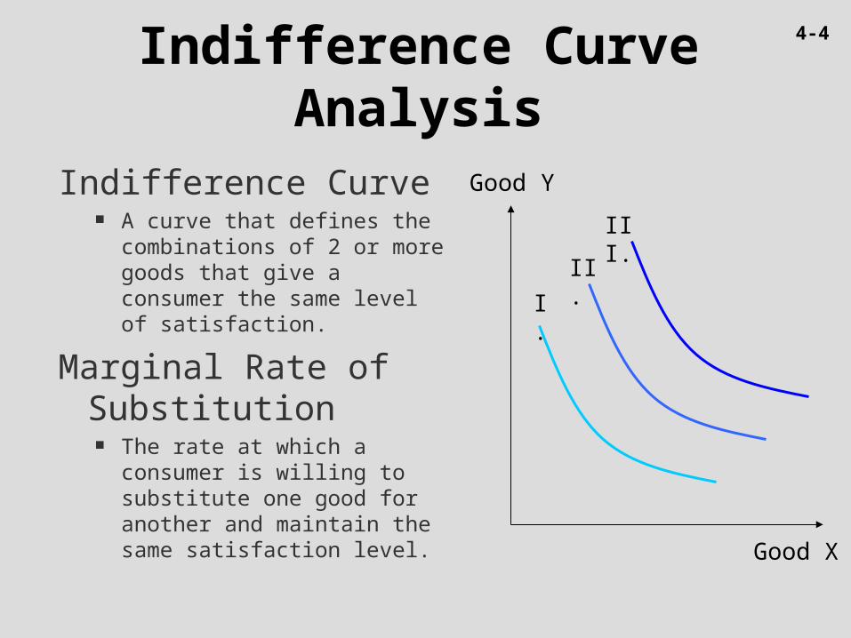
Indifference Curve Analysis

Indifference Curve A curve that defines the

combinations of 2 or more goods that give a consumer the same level of satisfaction.

Marginal Rate of Substitution

The rate at which a consumer is willing to substitute one good for another and maintain the same satisfaction level.

I.

II.

III.

Good Y

Good X

4-4

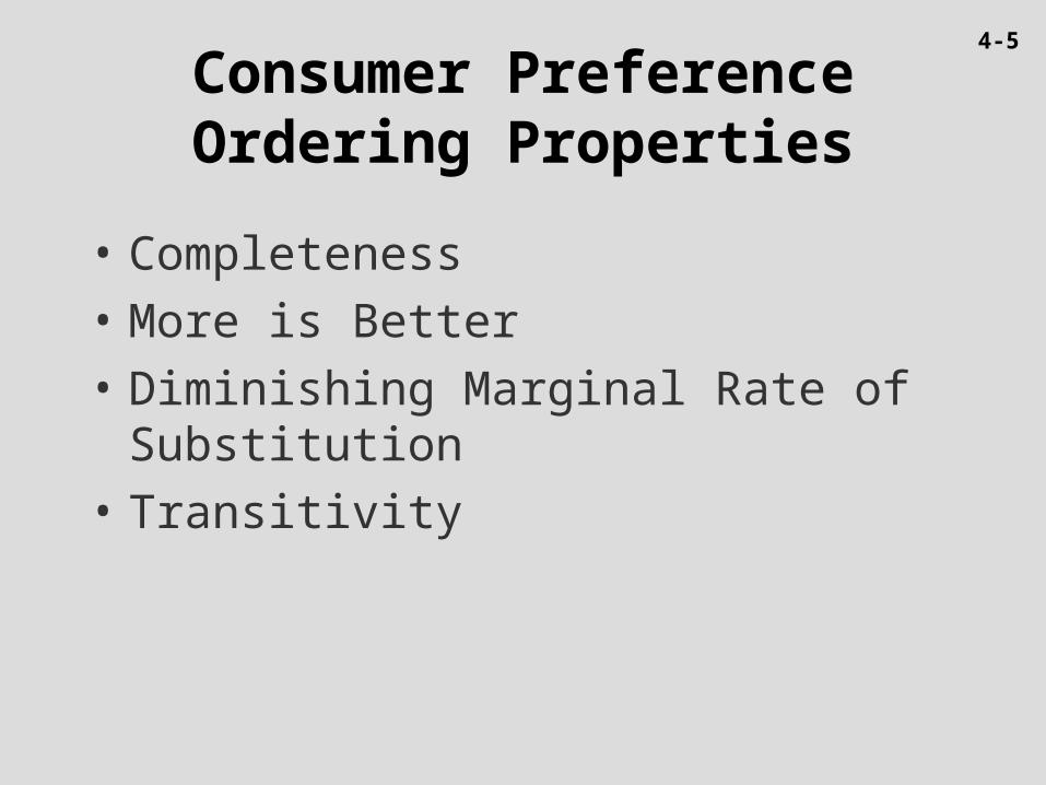
Consumer Preference Ordering Properties

• Completeness

• More is Better

• Diminishing Marginal Rate of Substitution

• Transitivity

4-5

Complete Preferences

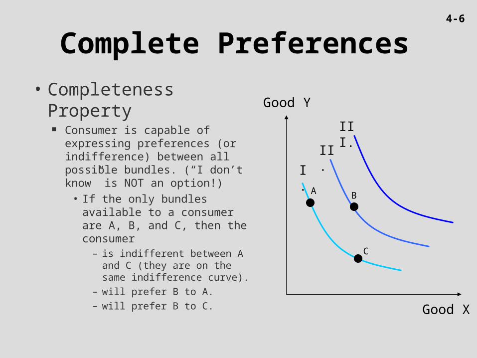
• Completeness Property Consumer is capable of

expressing preferences (or indifference) between all possible bundles. (“I don’t know” is NOT an option!)

• If the only bundles available to a consumer are A, B, and C, then the consumer

– is indifferent between A and C (they are on the same indifference curve).

– will prefer B to A.

– will prefer B to C.

I.

II.

III.

Good Y

Good X

A

C

B

4-6

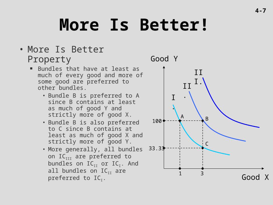
More Is Better!• More Is Better Property

Bundles that have at least as much of every good and more of some good are preferred to other bundles.

• Bundle B is preferred to A since B contains at least as much of good Y and strictly more of good X.

• Bundle B is also preferred to C since B contains at least as much of good X and strictly more of good Y.

• More generally, all bundles on ICIII are preferred to bundles on ICII or ICI. And all bundles on ICII are preferred to ICI.

I.

II.

III.

Good Y

Good X

A

C

B

1

33.33

100

3

4-7

Diminishing Marginal Rate of Substitution

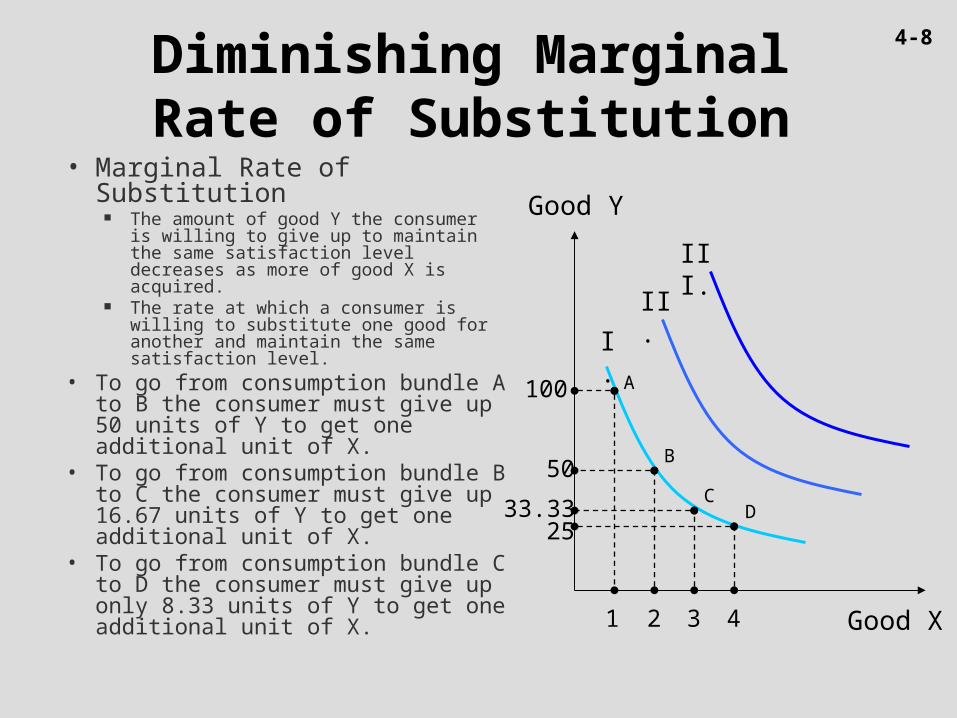
• Marginal Rate of Substitution The amount of good Y the consumer is

willing to give up to maintain the same satisfaction level decreases as more of good X is acquired.

The rate at which a consumer is willing to substitute one good for another and maintain the same satisfaction level.

• To go from consumption bundle A to B the consumer must give up 50 units of Y to get one additional unit of X.

• To go from consumption bundle B to C the consumer must give up 16.67 units of Y to get one additional unit of X.

• To go from consumption bundle C to D the consumer must give up only 8.33 units of Y to get one additional unit of X.

I.

II.

III.

Good Y

Good X1 3 42

100

50

33.33 25

A

B

CD

4-8

Consistent Bundle Orderings

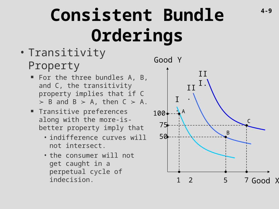
• Transitivity Property For the three bundles A, B, and

C, the transitivity property implies that if C B and B A, then C A.

Transitive preferences along with the more-is-better property imply that

• indifference curves will not intersect.

• the consumer will not get caught in a perpetual cycle of indecision.

I.

II.

III.

Good Y

Good X21

100

5

50

7

75

A

B

C

4-9

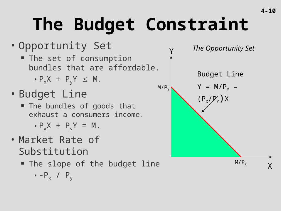
The Budget Constraint• Opportunity Set

The set of consumption bundles that are affordable.

• PxX + PyY M.

• Budget Line The bundles of goods that exhaust a

consumers income.

• PxX + PyY = M.

• Market Rate of Substitution The slope of the budget line

• -Px / Py

Y

X

The Opportunity Set

Budget Line

Y = M/PY – (PX/PY)XM/PY

M/PX

4-10

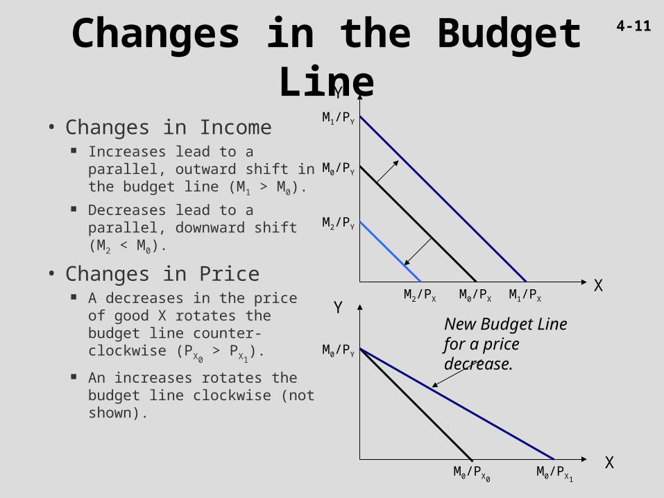
Changes in the Budget Line

• Changes in Income Increases lead to a parallel,

outward shift in the budget line (M1 > M0).

Decreases lead to a parallel, downward shift (M2 < M0).

• Changes in Price A decreases in the price of

good X rotates the budget line counter-clockwise (PX0

> PX1).

An increases rotates the budget line clockwise (not shown).

X

Y

X

YNew Budget Line for a price decrease.

M0/PY

M0/PX

M2/PY

M2/PX

M1/PY

M1/PX

M0/PY

M0/PX0M0/PX1

4-11

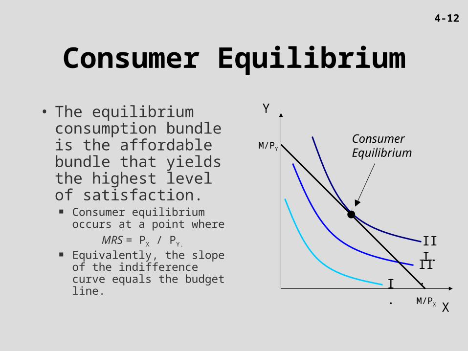
Consumer Equilibrium

• The equilibrium consumption bundle is the affordable bundle that yields the highest level of satisfaction.

Consumer equilibrium occurs at a point where

MRS = PX / PY.

Equivalently, the slope of the indifference curve equals the budget line. I.

II.

III.

X

Y

Consumer Equilibrium

M/PY

M/PX

4-12

Price Changes and Consumer Equilibrium

• Substitute Goods An increase (decrease) in the price of good X leads to

an increase (decrease) in the consumption of good Y.• Examples:

– Coke and Pepsi.– Verizon Wireless or AT&T.

• Complementary Goods An increase (decrease) in the price of good X leads to a

decrease (increase) in the consumption of good Y.• Examples:

– DVD and DVD players.– Computer CPUs and monitors.

4-13

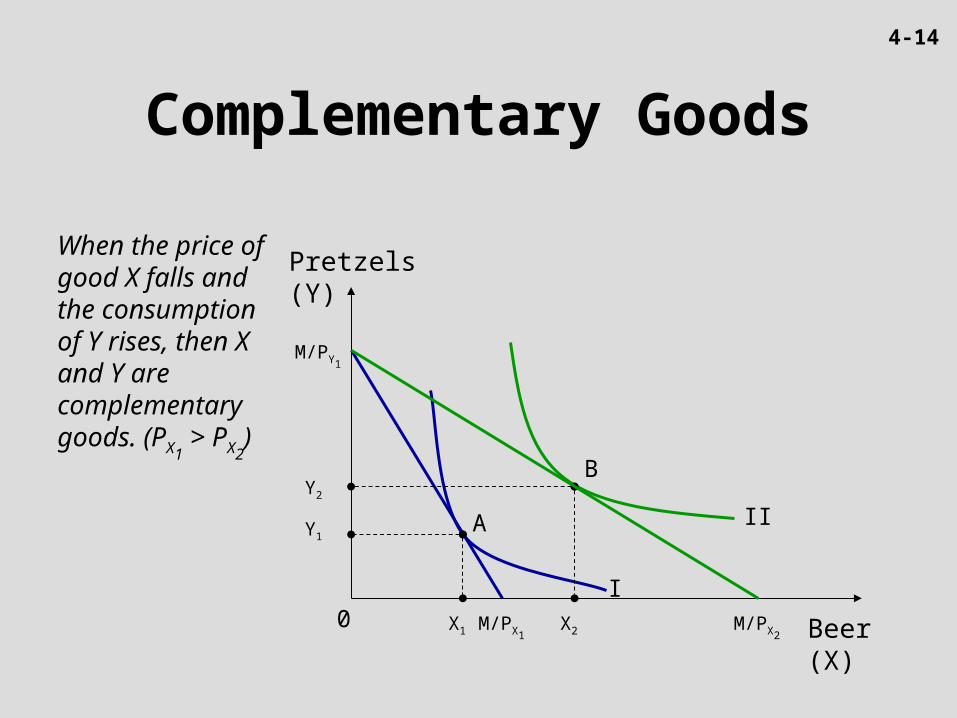
Complementary Goods

When the price of good X falls and the consumption of Y rises, then X and Y are complementary goods. (PX1

> PX2)

Pretzels (Y)

Beer (X)

II

I0

Y2

Y1

X1 X2

A

B

M/PX1M/PX2

M/PY1

4-14

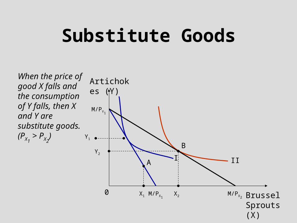
Substitute Goods

When the price of good X falls and the consumption of Y falls, then X and Y are substitute goods. (PX1

> PX2)

Artichokes (Y)

Brussel Sprouts (X)

III

0

Y2

Y1

X1 X2

A

B

M/PX1M/PX2

M/PY1

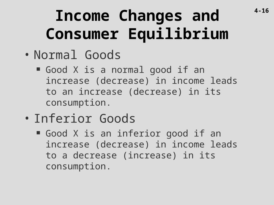
Income Changes and Consumer Equilibrium

• Normal Goods Good X is a normal good if an increase (decrease) in

income leads to an increase (decrease) in its consumption.

• Inferior Goods Good X is an inferior good if an increase (decrease) in

income leads to a decrease (increase) in its consumption.

4-16

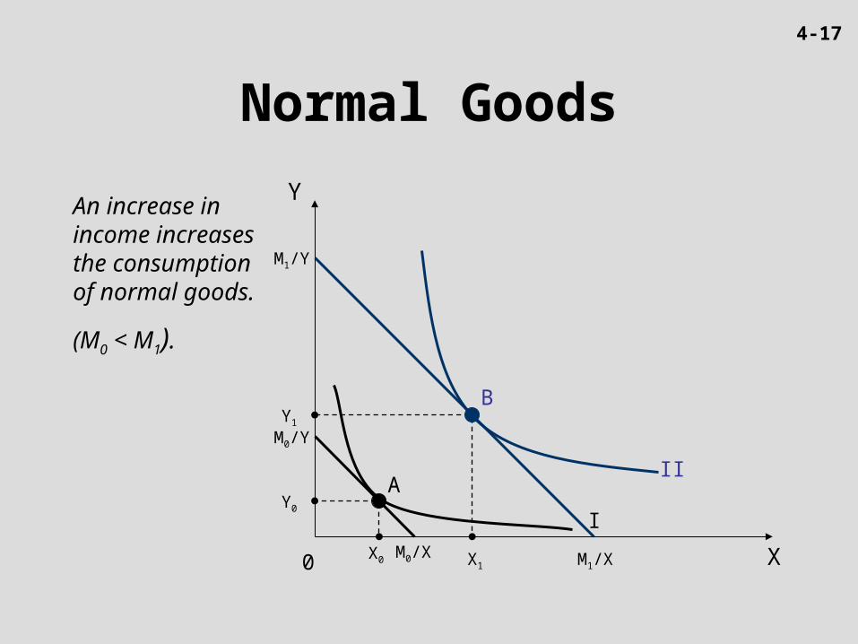
Normal Goods

An increase in income increases the consumption of normal goods.

(M0 < M1).

Y

II

I

0

A

B

X

M0/Y

M0/X

M1/Y

M1/XX0

Y0

X1

Y1

4-17

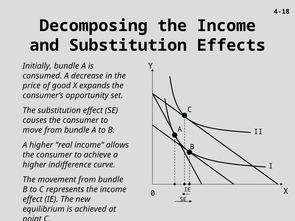
Decomposing the Income and Substitution Effects

Initially, bundle A is consumed. A decrease in the price of good X expands the consumer’s opportunity set.

The substitution effect (SE) causes the consumer to move from bundle A to B.

A higher “real income” allows the consumer to achieve a higher indifference curve.

The movement from bundle B to C represents the income effect (IE). The new equilibrium is achieved at point C.

Y

II

I

0

A

X

C

B

SE

IE

4-18

Other goods (Y)

II

I

0

A

C

B F

D

E

Pizza (X)

0.5 1 2

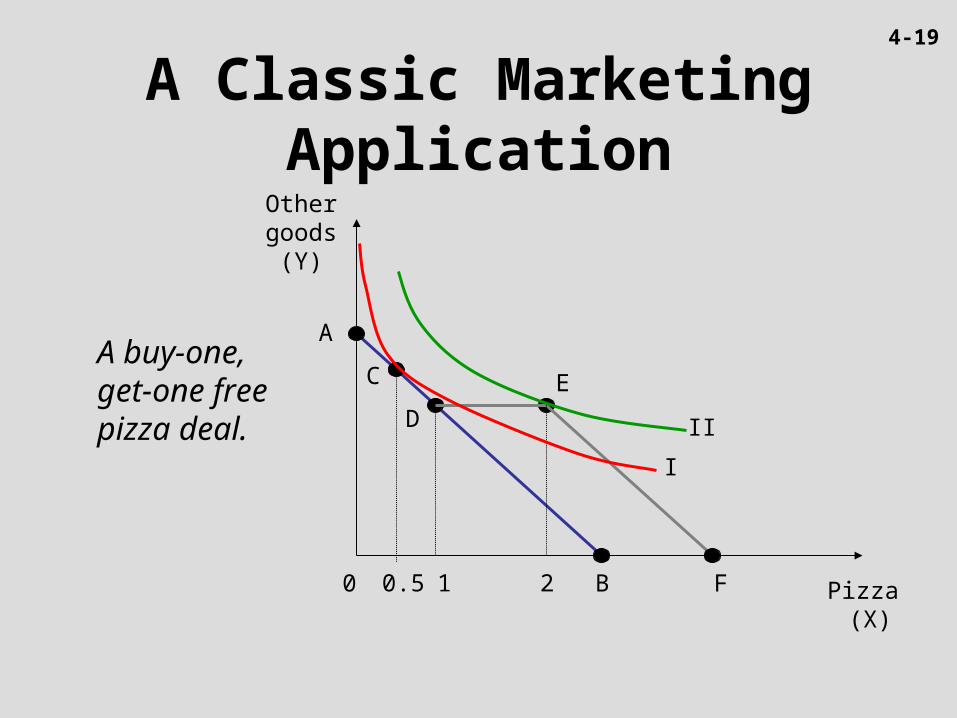
A buy-one, get-one free pizza deal.

A Classic Marketing Application

4-19

Individual Demand Curve

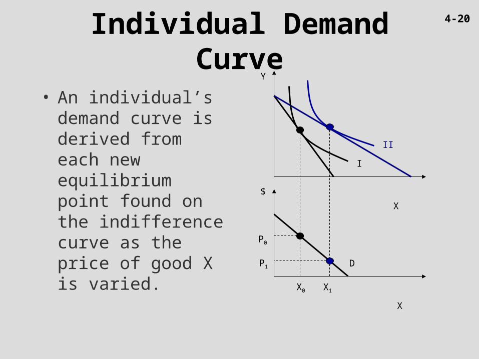
• An individual’s demand curve is derived from each new equilibrium point found on the indifference curve as the price of good X is varied.

X

Y

$

X

D

II

I

P0

P1

X0 X1

4-20

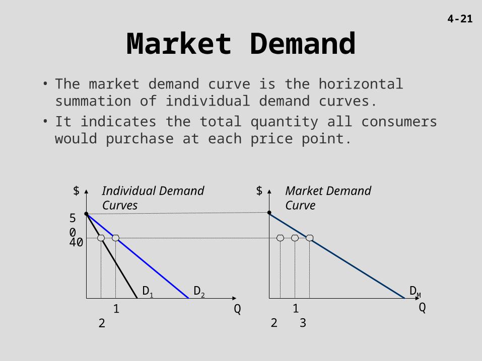
Market Demand• The market demand curve is the horizontal summation

of individual demand curves.

• It indicates the total quantity all consumers would purchase at each price point.

Q

$ $

Q

50

40

D2D1

Individual Demand Curves

Market Demand Curve

1 2 1 2 3

DM

4-21

Conclusion

• Indifference curve properties reveal information about consumers’ preferences between bundles of goods.

Completeness. More is better. Diminishing marginal rate of substitution. Transitivity.

• Indifference curves along with price changes determine individuals’ demand curves.

• Market demand is the horizontal summation of individuals’ demands.

4-22