Managerial Incentives and the Role of

Advisors in the Continuous-Time Agency

Model∗

Keiichi Hori† and Hiroshi Osano‡

March 8, 2012

Revised: September 25, 2012

Second Revised: February 17, 2013

∗The authors would like to thank Eric Chou, Yuichi Fukuta, Nobuhiko Hibara, Shinsuke Ikeda, ShingoIshiguro, Takayuki Ogawa, Yoshiaki Ogura, Jie Qin, Reijiro Samura, Luca Taschini, the editor, an anonymous

referee, and participants at the University of Tokyo, Osaka University, Ritsumeikan University, the 3rd

Florence—RitsumeikanWorkshop on "Modeling and pricing finance and insurance assets in a risk management

perspective", the 2011 Asian Meeting of the Econometric Society, and the 5th Japan—Taiwan Contract Theory

Conference for helpful comments and suggestions on an earlier version of this paper.

Correspondence to: Hiroshi Osano, Institute of Economic Research, Kyoto University, Sakyo-ku, Kyoto

606-8501, Japan.

E-mail: osano@kier.kyoto-u.ac.jp; Tel: +81-75-753-7131; Fax: +81-75-753-7138.†Faculty of Economics, Ritsumeikan University (khori@ec.ritsumei.ac.jp).‡Institute of Economic Research, Kyoto University (osano@kier.kyoto-u.ac.jp).

1

Managerial Incentives and the Role of Advisors

in the Continuous-Time Agency Model

Abstract

This paper explores a continuous-time agency model with double moral hazard. Using a

venture capitalist—entrepreneur relationship where a manager provides unobservable effort

while a venture capitalist (VC) both supplies unobservable effort and chooses the optimal

timing of the initial public offering (IPO) with an irreversible investment, we show that op-

timal IPO timing is earlier under double moral hazard than under single moral hazard. Our

results also indicate that the manager’s compensation tends to be paid earlier under double

moral hazard. We also derive several comparative static results for the IPO timing and

managerial compensation profile, all of which provide new empirically testable implications.

Usefully, even where the VC does not completely exit with the IPO, such that there is a

requirement for a multiagent analysis after the IPO, most of our results remain unchanged.

In addition, our model applies to not only the VC exit through the M&A (Mergers and

Acquisitions) process but also the dissolution of joint ventures and corporate spin-offs.

JEL Classification: D82, D86, G24, G34, M12, M51.

Keywords: two-sided moral hazard, IPO timing, managerial compensation, dynamic in-

centives, spin-offs.

2

1. Introduction

This paper examines the situation in which the joint provision of costly effort by a manager

and an advisor initially improves the productivity of a project in a firm. However, after a

substantial upward shift in productivity is achieved through irreversible investment, the

role of the advisor ends, and only the manager remains to provide ongoing costly efforts

to improve the productivity of the project. Because the timing of investment corresponds

with the timing of the change in the role of the advisor, optimal timing of investment

needs to consider the effect of this change. A difficulty may therefore arise if the manager’s

costly efforts are unobservable in that he cannot be provided with appropriate incentives.

In this case, not only the advisor’s costly efforts but also the manager’s compensation may

be controlled so as to provide the manager with appropriate incentives. In addition, the

advisor’s costly effort may be unobservable. Consequently, we must consider the provision of

incentives for effort for both the manager and the advisor when solving the optimal timing

problem of investment.

This particular situation typically arises when a venture capitalist (VC) exerts substantial

effort in monitoring managerial activity, providing managerial advice to entrepreneurs, and

choosing the optimal timing of both the initial public offering (IPO) and any investment

financed by the IPO. Indeed, the monitoring and advisory role of the VC through ongoing

long-term involvement can increase the value of its portfolio companies.1 The VC often par-

ticipates directly in management by holding one or more positions on the board of directors.

The VC also specializes in a particular industry and uses those industry contacts to help

entrepreneurs to perform various business activities.2 Furthermore, some VCs employ con-

sulting staff that are involved in the management of companies in their portfolios. However,

1The monitoring and advising role of the VC is empirically documented by Barry et al. (1990), Gompers

and Lerner (1999), Hellmann and Puri (2002), and Kaplan and Strömberg (2004).2For example, the VC helps to shape and to recruit the management team, to shape the strategy and

the business model before and after investing, to assist in production, to line up suppliers, and to develop

customer relations.

3

it is difficult to verify the intensities of such monitoring and advising efforts provided by

the VC.3 The VC can harvest investments in private companies in one of two ways; namely,

taking the firm public via an IPO or selling the firm to another company (mergers and acqui-

sitions (M&A)). In fact, we can interpret the IPO process in this paper as the M&A process

if the acquiring company’s activity or investment has a synergetic effect on the acquired

firm’s productivity. Hence, we use the terms of the “IPO” and “M&A” processes for the VC

exit route interchangeably.4

Another example is where a large established firm sells all of its claims in a joint venture

with a small innovative firm or where a parent firm spins off one of its subsidiaries to its

own shareholders and makes the subsidiary a new entity that is managed independently

of the parent firm. With joint venture dissolution, as the large established firm provides

resources in areas such as manufacturing, distribution and marketing, the large-established-

firm—small-innovative-firm relationship acts like a VC—entrepreneur relationship. With cor-

porate spin-offs, the parent firm’s CEO—subsidiary manager relationship corresponds to a

VC—entrepreneur relationship if the CEO’s objective is to maximize the initial sharehold-

ers’ payoff where the CEO is not involved in the management of the subsidiary following a

spin-off.5

To capture this dynamic problem, we develop a continuous-time agency model with double

moral hazard, in which an agent (manager) provides unobservable value-adding effort and a

principal (advisor) also contributes unobservable value-adding effort as well as choosing the

optimal timing of changing her role with irreversible investment. The basic question that we

address is how the optimal timing of changing the advisor’s role and the dynamic properties

of optimal incentive provision are characterized under double moral hazard, compared with

3The literature of optimal venture capital contracts makes a similar assumption. See Casamatta (2003),

Schmidt (2003), Repullo and Suarez (2004), Inderst and Müller (2004), and Hellmann (2006).4A similar situation occurs when buyout funds attempt to make private firms in their portfolio go public

or when banks attempt to return bankrupt firms under their administration to public ownership.5In both cases, restructuring costs need to be expended at the time of the dissolution or spin-off. Evidence

of operating performance improvements following spin-offs is in Daley, Mehrotra, and Sivakumar (1997) and

Desai and Jain (1999).

4

those under single moral hazard. We also discuss how the changes in the advisor’s role and

the manager’s compensation are interrelated. We further explore the comparative statics

regarding the timing of changing the advisor’s role and the manager’s compensation.

In our basic continuous-time agency model, the project generates cumulative cash flows

that are affected by both the principal’s and the manager’s efforts. There are complementar-

ities between the value-adding efforts of the principal and the manager. The principal also

chooses the timing of exiting; that is, the timing of the IPO and investment for achieving

an upward shift in the productivity of the project. Following the IPO, new outside investors

own the firm and induce the manager to exert an unobservable effort to operate the project,

although they cannot themselves expend any effort to operate the project.

Now, suppose as a benchmark the single moral hazard situation in which the principal’s

effort is observable and verifiable. Although the manager’s effort is unobservable, he has an

incentive to increase effort if his value depends more strongly on output. Hence, increasing

volatility of the manager’s value is required to attain a higher level of effort from the manager.

However, this implies that poor results are met with penalties. As the manager’s limited

liability precludes negative wages, the project has to be terminated inefficiently once his

future discounted payoff–that is, his continuation value–hits his outside option. Thus,

there exists a trade-off between more incentive provision and inefficient termination. This

also means that paying cash to the manager earlier makes future inefficient liquidation more

likely, as it reduces the manager’s continuation payoff. Hence, the possibility of inefficient

liquidation causes deferred compensation. Furthermore, if costly investment is irreversible,

the possibility of inefficient termination causes IPO execution to be more costly because the

investment cost is less likely to be recovered. Hence, there exists another trade-off between

earlier IPO timing and inefficient termination. This trade-off creates an option value of

waiting for an IPO. In addition, the change in the governance mechanism with the IPO also

needs to be considered in choosing the timing of the IPO, because this has a significant effect

5

on the manager’s incentives and thereby substantially affects the merit of the IPO.

We next suppose the double moral hazard situation in which the principal’s effort is

unobservable. Then, the principal may reduce her effort ex post because she may not be

able to commit to secure an appropriate ex post incentive for herself. The possibility of

a decrease in the principal’s effort may reduce the option value of waiting for the IPO (or

the principal’s expected profit obtained by waiting for the IPO), thereby advancing the IPO

timing. This possibility may also have an adverse effect on the cost of compensating the

manager for his effort and may make earlier compensation more costly under double moral

hazard. However, we will show that this final intuition is incorrect.

The main results of the model are as follows. Our first main result is that optimal IPO

timing is earlier under double moral hazard than under single moral hazard. Intuitively,

the principal’s effort supplied prior to the IPO is smaller under double moral hazard than

under single moral hazard. The reason is that under double moral hazard, the principal

has an ex post incentive to reduce her effort level, relative to that optimally obtained under

single moral hazard, because she cannot internalize the externality effect of her effort on the

manager’s incentives when choosing the level of effort after the contract has been offered.

This reduces the option value of waiting for the IPO, thus advancing the IPO timing.

The second main result is that the manager’s compensation tends to be paid earlier under

double moral hazard than under single moral hazard. Intuitively, the manager’ compensation

has never been paid before the IPO under either double or single moral hazard. Given that

the cash payment threshold is located after the IPO and that only the single moral hazard

situation arises after the IPO, the compensation payment timing is earlier under double

moral hazard because the IPO timing is earlier under double moral hazard.

We carry out the comparative static results for IPO timing and the manager’s compensa-

tion profile under double moral hazard. Then, the IPO is more likely to be brought forward

when a need for monitoring by the VC is smaller, the increment in future expected cash flows

6

is greater, and the volatility of cash flows is larger. Furthermore, the manager’s compensa-

tion tends to be paid later the smaller the increment in future expected cash flows and the

larger the volatility of cash flows. These comparative static results provide testable predic-

tions about IPO timing and vesting provisions for the manager in early-stage start-up firms,

management buyout firms, or firms reorganized following bankruptcy. These predictions can

also be tested for the dissolution of joint ventures and for corporate spin-offs.

Practically, some VCs retain a fraction of the firm’s shares and continue to hold their

board positions even after the IPO. If the principal retains a portion of the equity claims

in the firm and continues to provide effort after the IPO, a multiagent problem may arise.

Then, the analysis needs to be carried out in a multiagent setting after the IPO. We extend

our model into this case and show that most of our main results still hold. Hence, the

multiagent problem existing after an IPO does not affect our main results.

The work in this paper is related to the growing literature on continuous-time agency mod-

els using the martingale techniques developed by Sannikov (2008).6 Philippon and Sannikov

(2007) extend the cash diversion model in DeMarzo and Sannikov (2006) by considering

an endogenous shift in the timing in the mean of cash flows by irreversible investment or

IPO. However, in Philippon and Sannikov (2007), the principal supplies no effort, and a

standard Brownian motion represents a signal regarding the action of the manager, rather

than the cumulative cash flow. The main difference between our model and the aforemen-

tioned continuous-time agency models is that our model deals with a double moral hazard

situation in which the principal exerts unobservable effort to develop a project before mak-

ing an irreversible investment and exiting the firm. This enables us to investigate how the

possibility of the principal’s moral hazard affects the timing of organizational change and the

optimal properties of dynamic contract, and to explore the interplay between organizational

6See DeMarzo and Sannikov (2006), Biais, Mariotti, Plantin, and Rochet (2007), He (2009), Biais, Mar-

iotti, Rochet, and Villeneuve (2010), Hoffmann and Pfeil (2010), Jovanovic and Prat (2010), Piskorski and

Tchistyi (2010), and He (2011). The continuous-time agency model began with Holmstrom and Milgrom

(1987). However, unlike the recent model, they assume that the agent can receive a lump-sum payment only

at the end of an exogenous finite time interval (also see Sung (1997) and Ou-Yang (2003)).

7

change and the optimal properties of dynamic contract. In particular, unlike Philippon and

Sannikov (2007), under double moral hazard, we can capture the effect of a change in the

ownership structure or governance on the optimal IPO timing and compensation profile for

the manager.7 Furthermore, if the principal does not completely exit with the IPO, we are

able to explore a continuous-time multiagent model following the IPO.

Several recent studies explore optimal venture capital contracts under double moral haz-

ard.8 However, they use a discrete-time agency model with two or three periods, which is

not suitable for the analysis of the IPO timing or the dynamic optimal incentive provision.

Several existing studies have implications for firm characteristics during IPOs. Pagano

and Röell (1998) examine the effect of ownership structure on the decision to go public.

However, their model is static. Benninga, Helmantel, and Sarig (2005) and Pástor, Taylor,

and Veronesi (2009) employ a dynamic IPOmodel by trading off the diversification benefits of

going public against the benefits of private control. Both of these models suggest that going

public is optimal when cash flows or the firm’s expected future profitability is sufficiently

high. However, they do not use the continuous-time agency model, nor do they explore

the effect of the change in managerial control with the IPO (VC advice and monitoring vs.

market discipline) on the IPO timing or the manager’s compensation profile.

The paper is organized as follows. Section 2 presents a simple two-period model. Section

3 presents a continuous-time agency model. Sections 4 and 5 derive an optimal contract

under single and double moral hazard. Section 6 considers the comparative statics. Section

7 allows the principal not to exit completely with the IPO. Section 8 provides empirical

implications for our results, and Section 9 concludes.

7Our result–that the more the need for the VC’s monitoring role, the higher the IPO timing threshold–is

novel. Furthermore, Philippon and Sannikov (2007) suggest that the IPO threshold is increasing in volatility.

By contrast, our result shows that the IPO threshold may be decreasing in the risk of the project.8See the literature mentioned in footnote 3.

8

2. A Simple Two-Period Model

We begin with a simple two-period model, which will form the basis for our continuous-

time model and illustrate how our results depend on the continuous-time agency setting.

Consider a two-period model, in which a principal hires an agent to operate a firm and has

an opportunity to improve the firm’s output process substantially by undertaking irreversible

investment K when the principal exits. In the subsequent analysis, we take as an example

an IPO for a private company presently under the control of a VC or buyout fund. The

principal (the VC or buyout fund) hires a manager and then has an opportunity to exit with

an IPO. The investment cost K is paid by the funds financed from new outside investors.

The cash flows produced by the firm at time t (t = 1, 2) are given by a random variable

xt, which is jointly independent in each period. More specifically, with probability ξ ∈ (0,1), the firm cannot generate any cash flows. However, with probability 1− ξ, the firm can

generate positive cash flows.

When the positive cash flows can be generated, they depend not only on the manager’s

or principal’s effort but also on the investment involved in the IPO. More specifically, before

the IPO is undertaken, xt = αaAtaPt for α > 0, where aAt is the manager’s effort, aPt is the

principal’s effort, and α is a constant positive complementarity parameter. As the principal

makes an effort for monitoring and advising the manager to improve the firm’s business, the

efforts of the principal and the manager are interrelated before the IPO. On the other hand,

after the IPO is undertaken, xt = μaAt for μ > 1. If the IPO is undertaken, the principal

exits and provides no effort, whereas the firm is owned by new outside investors. However,

the scale of the firm expands because of the investment; thus, μ > 1.

The principal and new outside investors are risk neutral, and they discount a cash flow

stream at a riskless interest rate r. Before the IPO is undertaken, the principal chooses effort,

aPt, from the set of feasible effort levels AP , which is compact with the smallest element 0.

The principal’s effort cost function is given by η · (aPt)2, where η > 0.

9

The manager is also risk neutral but faces limited liability and discounts a cash flow stream

at a subjective discount rate γ. For simplicity, we assume that at each point in time, the

manager can choose either to shirk (aAt = 0) or to work (aAt = 1). If the manager shirks,

he receives a private benefit of shirking, h, because working is costly for the manager. The

manager’s best outside option is equal to zero in each period.

The manager can maintain a private savings account and choose how much to consume.

Neither the principal nor new outside investors can observe the balance of the manager’s

saving account. However, if the manager’s saving interest rate is lower than his discount

rate, the standard argument can show that the optimal contract does not require private

saving by the agent (see DeMarzo and Fishman (2007)). Hence, to simplify the analysis, we

assume that private saving is impossible.

The cash flows xt are publicly observable by all the agents. However, neither the principal

nor new outside investors can observe aAt. On the other hand, the manager may observe

and verify aPt or may not observe aPt.

The timing and the contract schedule are as follows.

(i) Suppose that the IPO has not been undertaken until the beginning of period t. At the

beginning of period t, the principal determines whether to undertake the IPO.

(a) If the IPO is undertaken, the principal exits the firm via the IPO, and new outside

investors can sign a contract with the manager that specifies payments wt to the manager.

After the contract is signed but before the cash flows xt are realized, the manager exerts an

effort.

(b) If the IPO is not undertaken, the principal can sign a contract with the manager that

specifies payments wt to the manager. If the manager can observe and verify aPt, the

contract can also stipulate how aPt is provided. However, if the manager cannot observe aPt,

the contract does not specify aPt. After the contract is signed but before the cash flows xt

are realized, the principal and the manager exert an effort.

10

(ii) Suppose that the IPO has been undertaken until the beginning of period t. Then, new

outside investors can sign a contract with the manager that specifies payments wt to the

manager. After the contract is signed but before the cash flows xt are realized, the manager

exerts an effort.

We start our discussion with the single moral hazard situation in which the manager can

observe and verify aPt. To simplify the analysis, we assume that h < min((1 − ξ)μ −K,

[(1−ξ)α]24η

) and that the liquidation values of the firm at t = 1 and t = 2 are equal to zero.

The game is solved through backward induction. At t = 2, the optimal contract depends

on the decision as to whether the IPO has been undertaken. Suppose that the IPO has been

undertaken. Because the realized cash flows are publicly observable, the payments w2 may

depend on x2. In the present model, x2 is always equal to zero if the manager shirks (aA2 =

0), whereas x2 is equal to μ (or 0) with probability 1 − ξ (or ξ) if the manager works (aA2 =

1). Hence, we set w2 = w20 ≥ 0 if x2 = 0, and w2 = w2+ ≥ 0 if x2 > 0. The optimal contractnow chooses (w20, w2+) so as to maximize the expected payoff of new outside investors at

t = 2 by providing incentives for the manager to work.9 This can be written as the following

optimization problem:

V I2 ≡ maxw20,w2+

− ξw20 + (1− ξ)(μ− w2+), (1)

s.t. ξw20 + (1− ξ)w2+ ≥ h.

The objective function is the expected payoff of new outside investors at t = 2 when the

manager works at t = 2. The constraint is the manager’s incentive-compatibility constraint

that induces the manager to work at t = 2. Note that the manager receives w20 (or w2+)

with probability ξ (or (1− ξ)) if he works, but always receives h if he shirks. Let (wI20, wI2+)

9If the manager shirks, the principal’s revenue is always equal to zero. Hence, under our parametric

assumption, the contract that induces the manager to shirk is not optimal. In addition, the manager’s

individual rationality constraint always holds because the manager’s best outside option is equal to zero.

This remark holds in all of the following optimization problems (1)—(4).

11

denote a solution to problem (1). Solving this problem, we obtain wI20 = 0 and wI2+ =

h1−ξ .

Substituting (wI20, wI2+) into V

I2 yields V

I2 = (1 − ξ)μ − h (> 0).

Next, suppose that the IPO has not been undertaken. The optimal contract now chooses

(w20, w2+, aP2) to maximize the expected payoff of the principal at t = 2 by providing

incentives for the manager to work. This can be written as the following optimization

problem:

V N2 ≡ maxw20,w2+,aP2

− ξw20 + (1− ξ)(αaP2 − w2+)− η · (aP2)2, (2)

s.t. ξw20 + (1− ξ)w2+ ≥ h.

The objective function is the expected payoff of the principal in this case. Note that the

principal receives αaP2 with probability 1 − ξ but must always incur the effort cost. The

constraint is the manager’s incentive-compatibility constraint which is the same as problem

(1). Let (wN20, wN2+, a

NP2) denote a solution to problem (2). Solving this problem, we obtain

wN20 = 0, wN2+ =

h1−ξ and a

NP2 =

(1−ξ)α2η

. Substituting (wN20, wN2+, a

NP2) into V

N2 leads to V N2 =

(1−ξ)2α24η

− h (> 0).We now consider whether or not the IPO is undertaken at t = 2. The principal sets the

IPO price reasonably by anticipating an incentive for the manager to choose his effort level

after the IPO. Because of arbitration, the profit of the principal from the IPO equals the

profit of new outside investors, V I2 − K. Thus, comparing V I2 − K and V N2 , we show that

the IPO is undertaken at t = 2 if μ ≥ K1−ξ +

(1−ξ)α24η

; otherwise, the IPO is not undertaken

at t = 2.

We proceed to the analysis at t = 1. In this case, we set w1 = w10 ≥ 0 if x1 = 0, and w1= w1+ ≥ 0 if x1 > 0. Note that in the present model, neither the principal nor new outsideinvestors have any incentive to vary the manager’s continuation value in order to induce the

manager to work at t = 1, because the contract termination date is exogenous under the

stationary environment.10

10Define U20 (U2+) as the manager’s expected payoff at t = 2 conditional on x1 = 0 (x1 > 0). Because the

12

Suppose that the IPO is undertaken at t = 1. Then, the principal exits at both t = 1 and

2. Thus, the optimal contract chooses (w10, w1+) so as to maximize the sum of the expected

payoffs of new outside investors at t = 1 and 2 by providing incentives for the manager to

work. Indeed, the period 2 optimal contract is given by the solution to problem (1) in this

case because the IPO was undertaken at t = 1. Hence, the optimization problem is given by

V I1 ≡ maxw10,w1+

− ξw10 + (1− ξ)(μ− w1+) + 1

1 + rV I2 , (3)

s.t. ξw10 + (1− ξ)w1+ ≥ h.

Let wI10 and wI1+ denote a solution to problem (3). As V

I2 does not depend on (w10, w1+), we

obtain wI10 = 0, wI1+ =

h1−ξ , and V

I1 = (1 − ξ)μ − h + 1

1+rV I2 .

When the IPO is not undertaken at t = 1, the optimal contract chooses (w10, w1+, aP1)

so as to maximize the sum of the expected payoffs of the principal at t = 1 and t = 2 by

providing incentives for the manager to work and considering the possibility of the IPO at

t = 2. Then, the period 2 optimal contract is given by the solution to problem (1) or (2)

according as the IPO is undertaken or not at t = 2. The optimization problem is then

V N1 ≡ maxw10,w1+,aP1

− ξw10 + (1− ξ)(αaP1 − w1+)− η · (aP1)2 + 1

1 + rmax(V I2 −K,V N2 ), (4)

s.t. ξw10 + (1− ξ)w1+ ≥ h.

Note that the principal’s profit from the IPO at t = 2 is equal to V I2 −K. Let (wN10, wN1+, aNP1)denote a solution to problem (4). As V I2 and V

N2 do not depend on (w10, w1+, aP1), solving

this problem yields wN10 = 0, wN1+ =

h1−ξ , a

NP1 =

(1−ξ)α2η

, and V N1 =(1−ξ)2α2

4η− h + 1

1+rmax(V I2 −

K,V N2 ).

Comparing V I1 − K and V N1 , we show that the IPO is undertaken at t = 1 if μ ≥ (1+r)K

(1−ξ)(2+r)

manager needs to be induced to work at t = 2, in the present model, the optimal contract at t = 2 implies

that U20 = U2+ = h, regardless of whether or not the IPO is undertaken at t = 2.

13

+(1−ξ)α24η

; otherwise, the IPO is not undertaken at t = 1. Given that the IPO is undertaken

at t = 2 only if μ ≥ K1−ξ +

(1−ξ)α24η

, this result implies that the IPO would be undertaken

immediately at t = 1, or it would never be done at any time.

Under the double moral hazard situation in which the manager cannot observe aPt, the

principal’s maximization problems of (2) and (4) do not change because neither the princi-

pal’s future expected value nor the manager’s incentive-compatibility constraint depends on

the principal’s effort. Hence, the principal has no incentive to deviate from her effort level

recommended by the optimal contract. Thus, the equilibrium contract under double moral

hazard is the same as that under single moral hazard.

To summarize, in the discrete two-period model, we obtain the following results.

Results: (i) There is no difference between the equilibria attained under the single and

double moral hazard situations.

(ii) In equilibrium, the IPO would be undertaken immediately at t = 1, or it would never

be done at any time. Neither the payments to the manager nor the principal’s effort varies

over time.

The discrete two-period framework, however, restricts our analysis in several respects.

First, even though the cash flows are independent and identically distributed, the dynamic

incentive-compatibility constraint for the manager may depend on the principal’s effort if

the endogenous threat of contract termination makes the optimal contract depend on the

manager’s continuation value because such a contract gives stronger incentive for the manager

to work hard in order to avoid the possibility of contract termination. Then, the principal

needs to consider the effect of her effort on the future expected payoffs of the principal

and the manager. This creates a difference between the equilibria under single and double

moral hazard. In addition, the principal’s effort may vary over time. Second, if the optimal

contract depends on the manager’s continuation value, the IPO would not be undertaken

until the manager’s future expected payoff is sufficiently high. This is because the possibility

14

of future contract termination should be sufficiently small to recover the IPO cost. Hence,

it is very unlikely that the IPO would be undertaken immediately at the initial time or it

would never be done at any time. Third, if the optimal contract depends on the manager’s

continuation value, an incentive for the manager can be given by varying his continuation

payoff instead of paying him cash in the current period. Then, the manager’s compensation

may not be paid in order to induce him to make more effort. As we will show in the

subsequent sections, moving in the continuous time framework with the endogenous threat

of contract termination relaxes these restrictions of the discrete two-period framework and

provides additional insights from the dynamic perspective.

3. Continuous-Time Agency Model

We now consider a continuous-time version of the principal—agent model. Again, we take

as an example the IPO described in the preceding section. A principal (a VC or buyout

fund) hires a manager and then has an opportunity to exit with an IPO. The irreversible

investment cost K at the IPO is then financed by the funds from new outside investors in

the IPO.

Let Xt denote the cumulative cash flows produced by the firm up to time t. The total

output Xt evolves according to

dXt = Atdt+ σdZt, (5)

where At is the drift of the cash flows, σ is the instantaneous volatility, and Z = Zt,Ft; 0 ≤t < ∞ is a standard Brownian motion on the complete probability space (Ω,F , Q). Morespecifically, before the investment with the IPO, At is represented by

At = aAt + ζaPt + αaAtaPt,

where aAt is the manager’s effort, aPt is the principal’s effort, ζ is a constant nonnegative

15

scale adjusted parameter, and α is a constant nonnegative complementarity parameter. As

the principal makes an effort to monitor and advise the manager in order to improve the

firm’s business,11 the efforts of the principal and the manager are interrelated before the

IPO. However, after the investment with the IPO, for μ > 1

At = μaAt.

If the IPO is undertaken, the principal exits, and the firm is now owned by new outside

investors. Thus, aPt = 0. However, the scale of the firm expands because of the investment;

thus, μ > 1.

The principal and new outside investors are risk neutral and discount the flow of profit at

rate r. The principal’s effort is a stochastic process aPt ∈ AP , 0 ≤ t ≤ τ I progressivelymeasurable with respect to Ft, where the set of her feasible effort levels AP is compact withthe smallest element 0, and τ I is the time of the IPO. The principal’s effort cost function

g(aPt)–measured in the same units as the flow of profit–is an increasing, convex, and C2

function. We normalize g(0) = 0.

The manager is risk neutral, but a negative wage is ruled out by limited liability. In

addition, the manager also discounts his consumption at γ (> r).12 If the manager’s saving

interest rate is lower than the principal’s discount rate and if the manager is risk neutral,

DeMarzo and Sannikov (2006) show that there is an optimal contract in which the manager

maintains zero savings. Hence, in this model, the manager can be restricted to consuming

11In the monitoring—auditing model of Townsend (1979), the informed agent asks for costly state verifi-

cation so that the realization of the project returns is made known to the uninformed agent. As the costly

verification in equilibrium occurs only in the low-revenue states, the monitoring and auditing of his model

naturally corresponds to bankruptcy proceedings. Hence, the monitoring and auditing cannot increase the

productivity of the firm. By contrast, in our model, the principal, who is uninformed about the manager’s

effort, monitors and advises the manager, who is informed or uninformed about the principal’s effort, as

discussed in the introductory section. As a result, the monitoring and advising of our model can increase

the productivity of the firm although it cannot make the manager’s effort known to the principal.12If the principal and the manager are equally patient when the manager is risk neutral, the principal

can postpone payments to the manager indefinitely. This possibility precludes the existence of an optimal

contract. See Biais, Mariotti, Rochet, and Villeneuve (2010).

16

what the principal pays him at any time. To simplify the analysis, we assume that at each

point of time, the manager can choose either to shirk (aAt = 0) or to work (aAt = 1), where

AA = 0, 1. Because working is costly for the manager or shirking results in a privatebenefit, we also suppose that the manager receives a flow of private benefit equal to hdt if

he shirks.

The total output process Xt, 0≤ t <∞ is publicly observable by all the agents. However,neither the principal nor new outside investors can observe aAt ∈ AA, 0 ≤ t < ∞ or theflow of the manager’s private benefit, whereas the manager may observe and verify aPt ∈AP , 0 ≤ t ≤ τ I or may not observe aPt ∈ AP , 0 ≤ t ≤ τ I.For 0 ≤ t ≤ τ I , the principal can sign a contract with the manager at time t = 0 that

specifies how the manager’s nondecreasing cumulative consumption, Ct, depends on the

observation of Xt.13 If the manager can observe and verify aPt ∈ AP , 0 ≤ t ≤ τ I, the

contract can also stipulate how aPt depends on the observation of Xt. Let Π = Ct, aPt :0 ≤ t ≤ τ I denote the contract prior to the IPO if the manager can observe and verify aPt∈ AP , 0 ≤ t ≤ τ I; and ΠD = Ct : 0 ≤ t ≤ τ I denote the contract prior to the IPO if themanager cannot observe aPt ∈ AP , 0 ≤ t ≤ τ I. On the other hand, for τ I ≤ t < ∞, newoutside investors can sign a contract with the manager at time t = τ I that specifies how Ct

depends on the observation of Xt. Let Π = Ct : τ I ≤ t <∞ denote the contract after theIPO. The principal and new outside investors are able to commit to any such contract. In

addition, the principal determines how the time of the IPO, τ I , depends on the observation

of Xt and how the time when the contract is terminated before the IPO, τT0, depends on the

observation of Xt. New outside investors also determine how the time when the contract is

terminated after the IPO, τT1, depends on the observation of Xt.

Now, for any contract Π (or ΠD) and Π and for any time (τ I , τT0 , τT1), suppose that

the manager chooses an effort-level process aAt ∈ AA, 0 ≤ t < ∞. The manager’s total13Because a negative wage is ruled out, note that Ct is nondecreasing.

17

expected payoff at t = 0 is then

E

½Z τT0I

0

e−γt [dCt + h · (1− aAt)dt] + 1τI≥τT0e−γτT0R

+ 1τI<τT0e−γτI

∙Z τT1

τI

e−γ(t−τI) [dCt + h · (1− aAt)dt]¸+ 1τI<τT0e

−γτT1R

¾, (6)

where τT0I = min(τT0 , τ I); 1τI≥τT0 = 1 or 0 (1τI<τT0 = 0 or 1) according to τ I ≥ τT0 or τ I <

τT0 ; and the manager receives expected payoff R from an outside option when the contract

is terminated, irrespective of whether or not the IPO occurs. In addition, for any contract Π

(or ΠD) and Π and for any time (τ I , τT0 , τT1), suppose that the principal and the manager

choose effort-level processes aPt ∈ AP , 0 ≤ t ≤ τ I and aAt ∈ AA, 0 ≤ t <∞. Then, theprincipal’s total expected profit at t = 0 is

E

½Z τT0I

0

e−rt [(aAt + ζaPt + αaAtaPt − g(aPt)) dt− dCt] + 1τI≥τT0e−rτT0L0

+ 1τI<τT0e−rτI

∙Z τT1

τI

e−r(t−τI)(μaAtdt− dCt)−K¸+ 1τI<τT0e

−rτT1L1

¾, (7)

where L0 (L1) is the expected liquidation payoff of the principal (new outside investors) when

the contract is terminated before (after) the IPO. Note that at t = τ I , new outside investors

buy the firm via the IPO. The principal anticipates an incentive for the manager to choose

his effort level after the IPO and sets the IPO price reasonably. Because of arbitration, the

principal’s profit from the IPO equals the total expected payoff of new outside investors at t

= τ I exclusive of the IPO cost, which is represented by the third and fourth terms in (7).14

To conclude this section, we show how the optimal contract is implemented with standard

compensation contracts and the IPO process. Up to the time of the IPO, τ I , the principal

receives the net revenue produced by the firm, dXt − dCt, at each time t. At time τ I ,

14In corporate spin-offs, the shares of the subsidiary are distributed on a pro rata basis to the parent firm’s

shareholders. If the principal is the parent firm’s CEO whose preferences therefore coincide with those of

the parent firm’s shareholders, her objective function is still given by (7) because of not being involved in

the management of the spun-off subsidiary.

18

the principal sells the firm’s shares to new outside investors via the IPO and finances the

investment cost K. After τ I , new outside investors receive the net revenue produced by

the firm, dXt − dCt, at each time t. The manager receives compensation dCt at each timet, both before and after the IPO. Although the compensation contract prior to the IPO is

separate from that after the IPO, the former can specify the manager’s compensation dCt

at each time t prior to the IPO and the manager’s continuation payoff WI at the time of

the IPO, as discussed in Philippon and Sannikov (2007). At time τ I , the manager and new

outside investors can commit to the post-IPO compensation contract dCt at each time t,

because they do not have any incentive to renegotiate at time τ I .15

4. Optimal Contract in a Single Moral Hazard Situation

In this section, we assume that the manager can observe and verify aPt ∈ AP , 0 ≤ t

≤ τ I. Thus, the principal need not design the contract to provide an appropriate ex postincentive for herself. We now derive the optimal contract in two steps. First, we obtain the

optimal contract after the IPO, assuming that the IPO was made at t = τ I . Then, given

the post-IPO value function, we characterize the optimal contract before the IPO, and the

optimal timing of the IPO.

4.1. Optimal contract after the IPO.–

Consider the case where the IPO has already taken place. The contracting problem is then

to find a combination of an incentive-compatible contract and termination timing, (Π, τT1),

and an incentive-compatible choice of the manager’s effort process, aAt ∈ AA, τ I ≤ t ≤ τT1,that maximize the expected profit of new outside investors subject to delivering the manager

a required payoff WI at the IPO, where WI is defined by the manager’s continuation value

Wt at t = τ I given below. The manager’s effort process is incentive compatible with respect

to (Π, τT1) if it maximizes his total expected payoff from τ I onward given (Π, τT1); that is,

15The proof is similar to that in Philippon and Sannikov (2007).

19

if it maximizes EτI

½Z τT1

τI

e−γ(t−τI)[dCt + h · (1− aAt)dt] + e−γ(τT1−τI)R¾.

To characterize the optimal contract, we can write the contracting problem recursively

with the manager’s continuation utility as the single state variable. For any (Π, τT1), the

manager’s continuation value Wt is his future expected discounted payoff at time t, given

that he will follow aAt ∈ AA, τ I ≤ t ≤ τT1:

Wt = Et

½Z τT1

t

e−γs [dCs + h · (1− aAs)ds] + e−γ(τT1−t)R¾. (8)

In other words,Wt represents the manager’s continuation value obtained under (Π, τT1) when

he plans to follow aAt from t onward. The manager’s consumption and effort process is then

specified by C(Wt), aA(Wt) : τ I ≤ t ≤ τT1. Denote by G(W ) the value function of newoutside investors before deducting the investment costK (the highest expected present value

of the profit to new outside investors that can be obtained from a contract that provides the

manager with the continuation value W ). To simplify our discussion, we assume that G(W )

is concave. The formal proof for the concavity of G(W ) will be provided in the Appendix.

The optimal contract is now derived using the technique in DeMarzo and Sannikov (2006)

and Sannikov (2008). For the present, we assume that implementing the manager’s high

effort at any t ∈ [τ I , τT1 ] is optimal for new outside investors. After presenting Proposition2, we give a simple sufficient condition for the manager’s high effort to remain optimal for

all W ∈ [R, W++] by following the arguments of DeMarzo and Sannikov (2006).

First, Proposition 1 expresses the evolution of Wt and provides a necessary and sufficient

condition for the manager’s effort process to be incentive compatible.

Proposition 1: For any (Π, τT1), there exists a progressively measurable process Yt,Ft :

20

τ I ≤ t ≤ τT1 in L∗ such that16

dWt = γWt − h · [1− aA(Wt)]dt− dC(Wt) + Y (Wt)[dXt − μaA(Wt)dt], (9)

for every t ∈ [τ I , τT1]. Implementing the manager’s high effort (aA(Wt) = 1) is incentive

compatible with respect to Π if and only if

Y (Wt)μ ≥ h, t ∈ [τ I , τT1]. (10)

Proof: Given that the manager is risk neutral, that aAt = 1 if he works, and that aAt =

0 and he receives hdt if he shirks, we can prove this statement by applying the proofs of

Propositions 1 and 2 in the Appendix in Sannikov (2008). ¥

The evolution of Wt in (9) depends on a drift component that corresponds to promise

keeping, and a diffusion component that links to the manager’s effort choice and provides

him with incentives. The drift component implies that Wt has to grow at the manager’s

discount rate γ, while it must decrease with dC(Wt) + h · [1− aA(Wt)] dt. The diffusion

component expressed by the final term in (9) is related to the manager’s incentives. Here,

Y (Wt) is the sensitivity of the manager’s continuation value to output. If the manager

deviates from a recommended effort level, his actual effort affects only the flow of private

benefit and the drift of Xt of (5) after the IPO, because the other parts are predetermined

by the contract. Hence, taking the contract Π as given, the manager has an incentive to

choose aA ∈ 0, 1 that maximizes the sum of the expected change of Wt and the flow of

private benefit; that is, Γ1(aA) ≡ Y (Wt)μaA + h · (1−aA). If implementing the agent’s higheffort is incentive compatible, this means that Γ1(1) ≥ Γ1(0), which is equivalent to (10).

Let

β1 ≡ min y : yμ ≥ h =h

μ. (11)

16A process Y is in L∗ if E∙Z t

0

Y 2s ds

¸<∞ for all t ∈ [0,∞).

21

It is costly to expose the manager to risk. Hence, as argued in DeMarzo and Sannikov (2006)

and Sannikov (2008), in the optimal contract, the principal must set Y (Wt) at the minimal

level that induces high effort level aA(Wt) = 1, which satisfies the manager’s incentive-

compatibility constraint (10). It follows from (11) that β1 is such a minimum level and

satisfies (10).

As proved in DeMarzo and Sannikov (2006), the optimal compensation policy depends on

G0(W ). Indeed, as new outside investors have the option to give dC units of consumption to

the manager and move to the optimal contract with W − dC, the optimality of the contractimplies G(W ) ≥ G(W − dC) − dC. Because the marginal cost of delivering the manager’scontinuation payoff can never exceed the cost of an immediate transfer in terms of the utility

of new outside investors, we must have G0(W ) ≥ −1. Define W++ as the lowest value of W

such that G0(W ) = −1. Then, it is optimal to set the manager’s compensation as

dC(W ) = max (W −W++, 0).

This compensation and the option to terminate keep the manager’s continuation payoff

between R and W++.

Now, the following proposition summarizes the optimal contract after the IPO.

Proposition 2: For the manager’s starting value WI ∈ [R, W++], the optimal contract

is characterized by the unique concave function G(W ) that satisfies the Hamilton—Jacobi—

Bellman (HJB) equation

rG(W ) = maxY≥β1

μ+G0(W )γW +G00(W )2

Y 2σ2, (12)

with β1 =hμand boundary conditions

G(R) = L1, G0(W++) = −1, and G00(W++) = 0. (13)

22

When Wt ∈ [R, W++), dC(Wt) = 0. When Wt = W++, payments dCt cause Wt to reflect

at W++. If Wt > W++, an immediate payment Wt − W++ is made. The contract is

terminated at time τT1 when Wt hits R for the first time. The optimal contract then attains

profit G(WI) for new outside investors.17

Proof: See the Appendix. ¥

As G00(W ) < 0, new outside investors dislike volatility in W and optimally choose the

sensitivity of W to output; that is, Y = β1 =hμin (12). The first boundary condition of

(13) is the value-matching condition, which implies that the principal must terminate the

contract to hold the agent’s reservation value, R. The second boundary condition is the

smooth-pasting condition that guarantees the optimal choice of W++. The third boundary

condition of (13) is the super contract condition for the optimal choice of W++, which

requires that the second derivatives match at the boundary. Using equations (12) and (13),

this condition means that rG(W++) + γW++ = μ; that is, payment to the manager is

postponed until the new outside investors’ and manager’s required expected returns exhaust

the available expected cash flows generated after the IPO. These boundary conditions fix

the solution to the HJB equation in (12).

Finally, we provide a simple sufficient condition for the manager’s high effort to be optimal

at any t ∈ [τ I , τT1 ]. Let W S ≡ hγdenote the manager’s discounted payoff if the manager

shirks forever, and let WmaxG denote the value of W that achieves the greatest value of

G(W ) in the range of W ∈ [R, W++]. Then, we obtain the following lemma.

Lemma 1: Implementing the manager’s high effort at any t ∈ [τ I , τT1 ] is optimal for newoutside investors if

γ

rG(WS) + (1− γ

r)G(WmaxG) ≥ 0. (14)

Proof: See the Appendix. ¥17For any starting value of WI > W++, G(WI) is an upper bound on the total expected profit of new

outside investors. However, this case can be excluded because F 0(WI) = G0(WI) > −1, as will be shown in

Proposition 4. If WI < R, the manager never participates in the contract.

23

Intuitively, the condition of (14) ensures that the payoff rate of new outside investors

from letting the manager shirk will be less than that under our existing contract. DeMarzo

and Sannikov (2006, Proposition 8) derive a similar condition, but their condition is more

stringent than (14) if the expected cash flow is larger than the agent’s shirking private benefit.

The condition of (14) implies a lower bound on W S, or equivalently, h.

4.2. Optimal contract before the IPO.–

In this case, the contracting problem is to find a combination of an incentive-compatible

contract and IPO and termination timing, (Π, τ I , τT0), and an incentive-compatible man-

ager’s effort process, aAt ∈ AA, 0 ≤ t < ∞, that maximize the expected profit of theprincipal subject to delivering the manager an initial required payoff W0. The manager’s ef-

fort process is incentive compatible with respect to (Π, τ I , τT0) if it maximizes the manager’s

total expected payoff defined by (6), given (Π, τ I , τT0).

Given Wt as in (8), the processes of the manager’s consumption and the manager’s and

principal’s efforts can be specified by C(Wt), aA(Wt), aP (Wt) : 0 ≤ t ≤ τT0I. Denote byF (W ) the value function of the principal. To facilitate our discussion, we assume that F (W )

is concave. The formal proof for the concavity of F (W ) will be provided in the Appendix.

For the present, we again assume that implementing the manager’s high effort (aA(Wt)

= 1) at any t ∈ [0, τT0I ] is optimal for the principal. After we present Proposition 4, weprovide a simple sufficient condition for the manager’s high effort to remain optimal at any

t ∈ [0, τT0I ].Now, as in Proposition 1, we obtain the following proposition.

Proposition 3: For any (Π, τ I , τT0), there exists a progressively measurable process Yt,Ft: 0 ≤ t ≤ τT0I in L∗ such that

dWt = γWt − h · [1− aA(Wt)] dt−dC(Wt)+Y (Wt)dXt−[aA(Wt)+ζaP (Wt)+αaA(Wt)aP (Wt)]dt,(15)

24

for every t ∈ [0, τT0I ]. Implementing the manager’s high effort (aA(Wt) = 1) is incentive

compatible with respect to Π if and only if

Y (Wt) [1 + αaP (Wt)] ≥ h, t ∈ [0, τT0I ]. (16)

Proof: Note that the manager is risk neutral, that aAt = 1 if he works, and that aAt = 0 and

the manager receives hdt if he shirks. Then, we can prove this statement using a procedure

similar to that in the proofs for Propositions 1 and 2 in the Appendix in Sannikov (2008).

¥

As in (9), the evolution of Wt in (15) depends on a predetermined drift part that cor-

responds to promise keeping and a diffusion part that links to the manager’s effort choice

and also provides him with incentives. Taking the contract Π as given, the manager has

an incentive to choose aA ∈ 0, 1 that maximizes the sum of the expected change of Wt

and the flow of private benefit; that is, Γ0(aA, aP (Wt)) ≡ Y (Wt)[aA + αaAaP (Wt)] + h · (1− aA). If implementing the manager’s high effort is incentive compatible, this means thatΓ0(1, aP (Wt)) ≥ Γ0(0, aP (Wt)), which is equivalent to (16).

Before proceeding further, we make the following assumption according to Sannikov (2008).

Assumption 1: The sensitivity is bounded from below by β (> 0) such that Y (W ) ≥ β.

Assumption 1 gives a positive lower bound of Y (W ), which ensures that the manager’s

incentives can be controlled. Note that β can be chosen as a sufficiently small positive

number so that there is no restriction on the optimal solution.

We also make the following assumption, which ensures that the IPO does not take place

at time 0 if W0 is not sufficiently large.

Assumption 2: K > max(L0, L1).

Let

β0(aP ) = min y : y · (1 + αaP ) ≥ h = h

1 + αaP. (17)

25

Because it is costly to expose the manager to risk, in the optimal contract, the principal must

set Y (Wt) at the minimal level that induces the high effort level (aA = 1), which satisfies

the manager’s incentive-compatibility constraint (16). It follows from (17) that β0(aP ) is

such a minimum level and satisfies (16). Again, the optimal compensation policy depends

on F 0(W ) because we must have F (W ) ≥ F (W − dC) − dC or F 0(W ) ≥ −1. Define W+

as the lowest value of W such that F 0(W ) = −1. Then, it is optimal to pay the manageraccording to

dC(W ) = max (W −W+, 0).

In fact, as in Proposition 4, we will show that W+ ≥ WI . Thus, we can indicate that the

manager’s compensation is zero before the IPO.

Now, the following proposition summarizes the optimal contract before the IPO.

Proposition 4: Suppose that the manager can observe and verify aPt ∈ AP , 0 ≤ t ≤τT0I. For any starting value W0 ∈ [R,WI ], the optimal contract is characterized by the

unique concave function F (W ) (≥ G(W ) − K) that satisfies the HJB equation

rF (W ) = maxaP∈AP ,Y≥β0(aP )

1 + (ζ + α)aP − g(aP ) + F 0(W )γW +F 00(W )2

Y 2σ2, (18)

with β0(aP ) =h

1+αaPand boundary conditions

F (R) = L0, F (WI) = G(WI)−K, and F 0(WI) = G0(WI). (19)

When Wt ∈ [R,WI ], dC(Wt) = 0. This means WI ≤W+. The IPO occurs when Wt reaches

WI (> R), or the contract is terminated when Wt hits R, whichever happens sooner. After

the IPO, the continuation contract is given by Proposition 2 at the starting value WI. The

optimal contract then provides profit F (W0) to the principal.18

18For the starting value of W0 > WI , the IPO takes place immediately or contracts with positive profit

do not exist. If W0 < R, the manager never participates in the contract.

26

Proof: See the Appendix. ¥

As F 00(W ) < 0, the principal dislikes volatility in W and optimally chooses the sensitivity

of W to output; that is, β0(aP ) =h

1+αaPin (18). The first and second boundary conditions

in (19) are the value-matching conditions, while the third boundary condition in (19) is the

smooth-pasting condition that guarantees the optimal choice of WI . Note that the IPO cost

isK, which is deducted fromG(WI). These three boundary conditions pin down the solution

to the HJB equation in (18).

As in the optimal contract after the IPO, we give a simple sufficient condition for the

manager’s high effort to be optimal at any t ∈ [0, τT0I ]. Let WmaxF denote the value of W

that achieves the greatest value of F (W ) in the range of [R, WI ].

Lemma 2: Implementing the manager’s high effort at any t ∈ [0, τT0I ] is optimal for theprincipal if

γ

rF (WS) + (1− γ

r)F (WmaxF ) ≥ 0. (20)

Proof: See the Appendix. ¥

Again, this condition is weaker than the corresponding condition of DeMarzo and Sannikov

(2006), and implies a lower bound on WS, or equivalently, h.

To compare the optimal solution before the IPOwith that after the IPO, let C∗(Wt), τ∗I , τ

∗T0,

a∗A(Wt), a∗P (Wt) : 0 ≤ t ≤ τ ∗T0I denote the optimal choice of (C, τ I , τT0 , aA, aP ) before the

IPO, and let C∗∗(Wt), τ∗∗T1, a∗∗A (Wt) : τ

∗I ≤ t < ∞ denote the optimal choice of (C, τT1, aA)

after the IPO.19 Define W ∗I and W

++∗ as the corresponding value-maximizing IPO and cash

payment thresholds.

We first examine the optimal choices of C and aA by inspecting the results of Propositions

2 and 4. The optimal choice of C implies that dC∗(W ) = dC∗∗(W 0) = 0 for any W ∈ [R,W ∗I ] and any W

0 ∈ [R, W++∗]. In addition, when Wt ∈ (W++∗, ∞), an immediate payment19More precisely, τ∗I , τ

∗T0and τ∗∗T1 depend on Wt because these values are determined by the dates that

satisfy (13) and (19).

27

Wt − W++∗ is made. The intuition behind the result of dC∗(W ) = 0 for any W ∈ [R, W ∗I ]

is that if the manager receives compensation before the IPO, the principal must make the

immediate paymentWt −W++ to the manager. As this immediate payment causesWt to be

brought back to W++ for any Wt ∈ (W++∗, ∞), the principal’s profit from the IPO always

becomes smaller than her expected profit obtained by waiting for the IPO. Hence, the IPO

would never be done at any time. The optimal choice of aA means that a∗A(W ) = a

∗∗A (W

0)

= 1 for any W ∈ [R, W ∗I ] and any W

0 ∈ [R, ∞).We next discuss the optimal choice of aP . The optimality implies that aP maximizes (ζ

+ α)aP − g(aP ) + F 00(W )

2[β0(aP )]

2σ2, where the first and second terms are the expected

flow of output from the principal’s effort minus her disutility cost, and the third term is the

cost of the principal exposing the manager to income uncertainty to create an incentive. It

follows from (17) that if aP > 0, the first-order condition leads to

ζ + α = g0(a∗P (W ))− F 00(W )σ2β0(a∗P (W ))β00(a∗P (W ))

≤ g0(a∗P (W )) for all W ≤W ∗I , with strict inequality only if α > 0.

This implies that the marginal productivity of the principal’s effort is smaller than its mar-

ginal cost when α > 0. Intuitively, an increase in the principal’s effort relaxes the manager’s

incentive-compatibility constraint because of the complementarity effect of the principal’s

effort (β00(a∗P (W )) < 0 for α > 0). Hence, it reduces the cost of the principal’s exposing

the manager to income uncertainty to provide incentive. Thus, to provide the manager with

appropriate less costly incentives using the complementarity effect, the principal increases

her effort by a level at which the marginal productivity of her effort is smaller than its mar-

ginal cost. Note that if α = 0, the principal’s effort is fixed at the level where the marginal

productivity of her effort is equal to its marginal cost.

These discussions are summarized as follows.

Proposition 5: Suppose that the manager can observe and verify aPt ∈ AP , 0 ≤ t ≤ τT0I.

28

(i) dC∗(W ) = dC∗∗(W 0) = 0 for any W ∈ [R, W ∗I ] and any W

0 ∈ [R, W++∗].

(ii) If the principal’s effort is positive, the marginal productivity of her effort is smaller than

its marginal cost when α > 0, whereas the marginal productivity of her effort is equal to its

marginal cost when α = 0.

To conclude this section, we comment on the IPO timing. If the IPO is implemented,

the investment cost arises at the time of the IPO. However, there is a risk of losing value

if the contract is terminated. Because L1 < K implies that the liquidation value cannot

compensate for the investment cost, it is inefficient to plan the IPO when there is a higher

probability of liquidation; that is, when Wt is close to R. Indeed, a sufficiently small Wt

raises the risk of losing value upon termination and reduces the IPO price, thereby making

it impossible for the principal to recover the total cost of the IPO.20 Hence, it is optimal

to execute the IPO only when the manager accumulates a sufficient continued or promised

payoff. In addition, the optimal IPO timing is affected by both the agency problem and the

change in the governance mechanism. If a large amount of compensation has been paid to

the manager before the IPO, Wt must be sufficiently small. Thus, the principal cannot plan

the IPO until Wt is sufficiently large. Hence, the manager’s compensation is not paid under

the optimal contract before the IPO. Similarly, if the change in the governance mechanism

with the IPO adversely affects the manager’s incentives after the IPO, the principal will not

undertake the IPO unless a high level of managerial incentives can be attained. This means

that the change in management control with the IPO strongly affects the timing of the IPO.

5. Optimal Contract in a Double Moral Hazard Situation

In this section, we assume that the manager cannot observe aPt ∈ AP , 0 ≤ t ≤ τT0I.21

This assumption can be justified because it is difficult to verify the intensities of the monitor-

20On the other hand, if W0 is sufficiently large, and if contracts with positive profit exist, it is optimal for

the principal to execute the IPO at t = 0 immediately because she can recover the cost of the IPO.21Although Zhao (2007) investigates optimal risk sharing in a dynamic model with double moral hazard,

he exploits a discrete-time setting and does not discuss the IPO timing or consider liquidation or other

retirement options.

29

ing and advising efforts provided by the VC. As the principal cannot commit to provide the

predetermined level of aP , she needs to take into account her own ex post incentives when

designing the manager’s compensation contract. Even in this case, a different formulation of

the contract problem is required only before the IPO because the principal does not provide

any effort after the IPO. Hence, Propositions 1 and 2 and Lemma 1 still hold.

Before the IPO, the principal’s design for the incentive scheme must address two incentive

problems: the manager’s incentive problem and her own incentive problem.22 Thus, the

optimal contracting problem prior to the IPO is to find a combination of incentive-compatible

contract and IPO and termination timing, (ΠD, τ I , τT0), an incentive-compatible manager’s

effort process, aAt ∈ AA, 0 ≤ t ≤ τT0I, and an incentive-compatible principal’s effortprocess, aPt ∈ AP , 0 ≤ t ≤ τT0I, that maximize the expected profit of the principalsubject to delivering the manager an initial required payoffW0. The manager’s effort process

is incentive compatible with respect to (ΠD, τ I , τT0) and aPt ∈ AP , 0 ≤ t ≤ τT0I if itmaximizes his total expected utility defined by (6), given (ΠD, τ I , τT0, aPt ∈ AP , 0 ≤ t ≤τT0I), while the principal’s effort process is incentive compatible with respect to (ΠD, τ I , τT0)and aAt ∈ AA, 0 ≤ t ≤ τT0I if it maximizes her total expected payoff defined by (7), given(ΠD, τ I , τT0, aAt ∈ AA, 0 ≤ t ≤ τT0I).We still assume that implementing the manager’s high effort (aA(Wt) = 1) at any t ∈

[0, τT0I ] is optimal for the principal, and later derive a simple sufficient condition for the

manager’s high effort to remain optimal at any t ∈ [0, τT0I ].Indeed,Wt and the incentive-compatibility constraint for the manager are still represented

by Proposition 3. However, the incentive-compatible principal’s effort process is determined

by a maximizer to the following maximization problem, given the optimal level of ΠD, τ I ,

22In our model, if the principal makes dCt sufficiently large at some t0 to penalize herself severely when

the cash flows are very low, then Wt for t > t0 will be smaller than R. Thus, the possibility of contracttermination implies that the principal cannot arbitrarily reduce the low outcome range in which she should

take the penalty by increasing the penalty amount. Hence, in our dynamic setting, in contrast to the static

double moral hazard model such as that in Kim and Wang (1998), the double moral hazard case cannot

arbitrarily closely approach the single moral hazard case, even though there is no upper bound for the wage

contract.

30

τT0 , aAt ∈ AA, 0 ≤ t ≤ τT0I, and eF (W ):aP = argmax

aP∈AP1 + (ζ + α)aP − g(aP ) + eF 0(W )γW +

eF 00(W )2

[Y (W )]2σ2. (21)

Here, eF (W ) is the value function of the principal at each point of W given by Proposi-

tion 40 below, and Y (W ) is determined by the recommended principal’s effort process at

each point of W ; that is, Y (W ) = β0(aP (W )), where aP (W ) is given by the recommended

principal’s effort at each point of W .23 Note that after offering the contract, the princi-

pal can optimally choose her effort at each point of W without considering the manager’s

incentive-compatibility constraint, if the manager cannot observe aPt ∈ AP , 0 ≤ t ≤ τT0I.To ensure that aP > 0 under the optimal contract, we assume that g

0(0) < ζ + α. Then,

as the right-hand side of (21) is concave with respect to aP , (21) is rewritten as

ζ + α = g0(aP ), or aP = g0−1(ζ + α) = ψ(ζ + α). (210)

Now, repeating a procedure similar to that of Proposition 4 and Lemma 2, we can obtain

the following proposition and lemma.

Proposition 40: Suppose that the manager cannot observe aPt ∈ AP , 0 ≤ t ≤ τT0I. Forany starting value W0 ∈ [R, WI ], the optimal contract is characterized by the unique concave

function eF (W ) (≥ G(W ) − K) that satisfies the HJB equationr eF (W ) = max

aP=ψ(ζ+α),Y≥β0(aP )1 + (ζ + α)aP − g(aP ) + eF 0(W )γW +

eF 00(W )2

Y 2σ2, (22)

with β0(aP ) =h

1+αaPand boundary conditions

eF (R) = L0, eF (WI) = G(WI)−K, and eF 0(WI) = G0(WI). (23)

23In other words, the recommended Y (W ) is set equal to β0(aP (W )) under the optimal contract.

31

When Wt ∈ [R, WI ], dC(Wt) = 0. This means that WI < W+. The IPO takes place when

Wt reaches WI, or the contract is terminated when Wt hits R, whichever happens sooner.

After the IPO, the continuation contract is given by Proposition 2 at the starting value WI.

Then, the optimal contract attains profit eF (W0) for the principal.24

Lemma 20: Implementing the manager’s high effort at any t ∈ [0, τT0I ] is optimal for theprincipal if

γ

reF (WS) + (1− γ

r) eF (Wmax F ) ≥ 0, (24)

where Wmax F denotes the value of W that achieves the greatest value of eF (W ) in the rangeof [R, WI ].

We next compare the optimal choices of C, aP , W++ and WI under double moral hazard

with those under single moral hazard. Under double moral hazard, let eC∗(Wt), eC∗∗(Wt) and

ea∗P (Wt) denote the optimal consumption before the IPO, the optimal consumption after the

IPO, and the optimal principal’s effort before the IPO, respectively. In addition, let fW ∗I

and fW++∗ denote the corresponding value-maximizing IPO and cash payment thresholds,

respectively.

We begin by discussing the optimal choices of C, aP , andW++. First, the choice rule of C

before and after the IPO under double moral hazard is the same as that under single moral

hazard. In addition, as in the single moral hazard situation, the IPO is undertaken before

the principal makes a cash payment to the agent. Furthermore, even under double moral

hazard, the choice rule ofW++ is given by (12) and (13). Because G(W ) under double moral

hazard is the same as that under single moral hazard, we see fW++∗ = W++∗. Second, the

first-order condition for aP prior to the IPO under double moral hazard is represented by

(210). Given g00 > 0, this implies that aP is smaller under double moral hazard than under

single moral hazard.

24For the starting value of W0 > WI , the IPO is immediately executed or contracts with positive profit

do not exist.

32

Thus, Proposition 5 can be changed as follows.

Proposition 50: Suppose that the manager cannot observe aPt ∈ AP , 0 ≤ t ≤ τT0I.(i) eC∗(W ) = eC∗∗(W 0) = 0 for any W ∈ [R, fW ∗

I ] and any W0 ∈ [R, fW++∗]. Furthermore,fW++∗ = W++∗.

(ii) Double moral hazard induces the principal to undersupply her own effort relative to the

case of single moral hazard.

The intuition behind Proposition 50 is as follows. The choice rule of C before and after

the IPO depends on the functional forms of F (W ) and G(W ) (or eF (W ) and G(W )). Thereason is that in our continuous-time agency model, the manager’s incentive is generated

only through a variation in his continuation payoff. This implies that the problem of how

the manager is given incentives can be separated from the problem of when and how much

compensation he receives according to the level of Wt. Given that the double moral hazard

setting does not affect the functional form ofG(W ) and that the manager has never been paid

before the IPO even under double moral hazard for the same reason as that discussed before

Proposition 5, the statement of Proposition 50(i) is self-evident. Next, for the choice of aP , if

the manager cannot observe aP , the principal cannot commit to considering the manager’s

incentive-compatibility constraint in choosing her own effort after the compensation contract

has been offered. Hence, the principal cannot internalize the external effect of her own effort

on the manager’s incentives. As a result, the noncontractibility of the principal’s effort level

leads to an undersupply of the principal’s effort.

Philippon and Sannikov (2007) suggest that under a single moral hazard model, the man-

ager is not paid until a certain period after the IPO. Proposition 50(i) confirms their finding

even under a double moral hazard model.

This finding also suggests that the optimal contract is not linear under the continuous-time

agency model with double moral hazard. By contrast, in the static agency model with double

moral hazard, Romano (1994) and Bhattacharyya and Lafontaine (1995) show that a simple

33

linear contract with a fixed fee implements the second-best outcome when the agent is risk

neutral. Our result depends on the possibility of contract termination with the manager’s

limited liability, which is not considered in their model.25

We next explore how the difference in the moral hazard situation affects the IPO threshold.

Then, we establish the following proposition.

Proposition 6 For all W ≥ R, eF (W ) < F (W ). In addition,fW ∗I < W

∗I .

Proof: See the Appendix. ¥

Proposition 6 shows that the optimal IPO timing is earlier under double moral hazard than

under single moral hazard.

Intuitively, the double moral hazard situation lowers the expected present value of the

principal’s profit at any point of W more than the single moral hazard situation because the

principal cannot provide an appropriate ex post incentive for herself. However, the expected

present value of the profit of new outside investors after deducting K is the same under

both situations. This implies that the net expected payoff of the principal obtained when

postponing the IPO under double moral hazard is always smaller than that under single

moral hazard ( eF (W ) − [G(W ) − K] < F (W ) − [G(W ) − K] for all W ≥ R). Becausethe IPO does not take place until the expected present value of the principal’s profit ( eF (W )or F (W )) touches her profit from the IPO (G(W ) − K), it follows from the concavity ofeF (W ), F (W ), and G(W ) that the IPO threshold is lower under double moral hazard thanunder single moral hazard.

Combining Propositions 50(i) and 6, we obtain the following proposition.

Proposition 7: The manager’s compensation tends to be paid earlier under double moral

25Kim and Wang (1995) also find that even in the static contract setting, the optimality of the linear

contract is not robust in the sense that the optimal contract obtained under double moral hazard with the

risk-averse agent does not approach the linear contract as the agent’s risk aversion approaches zero.

34

hazard than under single moral hazard.

Hence, the manager’s compensation as a function of performance history depends on whether

the principal’s effort is observable, even though the manager’s compensation as a function

of W is not.26

6. Comparative Statics under Double Moral Hazard

Using (12), (13), (22), and (23), we compute the comparative statics on the IPO strategy

and on the manager’s compensation profile in the optimal contract under double moral

hazard. To avoid complicating the notation, we drop the tilde from all variables in this

section. The key parameters are the governance role of the VC and IPO (the degree of

complementarity between the principal’s and the manager’s efforts, α, and the post-IPO

scale of the firm, μ) and the risk of the project, σ2. Table 1 summarizes our results.

We first discuss the case after the IPO. For each parameter θ and a given Wt, let W++∗θ

denote the optimal cash payment threshold, let W ∗Iθ denote the optimal IPO threshold, and

let Gθ(Wt) denote the expected present value of the profit of new outside investors before

deducting K, respectively.

The following proposition shows the comparative static results on Gθ(Wt) and W++∗θ .

Proposition 8: Consider μ1 < μ2 and σ21 < σ22.

(i) For all W ≥ R, Gμ1(W ) < Gμ2

(W ) and Gσ21(W ) > Gσ22

(W ).

(ii) W++∗σ21

< W++∗σ22

. If∂Gμ(W )

∂μ> 1

rfor all W ≥ R, then W++∗

μ1> W++∗

μ2.

Proof: See the Appendix. ¥

Proposition 8 shows that after the IPO, Gθ(W ) is increasing in the post-IPO scale of the

firm, μ, but is decreasing in the risk of the project, σ2. It also means that after the IPO, the

manager’s compensation is paid earlier when σ2 is smaller. Furthermore, if the sensitivity

of Gμ(W ) with respect to μ is larger than the inverse of the discount rate of new outside

26This point is suggested by an anonymous referee.

35

investors, the manager’s compensation is paid earlier after the IPO when μ is larger.

The intuition is as follows. First, the manager’s impatience (γ > r) implies that the opti-

mal contract pays cash to the manager as early as possible. However, paying cash earlier to

the manager reduces his continuation payoff (see (9)). Under limited liability of the manager,

new outside investors are forced to terminate the contract when the manager’s continuation

payoff hits R. Thus, paying cash earlier to the manager might cause future inefficient termi-

nation of contract to be more likely. Hence, as discussed below Proposition 2, the payment

to the manager is postponed until the new outside investors’ and the manager’s required

expected returns exhaust the available expected cash flows. Now, in the present model, the

manager’s incentive is generated through a variation in his continuation payoff. However, it

is costly for the principal to expose the manager to more income uncertainty because G(W )

is concave. Hence, an increase in μ increases Gμ(W ) because it not only raises the stream

of the expected cash flows (μ) but also reduces the variation in the manager’s continua-

tion payoff by relaxing the manager’s incentive-compatibility constraint and providing the

manager with more incentive to work. Thus, when μ increases, the new outside investors’

required expected returns (rGμ(W )) increase. On the other hand, an increase in μ raises the

available expected cash flows minus the manager’s required expected returns (μ − γW ). If

∂Gμ(W )

∂μis greater than 1

r, an increase in μ raises the new outside investors’ required expected

returns (rGμ(W )) more than the available expected cash flows minus the manager’s required

expected returns (μ − γW ). As the former effect dominates the latter effect, the cash pay-

ment threshold needs to be reduced under the assumption of γ > r because the marginal

cost of delivering the continuation payoff to the manager (−G0μ(W )) is smaller than 1 whenW < W++. Hence, an increase in μ induces new outside investors to pay cash earlier to the

manager.

Second, an increase in σ2 raises the cost of exposing the manager to income uncertainty

because it directly increases the variation in the manager’s continuation value. This reduces

36

Gσ2(W ) and induces new outside investors to pay cash later to the manager under the

possibility of future inefficient liquidation.

We now investigate the case before the IPO, using the results obtained after the IPO. For

each parameter θ and a given Wt, let a∗Pθ(Wt) denote the optimal principal’s effort before

the IPO, and let Fθ(Wt) denote the expected present value of the principal’s profit.

Then, we establish the following proposition.

Proposition 9: Consider α1 < α2, μ1 < μ2, and σ21 < σ22.

(i) For all W ≥ R, Fθ1(W ) < Fθ2(W ), θ = α, μ; and Fσ21(W ) > Fσ22(W ).

(ii) Furthermore,

W ∗Iα1< W ∗

Iα2,

W ∗Iμ1> W ∗

Iμ2if |μ1 − μ2| is sufficiently small,

W ∗Iσ21> W ∗

Iσ22if r and

¯σ21 − σ22

¯are sufficiently small .

(iii) The larger is α (or the larger is μ), the later the manager’s compensation tends to be

paid (or earlier if∂G(W )

∂μ> 1

rfor all W ≥ R and if |μ1 − μ2| is sufficiently small).

Proof: See the Appendix. ¥

Proposition 9 implies that before the IPO, Fθ(W ) is increasing in the degree of comple-

mentarity, α, and the post-IPO scale of the firm, μ, but is decreasing in the risk of the

project, σ2. On the other hand, the IPO threshold W ∗Iθ is increasing in α, it is decreasing

in μ if the variation of μ is sufficiently small, and it is decreasing in σ2 if the interest rate

and the variation in σ2 are sufficiently small. In addition, As in Proposition 7, combining

the results of W++∗θ and W ∗

Iθ, we show that the manager’s compensation tends to be paid

later (or earlier) the larger α (or the larger μ if∂G(W )

∂μ> 1

rfor all W ≥ R and if |μ1 − μ2| is

sufficiently small).

The intuition is as follows. First, an increase in α directly increases Fα(W ) because it

raises the stream of expected cash flows (1 + (ζ + α)aP ) but also reduces the variation in the

37

manager’s continuation payoff by relaxing the manager’s incentive-compatibility constraint

and providing the manager with more incentives to work. However, an increase in α does

not affect Gα(W ) because the principal’s effort has no effects on the cash flows realized after

the IPO. As the principal’s profit obtained when postponing the IPO becomes larger relative

to her profit generated from the IPO, W ∗Iα increases with α.

Second, as shown in Proposition 8, an increase in μ raisesGμ(W ). This effect also increases

Fμ(W ) because the principal’s profit from the IPO is equal to Gμ(W ) − K. In fact, if thevariation in μ is sufficiently small, Gμ(W ) increases with μmore rapidly than Fμ(W ) near the

IPO threshold. The reason is that an increase in the scale of the firm immediately increases

the expected cash flows of the firm after the IPO and raises the expected revenue of new

outside investors, whereas it does not increase the expected cash flows of the firm before the

IPO; that is, the expected revenue of the principal until the IPO is undertaken. This implies

that near the IPO threshold, the principal’s profit generated from the IPO (Gμ(W ) − K)is more sensitive to μ than her profit obtained when postponing the IPO (Fμ(W )). Hence,

if the variation in μ is sufficiently small, the principal is more likely to speed up the IPO

timing as μ increases: W ∗Iμ is decreasing in μ.

Third, as shown in Proposition 8, an increase in σ2 reduces Gσ2(W ). This effect also

decreases Fσ2(W ) because the principal’s profit from the IPO decreases. On the other hand,

an increase in σ2 directly reduces Fσ2(W ) because it raises the cost of exposing the manager

to income uncertainty by increasing the variation in the manager’s continuation value. Note

that the first effect on Gσ2(W ) increases W∗Iσ2, whereas the second and third effects on

Fσ2(W ) decrease W∗Iσ2. In fact, if the interest rate and the variation in σ2 are sufficiently

small, the first and second effects cancel out each other. Thus, only the third effect remains

near the IPO threshold. As the principal’s profit obtained when postponing the IPO becomes

smaller relative to her profit generated from the IPO, W ∗Iσ2 is decreasing in σ2.

A small literature explores comparative static analysis of optimal IPO timing in dynamic

38

models. Clementi (2002) builds a discrete-time model of the optimal IPO decision and

suggests that private firms with a larger positive productivity shock are more likely to go

public. Benninga, Helmantel, and Sarig (2005) consider a simple value function model of

optimal IPO timing. They predict that firms go public when cash flow is high. Pástor,

Taylor, and Veronesi (2009) develop a continuous-time model of the optimal IPO decision in

the presence of learning about average profitability but in the absence of unobservable action

problems. They assume that both investors and the entrepreneur are risk averse, and they

show that an IPO is more likely at some prespecified time when the expected profitability

or the volatility of profitability is higher. However, their qualitative results on the likelihood

of an IPO depend on the assumption that IPO timing is exogenously given.

Philippon and Sannikov (2007) extend the continuous-time cash diversion model in De-

Marzo and Sannikov (2006), in which all of the contracting parties are risk neutral. They

assume that a standard Brownian motion represents a signal regarding the action of the man-

ager rather than the cumulative cash flow. They suggest that the IPO threshold is decreasing

in the increment of the expected productivity after the IPO. This result is consistent with

our corresponding result in Proposition 9, although Philippon and Sannikov (2007) do not

consider the double moral hazard situation. However, they indicate that the IPO threshold

is increasing in the volatility of the signal. By contrast, we show that the IPO threshold is

decreasing in the risk of the project (equal to the volatility of the cumulative cash flow) under

certain conditions. Intuitively, in the cash diversion model, there is no difference between

the incentive-compatibility constraints for the manager before and after the IPO. On the

other hand, in our double moral hazard model, differences exist between these constraints

before and after the IPO. The differences result not only from the complementarity between

the principal’s and the manager’s efforts before the IPO but also from the upward shift in

productivity after the IPO. As a result, and in contrast to the model in Philippon and San-

nikov (2007), the net expected profit of the principal obtained when postponing the IPO is

39

decreasing in σ2 for all W ≥ R in our model, thus generating the different result. Our resultconcerning the degree of complementarity is also novel.

In addition, the IPO timing literature referred to above does not elaborate on the role of

advisors such as the VC or buyout funds, nor does it examine the dynamic compensation

profile for the manager. Of course, studies of the optimal venture capital contract often

discuss the role of advisors and examine the properties of the optimal compensation contract

for the manager. However, they are restricted in that they rely upon a static framework.

7. Model of the VC Not Exiting the Firm following the IPO

In preceding sections, we considered the case where the principal (the VC) exits completely

with the IPO. In this section, we assume that for some reasons not modeled in this analysis,

the VC retains a fraction of ω (< ω) of the firm’s shares and provides effort to increase the

productivity of the firm even after the IPO. However, the firm is under the control of new

outside investors because the VC must set ω sufficiently small in order to recover the funds

invested for future investment opportunities or in order to finance the investment cost K for

expanding the scale of the firm. Furthermore, as the new outside investors cannot observe the

manager’s effort nor the principal’s effort, they need to design an optimal incentive scheme

in a multiagent environment following the IPO.

Here, we assume that the drift of the cash flows after the IPO is given by ANt = μ(aAt +

ζaPt + αaAtaPt). Then, the manager’s total expected payoff at t = 0 is still written by (6),

whereas the principal’s total expected payoff at t = 0 is

E

½Z τT0I

0

e−rt [(At − g(aPt)) dt− dCt] + 1τI≥τT0e−rτT0L0

+ 1τI<τT0

∙e−rτI

∙Z τT1

τI

e−r(t−τI)£¡ωANt − g(aPt)

¢dt− ωdCt

¤− ωK

¸+ e−rτT1ωL1

¸+ 1τI<τT0

∙e−rτI (1− ω)

∙Z τT1

τI

e−r(t−τI)¡ANt dt− dCt

¢−K¸+ e−rτT1 (1− ω)L1

¸¾. (25)

40

Note that the profit of the principal from the IPO equals the total expected payoff for new

outside investors at t = τ I , which is shown by the terms in the third curly bracket in (25).

In designing the optimal incentive scheme after the IPO, for simplicity we assume that

there is no colluding agreement between the principal and the manager, and that if there are

multiple effort processes of (aAt, aPt) ∈ AA×AP , τ I ≤ t <∞ as Nash equilibrium for theprincipal and the manager, new outside investors can implement their most preferred effort

processes from among those effort processes. In addition, new outside investors cannot offer

the principal or the manager a contract contingent on the manager’s report of the principal’s

effort even when the manager can observe the principal’s effort. This assumption can be

justified because such contracts are not found in practice. Assumptions 1 and 2 are still

assumed to hold. Again, we assume that implementing the manager’s high effort (aA(Wt)

= 1) is always optimal. In the Appendix, we derive a sufficient condition for the manager’s

high effort to remain optimal at all times, regardless of the situation of single or double

moral hazard.

Now, regardless of whether we assume a single or double moral hazard situation before the

IPO, we can prove the proposition that corresponds to Proposition 1 after the IPO. Hence,

there exists a progressively measurable process Yt,Ft : τ I ≤ t ≤ τT1 in L∗ such that

dWt = γWt − h · [1− aA(Wt)] dt−dC(Wt)+Y (Wt)dXt−μ[aA(Wt)+ζaP (Wt)+αaA(Wt)aP (Wt)]dt,

for every t ∈ [τ I , τT1]. Then, the incentive-compatibility constraint for the manager imple-menting high effort after the IPO is summarized by Y = η1(aP ), where

η1(aP ) ≡ min y : yμ(1 + αaP ) ≥ h = h

μ(1 + αaP ). (26)

Let GN(W ) and GP (W ) denote the value functions of new outside investors and the

principal after the IPO, respectively. Applying the same logic as that described before

41

Proposition 2, we can show that the optimal compensation policy is determined by

dC(W ) = max (W −W++N , 0), (27)

where W++N is the lowest value of W such that G0N(W ) = −1. As GN(W ) is independent

of whether we assume a single or double moral hazard situation before the IPO, W++N does

not depend on the situation of single or double moral hazard before the IPO.

Then, irrespective of whether we assume single or double moral hazard before the IPO, we

show in the Appendix that GN(W ) and GP (W ) are given by (A18) and (A19), respectively.

Hence, the principal optimally chooses her effort after the IPO as

aP = argmaxaP∈AP

ωμ [1 + (ζ + α)aP ]− g(aP ) +G0P (W )γW +G00P (W )2

[Y (W )]2σ2.

Note that Y (W ) is determined by the recommended principal’s effort process at each point

of W after the IPO; that is, Y (W ) = η1(aP (W )) =h

μ[1+αaP (W )], where aP (W ) is given by

the recommended principal’s effort at each point of W after the IPO. If we assume that

ωμ(ζ + α) > g0(0), the incentive-compatibility constraint for the principal after the IPO is

represented by

ωμ(ζ + α) = g0(aP ) or aP = g0−1(ωμ(ζ + α)) = ψ(ωμ(ζ + α)). (28)

Given 0 < ω < 1, (28) implies that the principal’s effort is undersupplied because the

marginal productivity of the principal’s effort, μ(ζ + α), is larger than its marginal cost,

g0(aP ).

Now, using the HJB equations for this model derived in the Appendix, we can obtain the

following results. First, we can rephrase Propositions 5 and 50 as follows.

Proposition 10: (i) Suppose that the manager can observe and verify aPt ∈ AP , 0 ≤ t ≤τT0I.

42

(a) The manager does not receive any compensation until Wt hits W++∗N after the IPO.

(b) If the principal’s effort before the IPO is positive, the marginal productivity of her effort

is smaller than its marginal cost when α > 0, whereas the marginal productivity of her effort

is equal to its marginal cost when α = 0. On the other hand, the marginal productivity of the

principal’s effort after the IPO is larger than its marginal cost.

(ii) Suppose that the manager cannot observe aPt ∈ AP , 0 ≤ t ≤ τT0I.(a) The manager does not receive any compensation until Wt hits W

++∗N after the IPO.

(b) Before the IPO, double moral hazard induces the principal to undersupply her own effort

relative to the case of single moral hazard. After the IPO, the principal’s effort is the same

as that in the case of single moral hazard.

Second, we can prove that Propositions 6 and 7 regarding the differences between the IPO

and compensation payment thresholds under the single and double moral hazard situations

continue to hold.

Third, for the comparative statics under the double moral hazard situation, let GNθ and

W++∗Nθ denote the value function of new outside investors and the optimal cash payment

threshold for each parameter θ (= α, μ, and σ2) when the principal does not exit the firm

completely with the IPO. Then, we obtain the following proposition.

Proposition 11: Consider α1 < α2, μ1 < μ2, and σ21 < σ22.

(i) For all W ≥ R, GNα1(W ) < GNα2(W ), GNμ1(W ) < GNμ2

(W ), and GNσ21(W ) > GNσ22

(W ).

(ii) W++∗Nσ21≤ W++∗

Nσ22. In addition, W++∗

Nα1≥ W++∗

Nα2if

∂GNα(W )

∂α> (1 − ω)

∂AN∗∗(W )

∂αfor all W

≥ R; and W++∗Nμ1≥ W++∗

Nμ2if

∂GNμ(W )

∂μ> (1 − ω)

∂AN∗∗(W )

∂μfor all W ≥ R. Here, AN∗∗(W )

= μ[1 + (ζ + α)a∗∗P (W )] is the expected productivity of the firm under the optimal contract

after the IPO.

The intuition for the results of μ and σ2 is similar to that given below Proposition 8. The

intuition for the results of α can be explained in a way similar to that in the case of μ.

Similarly, we can derive the comparative static results prior to the IPO under double moral

43

hazard. Again, to avoid complicating the notation, we drop the tilde for all variables in the

rest of this section. Then, we can show the following proposition.

Proposition 12: Consider α1 < α2, μ1 < μ2, σ21 < σ22, and ω1 < ω2.

(i) For all W ≥ R, Fα1(W ) < Fα2(W ), Fμ1(W ) < Fμ2(W ), Fσ21(W ) > Fσ22(W ), and Fω1(W )

< Fω2(W ).

(ii) W ∗Iα1

< W ∗Iα2

if r and |α1 − α2| are sufficiently small, whereas W ∗Iσ21

> W ∗Iσ22

if r and

|σ21 − σ22| are sufficiently small. For θ = μ and ω, W ∗Iθ1> W ∗

Iθ2if |θ1 − θ2| is sufficiently

small.

(iii) The larger is μ, the earlier the manager’s compensation tends to be paid if∂GNμ(W )

∂μ>

(1 − ω)∂AN∗∗(W )

∂μfor all W ≥ R and if |μ1 − μ2| is sufficiently small.

Intuitively, the results of μ and σ2 can be explained in a way similar to that discussed below

Proposition 9. For the results of α, we should notice that an increase in α raises GNα(W )

+ GPα(W ), where GPθ(W ) denotes the value function of the principal after the IPO for

each parameter θ (= α, μ, σ2, and ω). However, if the interest rate r and the variation in

α are sufficiently small, the increasing effect of α on Fα(W ) dominates the increasing effect

of α on Gα(W ). Thus, under this condition, W∗Iα increases with α. The intuition for the

results of ω can be explained as follows. An increase in ω directly increases GNω(W ) +

GPω(W ) because it not only raises the stream of expected cash flows by inducing the greater

principal’s effort after the IPO but also reduces the variation in the manager’s continuation

payoff by providing the manager with more incentive to work through the complementarity

effect of the increase in the principal’s effort. In fact, an increase in ω also increases Fω(W )

because the sum of the principal’s profits at the IPO and after the IPO is equal to GNω(W )

+ GPω(W ) − K. However, if the variation in ω is sufficiently small, the principal’s profit

generated from the IPO (GNω(W ) + GPω(W ) −K) is more sensitive to μ than that obtainedwhen postponing the IPO (Fω(W )) near the IPO threshold. Hence, W

∗Iω is decreasing in ω.

To summarize, the possibility of the VC not exiting the firm completely with the IPO

44

invokes a multiagent setting when new outside investors cannot observe either the VC’s or

the manager’s efforts. However, most of our main conclusions continue to hold, even in this

case. Therefore, our main results do not depend on the assumption that the principal (VC)

completely exits with the IPO.

8. Empirical Implications

In this section, we derive several empirical implications supported by our analysis, discuss

their relevance to actual empirical findings, and propose new testable predictions. We begin

by proposing empirical implications for the IPO timing, using the comparative static results

regarding the IPO threshold.

(A) An IPO is likely to be earlier the less the need for the VC’s monitoring role, the greater

the increment in future expected cash flows, the higher the volatility of cash flows, and the

larger the equity claim of the VC after the IPO.

Using US manufacturing firm data, Chemmanur, He, and Nandy (2010) report that firms

with higher sales growth and higher total factor productivity are more likely to go public.

This finding is consistent with our implication that the IPO is more likely to be earlier

when the increment in future expected cash flows increases. Chemmanur, He, and Nandy

(2010) also suggest that firms in industries characterized by riskier cash flows are more likely

to go public. This is also consistent with our implication that the IPO is more likely to be

earlier the higher the volatility of cash flows. Our implications for the IPO timing concerning

the need for the VC’s monitoring role and the post-IPO equity position of the VC provide

new testable predictions for empirical research. Indeed, the need for the VC’s monitoring

role can be measured by several indexes. For example, Lee and Wahal (2004) suggest that

venture financing is disproportionately provided to firms in technology-intensive industries,

in particular software and commercial biological research. They also indicate that venture

capitalists generally take smaller and younger firms public. These findings imply that the

45

VC’s monitoring role is needed more in firms in technology-intensive industries, smaller firms,

and younger firms. Hence, our theory predicts that an IPO is likely to be later in these kinds

of firms in which the effort of the VC would be more important.

A large number of IPOs do not necessarily have any VC contract relationships. Although

our present model cannot suitably deal with the decision as to whether an entrepreneur

and a VC make a contract relationship, our theory implies that firms with a high initial

continuation value of the managerW0 (> WI) undertake the IPO immediately. If larger and

mature firms have a higher W0, this suggests that larger and mature firms need not receive

the VC’s support for undertaking the IPO, which is consistent with the empirical findings

of Lee and Wahal (2004).27

Our theory also derives new implications for the managerial compensation profile, using

the comparative static results regarding the cash payment threshold.

(B) Managerial compensation will tend to be paid later, the smaller the increment in future

expected cash flows, if the discounted expected profit of new outside investors to equity is

more sensitive to this increment than the firm’s expected productivity. In addition, man-

agerial compensation will tend to be paid later after the IPO, the higher the volatility of

cash flows and the less acute the need for the VC’s monitoring role if the discounted ex-

pected profit of new outside investors to equity is more sensitive to this need than the firm’s

expected productivity.

It is common for VC—entrepreneur relationships to include vesting provisions (see Kaplan

and Strömberg (2003)). Our implications are novel in providing testable predictions that

time vesting is used more, the smaller the increment in future expected cash flows; and that

27There are several empirical findings of long-run post-IPO underperformance (for example, see Ritter

(1991) and Loughran and Ritter (1995) for the negative abnormal returns after the IPO, and Pástor, Taylor,

and Veronesi (2009) for the lower profitability after the IPO). Even in our model, we show that eF (W ) ≥G(W ) − K (or eF (W ) ≥ GN (W ) + GP (W ) − K) for all W ≥ R under the optimal contract. Hence, if thefirm must promise to expend K at the time of the IPO but real expenditure evolves only gradually after

the IPO and if the manager’s continuation value W can be fully controlled under the estimating equation,

our model suggests that the post-IPO performance of the firm is not better than the pre-IPO one from the

point of view of the negative abnormal returns after the IPO.

46

it is also used more after the IPO the larger the volatility of cash flows and the less the need

for the VC’s monitoring role.

Under our optimal compensation contract, the manager cannot receive any payment before

the IPO nor any lump-sum payment at the IPO. Instead, the manager can receive lump-

sum payment only after the IPO. Practically, this delay of payment can be interpreted as a

lockup period during which the manager may not sell their shares for a period of time after

the IPO. In any case, our model indicates that the contract can specify a large payment for

the manager around the IPO. Furthermore, the VC has recently been more likely to exit

through the sale of its portfolio firm to another company (M&A) instead of the IPO.28 As

has been mentioned in the introductory section, our model can be applied to the case where

the VC exits through M&A. In this case, the manager is less likely to receive a large amount

of lump-sum payment at the exit of the VC.29 Thus, the result that the manager does not

receive lump-sum payment at the exit of the VC does not restrict the explanatory power of

our VC model.

Because the role of the VC can also be played by buyout funds or banks, our statements (A)

and (B) with the associated arguments apply not only to IPOs or M&A for early-stage start-

up firms but also to IPOs orM&A involving the relisting of management buyout firms or firms

reorganized following bankruptcy.30 Our model also allows us to derive new implications for

the dissolution of joint ventures or corporate spin-offs. In the case of corporate spin-offs,

parent companies separate one of their subsidiaries from themselves, sell the equity of the

subsidiary to their own shareholders, and make the subsidiary a new entity that is managed

independently of the parent companies. Thus, if the parent company’s CEO (principal)

28See Ball, Chiu, and Smith (2011) and Yearbook 2012, National Venture Capital Association.29A venture capitalist states that the case in which the manager receives a large amount of lump-sum

payment at M&A is usually the case in which he quits the firm at M&A. Hence, except for this golden-

parachute case, the manager is less likely to receive a large amount of lump-sum payment at the exit of the

VC via M&A. As our model focuses on the case in which the manager remains in the firm even after the VC

exits, we can neglect such a golden-parachute case.30Note that M&A is the most common route for the exit of buyout funds. See Kaplan and Strömberg

(2009).

47

attempts to maximize the expected payoff of the existing shareholders, the process is well

characterized by the model in which the principal completely exits upon the spin-off timing.

Daley, Mehrotra, and Sivakumar (1997) and Desai and Jain (1999) find that the number of

focus-increasing spin-offs is more than twice that of non-focus-increasing spin-offs. Ahn and

Walker (2007) also report that diversified firms with more effective corporate governance are

more likely to conduct spin-offs. These findings are consistent with our hypothesis that a

spin-off is likely to be earlier the lesser the need for the parent company’s involvement.

9. Conclusion

In this paper, we explore a continuous-time agency model with double moral hazard in

which an agent provides unobservable effort whereas a principal (advisor) supplies unobserv-

able effort and chooses an optimal exit timing with irreversible investment. To formalize

the model, we take an example in which a VC or buyout fund and a manager jointly exert

an unobservable level of effort to develop a project before the firm goes public to finance

irreversible investment and the VC or buyout fund exits. We show that the optimal IPO

timing is earlier under double moral hazard than under single moral hazard. Our result

also indicates that the manager’s compensation tends to be paid earlier under double moral

hazard. We derive several comparative static results for the IPO timing and the manager’s

compensation profile with respect to the governance role parameters of the VC (or buyout

fund) and the IPO as well as the risk parameter of the project.

Furthermore, even where the VC or buyout fund does not completely exit with the IPO,

such that we require a multiagent analysis, we argue that most of our main results remain

unaffected. In addition, our model can be applied to not only the dissolution of joint ventures

but also corporate spin-offs.

48

Appendix

Proof of Proposition 2: Our contract model after the IPO is essentially similar to the

hidden effort model of DeMarzo and Sannikov (2006, Section III). The difference is that the

manager’s action increases cash flows in our model, whereas it decreases cash flows in De-

Marzo and Sannikov (2006). Hence, we prove the statement of this proposition by applying

a procedure similar to that of DeMarzo and Sannikov (2006). ¥

Proof of Lemma 1: When the contract induces the manager to shirk, his promised payoff

would evolve according to

dWt = (γWt − h) dt− dC(Wt) + β1σdZt.

For the manager’s high effort to be optimal at any t ∈ [τ I , τT1], the expected payoff rateof new outside investors from letting the manager shirk would be less than that under our

existing contract for all W ∈ [R, W++]:

rG(W ) ≥ G0(W )(γW − h). (A1)

The manager’s and the principal’s expected payoffs if the manager shirks forever are given

by WS = hγand GS = 0. Using this, we rewrite (A1) as

G(W ) +γ

rG0(W )(WS −W ) ≥ 0. (A2)

To prove that the condition of (14) guarantees (A2), we need to show that for all W ∈ [R,W++],

G(W ) +γ

rG0(W )(W S −W ) ≥ G(W S)− γ − r

r[G(WmaxG)−G(WS)].

Applying a procedure similar to that of Proposition 8 in DeMarzo and Sannikov (2006), we

can prove that the above inequality holds for all W ∈ [R, W++]. ¥

49

Proof of Proposition 4: We first consider the following HJB equation:

rF (W ) = maxaP∈AP ,Y≥β0(aP ),dC

1 + (ζ + α)aP − g(aP )− dC + F 0(W )γW +F 00(W )2

Y 2σ2. (A3)

Then, we prove the regulatory properties of F (W ) in (A3).

Lemma A1: The solutions to (A3) exist and are unique and continuous in initial conditions

F (W ) and F 0(W ). In addition, initial conditions with F 00(W ) < 0 result in a concave

function.

Proof: Using a procedure similar to that in the proof of Lemma 1 in the Appendix in

Sannikov (2008), we can show the first statement of this lemma under Assumption 1.

To prove the second statement, let us define

H(F, F 0,W ) = minaP∈AP ,Y≥β0(aP ),dC

rF − 1− (ζ + α)aP + g(aP ) + dC − F 0γW12Y 2σ2

.

Then, F 00(W ) = H(F (W ), F 0(W ),W ). We can show that if ever H(F,F 0,W ) = 0 on the

path of a solution, the corresponding solution must be F (W 0) = F (W ) + γ

r(W 0 −W )F 0(W ).

To see this, we need to verify that H(F + γ

r(W 0 −W )F 0, F 0,W 0) = 0 for all W , W 0 ≥ R.

Indeed,

H(F +γ

r(W 0 −W )F 0, F 0,W 0)

= minaP∈AP ,Y≥β0(aP ),dC

rF + γ(W 0 −W )F 0 − 1− (ζ + α)aP + g(aP ) + dC − F 0γW 012Y 2σ2

= minaP∈AP ,Y≥β0(aP ),dC

rF − 1− (ζ + α)aP + g(aP ) + dC − F 0γW12Y 2σ2

= H(F,F 0,W ) = 0.

However, if F (W 0) = F (W ) + γ

r(W 0 − W )F 0(W ) for all W , W 0 ≥ R, rearranging this

relation yieldsF 0(W )− F (W )

W 0 −W =γ

rF 0(W ), for all W,W 0 ≥ R.

As W 0 → W , this implies that F 0(W ) = γ

rF 0(W ), which contradicts γ > r. Hence, the

second derivative of the solution can never reach zero. We therefore verify that a solution

with a negative second derivative at one point must be concave everywhere. k

50

Next, we examine the existence and uniqueness of the solution that solves (A3) with (19).

Lemma A2: There exists a unique concave function F (W ) ≥ G(W ) − K that solves (A3)

with (19) for some WI > R.

Proof: Let us consider the solutions of (A3) with F (R) = L0 and various slopes G0(R) >

F 0(R). By Lemma A1, all of these solutions are unique and continuous in F 0(R). It also

follows from Lemma A1 and G00(W ) < 0 for W ∈ [R, W++) that all of these solutions are

concave if they satisfy (19).31 Because F (R) = L0 > L1 − K = G(R) − K by Assumption

2, it is evident that WI > R. Now, as G0(R) > F 0(R), the resulting solution F (W ) must

reach G(W ) − K at some point WI ∈ (R, ∞), as typically shown in Figure 1. k

We next prove that dCt = 0 for any t ∈ [0, τT0I ].

Lemma A3: WI ≤W+. Thus, dC(Wt) = 0 for all Wt ∈ [R, WI ]

Proof: IfWI > W+, the immediate paymentWI −W+ must be made as soon as the IPO is

completed. Thus, the principal’s profit from the IPO is reduced to G(W+) − K. However,it follows from WI > W+ and F (W ) > G(W ) − K for all W ∈ [R, WI) that F (W

+) >

G(W+) − K, which means that the IPO should not be done. If WI ≤ W+, it follows from

F 00(W ) < 0 for all W ∈ [R, WI ] and F0(WI) = G

0(WI) ≥ −1 that dC(Wt) = 0 for all Wt ∈[R, WI ]. k

Now, we conjecture an optimal contract from the solution of (18) that we have just con-

stituted.

Lemma A4: Consider the unique solution F (W ) ≥ G(W ) − K that solves (18) and sat-

isfies (19) for some WI > R. Let aP : [R, WI ] → AP and Y : [R, WI ] → [β0, ∞] bethe maximizers in (18); in particular, Y (Wt) = β0(aP (Wt)) =

h1+αaP (Wt)

. For any starting

condition W0 ∈ [R, WI ], there is a unique in the sense of probability law weak solution to

the following equation:

dWt = γWtdt+ β0(aP (Wt))dXt − [1 + (ζ + α)aP (Wt)]dt, (A4)

until the time τT0I. The process of the manager’s and the principal’s efforts aA(·), aP (·)31If F 00(W ) ≥ 0 for allW ≥ R, then F (W ) > G(W ) − K for allW ∈ (WI , W

++], which is a contradiction.

51

≡ aA(W ), aP (W ) : W ∈ [R,WI ] is defined by⎧⎪⎪⎪⎨⎪⎪⎪⎩aAt = 1, aPt = aP (Wt), and Yt = β0(aP (Wt)),

for t ∈ [0, τT0I) and for t = τT0I and WτT0I=WI ,

aAt = 0, aPt = 0, and Yt = 0, for t ≥ τT0I and WτT0I= R,

is incentive compatible, and has value W0 to the manager and the expected present value of

the profit F (W0) to the principal.

Proof: There is a weak solution of (A4) that is unique in the sense of probability law because

the drift of Wt is bounded on [R, WI ] and the volatility is bounded above 0 byh

1+αaP (Wt)σ.

Note that aP (Wt) ∈ AP and AP is a compact set.Now, using a procedure similar to that in the proof of Proposition 3 in the Appendix in

Sannikov (2008), we can verify that the principal obtains the profit F (W0). k

We finally show the following lemma.

Lemma A5: Consider a concave solution F (W ) of the HJB equation that satisfies (18)

with (19). Any incentive-compatible contract Π achieves the expected present value of the

profit of at most F (W0).

Proof: LetWt evolve according to (15) in Proposition 3. Because implementing aAt = 1 for

all t ∈ [0, τT0I ] is optimal for the principal, define

Jt =

Z t

0

e−rs [(1 + (ζ + α)aPs − g(aPs)) ds− dCs] + e−rtF (Wt), (A5)

for any t ∈ [0, τT0I ] and any incentive-compatible contract Π implementing aAt = 1 at any

t ∈ [0, τT0I ]. Note that the process Jt, 0 ≤ t ≤ τT0I is such that Jt is Ft-measurable. Itfollows from Ito’s lemma and aAt = 1 at any t ∈ [0, τT0I ] that

ertdJt =

∙1 + (ζ + α)aPt − g(aPt) + F 0(Wt)γWt +

F 00(Wt)

2Y 2t σ

2 − rF (Wt)

¸dt

−[1 + F 0(Wt)]dCt + YtF0(Wt)σdZt. (A6)

52

Thus, for any t ∈ [0, τT0I ], it is found from (18) and (A6) that

ertdJt =

½1 + (ζ + α)aPt − g(aPt) + F 0(Wt)γWt +

F 00(Wt)

2Y 2t σ

2

−[1 + (ζ + α)aP (Wt)− g(aP (Wt)) + F0(Wt)γWt +

F 00(Wt)

2β0(aP (Wt))

2σ2]

¾dt

−[1 + F 0(Wt)]dCt + YtF0(Wt)σdZt. (A7)

The first component of the right-hand side of (A7) is less than or equal to zero for any t ∈[0, τT0I ] because aP (Wt) and Y (Wt) = β0(aP (Wt)) are the maximizers in (18). The second

component is also less than or equal to zero for any t ∈ [0, τT0I ] because F 0(Wt) ≥ −1. Hence,the process Jt, 0 ≤ t ≤ τT0I is an Ft-supermartingale at any t ∈ [0, τT0I ]. In addition, theprocess Jt, 0 ≤ t ≤ τT0I is an Ft-martingale at any t ∈ [0, τT0I ] for the optimal contract.We now evaluate the principal’s expected payoff for an arbitrary incentive-compatible

contract Π implementing aAt = 1 at any t ∈ [0, τT0I ], which equals

JΠ = E

½Z τT0I

0

e−rs [(1 + (ζ + α)aPs − g(aPs)) ds− dCs]

+1τI≥τT0e−rτT0L0 + 1τI<τT0e

−rτI [G(WI)−K]ª.

Using (A5), we show that under any t ∈ [0, ∞) and any arbitrary incentive-compatiblecontract Π implementing aAt = 1 at any t ∈ [0, τT0I ],

JΠ = E(Jt∧τT0I ) +E

½1t<τT0I

∙Z τT0I

t

e−rs [(1 + (ζ + α)aPs − g(aPs)) ds− dCs] + 1τI≥τT0e−rτT0L0

+1τI<τT0e−rτI [G(WI)−K]− e−rtF (Wt)

¤ª≤ F (W0) +E

½1t<τT0I

∙Z τT0I

t

er(t−s) [(1 + (ζ + α)aPs − g(aPs)) ds− dCs] + 1τI≥τT0er(t−τT0 )L0

+1τI<τT0er(t−τI) [G(WI)−K]− F (Wt)

¤¯Ftª e−rt, (A8)

where the inequality follows from the fact that Jt∧τT0I is a supermartingale and J0 = F (W0).

53

In addition,

E

½1t<τT0I

∙Z τT0I

t

er(t−s) [(1 + (ζ + α)aPs − g(aPs)) ds− dCs] + 1τI≥τT0er(t−τT0 )L0¸¯Ft¾

≤ E

½1t<τT0I

∙1

rmaxaP

[1 + (ζ + α)aP − g(aP )]−Wt

¸¯Ft¾. (A9)

This is because the right-hand side of (A9) is the upper bound on the principal’s expected

profit under the first-best contract when t < τT0I . Combining (A8) and (A9), we obtain

JΠ ≤ F (W0) +E

½1t<τT0I

∙1

rmaxaP

[1 + (ζ + α)aP − g(aP )]−Wt

+1τI<τT0er(t−τI) [G(WI)−K]− F (Wt)

¤¯Ftª e−rt. (A10)

Using F 0(Wt) ≥ −1 and F (R) = L0, we have Wt + F (Wt) ≥ L0 for any Wt ≥ R. Hence,applying this to (A10), we see

JΠ ≤ F (W0)

+e−rtE

½1t<τT0I

∙1

rmaxaP

[1 + (ζ + α)aP − g(aP )]− L0 + 1τI<τT0er(t−τI) [G(WI)−K]¸¯Ft¾.

Taking t→∞ yields

JΠ ≤ F (W0).

Let Π∗ be a contract that satisfies the conditions of the proposition. This contract is in-

centive compatible because Yt = β0(aP (Wt)) =h

1+αaP (Wt). Furthermore, under this contract,

the process Jt, 0 ≤ t ≤ τT0I is a martingale until time τT0I because F 0(Wt) stays bounded.

Therefore, the payoff F (W0) is achieved with equality under Π∗. k

Combining Lemmas A1—A5, we establish Proposition 4. ¥

Proof of Lemma 2: When the contract induces the manager to shirk, his promised payoff

would evolve according to

dWt = (γWt − h) dt− dC(Wt) + β0σdZt.

For the manager’s high effort to be optimal at any t ∈ [0, τT0I ], the expected payoff rate

54

of the principal from having the manager shirk would be less than that under our existing

contract for all W ∈ [R, WI ]:

rF (W ) ≥ F 0(W )(γW − h).

Now, repeating a procedure similar to that of Lemma 1, we can prove the statement of

Lemma 2. For simplicity, we assume that ζ < g0(0). Hence, if the manager shirks forever, it

is not optimal for the principal to supply any of her own effort. ¥

Proof of Proposition 6: Comparing (22) and (23) with (18) and (19), we see that the

only difference between the HJB equations and boundary conditions of the double and sin-

gle moral hazard situations is that the right-hand side of (22) is maximized subject to the

principal’s moral hazard constraint at each level of W , whereas the right-hand side of (18)

is not. Hence, eF (W ) < F (W ) for all W ≥ R. In addition, using (19), (23), G00(W ) < 0,

F 00(W ) < 0, eF 00(W ) < 0, F (W ) > G(W ) − K for W ∈ [R, W ∗I ), and

eF (W ) > G(W ) −K for W ∈ [R, fW ∗

I ), it follows thatfW ∗I < W

∗I if F (W ) − G(W ) > eF (W ) − G(W ) for all

W ≥ R. Thus, it is evident from eF (W ) < F (W ) that fW ∗I < W

∗I . ¥

Proof of Proposition 8: (i) Applying procedures similar to those in the proofs for Lemmas

4 and 6 in DeMarzo and Sannikov (2006) or the proof for Lemma 3 in the Appendix in He

(2009), we obtain

∂Gθ (W )

∂θ= E

⎧⎪⎨⎪⎩Z τT1

τI

e−r(t−τI)

⎡⎢⎣∂μ∂θ+

∂γWt

∂θG0θ (Wt) +

1

2

∂³hσμ

´2∂θ

G00θ (Wt)

⎤⎥⎦ dt+e−r(τT1−τI)

∂L1

∂θ

¯Wt=WτT1

¯¯WτI =W

). (A11)

Note that β1 =hμfrom (11) and Gθ (R) = L1 at W = R. It follows from (A11) that

∂Gμ (W )

∂μ> 0 and

∂Gσ2 (W )

∂σ2< 0. (A12)

(ii) It follows from (12) and (13) that rG(W++) + γW++ = μ. Hence, W++∗ is given by

55

the intersection of y = G(W ) and y = μ−γWr. Because Gσ21

(W ) > Gσ22(W ) for all W ≥ R,

it is easily found from (13) and γ > r that W++∗σ21

< W++∗σ22

. However, a rise in μ increases

both Gμ(W ) andμ−γWr. In fact, if

∂Gμ(W )

∂μ> 1

r, the effect of μ on Gμ(W ) dominates that on

μ−γWr. Hence, W++∗

μ1> W++∗

μ2if

∂Gμ(W )

∂μ> 1

r. ¥

Proof of Proposition 9: (i) Applying procedures similar to those in the proofs for Lemmas

4 and 6 in DeMarzo and Sannikov (2006) or the proof for Lemma 3 in the Appendix in He

(2009), we obtain

∂Fθ (W )

∂θ= E

½Z τT0I

0

e−rt∙∂ [1 + (ζ + α)aP (Wt)− g(aP (Wt))]

∂θ+

∂ (γWt)

∂θF 0θ (Wt)

+1

2

∂h

hσ1+αaP (Wt)

i2∂θ

F 00θ (Wt) dt+ 1τI≥τT0e−rτT0 ∂L0

∂θ

+1τI<τT0e−rτI ∂ [Gθ(Wt)−K]

∂θ

¯Wt=WτI

¯¯W0 =W

). (A13)

Note that β0(aP ) =h

1+αaPfrom (17), ζ + α = g0(aP ) from (210), Fθ(R) = L0 atW = R, and

Fθ(WτI ) = Gθ(WτI ) − K at W = WτI . It follows from (A12) and (A13) that

∂Fμ (W )

∂μ= E

"1τI<τT0e

−rτI ∂Gμ(Wt)

∂μ

¯Wt=WτI

¯¯W0 =W

#> 0, (A14)

∂Fσ2 (W )

∂σ2= E

(Z τT0I

0

e−rt1

2

∙h

1 + αaP (Wt)

¸2F 00σ2 (Wt) dt

+1τI<τT0e−rτI ∂Gσ2(Wt)

∂σ2

¯Wt=WτI

¯¯W0 =W

)< 0. (A15)

Furthermore, given ζ + α = g0(aP ), we obtain

∂Fα (W )

∂α= E

(Z τT0I

0

e−rt"aP (Wt)− (hσ)

2aP (Wt)

[1 + αaP (Wt)]3F 00α (Wt)

− α (hσ)2

[1 + αaP (Wt)]3g00(aP (Wt))

F 00α (Wt) dt

#dt

¯¯W0 =W

)> 0. (A16)

56

(ii) Using (23), F 00θ (W ) < 0, G00θ(W ) < 0, and Fθ(W ) > Gθ(W ) − K for all W ∈ [R, WIθ),

we show that W ∗Iθ1S W ∗

Iθ2for θ = α, μ, and σ2 if Fθ1(W ) − Gθ1(W ) S Fθ2(W ) − Gθ2(W )

for all W ≥ R. In particular, when θ = α, we obtain∂Gα(W )

∂α= 0. Thus, it follows from

(A16) that∂[Fα(W )−Gα(W )]

∂α> 0. As α1 < α2, this implies that W

∗Iα1

< W ∗Iα2.

Regarding θ = μ and σ2, we focus on the perturbation in the small neighborhood of W

= WτI (≡ WI). We consider only the case of τ I < τT0 (that is, τT0I = τ I and 1τI<τT0 = 1)

without loss of generality because we study the comparative statics on WI . Then, for θ =

μ, it follows from (A12) and (A14) that∂[Fμ(W )−Gμ(W )]

∂μ

¯W=WτI

' (e−rτI − 1) ∂Gμ(W )

∂μ

¯W=WτI

< 0 if |μ1 − μ2| is sufficiently small. Thus, we obtain W ∗Iμ1> W ∗

Iμ2if |μ1 − μ2| is sufficiently

small. On the other hand, for θ = σ2, it follows from (A12), (A15), and W = WτI that if r

and |σ21 − σ22| are sufficiently small,

∂ [Fσ2(W )−Gσ2 (W )]

∂σ2

¯W=WτI

' (e−rτI − 1) ∂Gσ2(W )

∂σ2

¯W=WτI

+1− e−rτI

r

1

2

∙h

1 + αaP (WτI )

¸2F 00σ2 (WτI ) < 0. (A17)

Although (A12) means∂G

σ2(W )

∂σ2

¯W=WτI

< 0, the last inequality of (A17) is derived because

on the right-hand side of (A17), the first term has a higher order of r than the second term.

Hence, it follows that W ∗Iσ21> W ∗

Iσ22if r and |σ21 − σ22| are sufficiently small. ¥

HJB equations for the model of the VC not exiting the firm completely with

the IPO: Define GN(W ) as the value function of new outside investors after the IPO. We

can prove that for the manager’s starting value WI ∈ [R, W++N ], the optimal contract af-

ter the IPO is characterized by the unique concave function GN(W ) that satisfies the HJB

equation

rGN(W ) = maxaP=ψ(ωμ(ζ+α)),Y≥η1(aP )

(1− ω)μ [1 + (ζ + α)aP ] +G0N(W )γW +

G00N(W )2

Y 2σ2,

(A18)

where η1(aP ) and ψ(ωμ(ζ + α)) are defined by (26) and (28), and the boundary conditions

are given by GN(R) = (1 − ω)L1, G0N(W

++N ) = −1, and G00N(W++

N ) = 0.32 On the other

32As the smooth-pasting and super contract conditions are the same as those of the model of DeMarzo

and Sannikov (2006), we can prove the concavity of GS(W ) as in Proposition 2.

57

hand, define GP (W ) as the value function of the principal after the IPO. Then, for any W

∈ [R, W++N ], there is the unique concave function GP (W ) that satisfies the HJB equation

rGP (W ) = maxaP∈AP

ωμ [1 + (ζ + α)aP ]− g(aP ) +G0P (W )γW +G00P (W )2

Y 2σ2, (A19)

with the boundary conditions of GP (R) = ωL1 and G0P (W

++N ) = 0.33,34 Note that Y is

determined by the recommended principal’s effort process at each point of W .

We now derive the HJB equation before the IPO. Suppose that the manager can observe

and verify aPt ∈ AP , 0 ≤ t ≤ τ I. As Proposition 3 still holds, the incentive-compatibilityconstraint for the manager prior to the IPO is again summarized by Y = β0(aP ), which is

defined by (17). Thus, we can show that the optimal contract prior to the IPO is charac-

terized by the unique concave function F (W ) (≥ GP (W ) + GS(W ) − K) that satisfies theHJB equation

rF (W ) = maxaP∈AP ,Y≥β0(aP )

1 + (ζ + α)aP − g(aP ) + F 0(W )γW +F 00(W )2

Y 2σ2, (A20)

with β0(aP ) =h

1+αaPand the boundary conditions of F (R) = L0, F (WI) = GN(WI) +

GP (WI) − K, and F 0(WI) = G0N(WI) + G

0P (WI).

When the manager cannot observe aPt ∈ AP , 0 ≤ t ≤ τ I, Proposition 3 again continuesto hold. However, as in Section 5, we can show that the optimal contract prior to the IPO is

characterized by the unique concave function eF (W ) (≥ GP (W ) + GS(W ) −K) that satisfiesthe HJB equation

r eF (W ) = maxaP=ψ(ζ+α),Y≥β0(aP )

1 + (ζ + α)aP − g(aP ) + eF 0(W )γW +eF 00(W )2

Y 2σ2, (A21)

33The optimal compensation policy (27) implies that GN (W ) + GP (W ) = GN (W++N ) + GP (W

++N ) −

(W − W++N ) for any W > W++

N . Rearranging this equation yieldsGN(W )−GN (W

++N

)

W−W++N

= −GP (W )−GP (W++N

)

W−W++N

− 1. As W → W++N , we obtain G0N (W

++N ) = G0P (W

++N )− 1. Hence, it follows from G0N (W

++N ) = −1 that

G0P (W++N ) = 0.

34The concavity of GP (W ) can be derived ifμr> L1. Indeed, using arguments similar to those in the proof

of Lemma A1 in the proof of Proposition 4, we can prove that a solution with a negative second derivative at

one point must be concave everywhere. Now, suppose thatG00P (W ) ≥ 0 for allW ∈ [R, W++N ]. Then, it follows

from (A19), G0P (W++N ) = 0, g(0) > 0, and μ

r> L1 that GP (W

++N ) = 1

r maxaP∈AP

ωμ [1 + (ζ + α)aP ]− g(aP ) +G00P (W

++N

)

2Y 2σ2 > ωL1 = GP (R). Hence, there is some W

0 ∈ [R, W++N ) such that G0P (W

0) > 0. However,as G0P (W

++N ) = 0, this implies that there is some W 00 ∈ [W 0, W++

N ) such that G00P (W00) < 0. Thus, GP (W )

is concave for all W ∈ [R, W++N ].

58

where ψ(ζ + α) is defined by (210) and the boundary conditions are given by eF (R) = L0,eF (WI) = GN(WI) + GP (WI) − K, and eF 0(WI) = G0N(WI) + G

0P (WI).

Finally, using a procedure similar to that of Lemma 1, we can obtain the following sufficient

conditions for the manager’s high effort to remain optimal at all times.

Lemma A6: (i) Suppose that the manager can observe and verify aPt ∈ AP , 0 ≤ t ≤τT0I. Then, implementing the manager’s high effort at all times is optimal for the principalif

γ

rGN(W

S) + (1− γ

r)GN(W

maxGN ) ≥ 0, (A22)

and (20) hold. Note that WmaxGN denotes the value of W that achieves the maximal value

of GN(W ) for any W ∈ [R, W++N ].

(ii) Suppose that the manager cannot observe aPt ∈ AP , 0 ≤ t ≤ τT0I. Then, implementingthe manager’s high effort at all times is optimal for the principal if (A22) and (24) hold. ¥

59

References

Ahn, Seoungpil, and Mark D. Walker, 2007, Corporate Governance and the Spinoff Decision,Journal of Corporate Finance, 13, 76—93.

Ball, Eric, Hsin Hui Chiu, and Richard Smith, 2011, Can VCs Time the Market? An Analy-sis of Exit Choice for Venture-backed Firms, Review of Financial Studies, 24, 3105—3138.

Barry, Christopher B., Chris J. Muscarella, John W. Peavy III, and Michael R. Vetsuypens,1990, The Role of Venture Capital in the Creation of Public Companies, Journal of FinancialEconomics, 27, 447—471.

Benninga, Simon, Mark Helmantel, and Oded Sarig, 2005, The Timing of Initial Public Of-ferings, Journal of Financial Economics, 75, 115—132.

Biais, Bruno, Thomas Mariotti, Guillaume Plantin, and Jean-Charles Rochet, 2007, Dy-namic Security Design: Convergence to Continuous Time and Asset Pricing Implications,Review of Economic Studies, 74, 345—390.

Biais, Bruno, Thomas Mariotti, Jean-Charles Rochet, and Stéphane Villeneuve, 2010, LargeRisks, Limited Liability, and Dynamic Moral Hazard, Econometrica, 78, 73—118.

Bhattacharyya, Sugato and Francine Lafontaine, 1995, Double-Sided Moral Hazard and theNature of Share Contracts, RAND Journal of Economics, 26, 761—781.

Casamatta, Catherine, 2003, Financing and Advising: Optimal Financial Contracts withVenture Capitalists, Journal of Finance, 58, 2059—2085.

Chemmanur, Thomas J., Shan He, and Debarshi K. Nandy, 2010, The Going-Public Decisionand the Product Market, Review of Financial Studies, 23, 1855—1908.

Clementi, Gian Luca, 2002, IPOs and the Growth of Firms, mimeo, Carnegie Mellon University.

Daley, Lane, Vikas Mehrotra, and Ranjini Sivakumar, 1997, Corporate Focus and Value Cre-ation: Evidence from Spinoffs, Journal of Financial Economics, 45, 257—281.

DeMarzo, Peter M. and Michael J. Fishman, 2007, Optimal Long-Term Financial Contract-ing, Review of Financial Studies, 20, 2079—2128.

DeMarzo, Peter M. and Yuliy Sannikov, 2006, Optimal Security Design and Dynamic Capi-tal Structure in a Continuous-Time Agency Model, Journal of Finance, 61, 2681—2724.

Desai, Hemang and Prem C. Jain, 1999, Firm Performance and Focus: Long-run Stock Mar-ket Performance Following Spinoffs, Journal of Financial Economics, 54, 75—101.

Gompers, Paul A. and Lerner, Joshua, 1999, The Venture Capital Cycle (Cambridge, MA:MIT Press).

He, Zhiguo, 2009, Optimal Executive Compensation when Firm Size Follows GeometricBrownian Motion, Review of Financial Studies, 22, 859—892.

He, Zhiguo, 2011, A Model of Dynamic Compensation and Capital Structure, Journal ofFinancial Economics, 100, 351—360.

Hellmann, Thomas, 2006, IPOs, Acquisitions, and the Use of Convertible Securities in Ven-ture Capital, Journal of Financial Economics, 81, 649—679.

Hellmann, Thomas and Manju Puri, 2002, Venture Capital and the Professionalization ofStart-up Firms: Empirical Evidence, Journal of Finance, 57, 169—198.

Hoffmann, Florian and Sebastian Pfeil, 2010, Reward for Luck in a Dynamic Agency Model,

60

Review of Financial Studies, 23, 3329—3345.

Holmstrom, Bengt and Paul Milgrom, 1987, Aggregation and Linearity in the Provision ofIntertemporal Incentives, Econometrica, 55, 303—328.

Inderst, Roman and Holger M. Müller, 2004, The Effect of Capital Market Characteristicson the Value of Start-up Firms, Journal of Financial Economics, 72, 319—356.

Jovanovic, Boyan and Julien Prat, 2010, Dynamic Incentive Contracts under Parameter Un-certainty, CEPR Discussion Paper No. 8136.

Kaplan, Steven N. and Per Strömberg, 2003, Financial Contracting Theory Meets the RealWorld: An Empirical Analysis of Venture Capital Contracts, Review of Economic Studies,70, 281—315.

Kaplan, Steven N. and Per Strömberg, 2004, Characteristics, Contracts, and Actions: Evi-dence from Venture Capitalist Analyses, Journal of Finance, 59, 2177—2210.

Kaplan, Steven N. and Per Strömberg, 2009, Leveraged Buyouts and Private Equity, Journalof Economic Perspectives, 25, 121—146.

Kim, Son Ku and Susheng Wang, 1998, Linear Contracts and the Double Moral Hazard,Journal of Economic Theory, 82, 342—378.

Lee, Peggy M. and Sunil Wahal, 2004, Grandstanding, Certification and the Underpricingof Venture Capital Backed IPOs, Journal of Financial Economics, 73, 375—407.

Loughran, Tim and Jay R. Ritter, 1995, The New Issue Puzzle, Journal of Finance, 50,23—51.

Ou-Yang, Hui, 2003, Optimal Contracts in a Continuous-Time Delegated Portfolio Manage-ment Problem, Review of Financial Studies, 16, 173—208.

Pástor,,Luboš, Lucian A. Taylor and Pietro Veronesi, 2009, Entrepreneurial Learning, the

IPO Decision, and the Post-IPO Drop in Firm Profitability, Review of Financial Studies, 22,3005—3046.

Philippon, Thomas and Yuliy Sannikov, 2007, Real Options in a Dynamic Agency Model,with Applications to Finance Development, IPOs, and Business Risk, NBERWorking PaperNo. 13584, National Bureau of Economic Research.

Piskorski, Tomasz, and Alexei Tchistyi, 2010, Optimal Mortgage Design, Review of Finan-cial Studies, 23, 3098—3140.

Repullo, Rafael and Javier Suarez, 2004, Venture Capital Finance: A Security Design Ap-proach, Review of Finance, 8, 75—108.

Ritter, Jay R., 1991, The Long-Run Performance of Initial Public Offerings, Journal of Fi-nance, 46, 3—27.

Romano, Richard E., 1994, Double Moral Hazard and Resale Price Maintenance, RANDJournal of Economics, 25, 455—466.

Sannikov, Yuliy, 2008, A Continuous-Time Version of the Principal—Agent Problem, Reviewof Economic Studies, 75, 957—984.

Schmidt, Klaus M., 2003, Convertible Securities and Venture Capital Finance, Journal ofFinance, 58, 1139—1166.

Spear, Stephen E. and C. Wang, 2005, When to Fire a CEO: Optimal Termination in Dy-namic Contracts, Journal of Economic Theory, 120, 239—256.

61

Sung, Jaeyoung, 1997, Corporate Insurance and Managerial Incentives, Journal of EconomicTheory, 74, 297—332.

Townsend, Robert M., 1979, Optimal Contracts and Competitive Markets with Costly StateVerification, Journal of Economic Theory, 21, 265—293.

Zhao, Rui R., 2007, Dynamic Risk-Sharing with Two-Sided Moral Hazard, Journal of Eco-nomic Theory, 136, 601—640.

62

Table 1: Comparative Statics under Double Moral Hazard When the VC

Exits the Firm Following the IPO

θ α μ σ2

After the IPO

∂G (W ) /∂θ 0 > 0 < 0

∂fW++∗/∂θ 0 < 0a > 0

Before the IPO

∂ eF (W ) /∂θ > 0 > 0 < 0

∂fW ∗I /∂θ > 0 < 0b < 0c

Notes:a We assume that

∂G(W )

∂μ> 1

rfor all W ≥ R.

b We assume that dμ is sufficiently small.c We assume that r and dσ2 are sufficiently small.

Table 2: Comparative Statics under Double Moral Hazard When the VC

Does Not Exit the Firm Following the IPO

θ α μ σ2 ω

After the IPO

∂GN (W ) /∂θ > 0 > 0 < 0 ?

∂fW++∗N /∂θ < 0a < 0b > 0 ?

Before the IPO

∂ eF (W ) /∂θ > 0 > 0 < 0 > 0

∂fW ∗I /∂θ > 0c < 0d < 0c < 0d

Notes:a We assume that

∂GN (W )

∂α>

∂[(1−ω)AN∗∗(W )]∂α

, where AN∗∗ (W ) = μ[1 +

(ζ + α)a∗∗P (W )].b We assume that

∂GN (W )

∂μ>

∂[(1−ω)AN∗∗(W )]∂μ

.c We assume that r and dθ are sufficiently small for θ = α and σ2.d We assume that dθ is sufficiently small for θ = μ and ω.

1

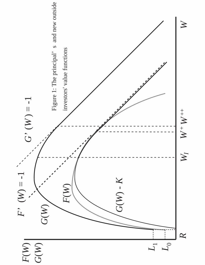
WR

F(W

)G

(W) LL 01

IW

+W

++W

G’(

W) =

-1(

F’W

) = -1

G(W

) F(W

)

G(W

) - K

Figu

re 1

: The

prin

cipa

l’s

and

new

out

side

inve

stor

s' va

lue

func

tions