MANGEMENT OF TURF IRRIGATION SYSTEM UNDER USING

741

14th

Conf. Agric. Develop. Res., Fac. of Agric., Ain Shams Univ., March, 2019, Cairo, Egypt

Special Issue, 27(1), 147 - 160, 2019 Website: http://strategy-plan.asu.edu.eg/AUJASCI/

MANGEMENT OF TURF IRRIGATION SYSTEM UNDER USING

GRAY WATER

[14] Shimaa, E. Abd Elfattah, Abdel-Aziz, A.A. and El-Bagoury K.F.

Agric. Engineering Dept., Fac. of Agric., Ain Shams Univ., P.O. Box 68 Hadyek Shoubra 11241, Cairo, Egypt

*Corresponding author: [email protected]

Received 10 February, 2019, Accepted 5 March, 2019

ABSTRACT

This research amid to obtain identify the effect

of low-quality water (gray water) (reused water

after its nomination in the special filtration stations)

on the performance analysis of the turf irrigation

system. The Experiment was carried out at EL-

Rhap site, the area under investigation was 450

m², it was divided into 6 plots, and the geometrical

has 5 m × 15 m. Investigated variables were gray

water and tap water plots were; have been while

the investigated parameter was the percentage of

the applied amounts of irrigation water with a per-

cent of 100%; 85%; 75%. The response of plant

growth landscaping parameters due to irrigation

water types were color, length, density and its cov-

erage on the after heads, the effect of gray water

and fresh water on the turf irrigation system was

compared through the study of (uniformity, Surface

roughness, Clogging ratio, flow, pressure), of

sprinklers during same the irrigation period. Re-

sults of the applied could be summarized as fol-

lowed.

The Accumulative clogging ratio by using gray

water was (1.50 – 1.56 – 1.6) % and tap water was

(1.22 – 1.25 – 1.28) % at (100% - 85% - 75%) of

quantity the water required for the plant. Illustrates

in tap water turf quality rate was (8.50 – 8.00 –

8.00) for color, very good quality rate was (8.00 –

8.00 – 7.50) for density also very good ground

cover quality rate was (8.00 – 7.50 -7.50). Mean-

while, illustrates in gray water turf quality rate was

(8.50 – 8.50 – 8.00) for color, very good quality

rate was (8.50 – 8.00 – 8.00) for density also very

good ground cover quality rate was (8.00 – 8.00 –

7.50) at (100% - 85% - 75%) of quantity the water

required for the plant. Surface roughness in the

main irrigation lines was measured after the use of

gray water and tap water. The erosion was (17.93–

65.35) Mm and the sediments were (15.48 –

58.22) Mm in gray while the erosion of tap water

was (10.45– 34.89) Mm and the sediments were

(9.06– 45.22) Mm.

Keywords: sprinkler system, gray water, land-

scape, turf grasses.

INTRODUCTION

Insufficient water supply is as yet one of the

major challenges in developing countries specially

arid and semi-arid condition. The Joint Monitoring

Programmed (JMP) for Water Supply and Sanita-

tion, implemented by the World Health Organiza-

tion (WHO) and UNICEF, reports that 783 million

people in the world (11% of the total population)

have no entrance to safe water, 84% of whom live

in rural areas. Around 187 million people use sur-

face water for drinking purposes; 94% of them are

rural inhabitants and they are concentrated in sub-

Saharan Africa (Sorlini et al 2013). The increased

water use is largely for landscape irrigation. There-

fore, irrigating landscapes with reclaimed water

can conserve tremendous amounts of fresh water.

Reclaimed water and other non-potable waters

have been used for decades for irrigating field

crops and landscapes such as golf courses, land-

scapes, and parks in many areas of the United

States (Pedrero et al 2010)

Gray water signifies wastewater that incorpo-

rates water from showers, showers, hand bowls,

clothes washers, dishwashers, and kitchen sinks,

yet rejects streams from toilets. A few creators

avoid kitchen wastewater from the other Gray wa-

ter streams. Wastewater from the washroom, in-

148 Shimaa Abd Elfattah, Abdel-Aziz and El-Bagoury

AUJAS, Ain Shams Univ., Cairo, Egypt, Special Issue, 27(1), 2019

cluding showers and tubs, is named light dark wa-

ter. Gray water that incorporates increasingly taint-

ed waste and from clothing offices, dishwashers

and, in a few occasions, kitchen sinks is called dull

dark Gray water (Albalawneh and Chang, 2015).

However, municipalities in the southwest have

encouraged the use of reclaimed water for land-

scape irrigation, because municipal water con-

sumption increases two- to twofold in summer

months compared with the winter season.

Turf grass lawns are now a central part of ur-

banized landscapes throughout North America. It

is estimated that total turf grass area, including

residential, commercial, and institutional lawns,

golf courses, Estimated 163,800 km2 in the U.S.,

and this area is expanding because of rapid urban-

ization. In Ohio, there was nearly 0.97 million ha of

turf in 1989. With highly developed root system

and dense shoots above ground, turf grass pro-

vides many environmental benefits, including soil

erosion control, water runoff and leaching reduc-

tion, contributing to carbon sequestration, moderat-

ing temperature, lessening noise, glare, and visual

pollution .often schedule -based applications of

water-soluble fertilizers and pesticides. (Cheng et

al 2008)

Irrigation from a pop-up sprinkler system has

become the accepted practice for irrigating turf

grasses. Pop-up systems can provide high-quality

turf and can also help conserve water if they pro-

vide uniform and efficient irrigation. However, An

efficient irrigation system avoids unnecessary

losses due to wind drift, surface runoff, deep per-

colation, and evaporation from standing water,

which occurs when application rates do not match

infiltration rates or the soil water-holding capacity.

To ensure uniform irrigation and water spray pat-

terns that match the shape of the area, equal con-

sideration must be given to the hydraulics( water

pressure and flow, pipe sizing) and to sprinkler

head configuration (triangular vs. square configura-

tion ), spacing (head to head), and nozzle selec-

tion. In a rectangular lawn, for example, nozzle

sizes should be "matched" so that corner sprin-

klers(which cover a 90o arc) and edge sprinklers

(which cover a 180o arc) have stream rates that

are 25% and half separately, of full circle sprinklers

(which cover a360o arc). (Leinauer and Smeal,

2012)

Water management includes using the perfect

amount of water, in the right place, at the right

time. Using a water budget program, whether it is

on the computer or a simple hand written tracking

sheet is an excellent way to make sure the amount

of water you’re using is within the budget for a par-

ticular site. (Juan G, 2014)

The objectives of this study are

1. The aim of this study is to know the effect of

using gray water on turf grass and on the irri-

gation network, evaluate amounts of irrigation

water, which can be provided using schedul-

ing system.

2. Study the effect of gray water on the network

distributers (sprinkler) such as (pressure- flow

- roughness - clogging radtios ..... etc) .

MATERIALS AND METHODS

Materials

* In this experiment, Gray water and fresh water

used to identify the effect of them on the turf grass

and the sprinkler irrigation network.

Experiment Location

The experiment was conducted Al Rehab Gate

6, Cairo at 30°3'13"N 31°29'26"E

Soil properties and irrigation water analyses

Samples of representative soil were collected

from different parts of the experimental site. The

similar depths of the soil samples were mixed thor-

oughly and a composite sample were taken for

each depth for different analyses. Some of the

physical and chemical properties of the experi-

mental soil as show in Table (1).

Table 1. Some soil properties of AL-Rhap site

when using gray water.

Soil properties parameter Valve

Soil-mechanical

Analysis and

Hydro-physical.

As (g/cm3) 1.37

FC (%) 11.24

WP (%) 6.44

AW (%) 4.80

Coarse Sand 50.32

Fine Sand 46.62

Silt + Clay 3.06

Organic Mater (%) 2.34

pH 7.5

EC (ds/m) 1.45

F.C: Field capacity %, AW: Available water %,

As: apparently density (g/cm3).

Management of turf irrigation system under using gray water


149

Chemical and Biological analyses of irrigation

water were carried out by using the standard

methods and presented in Table (2). Escherichia

coli (E. coli) were used as organism indicator to

determine the total numbers' of pathogens in gray

water, according to (Eklund and Tegelberg,

2010).

Table 2. Some biological characteristics for gray

water

con-

tent

TPC TCC FC

C

B.

C

ylo-

cocaus

TF

C

c/w/g 55×1

04

28×

10

0 0 20×10 .02

TPC: Total bacteria count (c/w/g),

TCC: Total coliform count (c/w/g),

FCC: Faecal coliform count (c/w/g),

B.C: Bacillus ceruss (c/w/g),

Staph: Staphylococcus(c/w/g),

TFC: Total fungi count (c/w/g).

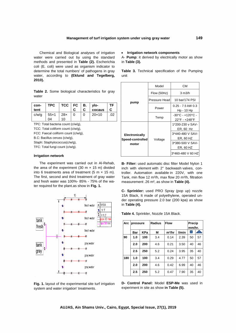
Irrigation network

The experiment was carried out in Al-Rehab,

the area of the experiment (30 m × 15 m) divided

into 6 treatments area of treatment (5 m × 15 m).

The first, second and third treatment of gray water

and fresh water was 100%- 85% - 75% of the wa-

ter required for the plant.as show in Fig. 1.

Fig. 1. layout of the experimental site turf irrigation

system and water irrigation' treatments.

Irrigation network components

A- Pump: it derived by electrically motor as show

in Table (3).

Table 3. Technical specification of the Pumping

unit

CM Model

pump

3 m3/h Flow (50Hz)

10 bar/174 PSI Pressure Head

0.25 - 7.5 kW 0.3

Hp - 10 Hp Power

-30°C - +120°C -

22°F - +248°F Temp

1*200-230 v SAV-

ER, 60 Hz

Voltage

Electronically

Speed-controlled

motor

3*440-480 V SAV-

ER, 60 HZ

3*380-500 V SAV-

ER, 60 HZ

3*460-480 V 60 HZ

B- Filter: used automatic disc filter Model Nylon 1

inch with element with 2" backwash valves, con-

troller. Automation available in 220V, with one

Tank, min flow 12 m³/h, max flow 20 m³/h, filtration

measurement .26 m², as show in Table (4).

C- Sprinkler: used PRO Spray (pop up) nozzle

15A Black, It made of polyethylene, operated un-

der operating pressure 2.0 bar (200 kpa) as show

in Table (4).

Table 4. Sprinkler, Nozzle 15A Black.

Arc pressure Radius Flow Precip

mm/hr.

Bar KPa M m³/hr l/min

90 1.0 100 3.4 0.14 2.39 50 57

2.0 200 4.6 0.21 3.50 40 46

2.5 250 5.2 0.24 3.95 35 40

180 1.0 100 3.4 0.29 4.77 50 57

2.0 200 4.6 0.42 6.99 40 46

2.5 250 5.2 0.47 7.90 35 40

D- Control Panel: Model ESP-Me was used in

experiment in site as show in Table (5).



Table 5. Technical specifications of the Control

panel ESP-Me

Support Stations 22 stations

memory Permanently (100 year)

Station timing from 1 minute to 6 hours

Seasonal adjust 5% to 200%

Maximum temp 149° F (65 ° C)

Features Delay Watering up to 14 days.

Manual Watering option by

program or station

Adjustable delay between

valves (default set to 0(

Upgradeable for Wi-Fi-based

remote monitoring and control

viaiOS and Internet-based

weather information can be

used to make daily

Internet-based weather infor-

mation can be used to make

daily

Description of landscaping plants

Experiment was conducted on an herbaceous

plant Paspalm 10, it was green, The width was

within 3-4 mm and the length was within 1 cm, It

can tolerate high salinity levels In 8,000 - 10000

ppm and, It bears high temperatures, Bear with

bad ventilation, Resistant to pests and insects, It

grows in an average state in the shade, it will en-

dure running and walking. Irrigation water require-

ment values were presented in Results.

Fertilization: The landscape are fertilized, main-

tained and irrigation as show in Table (6).

Table 6. Periodic maintenance of the surface .

Activity April May June

Cut plant 4/month 4/month 4/month

Challenges 4/month 4/month 4/month

Remove the

strange

4/month 4/month 4/month

Fertilization Urea Micro elements Urea

Irrigation Daily Daily Daily

Calculated and Measurements experiment

A- Climate data in experiment

The data were taken from the meteorological

station as show in Table (7).

Table 7. Climate data of experiment location in

ElRhap

Month

Min

Temp

Max

Temp Humidity Wind Sun Red Eto

c C % Km/

day hours

Mj/m2/

day

mm/

day

April 14.70 32.00 32.1 397.4 9.71 23.26 7.03

May 17.50 34.20 29.10 371.5 10.69 25.81 8.44

June 20.40 34.40 31.10 319.7 11.67 27.76 9.06

Temp. Min: Minimum temperature in C;

Temp. Max: Maximum temperature in C;

Eto : Value of evaporation, Sun shine fraction in percentage;

Wind speed at 2 meter above the surface in m/s and Eto = Refer-

ence evapotranspiration in mm/d (FAO, 2001).

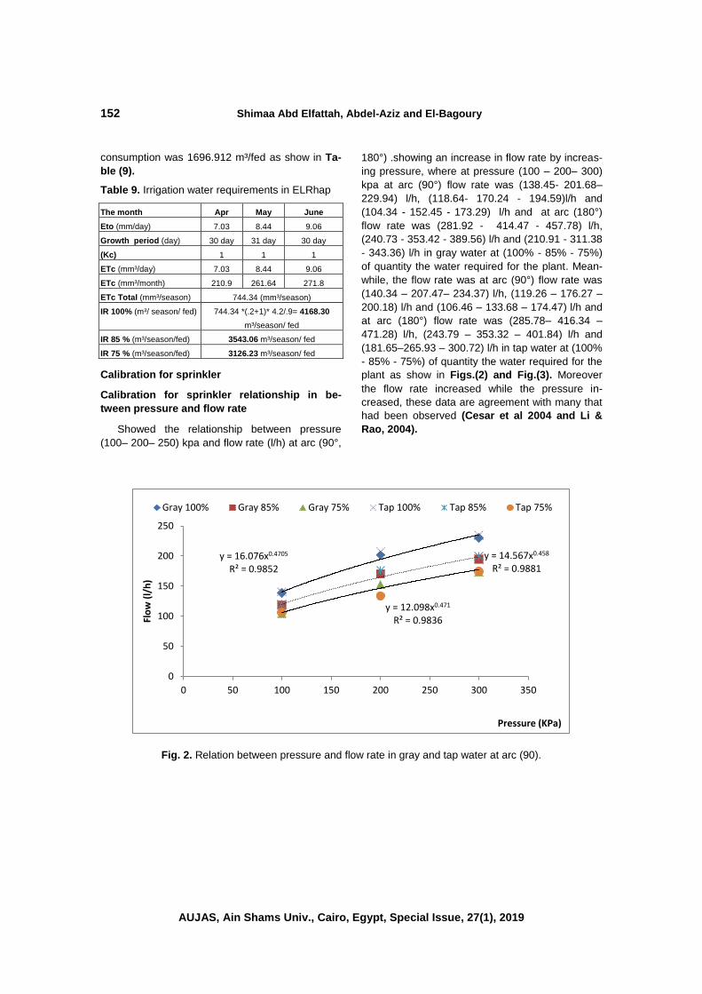
B- Calibration sprinklers

Show that the relationship between pressure

(kpa) and flow rate (l / h). When the pressure is

150, 200, 250 when the bow (90) and arc (180) in

AL-Rhap when using fresh water and gray.

C- The validity of irrigation water on turf

grasses.

Measuring the effect of gray water and fresh

water on turf grasses in AL-Rhap use on the plant

in terms of color, density, and ground cover as

show in Table (8) Indicates turf quality index and

represents color, density, and ground .

Table 8. Cover percent for lawn plant (paspalum).

(Khaseeva, 2013)

Type of turf Color Density Ground

cover

Paspalum 0-9 0-9 1-9

E- Measurement of surface roughness

Pipes samples were taken from different parts

of the network (main lines - sub main lines - mani-

fold lines), five grinding operations were carried out

at the cutting site to study surface roughness after

3 months. The samples were placed under elec-

tronic microscope with zoom (1:1000), to study the

roughness on part of the circumference of the

pipes by a distance, in the production Laboratory

of Faculty of Engineering.



151

Methods

Estimating water needs for landscape plantings

Costello et al (1993) derived plant water re-

quirement on ETo as a reference to a cool-season

grass species with a specified height (typically 7-15

cm tall) under particular growing conditions, this

reference must be adjusted to better fit the plant

water requirement of a specific plant species in the

landscape setting. The landscape coefficient Kl is

used to adjust ETo to determine the plant water

requirement (PWR) of a specific plat species.

Kl = Ks × Kmc × Kd …………………..(1)

Where:

Kl = Landscape coefficient (dimensionless).

Kmc = Adjustment factor for microclimate influ-

ences upon the planting (dimensionless)

Ks = Adjustment factor representing character-

istics for a particular plant species (dimensionless).

Kd= Adjustment factor for plat density (dimen-

sionless).

Awady et al. (2003) used two formulas to es-

timate water needs for landscape plantings:

The landscape evapotranspiration formula

and,

The landscape coefficient formula.

Water needs of landscape plantings can be es-

timated using the landscape evapotranspiration

formula:

ETl = Kl × ETo ………………………………(2)

Estimating of irrigation requirements

From the following equation (Abrol et al1988)

( )

( )

Where

IR = irrigation requirement, L/day; LR=

Leaching requirement, (20%);

Ea = Irrigation uniformity (68%) (Measured in

the field); A= Area of tree (m2)

;

ETcrop = Potential Evaporation-Transpiration.

The Flow rate

Measure the water collected from sprinkler

nozzle using a 1000 ml graduated cylinder. Deter-

mine the flow rate from following equation

(Melvyn, 1983).

( )

Where:

Q = the flow rate of sprinkler in m3/h.

V = the collecting water volume in m3.

T = time of collecting water in h.

3-2-4- Sensitive for clogging

Emitter nozzles are designed with diameter

ranging from (0.25 mm- 2.5 mm) and this cause in

clogging. (Al-Amoud. 1997)

Following formula was used to calculate clog-

ging ratio.

Clogging ratio (

) ( )

Where:

Q1= Average flow rate at start up operating

(l/h).

Q2= Average flow rate at the end operating

(l/h).

Distribution uniformity

Plastic catch cans 95 mm diameter; 120 mm

height were located under impact Sprinkler in a

quarter circle. The catch cans were distributed

according to (ASAE Standard, 2001). Fig.8: shape

of Regularity of Distribution:

{ |־ |∑

־ } ( )

Where:

CU = the Christiansen's coefficient of uniformity

in %.

x = Numerical deviation of individual observa-

tion from average application rate, mm.

x־ = mean of collectors amount in mm.

n = number of catch cans.

Precipitation rate

The precipitation rate of sprinkler was calculat-

ed by the following formula (James, 1988):

( )

Where:

Pr= the precipitation rate in mm / h.

Q = the flow rate of sprinkler in L/ min.

a= the wetted area of sprinkler in m2.

K = unit constant.

Irrigation schedule when using water

The Irrigation scheduling process was started a

week after the primary irrigation of cultivation. Af-

terwards, the irrigation was given approximately

every day, in April, May and June. The total water



consumption was 1696.912 m³/fed as show in Ta-

ble (9).

Table 9. Irrigation water requirements in ELRhap

June May Apr The month

9.06 8.44 7.03 Eto (mm/day)

30 day 31 day 30 day Growth period (day)

1 1 1 (Kc)

9.06 8.44 7.03 ETc (mm³/day)

271.8 261.64 210.9 ETc (mm³/month)

744.34 (mm³/season) ETc Total (mm³/season)

744.34 *(.2+1)* 4.2/.9= 4168.30

m³/season/ fed

IR 100% (m³/ season/ fed)

3543.06 m³/season/ fed IR 85 % (m³/season/fed)

3126.23 m³/season/ fed IR 75 % (m³/season/fed)

Calibration for sprinkler

Calibration for sprinkler relationship in be-

tween pressure and flow rate

Showed the relationship between pressure

(100– 200– 250) kpa and flow rate (l/h) at arc (90°,

180°) .showing an increase in flow rate by increas-

ing pressure, where at pressure (100 – 200– 300)

kpa at arc (90°) flow rate was (138.45- 201.68–

229.94) l/h, (118.64- 170.24 - 194.59)l/h and

(104.34 - 152.45 - 173.29) l/h and at arc (180°)

flow rate was (281.92 - 414.47 - 457.78) l/h,

(240.73 - 353.42 - 389.56) l/h and (210.91 - 311.38

- 343.36) l/h in gray water at (100% - 85% - 75%)

of quantity the water required for the plant. Mean-

while, the flow rate was at arc (90°) flow rate was

(140.34 – 207.47– 234.37) l/h, (119.26 – 176.27 –

200.18) l/h and (106.46 – 133.68 – 174.47) l/h and

at arc (180°) flow rate was (285.78– 416.34 –

471.28) l/h, (243.79 – 353.32 – 401.84) l/h and

(181.65–265.93 – 300.72) l/h in tap water at (100%

- 85% - 75%) of quantity the water required for the

plant as show in Figs.(2) and Fig.(3). Moreover

the flow rate increased while the pressure in-

creased, these data are agreement with many that

had been observed (Cesar et al 2004 and Li &

Rao, 2004).

Fig. 2. Relation between pressure and flow rate in gray and tap water at arc (90).

y = 16.076x0.4705 R² = 0.9852

y = 14.567x0.458 R² = 0.9881

y = 12.098x0.471 R² = 0.9836

0

50

100

150

200

250

0 50 100 150 200 250 300 350

Flo

w (

l/h

)

Pressure (KPa)

Gray 100% Gray 85% Gray 75% Tap 100% Tap 85% Tap 75%



153

Fig. 3. Relation between pressure and flow rate in gray and tap water at arc (180).

Calibration for sprinkler in relationship be-

tween flow rate and time

The relationship between pressure flow rate

(l/h) and time (3 months) by using gray water and

tap water .As show in Figs.(4) and Fig.(5), Show-

ing decrease in flow rate by the time, where at

pressure (200 kpa) at arc (90° - 180°), flow rate at

arc (90°) was (204.83– 195.24.18- 187.68) l/h,

(174.28– 169.46 - 162.28) l/h and (154.16- 148.85

- 143.21) l/h, at arc (180°) (414.24 - 404.93-

396.00) l/h, (352.83 - 342.92 - 340.23) l/h and

(308.76 - 300.28 - 294.75) l/h using gray water.

Meanwhile, the flow rate in arc (90°) was (208.37 -

206.90 - 206.23) l/h, (176.15 – 174.95 - 174.01) l/h

and (156.34 - 155.36 - 154.25) l/h, at arc (180°)

(417.37 - 413.46 - 413.29) l/h, (354.34 - 352.21-

350.78) l/h and (310.06 - 309.08 - 305.33) l/h using

tap water. At (100% - 85% - 75%) of quantity the

water required for the plant .Hence, that the per-

formance rate for sprinkler nozzles by using tap

water was better than the gray water.

Fig. 4. Evaluate between time and flow rate in gray water and tap water at arc (90°).

y = 35.581x0.4536 R² = 0.9686

y = 30.811x0.4506 R² = 0.9676

y = 26.3x0.4564 R² = 0.967

050

100150200250300350400450500

0 50 100 150 200 250 300 350

Flo

w (

l/h

)

Pressure (kPa)

Gray 100% Gray 85% Gray 75% Tap 100% Tap 85% Tap 75%

0

50

100

150

200

250

April May June

Flo

w (

l/h

)

Months

Tap 100% Tap 85% Tap 75%

Gray 100% Gray 85% Gray 75%



Fig. 5. Evaluate between time and flow rate in gray water and tap water at arc (180°).

The validity of irrigation water on turf grasses.

Show the measuring the effect of tap water and

gray water use on the plant in terms of color, den-

sity and ground cover at (100% - 85% - 75%) of

quantity the water required for the plant. illustrates

in tap water turf quality rate was (8.50 – 8.00 –

8.00) for color, very good quality rate was (8.00 –

8.00 – 7.50) for density also very good ground

cover quality rate was (8.00 – 7.50 -7.50). Mean-

while, illustrates in gray water turf quality rate was

(8.50 – 8.50 – 8.00) for color, very good quality

rate was (8.50 – 8.00 – 8.00) for density also very

good ground cover quality rate was (8.00 – 8.00 –

7.50) at (100% - 85% - 75%) of quantity the water

required for the plant.

Results are also in agreement with (pinto et al

2010) results who reported that no significant dif-

ference was observed in silver beet growth over 60

days when it was irrigated with fresh water and

gray water. The data suggest that small difference

may be observed in plant growth when irrigated

with gray water depending on soil type and plant

specific factors.4-1-1-Growth measurements for

length, dentistry, color for plant the existence of

spaces.

Clogging ratio

The Accumulative clogging ratio by using gray

water was (1.50 – 1.56 – 1.6) % and tap water was

(1.22 – 1.25 – 1.28) % at (100% - 85% - 75%) of

quantity the water required for the plant as show in

fig. (6). Hence, that the accumulative clogging ratio

by using gray water higher than using tap water

and agree with many author.

The weight of the impurities was measured

from network irrigation every month for three

month which was in tap water was (2.64 – 2.96 –

3.13) g/m², (2.25 – 2.66 – 2.54) g/m² and (2.04 –

2.31 – 2.28) g/m² as show in fig.(10). The impuri-

ties was measured in gray water (3.92 – 4.15 –

4.16) g/m², (3.32 - 3.21 – 3.28) g/m² and (3.10 –

2.97 – 2.93) g/m² at (100% - 85% - 75%) of quanti-

ty the water required for the plant as show in Fig.

(7) and Fig.(8).

0

50

100

150

200

250

300

350

400

450

April May June

Flo

w (

l/h

)

months


Tap 100% Tap 85% Tap 75%



155

Fig. 6. The Accumulative clogging ratio by using gray water and tap water.

Fig. 7. Measurement of impurities on the irrigation with tap water.

Fig. 8. Measurement of impurities on the irrigation with gray water.

0

0.2

0.4

0.6

0.8

1

1.2

1.4

1.6

1.8

April May June

Clo

ggin

g ra

tio

(%

)

Months

Gray water Tap water2

0

0.5

1

1.5

2

2.5

3

3.5

April May June

The

imp

uri

tiie

s (g

/m²)

Months

Tap 100% Tap 85% Tap 50%

0

0.5

1

1.5

2

2.5

3

3.5

4

4.5

April May June

The

imp

uri

tie

s (g

/m²)

Months




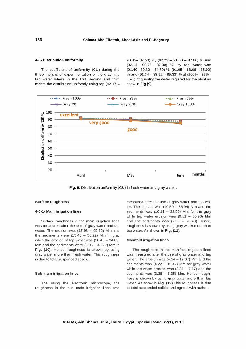
4-5- Distribution uniformity

The coefficient of uniformity (CU) during the

three months of experimentation of the gray and

tap water where in the first, second and third

month the distribution uniformly using tap (92.17 –

90.85– 87.50) %, (92.23 – 91.00 – 87.66) % and

(92.14– 90.75– 87.00) % ,by tap water was

(91.40– 89.80 – 84.70) %, (91.95 – 88.66 – 85.90)

% and (91.34 – 88.52 – 85.33) % at (100% - 85% -

75%) of quantity the water required for the plant as

show in Fig.(9).

Fig. 9. Distribution uniformity (CU) in fresh water and gray water .

Surface roughness

4-6-1- Main irrigation lines

Surface roughness in the main irrigation lines

was measured after the use of gray water and tap

water. The erosion was (17.93 – 65.35) Mm and

the sediments were (15.48 – 58.22) Mm in gray

while the erosion of tap water was (10.45 – 34.89)

Mm and the sediments were (9.06 – 45.22) Mm in

Fig. (10). Hence, roughness is shown by using

gray water more than fresh water. This roughness

is due to total suspended solids.

Sub main irrigation lines

The using the electronic microscope, the

roughness in the sub main irrigation lines was

measured after the use of gray water and tap wa-

ter. The erosion was (10.50 – 35.94) Mm and the

sediments was (10.11 – 32.55) Mm for the gray

while tap water erosion was (9.11 – 30.93) Mm

and the sediments was (7.50 – 20.48) Hence,

roughness is shown by using gray water more than

tap water. As shown in Fig. (11).

Manifold irrigation lines

The roughness in the manifold irrigation lines

was measured after the use of gray water and tap

water. The erosion was (4.54 – 12.37) Mm and the

sediments was (4.22 – 12.47) Mm for gray water

while tap water erosion was (3.36 – 7.57) and the

sediments was (3.36 – 6.35) Mm. Hence, rough-

ness is shown by using gray water more than tap

water. As show in Fig. (12).This roughness is due

to total suspended solids, and agrees with author.

20

30

40

50

60

70

80

90

100

April May June

Dis

trib

uti

on

un

ifo

rmit

y (C

U)

%.

months

Fresh 100% Fresh 85% Fresh 75%




157

Fig. 10. Surface roughness for main lines by using tap and gray water.

Fig.11. Surface roughness for sub main lines by using tap and gray water .

Fig. 12. Surface roughness for manifold lines by using tap and gray water .

-80

-60

-40

-20

0

20

40

60

80

0 300 600 900 1200 1500 1800 2100 2400 2700 3000 3300

Surf

ace

ro

ugh

ne

ss (

Mm

)

length (Mm)

Gray water Tap water

-80

-60

-40

-20

0

20

40

60

80

0 300 600 900 1200 1500 1800 2100 2400 2700 3000 3300

Surf

ace

ro

ugh

ne

ss (

Mm

)

Length (Mm)


-80

-60

-40

-20

0

20

40

60

80

0 300 600 900 1200 1500 1800 2100 2400 2700 3000 3300

Surf

ace

ro

ugh

ne

ss (

Mm

)

Lenght (Mm)


Erosion (Mm)

Sediments (Mm)



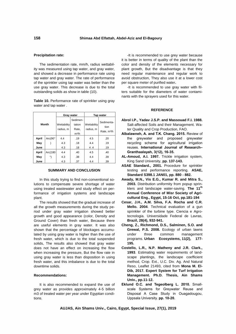
Precipitation rate:

The sedimentation rate, mm/h, radius wettabil-

ity was measured using tap water, and gray water,

and showed a decrease in performance rate using

tap water and gray water. The rate of performance

of the sprinkler using tap water was better than the

use gray water. This decrease is due to the total

outstanding solids as show in table (10).

Table 10. Performance rate of sprinkler using gray

water and tap water .

Month


Wettability

radius, m

Sedimen-

tation

Rate,

m³/h

Wettability

radius, m

Sedimenta-

tion

Rate, m³/h

April Arc(90°

)

4.4 .19 4.5 .20

May 4.3 .18 4.4 .19

June 4.3 .18 4 .4 .19

April Arc(180

°)

4.4 .40 4.5 .40

May 4.3 .38 4.4 .39

June 4.3 .37 4.4 .39

SUMMARY AND CONCLUSION

In this study trying to find non-conventional so-

lutions to compensate severe shortage of water

using treated wastewater and study effect on per-

formance of irrigation systems and landscape

plant.

The results showed that the gradual increase of

all the growth measurements during the study pe-

riod under gray water irrigation showed better

growth and good appearance (color, Density and

Ground Cover) than fresh water, Because there

are useful elements in gray water. It was also

shown that the percentage of blockages accumu-

lated by using gray water is higher than the use of

fresh water, which is due to the total suspended

solids, The results also showed that gray water

does not have an effect on increasing the flow

when increasing the pressure, But the flow rate in

using gray water is less than disposition in using

fresh water, and this imbalance is due to the total

downtime solids.

Recommendations:

It is also recommended to expand the use of

grey water as provides approximately 4-5 billion

m3 of treated water per year under Egyptian condi-

tions.

-It is recommended to use grey water because

it is better in terms of quality of the plant than the

color and density of the elements necessary for

plant growth, But the disadvantage is that they

need regular maintenance and regular work to

avoid obstruction, They also use it at a lower cost

per square meter of purified water.

-It is recommended to use gray water with fil-

ters suitable for the diameters of water contami-

nants with the sprayers used for this water.

REFERENCE

Abrol I.P., Yadav J.S.P. and Massouad F.I. 1988.

Salt-affected Soils and their Management. Wa-

ter Quality and Crop Production, FAO.

Albalawneh, A. and T.K. Chang. 2015. Review of

the greywater and proposed greywater

recycling scheme for agricultural irrigation

reuses. International Journal of Research–

Granthaalayah, 3(12), 16-35.

AL-Amoud, A.I. 1997. Trickle irrigation system,

King Sand University, pp. 137-143.

ASAE Standard., 2001. Procedure for sprinkler

testing and performance reporting. ASAE,

Standard S398.1 JAN01, pp. 880 - 882.

Awady, M.N., Vis E.G., Kumar R. and Mitra S.,

2003. Distribution uniformity from popup sprin-

klers and landscape water-saving. The 11th

Annual Conference of Misr Society of Agri-

cultural Eng., Egypt, 15-16 Oct, pp.181-194

Cesar, J.H., A.M. Silva, F.A. Rocha and C.R.

Mello. 2004. Technical evaluation of a gun

sprinkler of the turbine type. Ciencia e Agro-

tecnologia. Universidade Federal de Lavras,

Brazil, 28(4), 932-941.

Cheng, Z., Richmond, D.S., Salminen, S.O. and

Grewal, P.S. 2008. Ecology of urban lawns

under three common management

programs. Urban Ecosystems, 11(2), 177-

195.

Costello, L.R., N.P. Matheny and J.R. Clark.,

1993. Estimating water requirements of land-

scape plantings, the landscape coefficient

method, Crop. Ext., U.C. Div. Ag. And Natural

Reso, Leaflet 21493, cited from Mona M. El-

Dib, 2017. Expert System for Turf Irrigation

Management. Ph.D. Thesis, Ain Shams

Univ., pp.11-12.

Eklund O.C. and Tegeolberg L. 2010. Small-

scale Systems for Greywater Reuse and

Disposal A Case Study in Ouagadougou,

Uppsala University. pp. 10-20.



159

FAO, 2001. FAO AQUASTAT. FAO’s Information

System on water and Agriculture: climate In-

formation tool. AQUASTAT climatemcharacter-

istics.http://www.fao.org/nr/water/aquastat/gis.

James, L.G. 1988. Principles of farm irrigation

system design. New York: John Wiley and

Sons. 545 p.

Juan G. 2014. Water quality and water-use effi-

ciency in landscapes, a training manual devel-

oped for landscape maintenance, personnel

Water Wise Consulting, Inc. 300 S. Raymond

Ave., Suite 20 Pasadena, pp. 626-793.

Khaseeve, K.A., 2013. Evaluation of turf quality

for cool season species and cultivars, Russian

St. Ag.U., MOSCOW, Russia, 92(8),115-129.

Leinauer, B. and Smeal, D. 2012. Turfgrass

Irrigation. Circular 660. NMSU and the U.S.

Dep. of Ag. Cooperating, 12p.

Li, J. and M. Rao. 2004. Crop yield as affected by

uniformity of sprinkler irrigation system. Agri-

cultural Eng. Int. The CIGR J. Sci. Res. Dev.

111 p.

Melvyn, K., 1983. Sprinkler irrigation, equipment

and practice. Batsford Academic and Educa-

tional, London. 120 p., cited from Doaa M.

Sayed 2016, Effect of some Engineering

Factors of Sprinkler Irrigation on Sprinkler

Performance, M.Sc., Thesis, Ain Shams

Univ., pp. 21-22.

Pedrero, F.I., Kalavrouziotis J.J. and

Koukoulakis P.T. 2010. Use of treated

municipal. wastewater in irrigated agriculture-

Review of some practices in Spain and Greece.

Agricultural Water Management, 97(9), 1233-

1241

Pinto, U; B. Maheshwari and H. Grewal., 2010.

Effects of Gray water irrigation on plant growyh,

water use and soil properties. Resources,

Cons and Recy. 54(7), 429-435.

Sorlini, S., Palazzini, D., Sieliechi, J.M. and

Ngassoum, M.B., 2013. Assessment of

physical-chemical drinking water quality in the

Logone Valley (Chad-Cameroon). Sustain-

ability, 5(7), 3060-3076.

لتنمية الزراعية،لبحوث االمؤتمر الرابع عشر

، القاهرة، مصر9102، مارس كلية الزراعة، جامعة عين شمس 9102، 061 - 042، مارسعدد خاص (،0) ددع (،92)جلدم

plan.asu.edu.eg/AUJASCI/-http://strategyWebsite: 761

]04[

*Corresponding author: [email protected]

Received 10 February, 2019, Accepted 5 March, 2019

.

Documents

MANGEMENT OF TURF IRRIGATION SYSTEM UNDER USING