Mantle Shear-Wave Tomography and the Fate of …rcoe/eart206/Grand_S-waveTomog_PhilTrans...Mantle shear-wave tomography to 200 km. Our approach is to examine all tangential-component

Mantle Shear-Wave Tomography and the Fate of Subducted SlabsAuthor(s): Steven P. GrandSource: Philosophical Transactions: Mathematical, Physical and Engineering Sciences, Vol. 360,No. 1800, Chemical Reservoirs and Convection in the Earth's Mantle (Nov. 15, 2002), pp. 2475-2491Published by: The Royal SocietyStable URL: http://www.jstor.org/stable/3558906Accessed: 14/01/2010 18:04

Your use of the JSTOR archive indicates your acceptance of JSTOR's Terms and Conditions of Use, available athttp://www.jstor.org/page/info/about/policies/terms.jsp. JSTOR's Terms and Conditions of Use provides, in part, that unlessyou have obtained prior permission, you may not download an entire issue of a journal or multiple copies of articles, and youmay use content in the JSTOR archive only for your personal, non-commercial use.

Please contact the publisher regarding any further use of this work. Publisher contact information may be obtained athttp://www.jstor.org/action/showPublisher?publisherCode=rsl.

Each copy of any part of a JSTOR transmission must contain the same copyright notice that appears on the screen or printedpage of such transmission.

JSTOR is a not-for-profit service that helps scholars, researchers, and students discover, use, and build upon a wide range ofcontent in a trusted digital archive. We use information technology and tools to increase productivity and facilitate new formsof scholarship. For more information about JSTOR, please contact [email protected].

The Royal Society is collaborating with JSTOR to digitize, preserve and extend access to PhilosophicalTransactions: Mathematical, Physical and Engineering Sciences.

http://www.jstor.org

http://www.jstor.org/stable/3558906?origin=JSTOR-pdf

http://www.jstor.org/page/info/about/policies/terms.jsp

http://www.jstor.org/action/showPublisher?publisherCode=rsl

tH THE ROYAL 10.1098/rsta.2002.1077 *i!S SOCIETY

Mantle shear-wave tomography and the fate of subducted slabs

BY STEVEN P. GRAND

Department of Geological Sciences, University of Texas at Austin, Austin, TX 78712-1101, USA

Published online 6 September 2002

A new seismic model of the three-dimensional variation in shear velocity throughout the Earth's mantle is presented. The model is derived entirely from shear bodywave travel times. Multibounce shear waves, core-reflected waves and SKS and SKKS waves that travel through the core are used in the analysis. A unique aspect of the dataset used in this study is the use of bodywaves that turn at shallow depths in the mantle, some of which are triplicated. The new model is compared with other global shear models. Although competing models show significant variations, several large-scale structures are common to most of the models. The high-velocity anomalies are mostly associated with subduction zones. In some regions the anomalies only extend into the shallow lower mantle, whereas in other regions tabular high- velocity structures seem to extend to the deepest mantle. The base of the mantle shows long-wavelength high-velocity zones also associated with subduction zones. The heterogeneity seen in global tomography models is difficult to interpret in terms of mantle flow due to variations in structure from one subduction zone to another. The simplest interpretation of the seismic images is that slabs in general penetrate to the deepest mantle, although the flow is likely to be sporadic. The interruption in slab sinking is likely to be associated with the 660 km discontinuity.

Keywords: mantle; seismic; structure; tomography

1. Introduction

Over the past decade, global seismic tomography studies have produced consistent images of the very-large-scale seismic structure of Earth's mantle. At present, however, many of the details of tomography models differ. These differences still leave uncertain an unambiguous interpretation of the tomography results in terms of mantle flow and, by implication, the thermal and chemical structure of the mantle. Some of the differences seen in tomographic models result from the use of different datasets, whereas other differences probably result from different inversion approaches. Data supplied by the International Seismic Center (ISC) have been used by several authors to image the three-dimensional variations in compressional wave speed. Recent examples of models derived using ISC data include those by Obayashi et al. (1997), Kara- son & van der Hilst (2000), Bijwaard et al. (1998) and Zhao (2001). The primary

One contribution of 14 to a Discussion Meeting 'Chemical reservoirs and convection in the Earth's mantle'.

Phil. Trans. R. Soc. Lond. A (2002) 360, 2475-2491 ) 2002 The Royal Society 2475

S. P. Grand

data used in these studies are the travel times of direct primary (P) waves. With several million observations, the ISC P-wave data provide the highest resolution of mantle structure in regions that are well sampled by direct P-waves. In particular, subduction zones are imaged in great detail by ISC P-wave travel-time data (see, for example, Spakman et al. 1993; Widiyantoro & van der Hilst 1996 and van der Hilst 1995). A weakness of the ISC data, however, is that large regions of the upper mantle and top of the lower mantle are not well sampled by direct waves due to the distribution of receivers and earthquakes. The addition of travel times for later phases such as PP-waves, improves the coverage using ISC data, but the reported times of these phases are likely to be not as reliable as the arrival times of direct P-waves.

Three-dimensional shear-wave models of the mantle have also been produced using the ISC database (Robertson & Woodhouse 1996; Widiyantoro et al. 1998). These models suffer from the same limitations as the P-wave models with respect to data coverage. Most models of mantle shear-wave velocity structure have relied on direct analysis of seismic waveforms in one form or another. Data extracted from seismic waveforms include surface-wave dispersion and structural constraints from the split- ting of normal modes, as well as the travel times of a number of different seismic phases such as S, SS, SKS and ScS waves. Recent mantle-shear models that use various combinations of data extracted from seismic waveforms include those by Masters et al. (2000), Megnin & Romanowicz (2000), Gu et al. (2001) and Ritsema et al. (1999). Although the database derived from seismic waveforms is large and grow- ing larger, the number of observations used to constrain mantle shear-wave velocity variations is still far smaller than the ISC database provides for P-wave structure. Thus, the S-models tend to have lower resolution than the ISC-based P-models. On the other hand, the use of surface waves and multibounce seismic phases such as SS waves gives a more uniform global coverage of the mantle as well as far more information on upper-mantle seismic structure.

The models of mantle seismic structure mentioned above, as well as others, show similar large-scale structures within the mantle. High seismic velocities are found beneath shield regions to depths exceeding 200 km in most studies. Large, fast seismic anomalies are found in the transition zone, 400-660 km depth, throughout the western Pacific subduction zones. The base of the mantle is dominated by a spheri- cal harmonic degree-two pattern for shear-wave velocity with strong, slow anomalies beneath the southwestern Pacific and beneath Africa. In detail, however, seismic tomography models show differences that have led researchers to widely different views as to their implications for mantle flow. Hamilton (2002) infers that mantle flow is essentially blocked at 660 km in depth. Fukao et al. (2001) conclude that subducted slabs enter the lower mantle but are stagnant above ca. 1000 km in depth. Kellogg et al. (1999) have proposed that subducted slabs sink to deep within the lower mantle but that there is a chemically distinct layer in the lower 1000 km of the mantle, through which slabs cannot penetrate. Finally, Richards & Engebretson (1992) proposed that the D" layer at the base of the mantle may be a slab grave- yard. Part of the reason for the different views on mantle flow is the disagreement in short-wavelength features among tomography models. It is likely that, as tomography models produced through different approaches, using different data, by different researchers, converge to similar images, some of the uncertainty in how the mantle convects will decrease.

Phil. Trans. R. Soc. Lond. A (2002)

2476

Mantle shear-wave tomography

(a) s S SS

SSS

300 s I I

(b) sssss SSSSS distance: 88.8?

elocity model: TNA

S SKS

Figure 1. (a) A horizontally polarized seismogram recorded in the western United States from an earthquake that occurred in the southern Pacific Ocean. Below the seismogram is a synthetic seismogram. Numerous phases that have good matches between the synthetic and data are labelled. The large arrival at the end of the seismogram is the Love wave that consists of SSSSS and higher-order multiples of S. Part (b) shows the paths taken by the phases labelled at the top, as well as the paths of phases that interact with the core, which, although not visible in the record shown above, are seen in other seismograms used in this study.

In this paper I present a new global mantle-shear-velocity model. The model is derived using an approach different from those used in other studies. The data are also, to some extent, independent of datasets used in other published shear-velocity models. Various models are compared with the model presented in this study, and features that are common to most models I assume are robust features of the mantle. These robust features will be used to assess the pattern of downward flow in the mantle.

2. Data

The data used to derive the model presented in this paper consist of the arrival times of several different seismic phases. The approach used to measure the time information is discussed in more detail in Grand (1994). Here I will briefly review the observations used to construct the tomography model. Figure la shows an example of a


2477

S. P. Grand

Figure 2. A map showing the stations (diamonds) and earthquakes (crosses) used in this study.

Figure 3. Map of the bounce points of all multibounce shear phases used in the this study. Note the uneven sampling, with less coverage in the Southern Hemisphere.

tangential component seismogram produced by an earthquake in the southern Pacific Ocean, recorded in the western United States. Below the seismogram is a synthetic seismogram computed using the reflectivity method (Fuchs & Muller 1971). Note the excellent correlation of timing as well as waveform between the synthetic seismogram and the data. The arrivals are labelled and consist of multiple-bounce shear waves from S to SSSS and their paths through the mantle are shown in figure lb. The large unlabelled arrival at the end of the seismogram is a Love wave, although it can also be thought of as higher-order multiple-bounce shear waves that arrive at nearly the same time. Our synthetic matches the timing and shape of this arrival as well. The beginning of the Love wave is actually formed by SSSSS with a turning depth near


2478


to 200 km. Our approach is to examine all tangential-component seismograms from a particular earthquake and, with the aid of synthetic seismograms, identify clear arrivals present on the seismogram. For each identified arrival, the synthetic and datum are cross-correlated to measure an arrival time. The arrival times are then compared with predicted arrival times for a one-dimensional shear-velocity starting model. The travel-time residuals, the difference between the predicted and measured times, are the data used in the inversion. The starting model is an average of models TNA and SNA given in Grand & Helmberger (1984) for the upper mantle and PREM (Dziewonski & Anderson 1981) for the lower mantle.

The good fit between the synthetic and actual seismogram shown in figure la is not the result of the starting model being a close approximation to the actual mantle shear velocity. The seismic model used to compute the synthetic was adjusted to match the waveforms and timing of the observed seismogram. This was done for each seismogram used in the study, which had propagation paths turning within the upper mantle. The paths corresponding to observed waves are determined with respect to the adjusted model that predicts the observed waveforms, whereas the residuals are with respect to the one-dimensional starting model. The equation used to determine the residuals is

6t (sp -ss)dr + 5ts,

where 6t is the residual with respect to starting model, 6ts is the residual measured by cross-correlation using the adjusted model, s, is the slowness of the adjusted model and sp is the slowness of the starting model. The integral is along the ray path predicted by the adjusted model. The attempt here is to take advantage of classical waveform modelling (e.g. Helmberger & Engen 1974), but also to retain a simple database of paths through the mantle with a corresponding time residual associated with the path with respect to a simple one-dimensional velocity model. This approach also allows use of bodywaves that turn within the upper mantle and interact with upper-mantle discontinuities that produce complicated multiple arrivals or triplications. In many cases, the synthetics do not match the data very well. This is likely to be due to unmodelled three-dimensional variations in seismic velocity. In these cases the data were not used. The approach is discussed in detail in Grand (1994), where many examples are shown. Multiple bounce waves up to SSSSS were measured for this study.

Other phases not apparent in figure la were also used in the study. These include ScS and ScSScS waves that reflect from the core-mantle boundary measured off tangential-component seismograms. The only data measured from the radial component of seismograms were SKS and SKKS waves that propagate as S through the mantle and as compressional waves within the outer core.

The seismograms used in the study came from numerous networks. Older data used in Grand (1994) came from the World Wide Standard Seismic Network and the Canadian network. More recent data were obtained from numerous global and regional networks (IRIS GSN, GEOSCOPE, MedNet, CNSN and temporary PASS- CAL deployments). The digital data were bandpassed from 0.07 to 0.01 Hz. Figure 2 shows all the stations used, as well as the earthquakes analysed. Data were measured for 311 earthquakes, resulting in ca. 25 000 travel-time residuals with associated paths through the mantle. Earthquake locations were taken from the ISC, with the depths


2479

S. P. Grand

(a) 12-

10-

8-

2C

0

0 600 1200

depth (km)

(b) 12

10

8

6

4

2

0 600 1200 1800 2400

depth (km)

Figure 4. The root mean square (RMS) of travel-time residuals as a function of turning depth (a) in the measured data and (b) with respect to a model with lateral variations in the upper 400 km and bottom 240 km of the mantle. In (a) multibounce shear waves are included, but their residuals are divided by the number of passes each has taken through the mantle; note the large residuals for waves that sample the shallow and deep mantle of turning depth.


1800 2400 3000

3000

2480


determined by examining the time difference between S and sS in the data. Figure 3 shows the bouncepoints for multibounce arrivals measured in the study. Note the uneven distribution of data with less coverage in the Southern Hemisphere than in the Northern Hemisphere.

The residuals were corrected for ellipticity (Dziewonski & Gilbert 1976). The residuals were also corrected for topography and for variations in crustal thickness given by the model of Mooney et al. (1998). Roughly 50% of the ray path for a turning wave is within 100 km of the turning depth. Thus residuals for turning waves are most sensitive to velocity near the bottoming depth of the wave. Figure 4a shows a histogram of the root-mean-squared (RMS) value of corrected residuals as a function of turning depth. All multibounce turning waves were included in this figure, with the residual divided by the number of passes through the mantle that the wave took. Note that residuals are far larger for waves turning in the shallowest mantle and the deepest mantle relative to residuals for waves turning anywhere in between. In figure 4b we show the residuals after correcting them for lateral heterogeneity in the upper 400 km and the bottom 240 km of the mantle as well as relocating the earthquakes. The model used to correct the residuals is discussed below. Note that, after correcting for variations in the shallow and deepest mantle, there is no indication of any increase in lateral heterogeneity at any particular depth except for a slight increase near 660 km in depth.

3. Inversion

The data we use to produce a three-dimensional model of shear velocity consist of travel-time residuals as well as the paths through the mantle and core of the respec- tive waves. In the inversion process we treat the different types of seismic phases equally. These data were inverted using the SIRT (simultaneous iterative reconstruc- tion technique) algorithm discussed in Hager & Clayton (1989). The approach is to divide the mantle into blocks and assume each block has a uniform difference in slowness with respect to the starting model. I used blocks of ca. 275 km x 275 km in lateral dimension at all depths in the mantle. The blocks vary in depth extent from 75 to 150 km. The outer core was divided into two blocks. The first block consists of the outer 200 km of the outer core and the second block consists of the remainder of the outer core. This was done to allow for variation in the one-dimensional velocity model for the outer core with respect to the starting model, but I did not allow for lateral variation within the outer core. The algorithm used to determine the slowness anomaly in block b, Sb, is given by

b (6tr/Lr)lrbWr

IlrbWr + t

where 6tr is the time anomaly of the rth ray, Lr is the total path length of the rth ray, lrb is the path length of the rth ray in block b, Wr is a weight assigned to the rth ray and , is a damping parameter. As in Grand (1994), ,u was determined such that inversion of the data-ray paths with random residual values resulted in a geographically uniform amplitude model. I used a value for A, of 1500 km. This algorithm is an approximate solution and must be applied iteratively.

As illustrated in figure 4, it is clear that lateral variations in seismic velocity are far stronger near the top and bottom of the mantle relative to the interior of the


2481

S. P. Grand

(a) ((c)

-5.0%/ +5.0% -1.2% 0 +1.2%

(b) (d)

IT I I I I I 11111 -2.4% 0 +2.4% -1.0% 0 +1.0%

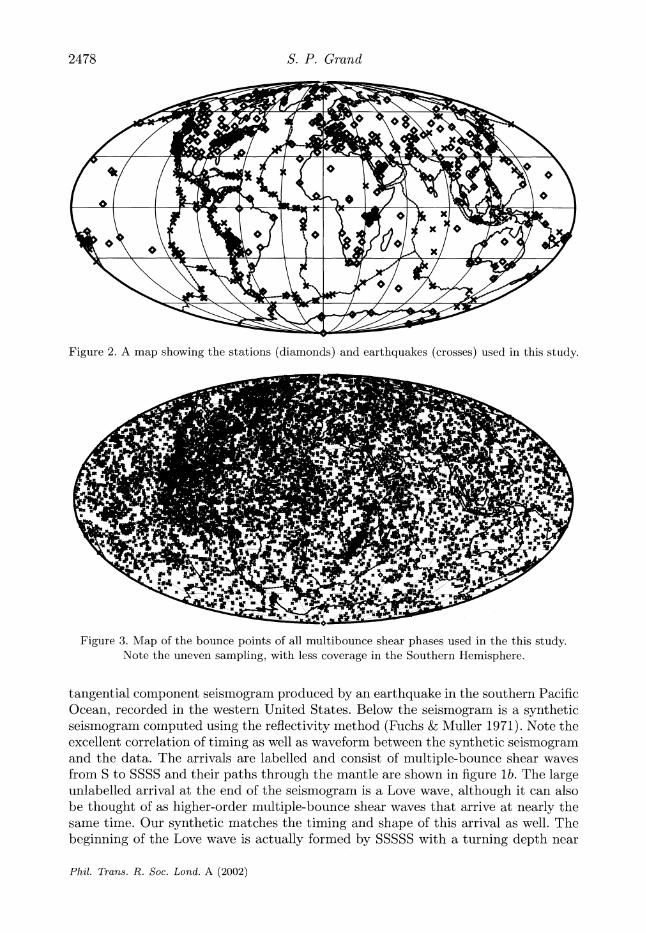
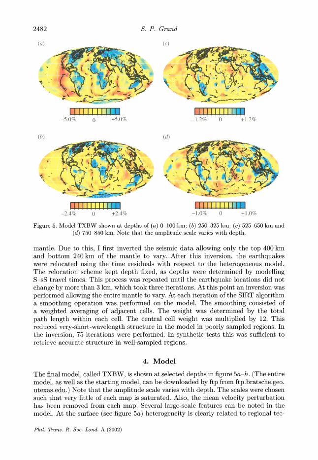
Figure 5. Model TXBW shown at depths of (a) 0-100 km; (b) 250-325 km; (c) 525-650 km and (d) 750-850 km. Note that the amplitude scale varies with depth.

mantle. Due to this, I first inverted the seismic data allowing only the top 400 km and bottom 240 km of the mantle to vary. After this inversion, the earthquakes were relocated using the time residuals with respect to the heterogeneous model. The relocation scheme kept depth fixed, as depths were determined by modelling S-sS travel times. This process was repeated until the earthquake locations did not change by more than 3 km, which took three iterations. At this point an inversion was performed allowing the entire mantle to vary. At each iteration of the SIRT algorithm a smoothing operation was performed on the model. The smoothing consisted of a weighted averaging of adjacent cells. The weight was determined by the total path length within each cell. The central cell weight was multiplied by 12. This reduced very-short-wavelength structure in the model in poorly sampled regions. In the inversion, 75 iterations were performed. In synthetic tests this was sufficient to retrieve accurate structure in well-sampled regions.

4. Model

The final model, called TXBW, is shown at selected depths in figure 5a-h. (The entire model, as well as the starting model, can be downloaded by ftp from ftp.bratsche.geo. utexas.edu.) Note that the amplitude scale varies with depth. The scales were chosen such that very little of each map is saturated. Also, the mean velocity perturbation has been removed from each map. Several large-scale features can be noted in the model. At the surface (see figure 5a) heterogeneity is clearly related to regional tec-


2482


(e)

EmII I II 1.0% 0 +1.0%

(f,

ir'I Iiim -1.0% 0 +1.0%

(g)

I I I I

(h)

IT Ii

-2.0% 0 +2.0%

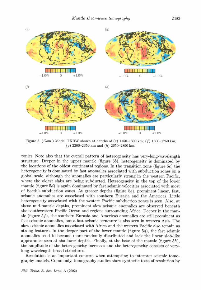
Figure 5. (Cont.) Model TXBW shown at depths of (e) 1150-1300 km; (f) 1600-1750 km; (g) 2200-2350 km and (h) 2650-2890 km.

tonics. Note also that the overall pattern of heterogeneity has very-long-wavelength structure. Deeper in the upper mantle (figure 5b), heterogeneity is dominated by the locations of the oldest continental regions. In the transition zone (figure 5c) the heterogeneity is dominated by fast anomalies associated with subduction zones on a global scale, although the anomalies are particularly strong in the western Pacific, where the oldest slabs are being subducted. Heterogeneity in the top of the lower mantle (figure 5d) is again dominated by fast seismic velocities associated with most of Earth's subduction zones. At greater depths (figure 5e), prominent linear, fast, seismic anomalies are associated with southern Eurasia and the Americas. Little heterogeneity associated with the western Pacific subduction zones is seen. Also, at these mid-mantle depths, prominent slow seismic anomalies are observed beneath the southwestern Pacific Ocean and regions surrounding Africa. Deeper in the mantle (figure 5f), the southern Eurasia and Americas anomalies are still prominent as fast seismic anomalies, but a fast seismic structure is also seen in western Asia. The slow seismic anomalies associated with Africa and the western Pacific also remain as strong features. In the deeper part of the lower mantle (figure 5g), the fast seismic anomalies tend to become more randomly distributed and lack the linear slab-like appearance seen at shallower depths. Finally, at the base of the mantle (figure 5h), the amplitude of the heterogeneity increases and the heterogeneity consists of very- long-wavelength broad structures.

Resolution is an important concern when attempting to interpret seismic tomography models. Commonly, tomography studies show synthetic tests of resolution by


2483

S. P. Grand

creating an artificial-input structural model, computing the predicted seismic anomalies produced by the structure for a given dataset and then inverting the synthetic data to compare with the starting model. An alternative way to assess resolution is to invert subsets of data and compare results. As mentioned in the introduction, several groups of researchers have produced global shear-wave models of the mantle, using different datasets and methods. In figure 6 we compare five global models, includ- ing model TXBW, which have been produced by different groups. The models were taken from the Reference Earth Model (REM) Web site at http://mahi.ucsd.edu/ Gabi/rem.html. The Scripps model is discussed in Masters et al. (2000), the Harvard model is from Gu et al. (2001), the Berkeley model is from Megnin & Romanowicz (2000) and the Caltech model is from Ritsema et al. (1999). Comparisons of the models are shown at two depths. Other depths can be compared by checking the REM Web site.

Many differences are apparent between the models shown in figure 6, particularly with respect to slow regions. The difference between model TXBW and the other models is most pronounced in the transition zone. It is likely that some heterogeneity in the transition zone has been mapped into the shallower mantle in model TXBW. Also, model TXBW allows a shorter wavelength structure than the other models. When the smoothing is made stronger in model TXBW, the structure near 600 km in depth is more similar to the other models, although the variance reduction is smaller. It should be noted that model TXBW at 600 km depth is more similar to the high-resolution P-wave models derived using ISC data (Fukao et al. 2001). In any case, the prominent high-velocity anomalies at 600 km depth are mostly associated with western Pacific subduction zones and subduction beneath South America. Except for the Harvard model, most of these fast subduction-zone anomalies are limited to widths of the order of 1000 km. The comparison at 1200 km in depth also shows many differences among the models. All the models, however, show two linear fast anomalies, one beneath southern Eurasia and the other beneath the Americas, although the details of the features vary between models. Another fast anomaly is seen beneath the Tonga subduction zone in all models. The large linear features also compare well with P-wave tomography models (Grand et al. 1997). These three fast structures are the only fast anomalies common to all the models. It is thus likely that these structures are real features within the Earth. Note that there is very little fast mantle seen beneath most of the western Pacific and eastern Asian subduction zones in any of the models at 1200 km depth.

5. Discussion

Although global tomographic images still have large uncertainties, some robust large- scale patterns have emerged that I feel place constraints on flow in the mantle. Here I will discuss the fast seismic anomalies seen in model TXBW and relate the images to downward flow in the mantle. I will focus on aspects of the model that are robust in the sense that similar features are seen in most other tomography models, although details may vary. In many studies such a discussion is given with cross-sections through seismic models. Cross-sections, however, can be chosen to show just about whatever the author wants to show depending on how they are chosen. Here, I prefer to concentrate on the overall patterns seen in the seismic model and this is best done with reference to the constant depth maps shown in figure 5a-h.


2484


Structure at shallow depths is relatively long wavelength and dominated by tec- tonic province (figure 5a, b). At depths above 400 km, subducting slabs are not apparent in global shear-wave images, probably due to their being smaller than the resolv- ing power in the images. Deeper than 400 km, the fast anomalies are likely to be related to downwellings in the convecting mantle. Just above the 660 km discontinuity, strong, fast seismic anomalies are seen, associated with almost every subduction zone (figures 5c and 6). The exceptions are where relatively young lithosphere is being subducted, such as the Juan de Fuca plate and the northern Cocos plate. Given that slabs are not well imaged in any of the global-shear models at shallower depths, for example at 300 km depth in figure 5b, it is likely that the images near 600 km in depth indicate that subducting slabs meet significant resistance to flow into the deeper mantle and therefore pile up above 660 km depth. This is consistent with several high-resolution studies of slab structure that show some slabs flattening above 660 km in depth (see, for example, Zhou & Clayton 1990; van der Hilst & Seno 1993; van der Hilst 1995; Ding & Grand 1994; Fukao et al. 2001). A second observation is that the fast seismic anomalies near 600 km in depth are not very long wavelength, as observed, for example, at the surface (figure 5a). In my model, the transition-zone anomalies are mostly linear in shape and rarely wider than 1000 km. In other studies (figure 6), the transition-zone anomalies are broader but rarely beyond 1500 km in width, except for the Harvard model. It should be noted that tomography results will tend to broaden anomalies relative to their actual dimensions. Fukao et al. (2001) compare in detail high-resolution images derived from P-waves with two of the shear models shown in figure 6. They find the shear models do indeed overestimate the width of the transition-zone anomalies. Engebretson et al. (1992) estimate the total convergence perpendicular to trenches for various subduction zones. They find for sites ranging from the Japan trench to the Himalayan suture that 3000-5000 km of slab has subducted during the past 50 Myr. The seismic models do not show fast anomalies in the transition zone with nearly the dimensions to account for the vol- ume of slab subducted during the past 50 Myr. Unless subducted slabs can reach thermal equilibrium with the surrounding upper mantle on time-scales significantly less than 50 Myr, the tomography models indicate that, although slabs encounter resistance to flow near 660 km in depth, they do penetrate deeper into the mantle at some point in time.

Figure 5d shows fast seismic anomalies associated with all subduction zones to depths exceeding 850 km. These anomalies are largely linear on a large scale and are most likely to be subducted lithosphere. By 1200 km in depth, however, fast seismic anomalies are only associated with North America and southern Eurasia (figure 5e). As seen in figure 6, the two large fast structures are seen in most global tomography shear-wave models. van der Hilst et al. (1997) have seen similar structures in P- wave tomographic models and have named the two structures the Farallon anomaly and the Tethyan anomaly, respectively. These linear fast anomalies have naturally been interpreted as subducted lithosphere descending into the deep mantle (Grand 1994; van der Hilst et al. 1997; Van der Voo et al. 1999). However, it is interesting to note that there is little indication of any fast seismic anomalies associated with the western Pacific or eastern Asian subduction zones at these depths. Bunge et al. (1998) show that if slabs sink uniformly through the lower mantle such that the Farallon and Tethyan anomalies are ancient subducted slabs, then one should observe similar linear features beneath eastern Asia. In other words, there has been


2485

S. P. Grand

(>(cc) w

?. ''/' ?i....

iiiiiii E11 1111 i ' !tl I I I i I J I [ It[ ~ I 1 I I I I I I I i -1.2% 0 +1.2% -1.0% 0 +1.0%

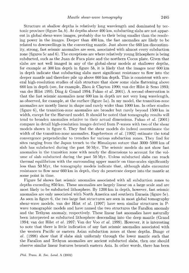
Figure 6. A comparison of five global shear-wave models of Earth's mantle. The Berkeley model (a) is from Megnin & Romanowicz (2000), the Caltech model (b) from Ritsema et al. (1999), the Harvard model (c) from Gu et al. (2001), the Scripps model (d) from Masters et al. (2000) and the Texas model (e) is presented in this paper. Depths are: left, 600 km; right, 1200 km.

just as much, if not more, convergence in subduction zones over the past 100 Myr in the western Pacific compared with southern Eurasia and the Americas. The lack of continuity of fast anomalies into the deep mantle beneath western Pacific subduction zones has led Fukao et al. (2001) to propose that slabs remain stagnant in the mantle above ca. 1000 km in depth. Indeed, Niu & Kawakatsu (1997) find a variable- depth seismic discontinuity near 1000 km in depth associated with western Pacific subduction zones. Also, Wen & Anderson (1998) find that the geoid and topography of Earth are best fitted with a barrier to flow near 1000 km in depth. A problem with a barrier near 1000 km depth is that the Tethyan and Farallon slabs seem to penetrate much deeper than 1000 km with little distortion. Also, Niu & Kawakatsu (1997) find significant variability in the depth of the mid-mantle discontinuity unrelated to subduction history.

An alternative explanation for the difference in apparent lower-mantle flow for different subduction regions could involve time dependence of flow across the 660 km


2486


(d)

(e)

t I I I I I 11111 II I 1111111 I 11 -1.2% 0 +1.2% -1.0% 0 +1.0%

Figure 6. (Cont.)

discontinuity. Solheim & Peltier (1994), Tackley (1995) and others have shown that if the 660 km discontinuity represents an endothermic phase change, it may strongly impede flow and in some cases may result in episodic flow through the boundary. As the tomography results are only a snapshot in time of mantle structure, it may be that the apparent pile up of slab near 1000 km depth is just the result of material that had been piled up near 660 km in depth in the past but has recently begun sink-

ing into the lower mantle. It has also been proposed that mantle viscosity increases near 660 km and again near 1000 km depth (Mitrovica & Forte 1997). A viscosity increase will cause some horizontal flow at the depth at which the subducting material encounters the higher viscosity region (Gurnis & Hager 1988). Many of the fast anomalies seen near 850 km depth seem to be rather broad as well as offset from the deepest seismicity. This has led Fukao et al. (2001) to conclude that there is

stagnation of slab above 1000 km in depth. With horizontal spreading of slabs at 660 km depth and time-dependent sinking, it is possible that the images at greater depths do not represent resistance to flow near 1000 km in depth, but rather just indicate a complex prior history at shallower depths. At greater depths in the mantle near 1600 km (figure 5f), eastern Asian fast anomalies are again apparent in the tomography models. The Farallon and Tethyan anomalies are also visible at these depths. The observation of deeper fast anomalies associated with the Pacific subduction zones is most consistent with a time-dependent flow across some shallower boundary but with eventual sinking of most slabs to much deeper depths.

The seismic fast anomalies seen in the lower mantle have also been proposed to be due to conductive cooling of the lower mantle by slabs in the upper mantle causing downwellings in the lower mantle. The fact that the western Pacific regions show a hiatus in slab fast anomalies with depth seems to argue against this. Subduction beneath the northwest Pacific has been continuous for over 100 Myr (Engebretson et al. 1992; Lithgow-Bertelloni et al. 1993). This would imply a continuous process of


2487

conductive cooling of the lower mantle in this region that should produce a continuous

downwelling in the lower mantle in this region, as is seen with the Tethyan and Farallon anomalies.

The deeper part of the lower mantle (figure 5g) shows no clear linear, fast seismic

anomalies, as are seen in the mid-mantle. A loss of clear slab-like anomalies is also seen in the P-wave-tomography model of van der Hilst et al. (1997). This led van der Hilst & Karason (1999) and Kellogg et al. (1999) to propose a deep, chemically distinct, lower mantle, through which slabs do not fully penetrate. Although the linear features are not seen in the deeper lower mantle, the regions of fast velocity are found in regions associated with the shallower fast linear anomalies. Furthermore, at the base of the mantle (figure 5h), strong, long-wavelength, fast anomalies are found, associated with all regions of ancient subduction. This feature is very robust and in fact was seen in the earliest tomographic models (Dziewonski 1984; Dziewonski & Woodhouse 1987). Although there are no clear linear fast features that are continuous throughout the lower mantle to the core-mantle boundary, I think there are several reasons that make it likely that the faster regions in the deepest mantle are indeed slab-derived material. First, only at the top of the mantle and the base of the mantle does one see very-long-wavelength structures, which are indicative of a thermal boundary layer. Second, the boundaries between broad, slow and broad, fast

regions in the deepest mantle seem to be very abrupt. In fact, Wen et al. (2001) and Wen (2001) have found that the boundaries between the fast and slow regions in the

deepest mantle are very sharp. They conclude that the slow regions in the deepest mantle are likely to be chemically distinct from the faster regions. If this is true, and slabs are not reaching the core-mantle boundary due to a shallower chemical

boundary, then three chemically distinct regions of the mantle are required. This seems unlikely. The break-up of the linear-slab anomalies at depths near to 2000 km, as well as the large, slow, seismic anomalies seen at these depths, may be due to an increase in viscosity in the deeper mantle, as proposed by Forte & Mitrovica (2001).

6. Conclusion

In this paper I have presented a new global model of mantle shear velocities. Com-

parison of the model with other global shear-wave models shows good agreement with respect to large-scale, fast, seismic anomalies although there are many clear contradictions among the models. With respect to downward flow in the mantle, tomography models show that simple continuous flow of mantle from shallow depths to the base of the mantle is highly unlikely. Changes in the pattern of heterogeneity are visible in the lower mantle at depths near 1000 km and 2000 km. Both depths have been proposed as depths where a chemical or other type of boundary exists

inhibiting downward flow. An alternative explanation for some of the complexity seen in the patterns of fast seismic anomalies is that there is a time dependence of flow through the 660 km discontinuity, resulting in an irregular distribution of slab in the lower mantle. The deeper mantle exhibits longer-wavelength structures that

may be due to an increase in viscosity in the deepest mantle.

I thank the Northern California Earthquake Data Center and Berkeley Seismological Laboratory, as well as the Canadian National Seismological Data Center, for providing seismic data. Also

greatly appreciated are data from the IRIS GSN network and the French Geoscope network. I

also thank Gabi Laske for creating the REM Web page and for helping with downloading other


2488 S. P. Grand


tomographic models, Michael Bostock for sending data, Ed Garnero for teaching me SAC and Mrinal Sen for use of his reflectivity code. Whitney Goodrich helped to prepare some of the

figures. This research was supported by NSF grants EAR-9725335 and EAR-0073643.

References

Bijwaard, H., Spakman, W. & Engdahl, E. R. 1998 Closing the gap between regional and global travel time tomography. J. Geophys. Res. 103, 30055-30078.

Bunge, H. P., Richards, M. A., Lithgow-Bertelloni, C., Baumgardner, J. R., Grand, S. P. & Romanowicz, B. A. 1998 Time scales and heterogeneous structure in geodynamic Earth models. Science 280, 91-95.

Ding, X. Y. & Grand, S. P. 1994 Seismic structure of the deep Kurile subduction zone. J. Geophys. Res. 99, 23 767-23 786.

Dziewonski, A. M. 1984 Mapping the lower mantle: determination of lateral heterogeneity in P velocity up to degree and order 6. J. Geophys. Res. 89, 5929-5952.

Dziewonski, A. M. & Anderson, D. L. 1981 Preliminary reference Earth model. Phys. Earth Planet. Inter. 25, 297-356.

Dziewonski, A. M. & Gilbert, F. 1976 The effect of small, aspherical perturbations on travel times and a re-examination of the corrections for ellipticity. Geophys. J. R. Astr. Soc. 44, 7-17.

Dziewonski, A. M. & Woodhouse, J. H. 1987 Global images of the Earth's interior. Science 236, 37-48.

Engebretson, D. C., Kelley, K. P., Cashman, H. J. & Richards, M. A. 1992 180 million years of subduction. GSA Today 2, 93-100.

Forte, A. M. & Mitrovica, J. X. 2001 Deep mantle high viscosity flow and thermochemical structure inferred from seismic and geodynamic data. Nature 410, 1049-1056.

Fuchs, K. & Muller, G. 1971 Computation of synthetic seismograms with the reflectivity method and comparison with observations. Geophys. J. R. Astr. Soc. 23, 417-433.

Fukao, Y., Widiyantoro, S. & Obayashi, M. 2001 Stagnant slabs in the upper and lower mantle transition zone. Rev. Geophys. 39, 291-323.

Grand, S. P. 1994 Mantle shear structure beneath the Americas and surrounding oceans. J. Geophys. Res. 99, 11591-11621.

Grand, S. P. & Helmberger, D. V. 1984 Upper mantle shear structure of North America. Geophys. J. R. Astr. Soc. 76, 399-438.

Grand, S. P., van der Hilst, R. D. & Widiyantoro, S. 1997 Global seismic tomography: a snapshot of convection in the Earth. GSA Today 7(4), 1-7.

Gu, Y. J., Dziewonski, A. M., Su, W. & Ekstrom, G. 2001 Models of the mantle shear velocity and discontinuities in the pattern of lateral heterogeneity. J. Geophys. Res. 106, 11 169-11 199.

Gurnis, M. & Hager, B. H. 1988 Controls on the structure of subducted slabs. Nature 335, 317-321.

Hager, B. H. & Clayton, R. W. 1989 Constraints on the structure of mantle convection. In Mantle convection: plate tectonics and global dynamics (ed. W. R. Peltier). New York: Gordon & Breach.

Hamilton, W. B. 2002 The closed upper-mantle circulation of plate tectonics. In Plate boundary zones (ed. S. Stein & J. Freymueller). AGU Geophysical Monograph. (In the press.)

Helmberger, D. V. & Engen, G. R. 1974 Upper mantle shear structure. J. Geophys. Res. 79, 4017-4028.

Karason, H. & van der Hilst, R. D. 2000 Constraints on mantle convection from seismic tomography. In The history and dynamics of global plate motion (ed. M. R. Richrds, R. Gordon & R. D. van der Hilst). AGU Geophysical Monograph vol. 212, pp. 277-288.


2489

S. P. Grand

Kellogg, L. H., Hager, B. H. & van der Hilst, R. D. 1999 Compositional stratification in the deep mantle. Science 283, 1181-1184.

Lithgow-Bertelloni, C., Richards, M. A., Ricard, Y., O'Connell, R. J. & Engebretson, D. C. 1993 Toroidal-poloidal partitioning of plate motions since 120 Ma. Geophys. Res. Lett. 20, 375-378.

Masters, T. G., Laske, G., Bolton, H. & Dziewonski, A. 2000 The relative behavior of shear velocity, bulk sound speed and compressional velocity in the mantle: implications for chemical thermal structure, in Earth's deeep interior. Mineral physics and tomography from the atomic to the global scale (ed. S. Karato et al.). AGU Geophysical Monograph, vol. 117, pp. 63-87. Washington, DC.

Megnin, C. & Romanowicz, B. 2000 The three-dimensional shear velocity structure of the mantle from the inversion of body, surface and higher-mode waveforms. Geophys. J. Int. 143, 709- 728.

Mitrovica, J. X. & Forte, A. M. 1997 Radial profile of mantle viscosity: results from the joint inversion of convection and postglacial rebound observables. J. Geophys. Res. 102, 2751-2770.

Mooney, W. D., Laske, G. & Masters, T. G. 1998 CRUST 5.1: a global crustal model at 5 x 5 degrees. J. Geophys. Res. 103, 727-747.

Niu, F. & Kawakatsu, H. 1997 Depth variation of the midmantle seismic discontinuity. Geophys. Res. Lett. 24, 429-432.

Obayashi, M., Sakurai, T. & Fukao, Y. 1997 Comparison of recent tomographic models. In Proc. Int. Symp. on New Images of the Earth's Interior Through Long Term Ocean-Floor Observa- tions, Earthquake Research Institute, University of Tokyo, Tokyo, Japan (ed. K. Suyehiro).

Richards, M. A. & Engebretson, D. C. 1992 Large-scale mantle convection and the history of subduction. Nature 355, 437-440.

Ritsema, J., van Heijst, H. J. & Woodhouse, J. H. 1999 Complex shear wave velocity structure imaged beneath Africa and Iceland. Science 286, 1925-1928.

Robertson, G. S. & Woodhouse, J. H. 1996 Ratio of relative S to P velocity heterogeneity in the lower mantle. J. Geophys. Res. 101, 20041-20052.

Solheim, L. P. & Peltier, W. R. 1994 Avalanche effects in phase transition modulated thermal convection: a model of Earth's mantle. J. Geophys. Res. 99, 6997-7018.

Spakman, W., van der Lee, S. & van der Hilst, R. D. 1993 Travel-time tomography of the European-Mediterranean mantle down to 1400 km. Phys. Earth Planet. Inter. 79, 3-74.

Tackley, P. J. 1995 On the penetration of an endothermic phase transition by upwellings and downwellings. J. Geophys. Res. 100, 15477-15488.

van der Hilst, R. D. 1995 Complex morhpology of subducted lithosphere in the mantle beneath the Tonga trench. Nature 374, 154-157.

van der Hilst, R. D. & Karason, H. 1999 Compositional heterogeneity in the bottom 1000 kilo- meters of Earth's mantle: toward a hybrid convection model. Science 283, 1885-1888.

van der Hilst, R. D. & Seno, T. 1993 Effects of relative plate motion on the deep structure and penetration depth of slabs below the Izu-Bonin and Mariana island arcs. Earth Planet. Sci. Lett. 120, 375-407.

van der Hilst, R. D., Widiyantoro, S. & Engdahl, E. R. 1997 Evidence for deep mantle circulation from global tomography. Nature 386, 578-584.

van der Voo, R., Spakman, W. & Bijwaard, H. 1999 Tethyan subducted slabs under India. Earth Planet. Sci. Lett. 171, 7-20.

Wen, L. 2001 Seismic evidence for a rapidly-varying compositional anomaly at the base of the Earth's mantle beneath the Indian Ocean. Earth Planet. Sci. Lett. 194, 83-95.

Wen, L. & Anderson, D. L. 1998 Layered mantle convection: a model for geoid and topography. Earth Planet. Sci. Lett. 146, 367-377.

Wen, L., Silver, P., James, D. & Kuehnel, R. 2001 Seismic evidence for a thermo-chemical boundary layer at the base of Earth's mantle. Earth Planet. Sci. Lett. 189, 141-153.


2490


Widiyantoro, S. & van der Hilst, R. 1996 Structure and evolution of lithospheric slab beneath the Sunda Arc, Indonesia. Science 271, 1566-1570.

Widiyantoro, S., Kennett, B. L. N. & van der Hilst, R. D. 1998 Extending shear-wave tomography for the lower mantle using S and SKS arrival-time data. Earth Planets Space 50, 999-1012.

Zhao, D. 2001 Seismic structure and origin of hotspots and mantle plumes. Earth Planet. Sci. Lett. 192, 251-265.

Zhou, H. & Clayton, R. W. 1990 P and S wave travel-time inversions for subducting slab under the island arcs of the northwest Pacific. Geophys. Res. 95, 6829-6851.


2491

Documents

Mantle Shear-Wave Tomography and the Fate of …rcoe/eart206/Grand_S-waveTomog_PhilTrans...Mantle shear-wave tomography to 200 km. Our approach is to examine all tangential-component