Embed Size (px)
Citation preview

SUSTAINABLE FISHERIES MANAGEMENT PROJECT (SFMP)
Manual for GIS Training of Central
Regional TCPD Officers
2017

i
This publication is available electronically in the following locations:
The Coastal Resources Center
http://www.crc.uri.edu/projects_page/ghanasfmp/
Ghanalinks.org
https://ghanalinks.org/elibrary search term: SFMP
USAID Development Clearing House
https://dec.usaid.gov/dec/content/search.aspx search term: Ghana SFMP
For more information on the Ghana Sustainable Fisheries Management Project, contact:
USAID/Ghana Sustainable Fisheries Management Project
Coastal Resources Center
Graduate School of Oceanography
University of Rhode Island
220 South Ferry Rd.
Narragansett, RI 02882 USA
Tel: 401-874-6224 Fax: 401-874-6920 Email: [email protected]
Citation: Owusu Donkor, P., Mensah, J. C, Adams, O. and Mohammed, M. (2017).
Manual for GIS Training of Central Regional TCPD Officers. The
USAID/Ghana Sustainable Fisheries Management Project (SFMP). Narragansett
, RI: Coastal Resources Center, Graduate School of Oceanography, University of
Rhode Island and Spatial Solutions, #3 Third Nautical Close, Nungua, Accra. 31
pp.
Authority/Disclaimer:
Prepared for USAID/Ghana under Cooperative Agreement (AID-641-A-15-00001) awarded
on October 22, 2014 to the University of Rhode Island and entitled; the USAID/Ghana
Sustainable Fisheries Management Project (SFMP).
This document is made possible by the support of the American People through the United
States Agency for International Development (USAID). The views expressed and opinions
contained in this report are those of the SFMP team and are not intended as statements of
policy of either USAID or the cooperating organizations. As such, the contents of this report
are the sole responsibility of the SFMP Project team and do not necessarily reflect the views
of USAID or the United States Government.
Cover photo: Group photograph of some of the beneficiaries of the training. Credit: Spatial
Solutions.

ii
USAID/Ghana Sustainable Fisheries Management Project (SFMP) 10 Obodai St., Mempeasem, East Legon, Accra, Ghana
Telephone: +233 0302 542497 Fax: +233 0302 542498
Maurice Knight Chief of Party [email protected]
Kofi Agbogah Senior Fisheries Advisor [email protected]
Nii Odenkey Abbey Communications Officer [email protected]
Bakari Nyari Monitoring and Evaluation Specialist [email protected]
Brian Crawford Project Manager, CRC [email protected]
Ellis Ekekpi USAID AOR (acting) [email protected]
Kofi.Agbogah
Stephen Kankam
Hen Mpoano
38 J. Cross Cole St. Windy Ridge
Takoradi, Ghana
233 312 020 701
Andre de Jager
SNV Netherlands Development Organisation
#161, 10 Maseru Road,
E. Legon, Accra, Ghana
233 30 701 2440
Donkris Mevuta
Kyei Yamoah
Friends of the Nation
Parks and Gardens
Adiembra-Sekondi, Ghana
233 312 046 180
Resonance Global
(formerly SSG Advisors)
182 Main Street
Burlington, VT 05401
+1 (802) 735-1162
Thomas Buck
Victoria C. Koomson
CEWEFIA
B342 Bronyibima Estate
Elmina, Ghana
233 024 427 8377
Lydia Sasu
DAA
Darkuman Junction, Kaneshie Odokor
Highway
Accra, Ghana
233 302 315894
For additional information on partner activities:
CRC/URI: http://www.crc.uri.edu
CEWEFIA: http://cewefia.weebly.com/
DAA: http://womenthrive.org/development-action-association-daa
Friends of the Nation: http://www.fonghana.org
Hen Mpoano: http://www.henmpoano.org
SNV: http://www.snvworld.org/en/countries/ghana
Resonance Global: https://resonanceglobal.com/

ii
ACRONYMS
CRS Coordinate Reference System
ESPG European Petroleum Search Group
ESRI Environmental Sciences Research Institute
GDAL Geospatial Data Abstraction Library
GIS Geographic Information System
GPS Global Positioning System
GUI Graphical User Interface
ICFG Integrated Coastal and Fisheries Governance
IGNF Institut Geographique National de France
OGR OpenGIS Simple Features Reference Implementation
QGIS Quantum GIS
SFMP Sustainable Fisheries Management Program
TCPD Town and Country Planning Department
USAID United States Agency for International Development

iii
TABLE OF CONTENTS
ACRONYMS ............................................................................................................................. ii
TABLE OF CONTENTS ......................................................................................................... iii
LIST OF FIGURES ................................................................................................................. iii
INTRODUCTION ..................................................................................................................... 1
Objectives .............................................................................................................................. 1
BASIC GIS AND FILE MANAGEMENT ............................................................................... 1
Organizing the Working Directory ........................................................................................ 1
QGIS interface ....................................................................................................................... 2
Adding a Vector Layer........................................................................................................... 3
Loading a Shapefile ........................................................................................................... 4
Adding Raster data in QGIS .................................................................................................. 5
Symbology ............................................................................................................................. 6
Changing Colors ................................................................................................................ 6
Changing Symbol Structure ............................................................................................... 7
DATA ACQUISITION (PRIMARY AND SECONDARY SOURCES) .................................. 9
Using GPS data ...................................................................................................................... 9
Digitizing ............................................................................................................................. 10
Creating an empty shapefile ............................................................................................. 10
Adding data to your shapefile .......................................................................................... 12
DATA FORMATS AND DATA INTEROPERABILITY ...................................................... 15
Supported Data Formats ...................................................................................................... 15
Vector Data Formats ........................................................................................................ 15
Raster Data formats.......................................................................................................... 15
Coordinate Systems and data Projections ........................................................................ 15
PRACTICAL EXERCISE ....................................................................................................... 16
Capturing data from Google Earth into QGIS for georeferencing ...................................... 16
LIST OF FIGURES
Figure 1 Create file folder .......................................................................................................... 2 Figure 2 The QGIS Graphical User Interface ............................................................................ 3 Figure 3 Add Vector Layer menu option ................................................................................... 4 Figure 4 Selecting a shapefile from the list and clicking ‘Open’ loads it into QGIS ................ 5
Figure 5 Open a GDAL Supported Raster Data Source dialog. ................................................ 6 Figure 6 In the ‘Properties’ window, select the ‘Style’ tab at the extreme left ........................ 7 Figure 7 Open the‘Layer Properties’ window for the layer ....................................................... 8
Figure 8 To load a GPX file, you first need to load the plugin.................................................. 9 Figure 9 Browse to the folder containing the GPX file ........................................................... 10 Figure 10 New shapefile Layer ................................................................................................ 11 Figure 11 Give the shapefile a short and meaningful name ..................................................... 12

iv
Figure 12 After you click on the map, a window will appear and you can enter all of
the attribute data for that point ................................................................................................. 13 Figure 13 The line stretches like an elastic band to follow the mouse cursor around as you
move it. .................................................................................................................................... 13 Figure 14 Capturing data from Google Earth into QGIS for georeferencing .......................... 16 Figure 15 Search for Elmina .................................................................................................... 17
Figure 16 Generate control points ............................................................................................ 18 Figure 17 Control points .......................................................................................................... 19 Figure 18 Save the control points and image ........................................................................... 20 Figure 19. Load the Control Points saved from Google Earth ................................................ 21 Figure 20 Adding vector .......................................................................................................... 21
Figure 21 Vector data displayed .............................................................................................. 22 Figure 22 Load the image saved (ElminaJpg) into Georeferencer .......................................... 22
Figure 23 Load the image by selecting the Raster and locating the image Elmina ................. 23 Figure 24 Start Georeferencing by adding control points ........................................................ 23 Figure 25 Select the corresponding point (c3) in the QGIS Data view ................................... 24 Figure 26 Click on Play or Run for georeferencing to be effected .......................................... 24 Figure 27 Drag the vector data Elmina on top of Elmina_georef ............................................ 25

1
INTRODUCTION
The USAID-Ghana Sustainable Fisheries Management Project (SFMP) is committed to the
capacity building of Town and Country Planning Department. The project recognizes the
important role the department plays in the planning of the limited coastal land and beach
fronts in the face of rapid coastal erosion and the influx of infrastructure to accommodate the
burgeoning population in coastal communities. The Sustainable Fisheries Management
Project is working to build the capacity of the region’s Town and Country Planning
Department (TCPD) through state-of-the-art facilities and regular trainings aimed at
encouraging coastal resource management in physical planning.
Objectives
The GIS training is one of the activities aimed at activating the Central region GIS Data Hub
to function as the model training center, not only for TCPD staff, but other sister land
agencies and departments. The specific objectives for the training were:
To activate the GIS Data Hub as the data clearinghouse and training center for the region.
To introduce the use of Quantum GIS, GPS and Google earth for basic data collection and
mapping purposes.
This document is the training manual used
BASIC GIS AND FILE MANAGEMENT
Organizing the Working Directory
You can easily manage your files and folders using File/Windows Explorer on a Windows
computer.
The File/Windows Explorer allows you to open, access, and rearrange your files and folders
in Desktop view. It also allows you to create directories (folders) and sub directories for your
project
1. Click the folder icon on the taskbar in Desktop view to open File/Windows
Explorer.
2. Browse to the disc you want to organize your project in.
3. Click the ‘New Folder’ buttons and rename the folder.
2
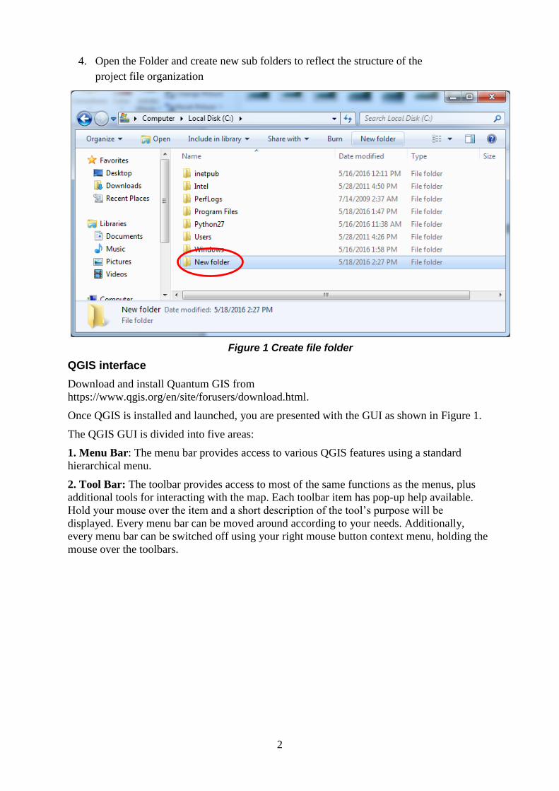
4. Open the Folder and create new sub folders to reflect the structure of the
project file organization
QGIS interface
Download and install Quantum GIS from
https://www.qgis.org/en/site/forusers/download.html.
Once QGIS is installed and launched, you are presented with the GUI as shown in Figure 1.
The QGIS GUI is divided into five areas:
1. Menu Bar: The menu bar provides access to various QGIS features using a standard
hierarchical menu.
2. Tool Bar: The toolbar provides access to most of the same functions as the menus, plus
additional tools for interacting with the map. Each toolbar item has pop-up help available.
Hold your mouse over the item and a short description of the tool’s purpose will be
displayed. Every menu bar can be moved around according to your needs. Additionally,
every menu bar can be switched off using your right mouse button context menu, holding the
mouse over the toolbars.
Figure 1 Create file folder

3
Tip: Restoring toolbars If you have accidentally hidden all your toolbars, you can get them
back by choosing menu option Settings → Toolbars →.
3. Map Legend: The map legend area lists all the layers in the project. The checkbox in each
legend entry can be used to show or hide the layer. A layer can be selected and dragged up or
down in the legend to change the Z-ordering. Z-ordering means that layers listed nearer the
top of the legend are drawn over layers listed lower down in the legend.
4. Map View: Maps are displayed in this area. The map displayed in this window will
depend on the vector and raster layers you have chosen to load. The map view can be panned,
shifting the focus of the map display to another region, and it can be zoomed in and out.
Various other operations can be performed on the map as described in the toolbar description
above. The map view and the legend are tightly bound to each other — the maps in view
reflect changes you make in the legend area.
5. Status Bar: The status bar shows you your current position in map coordinates (e.g.,
meters or decimal degrees) as the mouse pointer is moved across the map view. To the left of
the coordinate display in the status bar is a small button that will toggle between showing
coordinate position or the view extents of the map view as you pan and zoom in and out.
Next to the coordinate display you will find the scale display. It shows the scale of the map
view. If you zoom in or out, QGIS shows you the current scale.
Adding a Vector Layer
The standard vector file format used in QGIS is the ESRI shapefile. A shapefile actually
consists of several files. The following three are required:
Figure 2 The QGIS Graphical User Interface

4
.shp file containing the feature geometries
.dbf file containing the attributes in dBase format
.shx index file
Shapefiles also can include a file with a .prj suffix, which contains the projection information.
While it is very useful to have a projection file, it is not mandatory. A shapefile dataset can
contain additional files.
Lo
→ Add Vector Layer menu option. This will bring up a new window
ading a Shapefile
To load a shapefile, click on the Add Vector Layer toolbar button or by select the Layer
Figure 3 Add Vector Layer menu option
From the available options check File.
Click on ‘Browse’. That will bring up a standard open file dialog which allows you to
navigate the file system and load a shapefile or other supported data source.
The selection box Filter allows you to preselect some OGR-supported file formats. More than
one layer can be loaded at the same time by holding down the Ctrl or Shift key and clicking
on multiple items.

5
Figure 4 Selecting a shapefile from the list and clicking ‘Open’ loads it into QGIS
Selecting a shapefile from the list and clicking ‘Open’ loads it into QGIS.
Tip: Layer Colors
When you add a layer to the map, it is assigned a random color. When adding more than one
layer at a time, different colors are assigned to each layer.
Once a shapefile is loaded, you can zoom around it using the map navigation tools. To
change the style of a layer, open the Layer Properties dialog by double clicking on the layer
name or by right-clicking on the name in the legend and choosing Properties from the context
menu (Refer to Symbology for more on styling layers).
Adding Raster data in QGIS
Raster layers are loaded either by clicking on the Add Raster Layer icon or by selecting
the Layer → Add Raster Layer menu option. More than one layer can be loaded at the
same time by holding down the Ctrl or Shift key and clicking on multiple items in the Open a
GDAL Supported Raster Data Source dialog.

6
Figure 5 Open a GDAL Supported Raster Data Source dialog.
Symbology
The symbology of a layer is its visual appearance on the map. The basic strength of GIS over
other ways of representing data with spatial aspects is that with GIS, you have a dynamic
visual representation of the data you’re working with.
Changing Colors
To change a vector layer’s symbology;
Select the menu item ‘Properties’ in the menu that appears. you can also access a layer’s
properties by double-clicking on the layer in the Layers list
In the ‘Properties’ window, select the ‘Style’ tab at the extreme left:

7
Click the color select button next to the ‘color’ label.
A standard color dialog will appear.
Choose a color and click ‘OK’
Click ‘OK’ again in the ‘Layer Properties’ window, and you will see the color change
being applied to the layer.
Changing Symbol Structure
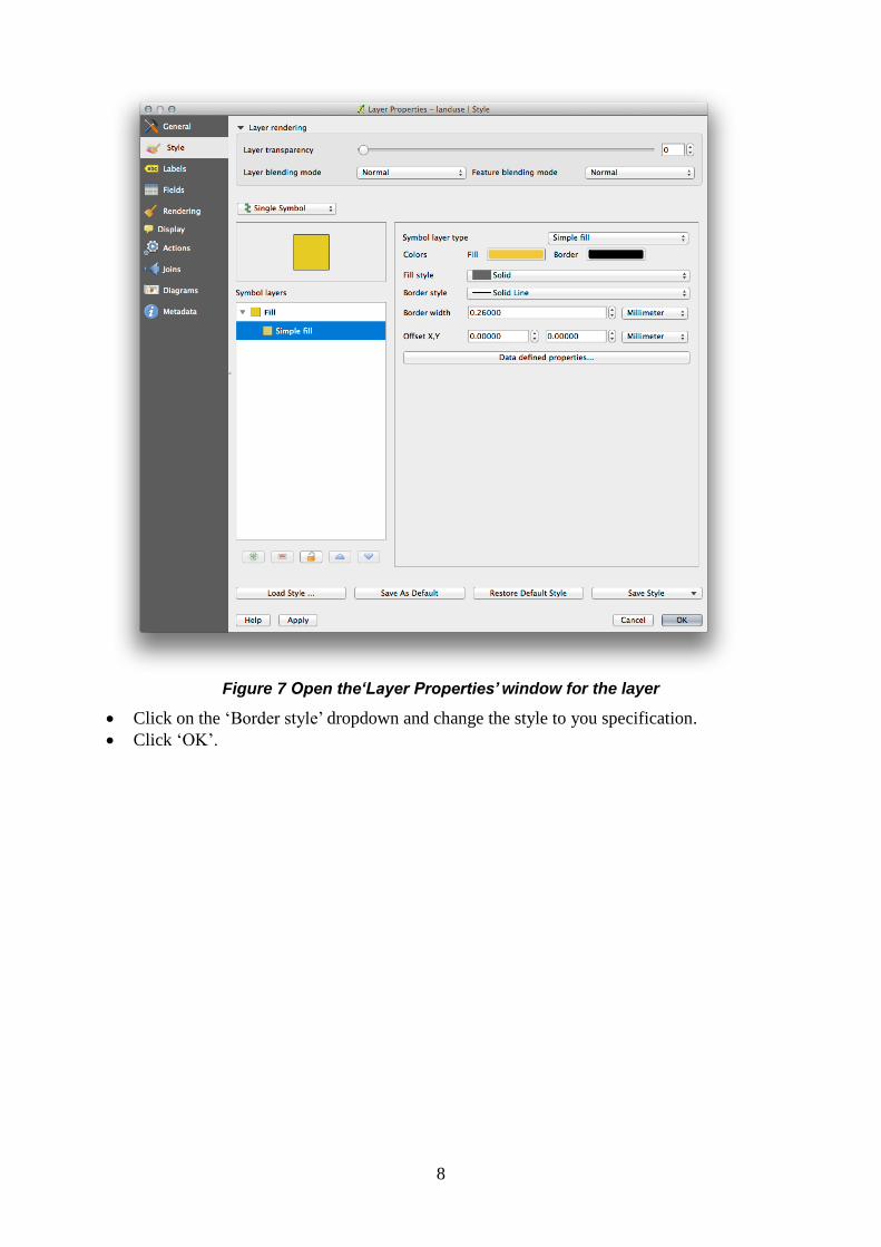
Open the ‘Layer Properties’ window for the layer.
In the ‘Symbol Layer’ panel under the ‘Style’ tab, expand the ‘fill’ dropdown (if
necessary) and select the ‘simple fill’ option:
Figure 6 In the ‘Properties’ window, select the ‘Style’ tab at the extreme left
8
Figure 7 Open the‘Layer Properties’ window for the layer
Click on the ‘Border style’ dropdown and change the style to you specification.
Click ‘OK’.

9
DATA ACQUISITION (PRIMARY AND SECONDARY SOURCES)
One major component of GIS is geospatial data. There are 2 main sources of all geospatial
data- Primary and secondary sources. Primary data are collected on the ground with
surveying instruments or GPS receivers. Another way Planners acquire data is retrieving
needed information from existing data like aerial photos, scanned topographic maps, scanned
sector layouts, etc.
Using GPS data
Loading GPS data from a file
There are dozens of different file formats for storing GPS data. The format that QGIS uses is
called GPX (GPS eXchange format), which is a standard interchange format that can contain
any number of waypoints, routes and tracks in the same file.
To load a GPX file, you first need to load the plugin.
Plugins→ Plugin Manager... opens the Plugin Manager Dialog. Activate the GPS Tools
checkbox. When this plugin is loaded, two buttons with a small handheld GPS device will
show up in the toolbar:
• Create new GPX Layer
• GPS Tools
Figure 8 To load a GPX file, you first need to load the plugin
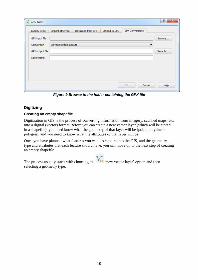
1. Select Vector→GPS→GPS Tools or click the ‘GPS Tools’ icon in the toolbar and
open the ‘Load GPX file’ tab.
2. Browse to the folder containing the GPX file. Select the file and click ‘Open’.
Use the ‘Browse’ button to select the GPX file, and then use the checkboxes to select the
feature types you want to load from that GPX file. Each feature type will be loaded in a
separate layer when you click ‘OK’.
10
Figure 9 Browse to the folder containing the GPX file
Digitizing
Creating an empty shapefile
Digitization in GIS is the process of converting information from imagery, scanned maps, etc.
into a digital (vector) format Before you can create a new vector layer (which will be stored
in a shapefile), you need know what the geometry of that layer will be (point, polyline or
polygon), and you need to know what the attributes of that layer will be.
Once you have planned what features you want to capture into the GIS, and the geometry
type and attributes that each feature should have, you can move on to the next step of creating
an empty shapefile.
The process usually starts with choosing the ‘new vector layer’ option and then
selecting a geometry type.

11
Figure 10 New shapefile Layer
Next you will add fields to the attribute table. Normally we give field names that are short,
have no spaces and indicate what type of information is being stored in that field. Example
field names may be ‘pH’, ‘RoofColour’, ‘RoadType’ and so on. As well as choosing a name
for each field, you need to indicate how the information should be stored in that field –– i.e.
is it a number, a word or a sentence, or a date?
Computer programs usually call information that is made up of words or sentences ‘strings‘, so
if you need to store something like a street name or the name of a river, you should use
‘String’ for the field type.
The shapefile format allows you to store the numeric field information as either a whole
number (integer) or a decimal number (floating point) –– so you need to think beforehand whether
the numeric data you are going to capture will have decimal places or not.
The final step for creating a shapefile is to give it a name and a place on the computer hard
disk where it should be created. Once again it is a good idea to give the shapefile a short and
meaningful name.

12
Figure 11 Give the shapefile a short and meaningful name
Adding data to your shapefile
So far we have only created an empty shapefile. Now we need to enable editing in the
shapefile using the ‘enable editing’ menu option or tool bar icon. Next we need to start
adding data. There are two steps we need to complete for each record we add to the shapefile:
• Capturing geometry
• Entering attributes
The process of capturing geometry is different for points, polylines and polygons.
To capture a point, you first use the map pan and zoom tools to get to the correct geographical
area that you are going to be recording data for. Next you will need to enable the point
capture tool. Having done that, the next place you click with the left mouse button in the map
view, is where you want your new point geometry to appear. After you click on the map, a
window will appear and you can enter all of the attribute data for that point.
13
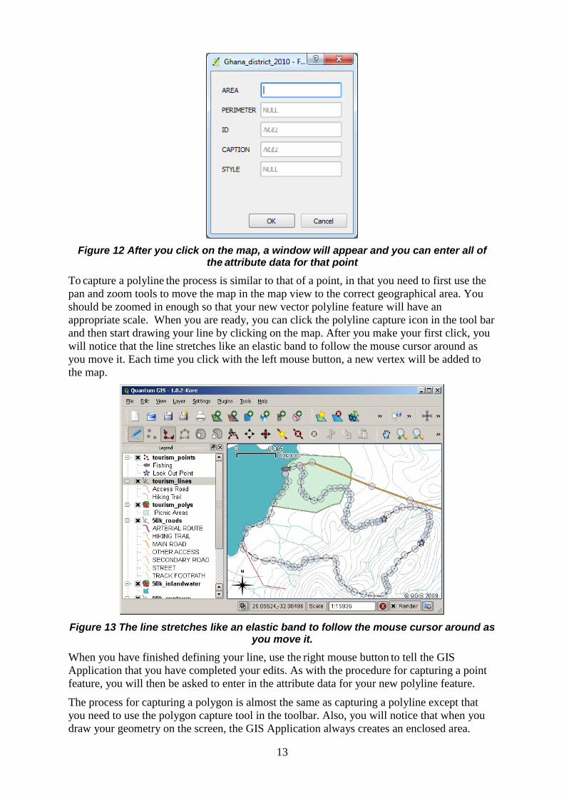
Figure 12 After you click on the map, a window will appear and you can enter all of the attribute data for that point
To capture a polyline the process is similar to that of a point, in that you need to first use the
pan and zoom tools to move the map in the map view to the correct geographical area. You
should be zoomed in enough so that your new vector polyline feature will have an
appropriate scale. When you are ready, you can click the polyline capture icon in the tool bar
and then start drawing your line by clicking on the map. After you make your first click, you
will notice that the line stretches like an elastic band to follow the mouse cursor around as
you move it. Each time you click with the left mouse button, a new vertex will be added to
the map.
Figure 13 The line stretches like an elastic band to follow the mouse cursor around as you move it.
When you have finished defining your line, use the right mouse button to tell the GIS
Application that you have completed your edits. As with the procedure for capturing a poi
feature, you will then be asked to enter in the attribute data for your new polyline feature.
The process for capturing a polygon is almost the same as capturing a polyline except that
you need to use the polygon capture tool in the toolbar. Also, you will notice that when yo
draw your geometry on the screen, the GIS Application always creates an enclosed area.
nt
u

14
To add a new feature after you have created your first one, you can simply click again on the
map with the point, polyline or polygon capture tool active and start to draw your next
feature.
When you have no more features to add, always be sure to click the ‘allow editing’ icon to
toggle it off. The GIS Application will then save your newly created layer to the hard disk.

15
DATA FORMATS AND DATA INTEROPERABILITY
Supported Data Formats
Vector Data Formats
QGIS uses the OGR library to read and write vector data formats, including ESRI shapefiles,
MapInfo and Micro-Station file formats, AutoCAD DXF, PostGIS, SpatiaLite, Oracle Spatial
and MSSQL Spatial databases, and many more. GRASS vector and PostgreSQL support is
supplied by native QGIS data provider plugins. Vector data can also be loaded in read mode
from zip and gzip archives into QGIS
Raster Data formats
QGIS uses the GDAL library to read and write raster data formats, including ArcInfo Binary
Grid, ArcInfo ASCII Grid, GeoTIFF, ERDAS IMAGINE, and many more. GRASS raster
support is supplied by a native QGIS data provider plugin. The raster data can also be loaded
in read mode from zip and gzip archives into QGIS.
Coordinate Systems and data Projections
QGIS has support for approximately 2,700 known CRSs. Definitions for each CRS are stored
in a SQLite database that is installed with QGIS. Normally, you do not need to manipulate
the database directly. In fact, doing so may cause projection support to fail. Custom CRSs are
stored in a user database.
The CRSs available in QGIS are based on those defined by the European Petroleum Search
Group (EPSG) and the Institut Geographique National de France (IGNF) and are largely
abstracted from the spatial reference tables used in GDAL. EPSG identifiers are present in
the database and can be used to specify a CRS in QGIS.
16
PRACTICAL EXERCISE
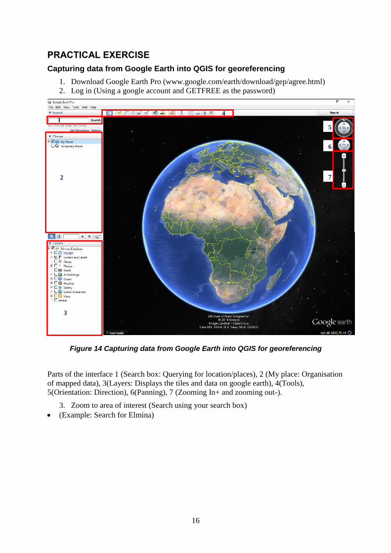
Capturing data from Google Earth into QGIS for georeferencing
1. Download Google Earth Pro (www.google.com/earth/download/gep/agree.html)
2. Log in (Using a google account and GETFREE as the password)
1
2
3
4
7
6
5
Figure 14 Capturing data from Google Earth into QGIS for georeferencing
Parts of the interface 1 (Search box: Querying for location/places), 2 (My place: Organisation
of mapped data), 3(Layers: Displays the tiles and data on google earth), 4(Tools),
5(Orientation: Direction), 6(Panning), 7 (Zooming In+ and zooming out-).
3. Zoom to area of interest (Search using your search box)
(Example: Search for Elmina)

17
Figure 15 Search for Elmina
Explore the image using 6 (Panning), 7 (Zooming) and 5 (Orientation –make sure the
North point is always facing up)
4. Generate control points (which will serve as reference for georeferencing image).
a. Create a folder under My Places (2): Right click on My Places, select Add
and select Folder (Name the folder:Elmina)
b. Right click on the folder created and select Placemark

18
-Type name of point - Change the symbol - Point on photo (Use
pan tool to move the point to the desired location)
c. Repeat, process [ b ] until you get a minimum of 4 points
Figure 16 Generate control points

19
Figure 17 Control points
d. Points should be well over the area of interest (Should be shown on the map
and within your folder [Elmina] under My Places.
5. Save the control points and image
a. Right click on the folder Elmina and select Save Place As
b. Locate a working folder or create one to save the points
6. Save Image
a. Click on File, select Save and select Save Image

20
Figure 18 Save the control points and image
b. Select the highest resolution (Maximum 4800*4074) beside Map Options
c. Click on Save Image (Elmina) and locate a working folder
7. Georeferencing data in QGIS software
a. Open QGIS software
b. Load set the spatial reference of the software environment (Select Settings,
then Options and make sure the coordinate is in the coordinate of the source
data-in this case is World Geodetic Systems WGS1984)

21
Figure 19. Load the Control Points saved from Google Earth
c. Load the Control Points saved from Google Earth
Figure 20 Adding vector
Click Add Vector Click on Browse to locate your add
Change data format to Keyholemarkup Language (Kml)
Select the data (Elmina)
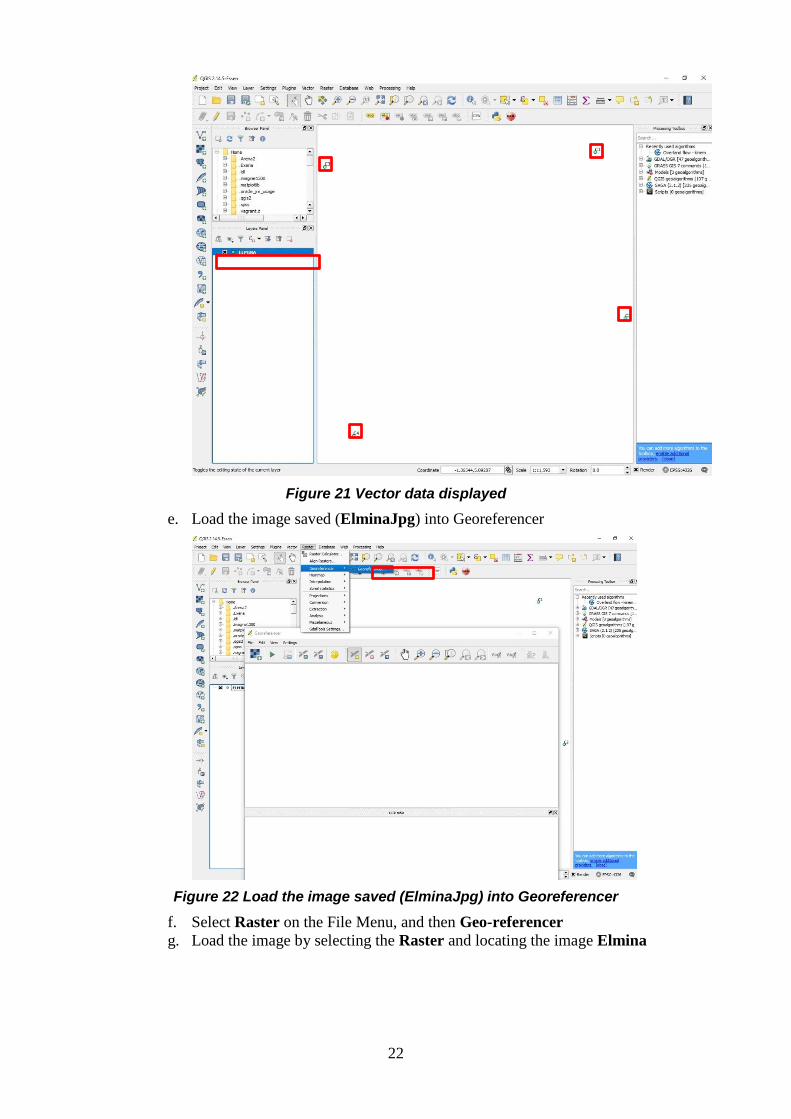
d. Vector data displayed
22
Figure 21 Vector data displayed
e. Load the image saved (ElminaJpg) into Georeferencer
Figure 22 Load the image saved (ElminaJpg) into Georeferencer
f. Select Raster on the File Menu, and then Geo-referencer
g. Load the image by selecting the Raster and locating the image Elmina

23
Figure 23 Load the image by selecting the Raster and locating the image Elmina
Click on Raster tool Select the image
h. Start Georeferencing by adding control points
Figure 24 Start Georeferencing by adding control points
Select Add button Click on the point on the image Select From map
Canvas
i. Select the corresponding point (c3) in the QGIS Data view

24
Figure 25 Select the corresponding point (c3) in the QGIS Data view
j. Ok it on the Enter map Coordinate window. Repeat h and j until all the points
have coordinates
k. Select on settings once all control points on the image has been corresponded
with its vector in the QGIS data view
Figure 26 Click on Play or Run for georeferencing to be effected
l. Click on Play or Run for georeferencing to be effected. (Image is now
georeferenced and it will over lay with the vector data
25
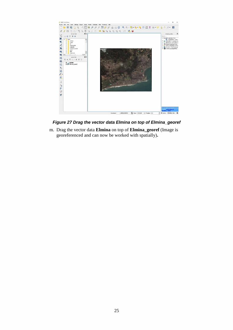
Figure 27 Drag the vector data Elmina on top of Elmina_georef
m. Drag the vector data Elmina on top of Elmina_georef (Image is
georeferenced and can now be worked with spatially).