Manual for microstructure patternrecognition tool

Ondrej Rokos, Vlastimil Kralık

Cech Technical UniversityFaculty of Civil EngineeringDepartment of Structural MechanicsThakurova 7, 166 29 Prague, Czech Republic

September 21, 2012

Contents

1 Introduction 2

2 General notes 2

3 Unpacking 2

4 Running standalone executable gui 24.1 Gui Contour . . . . . . . . . . . . . . . . . . . . . . . . . . . . . . . . . . . 24.2 Gui Mesh . . . . . . . . . . . . . . . . . . . . . . . . . . . . . . . . . . . . 34.3 Gui Solve . . . . . . . . . . . . . . . . . . . . . . . . . . . . . . . . . . . . 5

5 Running source file gui 6

6 Running source mfiles 7

7 Example—aluminium foam 7

1

1 Introduction

Application can be used to characterize the structure of highly porous material. Mechan-ical properties of porous material depends directly on the shape and structure of pores.The obtained geometric parameters (such as distribution of pore walls thicknesses, poresize and shape characteristics) of the highly porous structure are crucial for the selectionof the homogenization schemes and subsequent modeling mechanical performance.

2 General notes

Program is divided into three independent parts CONTOUR, MESH and SOLVE to be usedsequentially or independently.

CONTOUR part serves for pattern recognition in microstructure from image input fileand saves recognized data as *.txt, *.xls, *.mat files. Recognized data includes areamoments of inertia, centroids, etc.

MESH uses previously generated data, decomposes geometry and generates triangularmesh saved in *.mat file.

Plane elasticity problem under boundary conditions is solved in SOLVE part.

3 Unpacking

Downloaded file Data.zip should contain three directories named gui, manual and mfiles.Three ways of running the code are possible: standalone executable gui (graphical userinterface), source files gui, source mfiles (no gui—intended for implementation in user’scode).

Running the code using source files gui or source mfiles requires full installation ofMatlab R©. Standalone executable gui requires free MATLAB Compiler Runtime (MCR),version 7.17 R2012a components which can be downloaded from the web pageshttp://www.mathworks.com/products/compiler/mcr/index.html.

4 Running standalone executable gui

Note: MATLAB Compiler Runtime (MCR), version 7.17 R2012a components should beinstalled first.

Following path Data/gui/executable/win** three files GUI CONTOUR.exe, GUI MESH.exe

and GUI SOLVE.exe are found together with benchmark data example data.jpg. Exe-cutables are compiled for win32 and win64 OS.

4.1 Gui Contour

Graphical interface of GUI CONTOUR.exe is depicted in fig. 1. Window is divided into fourboxes.

Contour data box contains Name of input where input file is to be specified (*.jpg,*.bmp, *.gif, *.tif) and Pixel size which assigns specific length to pixel distances.Program recognizes all contours, but only these with area greater than certain limit areto be taken into account. This limit is specified in Downlimit area. Note that Downlimitarea should consider Pixel size.

2

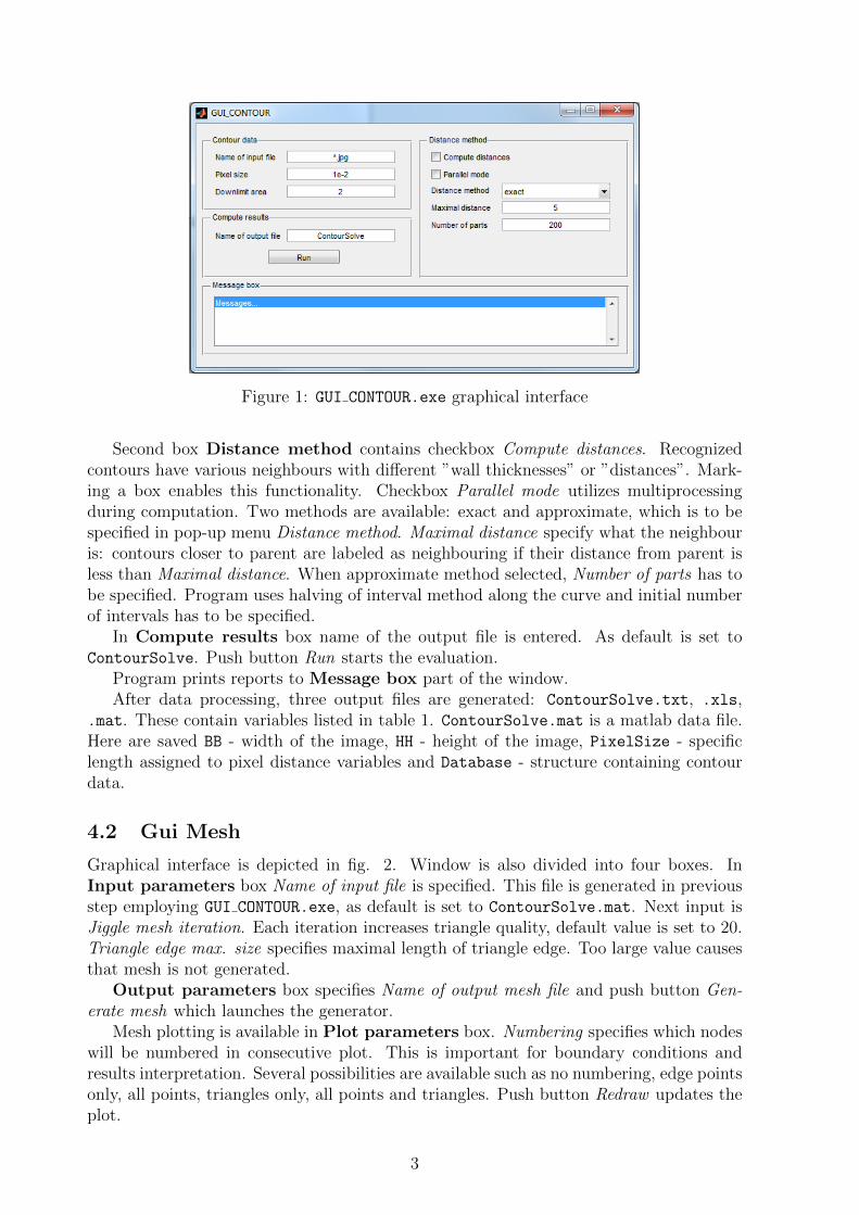
Figure 1: GUI CONTOUR.exe graphical interface

Second box Distance method contains checkbox Compute distances. Recognizedcontours have various neighbours with different ”wall thicknesses” or ”distances”. Mark-ing a box enables this functionality. Checkbox Parallel mode utilizes multiprocessingduring computation. Two methods are available: exact and approximate, which is to bespecified in pop-up menu Distance method. Maximal distance specify what the neighbouris: contours closer to parent are labeled as neighbouring if their distance from parent isless than Maximal distance. When approximate method selected, Number of parts has tobe specified. Program uses halving of interval method along the curve and initial numberof intervals has to be specified.

In Compute results box name of the output file is entered. As default is set toContourSolve. Push button Run starts the evaluation.

Program prints reports to Message box part of the window.After data processing, three output files are generated: ContourSolve.txt, .xls,

.mat. These contain variables listed in table 1. ContourSolve.mat is a matlab data file.Here are saved BB - width of the image, HH - height of the image, PixelSize - specificlength assigned to pixel distance variables and Database - structure containing contourdata.

4.2 Gui Mesh

Graphical interface is depicted in fig. 2. Window is also divided into four boxes. InInput parameters box Name of input file is specified. This file is generated in previousstep employing GUI CONTOUR.exe, as default is set to ContourSolve.mat. Next input isJiggle mesh iteration. Each iteration increases triangle quality, default value is set to 20.Triangle edge max. size specifies maximal length of triangle edge. Too large value causesthat mesh is not generated.

Output parameters box specifies Name of output mesh file and push button Gen-erate mesh which launches the generator.

Mesh plotting is available in Plot parameters box. Numbering specifies which nodeswill be numbered in consecutive plot. This is important for boundary conditions andresults interpretation. Several possibilities are available such as no numbering, edge pointsonly, all points, triangles only, all points and triangles. Push button Redraw updates theplot.

3

Table 1: Variables in output file generated by GUI CONTOUR.exe

Fr. with ratio of inclusion to matrix in the picture with inhomogeneities

Fr. without ratio of inclusion to matrix in the picture without inhomogeneities

ID identification number of area defined by particular contour

Tx x-coordinate of centroid

Ty y-coordinate of centroid

A area circumscribed by particular contour

L circumference of particular contour

Iuu the second centroidal moment of area with respect to x-axis

Ivv the second centroidal moment of area with respect to y-axis

Iuv the product centroidal moment of area with respect to xy-axis

I1 the second moment of area with respect to first principal axis

alpha1 angle between the first principal and x-axis

I2 the second moment of area with respect to second principal axis

alpha2 angle between the second principal and x-axis

J polar area moment of inertia

Figure 2: GUI MESH.exe graphical interface

Program prints reports to Message box part of the window.Mesh parameters are saved in GeneratedMesh.mat file as default. It contains p, e and

t variables which are point, edge and triangle matrices.

4

4.3 Gui Solve

GUI MESH.exe interface is depicted in fig. 3. Input parameters box specifies Mesh inputfile created by GUI MESH.exe and boundary conditions in BC input file. As default is setto bcinput.txt. Example of the file can be found in the same directory or it’s contentsis written below:

Figure 3: GUI SOLVE.exe graphical interface

NodeSupportX = [1313 1312 701 702 52 716 1309:1311 90 717 1301:1308];

NodeSupportY = [1313 1312 701 702 706 1287 708 1288:1290 710 1291:1294

712 1295 1296 697 1252:1265 698 699 1266:1273];

NodeDisplcContrlX = [153 1274:1282 104 1283:1286];

NodeDisplcContrlY = [];

ux = 5;

uy = 0;

NodeForceX = [];

NodeForceY = [];

Fx = 0;

Fy = 0;

Here NodeSupportX specifies nodes supported in X-direction ux = 0, NodeSupportY spec-ifies nodes supported in Y -direction uy = 0, NodeDisplcContrlX specifies nodes withprescribed x-displacements with magnitude ux, NodeDisplcContrlY specifies nodes withprescribed y-displacements with magnitude uy, NodeForceX specifies nodes loaded in x-direction with forces of magnitude Fx, NodeForceY specifies nodes loaded in y-direction

5

with forces of magnitude Fy. Colon operator : is commonly used in Matlab with meaning1283:1286 = 1283 1284 1285 1286.

Solution parameters box specifies as first Solver type. Two possibilities are avail-able: Matlab and Oofem. Oofem solver can be downloaded from web pageshttp://www.oofem.org/en/oofem.html and requires external postprocessor, e.g. ParaView.For this option, oofem.exe file has to be situated in the same folder as GUI SOLVE.exe.Plane mode specifies whether plane strain or plane stress mode will be used. Young’smodulus E, Poisson’s ratio ν are physical parameters of isotropic linear-elastic material,Thickness stands for thickness of the plane object.

Postprocessing box offers Draw pop-up menu where particular components of stressor strain tensors can be selected. Further choice is displacement with scale factor specifiedin Displacement scale input. Push button Redraw updates the plot.

Important messages are printed in Message box.External solver generates several output files, for details see reference web pages (out-

puts are named PdeOofemSolve.out and PdeOofemSolve.vtu). When Matlab solverused, output file PdeMatlabSolve.txt is generated. Data are here structured as follows:

DISPLACEMENTS OUTPUT:

---------------------

Node 1: ux, uy

Node 2: ux, uy

...

ELEMENT OUTPUT:

---------------

Element 1: EpsX, EpsY, EpsZ, GamXY

SigX, SigY, SigZ, TauXY

...

REACTIONS OUTPUT:

-----------------

Node 52: Rx, Ry

Node 90: Rx, Ry

...

Node and triangle labels can be viewed in GUI MESH plot.

5 Running source file gui

Using source files gui requires full installation of Matlab R©. Code is situated in Data/gui/source/,subdirectories GUI CONTOUR, GUI MESH and GUI SOLVE. Graphical interfaces are launchedexecuting GUI CONTOUR.m, GUI MESH.m and GUI SOLVE.m files. Consecutive procedure isthe same as in chapters 4.1, 4.2 and 4.3.

6

6 Running source mfiles

These are intended for implementation in user’s code and full installation of Matlab R© isrequired. Source files are situated in Data/mfiles/ folder. At the beginning of each filenecessary input parameters are specified.

In GUI CONTOUR these are NameInput string, PixelSize, DownlimitArea, ComputeDistances,DistanceMethod, ParallelMode, MaxDist and nParts variables. Meaning of each vari-able can be found in section 4.1.

GUI MESH requires HMax, JiggleIter and Numbering variables, cf. section 4.2.GUI SOLVE then requires PdeMode, PlaneMode variables, material constants EModulus,

Nu, Thickness and boundary conditions NodeSupportX, NodeSupportY, NodeDisplcContrlX,NodeDisplcContrlY, ux, uy, NodeForceX, NodeForceY, Fx and Fy variables. Their de-scription can be found in section 4.3.

File red.m serves for redrawing output data. Typing red + ENTER in Matlab commandline after linear elasticity computation, menu with plot options will appear. matlabSolve.m,oofemSolve.m, minimalDistance.m are supporting functions.

7 Example—aluminium foam

Benchmark example data.jpg can be found in each subfolder. Initial image is depictedin fig. 4 (a). Fully recognized contours can be found in fig 4 (b) emphasized with redcolour. Small inclusions are to be skipped, thus Downlimit area is set to 2. Final solutionis in figure 5. Consecutively, GUI MESH.exe is launched and mesh generated, cf. fig. 6(a). Boundary conditions according to tensile test along x-axis are specified, see 6 (b)and section 4.3 bcinput.txt.

Original image converted to bw and recognized contours

X (1−BB)

Y (

1−H

H)

(a) Input image

Original image converted to bw and recognized contours

X (1−BB)

Y (

1−H

H)

(b) Fully recognized contours

Figure 4: Benchmark example data.jpg

Finally, linear elasticity is solved. All parameters in all three steps are left as default.Deformation with σx stress are depicted if fig. 7 (a), (b). This example primarily servesfor testing correct functionality of the program. Computed results can be compared withdata here introduced.

7

5 10 15 20 25

2

4

6

8

10

12

14

16

Contours used for computation

X (1−BB)

Y (

1−H

H)

1

2

3

4

5

6

7

8

9

10

1112

13

14

Figure 5: Accepted contours

5 10 15 20 25

0

2

4

6

8

10

12

14

16

18

Mesh

X

Y

(a) Mesh

7 8 9 10 11 12 13

−2

−1.5

−1

−0.5

0

0.5

1

1.5

2

2.5

3

Mesh

X

Y 53754

545575556

5775658

75759

75860

6175962

63

64760 1124

532533

534

535112553611265371127

538

539540

5411128542 5435441129545

546 54711305485491131550

551 55211325531133554113411355555561136113755711

168612366871237

69712521253 1254 1255 1256 1257 1258 1259 1260 1261 1262 1263 12641265697 6982214

(b) Mesh—detail

Figure 6: Generated mesh

5 10 15 20 25 30

0

5

10

15

20

X

Y

Deformed mesh

0

0.5

1

1.5

2

2.5

3

3.5

4

4.5

5

(a) Displacement

5 10 15 20 25

0

2

4

6

8

10

12

14

16

18

X

Y

σx

−1000

0

1000

2000

3000

4000

5000

(b) σx

Figure 7: Linear elasticity

8