Embed Size (px)
Citation preview
PSAT
Power System Analysis Toolbox
Documentation for PSAT version 2.0.0 β1, December 14, 2006
Federico Milano

Copyright c© 2003 - 2006 Federico Milano
Permission is granted to copy, distribute and/or modify this document under theterms of the GNU Free Documentation License, Version 1.1 or any later versionpublished by the Free Software Foundation; with the Invariant Sections being allsections, with no Front-Cover Texts, and with no Back-Cover Texts. A copy of thelicense is included in Appendix L entitled “GNU Free Documentation License”.

Ai miei genitori


Note
PSAT is a Matlab toolbox for static and dynamic analysis and control of electricpower systems. I began writing PSAT in September 2001, while I was studying asPh.D. student at the Universita degli Studi di Genova, Italy, and completed the firstpublic version in November 2002, when I was a Visiting Scholar at the University ofWaterloo, Canada. I am currently maintaining PSAT in the spare time, while I amworking as assistant professor at the Universidad de Castilla-La Mancha, CiudadReal, Spain.
PSAT is provided free of charge, in the hope it can be useful and other people can useand improve it, but please be aware that this toolbox comes with ABSOLUTELYNO WARRANTY; for details type warranty at the Matlab prompt. PSAT is freesoftware, and you are welcome to redistribute it under certain conditions; for detailsrefer to Appendix K of this documentation or type gnulicense at the Matlabprompt.
PSAT is currently in a early stage of development and its features, structures anddata formats may be partially or completely changed in future versions. Be sure tovisit often my webpage in order to get the last version:
http://thunderbox.uwaterloo.ca/~fmilano
If you find bugs or have any suggestions, please send me an e-mail at:
or you can subscribe to the PSAT Forum, which is available at:
http://groups.yahoo.com/groups/psatforum

Acknowledgements
I wish to thank very much Professor C. A. Canizares for his priceless help, teachingsand advises. Thanks also for providing me a webpage and a link to my software inthe main webpage of the E&CE Deparment, University of Waterloo, Canada.
Many thanks to the moderators of the PSAT Forum for spending their time onanswering tons of messages: Luigi Vanfretti, Juan Carlos Morataya, Ivo Smon, andZhen Wang.
Thanks to Hugo M. Ayres, Marcelo S. Castro, Alberto Del Rosso, Jasmine, IgorKopcak, Liu Lin, Lars Lindgren, Marcos Miranda, Difahoui Rachid, and SantiagoTorres, for their relevant contributions, corrections and bug fixes.
Contents
I Outlines 1
1 Introduction 3
1.1 Overview . . . . . . . . . . . . . . . . . . . . . . . . . . . . . . . . . 3
1.2 PSAT vs. Other Matlab Toolboxes . . . . . . . . . . . . . . . . . . . 6
1.3 Outlines of the Manual . . . . . . . . . . . . . . . . . . . . . . . . . . 6
1.4 Users . . . . . . . . . . . . . . . . . . . . . . . . . . . . . . . . . . . . 7
2 Getting Started 9
2.1 Download . . . . . . . . . . . . . . . . . . . . . . . . . . . . . . . . . 9
2.2 Requirements . . . . . . . . . . . . . . . . . . . . . . . . . . . . . . . 9
2.3 Installation . . . . . . . . . . . . . . . . . . . . . . . . . . . . . . . . 10
2.4 Launching PSAT . . . . . . . . . . . . . . . . . . . . . . . . . . . . . 11
2.5 Loading Data . . . . . . . . . . . . . . . . . . . . . . . . . . . . . . . 12
2.6 Running the Program . . . . . . . . . . . . . . . . . . . . . . . . . . 14
2.7 Displaying Results . . . . . . . . . . . . . . . . . . . . . . . . . . . . 14
2.8 Saving Results . . . . . . . . . . . . . . . . . . . . . . . . . . . . . . 15
2.9 Settings . . . . . . . . . . . . . . . . . . . . . . . . . . . . . . . . . . 15
2.10 Network Design . . . . . . . . . . . . . . . . . . . . . . . . . . . . . . 16
2.11 Tools . . . . . . . . . . . . . . . . . . . . . . . . . . . . . . . . . . . . 16
2.12 Interfaces . . . . . . . . . . . . . . . . . . . . . . . . . . . . . . . . . 17
3 News 19
3.1 News in version 2.0.0 β1 . . . . . . . . . . . . . . . . . . . . . . . . . 19
3.2 News in version 1.3.4 . . . . . . . . . . . . . . . . . . . . . . . . . . . 20
3.3 News in version 1.3.3 . . . . . . . . . . . . . . . . . . . . . . . . . . . 21
3.4 News in version 1.3.2 . . . . . . . . . . . . . . . . . . . . . . . . . . . 21
3.5 News in version 1.3.1 . . . . . . . . . . . . . . . . . . . . . . . . . . . 21
3.6 News in version 1.3.0 . . . . . . . . . . . . . . . . . . . . . . . . . . . 22
3.7 News in version 1.2.2 . . . . . . . . . . . . . . . . . . . . . . . . . . . 22
3.8 News in version 1.2.1 . . . . . . . . . . . . . . . . . . . . . . . . . . . 23
3.9 News in version 1.2.0 . . . . . . . . . . . . . . . . . . . . . . . . . . . 23
3.10 News in version 1.1.0 . . . . . . . . . . . . . . . . . . . . . . . . . . . 23
3.11 News in version 1.0.1 . . . . . . . . . . . . . . . . . . . . . . . . . . . 23
vii

viii CONTENTS
II Routines 25
4 Power Flow 274.1 Power Flow Solvers . . . . . . . . . . . . . . . . . . . . . . . . . . . . 27
4.1.1 Newton-Raphson Method . . . . . . . . . . . . . . . . . . . . 274.1.2 Fast Decoupled Power Flow . . . . . . . . . . . . . . . . . . . 284.1.3 Distributed Slack Bus Model . . . . . . . . . . . . . . . . . . 294.1.4 Initialization of State Variables . . . . . . . . . . . . . . . . . 30
4.2 Settings . . . . . . . . . . . . . . . . . . . . . . . . . . . . . . . . . . 304.3 Example . . . . . . . . . . . . . . . . . . . . . . . . . . . . . . . . . . 31
5 Bifurcation Analysis 375.1 Direct Methods . . . . . . . . . . . . . . . . . . . . . . . . . . . . . . 38
5.1.1 Saddle-Node Bifurcation . . . . . . . . . . . . . . . . . . . . . 385.1.2 Limit Induced Bifurcation . . . . . . . . . . . . . . . . . . . . 38
5.2 Continuation Power Flow . . . . . . . . . . . . . . . . . . . . . . . . 395.2.1 Predictor Step . . . . . . . . . . . . . . . . . . . . . . . . . . 415.2.2 Corrector Step . . . . . . . . . . . . . . . . . . . . . . . . . . 415.2.3 N-1 Contingency Analysis . . . . . . . . . . . . . . . . . . . . 425.2.4 Graphical User Interface and Settings . . . . . . . . . . . . . 43
5.3 Examples . . . . . . . . . . . . . . . . . . . . . . . . . . . . . . . . . 44
6 Optimal Power Flow 516.1 Interior Point Method . . . . . . . . . . . . . . . . . . . . . . . . . . 516.2 OPF Routines . . . . . . . . . . . . . . . . . . . . . . . . . . . . . . . 52
6.2.1 Maximization of the Social Benefit . . . . . . . . . . . . . . . 526.2.2 Maximization of the Distance to Collapse . . . . . . . . . . . 536.2.3 Multi-Objective Optimization . . . . . . . . . . . . . . . . . . 546.2.4 Lagrangian Function . . . . . . . . . . . . . . . . . . . . . . . 55
6.3 OPF Settings . . . . . . . . . . . . . . . . . . . . . . . . . . . . . . . 556.4 Example . . . . . . . . . . . . . . . . . . . . . . . . . . . . . . . . . . 56
7 Small Signal Stability Analysis 617.1 Small Signal Stability Analysis . . . . . . . . . . . . . . . . . . . . . 61
7.1.1 Example . . . . . . . . . . . . . . . . . . . . . . . . . . . . . . 647.2 QV Sensitivity Analysis . . . . . . . . . . . . . . . . . . . . . . . . . 67
7.2.1 Example . . . . . . . . . . . . . . . . . . . . . . . . . . . . . . 677.3 Graphical User Interface . . . . . . . . . . . . . . . . . . . . . . . . . 70
8 Time Domain Simulation 718.1 Integration Methods . . . . . . . . . . . . . . . . . . . . . . . . . . . 71
8.1.1 Forward Euler Method . . . . . . . . . . . . . . . . . . . . . . 728.1.2 Trapezoidal Method . . . . . . . . . . . . . . . . . . . . . . . 72
8.2 Settings . . . . . . . . . . . . . . . . . . . . . . . . . . . . . . . . . . 728.3 Output Variable Selection . . . . . . . . . . . . . . . . . . . . . . . . 768.4 Snapshots . . . . . . . . . . . . . . . . . . . . . . . . . . . . . . . . . 77

CONTENTS ix
8.5 Disturbances . . . . . . . . . . . . . . . . . . . . . . . . . . . . . . . 798.6 Examples . . . . . . . . . . . . . . . . . . . . . . . . . . . . . . . . . 80
9 PMU Placement 859.1 Linear Static State Estimation . . . . . . . . . . . . . . . . . . . . . 859.2 PMU Placement Rules . . . . . . . . . . . . . . . . . . . . . . . . . . 869.3 Algorithms . . . . . . . . . . . . . . . . . . . . . . . . . . . . . . . . 86
9.3.1 Depth First . . . . . . . . . . . . . . . . . . . . . . . . . . . . 869.3.2 Graph Theoretic Procedure . . . . . . . . . . . . . . . . . . . 879.3.3 Bisecting Search Method . . . . . . . . . . . . . . . . . . . . 879.3.4 Recursive Security N Algorithm . . . . . . . . . . . . . . . . . 879.3.5 Single Shot Security N Algorithm . . . . . . . . . . . . . . . . 889.3.6 Recursive and Single-Shot Security N-1 Algorithms . . . . . . 88
9.4 PMU Placement GUI and Settings . . . . . . . . . . . . . . . . . . . 939.4.1 Example . . . . . . . . . . . . . . . . . . . . . . . . . . . . . . 93
III Models 97
10 Power Flow Data 9910.1 Bus . . . . . . . . . . . . . . . . . . . . . . . . . . . . . . . . . . . . 9910.2 Transmission Line . . . . . . . . . . . . . . . . . . . . . . . . . . . . 10010.3 Transformers . . . . . . . . . . . . . . . . . . . . . . . . . . . . . . . 101
10.3.1 Two-Winding Transformers . . . . . . . . . . . . . . . . . . . 10310.3.2 Three-Winding Transformers . . . . . . . . . . . . . . . . . . 103
10.4 Slack Generator . . . . . . . . . . . . . . . . . . . . . . . . . . . . . . 10410.5 PV Generator . . . . . . . . . . . . . . . . . . . . . . . . . . . . . . . 10610.6 PQ Load . . . . . . . . . . . . . . . . . . . . . . . . . . . . . . . . . . 10710.7 PQ Generator . . . . . . . . . . . . . . . . . . . . . . . . . . . . . . . 10810.8 Shunt . . . . . . . . . . . . . . . . . . . . . . . . . . . . . . . . . . . 10910.9 Area . . . . . . . . . . . . . . . . . . . . . . . . . . . . . . . . . . . . 110
11 CPF and OPF Data 11111.1 Generator Supply . . . . . . . . . . . . . . . . . . . . . . . . . . . . . 11211.2 Generator Reserve . . . . . . . . . . . . . . . . . . . . . . . . . . . . 11311.3 Generator Power Ramping . . . . . . . . . . . . . . . . . . . . . . . . 11411.4 Load Demand . . . . . . . . . . . . . . . . . . . . . . . . . . . . . . . 11511.5 Demand Profile . . . . . . . . . . . . . . . . . . . . . . . . . . . . . . 11611.6 Load Ramping . . . . . . . . . . . . . . . . . . . . . . . . . . . . . . 118
12 Faults & Breakers 12112.1 Fault . . . . . . . . . . . . . . . . . . . . . . . . . . . . . . . . . . . . 12112.2 Breaker . . . . . . . . . . . . . . . . . . . . . . . . . . . . . . . . . . 121
13 Measurements 12513.1 Bus Frequency Measurement . . . . . . . . . . . . . . . . . . . . . . 125

x CONTENTS
13.2 Phasor Measurement Unit . . . . . . . . . . . . . . . . . . . . . . . . 126
14 Loads 12914.1 Voltage Dependent Load . . . . . . . . . . . . . . . . . . . . . . . . . 12914.2 ZIP Load . . . . . . . . . . . . . . . . . . . . . . . . . . . . . . . . . 13014.3 Frequency Dependent Load . . . . . . . . . . . . . . . . . . . . . . . 13214.4 Exponential Recovery Load . . . . . . . . . . . . . . . . . . . . . . . 13314.5 Thermostatically Controlled Load . . . . . . . . . . . . . . . . . . . . 13414.6 Jimma’s Load . . . . . . . . . . . . . . . . . . . . . . . . . . . . . . . 13614.7 Mixed Load . . . . . . . . . . . . . . . . . . . . . . . . . . . . . . . . 13714.8 Note on the Use of Non-conventional Loads . . . . . . . . . . . . . . 138
15 Machines 14115.1 Synchronous Machine . . . . . . . . . . . . . . . . . . . . . . . . . . 141
15.1.1 Order II . . . . . . . . . . . . . . . . . . . . . . . . . . . . . . 14715.1.2 Order III . . . . . . . . . . . . . . . . . . . . . . . . . . . . . 14715.1.3 Order IV . . . . . . . . . . . . . . . . . . . . . . . . . . . . . 14815.1.4 Order V, Type 1 . . . . . . . . . . . . . . . . . . . . . . . . . 14815.1.5 Order V, Type 2 . . . . . . . . . . . . . . . . . . . . . . . . . 14915.1.6 Order V, Type 3 . . . . . . . . . . . . . . . . . . . . . . . . . 14915.1.7 Order VI . . . . . . . . . . . . . . . . . . . . . . . . . . . . . 15015.1.8 Order VIII . . . . . . . . . . . . . . . . . . . . . . . . . . . . 150
15.2 Induction Motor . . . . . . . . . . . . . . . . . . . . . . . . . . . . . 15115.2.1 Order I . . . . . . . . . . . . . . . . . . . . . . . . . . . . . . 15215.2.2 Order III (single cage) . . . . . . . . . . . . . . . . . . . . . . 15315.2.3 Order V (double cage) . . . . . . . . . . . . . . . . . . . . . . 154
16 Controls 15716.1 Turbine Governor . . . . . . . . . . . . . . . . . . . . . . . . . . . . . 157
16.1.1 TG Type I . . . . . . . . . . . . . . . . . . . . . . . . . . . . 15816.1.2 TG Type II . . . . . . . . . . . . . . . . . . . . . . . . . . . . 158
16.2 Automatic Voltage Regulator . . . . . . . . . . . . . . . . . . . . . . 15916.2.1 AVR Type I . . . . . . . . . . . . . . . . . . . . . . . . . . . . 16016.2.2 AVR Type II . . . . . . . . . . . . . . . . . . . . . . . . . . . 16116.2.3 AVR Type III . . . . . . . . . . . . . . . . . . . . . . . . . . . 163
16.3 Power System Stabilizer . . . . . . . . . . . . . . . . . . . . . . . . . 16316.3.1 Type I . . . . . . . . . . . . . . . . . . . . . . . . . . . . . . . 16516.3.2 Type II . . . . . . . . . . . . . . . . . . . . . . . . . . . . . . 16716.3.3 Type III . . . . . . . . . . . . . . . . . . . . . . . . . . . . . . 16716.3.4 Type IV and V . . . . . . . . . . . . . . . . . . . . . . . . . . 168
16.4 Over Excitation Limiter . . . . . . . . . . . . . . . . . . . . . . . . . 16816.5 Secondary Voltage Control . . . . . . . . . . . . . . . . . . . . . . . . 17016.6 Power Oscillation Damper . . . . . . . . . . . . . . . . . . . . . . . . 173
17 Regulating Transformers 17717.1 Under Load Tap Changer . . . . . . . . . . . . . . . . . . . . . . . . 177
CONTENTS xi
17.2 Load Tap Changer With Embedded Load . . . . . . . . . . . . . . . 17817.3 Phase Shifting Transformer . . . . . . . . . . . . . . . . . . . . . . . 182
18 FACTS 18518.1 SVC . . . . . . . . . . . . . . . . . . . . . . . . . . . . . . . . . . . . 18618.2 TCSC . . . . . . . . . . . . . . . . . . . . . . . . . . . . . . . . . . . 18818.3 STATCOM . . . . . . . . . . . . . . . . . . . . . . . . . . . . . . . . 19018.4 SSSC . . . . . . . . . . . . . . . . . . . . . . . . . . . . . . . . . . . . 19318.5 UPFC . . . . . . . . . . . . . . . . . . . . . . . . . . . . . . . . . . . 19618.6 HVDC . . . . . . . . . . . . . . . . . . . . . . . . . . . . . . . . . . . 201
19 Wind Turbines 20519.1 Wind Models . . . . . . . . . . . . . . . . . . . . . . . . . . . . . . . 205
19.1.1 Weibull Distribution . . . . . . . . . . . . . . . . . . . . . . . 20619.1.2 Composite Wind Model . . . . . . . . . . . . . . . . . . . . . 20819.1.3 Measurement Data . . . . . . . . . . . . . . . . . . . . . . . . 209
19.2 Wind Turbines . . . . . . . . . . . . . . . . . . . . . . . . . . . . . . 21019.2.1 Constant Speed Wind Turbine . . . . . . . . . . . . . . . . . 21019.2.2 Doubly Fed Induction Generator . . . . . . . . . . . . . . . . 21319.2.3 Direct Drive Synchronous Generator . . . . . . . . . . . . . . 218
20 Other Models 22320.1 Dynamic Shaft . . . . . . . . . . . . . . . . . . . . . . . . . . . . . . 22320.2 Sub-synchronous Resonance Model . . . . . . . . . . . . . . . . . . . 22520.3 Solid Oxide Fuel Cell . . . . . . . . . . . . . . . . . . . . . . . . . . . 22820.4 Sub-tramsmission Area Equivalents . . . . . . . . . . . . . . . . . . . 233
IV CAD 239
21 Network Design 24121.1 Simulink Library . . . . . . . . . . . . . . . . . . . . . . . . . . . . . 24121.2 Extracting Data from Simulink Models . . . . . . . . . . . . . . . . . 24121.3 Displaying Results in Simulink Models . . . . . . . . . . . . . . . . . 24921.4 Examples . . . . . . . . . . . . . . . . . . . . . . . . . . . . . . . . . 250
22 Block Usage 25522.1 Block Connections . . . . . . . . . . . . . . . . . . . . . . . . . . . . 25522.2 Standard Blocks . . . . . . . . . . . . . . . . . . . . . . . . . . . . . 25622.3 Nonstandard Blocks . . . . . . . . . . . . . . . . . . . . . . . . . . . 258
22.3.1 Buses . . . . . . . . . . . . . . . . . . . . . . . . . . . . . . . 25822.3.2 Goto and From Blocks . . . . . . . . . . . . . . . . . . . . . . 25822.3.3 Links . . . . . . . . . . . . . . . . . . . . . . . . . . . . . . . 25822.3.4 Breakers . . . . . . . . . . . . . . . . . . . . . . . . . . . . . . 25922.3.5 Power Supplies and Demands . . . . . . . . . . . . . . . . . . 26022.3.6 Generator Ramping . . . . . . . . . . . . . . . . . . . . . . . 260

xii CONTENTS
22.3.7 Generator Reserves . . . . . . . . . . . . . . . . . . . . . . . . 26022.3.8 Non-conventional Loads . . . . . . . . . . . . . . . . . . . . . 26022.3.9 Synchronous Machines . . . . . . . . . . . . . . . . . . . . . . 26222.3.10Primary Regulators . . . . . . . . . . . . . . . . . . . . . . . 26322.3.11Secondary Voltage Regulation . . . . . . . . . . . . . . . . . . 26322.3.12Under Load Tap Changers . . . . . . . . . . . . . . . . . . . . 26422.3.13SVCs & STATCOMs . . . . . . . . . . . . . . . . . . . . . . . 26422.3.14Solid Oxide Fuel Cells . . . . . . . . . . . . . . . . . . . . . . 26622.3.15Dynamic Shafts . . . . . . . . . . . . . . . . . . . . . . . . . . 266
23 Block Masks 26923.1 Blocks vs. Global Structures . . . . . . . . . . . . . . . . . . . . . . 26923.2 Editing Block Masks . . . . . . . . . . . . . . . . . . . . . . . . . . . 270
23.2.1 Mask Initialization . . . . . . . . . . . . . . . . . . . . . . . . 27023.2.2 Mask Icon . . . . . . . . . . . . . . . . . . . . . . . . . . . . . 27223.2.3 Mask Documentation . . . . . . . . . . . . . . . . . . . . . . 274
23.3 Syntax of Mask Parameter Names . . . . . . . . . . . . . . . . . . . 27423.4 Remarks on Creating Custom Blocks . . . . . . . . . . . . . . . . . . 275
V Tools 279
24 Data Format Conversion 281
25 User Defined Models 28525.1 Installing and Removing Models . . . . . . . . . . . . . . . . . . . . 28525.2 Creating a User Defined Model . . . . . . . . . . . . . . . . . . . . . 287
25.2.1 Component Settings . . . . . . . . . . . . . . . . . . . . . . . 28725.2.2 State Variable Settings . . . . . . . . . . . . . . . . . . . . . . 29125.2.3 Parameter Settings . . . . . . . . . . . . . . . . . . . . . . . . 292
25.3 Limitations . . . . . . . . . . . . . . . . . . . . . . . . . . . . . . . . 292
26 Utilities 29326.1 Command History . . . . . . . . . . . . . . . . . . . . . . . . . . . . 29326.2 Sparse Matrix Visualization . . . . . . . . . . . . . . . . . . . . . . . 29326.3 Themes . . . . . . . . . . . . . . . . . . . . . . . . . . . . . . . . . . 29326.4 Text Viewer . . . . . . . . . . . . . . . . . . . . . . . . . . . . . . . . 29326.5 Building p-code Archive . . . . . . . . . . . . . . . . . . . . . . . . . 294
27 Command Line Usage 29927.1 Basics . . . . . . . . . . . . . . . . . . . . . . . . . . . . . . . . . . . 29927.2 Advanced Usage . . . . . . . . . . . . . . . . . . . . . . . . . . . . . 30227.3 Command Line Options . . . . . . . . . . . . . . . . . . . . . . . . . 30327.4 Example . . . . . . . . . . . . . . . . . . . . . . . . . . . . . . . . . . 304
28 Running PSAT on GNU Octave 30728.1 Basic Commands . . . . . . . . . . . . . . . . . . . . . . . . . . . . . 308
CONTENTS xiii
28.2 Plot Variables . . . . . . . . . . . . . . . . . . . . . . . . . . . . . . . 30828.3 ToDos . . . . . . . . . . . . . . . . . . . . . . . . . . . . . . . . . . . 310
VI Interfaces 311
29 GAMS Interface 31329.1 Getting Started . . . . . . . . . . . . . . . . . . . . . . . . . . . . . . 31329.2 GAMS Solvers . . . . . . . . . . . . . . . . . . . . . . . . . . . . . . 31429.3 PSAT-GAMS Interface . . . . . . . . . . . . . . . . . . . . . . . . . . 31429.4 PSAT-GAMS Models . . . . . . . . . . . . . . . . . . . . . . . . . . . 31529.5 Multiperiod Market Clearing Model . . . . . . . . . . . . . . . . . . 318
29.5.1 Notation . . . . . . . . . . . . . . . . . . . . . . . . . . . . . . 31829.5.2 Model Equations and Constraints . . . . . . . . . . . . . . . . 319
29.6 Example . . . . . . . . . . . . . . . . . . . . . . . . . . . . . . . . . . 321
30 UWPFLOW Interface 32930.1 Getting Started . . . . . . . . . . . . . . . . . . . . . . . . . . . . . . 32930.2 Graphical User Interface . . . . . . . . . . . . . . . . . . . . . . . . . 33030.3 Limitations and ToDos . . . . . . . . . . . . . . . . . . . . . . . . . . 33030.4 Example . . . . . . . . . . . . . . . . . . . . . . . . . . . . . . . . . . 332
VII Libraries 337
31 Numeric Linear Analysis 33931.1 Description . . . . . . . . . . . . . . . . . . . . . . . . . . . . . . . . 33931.2 Test cases . . . . . . . . . . . . . . . . . . . . . . . . . . . . . . . . . 340
31.2.1 Comparison of state matrices . . . . . . . . . . . . . . . . . . 34131.2.2 Results for a change of an exciter reference voltage . . . . . . 34131.2.3 Results for a change of governor reference speeds . . . . . . . 34231.2.4 Results for a change of a SVC reference voltage . . . . . . . . 345
VIII Appendices 349
A Global Structures & Classes 351A.1 General Settings . . . . . . . . . . . . . . . . . . . . . . . . . . . . . 351A.2 Other Settings . . . . . . . . . . . . . . . . . . . . . . . . . . . . . . 355A.3 System Properties and Settings . . . . . . . . . . . . . . . . . . . . . 357A.4 Outputs and Variable Names . . . . . . . . . . . . . . . . . . . . . . 364A.5 User Defined Models . . . . . . . . . . . . . . . . . . . . . . . . . . . 364A.6 Models . . . . . . . . . . . . . . . . . . . . . . . . . . . . . . . . . . . 366A.7 Command Line Usage . . . . . . . . . . . . . . . . . . . . . . . . . . 368A.8 Interfaces . . . . . . . . . . . . . . . . . . . . . . . . . . . . . . . . . 369A.9 Classes . . . . . . . . . . . . . . . . . . . . . . . . . . . . . . . . . . . 370
xiv CONTENTS
B Matlab Functions 373
C Other Files and Folders 381
D Third Party Matlab Code 385
E Power System Softwares 387
F Test System Data 389F.1 3-bus Test System . . . . . . . . . . . . . . . . . . . . . . . . . . . . 389F.2 6-bus Test System . . . . . . . . . . . . . . . . . . . . . . . . . . . . 390F.3 9-bus Test System . . . . . . . . . . . . . . . . . . . . . . . . . . . . 391F.4 14-bus Test System . . . . . . . . . . . . . . . . . . . . . . . . . . . . 394
G FAQs 397G.1 Getting Started . . . . . . . . . . . . . . . . . . . . . . . . . . . . . . 397G.2 Simulink Library . . . . . . . . . . . . . . . . . . . . . . . . . . . . . 399G.3 Power Flow . . . . . . . . . . . . . . . . . . . . . . . . . . . . . . . . 400G.4 Optimal & Continuation Power Flow . . . . . . . . . . . . . . . . . . 401G.5 Time Domain Simulation . . . . . . . . . . . . . . . . . . . . . . . . 401G.6 Data Conversion . . . . . . . . . . . . . . . . . . . . . . . . . . . . . 402G.7 Interfaces . . . . . . . . . . . . . . . . . . . . . . . . . . . . . . . . . 403
H PSAT Forum 405
I References & Links 409I.1 Books . . . . . . . . . . . . . . . . . . . . . . . . . . . . . . . . . . . 409I.2 Journals . . . . . . . . . . . . . . . . . . . . . . . . . . . . . . . . . . 409I.3 Conference Proceedings . . . . . . . . . . . . . . . . . . . . . . . . . 410I.4 Webpages . . . . . . . . . . . . . . . . . . . . . . . . . . . . . . . . . 410
J Recommendation Letters 413
K The GNU General Public License 435
L GNU Free Documentation License 443
Bibliography 450
Index 461

List of Figures
1.1 PSAT at a glance. . . . . . . . . . . . . . . . . . . . . . . . . . . . 51.2 PSAT around the world. . . . . . . . . . . . . . . . . . . . . . . . . 8
2.1 Main graphical user interface of PSAT. . . . . . . . . . . . . . . . 13
4.1 GUI for general settings. . . . . . . . . . . . . . . . . . . . . . . . . 324.2 GUI for displaying power flow results. . . . . . . . . . . . . . . . . 33
5.1 GUI for saddle-node bifurcation settings. . . . . . . . . . . . . . . 395.2 GUI for limit-induced bifurcation settings. . . . . . . . . . . . . . . 405.3 Continuation Power Flow: tangent vector . . . . . . . . . . . . . . 415.4 Continuation Power Flow: perpendicular intersection . . . . . . . . 425.5 Continuation Power Flow: local parametrization . . . . . . . . . . 435.6 GUI for the continuation power flow settings. . . . . . . . . . . . . 455.7 GUI for plotting CPF results. . . . . . . . . . . . . . . . . . . . . . 465.8 Nose curves for the 6-bus test system (LIB) . . . . . . . . . . . . . 475.9 Nose curves for the 6-bus test system (SNB) . . . . . . . . . . . . 48
6.1 GUI for the optimal power flow. . . . . . . . . . . . . . . . . . . . 566.2 GUI for displaying OPF results. . . . . . . . . . . . . . . . . . . . 576.3 GUI for plotting OPF Pareto sets. . . . . . . . . . . . . . . . . . . 60
7.1 Eigenvalue Analysis: S-domain. . . . . . . . . . . . . . . . . . . . . 637.2 Eigenvalue Analysis: Z-domain. . . . . . . . . . . . . . . . . . . . 637.3 Eigenvalue Analysis: QV sensitivity. . . . . . . . . . . . . . . . . . 687.4 GUI for the small signal stability analysis. . . . . . . . . . . . . . . 70
8.1 Time domain integration block diagram. . . . . . . . . . . . . . . . 738.2 GUI for general settings. . . . . . . . . . . . . . . . . . . . . . . . . 758.3 GUI for plot variable selection. . . . . . . . . . . . . . . . . . . . . 788.4 Snapshot GUI. . . . . . . . . . . . . . . . . . . . . . . . . . . . . . 798.5 GUI for plotting time domain simulations. . . . . . . . . . . . . . . 818.6 Generator speeds for the 9-bus test system. . . . . . . . . . . . . . 828.7 Generator rotor angles for the 9-bus test system. . . . . . . . . . . 838.8 Bus voltages for the 9-bus test system. . . . . . . . . . . . . . . . . 84
9.1 PMU placement rules. . . . . . . . . . . . . . . . . . . . . . . . . . 87
xv

xvi LIST OF FIGURES
9.2 Flowchart of the Graph Theoretic Procedure. . . . . . . . . . . . . 889.3 Flowchart of the Bisecting Search. . . . . . . . . . . . . . . . . . . 899.4 Pseudo-code of the simulated Annealing Algorithm. . . . . . . . . 909.5 Recursive N Security Method. . . . . . . . . . . . . . . . . . . . . . 919.6 Search of alternative placement sets. . . . . . . . . . . . . . . . . . 919.7 Pure transit node filtering. . . . . . . . . . . . . . . . . . . . . . . 919.8 Single-Shot N Security Method. . . . . . . . . . . . . . . . . . . . . 929.9 Recursive N-1 Security Method. . . . . . . . . . . . . . . . . . . . 939.10 Single Shot N-1 Security Method. . . . . . . . . . . . . . . . . . . 949.11 GUI for the PMU placement methods. . . . . . . . . . . . . . . . . 95
10.1 Transmission line π circuit. . . . . . . . . . . . . . . . . . . . . . . 10110.2 Three-winding transformer equivalent circuit. . . . . . . . . . . . . 104
11.1 Example of daily demand profile. . . . . . . . . . . . . . . . . . . . 119
13.1 Bus frequency measurement filter. . . . . . . . . . . . . . . . . . . 12513.2 Phasors from sample data. . . . . . . . . . . . . . . . . . . . . . . 127
14.1 Measure of frequency deviation. . . . . . . . . . . . . . . . . . . . . 13214.2 Thermostatically controlled load. . . . . . . . . . . . . . . . . . . . 13514.3 Jimma’s load. . . . . . . . . . . . . . . . . . . . . . . . . . . . . . . 137
15.1 Synchronous machine scheme. . . . . . . . . . . . . . . . . . . . . . 14215.2 Synchronous machine: block diagram of stator fluxes. . . . . . . . 14315.3 Field saturation characteristic of synchronous machines. . . . . . . 14415.4 Order I induction motor: electrical circuit. . . . . . . . . . . . . . 15415.5 Order III induction motor: electrical circuit. . . . . . . . . . . . . 15415.6 Order V induction motor: electrical circuit. . . . . . . . . . . . . . 155
16.1 Turbine governor type I. . . . . . . . . . . . . . . . . . . . . . . . . 15816.2 Turbine governor type II. . . . . . . . . . . . . . . . . . . . . . . . 15916.3 Exciter Type I. . . . . . . . . . . . . . . . . . . . . . . . . . . . . . 16116.4 Exciter Type II. . . . . . . . . . . . . . . . . . . . . . . . . . . . . 16216.5 Exciter Type III. . . . . . . . . . . . . . . . . . . . . . . . . . . . . 16416.6 Power system stabilizer Type I. . . . . . . . . . . . . . . . . . . . . 16716.7 Power system stabilizer Type II. . . . . . . . . . . . . . . . . . . . 16716.8 Power system stabilizer Type III. . . . . . . . . . . . . . . . . . . . 16816.9 Power system stabilizer Type IV. . . . . . . . . . . . . . . . . . . . 16916.10 Power system stabilizer Type V. . . . . . . . . . . . . . . . . . . . 16916.11 Over excitation limiter. . . . . . . . . . . . . . . . . . . . . . . . . 17116.12 Secondary voltage control scheme. . . . . . . . . . . . . . . . . . . 172
17.1 Under Load Tap Changer: equivalent π circuit. . . . . . . . . . . . 17917.2 Under Load Tap Changer: voltage and reactive power controls. . . 17917.3 Load Tap Changer with embedded load. . . . . . . . . . . . . . . . 18117.4 Phase shifting transformer circuit. . . . . . . . . . . . . . . . . . . 182
LIST OF FIGURES xvii
17.5 Phase shifting transformer control scheme. . . . . . . . . . . . . . 183
18.1 SVC Type 1 Regulator. . . . . . . . . . . . . . . . . . . . . . . . . 18618.2 SVC Type 2 Regulator. . . . . . . . . . . . . . . . . . . . . . . . . 187
18.3 TCSC Regulator. . . . . . . . . . . . . . . . . . . . . . . . . . . . . 189
18.4 STATCOM circuit and control block diagram. . . . . . . . . . . . 19218.5 SSSC circuit. . . . . . . . . . . . . . . . . . . . . . . . . . . . . . . 194
18.6 SSSC control block diagram. . . . . . . . . . . . . . . . . . . . . . 195
18.7 UPFC circuit. . . . . . . . . . . . . . . . . . . . . . . . . . . . . . . 19818.8 UPFC phasor diagram. . . . . . . . . . . . . . . . . . . . . . . . . 198
18.9 UPFC control block diagrams. . . . . . . . . . . . . . . . . . . . . 199
18.10 HVDC current control. . . . . . . . . . . . . . . . . . . . . . . . . 202
19.1 Low-pass filter to smooth wind speed variations. . . . . . . . . . . 206
19.2 Wind turbine types . . . . . . . . . . . . . . . . . . . . . . . . . . 211
19.3 Rotor speed control scheme. . . . . . . . . . . . . . . . . . . . . . . 217
19.4 Voltage control scheme. . . . . . . . . . . . . . . . . . . . . . . . . 21719.5 Power-speed characteristic. . . . . . . . . . . . . . . . . . . . . . . 217
19.6 Pitch angle control scheme. . . . . . . . . . . . . . . . . . . . . . . 218
20.1 Synchronous machine mass-spring shaft model. . . . . . . . . . . . 22420.2 Generator with dynamic shaft and compensated line. . . . . . . . . 226
20.3 Solid Oxide Fuel Cell scheme. . . . . . . . . . . . . . . . . . . . . . 231
20.4 Solid Oxide Fuel Cell connection with the AC grid. . . . . . . . . . 23320.5 AC voltage control for the Solid Oxide Fuel Cell. . . . . . . . . . . 233
20.6 Sub-transmission equivalent area. . . . . . . . . . . . . . . . . . . . 236
21.1 Simulink library: Main Window. . . . . . . . . . . . . . . . . . . . 24221.2 Simulink library: Connections. . . . . . . . . . . . . . . . . . . . . 242
21.3 Simulink library: Power Flow data. . . . . . . . . . . . . . . . . . . 243
21.4 Simulink library: OPF & CPF data. . . . . . . . . . . . . . . . . . 244
21.5 Simulink library: Faults & Breakers. . . . . . . . . . . . . . . . . . 24421.6 Simulink library: Measurements. . . . . . . . . . . . . . . . . . . . 244
21.7 Simulink library: Loads. . . . . . . . . . . . . . . . . . . . . . . . . 245
21.8 Simulink library: Machines. . . . . . . . . . . . . . . . . . . . . . . 24521.9 Simulink library: Regulators. . . . . . . . . . . . . . . . . . . . . . 246
21.10 Simulink library: Regulating Transformers. . . . . . . . . . . . . . 246
21.11 Simulink library: FACTS controllers. . . . . . . . . . . . . . . . . . 24721.12 Simulink library: Wind Turbines. . . . . . . . . . . . . . . . . . . . 248
21.13 Simulink library: Other models. . . . . . . . . . . . . . . . . . . . 248
21.14 Simulink library: Subtransmission equivalent areas. . . . . . . . . 249
21.15 GUI for Simulink model settings. . . . . . . . . . . . . . . . . . . . 25021.16 Simulink model of the WSCC 3-generator 9-bus test system. . . . 251
21.17 Simulink model of the IEEE 14-bus test system. . . . . . . . . . . 252
21.18 Simulink model of the 6-bus test system. . . . . . . . . . . . . . . 253
xviii LIST OF FIGURES
22.1 Examples of standard blocks of the PSAT Simulink Library. . . . 25622.2 Examples of allowed connections. . . . . . . . . . . . . . . . . . . . 25722.3 Examples of not allowed connections. . . . . . . . . . . . . . . . . 25722.4 Examples of infeasible connections. . . . . . . . . . . . . . . . . . . 25722.5 Bus block usage. . . . . . . . . . . . . . . . . . . . . . . . . . . . . 25822.6 Goto and From block usage. . . . . . . . . . . . . . . . . . . . . . . 25922.7 Breaker block usage. . . . . . . . . . . . . . . . . . . . . . . . . . . 25922.8 Supply and Demand block usage. . . . . . . . . . . . . . . . . . . . 26022.9 Generator Ramping block usage. . . . . . . . . . . . . . . . . . . . 26122.10 Generator Reserve block usage. . . . . . . . . . . . . . . . . . . . . 26122.11 Non-conventional Load block usage. . . . . . . . . . . . . . . . . . 26222.12 Synchronous Machine block usage. . . . . . . . . . . . . . . . . . . 26322.13 Primary Regulator block usage. . . . . . . . . . . . . . . . . . . . . 26422.14 Secondary Voltage Regulation block usage. . . . . . . . . . . . . . 26522.15 Under Load Tap Changer block usage. . . . . . . . . . . . . . . . . 26522.16 SVC block usage. . . . . . . . . . . . . . . . . . . . . . . . . . . . . 26622.17 Solid Oxide Fuel Cell block usage. . . . . . . . . . . . . . . . . . . 26622.18 Dynamic Shaft block usage. . . . . . . . . . . . . . . . . . . . . . . 267
23.1 Simulink blocks vs. PSAT global structures . . . . . . . . . . . . 27023.2 Mask GUI of a PSAT-Simulink block. . . . . . . . . . . . . . . . 27123.3 Mask initialization GUI for a PSAT-Simulink block. . . . . . . . 27223.4 Mask icon GUI of a PSAT-Simulink block. . . . . . . . . . . . . . 27323.5 Mask documentation GUI of a PSAT-Simulink block. . . . . . . . 27423.6 Simulink model underneath a mask of a PSAT block. . . . . . . . 277
24.1 GUI for data format conversion. . . . . . . . . . . . . . . . . . . . 283
25.1 Browser of user defined models. . . . . . . . . . . . . . . . . . . . . 28625.2 GUI for creating user defined models. . . . . . . . . . . . . . . . . 28825.3 GUI for setting component properties. . . . . . . . . . . . . . . . . 28925.4 GUI for setting state variable properties. . . . . . . . . . . . . . . 29025.5 GUI for setting parameters properties. . . . . . . . . . . . . . . . . 291
26.1 Command history GUI. . . . . . . . . . . . . . . . . . . . . . . . . 29426.2 GUI for sparse matrix visualization. . . . . . . . . . . . . . . . . . 29526.3 GUI for PSAT theme selection. . . . . . . . . . . . . . . . . . . . . 29626.4 GUI for text viewer selection. . . . . . . . . . . . . . . . . . . . . . 29726.5 GUI for p-code archive builder. . . . . . . . . . . . . . . . . . . . . 297
27.1 Master-slave architecture. . . . . . . . . . . . . . . . . . . . . . . . 302
28.1 Example of graph obtained using GNU/Octave and gplot. . . . . . 309
29.1 Structure of the PSAT-GAMS interface. . . . . . . . . . . . . . . . 31629.2 GUI of the PSAT-GAMS interface. . . . . . . . . . . . . . . . . . . 31729.3 PSAT-Simulink model of the three-bus test system. . . . . . . . . 323

LIST OF FIGURES xix
29.4 Demand profile for the multiperiod auction. . . . . . . . . . . . . . 32329.5 Multiperiod auction without Pmax
mn limits. . . . . . . . . . . . . . . 32729.6 Multiperiod auction with Pmax
mn limits. . . . . . . . . . . . . . . . . 328
30.1 GUI of the PSAT-UWPFLOW interface. . . . . . . . . . . . . . . 33130.2 UWPFLOW nose curves for the 6-bus test systems. . . . . . . . . 336
31.1 Comparison of voltages at buses 6 and 7. . . . . . . . . . . . . . . 34331.2 Comparison of reactive powers flows in lines 2-7 and 6-4. . . . . . 34331.3 Comparison of active powers flows in line 2-7. . . . . . . . . . . . . 34431.4 Comparison of rotor speeds. . . . . . . . . . . . . . . . . . . . . . . 34631.5 Detail of the comparison of rotor speeds. . . . . . . . . . . . . . . 34631.6 Comparison of active powers flows in line 2-7. . . . . . . . . . . . . 34731.7 Comparison of SVC state variables. . . . . . . . . . . . . . . . . . 34831.8 Comparison of voltages at bus 8. . . . . . . . . . . . . . . . . . . . 348
F.1 3-bus test system. . . . . . . . . . . . . . . . . . . . . . . . . . . . 390F.2 6-bus test system. . . . . . . . . . . . . . . . . . . . . . . . . . . . 392F.3 WSCC 3-generator 9-bus test system. . . . . . . . . . . . . . . . . 394F.4 IEEE 14-bus test system. . . . . . . . . . . . . . . . . . . . . . . . 396
H.1 PSAT Forum main page . . . . . . . . . . . . . . . . . . . . . . . . 406H.2 PSAT Forum statistics . . . . . . . . . . . . . . . . . . . . . . . . . 407

List of Tables
1.1 Matlab-based packages for power system analysis . . . . . . . . . . 6
5.1 N-1 Contingency Analysis Report . . . . . . . . . . . . . . . . . . 49
10.1 Bus Data Format . . . . . . . . . . . . . . . . . . . . . . . . . . . . 9910.2 Line Data Format . . . . . . . . . . . . . . . . . . . . . . . . . . . 10210.3 Alternative Line Data Format . . . . . . . . . . . . . . . . . . . . . 10210.4 Transformer Data Format . . . . . . . . . . . . . . . . . . . . . . . 10310.5 Three-Winding Transformer Data Format . . . . . . . . . . . . . . 10510.6 Slack Generator Data Format . . . . . . . . . . . . . . . . . . . . . 10510.7 PV Generator Data Format . . . . . . . . . . . . . . . . . . . . . . 10710.8 PQ Load Data Format . . . . . . . . . . . . . . . . . . . . . . . . . 10810.9 PQ Generator Data Format . . . . . . . . . . . . . . . . . . . . . . 10910.10 Shunt Admittance Data Format . . . . . . . . . . . . . . . . . . . 10910.11 Area Data Format . . . . . . . . . . . . . . . . . . . . . . . . . . . 110
11.1 Power Supply Data Format . . . . . . . . . . . . . . . . . . . . . . 11311.2 Power Reserve Data Format . . . . . . . . . . . . . . . . . . . . . . 11411.3 Generator Power Ramping Data Format . . . . . . . . . . . . . . . 11511.4 Power Demand Data Format . . . . . . . . . . . . . . . . . . . . . 11711.5 Demand Profile Data Format . . . . . . . . . . . . . . . . . . . . . 11911.6 Load Ramping Data Format . . . . . . . . . . . . . . . . . . . . . 120
12.1 Fault Data Format . . . . . . . . . . . . . . . . . . . . . . . . . . . 12212.2 Breaker Data Format . . . . . . . . . . . . . . . . . . . . . . . . . 123
13.1 Bus Frequency Measurement Data Format . . . . . . . . . . . . . . 12613.2 Phasor Measurement Unit Data Format . . . . . . . . . . . . . . . 128
14.1 Voltage Dependent Load Data Format . . . . . . . . . . . . . . . . 13014.2 ZIP Load Data Format . . . . . . . . . . . . . . . . . . . . . . . . 13114.3 Frequency Dependent Load Data Format . . . . . . . . . . . . . . 13314.4 Typical load coefficients . . . . . . . . . . . . . . . . . . . . . . . . 13314.5 Exponential Recovery Load Data Format . . . . . . . . . . . . . . 13414.6 Thermostatically Controlled Load Data Format . . . . . . . . . . . 13614.7 Jimma’s Load Data Format . . . . . . . . . . . . . . . . . . . . . . 137
xx
LIST OF TABLES xxi
14.8 Mixed Load Data Format . . . . . . . . . . . . . . . . . . . . . . . 139
15.1 Synchronous Machine Data Format . . . . . . . . . . . . . . . . . . 14615.2 Reference table for synchronous machine parameters. . . . . . . . . 14715.3 Induction Motor Data Format . . . . . . . . . . . . . . . . . . . . 153
16.1 Turbine Governor Type I Data Format . . . . . . . . . . . . . . . . 15916.2 Turbine Governor Type II Data Format . . . . . . . . . . . . . . . 16016.3 Exciter Type I Data Format . . . . . . . . . . . . . . . . . . . . . 16216.4 Exciter Type II Data Format . . . . . . . . . . . . . . . . . . . . . 16316.5 Exciter Type III Data Format . . . . . . . . . . . . . . . . . . . . 16416.6 Power System Stabilizer Data Format . . . . . . . . . . . . . . . . 16616.7 Over Excitation Limiter Data Format . . . . . . . . . . . . . . . . 17116.8 Central Area Controller Data Format . . . . . . . . . . . . . . . . 17316.9 Cluster Controller Data Format . . . . . . . . . . . . . . . . . . . . 17416.10 Power Oscillation Damper Data Format . . . . . . . . . . . . . . . 175
17.1 Load Tap Changer Data Format . . . . . . . . . . . . . . . . . . . 18017.2 Tap Changer with Embedded Load Data Format . . . . . . . . . . 18117.3 Phase Shifting Transformer Data Format . . . . . . . . . . . . . . 183
18.1 SVC Type 1 Data Format . . . . . . . . . . . . . . . . . . . . . . . 18718.2 SVC Type 2 Data Format . . . . . . . . . . . . . . . . . . . . . . . 18818.3 TCSC Data Format . . . . . . . . . . . . . . . . . . . . . . . . . . 19118.4 STATCOM Data Format . . . . . . . . . . . . . . . . . . . . . . . 19218.5 SSSC Data Format . . . . . . . . . . . . . . . . . . . . . . . . . . . 19518.6 UPFC Data Format . . . . . . . . . . . . . . . . . . . . . . . . . . 20018.7 HVDC Data Format . . . . . . . . . . . . . . . . . . . . . . . . . . 203
19.1 Wind Speed Data Format . . . . . . . . . . . . . . . . . . . . . . . 20719.2 Roughness length for various ground surfaces . . . . . . . . . . . . 20919.3 Recent wind turbines . . . . . . . . . . . . . . . . . . . . . . . . . 21019.4 Constant Speed Wind Turbine Data Format . . . . . . . . . . . . . 21419.5 Doubly Fed Induction Generator Data Format . . . . . . . . . . . 21919.6 Direct Drive Synchronous Generator Data Format . . . . . . . . . 222
20.1 Dynamic Shaft Data Format . . . . . . . . . . . . . . . . . . . . . 22520.2 SSR Data Format . . . . . . . . . . . . . . . . . . . . . . . . . . . 22920.3 Solid Oxide Fuel Cell Data Format . . . . . . . . . . . . . . . . . . 23220.4 Sub-transmission Area (2 loads) Data Format . . . . . . . . . . . . 23720.5 Sub-transmission Area (3 loads) Data Format . . . . . . . . . . . . 238
23.1 Mask parameter symbols . . . . . . . . . . . . . . . . . . . . . . . 27523.2 Example of well formed mask variable names . . . . . . . . . . . . 27523.3 Mask parameter constants . . . . . . . . . . . . . . . . . . . . . . . 276
25.1 Functions and files to be modified for installing a UDM . . . . . . 285

xxii LIST OF TABLES
27.1 Routine Conventional Names for Command Line Usage. . . . . . . 30127.2 General Options for Command Line Usage. . . . . . . . . . . . . . 30227.3 Structures to be modified to change default behavior. . . . . . . . 303
29.1 PSAT IPM-based OPF report for the three-bus test system. . . . . 32429.2 PSAT-GAMS OPF report for the three-bus test system. . . . . . . 32529.3 Input file psatglobs.gms for the three-bus test system. . . . . . . 32529.4 Input file psatdata.gms for the three-bus test system. . . . . . . . 32629.5 Output file psatsol.m for the three-bus test system. . . . . . . . . 326
30.1 IEEE CDF file to be used within UWPFLOW . . . . . . . . . . . 33330.2 UWPFLOW power flow results . . . . . . . . . . . . . . . . . . . . 33430.3 Input file which defines power directions in UWPFLOW . . . . . . 33530.4 UWPFLOW output file with CPF results . . . . . . . . . . . . . . 335
31.1 State matrix eigenvalues for the 9-bus test system . . . . . . . . . 341

Part I
Outlines

Chapter 1
Introduction
This chapter provides an overview of PSAT features and a comparison with otherMatlab toolboxes for power system analysis. The outlines of this documentationand a list of PSAT users around the world are also reported.
1.1 Overview
PSAT is a Matlab toolbox for electric power system analysis and control. Thecommand line version of PSAT is also GNU Octave compatible. PSAT includespower flow, continuation power flow, optimal power flow, small signal stabilityanalysis and time domain simulation. All operations can be assessed by means ofgraphical user interfaces (GUIs) and a Simulink-based library provides an userfriendly tool for network design.
PSAT core is the power flow routine, which also takes care of state variableinitialization. Once the power flow has been solved, further static and/or dynamicanalysis can be performed. These routines are:
1. Continuation power flow;
2. Optimal power flow;
3. Small signal stability analysis;
4. Time domain simulations;
5. Phasor measurement unit (PMU) placement.
In order to perform accurate power system analysis, PSAT supports a variety ofstatic and dynamic component models, as follows:
Power Flow Data: Bus bars, transmission lines and transformers, slack buses, PVgenerators, constant power loads, and shunt admittances.
CPF and OPF Data: Power supply bids and limits, generator power reserves,generator ramping data, and power demand bids and limits.
3

4 1 Introduction
Switching Operations: Transmission line faults and transmission line breakers.
Measurements: Bus frequency and phasor measurement units (PMU).
Loads: Voltage dependent loads, frequency dependent loads, ZIP (impedance,constant current and constant power) loads, exponential recovery loads [Hill1993, Karlsson and Hill 1994], thermostatically controlled loads [Hirsch 1994],Jimma’s loads [Jimma et al. 1991], and mixed loads.
Machines: Synchronous machines (dynamic order from 2 to 8) and inductionmotors (dynamic order from 1 to 5).
Controls: Turbine Governors, Automatic Voltage Regulators, Power System Sta-bilizer, Over-excitation limiters, Secondary Voltage Regulation (Central AreaControllers and Cluster Controllers), and a Supplementary Stabilizing Con-trol Loop for SVCs.
Regulating Transformers: Load tap changer with voltage or reactive power regu-lators and phase shifting transformers.
FACTS: Static Var Compensators, Thyristor Controlled Series Capacitors, Sta-tic Synchronous Source Series Compensators, Unified Power Flow Controllers,and High Voltage DC transmission systems.
Wind Turbines: Wind models, Constant speed wind turbine with squirrel cageinduction motor, variable speed wind turbine with doubly fed induction gen-erator, and variable speed wind turbine with direct drive synchronous gener-ator.
Other Models: Synchronous machine dynamic shaft, sub-synchronous resonancemodel, Solid Oxide Fuel Cell, and sub-transmission area equivalents.
Besides mathematical routines and models, PSAT includes a variety of utilities, asfollows:
1. One-line network diagram editor (Simulink library);
2. GUIs for settings system and routine parameters;
3. User defined model construction and installation;
4. GUI for plotting results;
5. Filters for converting data to and from other formats;
6. Command logs.
Finally, PSAT includes bridges to GAMS and UWPFLOW programs, whichhighly extend PSAT ability of performing optimization and continuation powerflow analysis. Figure 1.1 depicts the structure of PSAT.

PSfrag replacements
Simulink
Simulink
Simulink
Library
Models
Models
Model
Other DataFormat
Input
User Defined
Interfaces
PSAT
Output OutputOutputText
Save
Saved
Results
Results
GAMS
UWpflow
Settings
DataFiles
Graphic
CommandHistory
PlottingUtilities
UtilitiesConversion
Conversion Power Flow &
State VariableInitialization
DynamicAnalysisAnalysis
Static
Optimal PF
Continuation PF
PMU Placement
Small Signal
Stability
Time Domain
Simulation
Figure 1.1: PSAT at a glance.
5

6 1 Introduction
Table 1.1: Matlab-based packages for power system analysis
Package PF CPF OPF SSSA TDS EMT GUI CADEST X X X X
MatEMTP X X X X
Matpower X X
PAT X X X X
PSAT X X X X X X X
PST X X X X
SPS X X X X X X
VST X X X X X
1.2 PSAT vs. Other Matlab Toolboxes
Table 1.1 depicts a rough comparison of the currently available Matlab-basedsoftware packages for power electric system analysis. These are:
1. Educational Simulation Tool (EST) [Vournas et al. 2004];
2. MatEMTP [Mahseredjian and Alvarado 1997];
3. Matpower [Zimmerman and Gan 1997];
4. Power System Toolbox (PST) [Chow and Cheung 1992, Chow 1991-1999,Chow 1991-1997]
5. Power Analysis Toolbox (PAT) [Schoder et al. 2003];
6. SimPowerSystems (SPS) [Sybille 2004];1
7. Voltage Stability Toolbox (VST) [Chen et al. 1996, Nwankpa 2002].
The features illustrated in the table are standard power flow (PF), continuationpower flow and/or voltage stability analysis (CPF-VS), optimal power flow (OPF),small signal stability analysis (SSSA) and time domain simulation (TDS) alongwith some “aesthetic” features such as graphical user interface (GUI) and graphicalnetwork construction (CAD).
1.3 Outlines of the Manual
This documentation is divided in seven parts, as follows.
Part I provides an introduction to PSAT features and a quick tutorial.
Part II describes the routines and algorithms for power system analysis.
1Since Matlab Release 13, SimPowerSystems has replaced the Power System Blockset package.
1.4 Users 7
Part III illustrates models and data formats of all components included in PSAT.
Part IV describes the Simulink library for designing network and provides hintsfor the correct usage of Simulink blocks.
Part V provides a brief description of the tools included in the toolbox.
Part VI presents PSAT interfaces for GAMS and UWPFLOW programs.
Part VII illustrates functions and libraries contributed by PSAT users.
Part VIII depicts a detailed description of PSAT global structures, functions,along with test system data and frequent asked questions. The GNU GeneralPublic License and the GNU Free Documentation License are also reportedin this part.
1.4 Users
PSAT is currently used in more than 50 countries. These include: Algeria, Ar-gentina, Australia, Belgium, Brazil, Canada, Chile, China, Colombia, Costa Rica,Croatia, Czech Republic, Ecuador, Egypt, El Salvador, France, Germany, GreatBritain, Greece, Guatemala, Hong Kong, India, Indonesia, Iran, Israel, Italy, Japan,Korea, Laos, Macedonia, Malaysia, Mexico, Netherlands, New Zealand, Nigeria,Norway, Peru, Philippines, Poland, Puerto Rico, Romania, Spain, Slovenia, SouthAfrica, Sudan, Sweden, Switzerland, Taiwan, Thailand, Tunisia, Turkey, Uruguay,USA, Venezuela, and Vietnam. Figure 1.2 depicts PSAT users around the world.

PSfrag replacementsPSAT users
Figure 1.2: PSAT around the world.
8

Chapter 2
Getting Started
This chapter explains how to download, install and run PSAT. The structure of thetoolbox and a brief description of its main features are also presented.
2.1 Download
PSAT can be downloaded at:
http://thunderbox.uwaterloo.ca/~fmilano
or following the link available at:
http://www.power.uwaterloo.ca
The link and the web-page are kindly provided by Prof. Claudio A. Canizares, whohas been my supervisor for 16 months (September 2001-December 2002), when Iwas a Visiting Scholar at the E&CE of the University of Waterloo, Canada.
2.2 Requirements
PSAT 2.0.0 β1 has been developed using Matlab 7.0.4 (R14) on Fedora LinuxCore 4 for i686. It has also been tested on a Sun workstation (Solaris 2.9), Irix6.5, Mac OS X 10.4 and Windows XP platforms. The new PSAT 2.0.0 β1 is notcompatible with older version of Matlab. PSAT 2.0.0 β1 makes use of the latestfeatures of the current Matlab R14, such as physical components for the Simulinklibrary. Furthermore, PSAT 2.0.0 β1 makes use of classes, thus it is not compatiblewith GNU Octave.
User that needs compatibility with older Matlab versions back to 5.3 (R11)and/or with GNU Octave should use PSAT 1.3.4. Observe that in PSAT 1.3.4some of the latest Matlab features are disabled. This is the case of some built-infunctions (e.g. uigetdir) and Perl modules.1
1Perl filters for data file conversion can be used only with Matlab 6.5. Older Matlab filessuch as fm cdf.m are still included in the PSAT distribution but will be no longer maintained.
9
10 2 Getting Started
In order to run PSAT, only the basic Matlab and Simulink packages areneeded, except for compiling user defined models, which requires the SymbolicToolbox.
The command line version of PSAT 1.3.4 can work on GNU Octave as well.In particular, the main PSAT 1.3.4 routines and component models have beentested using version 2.1.72 and the version 2005.06.13 of the octave-forge packageon Fedora Linux Core 4 for i686.2
2.3 Installation
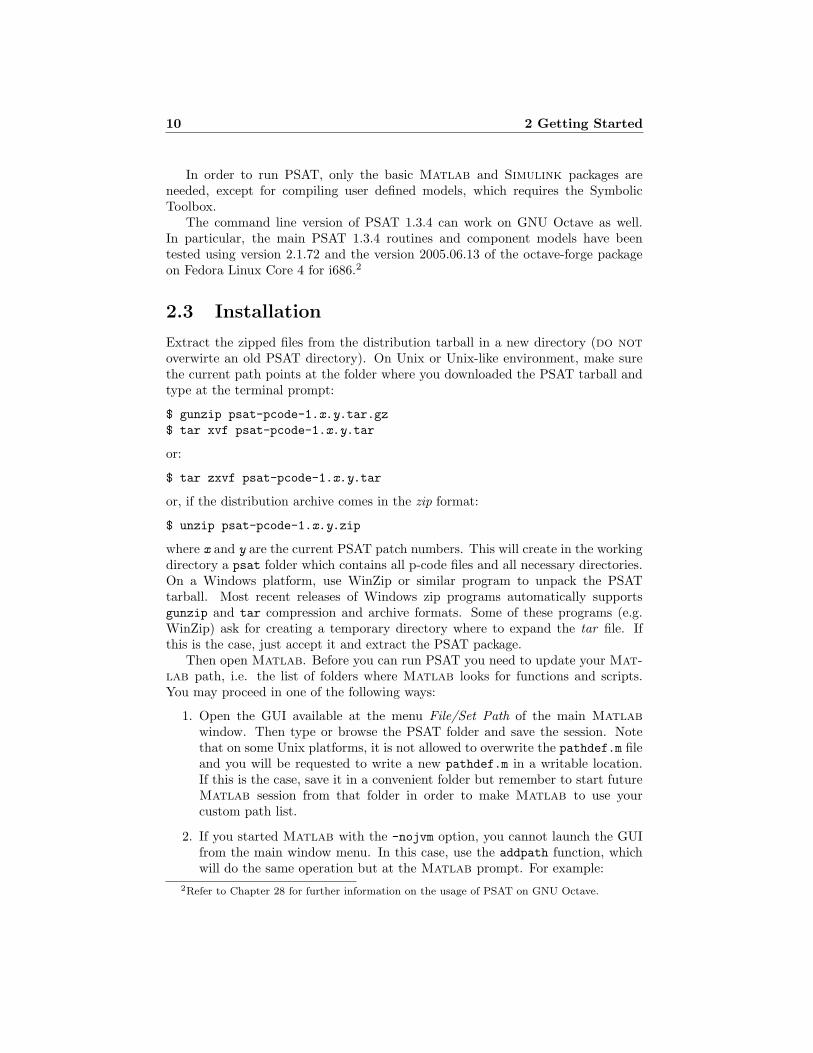
Extract the zipped files from the distribution tarball in a new directory (do notoverwirte an old PSAT directory). On Unix or Unix-like environment, make surethe current path points at the folder where you downloaded the PSAT tarball andtype at the terminal prompt:
$ gunzip psat-pcode-1.x.y.tar.gz
$ tar xvf psat-pcode-1.x.y.tar
or:
$ tar zxvf psat-pcode-1.x.y.tar
or, if the distribution archive comes in the zip format:
$ unzip psat-pcode-1.x.y.zip
where x and y are the current PSAT patch numbers. This will create in the workingdirectory a psat folder which contains all p-code files and all necessary directories.On a Windows platform, use WinZip or similar program to unpack the PSATtarball. Most recent releases of Windows zip programs automatically supportsgunzip and tar compression and archive formats. Some of these programs (e.g.WinZip) ask for creating a temporary directory where to expand the tar file. Ifthis is the case, just accept it and extract the PSAT package.
Then open Matlab. Before you can run PSAT you need to update your Mat-lab path, i.e. the list of folders where Matlab looks for functions and scripts.You may proceed in one of the following ways:
1. Open the GUI available at the menu File/Set Path of the main Matlabwindow. Then type or browse the PSAT folder and save the session. Notethat on some Unix platforms, it is not allowed to overwrite the pathdef.m fileand you will be requested to write a new pathdef.m in a writable location.If this is the case, save it in a convenient folder but remember to start futureMatlab session from that folder in order to make Matlab to use yourcustom path list.
2. If you started Matlab with the -nojvm option, you cannot launch the GUIfrom the main window menu. In this case, use the addpath function, whichwill do the same operation but at the Matlab prompt. For example:
2Refer to Chapter 28 for further information on the usage of PSAT on GNU Octave.

2.4 Launching PSAT 11
>> addpath /home/username/psat
or:
>> addpath ’c:\Document and Settings\username\psat’
For further information, refer to the on-line documentation of the functionaddpath or the Matlab documentation for help.
3. Change the current Matlab working directory to the PSAT folder and launchPSAT from there. This works since PSAT checks the current Matlab pathlist definition when it is launched. If PSAT does not find itself in the list,it will use the addpath function as in the previous point. Using this PSATfeature does not always guarantee that the Matlab path list is properlyupdated and is not recommended. However, this solution is the best choice incase you wish maintaining different PSAT versions in different folders. Justbe sure that in your pathdef.m file there is no PSAT folder. You should alsoupdate the Matlab path or restart Matlab anytime you want to work witha different PSAT version.
4. If you have an older version of PSAT on your computer and this version isworking fine, just expand the PSAT tarball on top of it. Then launch PSATas usual.
Note 1: PSAT will not work properly if the Matlab path does not contain thePSAT folder.
Note 2: PSAT makes use of four internal folders (images, build, themes, andfilters). It is recommended not to change the position and the names of thesefolders. Observe that PSAT can work properly only if the current Matlab folderand the data file folders are writable. Furthermore, also the PSAT folder should bewritable if you want to build and install user defined components.
2.4 Launching PSAT
After setting the PSAT folder in the Matlab path, type from the Matlab prompt:
>> psat
This will create all the structures required by the toolbox, as follows:3
3By default, all variables previously initialized in the workspace are cleared. If this is notdesired, just comment or remove the clear all statement at the beginning of the script filepsat.m.
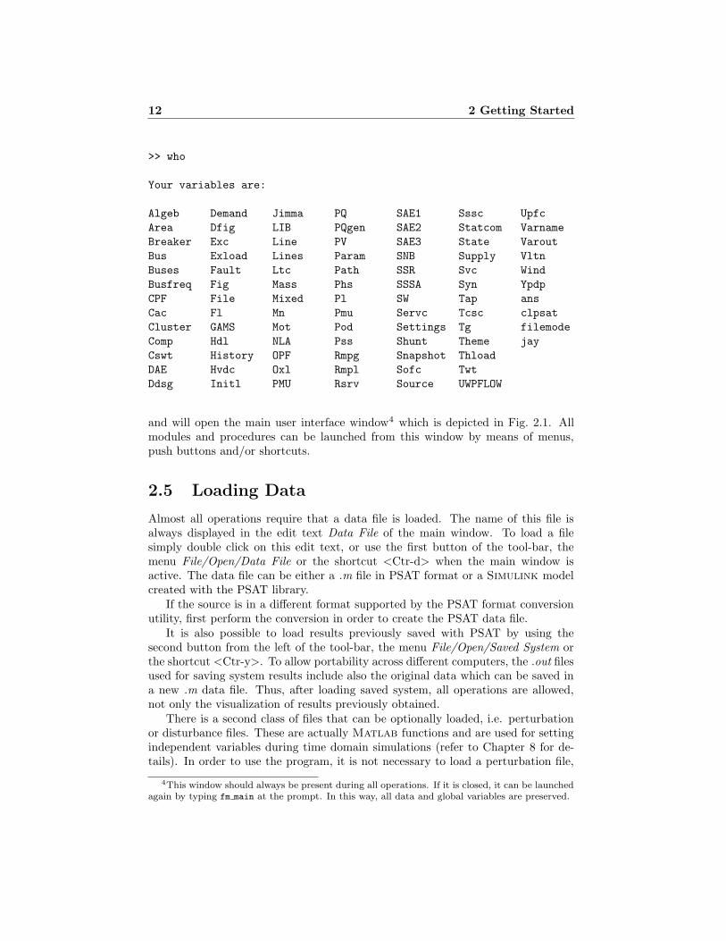
12 2 Getting Started
>> who
Your variables are:
Algeb Demand Jimma PQ SAE1 Sssc Upfc
Area Dfig LIB PQgen SAE2 Statcom Varname
Breaker Exc Line PV SAE3 State Varout
Bus Exload Lines Param SNB Supply Vltn
Buses Fault Ltc Path SSR Svc Wind
Busfreq Fig Mass Phs SSSA Syn Ypdp
CPF File Mixed Pl SW Tap ans
Cac Fl Mn Pmu Servc Tcsc clpsat
Cluster GAMS Mot Pod Settings Tg filemode
Comp Hdl NLA Pss Shunt Theme jay
Cswt History OPF Rmpg Snapshot Thload
DAE Hvdc Oxl Rmpl Sofc Twt
Ddsg Initl PMU Rsrv Source UWPFLOW
and will open the main user interface window4 which is depicted in Fig. 2.1. Allmodules and procedures can be launched from this window by means of menus,push buttons and/or shortcuts.
2.5 Loading Data
Almost all operations require that a data file is loaded. The name of this file isalways displayed in the edit text Data File of the main window. To load a filesimply double click on this edit text, or use the first button of the tool-bar, themenu File/Open/Data File or the shortcut <Ctr-d> when the main window isactive. The data file can be either a .m file in PSAT format or a Simulink modelcreated with the PSAT library.
If the source is in a different format supported by the PSAT format conversionutility, first perform the conversion in order to create the PSAT data file.
It is also possible to load results previously saved with PSAT by using thesecond button from the left of the tool-bar, the menu File/Open/Saved System orthe shortcut <Ctr-y>. To allow portability across different computers, the .out filesused for saving system results include also the original data which can be saved ina new .m data file. Thus, after loading saved system, all operations are allowed,not only the visualization of results previously obtained.
There is a second class of files that can be optionally loaded, i.e. perturbationor disturbance files. These are actually Matlab functions and are used for settingindependent variables during time domain simulations (refer to Chapter 8 for de-tails). In order to use the program, it is not necessary to load a perturbation file,
4This window should always be present during all operations. If it is closed, it can be launchedagain by typing fm main at the prompt. In this way, all data and global variables are preserved.

Figure 2.1: Main graphical user interface of PSAT.
13

14 2 Getting Started
not even for running a time domain simulation.
2.6 Running the Program
Setting a data file does not actually load or update the component structures. Todo this, one has to run the power flow routine, which can be launched in severalways from the main window (e.g. by the shortcut <Ctr-p>). Refer to Chapter 4for details. The last version of the data file is read each time the power flow isperformed. The data are updated also in case of changes in the Simulink modeloriginally loaded. Thus it is not necessary to load again the file every time it ismodified.
After solving the first power flow, the program is ready for further analysis, suchas Continuation Power Flow (Chapter 5), Optimal Power Flow (Chapter 6), SmallSignal Stability Analysis (Chapter 7), Time Domain Simulation (Chapter 8), PMUplacement (Chapter 9), etc. Each of these procedures can be launched from thetool-bar or the menu-bar of the main window.
2.7 Displaying Results
Results can be generally displayed in more than one way, either by means of agraphical user interface in Matlab or as a ascii text file. For example powerflow results, or whatever is the actual solution of the power flow equations of thecurrent system, can be inspected with a GUI (in the main window, look for themenu View/Static Report or use the shortcut <Ctr-v>). Then, the GUI allows tosave the results in a text file. The small signal stability and the PMU placementGUIs have similar behaviors. Other results requiring a graphical output, such ascontinuation power flow results, multi-objective power flow computations or timedomain simulations, can be depicted and saved in .eps files with the plotting utilities(in the main window, look for the menu View/Plotting Utilities or use the shortcut<Ctr-w>). Refer to the chapters where these topics are discussed for details andexamples.
Some computations and several user actions result also in messages stored inthe History structure. These messages/results are displayed one at the time inthe static text banner at the bottom of the main window. By double clicking onthis banner or using the menu Options/History a user interface will display the lastmessages. This utility can be useful for debugging data errors or for checking theperformances of the procedures.5
5All errors displayed in the command history are not actually errors of the program, but aredue to wrong sequence of operations or inconsistencies in the data. On the other hand, errors andwarnings that are displayed on the Matlab prompt are more likely bugs and it would be of greathelp if you could report these errors to me whenever you encounter one.

2.8 Saving Results 15
2.8 Saving Results
At any time the menu File/Save/Current System or the shortcut <Ctr-a> can beinvoked for saving the actual system status in a .mat file. All global structures usedby PSAT are stored in this file which is placed in the folder of the current data fileand has the extension .out. Also the data file itself is saved, to ensure portabilityacross different computers.
Furthermore, all static computations allow to create a report in a text file thatcan be stored and used later. The extensions for these files are as follows:
.txt for reports in plain text;
.xls for reports in Excel;
.tex for reports in LATEX.
The report file name are built as follows:
[data file name] [xx].[ext]
where xx is a progressive number, thus previous report files will not be overwritten.6
All results are placed in the folder of the current data file, thus it is important tobe sure to have the authorization for writing in that folder.
Also the text contained in the command history can be saved, fully or in part,in a [data file name] [xx].log file.
2.9 Settings
The main settings of the system are directly included in the main window an theycan be modified at any time. These settings are the frequency and power bases,starting and ending simulation times, static and dynamic tolerance and maximumnumber of iterations. Other general settings, such as the fixed time step used fortime domain simulations or the setting to force the conversion of PQ loads intoconstant impedances after power flow computations, can be modified in a separatewindows (in the main window, look for the menu Edit/General Settings or usethe shortcut <Ctr-k>). All these settings and data are stored in the Settings
structure which is fully described in Appendix A. The default values for somefields of the Settings structure can be restored by means of the menu Edit/SetDefault. Customized settings can be saved and used as default values for the nextsessions by means of the menu File/Save/Settings.
Computations requiring additional settings have their own structures and GUIsfor modifying structure fields. For example, the continuation power flow analysisrefers to the structure CPF and the optimal power flow analysis to the structureOPF. These structures are described in the chapters dedicated to the correspondingtopics.
6Well, after writing the 99th file, the file with the number 01 is actually overwritten withoutasking for any confirmation.

16 2 Getting Started
A different class of settings is related to the PSAT graphical interface appear-ance, the preferred text viewer for the text outputs and the settings for the com-mand history interface. These features are described in Chapter 26.
2.10 Network Design
The Simulink environment and its graphical features are used in PSAT to createa CAD tool able to design power networks, visualize the topology and change thedata stored in it, without the need of directly dealing with lists of data. However,Simulink has been thought for control diagrams with outputs and inputs variables,and this is not the best way to approach a power system network. Thus, the timedomain routines that come with Simulink and its ability to build control blockdiagrams are not used. PSAT simply reads the data from the Simulink model andwrites down a data file.
The library can be launched from the main window by means of the but-ton with the Simulink icon in the menu-bar, the menu Edit/Network/Edit Net-work/Simulink Library or the shortcut <Ctr-s>. A full description of this libraryan its interactions with the rest of the program is presented in Chapter 21.
2.11 Tools
Several tools are provided with PSAT, e.g. data format conversion functions anduser defined model routines.
The data format conversion routines (see Chapter 24) allow importing data filesfrom other power system software packages. However, observe that in some casesthe conversion cannot be complete since data defined for commercial software havemore features than the ones implemented in PSAT. PSAT static data files can beconverted into the IEEE Common Data Format.
User defined model routines (see Chapter 25) provide a simple way for extendingthe capabilities of PSAT and, hopefully, facilitating contributions. The constructionof a user defined model can be yielded in few steps, as follows:
1. Define parameters and differential and algebraic equations by means of a GUI;
2. Create the Matlab function of the model;7
3. Save the model in a .m file;
4. Install the model in the program, by means of an automatic procedure.
If the component is not needed any longer it can also be “uninstalled” in a similarway. Thus, user defined models can be shared easily by simply providing thecomponent function and the component structure stored in a Matlab script file.However, the routine which compiles model functions is not complete so far, and itis intended only for creating a first draft of the component function.
7The Symbolic Toolbox is required for building the new component function.

2.12 Interfaces 17
Other PSAT tools and utilities, such as the command history, the sparse matrixvisualization GUI, the theme selector, and the text viewer selector are described inChapter 26.
2.12 Interfaces
PSAT provides interfaces to GAMS and UWPFLOW, which highly extend PSATability to perform OPF and CPF analysis respectively.
The General Algebraic Modeling System (GAMS) is a high-level modeling sys-tem for mathematical programming problems. It consists of a language compilerand a variety of integrated high-performance solvers. GAMS is specifically designedfor large and complex scale problems, and allows creating and maintaining mod-els for a wide variety of applications and disciplines [Brooke et al. 1998]. Referto Chapter 29 for a more detailed description of the routine and the GUI whichinterfaces PSAT to GAMS.
UWPFLOW is an open source program for sophisticated continuation powerflow analysis [Canizares and Alvarado 2000]. It consists of a set of C functions andlibraries designed for voltage stability analysis of power systems, including voltagedependent loads, HVDC, FACTS and secondary voltage control. Refer to Chapter30 for a more detailed description of the PSAT-UWPFLOW interface, which allowsexporting PSAT models to UWPFLOW. The interface is currently in an early stage;refer to Section 30.3 for limitations and ToDos.

Chapter 3
News
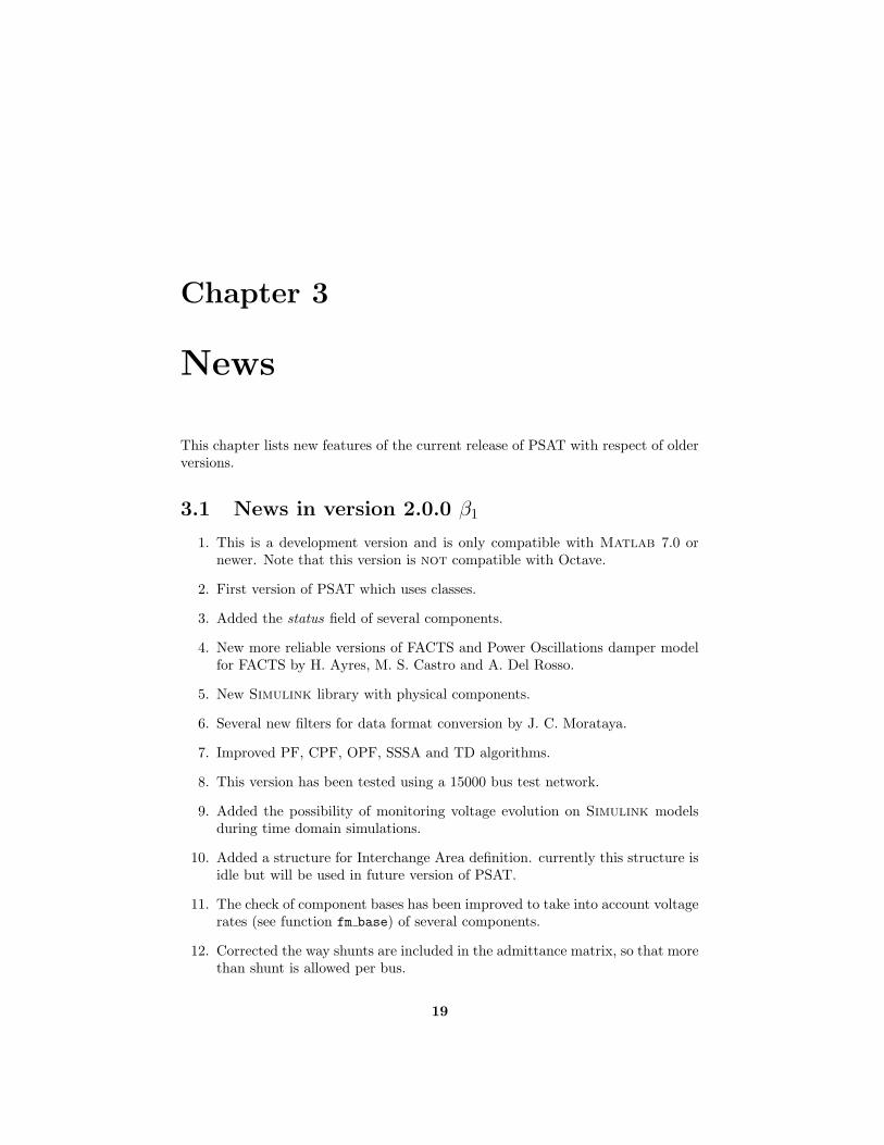
This chapter lists new features of the current release of PSAT with respect of olderversions.
3.1 News in version 2.0.0 β1
1. This is a development version and is only compatible with Matlab 7.0 ornewer. Note that this version is not compatible with Octave.
2. First version of PSAT which uses classes.
3. Added the status field of several components.
4. New more reliable versions of FACTS and Power Oscillations damper modelfor FACTS by H. Ayres, M. S. Castro and A. Del Rosso.
5. New Simulink library with physical components.
6. Several new filters for data format conversion by J. C. Morataya.
7. Improved PF, CPF, OPF, SSSA and TD algorithms.
8. This version has been tested using a 15000 bus test network.
9. Added the possibility of monitoring voltage evolution on Simulink modelsduring time domain simulations.
10. Added a structure for Interchange Area definition. currently this structure isidle but will be used in future version of PSAT.
11. The check of component bases has been improved to take into account voltagerates (see function fm base) of several components.
12. Corrected the way shunts are included in the admittance matrix, so that morethan shunt is allowed per bus.
19

20 3 News
13. Corrected the Jacobian and hessian matrix of apparent power flows in trans-mission line for OPF routine.
14. Changed the logo of PSAT.
3.2 News in version 1.3.4
1. Added unit commintment and multiperiod market clearing models for thePSAT-GAMS interface (see Section 29.5).
2. Added Phasor Measurement Unit (PMU) model (see Section 13.2).
3. Added Jimma’s load model (see Section 14.6).
4. Added mixed load model (see Section 14.7).
5. Added a filter to convert data file in NEPLAN format (see Chapter 24).
6. Added the possibility of exporting plots as MTV plot files and as Matlabscripts. These new features are available from within the GUI for plottingresults.
7. Added a better step control for the continuation power flow analysis. Thestep control can be disabled (menu Options of the CPF GUI), resulting infaster but likely imprecise continuation analysis.
8. Added the option of stopping time domain simulations when the machineangle degree is greater than a given ∆δmax (default value 180).
9. Added the function fm connectivity to detect separation in areas followinga breaker operation during time domain simulation (by courtesy of LaurentLenoir).
10. Added a check during the initialization of synchronous machines to see if aPV or slack generator are connected to the machine bus. In the case thatno PV or slack generator are found a warning message is displayed. Observethe initalization routine does not fail, but the machine is likely not properlyinitialized.
11. Patched the fm sim function. It is now allowed using bus names with carriagereturn characters.
12. Many minor function patches. These are: fm breaker, fm cdf, fm int,fm m2cdf, fm m2wscc, fm ncomp, fm opfm, fm opfsdr, fm pss, fm snb.

3.3 News in version 1.3.3 21
3.3 News in version 1.3.3
1. Minor release with a few bug fixes and a revision of PSAT documentation.
2. The linear recovery load has been renamed exponential recovery load in orderto be consistent with the definition given in [Karlsson and Hill 1994]. Thecorresponding component structure has been renamed Exload.
3.4 News in version 1.3.2
1. First release fully tested on Matlab 7.0 (R14).
2. Added a Physical Model Component Library for Simulink (Only for Mat-lab 6.5.1 or greater).
3. Fixed a bug which did not allow setting fault times t = 0 in dynamic simula-tions.
4. Added the possibilities of exporting time domain simulations as ascii files.
5. Fixed some bugs in the filter for PSS/E 29 data format.
6. Modified the TCSC control system (the first block is now a wash-out filter).
7. Fixed a bug in time domain simulation which produced an error when han-dling snapshots.
8. Corrected several minor bugs in the functions and typos in the documentation(the latter thanks to Marcos Miranda).
9. Successful testing on Matlab 7.0 and octave 2.1.57 & octave-forge 2004-07-07for MAC OS X 10.3.5 (by Randall Smith).
3.5 News in version 1.3.1
1. Added a numeric linear analysis library (contribution by Alberto Del Rosso).
2. Added a new wind turbine model with direct drive synchronous generator(development).
3. Improved models of synchronous generators (which now include a simple q-axis saturation), AVRs and PSSs.
4. Added a filter for PSS/E 29 data format.
5. Added base conversion for flow limits of transmission lines.
6. Corrected a bug in the fm pq function (computation of Jacobian matriceswhen voltage limit control is enabled).

22 3 News
7. Improved continuation power flow routine.
8. Corrected several minor bugs in the functions and typos in the documentation.
9. Fixed a few Octave compatibility issues.
3.6 News in version 1.3.0
1. Added the command line version.
2. Basic compatibility with GNU/Octave (only for command line version).
3. Added wind models, i.e. Weibull distribution and composite wind model.Wind measurement data are supported as well.
4. Added wind turbine models (constant speed wind turbine and doubly fedinduction generator).
5. Bus frequency measurement block.
6. Improved continuation and optimal power flow routines. The continuationpower flow routine allows now using dynamic components (experimental).
7. Improved model of LTC transformers. Discrete tap ratio is now better sup-ported and includes a time delay.
8. Improved PSAT/GAMS interface.
9. Improved the routine for small signal stability analysis. Results and settingsare now contained in the structure SSSA. Output can be exported to Excel,TEX or plain text formats.
10. PMU placement reports can be exported to Excel, TEX or plain text formats.
11. Corrected a few bugs in the PSS function.
3.7 News in version 1.2.2
1. Added the autorun.m function which allows launching any routine withoutsolving the power flow analysis first.
2. Power flow reports can be exported to Excel, TEX or plain text formats.
3. Added filters to convert data files into BPA and Tshingua University formats.
4. Improved model of solid oxide fuel cell. Reactive power output is now includedin the converted model.
5. Overall improvement of the toolbox and its documentation. The stablestrelease so far.

3.8 News in version 1.2.1 23
3.8 News in version 1.2.1
Minor bug-fixing release. Main improvements are in functions psat.m, fm base.m
and fm sim.m.
3.9 News in version 1.2.0
1. First PSAT release which is Matlab version independent.
2. Installation of PSAT folder is now not required, although recommended.
3. Several bug fixes in continuation and optimal power flow routines.
4. Improved fault computation for time domain simulations. These improve-ments remove simulation errors which occurred in previous PSAT versions.
5. Added a new filters in Perl language for data format conversion.
6. Several bugs and typos were removed thanks to Liulin.
3.10 News in version 1.1.0
1. Created the PSAT Forum (http://groups.yahoo.com/group/psatforum).
2. Added PSAT/GAMS interface.
3. Added PSAT/UWPFLOW interface.
4. Added phase shifting transformer model.
5. Added filter for CYMFLOW data format.
6. Corrected some bugs in the filter for MatPower data format.
3.11 News in version 1.0.1
Minor bug-fixing release. Main improvements are in functions fm fault.m and inthe documentation.


Part II
Routines


Chapter 4
Power Flow
This chapter describes routines, settings and graphical user interfaces for power flowcomputations. The standard Newton-Raphson method [Tinney and Hart 1967] andthe Fast Decoupled Power Flow (XB and BX variations [Stott and Alsac 1974, Stott1974, van Amerongen 1989]) are implemented. A power flow with a distributed slackbus model is also included.
4.1 Power Flow Solvers
The power flow problem is formulated as the solution of a nonlinear set of equationsin the form:
x = 0 = f(x, y) (4.1)
0 = g(x, y)
where y (y ∈ R2n), n being the number of buses in the network, are the algebraic
variables, i.e. voltage amplitudes V and phases θ at the network buses, x (x ∈ Rm)
are the state variables, g (g ∈ R2n) are the algebraic equations for the active and
the reactive power balances at each bus1 and f (f ∈ Rm) are the differential equa-
tions. Differential equations are included in (4.1) since PSAT initializes the statevariables of some dynamic components (e.g. induction motors and load tap chang-ers) during power flow computations. Other state variables and control parametersare initialized after solving the power flow solution (e.g. synchronous machines andregulators). Refer to Section 4.1.4 for the complete list of components that areincluded in or initialized after the power flow solution.
4.1.1 Newton-Raphson Method
Newton-Raphson algorithms for solving the power flow problem are described inmany books and papers (e.g. [Tinney and Hart 1967]). At each iteration, the
1The algebraic equations g are internally stored in two vectors, gP (gP ∈ Rn) and gQ (gQ ∈ R
n)which represent the active and reactive power balances respectively.
27

28 4 Power Flow
Jacobian matrix of (4.1) is updated and the following linear problem is solved:
[∆xi
∆yi
]= −
[F i
x −F iy
Gix J i
LFV
]−1 [f i
gi
](4.2)
[xi+1
yi+1
]=
[xi
yi
]+
[∆xi
∆yi
]
where Fx = ∇xf , Fy = ∇yf , Gx = ∇xg and JLFV = ∇yg. If the variableincrements ∆x and ∆y are lower than a given tolerance ε or the number of iterationis greater than a given limit (i > imax) the routine stops. The power flow Jacobianmatrix JLFV is always built such that JLFV ∈ R
2n×2n as follows:
- The column of the derivatives with respect to the reference angle is set tozero;
- The columns of the derivatives with respect to generator voltages are set tozero;
- The row of the derivatives of the slack bus active power balance gPslackis set
to zero;
- The rows of the derivatives of generator reactive power balances gQ are setto zero;
- Diagonal elements at the intersections of the columns and the rows describedabove are set to one;
- The elements of the vector g associated with the generator reactive powersand the slack bus active power are set to zero.
These assumptions are equivalent to the trivial equations:
θslack = θslack0(4.3)
VG = VG0
where θslack is the voltage phase of the reference bus and VG the vector of generatorvoltages. Although forcing the dimensions of JLFV to be always maximum (i.e. 2n),this formulation is not computationally expensive, since the properties of Matlabsparse matrices are used.
4.1.2 Fast Decoupled Power Flow
The Fast Decoupled Power Flow (FDPF) was originally proposed in [Stott andAlsac 1974] and has been further developed and generalized in several variations.PSAT uses the XB and BX methods presented in [van Amerongen 1989].
The power flow Jacobian matrix JLFV can be decomposed in four sub-matrices:
JLFV =
[JPθ JPV
JQθ JQV
](4.4)

4.1 Power Flow Solvers 29
where JPθ = ∇θgP , JPV = ∇V gP , JQθ = ∇θgQ, and JPθ = ∇V gQ. The basicassumptions of FDPF methods are:
JPV = 0 (4.5)
JQθ = 0
JPθ ≈ B′
JQV ≈ B′′
where B′ and B′′ can be thought as admittance matrices with the following sim-plifications:
1. Line charging, shunts and transformer tap ratios are neglected when comput-ing B′;
2. Phase shifters are neglected and line charging and shunts are doubled whencomputing B′′.
The XB and BX variations differ only in further simplifications of the B ′ and B′′
matrices respectively, as follows:
XB: line resistances are neglected when computing B ′;
BX: line resistances are neglected when computing B ′′.
Thus the FDPF consists in turn of solving two systems at each iteration, as follows:
∆gi′
P /Vi′ = B′∆θi′ (4.6)
∆gi′′
Q /Vi′′ = B′′∆V i′′
where ∆gP and ∆gQ are the active and reactive power flow equation mismatches.The solution of the active equations is used as input to the reactive ones, as thisreduces the number of iterations.
PSAT allows using FDPF methods for system which contain only PV generators,PQ loads and one slack bus. If other components are present in the network, thestandard Newton-Raphson routine is used.
4.1.3 Distributed Slack Bus Model
The distributed slack bus model is based on a generalized power center concept andconsists in distributing losses among all generators [Barcelo and Lemmon 1988].This is practically obtained by including in (4.1) a variable kG and rewriting thesystem active power balance as follows:
nG∑
i
(1 + kGγi)PGi−
nP∑
i
PLi− Plosses = 0 (4.7)
Equations (4.2) are modified by adding to the Jacobian matrix JLFV the row of thederivatives of the slack bus active power balance and a column for the derivatives

30 4 Power Flow
of differential and algebraic equations with respect to kG. The additional param-eter γ is also included in order to allow tuning the weight of the participation ofeach generator to the losses. (In the single slack bus model, γ = 0 for all gener-ators but one.) When the distributed slack bus flag is active, FDPF methods areautomatically disabled.
4.1.4 Initialization of State Variables
Dynamic components and non-conventional loads can be included in or initializedafter the power flow solution. The following components are included in the powerflow equation set:
Hvdc Lines Ltc Mn Mot PQ PV
Phs Pl SAE1 SAE2 SAE3 SW Tap
whereas the following ones are initialized after solving the power flow problem:
Busfreq Cac Cluster Cswt Ddsg Dfig Exc
Fl Exload Mass Mn Oxl Pl Pod
Pss SSR Sofc Statcom Sssc Svc Syn
Tcsc Tg Thload Upfc Wind
Voltage dependent and ZIP loads (Mn and Pl) appears in both lists since theirinclusion in the power flow computation is an available option. Refer to the specificdescriptions of each component for details.
4.2 Settings
General settings for power flow computations, i.e. power and frequency rates ofthe system, convergence tolerance and maximum number of iterations used forthe Newton-Raphson/FDPF techniques can be set in the main window. Otherparameters can be customized in the GUI for general settings (menu Edit/GeneralSettings or shortcut <Ctr-k> in the main window), which is depicted in Fig. 4.1.The following options are available for power flow analysis:
Power Flow Solver: these are the Newton-Raphson (NR) method, the fast decou-pled XB and BX methods. Observe that only the NR method is available ifthe distributed slack bus option is enabled or if there are dynamic componentincluded in the power flow analysis.
Use Distributed Slack Bus: this option allows using distributed slack bus model,i.e. all PV buses contributes to system losses, not only the reference anglebus. this option is disabled if there are dynamic component included in thepower flow analysis.

4.3 Example 31
Check Component Bases: enable checking component power and voltage ratings.The check of the consistency of component ratings is made by the functionfm base.m. Only a reduced number of component are checked. Refer to thecode for details.
Discard Dynamic Comp.: if this option is enabled, dynamic components initializedafter the power flow are discarded. Observe that dynamic components thatare included in the power flow analysis are retained.
Check PV Reactive Limits: this option forces checking reactive power limits of PVbuses. If a limit is reached, the PV bus is converted into a PQ bus. Novoltage recovery is taken into account. More precise results can be obtainedusing the continuation power flow analysis.
Show Iteration Status: display the absolute minimum convergence error in the mainwindow during power flow analysis.
Show Power Flow Results: open the static report GUI and display power flow re-sults when power flow analysis has completed.
Power flow settings are stored in the structure Settings, which contains alsogeneral settings and parameters for time domain simulations. This structure is fullydescribed in Appendix A.
4.3 Example
Figure 4.2 depicts the GUI for power flow results. Data refer to a 9-bus test systempresented and discussed in [Sauer and Pai 1998]. The GUI reports the bus namesand their correspondent voltages and total power injections. Voltage profiles canbe plotted using the buttons on top of the lists for voltage magnitudes and angles.Angles can be expressed either in radiants or degrees. If the loaded system presentsstate and control variables, these are reported in the GUI as well. Power flowresults can be saved using the Report button. A log file will be created using theselected format (plain text, LATEX, Excel) and displayed with the selected viewer(see Section 26.4 for details). For example, the plain text power flow solution forthe WSCC 9-bus test system is as follows:
POWER FLOW REPORT
P S A T 1.3.4
Author: Federico Milano, (c) 2002-2005
e-mail: [email protected]
website: http://thunderbox.uwaterloo.ca/~fmilano
File: ~/psat/tests/d_009.mdl
Date: 26-Oct-2003 12:53:43
NETWORK STATISTICS

Figure 4.1: GUI for general settings.
32
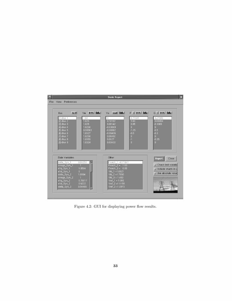
Figure 4.2: GUI for displaying power flow results.
33

34 4 Power Flow
Bus: 9
Lines: 6
Transformers: 3
Generators: 3
Loads: 3
SOLUTION STATISTICS
Number of Iterations: 4
Maximum P mismatch [p.u.] 0
Maximum Q mismatch [p.u.] 0
Power rate [MVA] 100
POWER FLOW RESULTS
Bus V phase P gen Q gen P load Q load
[p.u.] [rad] [p.u.] [p.u.] [p.u.] [p.u.]
Bus 1 1.04 0 0.71641 0.27046 0 0
Bus 2 1.025 0.16197 1.63 0.06654 0 0
Bus 3 1.025 0.08142 0.85 -0.1086 0 0
Bus 4 1.0258 -0.03869 0 0 0 0
Bus 5 0.99563 -0.06962 0 0 1.25 0.5
Bus 6 1.0127 -0.06436 0 0 0.9 0.3
Bus 7 1.0258 0.06492 0 0 0 0
Bus 8 1.0159 0.0127 0 0 1 0.35
Bus 9 1.0324 0.03433 0 0 0 0
STATE VECTOR
delta_Syn_1 1.0664
omega_Syn_1 1
e1q_Syn_1 0.78817
e1d_Syn_1 0.6222
delta_Syn_2 0.94486
omega_Syn_2 1
e1q_Syn_2 0.76786
e1d_Syn_2 0.62424
delta_Syn_3 0.06258
omega_Syn_3 1
e1q_Syn_3 1.0564
e1d_Syn_3 0
vm_Exc_1 1.025
vr1_Exc_1 1.446
vr2_Exc_1 -0.25254
efd_Exc_1 1.403
vm_Exc_2 1.025
vr1_Exc_2 1.8951
vr2_Exc_2 -0.32208
efd_Exc_2 1.7893
vm_Exc_3 1.04
vr1_Exc_3 1.1006
vr2_Exc_3 -0.19479
efd_Exc_3 1.0822
MECHANICAL POWERS & FIELD VOLTAGES
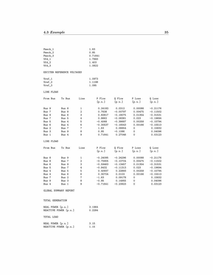
4.3 Example 35
Pmech_1 1.63
Pmech_2 0.85
Pmech_3 0.71641
Vfd_1 1.7893
Vfd_2 1.403
Vfd_3 1.0822
EXCITER REFERENCE VOLTAGES
Vref_1 1.0973
Vref_2 1.1198
Vref_3 1.095
LINE FLOWS
From Bus To Bus Line P Flow Q Flow P Loss Q Loss
[p.u.] [p.u.] [p.u.] [p.u.]
Bus 9 Bus 8 1 0.24183 0.0312 0.00088 -0.21176
Bus 7 Bus 8 2 0.7638 -0.00797 0.00475 -0.11502
Bus 9 Bus 6 3 0.60817 -0.18075 0.01354 -0.31531
Bus 7 Bus 5 4 0.8662 -0.08381 0.023 -0.19694
Bus 5 Bus 4 5 -0.4068 -0.38687 0.00258 -0.15794
Bus 6 Bus 4 6 -0.30537 -0.16543 0.00166 -0.15513
Bus 2 Bus 7 7 1.63 0.06654 0 0.15832
Bus 3 Bus 9 8 0.85 -0.1086 0 0.04096
Bus 1 Bus 4 9 0.71641 0.27046 0 0.03123
LINE FLOWS
From Bus To Bus Line P Flow Q Flow P Loss Q Loss
[p.u.] [p.u.] [p.u.] [p.u.]
Bus 8 Bus 9 1 -0.24095 -0.24296 0.00088 -0.21176
Bus 8 Bus 7 2 -0.75905 -0.10704 0.00475 -0.11502
Bus 6 Bus 9 3 -0.59463 -0.13457 0.01354 -0.31531
Bus 5 Bus 7 4 -0.8432 -0.11313 0.023 -0.19694
Bus 4 Bus 5 5 0.40937 0.22893 0.00258 -0.15794
Bus 4 Bus 6 6 0.30704 0.0103 0.00166 -0.15513
Bus 7 Bus 2 7 -1.63 0.09178 0 0.15832
Bus 9 Bus 3 8 -0.85 0.14955 0 0.04096
Bus 4 Bus 1 9 -0.71641 -0.23923 0 0.03123
GLOBAL SUMMARY REPORT
TOTAL GENERATION
REAL POWER [p.u.] 3.1964
REACTIVE POWER [p.u.] 0.2284
TOTAL LOAD
REAL POWER [p.u.] 3.15
REACTIVE POWER [p.u.] 1.15

36 4 Power Flow
TOTAL SHUNT
REAL POWER [p.u.] 0
REACTIVE POWER (IND) [p.u.] 0
REACTIVE POWER (CAP) [p.u.] 0
TOTAL LOSSES
REAL POWER [p.u.] 0.04641
REACTIVE POWER [p.u.] -0.9216
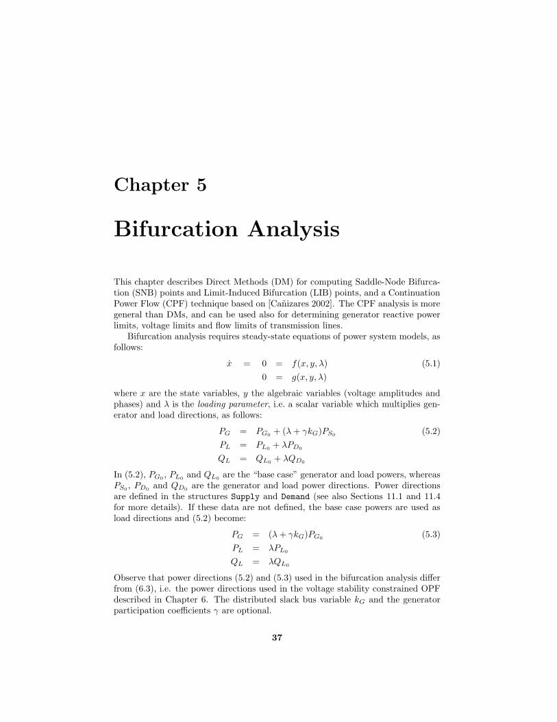
Chapter 5
Bifurcation Analysis
This chapter describes Direct Methods (DM) for computing Saddle-Node Bifurca-tion (SNB) points and Limit-Induced Bifurcation (LIB) points, and a ContinuationPower Flow (CPF) technique based on [Canizares 2002]. The CPF analysis is moregeneral than DMs, and can be used also for determining generator reactive powerlimits, voltage limits and flow limits of transmission lines.
Bifurcation analysis requires steady-state equations of power system models, asfollows:
x = 0 = f(x, y, λ) (5.1)
0 = g(x, y, λ)
where x are the state variables, y the algebraic variables (voltage amplitudes andphases) and λ is the loading parameter, i.e. a scalar variable which multiplies gen-erator and load directions, as follows:
PG = PG0+ (λ+ γkG)PS0
(5.2)
PL = PL0+ λPD0
QL = QL0+ λQD0
In (5.2), PG0, PL0
and QL0are the “base case” generator and load powers, whereas
PS0, PD0
and QD0are the generator and load power directions. Power directions
are defined in the structures Supply and Demand (see also Sections 11.1 and 11.4for more details). If these data are not defined, the base case powers are used asload directions and (5.2) become:
PG = (λ+ γkG)PG0(5.3)
PL = λPL0
QL = λQL0
Observe that power directions (5.2) and (5.3) used in the bifurcation analysis differfrom (6.3), i.e. the power directions used in the voltage stability constrained OPFdescribed in Chapter 6. The distributed slack bus variable kG and the generatorparticipation coefficients γ are optional.
37

38 5 Bifurcation Analysis
5.1 Direct Methods
Direct Methods which are implemented in PSAT allow to compute the value of theloading parameter λ for at Saddle-Node Bifurcation points and at Limit-InducedBifurcation points.
In PSAT, Direct Methods can perform only “static” bifurcation analysis, i.e.make use of static power flow models (see Chapter 10). Thus, (5.1) reduce to thealgebraic set g. Before running any direct method routine, the power flow analysishas to be run first to initialize the algebraic variables.
5.1.1 Saddle-Node Bifurcation
The conditions for a SNB point are as follows:
g(y, λ) = 0 (5.4)
∇yg(y, λ)v = 0
|v| = 1
or
g(y, λ) = 0 (5.5)
∇yg(y, λ)Tw = 0
|w| = 1
where v and w are the right and the left eigenvectors respectively, and the Euclideannorm is used for the | · | operator. The Euclidean norm reduces the sparsity of theJacobian matrix, but allows to avoid re-factorizations (as happens in the case of∞-norm) and is numerically more stable than the 1-norm. The solution for (5.4)and (5.5) are obtained by means of a Newton-Raphson technique , and the completeJacobian matrix is computed explicitly:
∇yg 0 ∇λg∇yygv ∇yg 0
0 ∇v(|v|) 0
(5.6)
Since the Hessian matrix ∇yyg is computed analytically, this method can be appliedonly to a limited number of components, namely (SW, PV , PQ and Line), whichanyway are the standard models used in power flow analysis. The SNB routinesearches a “good” initial guess for the eigenvectors v and w. However the best wayto initialize the SNB routine is to run first a CPF analysis.
Figure 5.1 depicts the GUI for SNB settings. A complete description of SNBsettings is reported in Appendix A.
5.1.2 Limit Induced Bifurcation
Limit Induced Bifurcation points are defined as the solution of the following system:
0 = g(y, λ) (5.7)
0 = ρ(y)
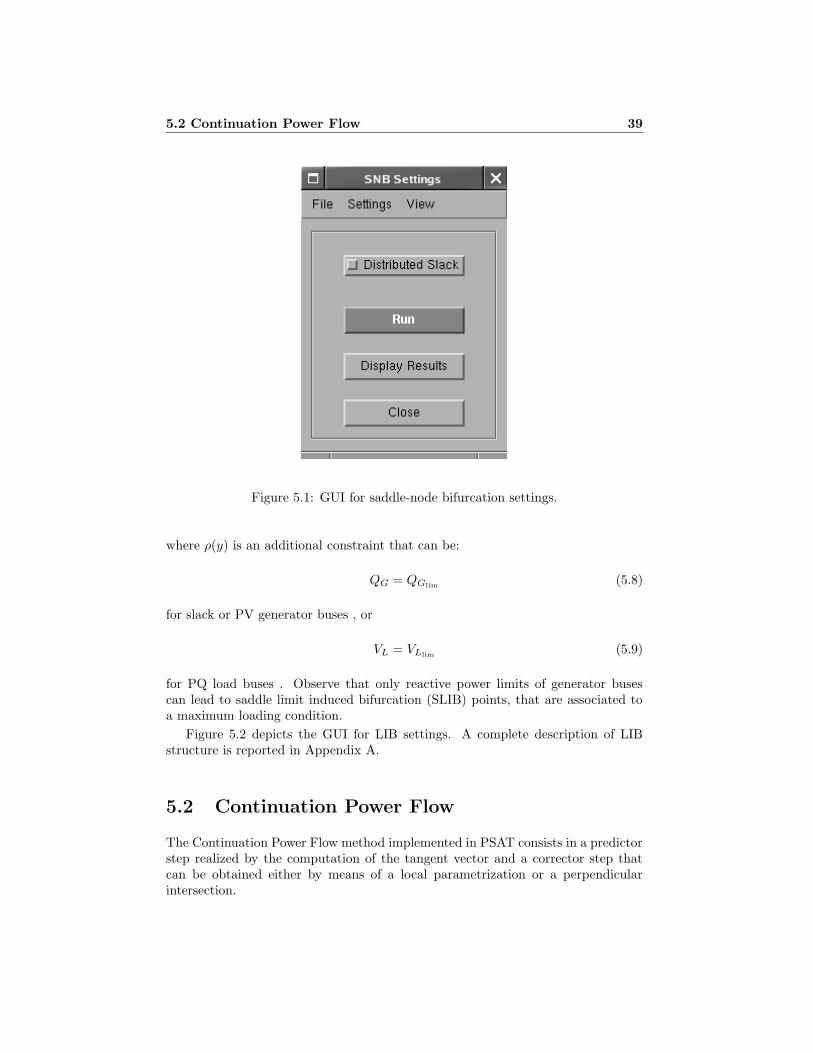
5.2 Continuation Power Flow 39
Figure 5.1: GUI for saddle-node bifurcation settings.
where ρ(y) is an additional constraint that can be:
QG = QGlim(5.8)
for slack or PV generator buses , or
VL = VLlim(5.9)
for PQ load buses . Observe that only reactive power limits of generator busescan lead to saddle limit induced bifurcation (SLIB) points, that are associated toa maximum loading condition.
Figure 5.2 depicts the GUI for LIB settings. A complete description of LIBstructure is reported in Appendix A.
5.2 Continuation Power Flow
The Continuation Power Flow method implemented in PSAT consists in a predictorstep realized by the computation of the tangent vector and a corrector step thatcan be obtained either by means of a local parametrization or a perpendicularintersection.

Figure 5.2: GUI for limit-induced bifurcation settings.
40
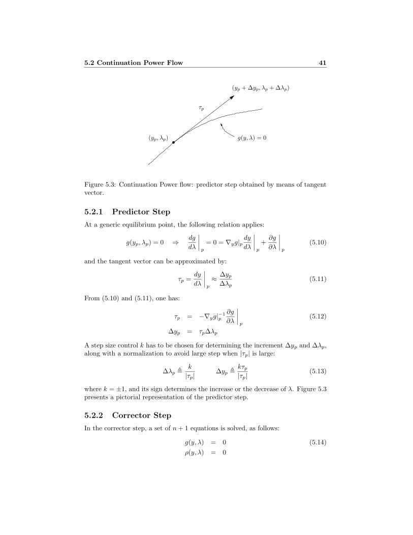
5.2 Continuation Power Flow 41
PSfrag replacements
τp
(yp, λp)
(yp + ∆yp, λp + ∆λp)
g(y, λ) = 0
Figure 5.3: Continuation Power flow: predictor step obtained by means of tangentvector.
5.2.1 Predictor Step
At a generic equilibrium point, the following relation applies:
g(yp, λp) = 0 ⇒ dg
dλ
p
= 0 = ∇yg|pdy
dλ
p
+∂g
∂λ
p
(5.10)
and the tangent vector can be approximated by:
τp =dy
dλ
p
≈ ∆yp
∆λp(5.11)
From (5.10) and (5.11), one has:
τp = −∇yg|−1p
∂g
∂λ
p
(5.12)
∆yp = τp∆λp
A step size control k has to be chosen for determining the increment ∆yp and ∆λp,along with a normalization to avoid large step when |τp| is large:
∆λp ,k
|τp|∆yp ,
kτp|τp|
(5.13)
where k = ±1, and its sign determines the increase or the decrease of λ. Figure 5.3presents a pictorial representation of the predictor step.
5.2.2 Corrector Step
In the corrector step, a set of n+ 1 equations is solved, as follows:
g(y, λ) = 0 (5.14)
ρ(y, λ) = 0
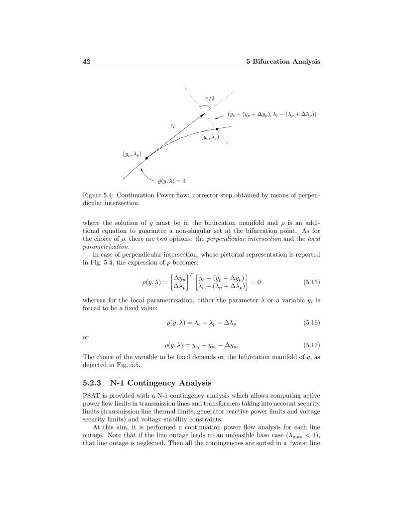
42 5 Bifurcation Analysis
PSfrag replacements
τp
(yp, λp)
(yc, λc)
(yc − (yp + ∆yp), λc − (λp + ∆λp))
g(y, λ) = 0
π/2
Figure 5.4: Continuation Power flow: corrector step obtained by means of perpen-dicular intersection.
where the solution of g must be in the bifurcation manifold and ρ is an addi-tional equation to guarantee a non-singular set at the bifurcation point. As forthe choice of ρ, there are two options: the perpendicular intersection and the localparametrization.
In case of perpendicular intersection, whose pictorial representation is reportedin Fig. 5.4, the expression of ρ becomes:
ρ(y, λ) =
[∆yp
∆λp
]T [yc − (yp + ∆yp)λc − (λp + ∆λp)
]= 0 (5.15)
whereas for the local parametrization, either the parameter λ or a variable yi isforced to be a fixed value:
ρ(y, λ) = λc − λp − ∆λp (5.16)
orρ(y, λ) = yci
− ypi− ∆ypi
(5.17)
The choice of the variable to be fixed depends on the bifurcation manifold of g, asdepicted in Fig. 5.5.
5.2.3 N-1 Contingency Analysis
PSAT is provided with a N-1 contingency analysis which allows computing activepower flow limits in transmission lines and transformers taking into account securitylimits (transmission line thermal limits, generator reactive power limits and voltagesecurity limits) and voltage stability constraints.
At this aim, it is performed a continuation power flow analysis for each lineoutage. Note that if the line outage leads to an unfeasible base case (λmax < 1),that line outage is neglected. Then all the contingencies are sorted in a “worst line
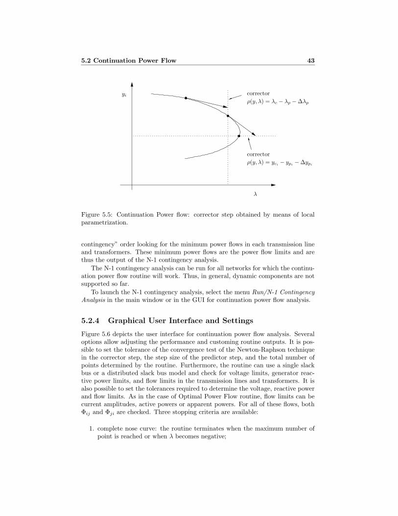
5.2 Continuation Power Flow 43
PSfrag replacements
corrector
corrector
yi
λ
ρ(y, λ) = λc − λp − ∆λp
ρ(y, λ) = yci− ypi
− ∆ypi
Figure 5.5: Continuation Power flow: corrector step obtained by means of localparametrization.
contingency” order looking for the minimum power flows in each transmission lineand transformers. These minimum power flows are the power flow limits and arethus the output of the N-1 contingency analysis.
The N-1 contingency analysis can be run for all networks for which the continu-ation power flow routine will work. Thus, in general, dynamic components are notsupported so far.
To launch the N-1 contingency analysis, select the menu Run/N-1 ContingencyAnalysis in the main window or in the GUI for continuation power flow analysis.
5.2.4 Graphical User Interface and Settings
Figure 5.6 depicts the user interface for continuation power flow analysis. Severaloptions allow adjusting the performance and customing routine outputs. It is pos-sible to set the tolerance of the convergence test of the Newton-Raphson techniquein the corrector step, the step size of the predictor step, and the total number ofpoints determined by the routine. Furthermore, the routine can use a single slackbus or a distributed slack bus model and check for voltage limits, generator reac-tive power limits, and flow limits in the transmission lines and transformers. It isalso possible to set the tolerances required to determine the voltage, reactive powerand flow limits. As in the case of Optimal Power Flow routine, flow limits can becurrent amplitudes, active powers or apparent powers. For all of these flows, bothΦij and Φji are checked. Three stopping criteria are available:
1. complete nose curve: the routine terminates when the maximum number ofpoint is reached or when λ becomes negative;
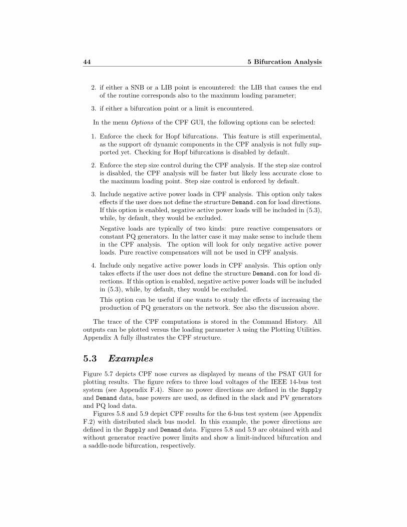
44 5 Bifurcation Analysis
2. if either a SNB or a LIB point is encountered: the LIB that causes the endof the routine corresponds also to the maximum loading parameter;
3. if either a bifurcation point or a limit is encountered.
In the menu Options of the CPF GUI, the following options can be selected:
1. Enforce the check for Hopf bifurcations. This feature is still experimental,as the support ofr dynamic components in the CPF analysis is not fully sup-ported yet. Checking for Hopf bifurcations is disabled by default.
2. Enforce the step size control during the CPF analysis. If the step size controlis disabled, the CPF analysis will be faster but likely less accurate close tothe maximum loading point. Step size control is enforced by default.
3. Include negative active power loads in CPF analysis. This option only takeseffects if the user does not define the structure Demand.con for load directions.If this option is enabled, negative active power loads will be included in (5.3),while, by default, they would be excluded.
Negative loads are typically of two kinds: pure reactive compensators orconstant PQ generators. In the latter case it may make sense to include themin the CPF analysis. The option will look for only negative active powerloads. Pure reactive compensators will not be used in CPF analysis.
4. Include only negative active power loads in CPF analysis. This option onlytakes effects if the user does not define the structure Demand.con for load di-rections. If this option is enabled, negative active power loads will be includedin (5.3), while, by default, they would be excluded.
This option can be useful if one wants to study the effects of increasing theproduction of PQ generators on the network. See also the discussion above.
The trace of the CPF computations is stored in the Command History. Alloutputs can be plotted versus the loading parameter λ using the Plotting Utilities.Appendix A fully illustrates the CPF structure.
5.3 Examples
Figure 5.7 depicts CPF nose curves as displayed by means of the PSAT GUI forplotting results. The figure refers to three load voltages of the IEEE 14-bus testsystem (see Appendix F.4). Since no power directions are defined in the Supply
and Demand data, base powers are used, as defined in the slack and PV generatorsand PQ load data.
Figures 5.8 and 5.9 depict CPF results for the 6-bus test system (see AppendixF.2) with distributed slack bus model. In this example, the power directions aredefined in the Supply and Demand data. Figures 5.8 and 5.9 are obtained with andwithout generator reactive power limits and show a limit-induced bifurcation anda saddle-node bifurcation, respectively.
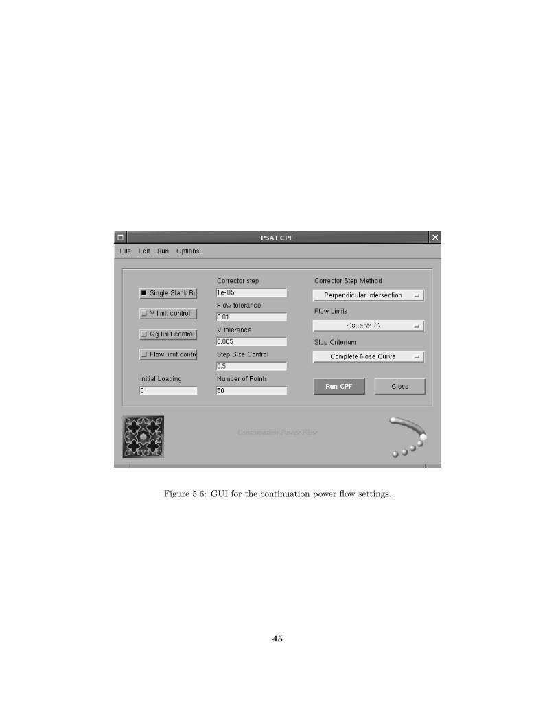
Figure 5.6: GUI for the continuation power flow settings.
45
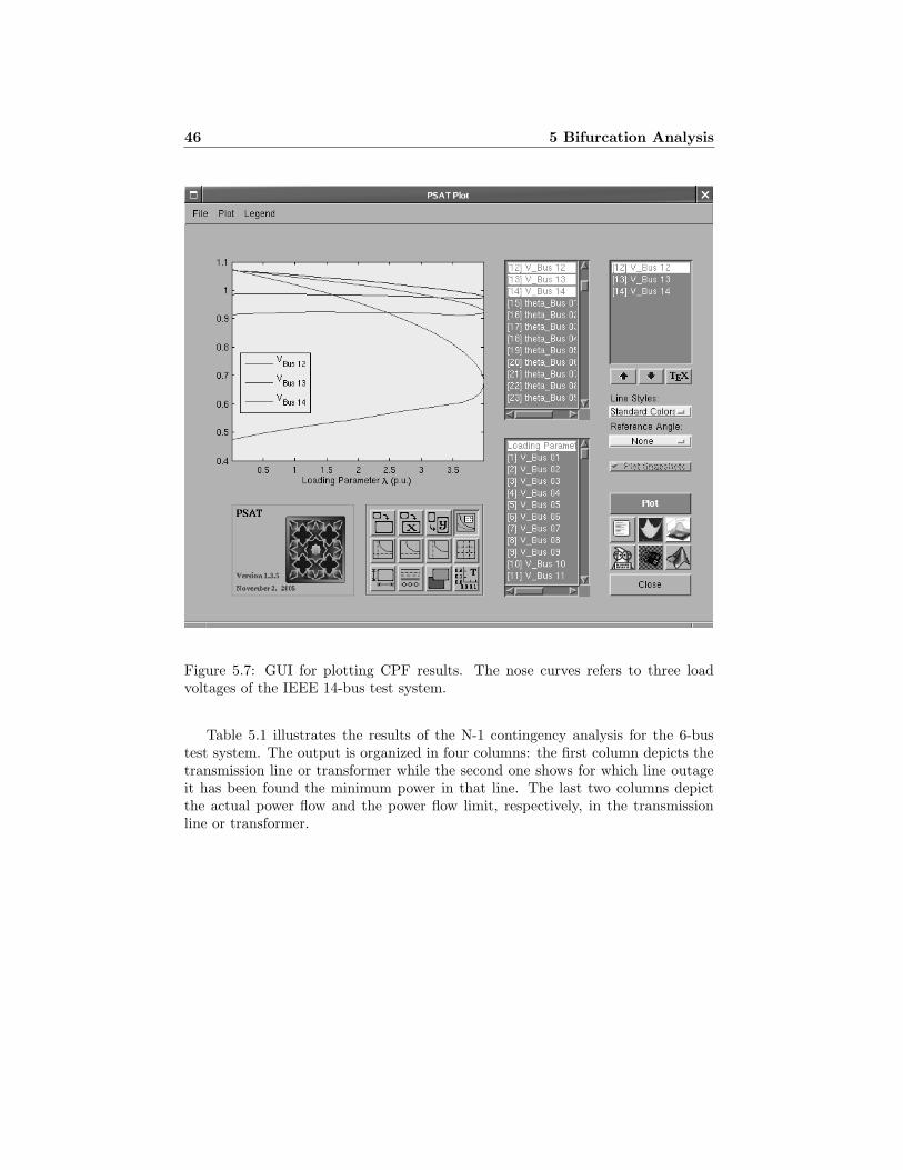
46 5 Bifurcation Analysis
Figure 5.7: GUI for plotting CPF results. The nose curves refers to three loadvoltages of the IEEE 14-bus test system.
Table 5.1 illustrates the results of the N-1 contingency analysis for the 6-bustest system. The output is organized in four columns: the first column depicts thetransmission line or transformer while the second one shows for which line outageit has been found the minimum power in that line. The last two columns depictthe actual power flow and the power flow limit, respectively, in the transmissionline or transformer.

0 0.5 1 1.5 2 2.5 3 3.5 4 4.5 5 5.50.2
0.3
0.4
0.5
0.6
0.7
0.8
0.9
1
1.1
PSfrag replacements
Vol
tage
s[p
.u.]
Loading Parameter λ
VBus 1VBus 2VBus 3VBus 4VBus 5VBus 6
Figure 5.8: Nose curves for the 6-bus test system with generator reactive powerlimits. The maximum loading condition is due to a saddle limit-induced bifurcation.
47
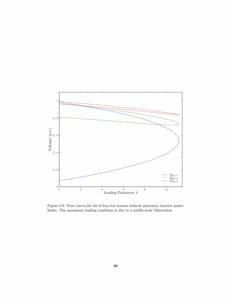
0 2 4 6 8 100
0.2
0.4
0.6
0.8
1
PSfrag replacements
Vol
tage
s[p
.u.]
Loading Parameter λ
VBus 4VBus 5VBus 6
Figure 5.9: Nose curves for the 6-bus test system without generator reactive powerlimits. The maximum loading condition is due to a saddle-node bifurcation.
48
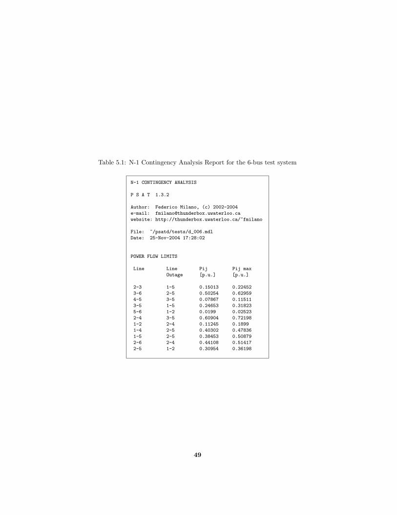
Table 5.1: N-1 Contingency Analysis Report for the 6-bus test system
N-1 CONTINGENCY ANALYSIS
P S A T 1.3.2
Author: Federico Milano, (c) 2002-2004
e-mail: [email protected]
website: http://thunderbox.uwaterloo.ca/~fmilano
File: ~/psatd/tests/d_006.mdl
Date: 25-Nov-2004 17:28:02
POWER FLOW LIMITS
Line Line Pij Pij max
Outage [p.u.] [p.u.]
2-3 1-5 0.15013 0.22452
3-6 2-5 0.50254 0.62959
4-5 3-5 0.07867 0.11511
3-5 1-5 0.24653 0.31823
5-6 1-2 0.0199 0.02523
2-4 3-5 0.60904 0.72198
1-2 2-4 0.11245 0.1899
1-4 2-5 0.40302 0.47836
1-5 2-5 0.38453 0.50879
2-6 2-4 0.44108 0.51417
2-5 1-2 0.30954 0.36198
49


Chapter 6
Optimal Power Flow
This chapter describes the Optimal Power Flow (OPF) problem and its implemen-tation in PSAT. The Interior Point Method (IPM) is used for solving the nonlinearset of equations of the OPF problem as described in [Torres and Quintana 1999].A discussion of diverse objective functions and OPF models used in the program ispresented along with a detailed description of the structures and the data neededto solve the OPF. Finally, a simple 6-bus system example is presented and thegraphical user interface and text outputs are described.
6.1 Interior Point Method
In [Huneault and Galiana 1991], several strategies were proposed for an OPF withactive power dispatching and voltage security using an IPM that proved to berobust, especially in large networks, as the number of iterations increase slightlywith the number of constraints and network size. Most implementations of IPMfor solving market problems, accounting somewhat for system security, use a linearprogramming technique [Stott et al. 1979, Monmoh et al. 1994, Alsac et al. 1990].
In [Quintana and Torres 1996] and [Torres and Quintana 1999], the authorspresent a comprehensive investigation of the use of IPM for non-linear problems,and describe the application of Newton direction method and Merhotra’s predictor-corrector to the OPF. The latter highly reduces the number of iterations to obtainthe final solution. Both methods which were described in [Torres and Quintana1999] are implemented in the IPM-NLP problem.
Non-linear optimization techniques have also been shown to be adequate for ad-dressing a variety of voltage stability issues, such as the maximization of the loadingparameter in voltage collapse studies, as discussed in [Irisarri et al. 1997], [Canizares1998], [Canizares et al. 2000] and [Canizares, Rosehart, Berizzi and Bovo 2001].In [Madrigal and Quintana 1998] and [Madrigal 2000], non-linear IPM techniquesare applied to the solution of diverse OPF market problems. The OPF routinesimplemented in the program also uses the techniques proposed in [Canizares, Chenand Rosehart 2001] and [Milano et al. 2003], where the authors proposed diverse
51
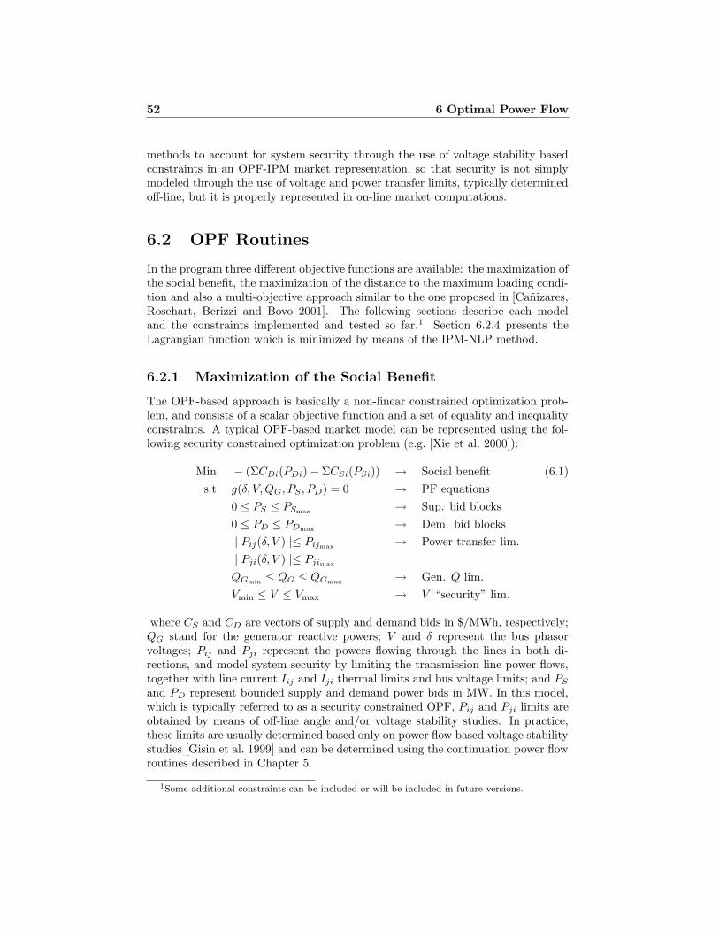
52 6 Optimal Power Flow
methods to account for system security through the use of voltage stability basedconstraints in an OPF-IPM market representation, so that security is not simplymodeled through the use of voltage and power transfer limits, typically determinedoff-line, but it is properly represented in on-line market computations.
6.2 OPF Routines
In the program three different objective functions are available: the maximization ofthe social benefit, the maximization of the distance to the maximum loading condi-tion and also a multi-objective approach similar to the one proposed in [Canizares,Rosehart, Berizzi and Bovo 2001]. The following sections describe each modeland the constraints implemented and tested so far.1 Section 6.2.4 presents theLagrangian function which is minimized by means of the IPM-NLP method.
6.2.1 Maximization of the Social Benefit
The OPF-based approach is basically a non-linear constrained optimization prob-lem, and consists of a scalar objective function and a set of equality and inequalityconstraints. A typical OPF-based market model can be represented using the fol-lowing security constrained optimization problem (e.g. [Xie et al. 2000]):
Min. − (ΣCDi(PDi) − ΣCSi(PSi)) → Social benefit (6.1)
s.t. g(δ, V,QG, PS , PD) = 0 → PF equations
0 ≤ PS ≤ PSmax→ Sup. bid blocks
0 ≤ PD ≤ PDmax→ Dem. bid blocks
| Pij(δ, V ) |≤ Pijmax→ Power transfer lim.
| Pji(δ, V ) |≤ Pjimax
QGmin≤ QG ≤ QGmax
→ Gen. Q lim.
Vmin ≤ V ≤ Vmax → V “security” lim.
where CS and CD are vectors of supply and demand bids in $/MWh, respectively;QG stand for the generator reactive powers; V and δ represent the bus phasorvoltages; Pij and Pji represent the powers flowing through the lines in both di-rections, and model system security by limiting the transmission line power flows,together with line current Iij and Iji thermal limits and bus voltage limits; and PS
and PD represent bounded supply and demand power bids in MW. In this model,which is typically referred to as a security constrained OPF, Pij and Pji limits areobtained by means of off-line angle and/or voltage stability studies. In practice,these limits are usually determined based only on power flow based voltage stabilitystudies [Gisin et al. 1999] and can be determined using the continuation power flowroutines described in Chapter 5.
1Some additional constraints can be included or will be included in future versions.

6.2 OPF Routines 53
6.2.2 Maximization of the Distance to Collapse
The following optimization problem is implemented to properly represent systemsecurity through the use of voltage stability conditions, based on what was proposedin [Canizares et al. 2000], [Canizares, Rosehart, Berizzi and Bovo 2001], [Canizares,Chen and Rosehart 2001]:
Min. G = −λc (6.2)
s.t. g(δ, V,QG, PS , PD) = 0 → PF equations
g(δc, Vc, QGc, λc, PS , PD) = 0 → Max load PF eqs.
λcmin≤ λc ≤ λcmax
→ loading margin
0 ≤ PS ≤ PSmax→ Sup. bid blocks
0 ≤ PD ≤ PDmax→ Dem. bid blocks
Iij(δ, V ) ≤ Iijmax→ Thermal limits
Iji(δ, V ) ≤ Ijimax
Iij(δc, Vc) ≤ Iijmax
Iji(δc, Vc) ≤ Ijimax
QGmin≤ QG ≤ QGmax
→ Gen. Q limits
QGmin≤ QGc
≤ QGmax
Vmin ≤ V ≤ Vmax → V “security” lim.
Vmin ≤ Vc ≤ Vmax
In this case, a second set of power flow equations and constraints with a subscript cis introduced to represent the system at the limit or ”critical” conditions associatedwith the maximum loading margin λc in p.u., where λ is the parameter that drivesthe system to its maximum loading condition. The maximum or critical loadingpoint could be either associated with a thermal or bus voltage limit or a voltagestability limit (collapse point) corresponding to a system singularity (saddle-nodebifurcation) or system controller limits like generator reactive power limits (limitinduced bifurcation) [Canizares 2002, Rosehart et al. 1999]. Thus, for the currentand maximum loading conditions, the generator and load powers are defined asfollows:
PG = PG0+ PS (6.3)
PL = PL0+ PD
PGc= (1 + λc + kGc
)PG
PLc= (1 + λc)PL
where PG0and PL0
stand for generator and load powers which are not part of themarket bidding (e.g. must-run generators, inelastic loads), and kGc
represents ascalar variable which distributes system losses associated only with the solution ofthe critical power flow equations in proportion to the power injections obtained inthe solution process (distributed slack bus model). It is assumed that the losses

54 6 Optimal Power Flow
corresponding to the maximum loading level defined by λc in (6.2) are distributedamong all generators. Observe that power directions (6.3) used in the voltagestability constrained OPF differ from (5.2), i.e. the power directions used in thebifurcation analysis presented in Chapter 5.
6.2.3 Multi-Objective Optimization
A multi-objective optimization is also implemented, based on what was proposedin [Milano et al. 2003], so that system security which is modeled through the useof voltage stability conditions is combined with the electricity market:
Min. G = −ω1(ΣCDi(PDi) − ΣCSi(PSi)) − ω2λc (6.4)
s.t. g(δ, V,QG, PS , PD) = 0 → PF equations
g(δc, Vc, QGc, λc, PS , PD) = 0 → Max load PF eqs.
λcmin≤ λc ≤ λcmax
→ loading margin
0 ≤ PS ≤ PSmax→ Sup. bid blocks
0 ≤ PD ≤ PDmax→ Dem. bid blocks
Iij(δ, V ) ≤ Iijmax→ Thermal limits
Iji(δ, V ) ≤ Ijimax
Iij(δc, Vc) ≤ Iijmax
Iji(δc, Vc) ≤ Ijimax
QGmin≤ QG ≤ QGmax
→ Gen. Q limits
QGmin≤ QGc
≤ QGmax
Vmin ≤ V ≤ Vmax → V “security” lim.
Vmin ≤ Vc ≤ Vmax
In the multi-objective function G, two terms are present, with their influenceon the final solution being determined by the value of the weighting factors ω1
and ω2 (ω1 > 0, ω2 > 0). The first term represents the social benefit, whereasthe second term guarantees that the ”distance” between the market solution andthe critical point is maximized [Canizares et al. 2000]. Observe that ω1 > 0,since for ω1 = 0 there would be no representation of the market in the proposedOPF formulation, rendering it useless. Furthermore, ω2 > 0, otherwise λc will notnecessarily correspond to a maximum loading condition of the system. Notice thatthe two terms of the objective function are expressed in different units, since thesocial benefit would be typically in $/h, whereas the “security” term would be inp.u., which will basically affect the chosen values of ω1 and ω2 (typically, ω1 ω2).However, it is possible to assume that ω1 = (1 − ω) and ω2 = ω, with properscaled values of ω for each system under study (0 < ω < 1), as this simplifies theoptimization problem without losing generality.
The representation of the generator and load powers in (6.4) is the same as in(6.3).

6.3 OPF Settings 55
6.2.4 Lagrangian Function
Internally, the program represents the previous problems (6.1), (6.2) and (6.4) inthe same way, ignoring the constraints that are not used or assuming proper valuesfor the parameters that are not defined. The following Lagrangian function isminimized:
Min. L = G− ρT f(δ, V,QG, PS , PD) (6.5)
− ρTc f(δc, Vc, QGc
, λc, PS , PD)
− µλc max(λcmax
− λc − sλc max)
− µλc min(λc − sλc min
)
− µTPS max
(PSmax− PS − sPS max
)
− µTPS min
(PS − sPS min)
− µTPD max
(PDmax− PD − sPD max
)
− µTPD min
(PD − sPD min)
− µTIij max
(Imax − Iij − sIij max)
− µTIji max
(Imax − Iji − sIji max)
− µTIijc max
(Imax − Iijc − sIijc max)
− µTIjic max
(Imax − Ijic − sIjic max)
− µTQG max
(QGmax−QG − sQG max
)
− µTQG min
(QG −QG min − sQG min)
− µTQGc max
(QGmax−QGc
− sQGc max)
− µTQGc min
(QGc−QG min − sQGc min
)
− µTVmax
(Vmax − V − sVmax)
− µTVmin
(V − Vmin − sVmin)
− µTVc max
(Vmax − Vc − sVc max)
− µTVc min
(Vc − Vmin − sVc min) − µs(
∑
i
ln si)
where µs ∈ R, µs > 0, is the barrier parameter, and ρ and ρc ∈ Rn, and all the
other µ (µi > 0, ∀i) correspond to the Lagrangian multipliers. The s variables formthe slack vector whose non-negativity condition (si > 0, ∀i) is ensured by includingthe logarithmic barrier terms
∑i ln si.
6.3 OPF Settings
Figure 6.1 depicts the GUI for settings OPF parameters (menu Edit/OPF Settingsor shortcut <Ctr-z> in the main window). For a detailed description of the pa-rameters used for the IPM refer to [Torres and Quintana 1999]. The parameters

56 6 Optimal Power Flow
Figure 6.1: GUI for the optimal power flow.
and the results of OPF computations are contained in the structure OPF, which isdescribed in Appendix A.
6.4 Example
This section depicts OPF results for a 6-bus test system. The complete set of datafor the 6-bus test system are reported in Appendix F.
OPF results can be displayed in the same GUI which is used for power flowresults. The GUI will display the total transaction level and total bid losses, aswell as the current voltages and power flows.
OPF results can be saved using the Report button. A log file will be createdusing the selected format (plain text, LATEX, Excel) and displayed with the selectedviewer (see Section 26.4 for details). For example, the plain text power flow solutionfor the 6-bus test system with ω = 0 (standard OPF) is as follows:
OPTIMAL POWER FLOW REPORT
(Standard OPF)
P S A T 1.3.3
Author: Federico Milano, (c) 2002-2005

Figure 6.2: GUI for displaying OPF results.
57

58 6 Optimal Power Flow
e-mail: [email protected]
website: http://thunderbox.uwaterloo.ca/~fmilano
File: ~/psatd/tests/d_006_mdl
Date: 10-Mar-2005 19:41:11
NETWORK STATISTICS
Buses: 6
Lines: 11
Generators: 3
Loads: 3
Supplies: 3
Demands: 3
SOLUTION STATISTICS
Objective Function [$/h]: -121.6493
Active Limits: 8
Number of Iterations: 13
Barrier Parameter: 0
Variable Mismatch: 0
Power Flow Equation Mismatch: 0
Objective Function Mismatch: 0
POWER SUPPLIES
Bus mu min Ps min Ps Ps max mu max
[MW] [MW] [MW]
Bus1 0.65773 0.001 0.001 20 0
Bus2 0 0.001 25 25 0.17662
Bus3 0 0.001 20 20 2.0968
POWER DEMANDS
Bus mu min Pd min Pd Pd max mu max
[MW] [MW] [MW]
Bus4 0 0.001 25 25 2.304
Bus5 0 0.001 10 10 0.42491
Bus6 0 0.001 8.0694 20 0
REACTIVE POWERS
Bus mu min Qg min Qg Qg max mu max
[MVar] [MVar] [MVar]
Bus2 0 -150 76.206 150 0
Bus1 0 -150 44.6233 150 0
Bus3 0 -150 72.0844 150 0
VOLTAGES
Bus mu min V min V V max mu max phase
[p.u.] [p.u.] [p.u.] [rad]

6.4 Example 59
Bus1 0 0.9 1.1 1.1 1.36 0.01405
Bus2 0 0.9 1.1 1.1 0.69913 0
Bus3 0 0.9 1.1 1.1 0.29865 -0.02463
Bus4 0 0.9 1.0211 1.1 0 -0.05066
Bus5 0 0.9 1.013 1.1 0 -0.07318
Bus6 0 0.9 1.0404 1.1 0 -0.0676
POWER FLOW
Bus P Q rho P rho Q NCP Pay
[MW] [MVar] [$/MWh] [$/MVArh] [$/MWh] [$/h]
Bus1 90.001 44.6233 9.0204 0 -0.04872 -812
Bus2 164.8754 76.206 8.9805 0 0 -1481
Bus3 80 72.0844 9.1455 0 0.07648 -732
Bus4 -115 -76.665 9.563 0.39306 0.20737 1100
Bus5 -110 -77 9.6535 0.40762 0.29043 1062
Bus6 -98.0693 -62.6898 9.4284 0.21472 0.23945 925
FLOWS IN TRANSMISSION LINES
From bus To bus I_ij I_ij max mu I_ij
[p.u.] [p.u.]
Bus2 Bus3 0.11693 0.3082 0
Bus3 Bus6 0.731 1.3973 0
Bus4 Bus5 0.07148 0.1796 0
Bus3 Bus5 0.33729 0.6585 0
Bus5 Bus6 0.11578 0.2 0
Bus2 Bus4 0.84775 1.374 0
Bus1 Bus2 0.08127 0.2591 0
Bus1 Bus4 0.49408 0.9193 0
Bus1 Bus5 0.39214 0.8478 0
Bus2 Bus6 0.4327 0.9147 0
Bus2 Bus5 0.35683 0.7114 0
FLOWS IN TRANSMISSION LINES
From bus To bus I_ji I_ji max mu I_ji
[p.u.] [p.u.]
Bus3 Bus2 0.10451 0.3082 0
Bus6 Bus3 0.74506 1.3973 0
Bus5 Bus4 0.06342 0.1796 0
Bus5 Bus3 0.36729 0.6585 0
Bus6 Bus5 0.0635 0.2 0
Bus4 Bus2 0.8581 1.374 0
Bus2 Bus1 0.06232 0.2591 0
Bus4 Bus1 0.51836 0.9193 0
Bus5 Bus1 0.42224 0.8478 0
Bus6 Bus2 0.45115 0.9147 0
Bus5 Bus2 0.3779 0.7114 0
TOTALS
TOTAL LOSSES [MW]: 11.807
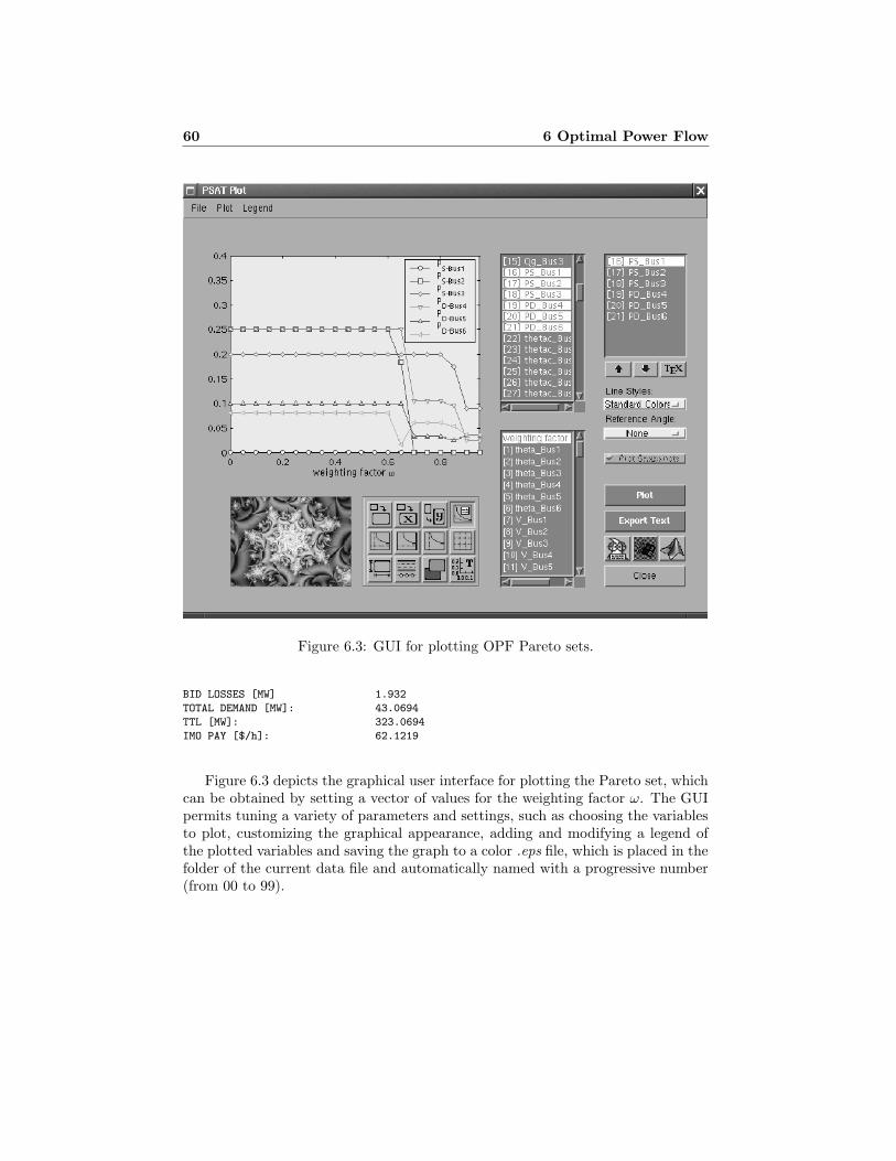
60 6 Optimal Power Flow
Figure 6.3: GUI for plotting OPF Pareto sets.
BID LOSSES [MW] 1.932
TOTAL DEMAND [MW]: 43.0694
TTL [MW]: 323.0694
IMO PAY [$/h]: 62.1219
Figure 6.3 depicts the graphical user interface for plotting the Pareto set, whichcan be obtained by setting a vector of values for the weighting factor ω. The GUIpermits tuning a variety of parameters and settings, such as choosing the variablesto plot, customizing the graphical appearance, adding and modifying a legend ofthe plotted variables and saving the graph to a color .eps file, which is placed in thefolder of the current data file and automatically named with a progressive number(from 00 to 99).

Chapter 7
Small Signal StabilityAnalysis
This chapter describes small signal stability analysis available in PSAT and theassociated graphical user interface. After solving the power flow problem, it ispossible to compute and visualize the eigenvalues and the participation factors ofthe system. The eigenvalues can be computed for the state matrix of the dynamicsystem (small signal stability analysis) [Sauer and Pai 1998, Ilic and Zaborszky2000], and for three different types of power flow Jacobian matrices (QV sensitivityanalysis) [Xu and Mansour 1994].
The following sections describe the main features of the small signal stabilityanalysis and of the power flow Jacobian eigenvalue analysis.
7.1 Small Signal Stability Analysis
The system used for the small signal stability analysis is a differential algebraicequation (DAE) set, in the form:
x = f(x, y) (7.1)
0 = g(x, y)
where x is the vector of the state variables and y the vector of the algebraic variables,which in PSAT are only the voltages amplitudes V and phases θ.
The state matrix AS is thus computed by manipulating the complete Jacobianmatrix AC , that is defined by the linearization of the DAE system equations (7.1):
[∆x0
]=
[∇xf ∇yf∇xg ∇yg
] [∆x∆y
]= [AC ]
[∆x∆y
](7.2)
Hereinafter, the Jacobian matrices which form the AC matrix, will be referred to
61
62 7 Small Signal Stability Analysis
as follows:
Fx , ∇xf (7.3)
Fy , ∇yf
Gx , ∇xg
JLFV , ∇yg
where JLFV is the complete power flow Jacobian matrix. In the program, two othertypes of power flow Jacobian matrices are defined, namely JLF and JLFD, whichare described in the next section.
The state matrix AS is simply obtained by eliminating the algebraic variables,and thus implicitly assuming that JLFV is non-singular (i.e. absence of singularity-induced bifurcations):
AS = Fx − FyJ−1LFV Gx (7.4)
The computation of all eigenvalues can be a lengthy process if the dynamic orderof the system is high. At this aim, it is possible to compute only a few eigenvalueswith a particular property, i.e. largest or smallest magnitude, largest or smallerreal or imaginary part.
When all the eigenvalues are computed, it is also possible to obtain the partic-ipation factors, that are evaluated in the following way. Let V and W be the rightand the left eigenvector matrices respectively, such that Λ = WASV and W = V −1,then the participation factor pij of the ith state variable to the jth eigenvalue canbe defined as:
pij =wijvji
wtjvj
(7.5)
In case of complex eigenvalues, the amplitude of each element of the eigenvectorsis used:
pij =|wij ||vji|∑n
k=1 |wjk||vkj |(7.6)
No normalization of the participation factors is performed.
The state matrix in (7.4) leads to the computation of the eigenvalues in the S-domain, i.e., the system is stable if the real part of the eigenvalues is less than 0. Itis sometime useful to compute the eigenvalues in the Z-domain, which can also easethe visualization of very stiff systems. In this way, if the system is stable, all theeigenvalues are inside the unit circle. For the Z-domain eigenvalue computation, abilinear transformation is performed:
AZ = (AS + ρIn)(AS − ρIn)−1 (7.7)
where ρ is a weighting factor, that in the program is set to 8. Even though moreexpensive, AZ can be useful for fastening the determination of the maximum am-plitude eigenvalue (by means for example of a power method), especially in case ofunstable equilibrium points with only one eigenvalue outside the unit circle.

−6 −5 −4 −3 −2 −1 0−15
−10
−5
0
5
10
15
PSfrag replacements
Real
Imag
Figure 7.1: Eigenvalue Analysis: S-domain.
−1 −0.8 −0.6 −0.4 −0.2 0 0.2 0.4 0.6 0.8 1
−1
−0.8
−0.6
−0.4
−0.2
0
0.2
0.4
0.6
0.8
1
PSfrag replacements
Real
Imag
Figure 7.2: Eigenvalue Analysis: Z-domain.
63

64 7 Small Signal Stability Analysis
7.1.1 Example
The following Figs. 7.1 and 7.2, and the small signal stability report depict theeigenvalue analysis for the WSCC 9-bus test system and have been generated withthe Eigenvalue Analysis interface available in the View menu of the main window.For the static and dynamic data of the network, refer to Subsection F.3.
EIGENVALUE REPORT
P S A T 1.3.4
Author: Federico Milano, (c) 2002-2005e-mail: [email protected]: http://thunderbox.uwaterloo.ca/~fmilano
File: ~/psatd/tests/d_009.mdlDate: 20-Sep-2005 18:52:53
STATE MATRIX EIGENVALUES
Eigevalue Most Associated States Real part Imag. Part Frequency
Eig As 1 vm_Exc_1 -1000 0 0Eig As 2 vm_Exc_1 -1000 0 0Eig As 3 vm_Exc_3 -1000 0 0Eig As 4 delta_Syn_3, omega_Syn_3 -0.72015 12.7454 2.0285Eig As 5 delta_Syn_3, omega_Syn_3 -0.72015 -12.7454 2.0285Eig As 6 omega_Syn_2, delta_Syn_2 -0.19077 8.3657 1.3314Eig As 7 omega_Syn_2, delta_Syn_2 -0.19077 -8.3657 1.3314Eig As 8 vr1_Exc_2, vf_Exc_2 -5.4818 7.9465 1.2647Eig As 9 vr1_Exc_2, vf_Exc_2 -5.4818 -7.9465 1.2647Eig As 10 vr1_Exc_1, vf_Exc_1 -5.2171 7.8127 1.2434Eig As 11 vr1_Exc_1, vf_Exc_1 -5.2171 -7.8127 1.2434Eig As 12 vr1_Exc_3, vf_Exc_3 -5.3181 7.9197 1.2605Eig As 13 vr1_Exc_3, vf_Exc_3 -5.3181 -7.9197 1.2605Eig As 14 e1d_Syn_2 -5.178 0 0Eig As 15 e1d_Syn_3 -3.3996 0 0Eig As 16 e1q_Syn_1, vr2_Exc_1 -0.44307 1.212 0.19289Eig As 17 e1q_Syn_1, vr2_Exc_1 -0.44307 -1.212 0.19289Eig As 18 e1q_Syn_1, e1q_Syn_2 -0.43845 0.74006 0.11778Eig As 19 e1q_Syn_1, e1q_Syn_2 -0.43845 -0.74006 0.11778Eig As 20 e1q_Syn_3, vr2_Exc_3 -0.42503 0.49669 0.07905Eig As 21 e1q_Syn_3, vr2_Exc_3 -0.42503 -0.49669 0.07905Eig As 22 delta_Syn_1 0 0 0Eig As 23 omega_Syn_1 0 0 0Eig As 24 e1d_Syn_1 -3.2258 0 0
PARTICIPATION FACTORS (Euclidean norm)
delta_Syn_1 omega_Syn_1 e1q_Syn_1 e1d_Syn_1 delta_Syn_2
Eig As 1 0 0 0 0 0Eig As 2 0 0 0 0 0Eig As 3 0 0 0 0 0Eig As 4 0.00462 0.00462 1e-05 0 0.08564Eig As 5 0.00462 0.00462 1e-05 0 0.08564Eig As 6 0.12947 0.12947 4e-05 0 0.30889Eig As 7 0.12947 0.12947 4e-05 0 0.30889Eig As 8 0.00021 0.00021 0.00022 0 0.00102Eig As 9 0.00021 0.00021 0.00022 0 0.00102Eig As 10 0.00015 0.00015 0.01789 0 0.00014Eig As 11 0.00015 0.00015 0.01789 0 0.00014Eig As 12 0.00019 0.00019 0.00111 0 4e-05Eig As 13 0.00019 0.00019 0.00111 0 4e-05Eig As 14 2e-05 2e-05 0 0 0.00677
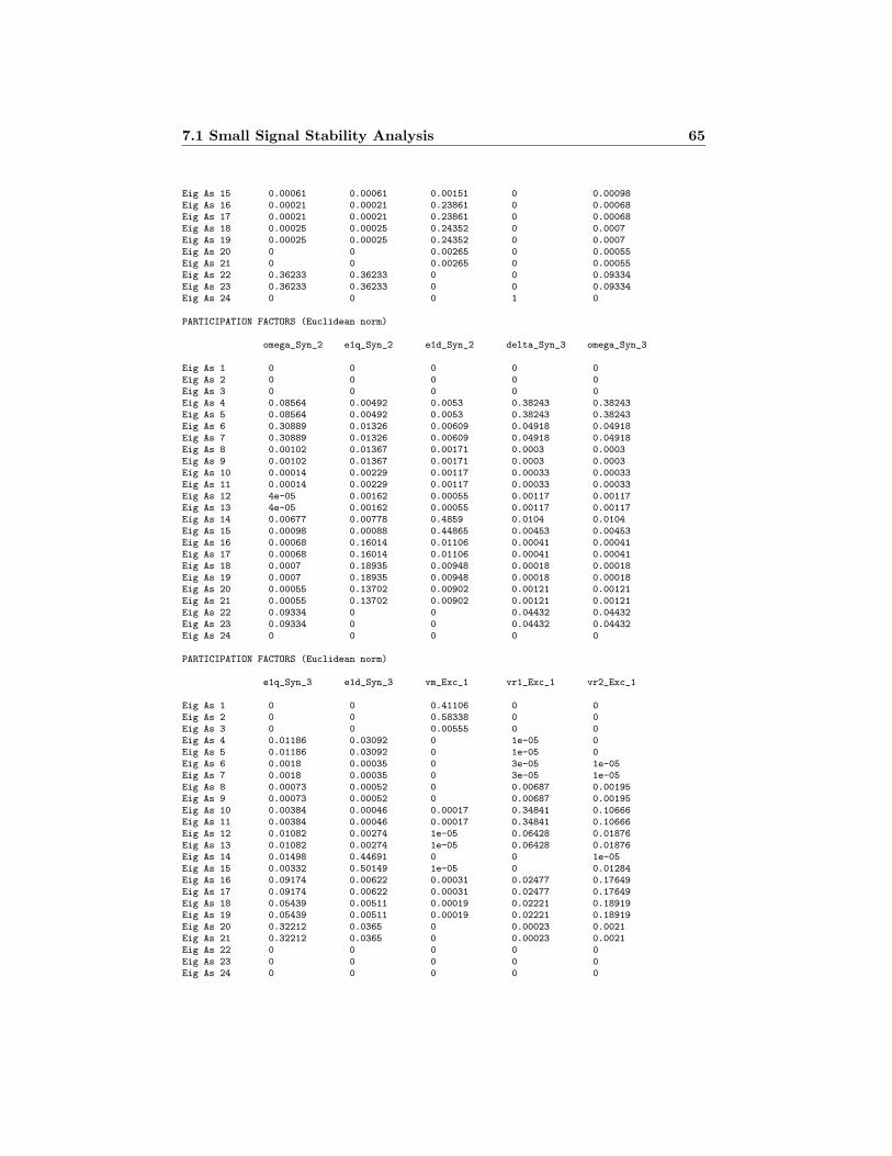
7.1 Small Signal Stability Analysis 65
Eig As 15 0.00061 0.00061 0.00151 0 0.00098Eig As 16 0.00021 0.00021 0.23861 0 0.00068Eig As 17 0.00021 0.00021 0.23861 0 0.00068Eig As 18 0.00025 0.00025 0.24352 0 0.0007Eig As 19 0.00025 0.00025 0.24352 0 0.0007Eig As 20 0 0 0.00265 0 0.00055Eig As 21 0 0 0.00265 0 0.00055Eig As 22 0.36233 0.36233 0 0 0.09334Eig As 23 0.36233 0.36233 0 0 0.09334Eig As 24 0 0 0 1 0
PARTICIPATION FACTORS (Euclidean norm)
omega_Syn_2 e1q_Syn_2 e1d_Syn_2 delta_Syn_3 omega_Syn_3
Eig As 1 0 0 0 0 0Eig As 2 0 0 0 0 0Eig As 3 0 0 0 0 0Eig As 4 0.08564 0.00492 0.0053 0.38243 0.38243Eig As 5 0.08564 0.00492 0.0053 0.38243 0.38243Eig As 6 0.30889 0.01326 0.00609 0.04918 0.04918Eig As 7 0.30889 0.01326 0.00609 0.04918 0.04918Eig As 8 0.00102 0.01367 0.00171 0.0003 0.0003Eig As 9 0.00102 0.01367 0.00171 0.0003 0.0003Eig As 10 0.00014 0.00229 0.00117 0.00033 0.00033Eig As 11 0.00014 0.00229 0.00117 0.00033 0.00033Eig As 12 4e-05 0.00162 0.00055 0.00117 0.00117Eig As 13 4e-05 0.00162 0.00055 0.00117 0.00117Eig As 14 0.00677 0.00778 0.4859 0.0104 0.0104Eig As 15 0.00098 0.00088 0.44865 0.00453 0.00453Eig As 16 0.00068 0.16014 0.01106 0.00041 0.00041Eig As 17 0.00068 0.16014 0.01106 0.00041 0.00041Eig As 18 0.0007 0.18935 0.00948 0.00018 0.00018Eig As 19 0.0007 0.18935 0.00948 0.00018 0.00018Eig As 20 0.00055 0.13702 0.00902 0.00121 0.00121Eig As 21 0.00055 0.13702 0.00902 0.00121 0.00121Eig As 22 0.09334 0 0 0.04432 0.04432Eig As 23 0.09334 0 0 0.04432 0.04432Eig As 24 0 0 0 0 0
PARTICIPATION FACTORS (Euclidean norm)
e1q_Syn_3 e1d_Syn_3 vm_Exc_1 vr1_Exc_1 vr2_Exc_1
Eig As 1 0 0 0.41106 0 0Eig As 2 0 0 0.58338 0 0Eig As 3 0 0 0.00555 0 0Eig As 4 0.01186 0.03092 0 1e-05 0Eig As 5 0.01186 0.03092 0 1e-05 0Eig As 6 0.0018 0.00035 0 3e-05 1e-05Eig As 7 0.0018 0.00035 0 3e-05 1e-05Eig As 8 0.00073 0.00052 0 0.00687 0.00195Eig As 9 0.00073 0.00052 0 0.00687 0.00195Eig As 10 0.00384 0.00046 0.00017 0.34841 0.10666Eig As 11 0.00384 0.00046 0.00017 0.34841 0.10666Eig As 12 0.01082 0.00274 1e-05 0.06428 0.01876Eig As 13 0.01082 0.00274 1e-05 0.06428 0.01876Eig As 14 0.01498 0.44691 0 0 1e-05Eig As 15 0.00332 0.50149 1e-05 0 0.01284Eig As 16 0.09174 0.00622 0.00031 0.02477 0.17649Eig As 17 0.09174 0.00622 0.00031 0.02477 0.17649Eig As 18 0.05439 0.00511 0.00019 0.02221 0.18919Eig As 19 0.05439 0.00511 0.00019 0.02221 0.18919Eig As 20 0.32212 0.0365 0 0.00023 0.0021Eig As 21 0.32212 0.0365 0 0.00023 0.0021Eig As 22 0 0 0 0 0Eig As 23 0 0 0 0 0Eig As 24 0 0 0 0 0
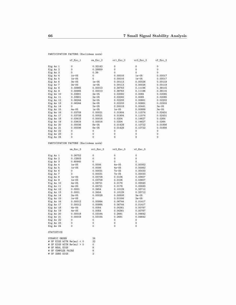
66 7 Small Signal Stability Analysis
PARTICIPATION FACTORS (Euclidean norm)
vf_Exc_1 vm_Exc_2 vr1_Exc_2 vr2_Exc_2 vf_Exc_2
Eig As 1 0 0.32142 0 0 0Eig As 2 0 0.28859 0 0 0Eig As 3 0 0.39 0 0 0Eig As 4 1e-05 0 0.00016 1e-05 0.00017Eig As 5 1e-05 0 0.00016 1e-05 0.00017Eig As 6 3e-05 1e-05 0.00113 0.00026 0.00119Eig As 7 3e-05 1e-05 0.00113 0.00026 0.00119Eig As 8 0.00665 0.00013 0.38763 0.11196 0.38115Eig As 9 0.00665 0.00013 0.38763 0.11196 0.38115Eig As 10 0.33901 2e-05 0.02092 0.0065 0.02065Eig As 11 0.33901 2e-05 0.02092 0.0065 0.02065Eig As 12 0.06244 2e-05 0.02233 0.00661 0.02202Eig As 13 0.06244 2e-05 0.02233 0.00661 0.02202Eig As 14 0 2e-05 0.00018 0.00441 3e-05Eig As 15 4e-05 1e-05 1e-05 0.00889 3e-05Eig As 16 0.03708 0.00021 0.01904 0.11574 0.02431Eig As 17 0.03708 0.00021 0.01904 0.11574 0.02431Eig As 18 0.03415 0.00016 0.0204 0.14627 0.0264Eig As 19 0.03415 0.00016 0.0204 0.14627 0.0264Eig As 20 0.00036 8e-05 0.01429 0.10722 0.01856Eig As 21 0.00036 8e-05 0.01429 0.10722 0.01856Eig As 22 0 0 0 0 0Eig As 23 0 0 0 0 0Eig As 24 0 0 0 0 0
PARTICIPATION FACTORS (Euclidean norm)
vm_Exc_3 vr1_Exc_3 vr2_Exc_3 vf_Exc_3
Eig As 1 0.26752 0 0 0Eig As 2 0.12803 0 0 0Eig As 3 0.60445 0 0 0Eig As 4 1e-05 0.0006 4e-05 0.00062Eig As 5 1e-05 0.0006 4e-05 0.00062Eig As 6 0 0.00031 7e-05 0.00033Eig As 7 0 0.00031 7e-05 0.00033Eig As 8 1e-05 0.03708 0.0106 0.03607Eig As 9 1e-05 0.03708 0.0106 0.03607Eig As 10 4e-05 0.05721 0.0176 0.05593Eig As 11 4e-05 0.05721 0.0176 0.05593Eig As 12 0.0001 0.3454 0.10129 0.33712Eig As 13 0.0001 0.3454 0.10129 0.33712Eig As 14 2e-05 0.00028 0.00508 3e-05Eig As 15 1e-05 0 0.01006 3e-05Eig As 16 0.00012 0.00994 0.06744 0.01417Eig As 17 0.00012 0.00994 0.06744 0.01417Eig As 18 4e-05 0.0054 0.04361 0.00787Eig As 19 4e-05 0.0054 0.04361 0.00787Eig As 20 0.00018 0.03164 0.2681 0.04642Eig As 21 0.00018 0.03164 0.2681 0.04642Eig As 22 0 0 0 0Eig As 23 0 0 0 0Eig As 24 0 0 0 0
STATISTICS
DYNAMIC ORDER 24# OF EIGS WITH Re(mu) < 0 22# OF EIGS WITH Re(mu) > 0 0# OF REAL EIGS 8# OF COMPLEX PAIRS 8# OF ZERO EIGS 2

7.2 QV Sensitivity Analysis 67
7.2 QV Sensitivity Analysis
For the eigenvalue analysis of the power flow Jacobian matrices, three matrices canbe used:
1. JLF , which is obtained from the static equations (10.1) of only lines andtransformers, and is generally defined as the standard power flow Jacobianmatrix;
2. JLFV , which is the Jacobian of the complete Jacobian matrix of the algebraicequations of the system;
3. JLFD, which is computed from the complete matrix AC :
JLFD = JLFV −GyF−1x Fy (7.8)
and can thus be considered a kind of dynamic power flow Jacobian matrix. Ifthere are pure integrators in the system, Fx can be singular. In this case, Fx
is conditioned by adding a small value on the diagonal before computing theinverse.
After selecting the power flow Jacobian matrix, the eigenvalue analysis is performedon a reduced matrix, as follows. Let’s assume that the power flow Jacobian matrixis divided in four sub-matrices:
JLF =
[JPθ JPV
JQθ JQV
](7.9)
In case of the standard Jacobian matrix JLF , this has also a physical meaning, sinceit can be obtained by the linearization of the power flow equations with constantpower injections: [
∆P∆Q
]=
[JPθ JPV
JQθ JQV
] [∆θ∆V
](7.10)
Then, the reduced matrix is defined as follows:
JLFr = JQV − JQθJ−1Pθ JPV (7.11)
That can thus be used for a QV sensitivity analysis, if one assumes that ∆P = 0and that the sub-matrix JPθ is non-singular:
∆Q = JLFr∆V (7.12)
For JLFV and JLFD, the reduced matrix is defined as in (7.11), even though itlacks the rigorous physical meaning of (7.12).
7.2.1 Example
The following Fig. 7.3 and QV sensitivity report depicts the QV sensitivity analysisfor the IEEE 14-bus test system and have been generated with the GUI for Small

68 7 Small Signal Stability Analysis
0 10 20 30 40 50 60 70−1
−0.8
−0.6
−0.4
−0.2
0
0.2
0.4
0.6
0.8
1
PSfrag replacements
Real
Imag
Figure 7.3: Eigenvalue Analysis: QV sensitivity.
Signal Stability Analysis available in the View menu of the main window. For thestatic data of the network, refer to Section F.4. The report refers to the JLF matrix,but since the system has only constant power loads and generators and there areno dynamic components, one has JLF = JLFV = JLFD. The report shows fivehigh eigenvalues (µ = 999), which represent the constant voltage buses of the fivegenerators.
EIGENVALUE REPORT
P S A T 1.3.0
Author: Federico Milano, (c) 2002-2004e-mail: [email protected]: http://thunderbox.uwaterloo.ca/~fmilano
File: ~/psatd/tests/d_014.mdlDate: 16-Mar-2004 14:47:53
EIGENVALUES OF THE COMPLETE POWER JACOBIAN MATRIX
Eigevalue Real part Imaginary Part
Eig Jlfv1 64.9803 0Eig Jlfv2 39.2929 0Eig Jlfv3 21.7272 0Eig Jlfv4 18.8536 0Eig Jlfv5 16.2706 0Eig Jlfv6 2.6984 0Eig Jlfv7 5.5274 0Eig Jlfv8 7.6017 0

7.2 QV Sensitivity Analysis 69
Eig Jlfv9 11.2207 0Eig Jlfv10 999 0Eig Jlfv11 999 0Eig Jlfv12 999 0Eig Jlfv13 999 0Eig Jlfv14 999 0
PARTICIPATION FACTORS (Euclidean norm)
Bus 01 Bus 02 Bus 03 Bus 04 Bus 05
Eig Jlfv1 0 0 0 0.53957 0.45377Eig Jlfv2 0 0 0 3e-05 0.00065Eig Jlfv3 0 0 0 0.07934 0.15554Eig Jlfv4 0 0 0 0.00038 0.00048Eig Jlfv5 0 0 0 0.28196 0.31696Eig Jlfv6 0 0 0 0.00823 0.00397Eig Jlfv7 0 0 0 0.00246 0.00136Eig Jlfv8 0 0 0 1e-05 0Eig Jlfv9 0 0 0 0.08802 0.06726Eig Jlfv10 1 0 0 0 0Eig Jlfv11 0 1 0 0 0Eig Jlfv12 0 0 1 0 0Eig Jlfv13 0 0 0 0 0Eig Jlfv14 0 0 0 0 0
PARTICIPATION FACTORS (Euclidean norm)
Bus 06 Bus 07 Bus 08 Bus 09 Bus 10
Eig Jlfv1 0 0.00653 0 0.00012 1e-05Eig Jlfv2 0 0.1549 0 0.61494 0.21327Eig Jlfv3 0 0.49063 0 0.00357 0.21787Eig Jlfv4 0 0.00013 0 0.00015 0.00443Eig Jlfv5 0 0.02216 0 0.04693 0.16526Eig Jlfv6 0 0.0691 0 0.19882 0.2394Eig Jlfv7 0 0.01672 0 0.03173 0.11939Eig Jlfv8 0 3e-05 0 4e-05 0.0364Eig Jlfv9 0 0.23981 0 0.10371 0.00396Eig Jlfv10 0 0 0 0 0Eig Jlfv11 0 0 0 0 0Eig Jlfv12 0 0 0 0 0Eig Jlfv13 1 0 0 0 0Eig Jlfv14 0 0 1 0 0
PARTICIPATION FACTORS (Euclidean norm)
Bus 11 Bus 12 Bus 13 Bus 14
Eig Jlfv1 0 0 0 0Eig Jlfv2 0.00759 0 0.00012 0.0085Eig Jlfv3 0.05254 3e-05 0.00018 0.00031Eig Jlfv4 0.00192 0.17934 0.766 0.04716Eig Jlfv5 0.15559 0.0022 0.00499 0.00395Eig Jlfv6 0.11026 0.01886 0.03232 0.31905Eig Jlfv7 0.13155 0.32558 0.16032 0.2109Eig Jlfv8 0.11208 0.46399 0.03394 0.3535Eig Jlfv9 0.42848 0.01 0.00213 0.05664Eig Jlfv10 0 0 0 0Eig Jlfv11 0 0 0 0Eig Jlfv12 0 0 0 0Eig Jlfv13 0 0 0 0Eig Jlfv14 0 0 0 0
STATISTICS
NUMBER OF BUSES 14# OF EIGS WITH Re(mu) < 0 0
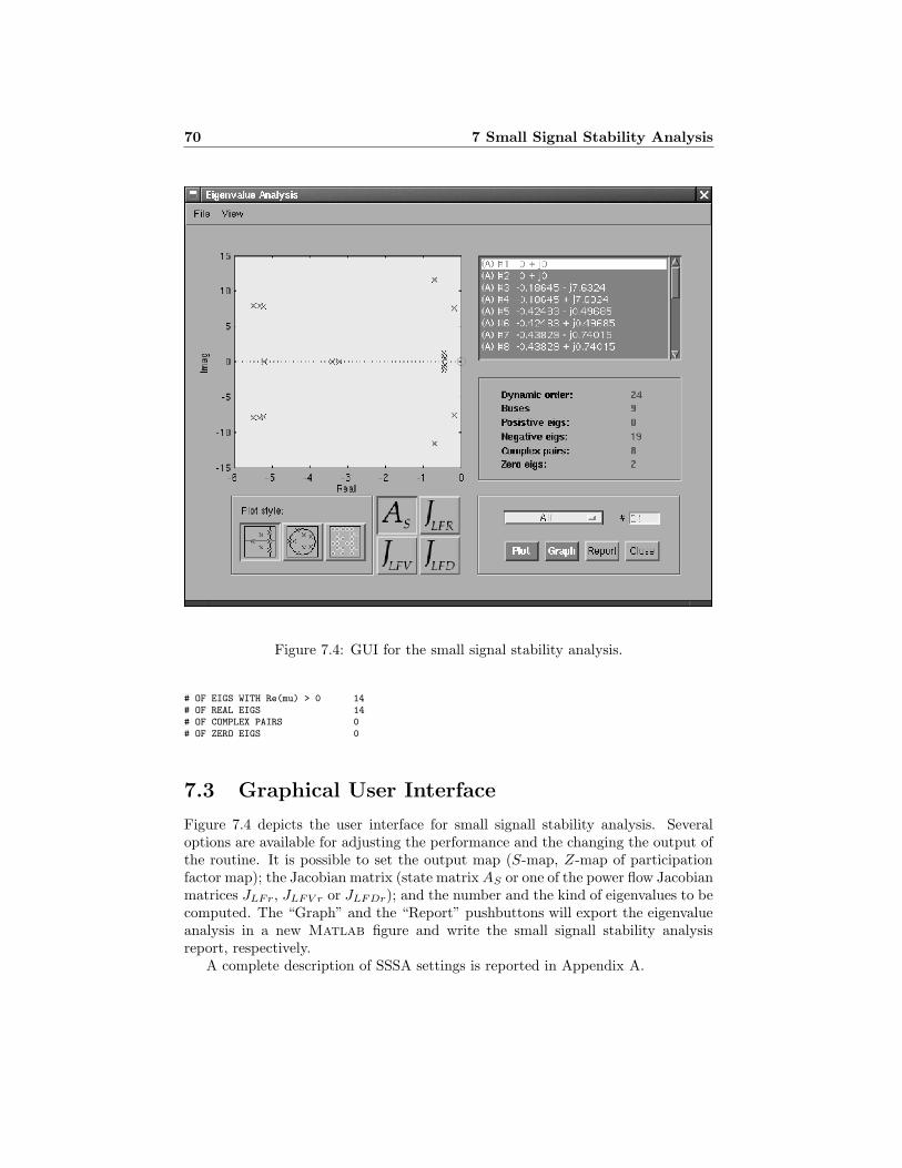
70 7 Small Signal Stability Analysis
Figure 7.4: GUI for the small signal stability analysis.
# OF EIGS WITH Re(mu) > 0 14# OF REAL EIGS 14# OF COMPLEX PAIRS 0# OF ZERO EIGS 0
7.3 Graphical User Interface
Figure 7.4 depicts the user interface for small signall stability analysis. Severaloptions are available for adjusting the performance and the changing the output ofthe routine. It is possible to set the output map (S-map, Z-map of participationfactor map); the Jacobian matrix (state matrix AS or one of the power flow Jacobianmatrices JLFr, JLFV r or JLFDr); and the number and the kind of eigenvalues to becomputed. The “Graph” and the “Report” pushbuttons will export the eigenvalueanalysis in a new Matlab figure and write the small signall stability analysisreport, respectively.
A complete description of SSSA settings is reported in Appendix A.
Chapter 8
Time Domain Simulation
This chapter describes the time domain integration methods used in PSAT and theirsettings. A particular class of settings are the snapshots that allows computingspecific points during the time simulations. How to include disturbances is alsodescribed in this chapter. Three phase faults and breaker operations are supportedby means of specific functions and structures, while a generic disturbance can becreated writing an user defined function. Finally, the plotting utilities for timedomain simulations are briefly described by means of simple examples.
Observe that several programs for power system analysis make a distinctionbetween power flow (static) data and dynamic ones. On the contrary, in PSAT,static and dynamic data can be defined in the same data file. Then PSAT makesuse of static and/or dynamic data depending on the kind of the currently runningsimulation.
8.1 Integration Methods
Two integration methods are available, i.e. forward Euler and trapezoidal rule,which are implicit A-stable algorithms and use a complete Jacobian matrix toevaluate the algebraic and state variable directions at each step. These methodsare well known and can be found in many books (e.g. [Brenan et al. 1995]).
For a generic time t, and assumed a time step ∆t, one has to solve the followingproblem:
0 = fn(x(t+ ∆t), y(t+ ∆t), f(t)) (8.1)
0 = g(x(t+ ∆t), y(t+ ∆t))
where f and g represent the differential and algebraic equations and fn is a functionthat depends on the integration method. Equations (8.1) are nonlinear and theirsolution is obtained by means of a Newton-Raphson technique which in turn consistsof computing iteratively the increment ∆xi and ∆yi of the state and algebraic
71

72 8 Time Domain Simulation
variables and updating the actual variables:[∆xi
∆yi
]= −[Ai
c]−1
[f i
n
gi
](8.2)
[xi+1
yi+1
]=
[xi
yi
]+
[∆xi
∆yi
]
where Aic is a matrix depending on the algebraic and state Jacobian matrices of the
system. The loop stops if the variable increment is below a certain fixed toleranceε0 or if the maximum number of iteration is reached. In the latter case the timestep ∆t is reduced and the Newton-Raphson technique repeated again. Figure 8.1depicts the block diagram of the time domain integration. For sake of completeness,the following sections report the expressions of Ai
c and f in for each method.
8.1.1 Forward Euler Method
The forward Euler integration method is a first order method. It is generally fasterbut less accurate than the trapezoidal method. At a generic iteration i, Ai
c and f in
are as follows:
Aic =
[In − ∆tF i
x −∆tF iy
Gix J i
LFV
](8.3)
f in = xi − x(t) − ∆tf i
where In is the identity matrix of the same dimension of the dynamic order of thesystem, and the other matrices are the Jacobian matrices of the algebraic differentialequations, i.e. Fx = ∇xf , Fy = ∇yf , Gx = ∇xg and JLFV = ∇yg.
8.1.2 Trapezoidal Method
The trapezoidal method is the workhorse solver for electro-mechanical DAE, andis widely used, in a variety of flavors, in most commercial and non-commercialpower system software packages. The version implemented in PSAT is probablythe simplest one, but proved to be very robust and reliable for several test cases.At a generic iteration i, Ai
c and f in are as follows:
Aic =
[In − 0.5∆tF i
x −0.5∆tF iy
Gix J i
LFV
](8.4)
f in = xi − x(t) − 0.5∆t(f i + f(t))
where the notation is the same as in (8.3).
8.2 Settings
General settings for time domain simulations, i.e. the initial1 and final times,convergence tolerance, and maximum number of iterations of the Newton-Raphson
1Although the initial time could be assigned any value, it is recommended to use t0 = 0 asother values have not been tested. In any case it must be t0 > 0.

PSfrag replacements
END
END
Singularity
likely
Integration
method
Compute
Evaluate
Evaluate system
Evaluate initial
Power Flow &
Initial State Variables
equations & Jacobians
disturbance
OutputUpdate x & y
Recompute
time step ∆t
t = t0
i = 0
i = i+ 1
Reduce ∆ti > imax ∆t < ∆tmin
∆t
∆x and ∆y
|∆xi|, |∆yi| < ε
t+ ∆t ≥ tf
yes
yes
yes
yes
no
no
no
no
Figure 8.1: Time domain integration block diagram.
73

74 8 Time Domain Simulation
technique for each time step can be set in the main window. Other parameterscan be customized in the GUI for general settings (menu Edit/General Settings orshortcut <Ctr-k> in the main window), which is depicted in Fig. 8.2. The followingoptions are available for time domain simulations:
Fixed Time Step: one can enable the use of a fixed time step. this can be useful for“critical” simulations were the automatic time step flaws. If the option of thefixed time step is disabled, PSAT will computes a reasonable initial time stepbased on the eigenvalues of the system at the initial time.2 Observe that thisprocedure can be time-consuming for systems with an high number of statevariables.
Time Step [s]: the value of the time step in seconds. The default value is 0.001 s.
Integration Method: one can choose in between Trapezoidal Rule (default) and For-ward Euler. Both methods are implicit and A-stable. The trapezoidal rule isthe workhorse of time domain simulations of power electric systems.
Stop TDs at Max Delta: this option makes possible to stop the time domain sim-ulation when the maximum machine angle difference is greater than a given∆δmax.
3
Max. Delta Diff. [deg]: the maximum machine angle difference in degree for whichthe time domain simulation will be stopped. The default value is 180.
Convert PQ bus to Z: if this option is enabled, PQ buses are converted to constantimpedances right before beginning the time domain simulation. This will helpconvergence if there are fault occurrences and breaker interventions during thetime domain simulation. Refer to Sections 10.6 and 14.1 for details on theconversion of PQ loads to constant impedances.
Plot during Simulation: to enforce this option will generate a graphic of selectedvariables (see item Plotting Variables) during time domain simulations. it istypically a time consuming operation and it is disabled by default.
Plotting Variables: this pop-up menu allows selecting plotting variables that willbe displayed during time domain simulations. Observe that these are not thevariables that will be stored in the output. See Section 8.3 for more detailson output variable selection.
Update Simulink during TD: this option allows displaying and updating voltagesin Simulink models during time domain simulations. this option only worksif the data are loaded from a Simulink model. This option won’t work if onOctave and for the command line usage of PSAT.
Settings for time domain simulations are stored in the structure Settings, whichcontains also general settings and parameters for power flow computations. Thisstructure is fully described in Appendix A.
2this operation is performed in the function fm tstep.3This option has been added by Laurent Lenoir, Ecole Polytechnique de Montreal.

Figure 8.2: GUI for general settings.
75

76 8 Time Domain Simulation
8.3 Output Variable Selection
During time domain simulations (and also for CPF analysis), PSAT stores outputvariables in the structure Varout. Further details on this structure are given in theAppendix A.
By default, PSAT stores only state variables, bus voltage magnitudes and busvoltage angles. This behavior can be changed by means of the GUI for plot variableselection (see Fig. 8.3). By this GUI, the user can select any of the followingvariables:
1. State variables;
2. Bus voltage magnitudes and angles;
3. Bus voltage angles;
4. Generator mechanical powers and field voltages;
5. AVR reference voltages;
6. Over-excitation limiter currents.
7. Active and reactive power injections at buses;
8. Active and reactive power flows in transmission lines;
The selection must be done after running the power flow analysis and beforerunning the time domain simulation.
The GUI allows selecting variables one by one or by packages. When usingthe command line version of PSAT, selection can be done by assigning a vector ofindexes to Varout.idx. The variable indexes are as follows:
- from (1) to (DAE.n) state variables.
- from (DAE.n + 1) to (DAE.n + Bus.n) bus voltage magnitudes.
- from (DAE.n + Bus.n + 1) to (DAE.n + 2*Bus.n) bus voltage angles.
- from (DAE.n + 2*Bus.n + 1) to (DAE.n + 2*Bus.n + Syn.n) generator me-chanical powers.
- from (DAE.n + 2*Bus.n + Syn.n + 1) to (DAE.n + 2*Bus.n + 2*Syn.n) gen-erator field voltages.
- from (DAE.n + 2*Bus.n + 2*Syn.n + 1) to (DAE.n + 2*Bus.n + 2*Syn.n
+ Exc.n) AVR reference voltages.
- from (DAE.n + 2*Bus.n + 2*Syn.n + Exc.n + 1) to (DAE.n + 2*Bus.n +
2*Syn.n + Exc.n + Oxl.n) OXL currents.
- from (DAE.n + 2*Bus.n + 2*Syn.n + Exc.n + Oxl.n + 1) to (DAE.n + 3*Bus.n
+ 2*Syn.n + Exc.n + Oxl.n) active power injections at buses.
8.4 Snapshots 77
- from (DAE.n + 3*Bus.n + 2*Syn.n + Exc.n + Oxl.n + 1) to (DAE.n + 4*Bus.n
+ 2*Syn.n + Exc.n + Oxl.n) reactive power injections at buses.
- from (DAE.n + 4*Bus.n + 2*Syn.n + Exc.n + Oxl.n + 1) to (DAE.n + 4*Bus.n
+ 2*Syn.n + Exc.n + Oxl.n + Line.n) active power flows i-j.
- from (DAE.n + 4*Bus.n + 2*Syn.n + Exc.n + Oxl.n + Line.n + 1) to (DAE.n+ 4*Bus.n + 2*Syn.n + Exc.n + Oxl.n + 2*Line.n) reactive power flowsi-j.
- from (DAE.n + 4*Bus.n + 2*Syn.n + Exc.n + Oxl.n + 2*Line.n + 1) to(DAE.n + 4*Bus.n + 2*Syn.n + Exc.n + Oxl.n + 3*Line.n) active powerflows j-i.
- from (DAE.n + 4*Bus.n + 2*Syn.n + Exc.n + Oxl.n + 3*Line.n + 1) to(DAE.n + 4*Bus.n + 2*Syn.n + Exc.n + Oxl.n + 4*Line.n) active powerflows j-i.
For example if one wants to plot only the voltage magnitude of the third busand the active power injections at the fourth bus, the index assignment will be asfollows:
>> Varout.idx = [DAE.n+3, DAE.n+2*Bus.n+2*Syn.n+Exc.n+Oxl.n+4];
The assignment must be done after running the power flow analysis and beforerunning the time domain simulation. If this assignment is done in a function,remember to declare as global all needed structures.
8.4 Snapshots
Figure 8.4 depicts the graphical user interface for setting the snapshots (menuTools/Snapshots or shortcut <Ctr-n> in the main window). This GUI is displayedonly after solving the power flow and always contains a snapshot called Power FlowResult. The GUI allows to set any number of snapshots at desired times. Whenrunning the time domain simulation, the integration routine will compute a pointfor each time defined in the snapshots and store the system variables in the structureSnapshot. This option can be useful for being sure that the time domain simulationwill compute a point for a determined time at which a disturbance is applied or forfitting the time steps in delimited regions of the simulation time interval.
The GUI allows also to set the currently selected snapshot as the “initial time”for the next time domain simulation. This option allows starting the time domainsimulation without actually recomputing the power flow. A snapshot defined asinitial time can be visualized by the GUI for power flow reports (menu View/StaticReport or shortcut <Ctr-v> in the main window). A sequence of snapshots can bealso visualized in the GUI for plotting variables (menu View/Plotting Utilities orshortcut <Ctr-w> in the main window).

Figure 8.3: GUI for plot variable selection.
78
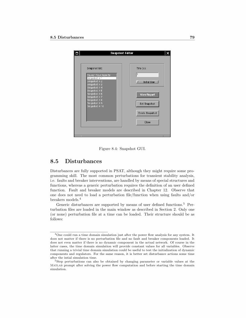
8.5 Disturbances 79
Figure 8.4: Snapshot GUI.
8.5 Disturbances
Disturbances are fully supported in PSAT, although they might require some pro-gramming skill. The most common perturbations for transient stability analysis,i.e. faults and breaker interventions, are handled by means of special structures andfunctions, whereas a generic perturbation requires the definition of an user definedfunction. Fault and breaker models are described in Chapter 12. Observe thatone does not need to load a perturbation file/function when using faults and/orbreakers models.4
Generic disturbances are supported by means of user defined functions.5 Per-turbation files are loaded in the main window as described in Section 2. Only one(or none) perturbation file at a time can be loaded. Their structure should be asfollows:
4One could run a time domain simulation just after the power flow analysis for any system. Itdoes not matter if there is no perturbation file and no fault and breaker components loaded. Itdoes not even matter if there is no dynamic component in the actual network. Of course in thelatter cases, the time domain simulation will provide constant values for all variables. Observethat running a trivial time domain simulation could be useful to test the initialization of dynamiccomponents and regulators. For the same reason, it is better set disturbance actions some timeafter the intial simulation time.
5Step perturbations can also be obtained by changing parameter or variable values at theMatlab prompt after solving the power flow computation and before starting the time domainsimulation.

80 8 Time Domain Simulation
function pert(t)
global global_variable_name1 global_variable_name2 ...
if ... % criterion
% actions
elseif ... % criterion
% actions
else
% actions
end
The function must accept as an input the current simulation time (scalar value)and may include any global structure of the system for taking the desired actions.6
Observe that the time domain integration calls the disturbance file at each iteration,thus it may be convenient to reduce the number of operations within the disturbancefunction. In order to force the integration routine to evaluate a particular point,define the desired time in the Snapshot structure.
8.6 Examples
Figure 8.5 depicts the graphical user interface for plotting time domain simulationresults. As an example the figure depicts the speeds ω for the three generators ofthe WSCC 9-bus test system. Generators are represented by means of a fourthorder model with automatic voltage regulation (IEEE type I) [Sauer and Pai 1998].The data for this system are reported in Appendix F.3. After solving the powerflow, the rotor speed of one generator is set to 0.95 p.u. as follows:
>> DAE.x(Syn.omega(2)) = 0.95;
then the time domain simulation is performed. The GUI allows a variety of settings,such as choosing the variables to plot, setting in detail the graphical appearance,adding and modifying a legend of the plotted variables and saving the graph to acolor .eps file, which is placed in the folder of the current data file and automaticallynamed with a progressive number (from 00 to 99).
Figures 8.6, 8.7, and 8.8 depict generator speeds, generator rotor angles and busvoltages for the 9-bus test system with simplified synchronous machine models (δ, ω
6Observe that it may be necessary to call other functions. For example, after modifying atransmission line impedance, one has to call fm y in order to rebuild the admittance matrix.

Figure 8.5: GUI for plotting time domain simulations. In this example, the speedsrefer to the 9-bus test with IV order generator models and AVRs type II. Theperturbance is obtained by varying the speed of generator 2 at the Matlab prompt(ω2(t0) = 0.95 p.u.).
81

82 8 Time Domain Simulation
0 1 2 3 4 5 6 71
1.005
1.01
1.015
1.02
1.025
1.03
1.035
1.04
1.045
PSfrag replacements
Rot
orSpee
ds
[p.u
.]
ωGen 1ωGen 2ωGen 3
Time [s]
Figure 8.6: Generator speeds for the 9-bus test system with II order generatormodels and a fault applied at bus 7.
model), as described in the examples 2.6-2.7, pp. 41-46, “Power System Controland Stability”, by P. M. Anderson and A. A. Fouad [Anderson and Fouad 1977]. Athree phase fault occurs at t = 1 s, at bus 7. The fault is then cleared by openingthe line 4-7 at t = 1.083 s. Finally the line 4-7 is reclosed at t = 4 s. The data forthis system are reported as well in Appendix F.3.

0 1 2 3 4 5 6 70
5
10
15
20
25
30
35
40
PSfrag replacements
Rot
orA
ngl
es[rad
]
δGen 1δGen 2δGen 3
Time [s]
Figure 8.7: Generator rotor angles for the 9-bus test system with II order generatormodels and a fault applied at bus 7.
83

0 1 2 3 4 5 6 70
0.2
0.4
0.6
0.8
1
PSfrag replacements Vol
tage
s[p
.u.]
Time [s]
VBus 1VBus 2VBus 3VBus 4VBus 5VBus 6VBus 7VBus 8VBus 9
Figure 8.8: Bus voltages for the 9-bus test system with II order generator modelsand a fault applied at bus 7.
84

Chapter 9
PMU Placement
This chapter describes seven methods for Phasor Measurement Unit (PMU) place-ment with the aim of linear static state estimation of power system networks. Thesemethods are depth first, graph theoretic procedures and bisecting search-simulatedannealing which were proposed in [Baldwin et al. 1993], as well as recursive andsingle shot N security and recursive and single shot N-1 security algorithms whichwere proposed in [Denegri et al. 2002]. A description of the PMU placement GUIand an example of report file for the 14-bus test system are reported at the end ofthis chapter.
9.1 Linear Static State Estimation
This section briefly describes basic concepts of power system static state estimationbased on what was proposed in [Schweppe et al. 1970] and [Clements et al. 1981].
The static state estimation problem is generally formulated as a non-linear setof equations, as follows:
z = h(x) + ε (9.1)
where:
z (z ∈ Rm): measurement vector;
x (x ∈ Rn): state vector;
ε (ε ∈ Rm): measurement errors vector;
h (h : Rn → R
m): vector of the relationships between states and measurements;
Equation (9.1) is typically solved by means of a Newton-Raphson technique [Sch-weppe et al. 1970, Allemong et al. 1982, Monticelli and Garcia 1990]. Using devicesable to provide voltage and current phasors, such as PMUs, yields a linear relation-ship between state variables and measurements variables, as follows:
z = Hx+ ε (9.2)
85
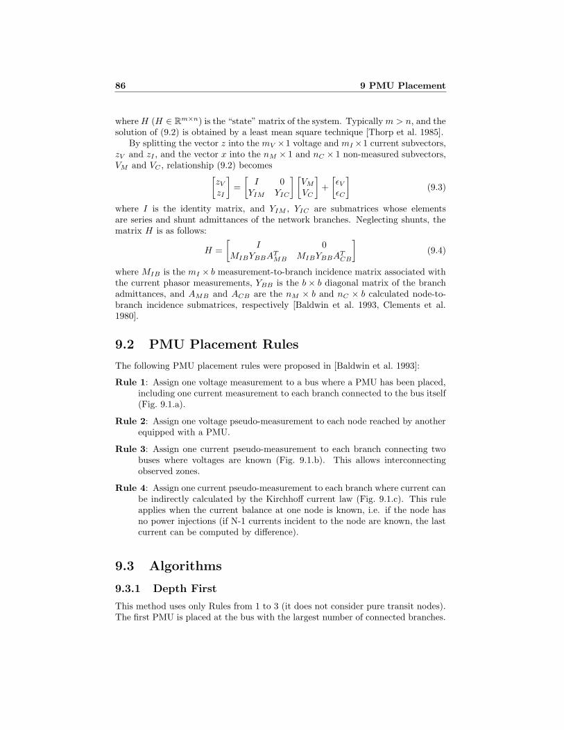
86 9 PMU Placement
whereH (H ∈ Rm×n) is the “state” matrix of the system. Typicallym > n, and the
solution of (9.2) is obtained by a least mean square technique [Thorp et al. 1985].By splitting the vector z into the mV ×1 voltage and mI ×1 current subvectors,
zV and zI , and the vector x into the nM × 1 and nC × 1 non-measured subvectors,VM and VC , relationship (9.2) becomes
[zV
zI
]=
[I 0
YIM YIC
] [VM
VC
]+
[εVεC
](9.3)
where I is the identity matrix, and YIM , YIC are submatrices whose elementsare series and shunt admittances of the network branches. Neglecting shunts, thematrix H is as follows:
H =
[I 0
MIBYBBATMB MIBYBBA
TCB
](9.4)
where MIB is the mI × b measurement-to-branch incidence matrix associated withthe current phasor measurements, YBB is the b × b diagonal matrix of the branchadmittances, and AMB and ACB are the nM × b and nC × b calculated node-to-branch incidence submatrices, respectively [Baldwin et al. 1993, Clements et al.1980].
9.2 PMU Placement Rules
The following PMU placement rules were proposed in [Baldwin et al. 1993]:
Rule 1: Assign one voltage measurement to a bus where a PMU has been placed,including one current measurement to each branch connected to the bus itself(Fig. 9.1.a).
Rule 2: Assign one voltage pseudo-measurement to each node reached by anotherequipped with a PMU.
Rule 3: Assign one current pseudo-measurement to each branch connecting twobuses where voltages are known (Fig. 9.1.b). This allows interconnectingobserved zones.
Rule 4: Assign one current pseudo-measurement to each branch where current canbe indirectly calculated by the Kirchhoff current law (Fig. 9.1.c). This ruleapplies when the current balance at one node is known, i.e. if the node hasno power injections (if N-1 currents incident to the node are known, the lastcurrent can be computed by difference).
9.3 Algorithms
9.3.1 Depth First
This method uses only Rules from 1 to 3 (it does not consider pure transit nodes).The first PMU is placed at the bus with the largest number of connected branches.

9.3 Algorithms 87
PSfrag replacements
(a) (b) (c)
pure transit node
Figure 9.1: PMU placement rules.
If there is more than one bus with this characteristic, one is randomly chosen.Following PMUs are placed with the same criterion, until the complete networkobservability is obtained, as depicted in Fig. 9.2.1
9.3.2 Graph Theoretic Procedure
This method was originally proposed in [Baldwin et al. 1993] and is similar to thedepth first algorithm, except for taking into account pure transit nodes (Rule 4).
9.3.3 Bisecting Search Method
Figures 9.3 and 9.4 depict the flowchart of the bisecting search method and thepseudo-code of the simulated annealing procedure. Refer to [Baldwin et al. 1993]for the complete description of this method.
9.3.4 Recursive Security N Algorithm
This method is a modified depth first approach. The procedure can be subdividedinto three main steps:
a) Generation of N minimum spanning trees: Fig. 9.5 depicts the flow chartof the minimum spanning tree generation algorithm. The algorithm is per-formed N times (N being the number of buses), using as starting bus eachbus of the network.
b) Search of alternative patterns: The PMU sets obtained with the step (a)are reprocessed as follows: one at a time, each PMU of each set is replacedat the buses connected with the node where a PMU was originally set, asdepicted in Fig. 9.6. PMU placements which lead to a complete observabilityare retained.
c) Reducing PMU number in case of pure transit nodes: In this step it isverified if the network remains observable taking out one PMU at a time fromeach set, as depicted in Fig. 9.7. If the network does not present pure transitnodes, the procedure ends at step (b).
1The depth first and the graph theoretic procedures do not ensure a minimum PMU placement.

88 9 PMU Placement
PSfrag replacements
Start
End
Yes
No
Place a PMU at the bus
with the most branches
in the unobservable region
Determine the system’s
coverage with the placed
PMU’s
Is the
system observable?
Figure 9.2: Flowchart of the Graph Theoretic Procedure.
The placement sets which present the minimum number of PMUs are finally se-lected.
9.3.5 Single Shot Security N Algorithm
This method was proposed in [Denegri et al. 2002]. The algorithm is based only ontopological rules, and determines a single spanning tree, as illustrated in Fig. 9.8.
9.3.6 Recursive and Single-Shot Security N-1 Algorithms
The rules for minimal PMU placement assume a fixed network topology and acomplete reliability of measurement devices. Simple criteria which yield a completeobservability in case of line outages (N-1 security) are proposed in [Denegri et al.2002] and are based on the following definition: A bus is said to be observable if atleast one of the two following conditions applies:
Rule 1: a PMU is placed at the node;
Rule 2: the node is connected at least to two nodes equipped with a PMU.
Rule 2 is ignored if the bus is connected to single-end line. Figures 9.9 and 9.10depict the algorithms for obtaining the N-1 security placement proposed in [Denegriet al. 2002]. The first method is a slightly different version of the recursive technique
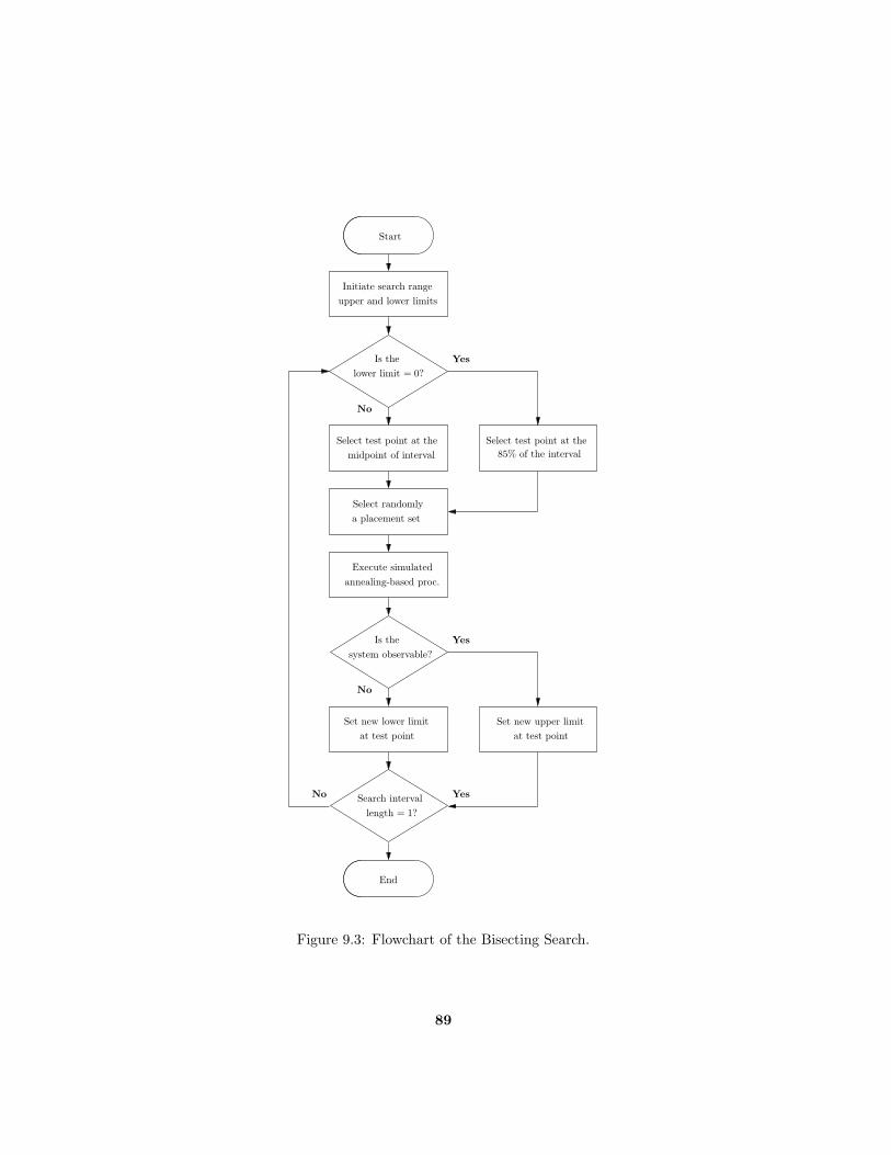
PSfrag replacements
Start
End
Yes
Yes
Yes
No
No
No
Is the
Is the
lower limit = 0?
system observable?
Select test point at the Select test point at the
midpoint of interval 85% of the interval
Set new lower limit Set new upper limit
at test pointat test point
Search interval
length = 1?
Initiate search range
upper and lower limits
Select randomly
a placement set
Execute simulated
annealing-based proc.
Figure 9.3: Flowchart of the Bisecting Search.
89

beginevaluate coverage of PMU placement set SE := N − number of buses in the observed regionT := 15
M := min0.002(
Nνtest
),Mmax
for i := 1 to 40 dofor j := 1 to M do
randomly select a PMUsave the bus location of the selected PMUrandomly select a non-PMU busevaluate coverage of the modified placement setEnew := N − number of buses in the observed regionif Enew = 0 then
return with ‘system observable’and the modified placement set
fi∆E := Enew − Eif ∆E > 0 then
generate a random accept/reject valuewith a probability exp(−∆ET )if reject then
return selected PMU toprevious bus location
fifi
odT := 0.879T
odreturn with ‘system not observable’
end
Figure 9.4: Pseudo-code of the simulated Annealing Algorithm.
90

PSfrag replacements
Start
End
Yes
No Is the
system observable?
Starting bus with PMU
Find bus j which maximizes
the coverage of the network
with the existing PMU’s
Place PMU at bus j
Figure 9.5: Recursive N Security Method.
PSfrag replacements
(a) (b) (c)
AAA
B BB
C CC
DDD
Figure 9.6: Search of alternative placement sets.
PSfrag replacements
A A
BB
C C
D Dpure transit node pure transit node
Figure 9.7: Pure transit node filtering.
91
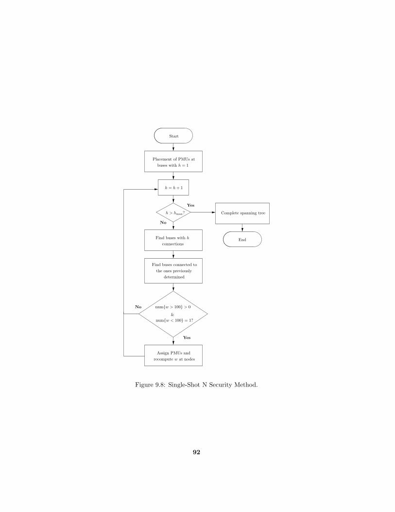
PSfrag replacements
Start
End
Yes
Yes
No
No
Placement of PMUs at
buses with h = 1
h = h+ 1
Complete spanning treeh > hmax?
Find buses with h
connections
Find buses connected to
the ones previously
determined
Assign PMUs and
recompute w at nodes
&
numw > 100 > 0
numw < 100 = 1?
Figure 9.8: Single-Shot N Security Method.
92

9.4 PMU Placement GUI and Settings 93
PSfrag replacements
Start
End
Yes
NoIs the N-1
criterion satisfied?
Starting bus with PMU
Find buses connected
to the current placed PMUs
Find buses connected to
the buses determined in the
previous step
Place PMUs at the
closer buses
Figure 9.9: Recursive N-1 Security Method.
described in Section 9.3.4, whereas the second method is a variant of the algorithmdescribed in Section 9.3.5.
9.4 PMU Placement GUI and Settings
Figure 9.11 depicts the GUI for PMU placement, which allows to select the PMUplacement method and enable to write result in a report file. The listboxes reportthe voltages obtained with the power flow and the ones determined with the linearstatic state estimation based on the current PMU set, as well as the position of thePMUs.
All PMU settings and results are set in the structure PMU. Refer to Appendix Afor details.
9.4.1 Example
An example of report text file of PMU placement is as follows:
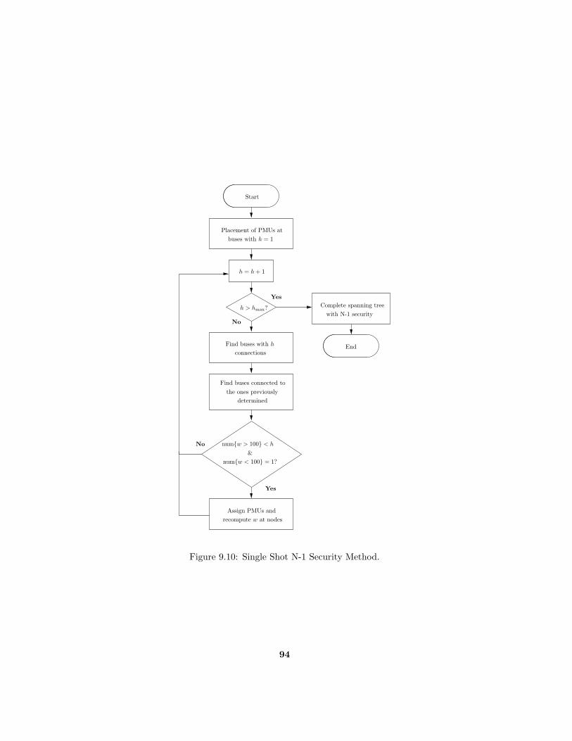
PSfrag replacements
Start
End
Yes
Yes
No
No
Placement of PMUs at
buses with h = 1
h = h+ 1
Complete spanning tree
with N-1 securityh > hmax?
Find buses with h
connections
Find buses connected to
the ones previously
determined
Assign PMUs and
recompute w at nodes
&
numw > 100 < h
numw < 100 = 1?
Figure 9.10: Single Shot N-1 Security Method.
94

9.4 PMU Placement GUI and Settings 95
Figure 9.11: GUI for the PMU placement methods.
PMU PLACEMENT REPORT
P S A T 1.3.0
Author: Federico Milano, (c) 2002-2004
e-mail: [email protected]
website: http://thunderbox.uwaterloo.ca/~fmilano
File: ~/psatd/tests/d_014.mdl
Date: 15-Mar-2004 17:39:21
Placement Method: Annealing Method
Elapsed Time: 0h 0m 0.59293s
STATISTICS
Buses 14
Lines 20
PMUs 3
PMU Sets 1
Meas. Currents 12
Pseudo-Meas. Currents 20
PMU PLACEMENT
Bus Name Set 1
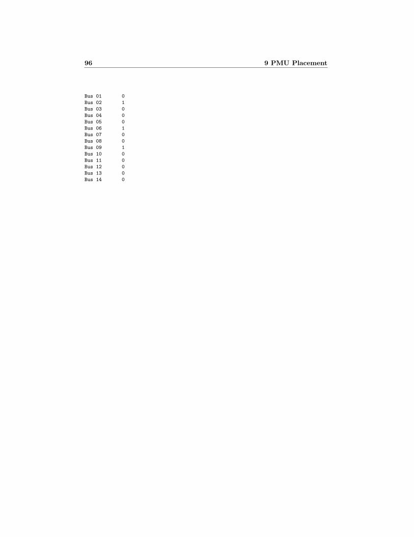
96 9 PMU Placement
Bus 01 0
Bus 02 1
Bus 03 0
Bus 04 0
Bus 05 0
Bus 06 1
Bus 07 0
Bus 08 0
Bus 09 1
Bus 10 0
Bus 11 0
Bus 12 0
Bus 13 0
Bus 14 0

Part III
Models

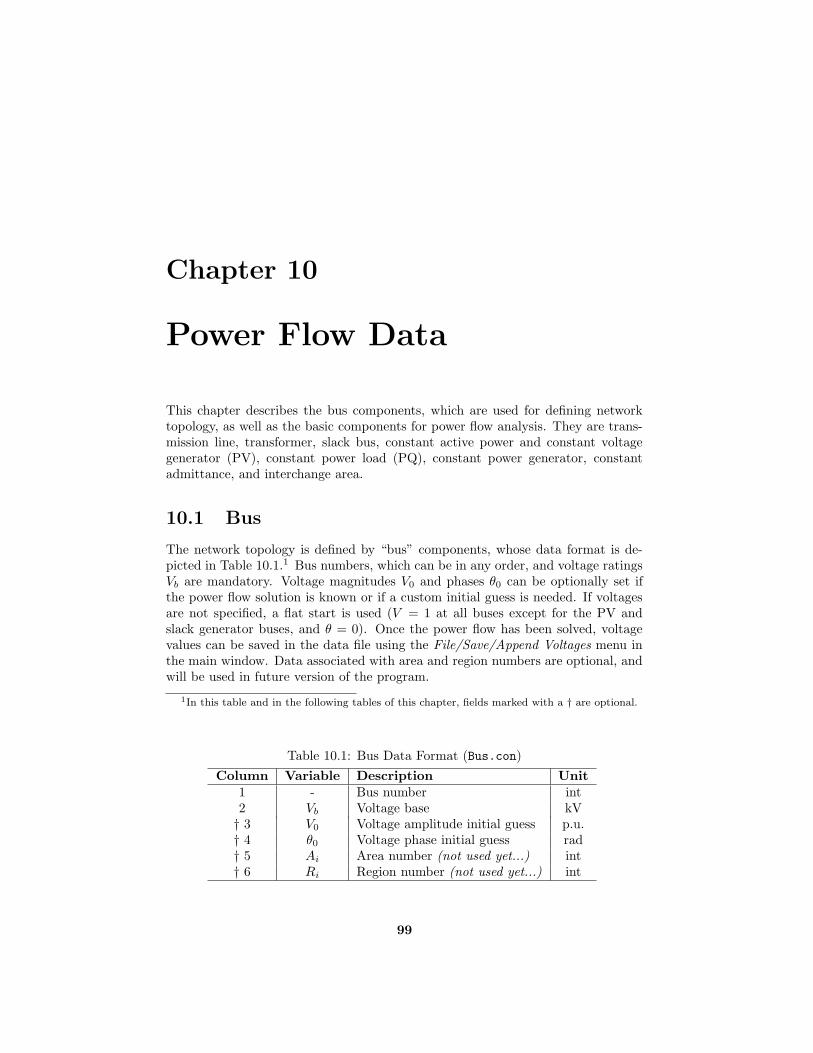
Chapter 10
Power Flow Data
This chapter describes the bus components, which are used for defining networktopology, as well as the basic components for power flow analysis. They are trans-mission line, transformer, slack bus, constant active power and constant voltagegenerator (PV), constant power load (PQ), constant power generator, constantadmittance, and interchange area.
10.1 Bus
The network topology is defined by “bus” components, whose data format is de-picted in Table 10.1.1 Bus numbers, which can be in any order, and voltage ratingsVb are mandatory. Voltage magnitudes V0 and phases θ0 can be optionally set ifthe power flow solution is known or if a custom initial guess is needed. If voltagesare not specified, a flat start is used (V = 1 at all buses except for the PV andslack generator buses, and θ = 0). Once the power flow has been solved, voltagevalues can be saved in the data file using the File/Save/Append Voltages menu inthe main window. Data associated with area and region numbers are optional, andwill be used in future version of the program.
1In this table and in the following tables of this chapter, fields marked with a † are optional.
Table 10.1: Bus Data Format (Bus.con)
Column Variable Description Unit1 - Bus number int2 Vb Voltage base kV† 3 V0 Voltage amplitude initial guess p.u.† 4 θ0 Voltage phase initial guess rad† 5 Ai Area number (not used yet...) int† 6 Ri Region number (not used yet...) int
99

100 10 Power Flow Data
Bus components are defined in the structure Bus, as follows:
1. con: bus data.
2. n: total number of buses.
3. int: bus indexes.
4. Pg: active power injected in the network by generators.
5. Qg: reactive power injected in the network by generators.
6. Pl: active power absorbed from the network by loads.
7. Ql: reactive power absorbed from the network by loads.
8. island: indexes of islanded buses.
The fields Pg, Qg, Pl and Ql are a byproduct of the power flow solution. Inthe fields Pl and Ql shunt power consumptions are not included, since the shuntadmittances are included in the admittance matrix. The field island dependson breaker interventions: if a bus is disconneted from the grid after one or morebreaker interventions, the resulting island is properly handled by the time domainsimulation routine. This means that only buses that would create convergenceproblems are included in the island vector. These are PV generators and PQbuses, since they fix a constant power injection or consumption at the islanded bus.The definition of the island vector is done in the function fm connectivity.
PSAT is component oriented, i.e. standard components can be connected toany bus in any number and type. The only exception is the slack generator (SW)that has to be unique for each bus. Refer to Chapter 22 for a detailed descriptionof component connection rules in PSAT.
10.2 Transmission Line
Fig. 10.1 depicts the circuit used for defining the transmission line lumped model,as described in many power system text books. The line equations are as follows:
Pk = V 2k (gkm + gk0) − VkVm(gkm cos(θk − θm) + bkm sin(θk − θm)) (10.1)
Qk = −V 2k (bkm + bk0) − VkVm(gkm sin(θk − θm) − bkm cos(θk − θm))
Pm = V 2m(gkm + gm0) − VkVm(gkm cos(θk − θm) − bkm sin(θk − θm))
Qm = −V 2m(bkm + bm0) + VkVm(gkm sin(θk − θm) + bkm cos(θk − θm))
Transmission lines are defined in the structure Line, which is used also fortransformers (see Section 10.3). The user can define data in absolute values or inp.u. In the latter case, the length ` of the line has to be ` = 0. If ` 6= 0, it is assumedthat parameters are expressed in unit per km. Table 10.2 depicts the data format oftransmission lines. Imax, Pmax and Smax define the limits for currents, active powerflows and apparent power flows (S =
√P 2 +Q2). These limits are not required in
power flow computations, but can be used for CPF and OPF computations. Referto Chapters 5 and 6 for details.
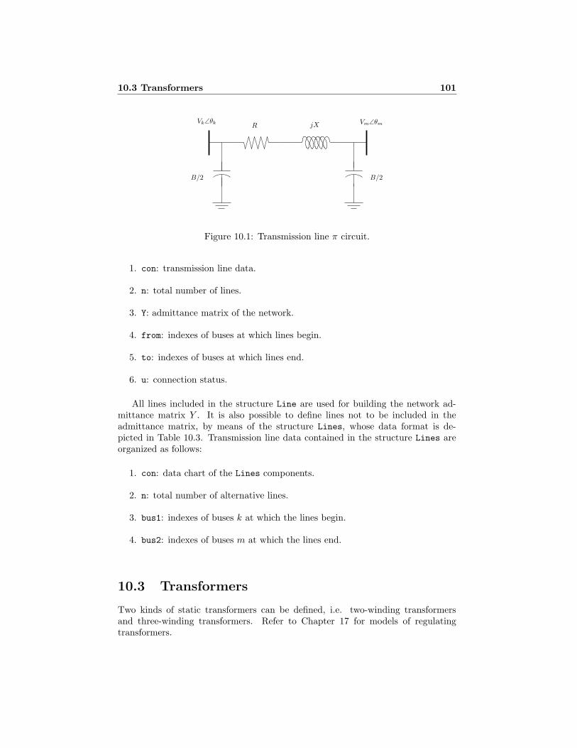
10.3 Transformers 101
PSfrag replacements
R jX
B/2B/2
Vk∠θk Vm∠θm
Figure 10.1: Transmission line π circuit.
1. con: transmission line data.
2. n: total number of lines.
3. Y: admittance matrix of the network.
4. from: indexes of buses at which lines begin.
5. to: indexes of buses at which lines end.
6. u: connection status.
All lines included in the structure Line are used for building the network ad-mittance matrix Y . It is also possible to define lines not to be included in theadmittance matrix, by means of the structure Lines, whose data format is de-picted in Table 10.3. Transmission line data contained in the structure Lines areorganized as follows:
1. con: data chart of the Lines components.
2. n: total number of alternative lines.
3. bus1: indexes of buses k at which the lines begin.
4. bus2: indexes of buses m at which the lines end.
10.3 Transformers
Two kinds of static transformers can be defined, i.e. two-winding transformersand three-winding transformers. Refer to Chapter 17 for models of regulatingtransformers.

Table 10.2: Line Data Format (Line.con)
Column Variable Description Unit1 k From Bus int2 m To Bus int3 Sn Power rating MVA4 Vn Voltage rating kV5 fn Frequency rating Hz6 ` Line length km7 - not used -8 r Resistance p.u. (Ω/km)9 x Reactance p.u. (H/km)10 b Susceptance p.u. (F/km)† 11 - not used -† 12 - not used -† 13 Imax Current limit p.u.† 14 Pmax Active power limit p.u.† 15 Smax Apparent power limit p.u.† 16 u Connection status 0, 1
Table 10.3: Alternative Line Data Format (Lines.con)
Column Variable Description Unit1 k From Bus int2 m To Bus int3 Sn Power rating MVA4 Vn Voltage rating kV5 fn Frequency rating Hz6 r Resistance p.u.7 x Reactance p.u.8 b Susceptance p.u.
102

10.3 Transformers 103
Table 10.4: Transformer Data Format (Line.con)
Column Variable Description Unit1 k From Bus int2 m To Bus int3 Sn Power rating MVA4 Vn Voltage rating kV5 fn Frequency rating Hz6 - not used -7 kT Primary and secondary voltage ratio kV/kV8 r Resistance p.u.9 x Reactance p.u.10 - not used -† 11 a Fixed tap ratio p.u./p.u.† 12 φ Fixed phase shift deg† 13 Imax Current limit p.u.† 14 Pmax Active power limit p.u.† 15 Smax Apparent power limit p.u.† 16 u Connection status 0, 1
10.3.1 Two-Winding Transformers
Two-winding transformers are modeled as series reactances without iron losses andtheir equations are included in (10.1). Table 10.4 depicts the transformer dataformat which is included in the structure Line. The primary and secondary voltageratio kT allows distinguishing between transmission lines and transformers: if kT =0, PSAT takes the component as a line, if kT 6= 0, the component is taken as atransformer. When kT 6= 0, the line length ` is neglected, even if ` 6= 0. The fixedtap ratio a and the fixed phase shift ratio φ are optional parameters.
10.3.2 Three-Winding Transformers
Three-winding transformers are internally modeled as three two-winding transform-ers in a Y connection, as depicted in Fig. 10.2. PSAT processes three-windingtransformer data before running the power flow for the first time and adds one busin the Bus structure and three new lines in the Line structure. Observe that thenew bus will get same voltage rating, area and region as the primary winding bus.
The data format of three-winding transformers allows setting impedances of thetriangle branches, whose relationships with the resulting star impedances are asfollows:
z12 = z1 + z2 (10.2)
z13 = z1 + z3
z23 = z2 + z3

104 10 Power Flow Data
PSfrag replacements
1 1
2 2
3 30
a : 1
z1, Vn1/Vn1
z2, Vn1/Vn2
z3, Vn1/Vn3
z12
z13
z23
Vn1Vn2
Vn3
Figure 10.2: Three-winding transformer equivalent circuit.
Thus, one has:
z1 = (z12 + z13 − z23)/2 (10.3)
z2 = (z12 + z23 − z13)/2
z3 = (z13 + z23 − z12)/2
Three-winding transformers are defined in the structure Twt, which has only the confield. Table 10.5 depicts the three-winding transformer data format. Observe thatPSAT clears the Twt.con matrix after processing it and that there is no functionassociated with three-winding transformer components.
10.4 Slack Generator
Slack generators are modeled as fixed voltage magnitude and phase buses, as follows:
V = V0 (10.4)
θ = θ0
The phase θ0 is assumed to be the reference angle of the system.2 Table 10.6 depictsthe slack generator data, which also contains data used in optimal power flow andcontinuation power flow analysis. In case of distributed slack bus model, the lasttwo parameters P0 and γ are mandatory and the following additional equationholds:
P = −(1 + γkG)P0 (10.5)
where kG is the distributed slack bus variable. If not specified, γ is assumed to beγ = 1. Slack generators are defined in the structure SW, as follows:
1. con: slack generator data.
2. n: total number of slack generators.
3. bus: number of buses to which slack generators are connected.
4. store: copy of the slack generator data. This field is used only in the com-mand line version of PSAT (see Chapter 27).
2Only one slack bus per network can be defined.

Table 10.5: Three-Winding Transformer Data Format (Twt.con)
Column Variable Description Unit1 - Bus number of the 1th winding int2 - Bus number of the 2nd winding int3 - Bus number of the 3rd winding int4 Sn Power rating MVA5 fn Frequency rating Hz6 Vn1 Voltage rating of the 1th winding kV7 Vn2 Voltage rating of the 2nd winding kV8 Vn3 Voltage rating of the 3rd winding kV9 r12 Resistance of the branch 1-2 p.u.10 r13 Resistance of the branch 1-3 p.u.11 r23 Resistance of the branch 2-3 p.u.12 x12 Reactance of the branch 1-2 p.u.13 x13 Reactance of the branch 1-3 p.u.14 x23 Reactance of the branch 2-3 p.u.† 15 a Fixed tap ratio p.u./p.u.† 16 Imax1
Current limit of the 1th winding p.u.† 17 Imax2
Current limit of the 2nd winding p.u.† 18 Imax3
Current limit of the 3rd winding p.u.† 19 Pmax1
Real power limit of the 1th winding p.u.† 20 Pmax2
Real power limit of the 2nd winding p.u.† 21 Pmax3
Real power limit of the 3rd winding p.u.† 22 Smax1
Apparent power limit of the 1th winding p.u.† 23 Smax2
Apparent power limit of the 2nd winding p.u.† 24 Smax3
Apparent power limit of the 3rd winding p.u.† 25 u Connection status 0, 1
Table 10.6: Slack Generator Data Format (SW.con)
Column Variable Description Unit1 - Bus number int2 Sn Power rating MVA3 Vn Voltage rating kV4 V0 Voltage magnitude p.u.5 θ0 Reference Angle p.u.† 6 Qmax Maximum reactive power p.u.† 7 Qmin Minimum reactive power p.u.† 8 Vmax Maximum voltage p.u.† 9 Vmin Minimum voltage p.u.† 10 P0 Active power guess p.u.† 11 γ Loss participation coefficient -
105
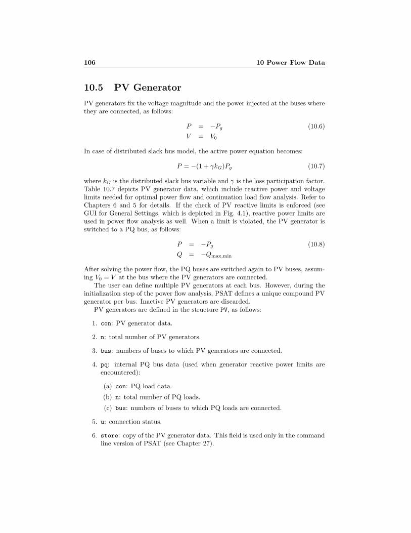
106 10 Power Flow Data
10.5 PV Generator
PV generators fix the voltage magnitude and the power injected at the buses wherethey are connected, as follows:
P = −Pg (10.6)
V = V0
In case of distributed slack bus model, the active power equation becomes:
P = −(1 + γkG)Pg (10.7)
where kG is the distributed slack bus variable and γ is the loss participation factor.Table 10.7 depicts PV generator data, which include reactive power and voltagelimits needed for optimal power flow and continuation load flow analysis. Refer toChapters 6 and 5 for details. If the check of PV reactive limits is enforced (seeGUI for General Settings, which is depicted in Fig. 4.1), reactive power limits areused in power flow analysis as well. When a limit is violated, the PV generator isswitched to a PQ bus, as follows:
P = −Pg (10.8)
Q = −Qmax,min
After solving the power flow, the PQ buses are switched again to PV buses, assum-ing V0 = V at the bus where the PV generators are connected.
The user can define multiple PV generators at each bus. However, during theinitialization step of the power flow analysis, PSAT defines a unique compound PVgenerator per bus. Inactive PV generators are discarded.
PV generators are defined in the structure PV, as follows:
1. con: PV generator data.
2. n: total number of PV generators.
3. bus: numbers of buses to which PV generators are connected.
4. pq: internal PQ bus data (used when generator reactive power limits areencountered):
(a) con: PQ load data.
(b) n: total number of PQ loads.
(c) bus: numbers of buses to which PQ loads are connected.
5. u: connection status.
6. store: copy of the PV generator data. This field is used only in the commandline version of PSAT (see Chapter 27).

10.6 PQ Load 107
Table 10.7: PV Generator Data Format (PV.con)
Column Variable Description Unit1 - Bus number int2 Sn Power rating MVA3 Vn Voltage rating kV4 Pg Active Power p.u.5 V0 Voltage Magnitude p.u.† 6 Qmax Maximum reactive power p.u.† 7 Qmin Minimum reactive power p.u.† 8 Vmax Maximum voltage p.u.† 9 Vmin Minimum voltage p.u.† 10 γ Loss participation coefficient -† 11 u Connection status 0, 1
10.6 PQ Load
PQ loads are modeled as constant active and reactive powers:
P = PL (10.9)
Q = QL
as long as voltages are within the specified limits. If a voltage limit is violated, PQloads are converted into constant impedances, as follows:
P = PV 2/V 2lim (10.10)
Q = QV 2/V 2lim
where Vlim is Vmax or Vmin depending on the case. By default, maximum andminimum voltage limits are assumed to be 1.2 and 0.8 p.u. respectively. Table 10.8depicts the PQ load data format. If z = 0, voltage limit control is disabled.
The user can define multiple PQ loads at each bus. However, during the initial-ization step of the power flow analysis, PSAT defines a unique compound PQ loadper bus. Inactive PQ loads are discarded.
PQ loads can be converted to constant impedances after the power flow solution(see Chapter 4). Refer to Chapter 14 for other static and dynamic load models.
PQ loads are defined in the structure PQ, as follows:
1. con: PQ load data.
2. n: total number of PQ loads.
3. bus: numbers of buses to which PQ loads are connected.
4. gen: 1 if it is a PQ generator, 0 otherwise.
5. P0: initial active power (used with non-conventinal loads of Chapter 14).

108 10 Power Flow Data
Table 10.8: PQ Load Data Format (PQ.con)
Column Variable Description Unit1 - Bus number int2 Sn Power rating MVA3 Vn Voltage rating kV4 PL Active Power p.u.5 QL Reactive Power p.u.† 6 Vmax Maximum voltage p.u.† 7 Vmin Minimum voltage p.u.† 8 z Allow conversion to impedance 0, 1† 9 u Connection status 0, 1
6. Q0: initial reactive power (used with non-conventional loads of Chapter 14).
7. u: connection status.
8. store: copy of the PQ load data. This field is used only in the command lineversion of PSAT (see Chapter 27).
10.7 PQ Generator
PQ generators are modeled as constant active and reactive powers:
P = −Pg (10.11)
Q = −Qg
as long as voltages are within the specified limits. If a voltage limit is violated, PQgenerators are converted into constant impedances, as follows:
P = PV 2/V 2lim (10.12)
Q = QV 2/V 2lim
where Vlim is Vmax or Vmin depending on the case. By default, maximum andminimum voltage limits are assumed to be 1.2 and 0.8 p.u. respectively. Table 10.9depicts the PQ generator data format. If z = 0, voltage limit control is disabled.
Internally, PSAT translates PQ generators into PQ loads with:
PL = −Pg (10.13)
QL = −Qg
The field gen of the PQ structure says if the load was converted from a PQ generator(see Section 10.6). Observe that PQ generators are not converted into constantimpedances after the power flow solution. Observe also that, since PQ generatorsare internally treated as negative PQ loads, it is not allowed connecting a PQ loadat the same bus as a PQ generator.
PQ generators are defined in the structure PQgen, with the only field con.

10.8 Shunt 109
Table 10.9: PQ Generator Data Format (PQgen.con)
Column Variable Description Unit1 - Bus number int2 Sn Power rating MVA3 Vn Voltage rating kV4 Pg Active Power p.u.5 Qg Reactive Power p.u.† 6 Vmax Maximum voltage p.u.† 7 Vmin Minimum voltage p.u.† 8 z Allow conversion to impedance 0, 1
Table 10.10: Shunt Admittance Data Format (Shunt.con)
Column Variable Description Unit1 - Bus number int2 Sn Power rating MVA3 Vn Voltage rating kV4 fn Frequency rating Hz5 g Conductance p.u.6 b Susceptance p.u.† 7 u Connection status 0, 1
10.8 Shunt
Shunt impedances are described by the following equations:
P = gV 2 (10.14)
Q = bV 2
and are included in the network admittance matrix Y . The susceptance b is neg-ative for inductive charges, positive for capacitive ones. Shunts are defined in thestructure Shunt, as follows:
1. con: shunt impedance data.
2. bus: numbers of buses to which shunt are connected.
3. g: column vector of the conductances at each bus of the network.
4. b: column vector of the susceptances at each bus of the network.
5. u: connection status.

110 10 Power Flow Data
Table 10.11: Area Data Format (Areas.con)
Column Variable Description Unit1 - Area number int2 - Slack bus number for the area int3 Sn Power rate MVA4 Pex Area interchange export (> 0 = out) p.u.5 Ptol Area interchange tolerance p.u.
10.9 Area
Interchange area data can be defined in the current version of PSAT, although theyare not used in any routine. Each area is defined by a unique number, which hasto correspond to one of the numbers defined in the column 5 of the Bus.con data.
A slack bus must be defined for each area. This slack bus is just a “suggestion”and does not affect or redefine the SW.con data. However, observe that the slackbuses that are defined in the SW.con data should be consistent with the slack busesdefined in the interchange area data. Interchange areas are defined in the classAreas, as follows:
1. con: area data.
2. n: number or areas.
3. slack: indexes of slack buses for each area.

Chapter 11
CPF and OPF Data
This section describes the components needed for the OPF routines. The basiccomponents are the slack generator, the PV generator and the PQ load. As definedin Tables 10.6, 10.7 and 10.8, the user can define the reactive power and voltagelimits for the generation, and the voltage limits for the loads. Furthermore, in thedefinition of transmission lines and transformers, it is possible to set a limit fora maximum flow (current, active power or apparent power). Then, in the OPFwindow, the flow type can be specified and selected in a popup menu.
For the voltages at all the N network buses, one has:
Vmini≤ Vi ≤ Vmaxi
i = 1, . . . , N (11.1)
whereas the limits for the generation are the following:
Qmini≤ Qgi
≤ Qmaxii = 1, . . . , Ng (11.2)
where Ng is the total number of generators given by the sum of the slack and PVgenerators. Finally the flows constraints are:
Φi ≤ Φmaxii = 1, . . . , NL (11.3)
If no constraint is defined for lines or transformers, i.e. the 13th, 14th or 15th
element is left blank or set to zero in the Line.con chart, a “huge” limit for theflow is used.
The components SW, PV , PQ and Line allow to define only some security limits.The cost parameters and additional market constraints are defined in other struc-tures, described below, that are specifically used for the OPF routines. For thegeneration three structures can be defined:
1. Supply: power bids, generator power directions and limits.
2. Rsrv: power reserve data.
3. Rmpg: power ramping data.
111
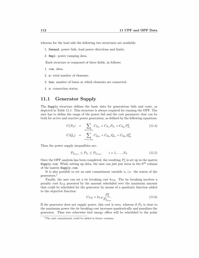
112 11 CPF and OPF Data
whereas for the load side the following two structures are available:
1. Demand: power bids, load power directions and limits.
2. Rmpl: power ramping data.
Each structure is composed of three fields, as follows:
1. con: data.
2. n: total number of elements.
3. bus: number of buses at which elements are connected.
4. u: connection status.
11.1 Generator Supply
The Supply structure defines the basic data for generations bids and costs, asdepicted in Table 11.1. This structure is always required for running the OPF. Theuser has to define the range of the power bid and the cost parameter that can beboth for active and reactive power generation, as defined by the following equations:
C(PS) =∑
i=1,NS
CP0i+ CP1i
PSi+ CP2i
P 2Si
(11.4)
C(Qg) =∑
i=1,NS
CQ0i+ CQ1i
Qgi+ CQ2i
Q2gi
Then the power supply inequalities are:
PSmin i≤ PSi
≤ PSmax ii = 1, . . . , NS (11.5)
Once the OPF analysis has been completed, the resulting P ∗S is set up in the matrix
Supply.con. While setting up data, the user can just put zeros in the 6th columnof the matrix Supply.con.
It is also possible to set an unit commitment variable u, i.e. the status of thegenerators.1
Finally, the user can set a tie breaking cost kTB . The tie breaking involves apenalty cost kTB prorated by the amount scheduled over the maximum amountthat could be scheduled for the generator by means of a quadratic function addedto the objective function:
CTB = kTBP 2
S
PSmax
(11.6)
If the generator does not supply power, this cost is zero, whereas if PS is close tothe maximum power the tie breaking cost increases quadratically and penalizes thegenerator. Thus two otherwise tied energy offers will be scheduled to the point
1The unit commitment could be added in future versions.
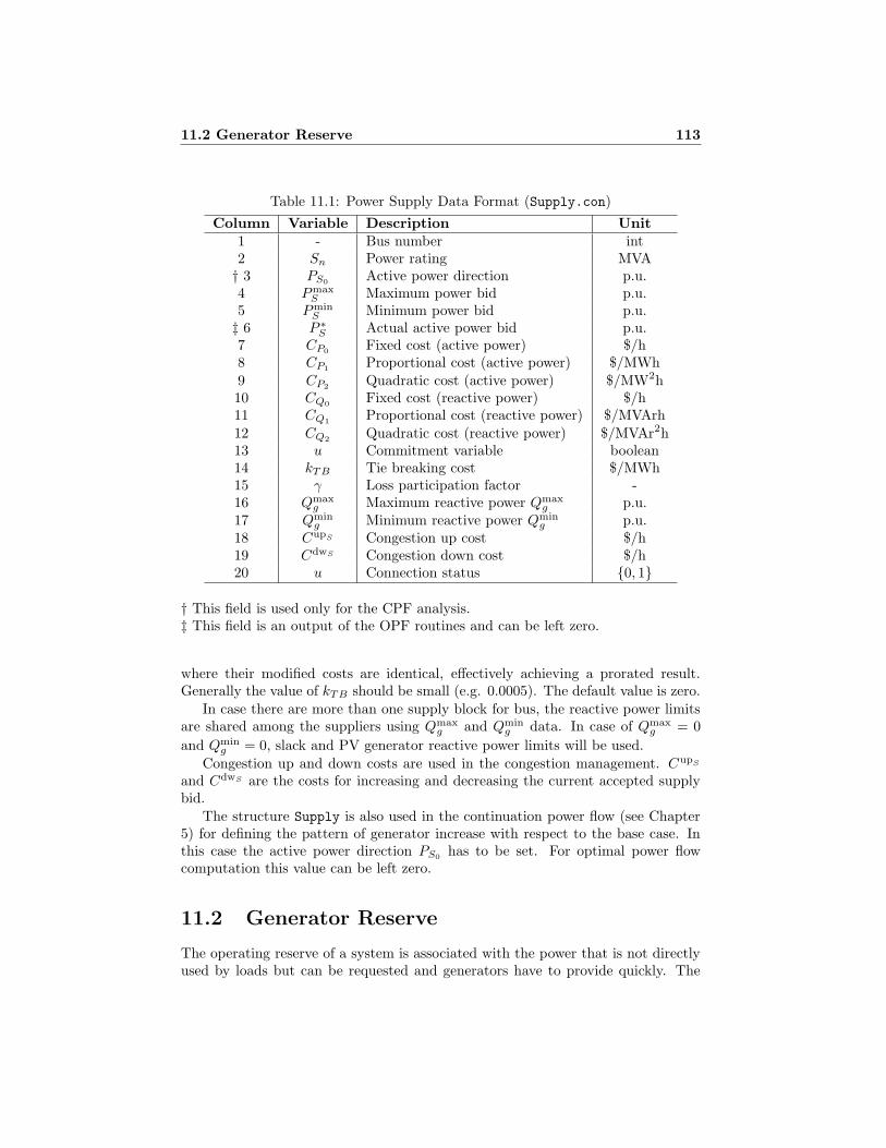
11.2 Generator Reserve 113
Table 11.1: Power Supply Data Format (Supply.con)
Column Variable Description Unit1 - Bus number int2 Sn Power rating MVA† 3 PS0
Active power direction p.u.4 Pmax
S Maximum power bid p.u.5 Pmin
S Minimum power bid p.u.‡ 6 P ∗
S Actual active power bid p.u.7 CP0
Fixed cost (active power) $/h8 CP1
Proportional cost (active power) $/MWh9 CP2
Quadratic cost (active power) $/MW2h10 CQ0
Fixed cost (reactive power) $/h11 CQ1
Proportional cost (reactive power) $/MVArh12 CQ2
Quadratic cost (reactive power) $/MVAr2h13 u Commitment variable boolean14 kTB Tie breaking cost $/MWh15 γ Loss participation factor -16 Qmax
g Maximum reactive power Qmaxg p.u.
17 Qming Minimum reactive power Qmin
g p.u.18 CupS Congestion up cost $/h19 CdwS Congestion down cost $/h20 u Connection status 0, 1
† This field is used only for the CPF analysis.‡ This field is an output of the OPF routines and can be left zero.
where their modified costs are identical, effectively achieving a prorated result.Generally the value of kTB should be small (e.g. 0.0005). The default value is zero.
In case there are more than one supply block for bus, the reactive power limitsare shared among the suppliers using Qmax
g and Qming data. In case of Qmax
g = 0
and Qming = 0, slack and PV generator reactive power limits will be used.
Congestion up and down costs are used in the congestion management. CupS
and CdwS are the costs for increasing and decreasing the current accepted supplybid.
The structure Supply is also used in the continuation power flow (see Chapter5) for defining the pattern of generator increase with respect to the base case. Inthis case the active power direction PS0
has to be set. For optimal power flowcomputation this value can be left zero.
11.2 Generator Reserve
The operating reserve of a system is associated with the power that is not directlyused by loads but can be requested and generators have to provide quickly. The
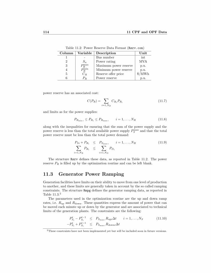
114 11 CPF and OPF Data
Table 11.2: Power Reserve Data Format (Rsrv.con)
Column Variable Description Unit1 - Bus number int2 Sn Power rating MVA3 Pmax
R Maximum power reserve p.u.4 Pmin
R Minimum power reserve p.u.5 CR Reserve offer price $/MWh6 PR Power reserve p.u.
power reserve has an associated cost:
C(PR) =∑
i=1,NR
CRiPRi
(11.7)
and limits as for the power supplies:
PRmin i≤ PRi
≤ PRmax ii = 1, . . . , NR (11.8)
along with the inequalities for ensuring that the sum of the power supply and thepower reserve is less than the total available power supply Pmax
S and that the totalpower reserve must be less than the total power demand:
PSi + PRi≤ PSmax i
i = 1, . . . , NR (11.9)∑
i=1,NR
PRi≤
∑
i+1,ND
PDi
The structure Rsrv defines these data, as reported in Table 11.2. The powerreserve PR is filled up by the optimization routine and can be left blank.
11.3 Generator Power Ramping
Generation facilities have limits on their ability to move from one level of productionto another, and these limits are generally taken in account by the so called rampingconstraints. The structure Rmpg defines the generator ramping data, as reported inTable 11.3.2
The parameters used in the optimization routine are the up and down ramprates, i.e. Rup and Rdown. These quantities express the amount of power that canbe moved each minute up or down by the generator and are associated to technicallimits of the generation plants. The constraints are the following:
P tSi
− P t−1Si
≤ PSmax iRupi∆t i = 1, . . . , NS (11.10)
−P tSi
+ P t−1Si
≤ PSmax iRdowni∆t
2These constraints have not been implemented yet but will be included soon in future versions.

11.4 Load Demand 115
Table 11.3: Generator Power Ramping Data Format (Rmpg.con)
Column Variable Description Unit1 - Supply number int2 Sn Power rating MVA3 Rup Ramp rate up p.u./h4 Rdown Ramp rate down p.u./h5 UT Minimum # of period up h6 DT Minimum # of period down h7 UTi Initial # of period up int8 DTi Initial # of period down int9 CSU Start up cost $
Along with these ramp limits, the user can define also a maximum reserve ramprate RRmax
, that multiplied by the time interval ∆t, expresses the maximum amountof power that can be dedicated to the reserve, thus:
PRi≤ RRmax i
∆t i = 1, . . . , NR (11.11)
If the generator output is low, also the operating reserve can decrease, and theoperating reserve loading point PRLP allows to reduce the power reserve for lowoutputs:
PRi≤ PSi
RRmax i∆t
PRLPi
i = 1, . . . , NR (11.12)
Thus, the power reserve PR will be the minimum between (11.11) and (11.12).
11.4 Load Demand
The Demand structure defines the basic data for load demand bids and costs, aspresented in Table 11.4. The user has to define the maximum and minimum powerbids, as well as the cost coefficients that can be both for active and reactive powers.The cost functions, similar to (11.4) for the power supplies, are:
C1(PD) =∑
i=1,ND
CP0i+ CP1i
PDi+ CP2i
P 2Di
(11.13)
C2(PD) =∑
i=1,ND
CQ0i+ CQ1i
PDitan(φi) + CQ2i
P 2Di
tan(φi)2
where
tanφi =QD0i
PD0i
(11.14)
As for the constraints, one has:
PRmin i≤ PRi
≤ PRmax ii = 1, . . . , NR (11.15)

116 11 CPF and OPF Data
The power factor angle φ is used for computing reactive power costs. The powerfactor angle is obtained using power directions PD0
and QD0. Observe that, their
ratio can be different from the power factor of the base case load defined in the PQ
structure .
Once the OPF analysis has been completed, the resulting P ∗D is set up in the
matrix Demand.con. While setting up data, the user can just put zeros in the 7th
column of the matrix Demand.con.
It possible to set an unit commitment variable, i.e. the status of the loads.3
Finally, the user can set a tie breaking cost kTB . The tie breaking involves apenalty cost kTB prorated by the amount scheduled over the maximum amountthat could be scheduled for the load by means of a quadratic function added to theobjective function:
CTB = kTBP 2
D
PDmax
(11.16)
If the load does not consume power, this cost is zero, whereas if PD is close tothe maximum power the tie breaking cost increases quadratically and penalizes theload. Thus two otherwise tied energy demands will be scheduled to the point wheretheir modified costs are identical, effectively achieving a prorated result. Generallythe value of kTB should be small (e.g. 0.0005). The default value is zero.
Congestion up and doen costs are used in the congestion management. CupD
and CdwD are the costs for increasing and decreasing the current accepted demandbid.
The structure Demand is also used in the continuation load flow (see Chapter5) for defining the pattern of load increase with respect to the base case. TheCPF routine uses PD0
and QD0to define the active and reactive power directions,
respectively.
11.5 Demand Profile
The structure Ypdp defines the demand profile for multiperiod market clearingmodels.4 The user can input data using two different formats, namely free formatand yearly profile.
The free format is simply a vector (of any length 6= 206) of numbers representingthe percentage of power demand for the period t. Each element of the vector definesa period t, and the whole vector length represent the time horizon of the marketclearing model. For example:
Ypdp.con = [80 90 100 110 100];
defines 5 time periods, for which the percentage ξt of the demand is 80, 90, 100,110 and 100%, respectively. The percentage multiplies the base case powers PL0 (if
3The unit commitment could be added in future versions.4Multiperiod market clearing models are currently available only for the PSAT-GAMS inter-
face.
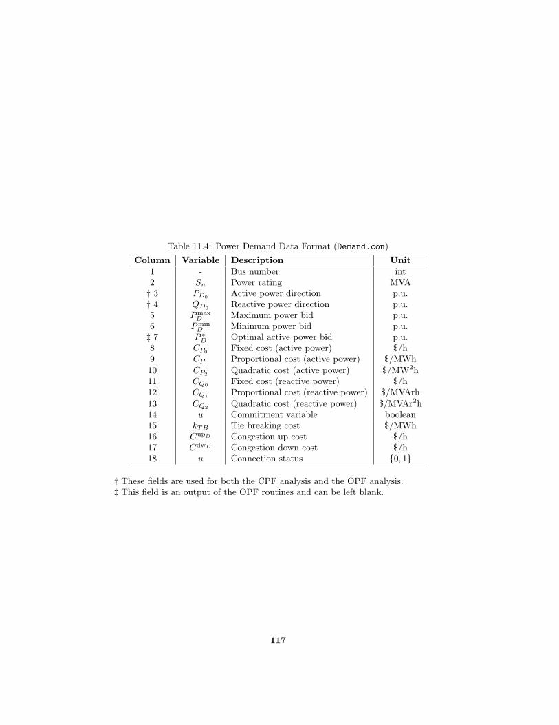
Table 11.4: Power Demand Data Format (Demand.con)
Column Variable Description Unit1 - Bus number int2 Sn Power rating MVA† 3 PD0
Active power direction p.u.† 4 QD0
Reactive power direction p.u.5 Pmax
D Maximum power bid p.u.6 Pmin
D Minimum power bid p.u.‡ 7 P ∗
D Optimal active power bid p.u.8 CP0
Fixed cost (active power) $/h9 CP1
Proportional cost (active power) $/MWh10 CP2
Quadratic cost (active power) $/MW2h11 CQ0
Fixed cost (reactive power) $/h12 CQ1
Proportional cost (reactive power) $/MVArh13 CQ2
Quadratic cost (reactive power) $/MVAr2h14 u Commitment variable boolean15 kTB Tie breaking cost $/MWh16 CupD Congestion up cost $/h17 CdwD Congestion down cost $/h18 u Connection status 0, 1
† These fields are used for both the CPF analysis and the OPF analysis.‡ This field is an output of the OPF routines and can be left blank.
117

118 11 CPF and OPF Data
used) and demand bid limits PDmaxand PDmin
, so that:
PL0(t) =ξt
100PL0 ∀t ∈ T (11.17)
PDmax(t) =
ξt
100PDmax
∀t ∈ T (11.18)
PDmin(t) =
ξt
100PDmin
∀t ∈ T (11.19)
where T = 1, 2, 3, 4, 5 for this example.The yearly demand profile is used to define a database for a one day long time
horizon (T = 24 hours). The user can tune the coefficients by chosing the the seasonand the day of the week. Thus, the 24 coefficients ξt are computed as follows:
ξt =kt
α(α)
100· kβ(β)
100· kγ(γ)
100100 (11.20)
where ktα (24 elements), kβ (scalar) and kγ (scalar) are in % and represent the kind
of the day, the day of the week and the week of the year, respectively, and theindexes α, β and γ are as follows:
α: index of the kind of the day in the range from 1 to 6, with the followingnotation:
1: winter working day
2: winter weekend
3: summer working day
4: summer weekend
5: spring/fall working day
6: spring/fall weekend
β: day of the week in the range from 1 (Monday) to 7 (Sunday).
γ: week of the year in the range from 1 to 52.
11.6 Load Ramping
Although less commonly used than the generation ramp rate, it is possible to defineload ramp rates. These take in account the load ability to move from one level ofconsumption to another. The structure Rmpl defines the load ramping data, asreported in Table 11.6.5
The parameters used in the optimization routine are the up and down ramprates, i.e. Rup and Rdown. These quantities express the amount of power that can
5These constraints have not been implemented yet but will be included in future versions.

Table 11.5: Demand Profile Data Format (Ypdp.con)
Column Variable Description Unit1-24 kt
α(1) Daily profile for a winter working day %25-48 kt
α(2) Daily profile for a winter weekend %49-72 kt
α(3) Daily profile for a summer working day %73-96 kt
α(4) Daily profile for a summer weekend %97-127 kt
α(5) Daily profile for a spring/fall working day %121-144 kt
α(6) Daily profile for a spring/fall weekend %145-151 kβ Profile for the days of the week %152-203 kγ Profile for the weeks of the year %
204 α Kind of the day 1, . . . , 6205 β Day of the week 1, . . . , 7206 γ Week of the year 1, . . . , 52
PSfrag replacements
55
65
75
85
95
105
60
70
80
90
100
2 4 6 8 10 12 14 16 18 20 22 24
hour
dem
and
pro
file
%
Figure 11.1: Example of daily demand profile.
119

120 11 CPF and OPF Data
Table 11.6: Load Ramping Data Format (Rmpl.con)
Column Variable Description Unit1 - Bus number int2 Sn Power rating MVA3 Rup Ramp rate up p.u./min4 Rdown Ramp rate down p.u./min
be moved each minute up or down by the load and are associated to technical limitsin load facilities as follows:
P tDi
− P t−1Di
≤ PDmax iRupi∆t i = 1, . . . , ND (11.21)
−P tDi
+ P t−1Di
≤ PDmax iRdowni∆t
These equations are conceptually similar to (11.10) for the generation ramp rate,and uses the same time interval ∆t defined in the OPF window.

Chapter 12
Faults & Breakers
This chapter describes symmetrical three phase faults and breakers.
12.1 Fault
Table 12.1 depicts data for three phase faults, i.e. the time tf of occurrence of thefault, the clearance time tc and the internal impedance of the fault rf and xf .
During time domain simulations, a time vector for computing a point slightlybefore and slightly after the fault occurrences is created. When the faults or thefault clearances occur, the shunt admittances of the network are modified and theadmittance matrix is recomputed.
Three phase faults are defined in the Fault structure, as follows:
1. con: Fault data.
2. n: total number of faults.
3. bus: vector of bus numbers to which faults are connected.
4. dat: internal data.
5. V: vector of pre-fault voltages.
6. ang: vector of pre-fault angles.
7. delta: mean of synchronous machine rotor angles.
12.2 Breaker
Table 12.2 depicts the data format for transmission line breakers. Besides MVA,kV and Hz ratings, the user can set up two intervention times and a status for thebreaker.
121
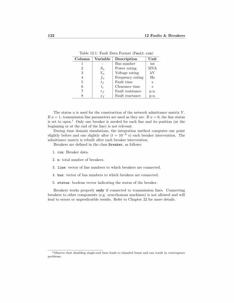
122 12 Faults & Breakers
Table 12.1: Fault Data Format (Fault.con)
Column Variable Description Unit1 - Bus number int2 Sn Power rating MVA3 Vn Voltage rating kV4 fn Frequency rating Hz5 tf Fault time s6 tc Clearance time s7 rf Fault resistance p.u.8 xf Fault reactance p.u.
The status u is used for the construction of the network admittance matrix Y .If u = 1, transmission line parameters are used as they are. If u = 0, the line statusis set to open.1 Only one breaker is needed for each line and its position (at thebeginning or at the end of the line) is not relevant.
During time domain simulations, the integration method computes one pointslightly before and one slightly after (t = 10−6 s) each breaker intervention. Theadmittance matrix is rebuilt after each breaker intervention.
Breakers are defined in the class Breaker, as follows:
1. con: Breaker data.
2. n: total number of breakers.
3. line: vector of line numbers to which breakers are connected.
4. bus: vector of bus numbers to which breakers are connected.
5. status: boolean vector indicating the status of the breaker.
Breakers works properly only if connected to transmission lines. Connectingbreakers to other components (e.g. syncrhonous machines) is not allowed and willlead to errors or unpredicatble results. Refer to Chapter 22 for more details.
1Observe that disabling single-end lines leads to islanded buses and can result in convergenceproblems.

Table 12.2: Breaker Data Format (Breaker.con)
Column Variable Description Unit1 - Line number int2 - Bus number int3 Sn Power rating MVA4 Vn Voltage rating kV5 fn Frequency rating Hz6 u Connection status 0, 17 t1 First intervention time s8 t2 Second intervention time s
123


Chapter 13
Measurements
This chapter describes components intended for measurements of non-standardquantities during time domain simulations. Measurement devices currently imple-mented in PSAT are the bus frequency measurement and the Phasor MeasurementUnit (PMU).
13.1 Bus Frequency Measurement
The bus frequency measurement is obtained by means of a high-pass and a low-passfilter, as depicted in Fig. 13.1. Differential equations are as follows:
x =1
Tf
( 1
2πf0
1
Tf(θ − θ0) − x
)(13.1)
ω = (∆ω + 1 − ω)/Tω
where ∆ω is:
∆ω = −x+1
2πf0
1
Tf(θ − θ0) (13.2)
Bus frequency measurement data are stored in the structure Busfreq, with thefollowing fields:
1. con: Bus frequency measurement data.
PSfrag replacements
∆ω ω
ωn = 1
θ
θ0
11 s +
+
+
−2πf0 1 + sTf 1 + sTω
Figure 13.1: Bus frequency measurement filter.
125

126 13 Measurements
Table 13.1: Bus Frequency Measurement Data Format (Busfreq.con)
Column Variable Description Unit1 - Bus number int2 Tf Time constant of the high-pass filter s3 Tω Time constant of the low-pass filter s
2. n: total number of components.
3. dat: Bus frequency measurement parameters.
4. x: indexes of state variables x.
5. w: indexes of state variables ω.
Table 13.1 depicts the data format for the bus frequency measurement compo-nents.
13.2 Phasor Measurement Unit (PMU)
A Phasor Measurement Unit (PMU) is a device able to measure the magnitude andthe angle of a phasor. Basic concepts, definitions and applications about PMUs canbe found in [Working Group H-7 of the Relaying Channels Subcommittee of theIEEE Power System Relaying Committee 1994].
Let define a sinusoidal quantity:
x(t) = XM cos(ωt+ φ) (13.3)
its phasor representation is:
X =XM√
2ejφ (13.4)
The phasor is defined for a pure constant sinusoid, but it can also be used fortransients, assuming that the phasor is the fundamental frequency component of awaveform over a finite interval (observation window).
PMUs works on sampled measures (see Fig. 13.2). In the case of x(t), we candefine the samples signal xk at t = kτ , where τ is the sampling interval. Using aDiscrete Fourier Transform (DFT), the phasor X is given by:
X =1√2
2
N(Xc − jXs) (13.5)
where N is the number of samples in one period of the nominal fundamental fre-

13.2 Phasor Measurement Unit 127
PSfrag replacements
1
2
N
N + 1
Figure 13.2: Phasors from sample data.
quency f0, and:
Xc =N∑
k=1
xk cos kθ (13.6)
Xs =
N∑
k=1
xk sin kθ (13.7)
and θ is the sampling angle associated with the sampling interval τ , as follows:
θ =2π
N= 2πf0τ (13.8)
A typical sampling rate in many relaying and measurements functions is 12 timesthe power system frequency (e.g. 720 Hz for a 60 Hz power system).
Equation (13.5) represents a non-recursive DFT calculation. A recursive cal-culation is an efficient method for time varying phasors. Let Xr be the phasorcorresponding to the data set xk = r, r + 1, . . . , N + r − 1, and let a new datasample be obtained to produce a new data set xk = r + 1, r + 2, . . . , N + r. Therecursive phasor corresponding to the new data window Xr+1 is as follows:
Xr+1 = Xr +1√2
2
N(xN+r − xr)e
−jrθ (13.9)
A recursive calculation through a moving window data sample is faster than a non-recursive one, needs only two sample data at each calculation (xN+r and xr) andprovides a stationary phasor.
If the quantity x(t) undergoes a transient, the moving window detects the am-plitude and angle variations with a delay which depends on the time sample rate

128 13 Measurements
Table 13.2: Phasor Measurement Unit Data Format (Pmu.con)
Column Variable Description Unit1 - Bus number int2 Vn Voltage rate kV3 fn Frequency rate Hz4 Tv Voltage magnitude time constant s5 Tθ Voltage phase time constant s
τ . If the system frequency f0 undergoes a variation ∆f , the positive sequence ofthe phasor undergoes the following change, at each rth time sampling:
Xr(f0 + ∆f) = Xe−j(N−1)π∆f∆t sin(N∆f∆t)
N sin(∆f∆t)ej2πr∆f∆t (13.10)
thus, the rate of change of the phasor angle is as follows:
dψ
dt= 2π∆f (13.11)
The PMU model implemented in PSAT is used for bus voltage magnitude andphase measurements. The measurement is modeled as a simple low pass filter, asfollows:
vm = (V − vm)/Tm (13.12)
θm = (θ − θm)/Tθ (13.13)
where V and θ are the voltage magnitude and phase, respectively.PMU data are stored in the structure Pmu,1 with the following fields:
1. con: PMU data.
2. n: total number of components.
3. dat: PMU parameters.
4. vm: indexes of state variables vm.
5. thetam: indexes of state variables θm.
Table 13.2 depicts the data format for the PMU components.
1Do not confuse the structure Pmu for PMU devices models with the structure PMU which isused in the PMU placement algorithms illustrated in Chapter 9.

Chapter 14
Loads
This chapter describes static and dynamic nonlinear loads. They are voltage depen-dent load, ZIP load, frequency dependent load, exponential recovery load, thermo-statically controlled load,, Jimma’s load , and mixed load. These models requiresa PQ load in order to initialize parameters and state variables. Voltage dependentand ZIP loads can be optionally included in the power flow analysis.
14.1 Voltage Dependent Load
Voltage dependent loads (VDL) are loads whose powers are monomial functions ofthe bus voltage, as follows:
P = P0(V/V0)αP (14.1)
Q = Q0(V/V0)αQ
where V0 is the initial voltage at the load bus as obtained by the power flow solution.Other parameters are defined in Table 14.1, which depicts the VDL data format.
VDLs can also be included directly in the power flow analysis. In this case, theinital voltage is not known V0, thus the following equations will be used:
P = P0VαP (14.2)
Q = Q0VαQ
The units of P0 and Q0 depends on the parameter z. If z = 1, the VDL is initializedafter the power flow analysis, and P0 and Q0 are in percentage of the PQ load powerconnected at the VDL bus. Observe that if z = 1, it is mandatory to connect a PQload at the VDL bus. If u = 0, the VDL is included in the power flow analysis, andP0 and Q0 are in p.u. In this case it is not necessary to connect a PQ load at theVDL bus.
Observe that equations (14.1) are a simplification of the nonlinear general ex-ponential voltage frequency dependent load described in Section 14.3.
Voltage dependent loads are defined in the structure Mn, as follows:
129

130 14 Loads
Table 14.1: Voltage Dependent Load Data Format (Mn.con)
Column Variable Description Unit1 - Bus number int2 Sn Power rating MVA3 Vn Voltage rating kV4 P0 Active power rating % (p.u.)5 Q0 Reactive power rating % (p.u.)6 αP Active power exponent -7 αQ Reactive power exponent -8 z Initialize after power flow 1, 09 u Connection status 1, 0
1. con: voltage dependent load data.
2. n: total number of voltage dependent loads.
3. bus: numbers of buses to which voltage dependent loads are connected.
4. init: status for power flow computations.
5. u: connection status.
6. store: copy of the voltage dependent load data. This field is used only inthe command line version of PSAT (see Chapter 27).
If the option for changing the constant power loads into constant impedance isenabled, PQ loads are redefined as monomial loads and added to the structure Mn.In this case it is assumed that αP = αQ = 2 and
P0 = PL/V20 (14.3)
Q0 = QL/V20
where V0 is the voltage value obtained with the power flow solution.
14.2 ZIP Load
The polynomial or ZIP loads are loads whose powers are a quadratix expression ofthe bus voltage, as follows:
P = g(V/V0)2 + IP (V/V0) + Pn (14.4)
Q = b(V/V0)2 + IQ(V/V0) +Qn
where V0 is the initial voltage at the load bus as obtained by the power flow solution.Other parameters are defined in Table 14.2, which depicts the ZIP load data format.
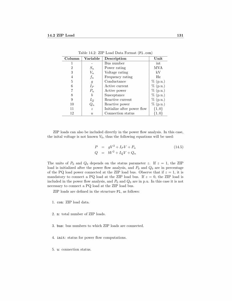
14.2 ZIP Load 131
Table 14.2: ZIP Load Data Format (Pl.con)
Column Variable Description Unit1 - Bus number int2 Sn Power rating MVA3 Vn Voltage rating kV4 fn Frequency rating Hz5 g Conductance % (p.u.)6 IP Active current % (p.u.)7 Pn Active power % (p.u.)8 b Susceptance % (p.u.)9 IQ Reactive current % (p.u.)10 Qn Reactive power % (p.u.)11 z Initialize after power flow 1, 012 u Connection status 1, 0
ZIP loads can also be included directly in the power flow analysis. In this case,the inital voltage is not known V0, thus the following equations will be used:
P = gV 2 + IPV + Pn (14.5)
Q = bV 2 + IQV +Qn
The units of P0 and Q0 depends on the status parameter z. If z = 1, the ZIPload is initialized after the power flow analysis, and P0 and Q0 are in percentageof the PQ load power connected at the ZIP load bus. Observe that if z = 1, it ismandatory to connect a PQ load at the ZIP load bus. If z = 0, the ZIP load isincluded in the power flow analysis, and P0 and Q0 are in p.u. In this case it is notnecessary to connect a PQ load at the ZIP load bus.
ZIP loads are defined in the structure Pl, as follows:
1. con: ZIP load data.
2. n: total number of ZIP loads.
3. bus: bus numbers to which ZIP loads are connected.
4. init: status for power flow computations.
5. u: connection status.

132 14 LoadsPSfrag replacements
∆ωθ
θ0
1 s+
−2πf0 1 + sTF
Figure 14.1: Measure of frequency deviation.
14.3 Frequency Dependent Load
A generalized exponential voltage frequency dependent load is modeled as fol-lows [Hirsch 1994]:
P =kP
100
( VV0
)αP
(1 + ∆ω)βP (14.6)
Q =kQ
100
( VV0
)αQ
(1 + ∆ω)βQ
where ∆ω represents the frequency deviation at the load bus, determined by filteringand differentiating the bus voltage phase angle θ as follows (see Fig. 14.1):
x = − 1
TF
( 1
2πf0
1
TF(θ − θ0) + x
)(14.7)
∆ω = x+1
2πf0
1
TF(θ − θ0)
and V0 and θ0 are the voltage magnitude and phase angle determined in the powerflow solution. This component is initialized after power flow computations. APQ load must be connected to the same bus, and its power and voltage ratingswill be inherited by the frequency dependent load. Table 14.3 reports the dataformat for the component whereas Table 14.4 depicts some typical coefficients forcharacteristic loads [Berg 1973].
Frequency dependent loads are defined in the structure Fl, as follows:
1. con: frequency dependent load data.
2. n: total number of polynomial power loads.
3. bus: bus numbers to which frequency dependent loads are connected.
4. a0: initial bus voltage phase angles.
5. Dw: bus frequency deviations ∆ω.
6. x: indexes of filter state variables x.
7. u: connection status.
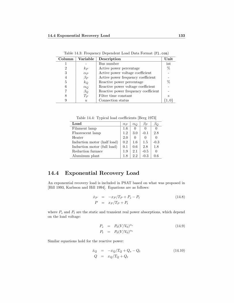
14.4 Exponential Recovery Load 133
Table 14.3: Frequency Dependent Load Data Format (Fl.con)
Column Variable Description Unit1 - Bus number int2 kP Active power percentage %3 αP Active power voltage coefficient -4 βP Active power frequency coefficient -5 kQ Reactive power percentage %6 αQ Reactive power voltage coefficient -7 βQ Reactive power frequency coefficient -8 TF Filter time constant s9 u Connection status 1, 0
Table 14.4: Typical load coefficients [Berg 1973]
Load αP αQ βP βQ
Filament lamp 1.6 0 0 0Fluorescent lamp 1.2 3.0 -0.1 2.8Heater 2.0 0 0 0Induction motor (half load) 0.2 1.6 1.5 -0.3Induction motor (full load) 0.1 0.6 2.8 1.8Reduction furnace 1.9 2.1 -0.5 0Aluminum plant 1.8 2.2 -0.3 0.6
14.4 Exponential Recovery Load
An exponential recovery load is included in PSAT based on what was proposed in[Hill 1993, Karlsson and Hill 1994]. Equations are as follows:
xP = −xP /TP + Ps − Pt (14.8)
P = xP /TP + Pt
where Ps and Pt are the static and transient real power absorptions, which dependon the load voltage:
Ps = P0(V/V0)αs (14.9)
Pt = P0(V/V0)αt
Similar equations hold for the reactive power:
xQ = −xQ/TQ +Qs −Qt (14.10)
Q = xQ/TQ +Qt

134 14 Loads
Table 14.5: Exponential Recovery Load Data Format (Exload.con)
Column Variable Description Unit1 - Bus number int2 Sn Power rating MVA3 Vn Active power voltage coefficient kV4 fn Active power frequency coefficient Hz5 TP Real power time constant s6 TQ Reactive power time constant s7 αs Static real power exponent -8 αt Dynamic real power exponent -9 βs Static reactive power exponent -10 βt Dynamic reactive power exponent -11 u Connection status 1, 0
and:
Qs = Q0(V/V0)βs (14.11)
Qt = Q0(V/V0)βt
The power flow solution and the PQ load data are used for determining the valuesof P0, Q0 and V0. A PQ load has to be connected to the exponential recovery loadbus. The data format is depicted in Table 14.5.
Exponential recovery loads are defined in the structure Exload, as follows:
1. con: Exponential recovery load data.
2. bus: number of buses to which the exponential recovery loads are connected.
3. dat: initial powers and voltages (P0, Q0 and V0).
4. n: total number of exponential recovery loads.
5. xp: indexes of the state variable xP .
6. xq: indexes of the state variable xQ .
7. u: connection status.
14.5 Thermostatically Controlled Load
The Thload structure defines a dynamic load with temperature control [Hirsch1994]. This component is initialized after the power flow solution and needs a PQ

14.5 Thermostatically Controlled Load 135
PSfrag replacementsTref
Ta V 2
T
1
0
0
G
Gmax
GmaxKp
K1
Ki
+
+
+
+
+−
Tis+ 1
T1s+ 1
Figure 14.2: Thermostatically controlled load.
load connected at the same bus. The control diagram block is depicted in Fig. 14.2which represents the following equations:
T = (Ta − T +K1P )/T1 (14.12)
G = (−Kp(Ta − T +K1P )/T1 +Ki(Tref − T ))/Tc
P = GV 2
where the PI control block undergoes an anti-windup limit.The power flow solution provides the initial voltage V0 and active power P0
which are used for determining the gain K1 and the maximum conductance Gmax,as follows:
K1 =Tref − T0
P0(14.13)
Gmax = KLG0
where G0 = P0/V20 and KL (KL > 1) is the ceiling conductance output ratio. The
structure Thload is organized as follows:
1. con: data of the Thload components.
2. bus: bus number to which the components are connected.
3. n: total number of components.
4. T: indexes of the state variable T .
5. G: indexes of the state variable G.
6. u: connection status.

136 14 Loads
Table 14.6: Thermostatically Controlled Load Data Format (Thload.con)
Column Variable Description Unit1 - Bus number int2 - Percentage of active power %3 Kp Gain of proportional controller p.u./p.u.4 Ki Gain of integral controller p.u./p.u.5 Tc Time constant of integral controller s6 T1 Time constant of thermal load s7 Ta Ambient temperature F or C8 Tref Reference temperature F or C9 Gmax Maximum conductance p.u./p.u.10 K1 Active power gain (F or C)/p.u.11 KL Ceiling conductance output p.u./p.u.12 u Connection status 0, 1
Table 14.6 depicts the data format for this component. When computing theactive power, only PQ components are considered. If no constant PQ load is con-nected at the same bus of the thermostatically controlled load a warning messageis displayed and P0 = 0 is used. The ambient and reference temperatures must beexpressed in the same units. Gmax and K1 are computed and stored in the datamatrix during the initialization step.
14.6 Jimma’s Load
The Jimma structure defines a load similar to a ZIP model. In addition, the reactivepower depends on the time derivative of the bus voltage [Jimma et al. 1991, Vuet al. 1995]. This component is initialized after the power flow solution and needs aPQ load connected at the same bus. Since PSAT do not allow to define bus voltagesas state variables, the time derivative is defined using a service state variable x anda high-pass filter (see Fig. 14.3). The differential equation is as follows:
x = (−V/Tf − x)/Tf (14.14)
dV
dt= x+ V/Tf
The power injections are defined as follows:
P = PLZ
(VL
VL0
)2
+ PLI
(VL
VL0
)+ PLP
(14.15)
Q = QLZ
(VL
VL0
)2
+QLI
(VL
VL0
)+QLP
+KVdVL
dt(14.16)
The power flow solution provides the initial voltage V0 that is needed for com-puting the power injections. The structure Jimma is organized as follows:

14.7 Mixed Load 137
PSfrag replacements
dV/dtV s
1 + sTf
Figure 14.3: Jimma’s load.
Table 14.7: Jimma’s Data Format (Jimma.con)
Column Variable Description Unit1 - Bus number int2 Sn Power rate MVA3 Vn Voltage rate kV4 fn Frequency rate Hz5 Tf Time constant of the high-pass filter s6 PLZ
Percentage of active power ∝ V 2 %7 PLI
Percentage of active power ∝ V %8 PLP
Percentage of constant active power %9 QLZ
Percentage of reactive power ∝ V 2 %10 QLI
Percentage of reactive power ∝ V %11 QLP
Percentage of constant reactive power %12 KV Coefficient of the voltage time derivative 1/s13 u Connection status 0, 1
1. con: data of the Jimma components.
2. dat: vector of initial voltages V0.
3. bus: bus number to which the components are connected.
4. n: total number of components.
5. x: indexes of the state variable x.
6. u: connection status.
Table 14.7 depicts the data format for this component. When initializing theload, only PQ components are considered. If no constant PQ load is connected atthe same bus of the Jimma’s load a warning message is displayed and it is assumedthat P = 0 and Q = 0.
14.7 Mixed Load
The Mixload structure defines a load similar to a frequency dependent load. Inaddition, the active and the reactive powers depend on the time derivative of the
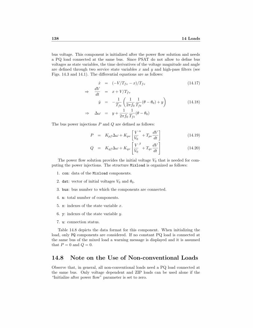
138 14 Loads
bus voltage. This component is initialized after the power flow solution and needsa PQ load connected at the same bus. Since PSAT do not allow to define busvoltages as state variables, the time derivatives of the voltage magnitude and angleare defined through two service state variables x and y and high-pass filters (seeFigs. 14.3 and 14.1). The differential equations are as follows:
x = (−V/Tfv − x)/Tfv (14.17)
⇒ dV
dt= x+ V/Tfv
y = − 1
Tft
(1
2πf0
1
Tft(θ − θ0) + y
)(14.18)
⇒ ∆ω = y +1
2πf0
1
Tft(θ − θ0)
The bus power injections P and Q are defined as follows:
P = Kpf∆ω +Kpv
[V
V0
α
+ TpvdV
dt
](14.19)
Q = Kqf∆ω +Kqv
[V
V0
β
+ TqvdV
dt
](14.20)
The power flow solution provides the initial voltage V0 that is needed for com-puting the power injections. The structure Mixload is organized as follows:
1. con: data of the Mixload components.
2. dat: vector of initial voltages V0 and θ0.
3. bus: bus number to which the components are connected.
4. n: total number of components.
5. x: indexes of the state variable x.
6. y: indexes of the state variable y.
7. u: connection status.
Table 14.8 depicts the data format for this component. When initializing theload, only PQ components are considered. If no constant PQ load is connected atthe same bus of the mixed load a warning message is displayed and it is assumedthat P = 0 and Q = 0.
14.8 Note on the Use of Non-conventional Loads
Observe that, in general, all non-conventional loads need a PQ load connected atthe same bus. Only voltage dependent and ZIP loads can be used alone if the“Initialize after power flow” parameter is set to zero.

14.8 Note on the Use of Non-conventional Loads 139
Table 14.8: Mixed Data Format (Mixload.con)
Column Variable Description Unit1 - Bus number int2 Sn Power rate MVA3 Vn Voltage rate kV4 fn Frequency rate Hz5 Kpv Frequency coefficient for the active power p.u.6 Kpv Percentage of active power %7 α Voltage exponent for the active power -8 Tpv Time constant of dV/dt for the active power s9 Kpv Frequency coefficient for the reactive power p.u.10 Kpv Percentage of reactive power %11 β Voltage exponent for the reactive power -12 Tqv Time constant of dV/dt for the reactive power s13 Tfv Time constant of voltage magnitude filter s14 Tft Time constant of voltage angle filter s15 u Connection status 0, 1
The powers used for initializing non-conventional loads but the exponential re-covery loads are a percentage of the PQ load powers. If the sum of all percentagesis 100%, the PQ load is removed from the data. Observe that PSAT does not checkif the total sum of non-conventional load percentages is greater than 100%. Whenthis happens the resulting PQ load will show negative powers.
Finally, observe that exponential recovery loads are processed last, clearing thePQ load powers. Thus, be aware that when exponential recovery loads and othernon-conventional loads are used together, the actual powers used by exponentialrecovery loads are the powers remaining after the initialization of the other loads(not the initial PQ load powers).
Refer to Section 22.3.8 for details on the usage of non-conventional load withinSimulink models.


Chapter 15
Machines
This chapter describes the synchronous machine and the induction motor models.These components are described by the general equations:
x = f(x, y, u) (15.1)
P = gP (x, y)
Q = gQ(x, y)
where x are the state variables, y the algebraic variables (i.e. V and θ) and u inputvariables.
With regard to the induction motor models, u (i.e. the mechanical torque Tm)is set by the user, and equations (15.1) are included in the power flow analysis.
The synchronous machines are initialized after power flow computations. A PVor a slack generator are required to impose the desired voltage and active power atthe machine bus. Once the power flow solution has been determined, V0, θ0, P0 andQ0 at the generation bus are used for initializing the state and input variables, thelatter being the field voltage vf and the mechanical torque Tm. Thus, the followingsystem is solved:
0 = f(x, y0, u) (15.2)
P0 = gP (x, y0)
Q0 = gQ(x, y0)
At the end of the initialization procedure, the PV and/or slack generators connectedat the generator buses are removed.
Synchronous machines controls such as AVRs or Turbine Governors are notincluded in the machine models. Refer to Chapter 16 for a detailed description ofgenerator control systems.
15.1 Synchronous Machine
The Park-Concordia model is used for synchronous machine equations, whose sche-me is depicted in Fig. 15.1. Various simplification levels are applied, from the
141

142 15 Machines
PSfrag replacements
a
a
a
b
b
b
c
c
c
dq
f
f
δ
ω
Figure 15.1: Synchronous machine scheme.
classical swing equations to an eight order model with field saturation. Fig. 15.2depicts the d and q-axis block diagrams of stator fluxes for the VI order model whileFig. 15.3 illustrates the field saturation characteristic of the synchronous machine.The link between the network phasors and the machine voltage is as follows:
vd = V sin(δ − θ) (15.3)
vq = V cos(δ − θ)
whereas, power injections are expressed in the form:
P = vdid + vqiq (15.4)
Q = vqid − vdiq
The expressions of d and q-axis currents depend on the model, and in general termsare defined as follows:
0 = g1(x, id, id, V, θ) (15.5)
0 = g2(x, id, id, V, θ)
For models III, IV, V.1, V.2 and VI, the field voltage includes a feedback of therotor speed and the active power produced by the machine:
v∗f = vf +Kω(ω − 1) −KP (P (x, V, θ) − P0) (15.6)
whre P0 is the initial electric power generated by the machine. Equation (15.6)implements a simple oscillation stabilizer and is implied where the notation v∗f isused.

PSfrag replacements
+ +
+
++
+
+
+
++
+
+
− −
−
− −
−
−
11
1 1
1−
−ψq
ψd
iq
id
e′q
e′d
e′′q
e′′d
vf
(xd − x′d) − γd (x′d − x′′d) + γd x′′d − xl
(xq − x′q) − γq (x′q − x′′q ) + γq x′′q − xl
d-axis
q-axis
TAA TAA
T ′d0 T ′
d0
sT ′d0 sT ′′
d0
sT ′q0 sT ′′
q0
Figure 15.2: d and q-axis block diagrams of the stator fluxes for the most detailedsynchronous machine model. Coefficients γd and γq are defined as follows:
γd =T ′′
d0
T ′d0
x′′dx′d
(xd − x′d)
γq =T ′′
q0
T ′q0
x′′qx′q
(xq − x′q)
143

PSfrag replacements
Air gap line
1.2
1.0
0.8
ia1
ib1
ia1.2 ib1.2
e′q
xadif
Figure 15.3: Field saturation characteristic of synchronous machines. Saturationfactors are defined as follows:
S(1.0) = 1 − ia1
ib1
S(1.2) = 1 − ia1.2
ib1.2
Note: the saturation curve is linear for e′q < 0.8, whereas it is approximated bymeans of a quadratic interpolation for e′q ≥ 0.8. S(1.0) < S(1.2) should hold toensure the right convexity of the saturation curve. Observe that if the saturationfactors S(1.0) and/or S(1.2) are given, the d-axis additional leakage time constantis assumed TAA = 0.
144

15.1 Synchronous Machine 145
Table 15.1 depicts the complete synchronous machine data format. CoefficientsγP and γQ are used in case of multiple generators connected to the same bus. Inthis case the amount of active and reactive power that each machine has to provideshould be specified. The sum of these coefficients for the machines connected to thesame bus has to be one. PSAT does not check the consistency of these coefficients.By default, γP and γQ are set to 1. If the d-axis additional leakage time constantTAA is omitted, it is assumed TAA = 0. Table 15.2 depicts a quick reference cardfor the usage of time constants and reactances within synchronous machine models.When a time constant or a reactance is not used, it can be zero. PSAT checkstime constants and reactances when initializing machine state variables; if neededtime constants and/or reactances are negative or zero, PSAT will automatically setdefault values and display warning messages.
The synchronous machine is defined in the Syn structure, with the followingfields:
1. con: Synchronous machine data.
2. n: total number of synchronous machines.
3. bus: numbers of buses to which synchronous machines are connected.
4. Pg, Qg: active and reactive powers of the machines.
5. J11, J12, J21, J22: Jacobians of algebraic equations.
6. Gp, Gq: Jacobians of differential equations with respect to V and θ.
7. delta: rotor angle δ indexes.
8. omega: rotor speed ω indexes.
9. e1q: q-axis transient voltage e′q indexes.
10. e1d: d-axis transient voltage e′d indexes.
11. e2q: q-axis subtransient voltage e′′q indexes.
12. e2d: d-axis subtransient voltage e′′d indexes.
13. psiq: q-axis flux ψq indexes.
14. psid: d-axis flux ψd indexes.
15. Pg0: inital electric power generated by the machine.
16. pm: mechanical power/torque Tm.
17. vf: field voltage vf .

Table 15.1: Synchronous Machine Data Format (Syn.con)
Column Variable Description Unit Model1 - Bus number int all2 Sn Power rating MVA all3 Vn Voltage rating kV all4 fn Frequency rating Hz all5 - Machine model - all6 xl Leakage reactance p.u. all7 ra Armature resistance p.u. all8 xd d-axis synchronous reactance p.u. III, IV, V.1, V.2, V.3, VI, VIII9 x′d d-axis transient reactance p.u. II, III, IV, V.1, V.2, V.3, VI, VIII10 x′′d d-axis subtransient reactance p.u. V.2, VI, VIII11 T ′
d0 d-axis open circuit transient time constant s III, IV, V.1, V.2, V.3, VI, VIII12 T ′′
d0 d-axis open circuit subtransient time constant s V.2, VI, VIII13 xq q-axis synchronous reactance p.u. III, IV, V.1, V.2, V.3, VI, VIII14 x′q q-axis transient reactance p.u. IV, V.1, VI, VIII15 x′′q q-axis subtransient reactance p.u. V.2, VI, VIII16 T ′
q0 q-axis open circuit transient time constant s IV, V.1, VI, VIII17 T ′′
q0 q-axis open circuit subtransient time constant s V.1, V.2, VI, VIII18 M = 2H Mechanical starting time (2 × inertia constant) kWs/kVA all19 D Damping coefficient − all† 20 Kω Speed feedback gain gain III, IV, V.1, V.2, VI† 21 KP Active power feedback gain gain III, IV, V.1, V.2, VI† 22 γP Active power ratio at node [0,1] all† 23 γQ Reactive power ratio at node [0,1] all† 24 TAA d-axis additional leakage time constant s V.2, VI, VIII† 25 S(1.0) First saturation factor - III, IV, V.1, V.2, VI, VIII† 26 S(1.2) Second saturation factor - III, IV, V.1, V.2, VI, VIII
† optional fields
146

15.1 Synchronous Machine 147
Table 15.2: Reference table for synchronous machine time constants and reactances.
Order T ′d0 T ′
q0 T ′′d0 T ′′
q0 xd x′d x′′d xq x′q x′′qII X
III X X X X
IV X X X X X X
V.1 X X X X X X X
V.2 X X X X X X X X
V.3 X X X X
VI X X X X X X X X X X
VIII X X X X X X X X X X
15.1.1 Order II
This is the classic electro-mechanical model, with constant amplitude e.m.f. e′q. Thestate variables are δ and ω. The effects of the leakage reactance and the armatureresistance can be included. The differential equations are as follows:
δ = Ωb(ω − 1) (15.7)
ω = (Pm − Pe −D(ω − 1))/M
where the electrical power Pe is defined as follows:
Pe = (vq + raiq)iq + (vd + raid)id (15.8)
Finally, the following relationships between voltages and currents hold:
0 = vq + raiq − e′q + (x′d − xl)id (15.9)
0 = vd + raid − (x′d − xl)iq
The q-axis transient voltage e′q is constant and is stored in the field vf of the Syn
structure as if it were a field voltage. Automatic Voltage Regulators should not beconnected to order II synchronous machines.
15.1.2 Order III
In this model all the q-axis electromagnetic circuits are neglected, whereas a lead-lag transfer function is used for the d-axis inductance. The three state variables δ,ω and e′q are described by the following differential equations:
δ = Ωb(ω − 1) (15.10)
ω = (Pm − Pe −D(ω − 1))/M
e′q = (−fs(e′q) − (xd − x′d)id + v∗f )/T ′
d0
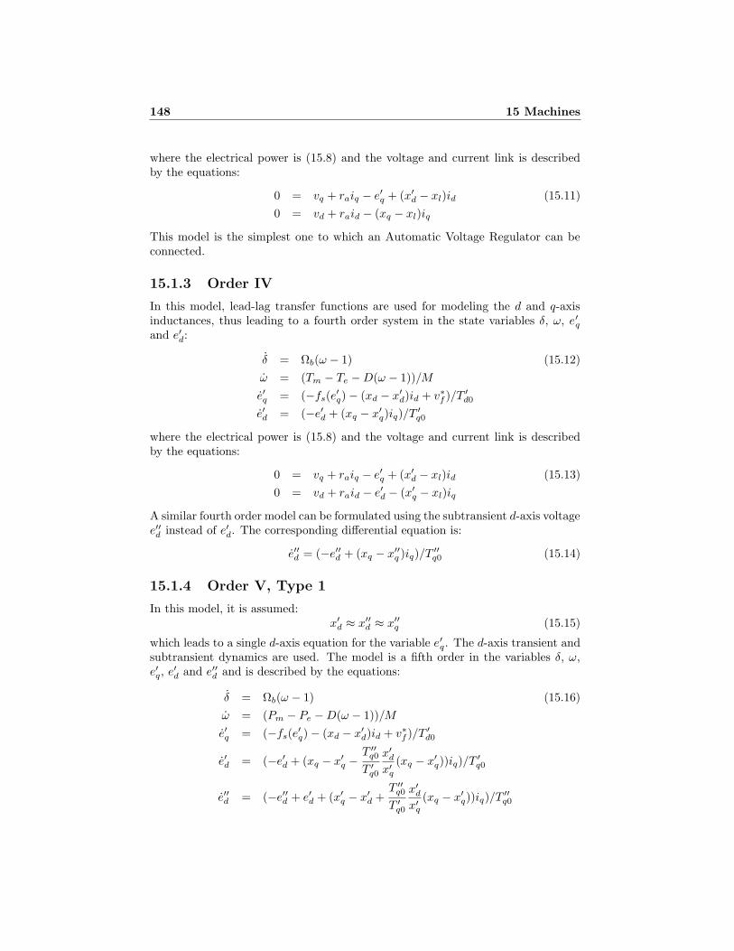
148 15 Machines
where the electrical power is (15.8) and the voltage and current link is describedby the equations:
0 = vq + raiq − e′q + (x′d − xl)id (15.11)
0 = vd + raid − (xq − xl)iq
This model is the simplest one to which an Automatic Voltage Regulator can beconnected.
15.1.3 Order IV
In this model, lead-lag transfer functions are used for modeling the d and q-axisinductances, thus leading to a fourth order system in the state variables δ, ω, e′qand e′d:
δ = Ωb(ω − 1) (15.12)
ω = (Tm − Te −D(ω − 1))/M
e′q = (−fs(e′q) − (xd − x′d)id + v∗f )/T ′
d0
e′d = (−e′d + (xq − x′q)iq)/T′q0
where the electrical power is (15.8) and the voltage and current link is describedby the equations:
0 = vq + raiq − e′q + (x′d − xl)id (15.13)
0 = vd + raid − e′d − (x′q − xl)iq
A similar fourth order model can be formulated using the subtransient d-axis voltagee′′d instead of e′d. The corresponding differential equation is:
e′′d = (−e′′d + (xq − x′′q )iq)/T′′q0 (15.14)
15.1.4 Order V, Type 1
In this model, it is assumed:x′d ≈ x′′d ≈ x′′q (15.15)
which leads to a single d-axis equation for the variable e′q. The d-axis transient andsubtransient dynamics are used. The model is a fifth order in the variables δ, ω,e′q, e
′d and e′′d and is described by the equations:
δ = Ωb(ω − 1) (15.16)
ω = (Pm − Pe −D(ω − 1))/M
e′q = (−fs(e′q) − (xd − x′d)id + v∗f )/T ′
d0
e′d = (−e′d + (xq − x′q −T ′′
q0
T ′q0
x′dx′q
(xq − x′q))iq)/T′q0
e′′d = (−e′′d + e′d + (x′q − x′d +T ′′
q0
T ′q0
x′dx′q
(xq − x′q))iq)/T′′q0
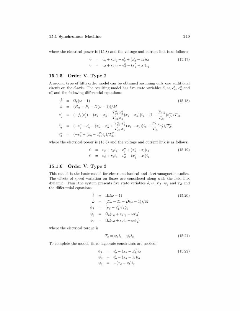
15.1 Synchronous Machine 149
where the electrical power is (15.8) and the voltage and current link is as follows:
0 = vq + raiq − e′q + (x′d − xl)id (15.17)
0 = vd + raid − e′′d − (x′q − xl)iq
15.1.5 Order V, Type 2
A second type of fifth order model can be obtained assuming only one additionalcircuit on the d-axis. The resulting model has five state variables δ, ω, e′q, e
′′q and
e′′d and the following differential equations:
δ = Ωb(ω − 1) (15.18)
ω = (Pm − Pe −D(ω − 1))/M
e′q = (−fs(e′q) − (xd − x′d − T ′′
d0
T ′d0
x′′dx′d
(xd − x′d))id + (1 − TAA
T ′d0
)v∗f )/T ′d0
e′′q = (−e′′q + e′q − (x′d − x′′d +T ′′
d0
T ′d0
x′′dx′d
(xd − x′d))id +TAA
T ′d0
v∗f )/T ′′d0
e′′d = (−e′′d + (xq − x′′q )iq)/T′′q0
where the electrical power is (15.8) and the voltage and current link is as follows:
0 = vq + raiq − e′′q + (x′′d − xl)id (15.19)
0 = vd + raid − e′′d − (x′′q − xl)iq
15.1.6 Order V, Type 3
This model is the basic model for electromechanical and electromagnetic studies.The effects of speed variation on fluxes are considered along with the field fluxdynamic. Thus, the system presents five state variables δ, ω, ψf , ψq and ψd andthe differential equations:
δ = Ωb(ω − 1) (15.20)
ω = (Tm − Te −D(ω − 1))/M
ψf = (vf − e′q)/T′d0
ψq = Ωb(vq + raiq − ωψd)
ψd = Ωb(vd + raid + ωψq)
where the electrical torque is:
Te = ψdiq − ψqid (15.21)
To complete the model, three algebraic constraints are needed:
ψf = e′q − (xd − x′d)id (15.22)
ψd = e′q − (xd − xl)id
ψq = −(xq − xl)iq

150 15 Machines
These equations can be rewritten in order to obtain a differential equation for e′q,thus eliminating from the system the field flux ψf :
e′q =xd − xl
x′d − xl(
1
T ′d0
(vf − e′q) −xd − x′dxd − xl
ψd) (15.23)
The state variables used in PSAT are δ, ω, e′q, ψq and ψd. In order to computecorrect eigenvalues for the small signal stability analysis, this model should be usedin networks where a slack bus is present.
15.1.7 Order VI
The sixth order model is obtained assuming the presence of a field circuit and anadditional circuit along the d-axis and two additional circuits along the q-axis. Thesystem has six state variables (δ, ω, e′q, e
′d, e
′′q and e′′d) and the following equations:
δ = Ωb(ω − 1) (15.24)
ω = (Pm − Pe −D(ω − 1))/M
e′q = (−fs(e′q) − (xd − x′d − T ′′
d0
T ′d0
x′′dx′d
(xd − x′d))id + (1 − TAA
T ′d0
)v∗f )/T ′d0
e′d = (−e′d + (xq − x′q −T ′′
q0
T ′q0
x′′qx′q
(xq − x′q))iq)/T′q0
e′′q = (−e′′q + e′q − (x′d − x′′d +T ′′
d0
T ′d0
x′′dx′d
(xd − x′d))id +TAA
T ′d0
v∗f ))/T ′′d0
e′′d = (−e′′d + e′d + (x′q − x′′q +T ′′
q0
T ′q0
x′′qx′q
(xq − x′q))iq)/T′′q0
where the electrical power is (15.8) and the algebraic constraints are as follows:
0 = vq + raiq − e′′q + (x′′d − xl)id (15.25)
0 = vd + raid − e′′d − (x′′q − xl)iq
This model is basically the same of the VIII order one, but with the assumptionsψd = ψq = 0, ωψd ≈ ψd and ωψq ≈ ψq.
15.1.8 Order VIII
This model is obtained with the same assumption of model VI, but including elec-tromagnetic flux dynamics. The state variables are δ, ω, e′q, e
′d, e
′′q , e′′d , ψd and ψq,

15.2 Induction Motor 151
with the following equations:
δ = Ωb(ω − 1) (15.26)
ω = (Tm − Te −D(ω − 1))/M
e′q = (−fs(e′q) − (xd − x′d − T ′′
d0
T ′d0
x′′dx′d
(xd − x′d))id + (1 − TAA
T ′d0
)vf )/T ′d0
e′d = (−e′d + (xq − x′q −T ′′
q0
T ′q0
x′′qx′q
(xq − x′q))iq)/T′q0
e′′q = (−e′′q + e′q − (x′d − x′′d +T ′′
d0
T ′d0
x′′dx′d
(xd − x′d))id +TAA
T ′d0
vf )/T ′′d0
e′′d = (−e′′d + e′d + (x′q − x′′q +T ′′
q0
T ′q0
x′′qx′q
(xq − x′q))iq)/T′′q0
ψq = Ωb(vq + raiq − ωψd)
ψd = Ωb(vd + raid + ωψq)
where the electrical torque is (15.21). The following algebraic relationship completethe model:
ψd = e′′q − (x′′d − xl)id (15.27)
ψq = −e′′d − (x′′q − xl)iq
In order to compute correct eigenvalues for the small signal stability analysis,this model should be used in networks where a slack bus is present.
15.2 Induction Motor
The models used for the induction motors are defined with an approach similar towhat was described for the synchronous machine. Three models are defined for theinduction motor. These are pure mechanical model, single cage rotor model, anddouble cage rotor model. The expression used for the torque/speed characteristicis a composite load model:
Tm = a+ bω + cω2 (15.28)
and given the relationship between the slip σ and the speed ω in p.u., e.g. σ = 1−ω,the torque/slip characteristic becomes:
Tm = α+ βσ + γσ2 (15.29)
where
α = a+ b+ c
β = −b− 2c
γ = c

152 15 Machines
Table 15.3 depicts the data format of the induction machine. The start-up controlparameter, if enabled, allows fixing σ = 1 for the power flow computation. Aftersolving the power flow, all the start-up parameters are reset to “off”, and theslip is free to vary. This procedure allows computing the start-up transient ofinduction machines. If the start-up is enabled, the initial condition of slips doesnot correspond to a σ = 0. Refer to the following subsections for the detailedmodels of each kind of induction motors. The induction machine is defined in theMot structure, which has the following fields:
1. con: induction motor data.
2. n: total number of induction motors.
3. bus: numbers of buses to which induction motors are connected.
4. dat: induction motor parameters.
5. slip: slip σ indexes.
6. e1r: real part of 1st cage voltage e′r indexes.
7. e1m: imaginary part of 1st cage voltage e′m indexes.
8. e2r: real part of 2st cage voltage e′′r indexes.
9. e2m: imaginary part of 2st cage voltage e′′m indexes.
15.2.1 Order I
The electrical circuit used for the first order induction motor is depicted in Fig. 15.4.Only the mechanical state variable is considered, being the circuit in steady-statecondition. The differential equation is as follows:
σ =1
2Hm
(Tm(σ) − rR1V
2σ
r2R1 + σ2(xS + xR1)2
)(15.30)
whereas the power injections are:
P =rR1V
2σ
r2R1 + σ2(xS + xR1)2(15.31)
Q =V 2
xm+
(xS + xR1)V2σ2
r2R1 + σ2(xS + xR1)2

15.2 Induction Motor 153
Table 15.3: Induction Motor Data Format (Mot.con)
Column Variable Description Unit1 - Bus number int all2 Sn Power rating MVA all3 Vn Voltage rating kV all4 fn Frequency rating Hz all5 - Model order int all6 sup Start-up control boolean all7 rS Stator resistance p.u. III, V8 xS Stator reactance p.u. all9 rR1 1st cage rotor resistance p.u. all10 xR1 1st cage rotor reactance p.u. all11 rR2 2nd cage rotor resistance p.u. V12 xR2 2nd cage rotor reactance p.u. V13 xm Magnetization reactance p.u. all14 Hm Inertia constant kWs/kVA all15 a 1st coeff. of Tm(ω) p.u. all16 b 2nd coeff. of Tm(ω) p.u. all17 c 3rd coeff. of Tm(ω) p.u. all
15.2.2 Order III (single cage)
The simplified electrical circuit used for the single-cage induction motor is depictedin Fig. 15.5. The equations are formulated in terms of the real (r) and imaginary(m) axis, with respect to the network reference angle. In a synchronously rotatingreference frame, the link between the network and the stator machine voltages isas follows:
vr = −V sin θ (15.32)
vm = V cos θ
Using the notation of Fig. 15.5, the power absorptions are:
P = vrir + vmim (15.33)
Q = vmir − vrim
The differential equations in terms of the voltage behind the the stator resistancerS are:
e′r = Ωbσe′m − (e′r + (x0 − x′)im)/T ′
0 (15.34)
e′m = −Ωbσe′r − (e′m − (x0 − x′)ir)/T
′0
whereas the link between voltages, currents and state variables is as follows:
vr − e′r = rSir − x′im (15.35)
vm − e′m = rSim + x′ir
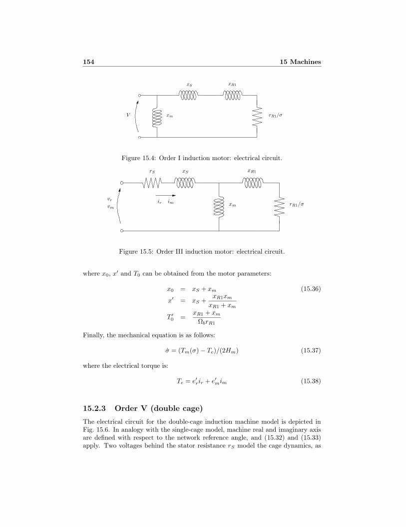
154 15 Machines
PSfrag replacements
V xm
xS xR1
rR1/σ
Figure 15.4: Order I induction motor: electrical circuit.
PSfrag replacements
vr
vm
ir im xm
xSrS xR1
rR1/σ
Figure 15.5: Order III induction motor: electrical circuit.
where x0, x′ and T0 can be obtained from the motor parameters:
x0 = xS + xm (15.36)
x′ = xS +xR1xm
xR1 + xm
T ′0 =
xR1 + xm
ΩbrR1
Finally, the mechanical equation is as follows:
σ = (Tm(σ) − Te)/(2Hm) (15.37)
where the electrical torque is:
Te = e′rir + e′mim (15.38)
15.2.3 Order V (double cage)
The electrical circuit for the double-cage induction machine model is depicted inFig. 15.6. In analogy with the single-cage model, machine real and imaginary axisare defined with respect to the network reference angle, and (15.32) and (15.33)apply. Two voltages behind the stator resistance rS model the cage dynamics, as

15.2 Induction Motor 155
PSfrag replacements
vr
vm
ir im
xm
xSrS
xR1
rR1/σ
xR2
rR2/σ
Figure 15.6: Order V induction motor: electrical circuit.
follows:
e′r = Ωbσe′m − (e′r + (x0 − x′)im)/T ′
0 (15.39)
e′m = −Ωbσe′r − (e′m − (x0 − x′)ir)/T
′0
e′′r = −Ωbσ(e′m − e′′m) + e′r − (e′r − e′′m − (x′ − x′′)im)/T ′′0
e′′m = Ωbσ(e′r − e′′r ) + e′m − (e′m − e′′r + (x′ − x′′)ir)/T′′0
and the links between voltages and currents are:
vr − e′′r = rSir − x′′im (15.40)
vm − e′′m = rSim + x′′ir
where the parameters are determined from the circuit resistances and reactancesand are given by equations (15.36) and:
x′′ = xS +xR1xR2xm
xR1xR2 + xR1xm + xR2xm(15.41)
T ′′0 =
xR2 + xR1xm/(xR1 + xm)
ΩbrR2
The differential equation for the slip is the (15.37), while the electrical torque isdefined as follows:
Te = e′′r ir + e′′mim (15.42)


Chapter 16
Controls
This chapter describes regulators and controllers included in PSAT. These are Tur-bine Governor (TG), Automatic Voltage Regulator (AVR), Power System Stabilizer(PSS), Over Excitation Limiter (OXL), Secondary Voltage Control system whichincludes Central Area Controllers (CACs) and Cluster Controllers (CCs) for coor-dinating AVRs and SVCs, and a Power Oscillation Damper. Control models aredescribed by means of a set of differential equations, as follows:
x = f(x, y, zin) (16.1)
zout = zout(x, y, zin)
where x are the state variable of the component, y the algebraic variables (e.g. busvoltages in case of AVRs), zin are the input variables (e.g. the rotor speed in case ofTGs), and zout are the output variables (e.g. the synchronous machine field voltageand mechanical torque).
16.1 Turbine Governor
Turbine Governors (TGs) define the primary frequency regulation of synchronousmachines. TG data are stored in the structure Tg, as follows:
1. con: Turbine Governor data.
2. n: total number of TGs.
3. syn: generator numbers.
4. dat1: computed parameters for TG type 1.
5. dat2: computed parameters for TG type 2.
6. tg: indexes of state variable tg.
7. tg1: indexes of state variable tg1.
157

158 16 Controls
PSfrag replacements
Governor Servo Reheat
+
+
+
−
ωref
ω
1/R
1
Torder
T ∗in Tin
Tmin
Tmax
Tmech
Tss+ 1
T3s+ 1
Tcs+ 1
T4s+ 1
T5s+ 1
Figure 16.1: Turbine governor type I.
8. tg2: indexes of state variable tg2.
9. tg3: indexes of state variable tg3.
Limits of the mechanical torque are checked at the initialization step. Observethat mechanical torque limits are in p.u. with respect to the machine power rating.If a limit is violated, an error message is displayed and the associated state variablesare not properly initialized.
16.1.1 TG Type I
The TG type I is depicted in Fig. 16.1 and described by the following equations:
T ∗in = Torder +
1
R(ωref − ω) (16.2)
Tin =
T ∗in if Tmin ≤ T ∗
in ≤ Tmax
Tmax if T ∗in > Tmax
Tmin if T ∗in < Tmin
tg1 = (Tin − tg1)/Ts
tg2 = ((1 − T3
Tc)tg1 − tg2)/Tc
tg3 = ((1 − T4
T5)(tg2 +
T3
Tctg1) − tg3)/T5
Tmech = tg3 +T4
T5(tg2 +
T3
Tctg1)
Table 16.1 depicts the data format of the TG type I.
16.1.2 TG Type II
The TG type II is depicted in Fig. 16.2 and described by the following equations:
tg = (1
R(1 − T1
T2)(ωref − ω) − tg)/T2 (16.3)
T ∗mech = tg +
1
R
T1
T2(ωref − ω) + Tmech0

16.2 Automatic Voltage Regulator 159
Table 16.1: Turbine Governor Type I Data Format (Tg.con)
Column Variable Description Unit1 - Generator number int2 1 Turbine governor type int3 ωref Reference speed p.u.4 R Droop p.u./p.u.5 Tmax Maximum turbine output p.u.6 Tmin Minimum turbine output p.u.7 Ts Governor time constant s8 Tc Servo time constant s9 T3 Transient gain time constant s10 T4 Power fraction time constant s11 T5 Reheat time constant sPSfrag replacements
++
+−
ωref
ω
1/R
Tmech0
Tmin
Tmax
TmechT ∗mechT1s+ 1
T2s+ 1
Figure 16.2: Turbine governor type II.
Tmech =
T ∗mech if Tmin ≤ T ∗
mech ≤ Tmax
Tmax if T ∗mech > Tmax
Tmin if T ∗mech < Tmin
Table 16.2 depicts the data format of the TG type II.
16.2 Automatic Voltage Regulator
Automatic Voltage Regulators (AVRs) define the primary voltage regulation ofsynchronous machines. Several AVR models have been proposed and realized inpractice. PSAT allows to define three simple different types of AVRs. AVR TypeI is a standard Italian regulator (ENEL), whereas AVR Type II is the standardIEEE model 1. AVR Type III is the simplest AVR model which can be used forrough stability evaluations. AVRs are stored in the structure Exc, which has thefollowing fields:
1. con: data chart of the Exc components.
2. n: total number of automatic voltage regulators.

160 16 Controls
Table 16.2: Turbine Governor Type II Data Format (Tg.con)
Column Variable Description Unit1 - Generator number int2 2 Turbine governor type int3 ωref Reference speed p.u.4 R Droop p.u./p.u.5 Tmax Maximum turbine output p.u.6 Tmin Minimum turbine output p.u.7 T2 Governor time constant s8 T1 Transient gain time constant s
3. syn: generator numbers.
4. vrif: reference voltage vref.
5. vrif0: reference voltage vref0 (initial value).
6. vr1: indexes of state variable vr1.
7. vr2: indexes of state variable vr2.
8. vr3: indexes of state variable vr3.
9. vm: indexes of state variable vm.
10. vf: indexes of state variable vf .
The reference voltages vref are initialized after the power flow computations.Limits are checked at the initialization step. In case of violation, a warning messageis displayed and AVR state variables are not correctly initialized.
16.2.1 AVR Type I
The AVR Type I is depicted in Fig. 16.3 and described by the following equations:
vm = (V − vm)/Tr (16.4)
vr1 = (µ0(1 − T2
T1)(vref − vm) − vr1)/T1
vr2 = ((1 − T3
T4)(vr1 + µ0
T2
T1(vref − vm)) − vr2)/T4
v∗r = vr2 +T3
T4(vr1 + µ0
T2
T1(vref − vm) + vr1)
vr =
v∗r if vr min ≤ v∗r ≤ vr max,
vr max if v∗r > vr max,
vr min if v∗r < vr min.

16.2 Automatic Voltage Regulator 161
PSfrag replacements
+
+
−
−
vref
V
vm
µ0
vfvrv∗r
vr max
vr min
1
1
Trs+ 1
(T2s+ 1)(T4s+ 1)
(T1s+ 1)(T3s+ 1) Tes+ 1
Se
Figure 16.3: Exciter Type I.
vf = −(vf (1 + Se(vf )) − vr)/Te
where the ceiling function Se is:
Se(vf ) = Ae(eBe|vf | − 1) (16.5)
Table 16.3 depicts the data format of AVR Type I.
16.2.2 AVR Type II
The AVR Type II is depicted in Fig. 16.4 and described by the following equations:
vm = (V − vm)/Tr (16.6)
vr1 = (Ka(vref − vm − vr2 −Kf
Tfvf ) − vr1)/Ta
vr =
vr1 if vr min ≤ vr1 ≤ vr max,
vr max if vr1 > vr max,
vr min if vr1 < vr min.
vr2 = −(Kf
Tfvf + vr2)/Tf
vf = −(vf (1 + Se(vf )) − vr)/Te
where the ceiling function Se is (16.5). The amplifier block is subjected to ananti-windup limit. Table 16.4 depicts the data format of AVR Type II.
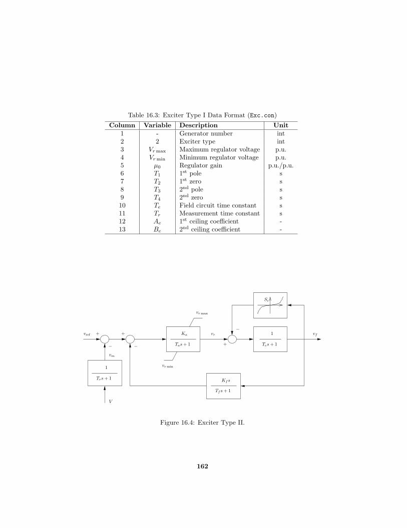
Table 16.3: Exciter Type I Data Format (Exc.con)
Column Variable Description Unit1 - Generator number int2 2 Exciter type int3 Vr max Maximum regulator voltage p.u.4 Vr min Minimum regulator voltage p.u.5 µ0 Regulator gain p.u./p.u.6 T1 1st pole s7 T2 1st zero s8 T3 2nd pole s9 T4 2nd zero s10 Te Field circuit time constant s11 Tr Measurement time constant s12 Ae 1st ceiling coefficient -13 Be 2nd ceiling coefficient -
PSfrag replacements
+ +
+−
−
−
vref
V
vm
Ka
Kfs
vfvr
vr max
vr min1
1
Trs+ 1
Tas+ 1
Tfs+ 1
Tes+ 1
Se
Figure 16.4: Exciter Type II.
162

16.3 Power System Stabilizer 163
Table 16.4: Exciter Type II Data Format (Exc.con)
Column Variable Description Unit1 - Generator number int2 2 Exciter type int3 Vr max Maximum regulator voltage p.u.4 Vr min Minimum regulator voltage p.u.5 Ka Amplifier gain p.u./p.u.6 Ta Amplifier time constant s7 Kf Stabilizer gain p.u./p.u.8 Tf Stabilizer time constant s9 - (not used) -10 Te Field circuit time constant s11 Tr Measurement time constant s12 Ae 1st ceiling coefficient -13 Be 2nd ceiling coefficient -
16.2.3 AVR Type III
The AVR Type III is depicted in Fig. 16.5 and described by the following equations:
vm = (V − vm)/Tr (16.7)
vr = (µ0(1 − T1
T2)(vref − vm) − vr)/T2
vf = ((vr + µ0T1
T2(vref − vm) + vf0)
V
V0− vf )/Tε
The initial field voltage Vf0and bus voltage V0 are set at the initialization step.
The field voltage vf is subjected to an anti-windup limiter and Tε is a fixed smalltime constant (Tε = 0.001 s).1 Table 16.5 depicts the data format of AVR TypeIII.
16.3 Power System Stabilizer
Power System Stabilizers (PSSs) are typically used for damping power system oscil-lations and many different models have been proposed in the literature. In additionto the simple PSS embedded in the synchronous machine equations (models III, IV,V.1, V.2 and VI), five models of PSS are implemented in PSAT.
All models accept as input signals the rotor speed ω, the active power Pg andthe bus voltage magnitude Vg of the generator to which the PSS is connectedthrough the automatic voltage regulator. The PSS output signal is the state variable
1Observe that Tε is not defined by the user. However it can be changed directly in the functionfm exc.m
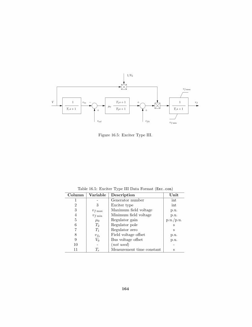
PSfrag replacements
+
+
+
−
vref
V vm
µ0
Kfs
vf
vf0
vr
vf max
vf min
11
Trs+ 1
T1s+ 1
T2s+ 1 Tεs+ 1
1/V0
Figure 16.5: Exciter Type III.
Table 16.5: Exciter Type III Data Format (Exc.con)
Column Variable Description Unit1 - Generator number int2 3 Exciter type int3 vf max Maximum field voltage p.u.4 vf min Minimum field voltage p.u.5 µ0 Regulator gain p.u./p.u.6 T2 Regulator pole s7 T1 Regulator zero s8 vf0
Field voltage offset p.u.9 V0 Bus voltage offset p.u.10 - (not used) -11 Tr Measurement time constant s
164

16.3 Power System Stabilizer 165
vs, which modifies the reference voltage vref of the AVR. the output signal vs
is subjected to an anti-windup limiter and its dynamic is given by a small timeconstant Tε = 0.001 s.2 Note that PSSs cannot be used with order II generators.
PSSs are defined by the structure Pss, as follows:
1. con: PSS data.
2. n: total number of PSSs.
3. bus: bus numbers.
4. syn: synchronous machine numbers.
5. exc: automatic voltage regulator numbers.
6. v1: indexes of the state variable v1.
7. v2: indexes of the state variable v2.
8. v3: indexes of the state variable v3.
9. va: indexes of the state variable va.
10. vss: indexes of the state variable vs.
11. Vs: PSS output signals vs.
12. s1: current status of switches s1.
The complete PSS data format is depicted in Table 16.6.
16.3.1 Type I
PSS Type I is depicted in Fig. 16.6, and is described by the following differentialequation:
v1 = −(Kwω +KpPg +KvVg + v1)/Tw (16.8)
vs = (Kwω +KpPg +KvVg + v1 − vs)/Tε
where ω, Pg and Vg are the rotor speed, the active power and the voltage magnitudeof the generator to which the PSS is connected through the AVR.
2Observe that Tε is not defined by the user. However it can be changed directly in the functionfm pss.m

Table 16.6: Power System Stabilizer Data Format (Pss.con)
Column Variable Description Unit1 - AVR number int all2 - PSS model int all3 - PSS input signal 1 ⇒ ω, 2 ⇒ Pg, 3 ⇒ Vg int II, III, IV, V4 vsmax
Max stabilizer output signal p.u. all5 vsmin
Min stabilizer output signal p.u. all6 Kw Stabilizer gain (used for ω in model I) p.u./p.u. all7 Tw Wash-out time constant s all8 T1 First stabilizer time constant s II, III, IV, V9 T2 Second stabilizer time constant s II, III, IV, V10 T3 Third stabilizer time constant s II, III, IV, V11 T4 Fourth stabilizer time constant s II, III, IV, V12 Ka Gain for additional signal p.u./p.u. IV, V13 Ta Time constant for additional signal s IV, V14 Kp Gain for active power p.u./p.u. I15 Kv Gain for bus voltage magnitude p.u./p.u. I16 vamax
Max additional signal (anti-windup) p.u. IV, V17 v∗amin
Max additional signal (windup) p.u. IV, V18 v∗smax
Max output signal (before adding va) p.u. IV, V19 v∗smin
Min output signal (before adding va) p.u. IV, V20 ethr Field voltage threshold p.u. IV, V21 ωthr Rotor speed threshold p.u. IV, V22 s2 Allow for switch S2 boolean IV, V
166

16.3 Power System Stabilizer 167
PSfrag replacements
++
+
++
vref
vref0Kw
Kp
Kv
ω
Pg
Vg
vs
vs max
vs min
Tws
Tws+ 1
1
Tεs+ 1
Figure 16.6: Power system stabilizer Type I.
PSfrag replacements
Kw
vSI vs
vs max
vs min
Tws
Tws+ 1
T1s+ 1
T2s+ 1
T3s+ 1
T4s+ 1
1
Tεs+ 1
Figure 16.7: Power system stabilizer Type II.
16.3.2 Type II
The PSS Type II is depicted in Fig. 16.7, and is described by the equations:
v1 = −(KwvSI + v1)/Tw (16.9)
v2 = ((1 − T1
T2)(KwvSI + v1) − v2)/T2
v3 = ((1 − T3
T4)(v2 + (
T1
T2(KwvSI + v1))) − v3)/T4
vs = (v3 +T3
T4(v2 +
T1
T2(KwvSI + v1)) − vs)/Tε
16.3.3 Type III
The PSS Type III is depicted in Fig. 16.8, and is described by the equations:
v1 = −(KwvSI + v1)/Tw (16.10)
v2 = a1v3 + a2(KwvSI + v1)
v3 = −v2 + a3v3 + a4(KwvSI + v1)
vs = (v2 +T3
T4(KwvSI + v1) − vs)/Tε

168 16 ControlsPSfrag replacements
Kw
vSI vs
vs max
vs min
Tws
Tws+ 1
T1s2 + T3s+ 1
T2s2 + T4s+ 1
1
Tεs+ 1
Figure 16.8: Power system stabilizer Type III.
where
a1 =1
T4(16.11)
a2 =1
T4(T1 − T2
T3
T4)
a3 = −T2
T4
a4 = 1 − T3
T4− T2
T4(T1 − T2
T3
T4)
16.3.4 Type IV and V
PSS Type IV and V are a slight variation of Type II and III respectively. The blockdiagrams are depicted in Figs. 16.9 and 16.10. The additional signal va is generallydisabled, being the switch S1 open. S1 closes if the machine field voltage is lowerthan a threshold value vf < ethr and remains closed even after vf ≥ ethr. S1 opensif the rotor speed is lower than a threshold value ω < ωthr. It is possible to enablethe action of a second switch S2 after the lag block of the additional signal va. IfS2 is enabled, it stays generally open. S2 closes when the rotor speed deviation∆ω < 0 and remains closed even after ∆ω ≥ 0.
16.4 Over Excitation Limiter
Over excitation limiters (OXLs) provide an additional signal vOXL to the referencevoltage vref0 of automatic voltage regulators (AVRs). It consists in a pure integrator,with anti-windup hard limits, as depicted in Fig. 16.11. This regulator is generallysleeping, i.e. v
OXL= 0, unless the field current is greater than its thermal limit
(if > if lim). The field current is approximated by the following expression:
if =√
(Vg + γq)2 + P 2g + (
xd
xq+ 1)
γq(Vg + γq) + γp√(Vg + γq)2 + P 2
g
(16.12)
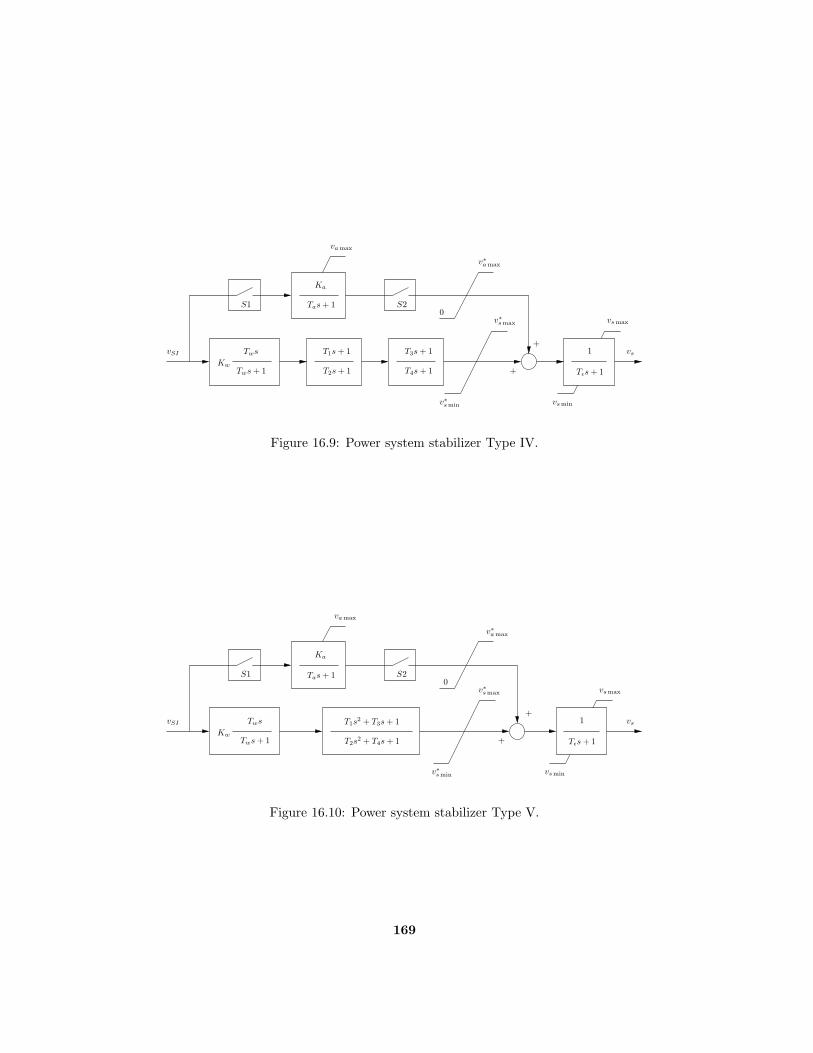
PSfrag replacements
Kw
Ka
vSI
+
+
0S1 S2
vs
vs max
va max
v∗a max
vs min
v∗s max
v∗s min
Tws
Tws+ 1
T1s+ 1
T2s+ 1
T3s+ 1
T4s+ 1
Tas+ 1
1
Tεs+ 1
Figure 16.9: Power system stabilizer Type IV.
PSfrag replacements
Kw
Ka
vSI
+
+
0S1 S2
vs
va max
v∗a max
v∗s max
v∗s min
vs max
vs min
Tws
Tws+ 1
T1s2 + T3s+ 1
T2s2 + T4s+ 1
Tas+ 1
1
Tεs+ 1
Figure 16.10: Power system stabilizer Type V.
169
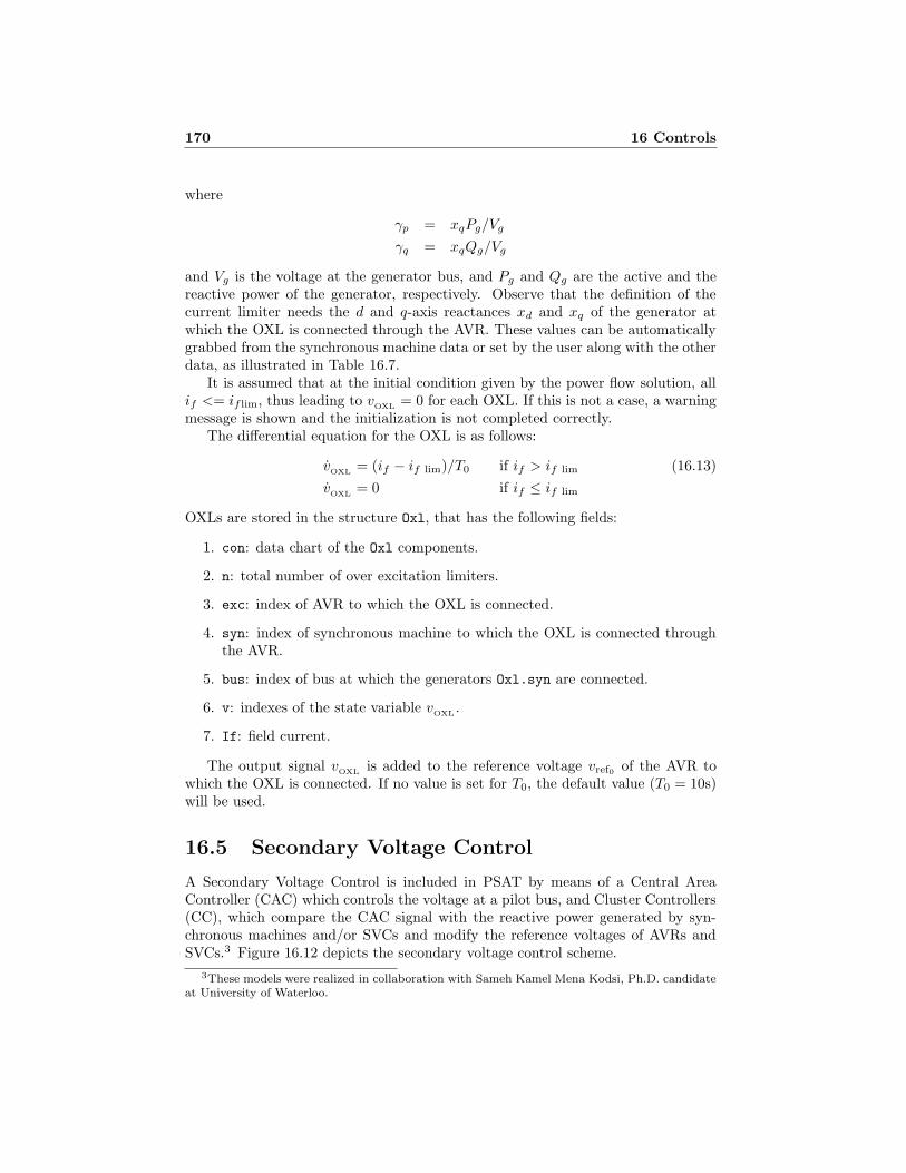
170 16 Controls
where
γp = xqPg/Vg
γq = xqQg/Vg
and Vg is the voltage at the generator bus, and Pg and Qg are the active and thereactive power of the generator, respectively. Observe that the definition of thecurrent limiter needs the d and q-axis reactances xd and xq of the generator atwhich the OXL is connected through the AVR. These values can be automaticallygrabbed from the synchronous machine data or set by the user along with the otherdata, as illustrated in Table 16.7.
It is assumed that at the initial condition given by the power flow solution, allif <= if lim, thus leading to v
OXL= 0 for each OXL. If this is not a case, a warning
message is shown and the initialization is not completed correctly.The differential equation for the OXL is as follows:
vOXL
= (if − if lim)/T0 if if > if lim (16.13)
vOXL
= 0 if if ≤ if lim
OXLs are stored in the structure Oxl, that has the following fields:
1. con: data chart of the Oxl components.
2. n: total number of over excitation limiters.
3. exc: index of AVR to which the OXL is connected.
4. syn: index of synchronous machine to which the OXL is connected throughthe AVR.
5. bus: index of bus at which the generators Oxl.syn are connected.
6. v: indexes of the state variable vOXL
.
7. If: field current.
The output signal vOXL
is added to the reference voltage vref0 of the AVR towhich the OXL is connected. If no value is set for T0, the default value (T0 = 10s)will be used.
16.5 Secondary Voltage Control
A Secondary Voltage Control is included in PSAT by means of a Central AreaController (CAC) which controls the voltage at a pilot bus, and Cluster Controllers(CC), which compare the CAC signal with the reactive power generated by syn-chronous machines and/or SVCs and modify the reference voltages of AVRs andSVCs.3 Figure 16.12 depicts the secondary voltage control scheme.
3These models were realized in collaboration with Sameh Kamel Mena Kodsi, Ph.D. candidateat University of Waterloo.
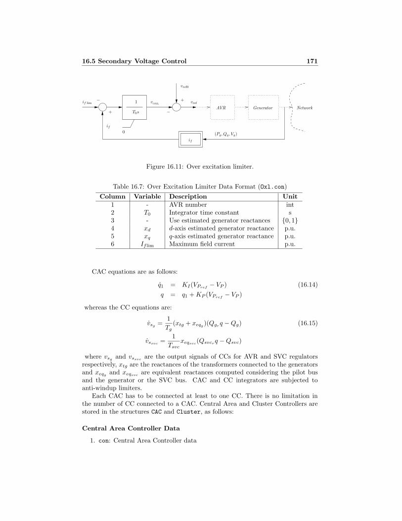
16.5 Secondary Voltage Control 171PSfrag replacements
(Pg, Qg, Vg)
+
+
−
−
0
1
if
if
if lim vOXL
AVR Generator Network
vref0
vref
T0s
Figure 16.11: Over excitation limiter.
Table 16.7: Over Excitation Limiter Data Format (Oxl.con)
Column Variable Description Unit1 - AVR number int2 T0 Integrator time constant s3 - Use estimated generator reactances 0, 14 xd d-axis estimated generator reactance p.u.5 xq q-axis estimated generator reactance p.u.6 If lim Maximum field current p.u.
CAC equations are as follows:
q1 = KI(VPref− VP ) (16.14)
q = q1 +KP (VPref− VP )
whereas the CC equations are:
vsg=
1
Tg(xtg + xeqg
)(Qgrq −Qg) (16.15)
vssvc=
1
Tsvcxeqsvc
(Qsvcrq −Qsvc)
where vsgand vssvc
are the output signals of CCs for AVR and SVC regulatorsrespectively, xtg are the reactances of the transformers connected to the generatorsand xeqg
and xeqsvcare equivalent reactances computed considering the pilot bus
and the generator or the SVC bus. CAC and CC integrators are subjected toanti-windup limiters.
Each CAC has to be connected at least to one CC. There is no limitation inthe number of CC connected to a CAC. Central Area and Cluster Controllers arestored in the structures CAC and Cluster, as follows:
Central Area Controller Data
1. con: Central Area Controller data

_
_
PSfrag replacements
AVR
SVC
Control
NetworkCentral Area Controller
Cluster Controllers
Pilot Bus
+
+ +
+
+ +
+
−
q
q
q
q1max
q1min
KP +KI/s
VP
VPref
KP +KI/s
vsg
vgref
vsg max
vsg min
xtg + xeq
sTg
QgQgr
vssvc
vsvcref
vssvc max
vssvc min
xeq
sTsvc
Qgref
QsvcQsvcr
Qsvcref
Figure 16.12: Secondary voltage control scheme.
172

16.6 Power Oscillation Damper 173
Table 16.8: Central Area Controller Data Format (CAC.con)
Column Variable Description Unit1 - Pilot bus number int2 Sn Power rating MVA3 Vn Voltage rating kV4 - number of connected CC int5 VPref
Reference pilot bus voltage p.u.6 KI Integral control gain p.u.7 KP Proportional control gain p.u.8 q1max
Maximum output signal p.u.9 q1min
Minimum output signal p.u.
2. n: total number of CAC
3. bus: indexes of pilot buses
4. q1: indexes of the state variable q1
Cluster Controller Data
1. con: Cluster Controller data
2. n: total number of CC
3. bus: indexes of generator or SVC buses
4. syn: indexes of generators
5. avr: indexes of AVRs
6. svc: indexes of SVCs
7. Vs: indexes of the state variable Vs
Tables 16.8 and 16.9 depicts the data format of Central Area and Cluster Con-trollers.
16.6 Power Oscillation Damper
This section describes a Power Oscillation Damper (POD). This model has beenimplemented by Hugo M. Ayres and Marcelo S. Castro.4. An important contribu-
4Hugo M. Ayres and Marcelo S. Castro are with Faculdade de Engenharia Eletricae de Computacao, UNICAMP, Brasil. E-mail: [email protected] [email protected]

174 16 Controls
Table 16.9: Cluster Controller Data Format (Cluster.con)
Column Variable Description Unit1 - Central Area Controller number int2 - AVR or SVC number int3 - Control type (1) AVR; (2) SVC int4 Tg (Tsvc) Integral time constant s5 xtg
Generator transformer reactance p.u.6 xeqg
(xeqsvc) Equivalent reactance p.u.
7 Qgr(Qsvcr
) Reactive power ratio p.u.8 Vsmax
Maximum output signal p.u.9 Vsmin
Minimum output signal p.u.
tion was given also by Dr. Alberto Alberto Del Rosso.5 The differential equationsas well as the control scheme of the POD are the same as the PSS Type II (see equa-tions (16.9) and Fig. 16.7). The output signal fo the POD can be used with SVC,TCSC, STATCOM, SSSC and UPFC components (see Chapter 18 for details).
The input signal vSI can be as follows:
1. Bus voltage magnitude V .
2. Line active power flow Pij .
3. Line active power flow Pji.
4. Line current flow Iij .
5. Line current flow Iji.
6. Line reactive power flow Qij .
7. Line reactive power flow Qji.
where i and j indicates “from bus” and “to bus”, respectively. the controlled buscan be any “controllable” bus, i.e. any bus which is not controlled by other controlloops such as LTC transformers. The controlled line can be any transmission lineand any not regulated transformer.
PODs are stored in the structure Pod, that has the following fields:
1. con: data chart of the Pod components.
2. n: total number of PODs.
3. svc: index of SVCs to which the PODs are connected.
5Dr. Alberto Del Rosso is with Mercados Energeticos, Buenos Aires, Madrid, WashingtonD.C. and with National University of Technology, Buenos Aires.E-mail: [email protected]
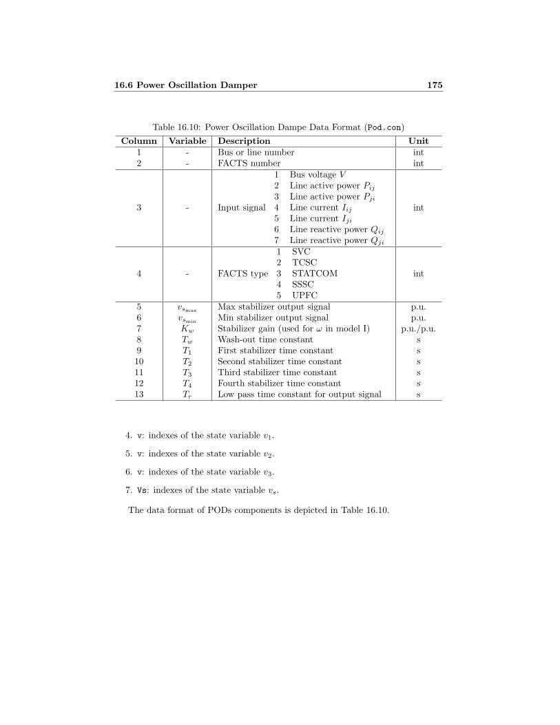
16.6 Power Oscillation Damper 175
Table 16.10: Power Oscillation Dampe Data Format (Pod.con)
Column Variable Description Unit1 - Bus or line number int2 - FACTS number int
3 - Input signal
1 Bus voltage V2 Line active power Pij
3 Line active power Pji
4 Line current Iij5 Line current Iji
6 Line reactive power Qij
7 Line reactive power Qji
int
4 - FACTS type
1 SVC2 TCSC3 STATCOM4 SSSC5 UPFC
int
5 vsmaxMax stabilizer output signal p.u.
6 vsminMin stabilizer output signal p.u.
7 Kw Stabilizer gain (used for ω in model I) p.u./p.u.8 Tw Wash-out time constant s9 T1 First stabilizer time constant s10 T2 Second stabilizer time constant s11 T3 Third stabilizer time constant s12 T4 Fourth stabilizer time constant s13 Tr Low pass time constant for output signal s
4. v: indexes of the state variable v1.
5. v: indexes of the state variable v2.
6. v: indexes of the state variable v3.
7. Vs: indexes of the state variable vs.
The data format of PODs components is depicted in Table 16.10.

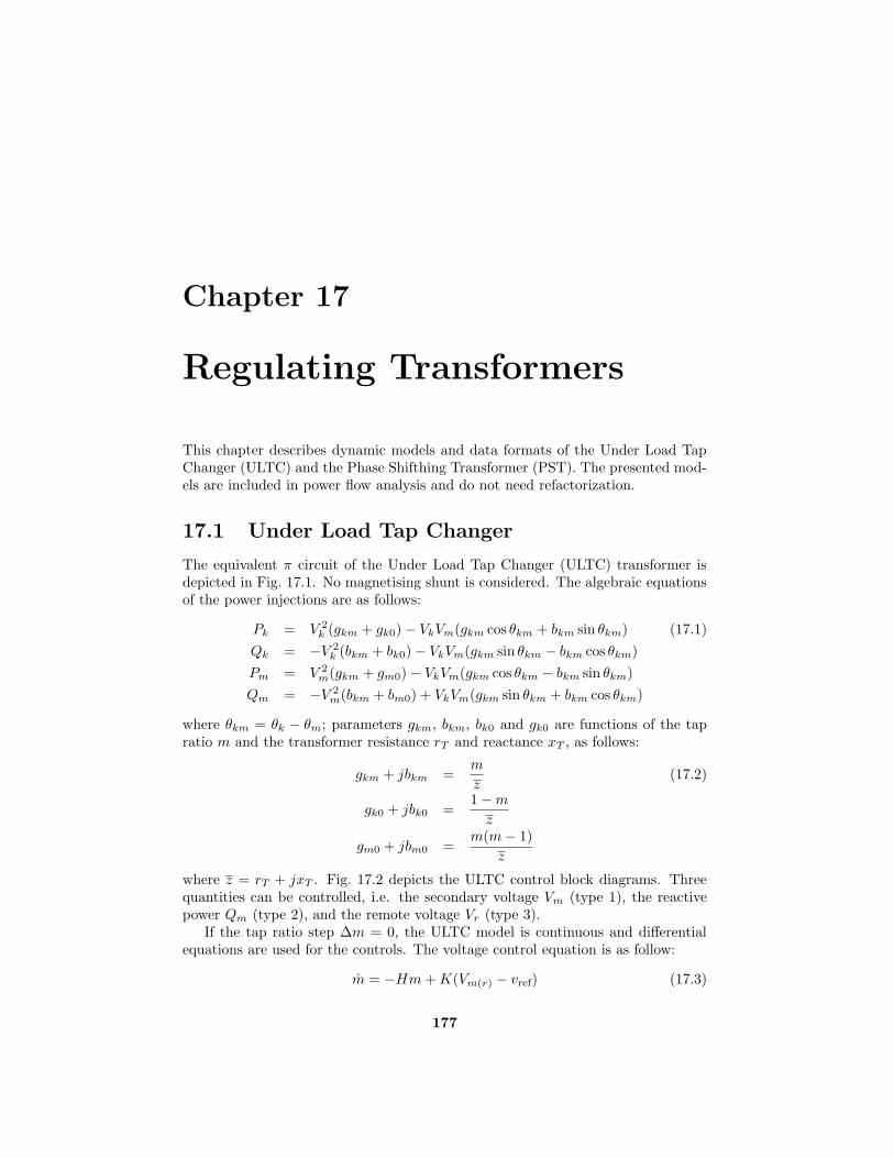
Chapter 17
Regulating Transformers
This chapter describes dynamic models and data formats of the Under Load TapChanger (ULTC) and the Phase Shifthing Transformer (PST). The presented mod-els are included in power flow analysis and do not need refactorization.
17.1 Under Load Tap Changer
The equivalent π circuit of the Under Load Tap Changer (ULTC) transformer isdepicted in Fig. 17.1. No magnetising shunt is considered. The algebraic equationsof the power injections are as follows:
Pk = V 2k (gkm + gk0) − VkVm(gkm cos θkm + bkm sin θkm) (17.1)
Qk = −V 2k (bkm + bk0) − VkVm(gkm sin θkm − bkm cos θkm)
Pm = V 2m(gkm + gm0) − VkVm(gkm cos θkm − bkm sin θkm)
Qm = −V 2m(bkm + bm0) + VkVm(gkm sin θkm + bkm cos θkm)
where θkm = θk − θm; parameters gkm, bkm, bk0 and gk0 are functions of the tapratio m and the transformer resistance rT and reactance xT , as follows:
gkm + jbkm =m
z(17.2)
gk0 + jbk0 =1 −m
z
gm0 + jbm0 =m(m− 1)
z
where z = rT + jxT . Fig. 17.2 depicts the ULTC control block diagrams. Threequantities can be controlled, i.e. the secondary voltage Vm (type 1), the reactivepower Qm (type 2), and the remote voltage Vr (type 3).
If the tap ratio step ∆m = 0, the ULTC model is continuous and differentialequations are used for the controls. The voltage control equation is as follow:
m = −Hm+K(Vm(r) − vref) (17.3)
177
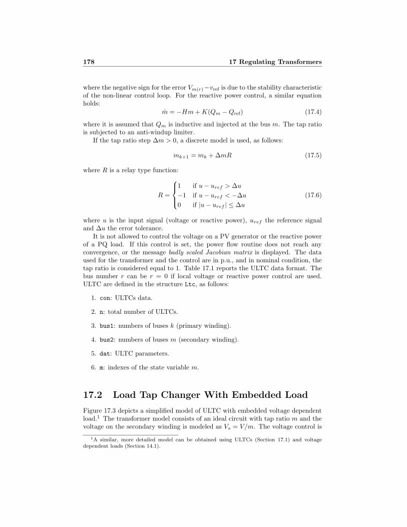
178 17 Regulating Transformers
where the negative sign for the error Vm(r)−vref is due to the stability characteristicof the non-linear control loop. For the reactive power control, a similar equationholds:
m = −Hm+K(Qm −Qref) (17.4)
where it is assumed that Qm is inductive and injected at the bus m. The tap ratiois subjected to an anti-windup limiter.
If the tap ratio step ∆m > 0, a discrete model is used, as follows:
mk+1 = mk + ∆mR (17.5)
where R is a relay type function:
R =
1 if u− uref > ∆u
−1 if u− uref < −∆u
0 if |u− uref | ≤ ∆u
(17.6)
where u is the input signal (voltage or reactive power), uref the reference signaland ∆u the error tolerance.
It is not allowed to control the voltage on a PV generator or the reactive powerof a PQ load. If this control is set, the power flow routine does not reach anyconvergence, or the message badly scaled Jacobian matrix is displayed. The dataused for the transformer and the control are in p.u., and in nominal condition, thetap ratio is considered equal to 1. Table 17.1 reports the ULTC data format. Thebus number r can be r = 0 if local voltage or reactive power control are used.ULTC are defined in the structure Ltc, as follows:
1. con: ULTCs data.
2. n: total number of ULTCs.
3. bus1: numbers of buses k (primary winding).
4. bus2: numbers of buses m (secondary winding).
5. dat: ULTC parameters.
6. m: indexes of the state variable m.
17.2 Load Tap Changer With Embedded Load
Figure 17.3 depicts a simplified model of ULTC with embedded voltage dependentload.1 The transformer model consists of an ideal circuit with tap ratio m and thevoltage on the secondary winding is modeled as Vs = V/m. The voltage control is
1A similar, more detailed model can be obtained using ULTCs (Section 17.1) and voltagedependent loads (Section 14.1).

PSfrag replacements
Vk Vm
z/m
(1 −m)/z m(m− 1)/z
Figure 17.1: Under Load Tap Changer: equivalent π circuit.
PSfrag replacements
+
+
−
−
LTC &
LTC &
Network
Network
K
K
H + s
H + s
Vm (Vr)
Qmk
Vref
Qref
mmax
mmax
mmin
mmin
Figure 17.2: Under Load Tap Changer: voltage and reactive power controls.
179

180 17 Regulating Transformers
Table 17.1: Load Tap Changer Data Format (Ltc.con)
Column Variable Description Unit1 k Bus number (from) int2 m Bus number (to) int3 Sn Power rating MVA4 Vn Voltage rating kV5 fn Frequency rating Hz6 kT Nominal tap ratio kV/kV7 H Integral deviation p.u.8 K Inverse time constant 1/s9 mmax Max tap ratio p.u./p.u.10 mmin Min tap ratio p.u./p.u.11 ∆m Tap ratio step p.u./p.u.12 Vref (Qref) Reference voltage (power) p.u.13 xT Transformer reactance p.u.14 rT Transformer resistance p.u.15 r Remote control bus number int
16 - Control1 Secondary voltage Vm
2 Reactive power Qm
3 Remote voltage Vr
int
obtained by means of a quasi-integral anti-windup regulator. The data format isreported in Table 17.2.
The algebraic equations of the component are as follows:
P = Pn
(V
m
)α
(17.7)
Q = Qn
(V
m
)β
and the scalar differential equation is:
m = −hm+ k
(V
m− vref
)(17.8)
ULTCs with embedded voltage dependent load are defined in the structure Tap,as follows:
1. con: ULTC with embedded load data.
2. bus: number of buses to which the ULTCs are connected.
3. n: total number of ULTCs.
4. m: indexes of the state variable m.

PSfrag replacements
1
P = PnVαs
Q = QnVβs
h+ ks
Vsm : 1V ∠θ
mmax
mmin
Figure 17.3: Load Tap Changer with embedded load.
Table 17.2: Tap Changer with Embedded Load Data Format (Tap.con)
Column Variable Description Unit1 - Bus number int2 Sn Power rating MVA3 Vn Voltage rating kV4 h Deviation from integral behaviour p.u.5 k Inverse of time constant 1/s6 mmin Maximum tap ratio p.u./p.u.7 mmax Minimum tap ratio p.u./p.u.8 vref Reference voltage p.u.9 Pn Nominal active power p.u.10 Qn Nominal reactive power p.u.11 α Voltage exponent (active power) p.u.12 β Voltage exponent (reactive power) p.u.
181
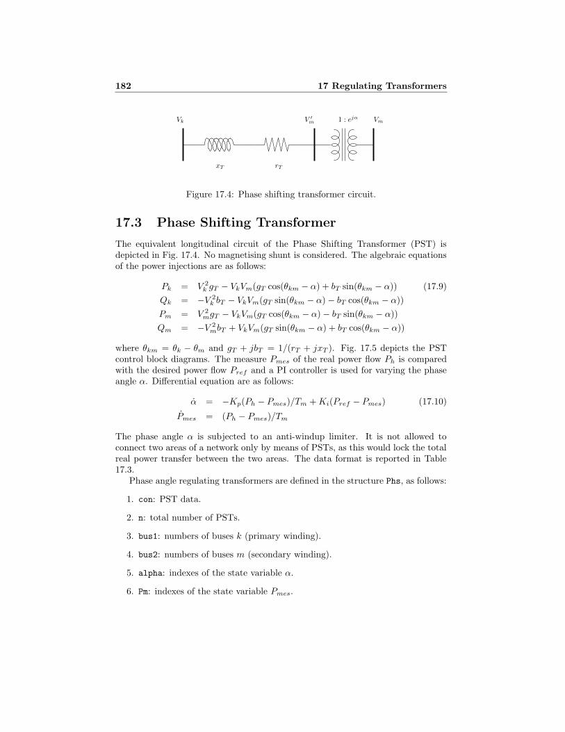
182 17 Regulating Transformers
PSfrag replacements
Vk VmV ′m 1 : ejα
rTxT
Figure 17.4: Phase shifting transformer circuit.
17.3 Phase Shifting Transformer
The equivalent longitudinal circuit of the Phase Shifting Transformer (PST) isdepicted in Fig. 17.4. No magnetising shunt is considered. The algebraic equationsof the power injections are as follows:
Pk = V 2k gT − VkVm(gT cos(θkm − α) + bT sin(θkm − α)) (17.9)
Qk = −V 2k bT − VkVm(gT sin(θkm − α) − bT cos(θkm − α))
Pm = V 2mgT − VkVm(gT cos(θkm − α) − bT sin(θkm − α))
Qm = −V 2mbT + VkVm(gT sin(θkm − α) + bT cos(θkm − α))
where θkm = θk − θm and gT + jbT = 1/(rT + jxT ). Fig. 17.5 depicts the PSTcontrol block diagrams. The measure Pmes of the real power flow Ph is comparedwith the desired power flow Pref and a PI controller is used for varying the phaseangle α. Differential equation are as follows:
α = −Kp(Ph − Pmes)/Tm +Ki(Pref − Pmes) (17.10)
Pmes = (Ph − Pmes)/Tm
The phase angle α is subjected to an anti-windup limiter. It is not allowed toconnect two areas of a network only by means of PSTs, as this would lock the totalreal power transfer between the two areas. The data format is reported in Table17.3.
Phase angle regulating transformers are defined in the structure Phs, as follows:
1. con: PST data.
2. n: total number of PSTs.
3. bus1: numbers of buses k (primary winding).
4. bus2: numbers of buses m (secondary winding).
5. alpha: indexes of the state variable α.
6. Pm: indexes of the state variable Pmes.
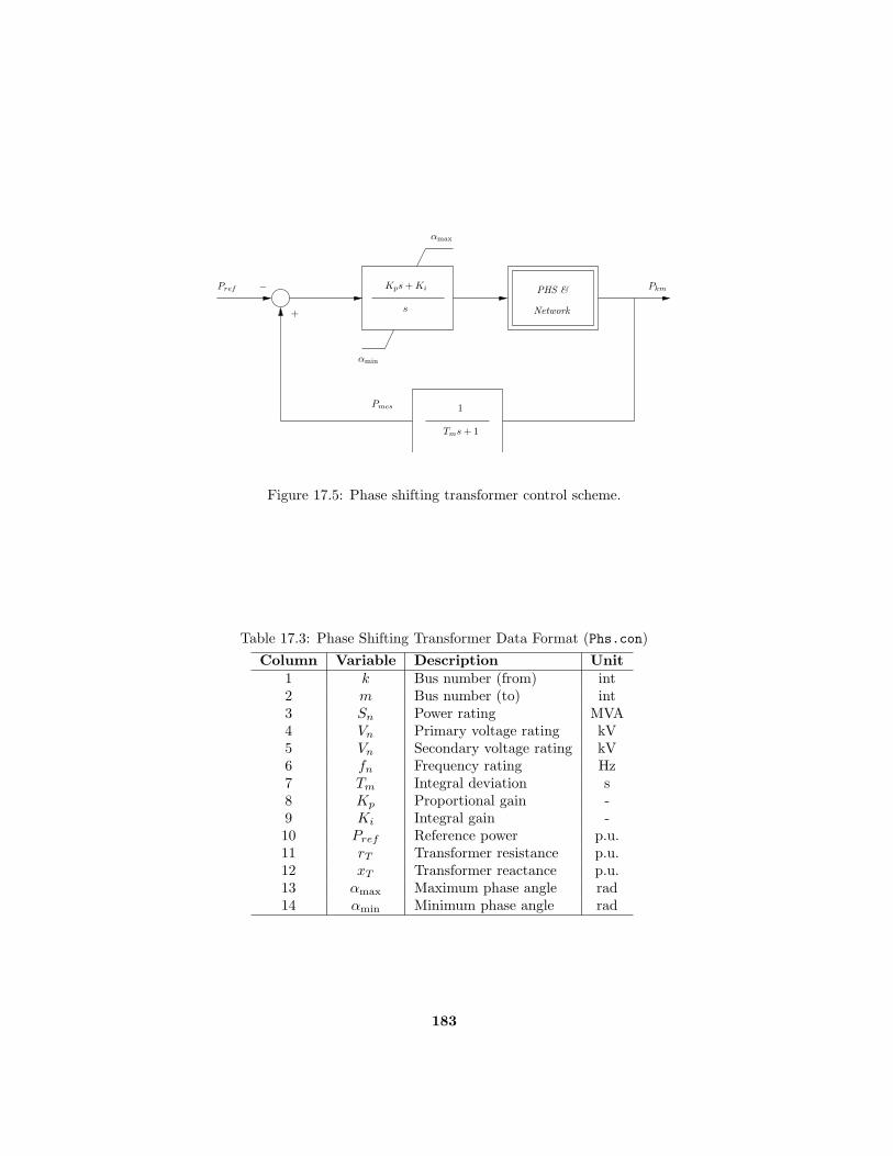
PSfrag replacements
1
s+
− Kps+Ki
Tms+ 1
Vs
m : 1
Pmes
Pref Pkm
αmax
αmin
PHS &
Network
Figure 17.5: Phase shifting transformer control scheme.
Table 17.3: Phase Shifting Transformer Data Format (Phs.con)
Column Variable Description Unit1 k Bus number (from) int2 m Bus number (to) int3 Sn Power rating MVA4 Vn Primary voltage rating kV5 Vn Secondary voltage rating kV6 fn Frequency rating Hz7 Tm Integral deviation s8 Kp Proportional gain -9 Ki Integral gain -10 Pref Reference power p.u.11 rT Transformer resistance p.u.12 xT Transformer reactance p.u.13 αmax Maximum phase angle rad14 αmin Minimum phase angle rad
183

Chapter 18
FACTS
This chapter describes the models of Thyristor Controlled Reactor (TCR) andVoltage Sourced Inverter (VSI) based Flexible ac Transmission System (FACTS)Controllers and High Voltage dc (HVDC) transmission system. In particular, TCRare represented by Static Var Compensator (SVC) and Thyristor Controlled SeriesCompensator (TCSC) , whereas VSI are the Static Var Compensator (STATCOM),the Static Synchronous Source Series Compensator (SSSC) and the Unified PowerFlow Controller (UPFC) . Each model is described by a set of differential algebraicequations:
xc = fc(xc, xs, V, θ, u) (18.1)
xs = fs(xc, xs, V, θ)
P = gp(xc, xs, V, θ)
Q = gp(xc, xs, V, θ)
where xc are the control system variables, xs are the controlled state variables(e.g. firing angles), and the algebraic variables V and θ are the voltage amplitudesand phases at the buses at which the components are connected, they are vectorsin case of series components. Finally, the variables u represent the input controlparameters, such as reference voltages or reference power flows.
Shunt components, i.e. SVCs, STATCOMs and UPFCs, require a PV generatorto be properly initialized. In the case of UPFCs, the PV generator must be placedat the sending end bus.
SVC, TCSC, STATCOM, SSSC and UPFC models have an additional stabilizingsignal vPOD, which is the output of the Power Oscillation Damper described inSection 16.6.
Since version 2, PSAT is provided with new FACTS models, which basically sub-stitute the old ones. These new models have been implemented by Hugo M. Ayresand Marcelo S. Castro.1. An important contribution was given also by Dr. Alberto
1Hugo M. Ayres and Marcelo S. Castro are with Faculdade de Engenharia Eletricae de Computacao, UNICAMP, Brasil. E-mail: [email protected] [email protected]
185

186 18 FACTS
PSfrag replacements
bSVC
bmax
bmin
V
vPOD
+
+
−
Vref
Kr
Trs+ 1
Figure 18.1: SVC Type 1 Regulator.
Alberto Del Rosso.2
18.1 SVC
Two SVC regulators are implemented in the program. The first one assumes a timeconstant regulator, as depicted in Fig. 18.1. In this model, a total reactance bSVC
is assumed and the following differential equation holds:
bSVC = (Kr(Vref + vPOD − V ) − bSVC)/Tr (18.2)
The model is completed by the algebraic equation expressing the reactive powerinjected at the SVC node:
Q = −bSVCV2 (18.3)
The regulator has an anti-windup limiter, thus the reactance bSVC is locked if oneof its limits is reached and the first derivative is set to zero. Table 18.1 reports thedata and control parameter format for the SVC type 1.
The second model takes into account the firing angle α, assuming a balanced,fundamental frequency operation. Thus, the model can be developed with respectto a sinusoidal voltage. The differential and algebraic equations are as follows:
vM = (KMV − vM )/TM (18.4)
α = (−KDα+KT1
T2TM(vM −KMV ) +K(Vref + vPOD − vM ))/T2
Q = −2α− sin 2α− π(2 − xL/xC)
πxLV 2 = −bSVC(α)V 2
The state variable α undergoes an anti-windup limiter.The SVCs state variables are initialized after the power flow solution. To impose
the desired voltages at the compensated buses, a PV generator with zero active
2Dr. Alberto Del Rosso is with Mercados Energeticos, Buenos Aires, Madrid, WashingtonD.C. and with National University of Technology, Buenos Aires.E-mail: [email protected]

18.1 SVC 187PSfrag replacements
α
αmax
αmin
V
vPOD
+
+
−
Vref
vMKM
TMs+ 1
K(T1s+ 1)
T2s+KD
Figure 18.2: SVC Type 2 Regulator.
Table 18.1: SVC Type 1 Data Format (Svc.con)
Column Variable Description Unit1 - Bus number int2 Sn Power rating MVA3 Vn Voltage rating kV4 fn Frequency rating Hz5 1 Model type int6 Tr Regulator time constant s7 Kr Regulator gain p.u./p.u.8 Vref Reference Voltage p.u.9 bmax Maximum susceptance p.u.10 bmin Minimum susceptance p.u.17 u Connection status 0, 1
power should be used. After the power flow solution the PV bus is removed andthe SVC equations are used. During the state variable initialization a check forSVC limits is performed.
Table 18.1 and Fig. 18.2 report the complete data format and the control blockdiagram for the SVC model 2.
Finally, The SVC components are defined in the structure Svc with the followingfields:
1. con: SVC data.
2. n: total number of SVC.
3. bus: SVC bus numbers.
4. bcv: indexes of the state variable bSVC.
5. alpha: indexes of the state variable α.
6. vm: indexes of the state variable vM .

188 18 FACTS
Table 18.2: SVC Type 2 Data Format (Svc.con)
Column Variable Description Unit1 - Bus number int2 Sn Power rating MVA3 Vn Voltage rating kV4 fn Frequency rating Hz5 2 Model type int6 T2 Regulator time constant s7 K Regulator gain p.u./p.u.8 Vref Reference Voltage p.u.9 αf max Maximum firing angle rad10 αf min Minimum firing angle rad11 KD Integral deviation p.u.12 T1 Transient regulator time constant s13 KM Measure gain p.u./p.u.14 TM Measure time delay s15 xL Reactance (inductive) p.u.16 xC Reactance (capacitive) p.u.17 u Connection status 0, 1
7. Be: equivalent admittances bSVC.
8. Vref: voltage references Vref.
9. u: connection status.
18.2 TCSC
TCSC regulator is depicted in Fig. 18.3. The system undergoes the algebraic equa-tions:
Pkm = VkVm(Ykm +B) sin(θk − θm) (18.5)
Pmk = −Pkm
Qkm = V 2k (Ykm +B) − VkVm(Ykm +B) cos(θk − θm)
Qmk = V 2m(Ykm +B) − VkVm(Ykm +B) cos(θk − θm)
where the indexes k and m stand for the sending and recieving bus indices, respec-tively, and Ykm is the admittance of the line at which the TCSC is connected.
The TCSC differential equation are as follows:
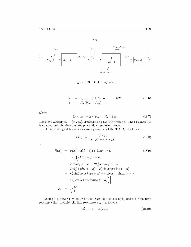
18.2 TCSC 189PSfrag replacements
xc, α B
B(xc, α)
xc max, αmax
xc min, αmin
xc0, α0
vPOD
++
−−
Pref
Pkm Kr
1
Trs+ 1KP +KI/s
Figure 18.3: TCSC Regulator.
x1 = (xc0, α0 +KrvPOD − x1)/Tr (18.6)
x2 = KI(Pkm − Pref)
wherexc0, α0 = KP (Pkm − Pref) + x2 (18.7)
The state variable x1 = xc, α0, depending on the TCSC model. The PI controlleris enabled only for the constant power flow operation mode.
The output signal is the series susceptance B of the TCSC, as follows:
B(xc) = − xc/xkm
xkm(1 − xc/xkm)(18.8)
or
B(α) = π(k4x − 2k2
x + 1) cos kx(π − α)/ (18.9)[xC
(πk4
x cos kx(π − α)
− π cos kx(π − α) − 2k4xα cos kx(π − α)
+ 2αk2x cos kx(π − α) − k4
x sin 2α cos kx(π − α)
+ k2x sin 2α cos kx(π − α) − 4k3
x cos2 α sin kx(π − α)
− 4k2x cosα sinα cos kx(π − α)
)]
kx =
√xC
xL
During the power flow analysis the TCSC is modeled as a constant capacitivereactance that modifies the line reactance xkm, as follows:
x′km = (1 − cp)xkm (18.10)
190 18 FACTS
where cp is the percentage of series compensation. The TCSC state variables areinitaliazed after the power flow analysis as well as the reference power of the PIcontroller Pref. At this step, a check of xc and/or α anti-windup limits is performed.In case of limit violation a warning message is displayed. Table 18.3 reports thedata format of TCSCs components.
The Tcsc class has the following public fields:
1. con: TCSC data.
2. n: total number of TCSCs.
3. line: line number i.
4. bus1: bus numbers k (from).
5. bus2: bus numbers m (to).
6. sscl: indexes of the SSCL connected to the TCSC.
7. x1: indexes of state variables x1.
8. x2: indexes of state variables x2.
9. B: series admittance B.
10. Cp: amount of series compensation cp.
11. x0: initial series reactance x0.
12. Pref: reference power flow Pref.
13. y: line admittance 1/xkm.
14. u: connection status.
The TCSC data format is depicted in Table 18.3.
18.3 STATCOM
The implemented STATCOM model is a current injection model which is basedon [Chun et al. 1998, Rahim et al. 2002, Haque 2004]. The STATCOM current isalways kept in quadrature in relation to the bus voltage so that only reactive poweris exchanged between the ac system and the STATCOM. The dynamic model isshown in Fig. 18.4 where it can be seen that the STATCOM assumes a timeconstant regulator like SVC.
The differential equation and the reactive power injected at the STATCOMnode are given, respectively, by:
iSH = (Kr(Vref + vPOD − V ) − iSH)/Tr (18.11)
Q = −iSHV (18.12)
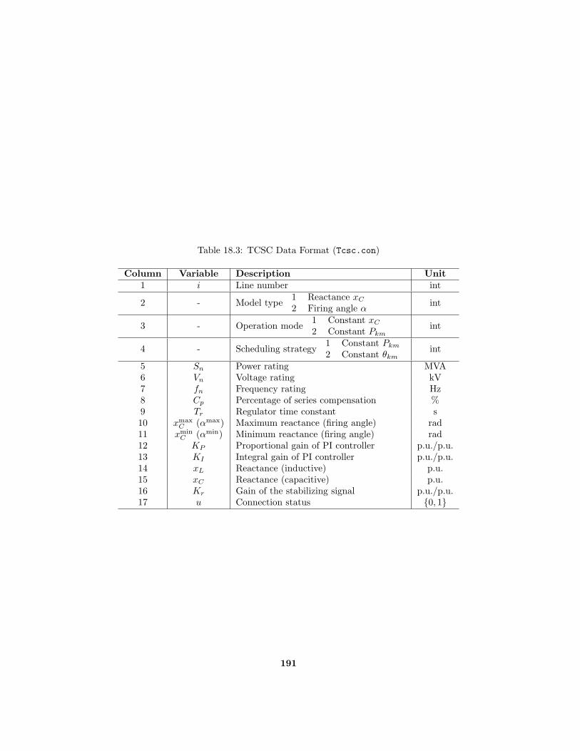
Table 18.3: TCSC Data Format (Tcsc.con)
Column Variable Description Unit1 i Line number int
2 - Model type1 Reactance xC
2 Firing angle αint
3 - Operation mode1 Constant xC
2 Constant Pkmint
4 - Scheduling strategy1 Constant Pkm
2 Constant θkmint
5 Sn Power rating MVA6 Vn Voltage rating kV7 fn Frequency rating Hz8 Cp Percentage of series compensation %9 Tr Regulator time constant s10 xmax
C (αmax) Maximum reactance (firing angle) rad11 xmin
C (αmin) Minimum reactance (firing angle) rad12 KP Proportional gain of PI controller p.u./p.u.13 KI Integral gain of PI controller p.u./p.u.14 xL Reactance (inductive) p.u.15 xC Reactance (capacitive) p.u.16 Kr Gain of the stabilizing signal p.u./p.u.17 u Connection status 0, 1
191

192 18 FACTS
PSfrag replacements
iSH
+−vS
Vk∠θk
iSH
imax
imin
V
vPOD
+
+
−
Vref
Kr
Trs+ 1
Figure 18.4: STATCOM circuit and control block diagram.
Table 18.4: STATCOM Data Format (Statcom.con)
Column Variable Description Unit1 k Bus number int2 Sn Power rating MVA3 Vn Voltage rating kV4 fn Frequency rating Hz5 Tr Regulator time constant s6 Kr Regulator gain p.u./p.u.7 Imax Maximum current p.u.8 Imin Minimum current p.u.9 u Connection status 0, 1
The regulator has an non-windup limiter, thus the current iSH is locked if one ofits limits is reached and the first derivative is set to zero. Table 18.4 reports thedata and control parameters format for the STATCOM block, and its componentsare defined in the structure Statcom with the following fields:
1. con: STATCOM data.
2. n: total number of STATCOM.
3. bus: STATCOM bus numbers.
4. sscl: indexes of the SSCL connected to the STATCOM.
5. ist: indexes of the state variable iSH.
6. Vref: reference voltage of the STATCOM regulator.
7. u: connection status.
The STATCOM data format is depicted in Table 18.4.

18.4 SSSC 193
18.4 SSSC
The implemented SSSC model is based on [Song and Johns 1999, Kumkratug andHaque 2003b, Mihalic and Gabrijel 2004]. The SSSC is represented by a series volt-age source vS , as depicted in Fig. 18.5. The voltage vS is always kept in quadraturewith line current. Thus the only controllable parameter is the magnitude vS . Thetotal active and reactive power flows in a transmission line with a SSSC are asfollows:
Pkm = (1 + ε)VkVm
xkmsin(θk − θm) (18.13)
Pmk = −Pkm
Qkm = (1 + ε)Vk
xkm(Vk − Vm cos(θk − θm)
Qmk = (1 + ε)Vm
xkm(Vm − Vk cos(θk − θm)
whereε =
vS√V 2
k + V 2m − 2Vkvm cos θkm
(18.14)
The SSSC dynamic model is illustrated in Fig. 18.6 and the differential equationthat describes the dynamic behavior of the SSSC is:
vS = (vS0 + vPOD−vS)/Tr (18.15)
The input vS0 determines the SSSC operation mode which in turn determinesthe value of the SSSC voltage vS in steady-state. Three different control modesare implemented for the SSSC: 1) constant voltage, 2) constant reactance, and 3)constant power flow. For each control mode, the input voltage vS0 is given asfollows:
1) Constant voltage: The magnitude of the voltage vS at steady-state is keptconstant independently of the line current, so the input vS0 = const..
2) Constant reactance: The magnitude of the voltage vS varies proportionallyto the line current keeping constant the total impedance (reactance in fact)of the transmission line where the SSSC is installed. In this operation modethe input vS0 is as follows:
vS0 = kxkmIkm (18.16)
where k is the degree of series compensation, Ikm is the magnitude of the linecurrent, and xkm is the reactance of the transmission line.
3) Constant power flow: Constant power control mode: In this mode, the volt-age vS0 is the output of a PI controller used to control the power flow intransmission systems, as shown in Fig. 18.6. Two strategies are implementedfor the constant power flow control mode:
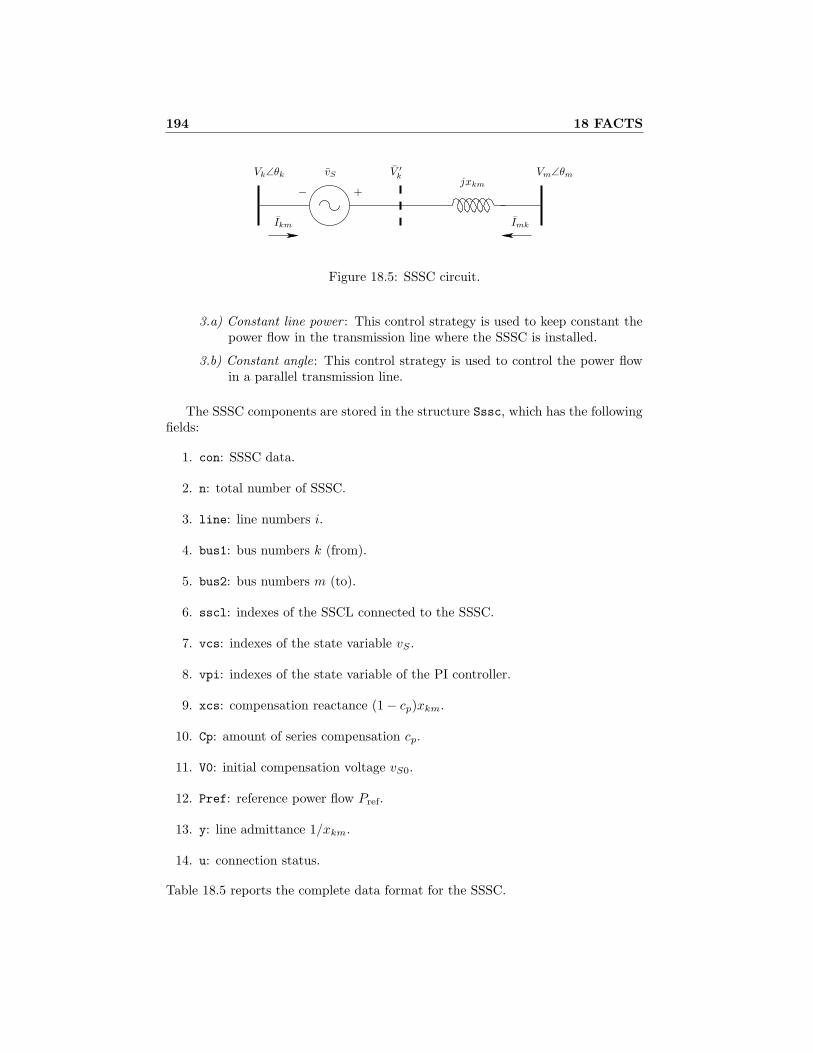
194 18 FACTSPSfrag replacements
Ikm Imk
+−vSVk∠θk V ′
k Vm∠θmjxkm
Figure 18.5: SSSC circuit.
3.a) Constant line power : This control strategy is used to keep constant thepower flow in the transmission line where the SSSC is installed.
3.b) Constant angle: This control strategy is used to control the power flowin a parallel transmission line.
The SSSC components are stored in the structure Sssc, which has the followingfields:
1. con: SSSC data.
2. n: total number of SSSC.
3. line: line numbers i.
4. bus1: bus numbers k (from).
5. bus2: bus numbers m (to).
6. sscl: indexes of the SSCL connected to the SSSC.
7. vcs: indexes of the state variable vS .
8. vpi: indexes of the state variable of the PI controller.
9. xcs: compensation reactance (1 − cp)xkm.
10. Cp: amount of series compensation cp.
11. V0: initial compensation voltage vS0.
12. Pref: reference power flow Pref.
13. y: line admittance 1/xkm.
14. u: connection status.
Table 18.5 reports the complete data format for the SSSC.
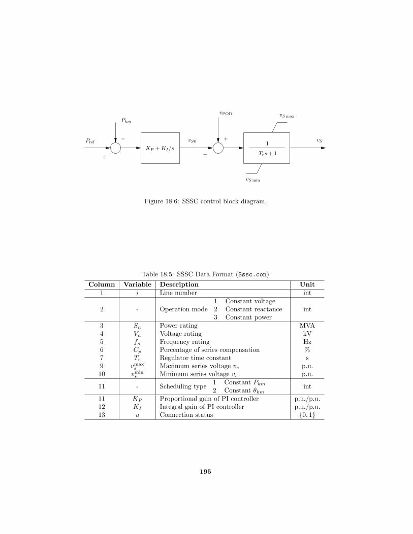
PSfrag replacements
vS
vS max
vS min
vS0
vPOD
+
+
−
−
Pref
Pkm
1
Trs+ 1KP +KI/s
Figure 18.6: SSSC control block diagram.
Table 18.5: SSSC Data Format (Sssc.con)
Column Variable Description Unit1 i Line number int
2 - Operation mode1 Constant voltage2 Constant reactance3 Constant power
int
3 Sn Power rating MVA4 Vn Voltage rating kV5 fn Frequency rating Hz6 Cp Percentage of series compensation %7 Tr Regulator time constant s9 vmax
s Maximum series voltage vs p.u.10 vmin
s Minimum series voltage vs p.u.
11 - Scheduling type1 Constant Pkm
2 Constant θkmint
11 KP Proportional gain of PI controller p.u./p.u.12 KI Integral gain of PI controller p.u./p.u.13 u Connection status 0, 1
195

196 18 FACTS
18.5 UPFC
The implemented UPFC model is based on [Noroozian et al. 1997, Kumkratug andHaque 2003a, Meng and So 2000]. The circuital model of the UPFC is obtainedfrom the STATCOM and SSSC. It is represented by one series voltage source vS
and by one shunt current source iSH, as depicted in Fig. 18.7. The series voltagesource and the shunt current source are defined as follows:
vS = (vp + vq)ejφ = rVke
jγ (18.17)
iSH = (ip + iq)ejθk
The equivalent circuit vector diagram of series voltage source is shown in Fig. 18.8,and the power equations that describe the power injection model of the UPFC are:
Pkm = brVkVm sin(γ + θk − θm) (18.18)
Qkm = brV 2k cos γ − iqVk
Pmk = −brVkVm sin(γ + θk − θm)
Qmk = −brVkVm cos(γ + θk − θm)
The UPFC dynamic model has a 3rd order, as depicted in Fig. 18.9. Observethat the POD controller can be used to modulate whatever of UPFC variables (vp,vq, iq). The set of differential equations are as follows:
vp =1
Tr(vp0 + u1vPOD − vp) (18.19)
vq =1
Tr(vq0 + u2vPOD − vq)
iq =1
Tr[Kr(Vref + u3vPOD − Vk) − iq]
where u1, u2 and u3 are 1 if the correspondent stabilizing POD signal is enabled, 0otherwise.
UPFC State Variables
vp: This variable represents the component of the series voltage vS that is inphase with the line current. In steady-state, the input vp0 is set to zero sothat the exchange of active power between the UPFC and the ac system onlytakes place when this variable is modulated by the POD controller (i.e. duringtransients).
vq: This variable represents the component of series voltage vS that is in quadra-ture with line current. The input vq0 determines the value of the variable vq
in steady-state. Two control modes are implemented for this variable:

18.5 UPFC 197
1. Constant voltage: the magnitude of voltage vq is constant independentlyof the line current;
2. constant reactance: the magnitude of the voltage vq varies proportionallyto the line current keeping constant the total impedance (the resitanceis actually neglected) of the transmission line.
iq: This variable represents the component of shunt current iSH which is inquadrature with the bus voltage Vk. This current keeps the bus voltage arounda specified level through the regulator gain Kr.
The UPFC components are stored in the structure Upfc, which has the followingfields:
1. con: UPFC data.
2. n: total number of UPFC.
3. line: line numbers i.
4. bus1: bus numbers k (from).
5. bus2: bus numbers m (to).
6. sscl: indexes of the SSCL connected to the UPFC.
7. xcs: compensation reactance (1 − cp)xkm.
8. Cp: amount of series compensation cp.
9. vp0: initial compensation voltage vp0.
10. vq0: initial compensation voltage vq0.
11. Vref: reference voltage Vref.
12. y: line admittance 1/xkm.
13. gamma: relative UPFC angle γ.
14. vp: indexes of the state variable vp.
15. vq: indexes of the state variable vq.
16. iq: indexes of the state variable iq.
17. u: connection status.
Table 18.6 illustrates the complete UPFC data format.

PSfrag replacements
Ikm Imk
iSH
+−vSVk∠θk V ′
k Vm∠θmjxkm
Figure 18.7: UPFC circuit.
PSfrag replacements
Ikmref.
vp
vq
vS
Vk γ
θk − φ
Figure 18.8: UPFC phasor diagram.
198
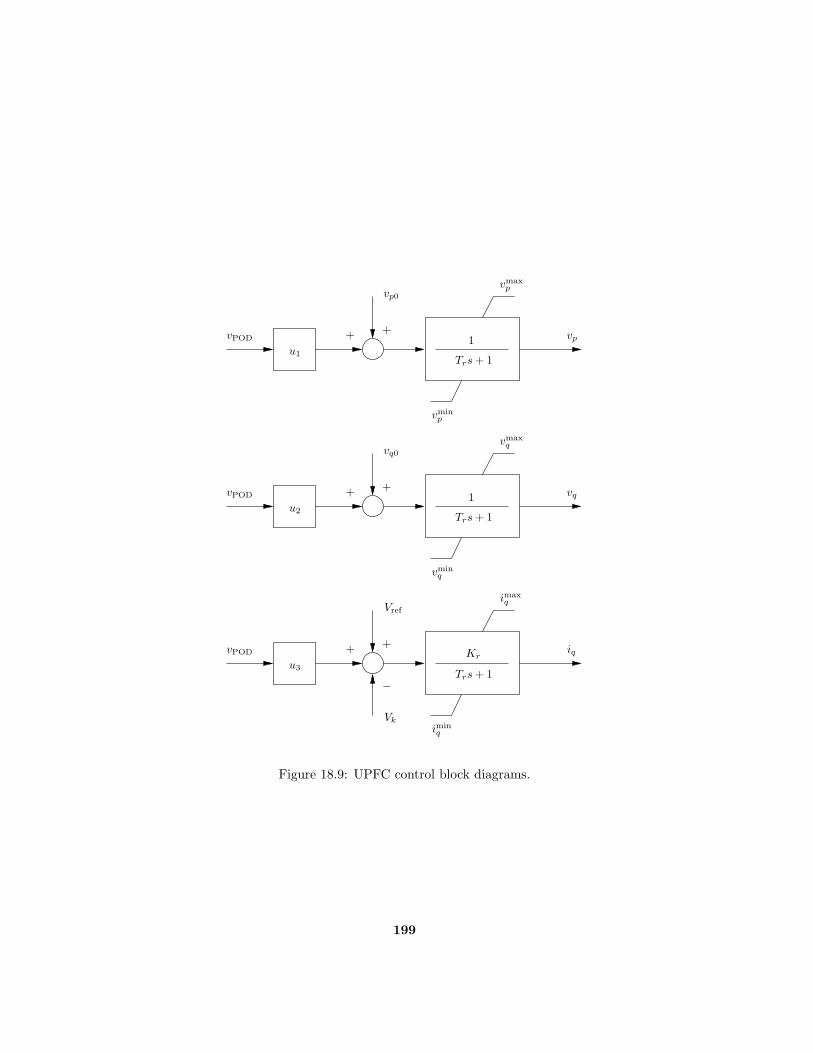
PSfrag replacements
++
++
++
−
1
1
vPOD
vPOD
vPOD
Vk
Vref
u1
u2
u3
vp
vq
vp0
vq0
iq
vmaxp
vminp
vmaxq
vminq
imaxq
iminq
Kr
Trs+ 1
Trs+ 1
Trs+ 1
Figure 18.9: UPFC control block diagrams.
199

Table 18.6: UPFC Data Format (Upfc.con)
Column Variable Description Unit1 i Line number int
2 - Operation mode1 Constant voltage2 Constant reactance
int
3 Sn Power rating MVA4 Vn Voltage rating kV5 fn Frequency rating Hz6 Cp Percentage of series compensation %7 Kr Regulator gain p.u./p.u.8 Tr Regulator time constant s9 vmax
p Maximum vp p.u.10 vmin
p Minimum vp p.u.11 vmax
q Maximum vq p.u.12 vmin
q Minimum vq p.u.13 imax
q Maximum iq p.u.14 imin
q Minimum iq p.u.15 - Stabilizing vp signal 0, 116 - Stabilizing vq signal 0, 117 - Stabilizing iq signal 0, 118 u Connection status 0, 1
200

18.6 HVDC 201
18.6 HVDC
A simple HVDC system is implemented in PSAT, representing two AC/DC con-verters connected by a single DC line. The line is modeled as an RL circuit, whereasthe firing angle α and the extinction angle γ are controlled by PI regulators, as de-picted in Fig. 18.10. The control system regulates the current flow in the DC line.By default the converter connected to the bus k is considered the rectifier, and theother one is the inverter. If the current flow changes direction, the two convertersare switched. The model of the HVDC is as follows:
Idc = (VRdc− VIdc
−RdcIdc)/Ldc (18.20)
xR = KI(IR0 − Idc)
xI = KI(Idc − II0)
Pkm =Vndc
Indc
SnVRdc
Idc
Qkm =
√
S2R −
(Vndc
Indc
SnVRdc
Idc
)2
Pmk =Vndc
Indc
SnVIdc
Idc
Qmk =
√
S2I−
(Vndc
Indc
SnVIdc
Idc
)2
along with the algebraic equations:
cosα = xR +KP (IR0 − Idc) (18.21)
VRdc=
3√
2
πVk cosα− 3
πXtR
Idc
SR =3√
2
π
VndcIndc
SnVkIdc
IR0 =Vk
mR
cos(π − γ) = xI +KP (Idc − II0)
VIdc=
3√
2
πVm cos(π − γ) − 3
πXtI
Idc
SI =3√
2
π
VndcIndc
SnVmIdc
II0 =Vm
mI
The HVDC components are stored in the structure Hvdc, which has the followingfields:
1. con: HVDC data.

202 18 FACTS
Inverter
RectifierPSfrag replacements
+
+
−
−
Idc
Idc
IR0max
IR0min
II0max
II0min
cos(α)
cos(αmax)
cos(αmin)
cos(π − γ)
cos(π − γmax)
cos(π − γmin)
IR0
II0
KP s+KI
KP s+KI
s
s
Figure 18.10: HVDC current control.
2. n: total number of HVDC.
3. bus1: bus numbers k (from).
4. bus2: bus numbers m (to).
5. dat: HVDC parameters.
6. Id: indexes of the state variable Id.
7. Vdc: indexes of the state variable Vdc.
8. xr: indexes of the state variable xr.
9. xi: indexes of the state variable xi.
Table 18.7 reports the complete data format for the HVDC.

Table 18.7: HVDC Data Format (Hvdc.con)
Column Variable Description Unit1 k Bus number (from) int2 m Bus number (to) int3 Sn Power rating MVA4 Vnk
Voltage rating at bus k kV5 Vnm
Voltage rating at bus m kV6 fn Frequency rating Hz7 Vndc
DC voltage rating kV8 Indc
DC current rating kA9 XtR
Transformer reactance (rectifier) p.u.10 XtI
Transformer reactance (inverter) p.u.11 mR Tap ratio (rectifier) p.u.12 mI Tap ratio (inverter) p.u.13 KI Integral gain 1/s14 KP Proportional gain p.u./p.u.15 Rdc Resistance of the DC connection Ω16 Ldc Inductance of the DC connection H17 αR max Maximum firing angle α deg18 αR min Minimum firing angle α deg19 γI max Maximum extinction angle γ deg20 γI min Minimum extinction angle γ deg21 IR0 max Maximum reference current (rectifier) p.u.22 IR0 min Minimum reference current (rectifier) p.u.23 II0 max Maximum reference current (inverter) p.u.24 II0 min Minimum reference current (inverter) p.u.
203


Chapter 19
Wind Turbines
This chapter describes wind turbines and wind speed models. Three models of windturbines are included: constant speed wind turbine with squirrel cage inductiongenerator, variable speed wind turbine with doubly fed (wound rotor) inductiongenerator and variable speed wind turbine with direct drive synchronous generator.Wind speed models are a Weibull distribution and a wind model composed ofaverage speed, ramp, gust and turbulence. Wind speed measurement data can beused as well.
Wind turbines are initialized after power flow computations and a PV generatoris needed to impose the desired voltage and active power at the wind turbine bus.Once the power flow solution has been determined, V0, θ0, P0 and Q0 at the gener-ation bus are used for initializing the state and input variables, the latter being thewind speed vw0, which is used as the average wind speed vwa for the wind speedmodels.
Controls and converter models are included in the wind turbine equations. Windturbine models presented here were mostly based on models discussed in [Slootweg2003].
19.1 Wind Models
Wind speed models included in PSAT are the Weibull distribution and a compositemodel which includes average speed, ramp, gust and turbulence. Real measurementdata can be used as well. Observe that, regardless the wind speed model, the firstvalue of the wind speed sequence will be the initial average speed (vw(t0) = vwa)as computed at the initialization step of the wind turbines (see Section 19.2).
Table 19.1 depicts the data format for wind speed models. Air density ρ at 15Cand standard atmospheric pressure is 1.225 kg/m3, and depends on the altitude (e.g.at 2000 m ρ is 20% lower than at the sea level).
Wind speed time sequences are calculated after solving the power flow andinitializing wind turbine variables. To visualize these sequences, type fm wind(-1)
at the Matlab prompt or use the menu View/Plot wind speeds in the main PSAT
205
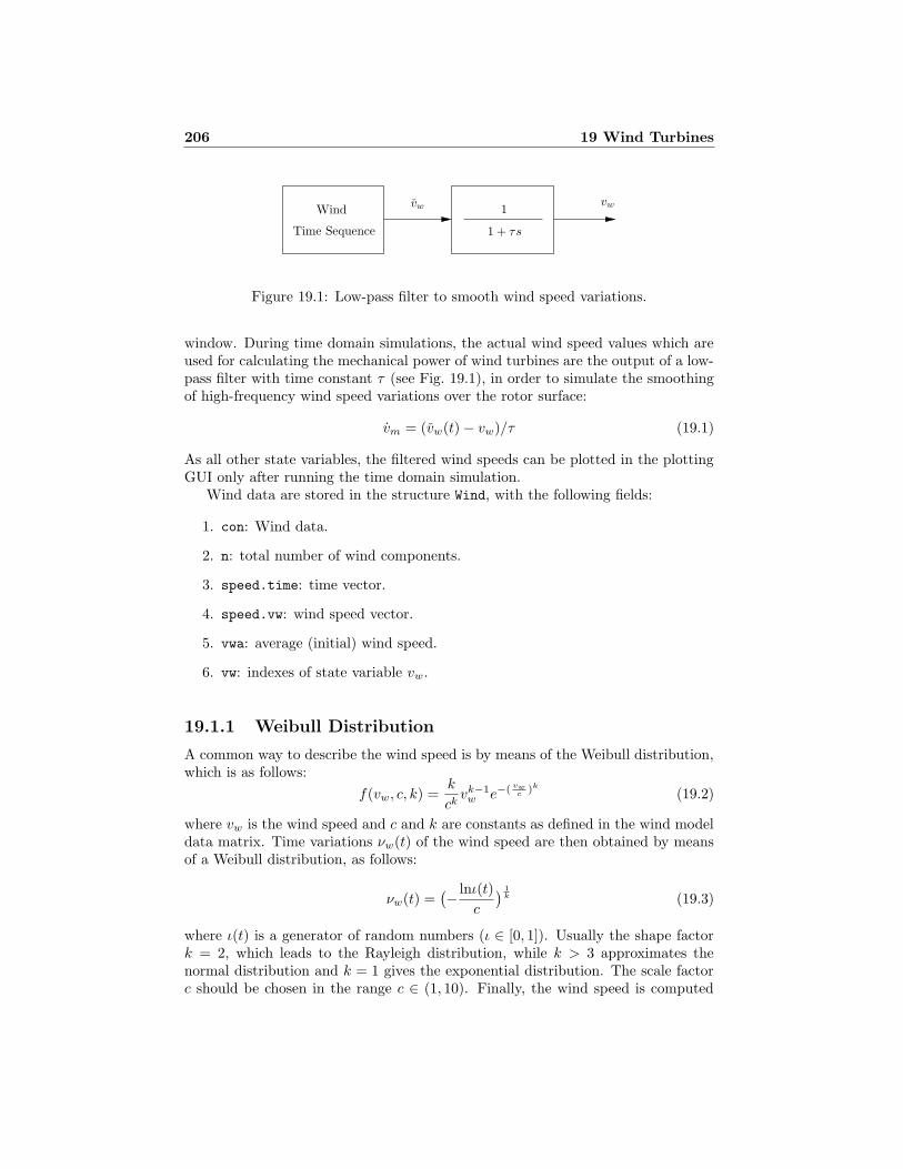
206 19 Wind TurbinesPSfrag replacements
1
1 + τs
vw vwWind
Time Sequence
Figure 19.1: Low-pass filter to smooth wind speed variations.
window. During time domain simulations, the actual wind speed values which areused for calculating the mechanical power of wind turbines are the output of a low-pass filter with time constant τ (see Fig. 19.1), in order to simulate the smoothingof high-frequency wind speed variations over the rotor surface:
vm = (vw(t) − vw)/τ (19.1)
As all other state variables, the filtered wind speeds can be plotted in the plottingGUI only after running the time domain simulation.
Wind data are stored in the structure Wind, with the following fields:
1. con: Wind data.
2. n: total number of wind components.
3. speed.time: time vector.
4. speed.vw: wind speed vector.
5. vwa: average (initial) wind speed.
6. vw: indexes of state variable vw.
19.1.1 Weibull Distribution
A common way to describe the wind speed is by means of the Weibull distribution,which is as follows:
f(vw, c, k) =k
ckvk−1
w e−( vwc
)k
(19.2)
where vw is the wind speed and c and k are constants as defined in the wind modeldata matrix. Time variations νw(t) of the wind speed are then obtained by meansof a Weibull distribution, as follows:
νw(t) =(− lnι(t)
c
) 1
k (19.3)
where ι(t) is a generator of random numbers (ι ∈ [0, 1]). Usually the shape factork = 2, which leads to the Rayleigh distribution, while k > 3 approximates thenormal distribution and k = 1 gives the exponential distribution. The scale factorc should be chosen in the range c ∈ (1, 10). Finally, the wind speed is computed

Table 19.1: Wind Speed Data Format (Wind.con)
Column Variable Description Unit
1 - Wind model1 Measurement data2 Weibull distribution3 Composite model
int
2 vwNNominal wind speed m/s
3 ρ Air density kg/m3
4 τ Filter time constant s5 ∆t Sample time for wind measurements s6 c Scale factor for Weibull distribution -7 k Shape factor for Weibull distribution -8 Tsr Starting ramp time s9 Ter Ending ramp time s10 vwr Ramp speed magnitude m/s11 Tsg Starting gust time s12 Teg Ending gust time s13 vwg Gust speed magnitude m/s14 h Height of the wind speed signal m15 z0 Roughness length m16 ∆f Frequency step Hz17 n Number of harmonics int
207

208 19 Wind Turbines
setting the initial average speed vwa determined at the initialization step as meanspeed:
vw(t) = (1 + νw(t) − νw)vwa (19.4)
where νw is the mean value of νw(t).
19.1.2 Composite Wind Model
A composite wind model is also included in PSAT similar to what proposed in[Wasynczuk et al. 1981, Anderson and Bose 1983]. This model considers the windas composed of four parts, as follows:
1. average and initial wind speed vwa;
2. ramp component of the wind speed vwr;
3. gust component of the wind speed vwg;
4. wind speed turbulence vwt;
thus the resulting wind speed vw is:
vw(t) = vwa + vwr(t) + vwg(t) + vwt(t) (19.5)
where all components are time-dependent except for the initial average speed vwa.
Wind Ramp Component
The wind ramp component is defined by an amplitude Awr and starting and endingtimes, Tsr and Ter respectively:
t < Tsr : vwr(t) = 0 (19.6)
Tsr ≤ t ≤ Ter : vwr(t) = Awr
( t− Tsr
Ter − Tsr
)
t > Ter : vwr(t) = Awr
Wind Gust Component
The wind gust component is defined by an amplitude Awg and starting and endingtimes, Tsg and Teg respectively:
t < Tsg : vwg(t) = 0 (19.7)
Tsg ≤ t ≤ Teg : vwg(t) =Awg
2
(1 − cos
(2π
t− Tsg
Teg − Tsg
))
t > Teg : vwg(t) = Awg
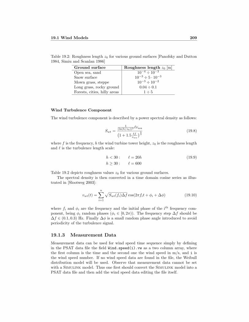
19.1 Wind Models 209
Table 19.2: Roughness length z0 for various ground surfaces [Panofsky and Dutton1984, Simiu and Scanlan 1986]
Ground surface Roughness length z0 [m]Open sea, sand 10−4 ÷ 10−3
Snow surface 10−3 ÷ 5 · 10−3
Mown grass, steppe 10−3 ÷ 10−2
Long grass, rocky ground 0.04 ÷ 0.1Forests, cities, hilly areas 1 ÷ 5
Wind Turbulence Component
The wind turbulence component is described by a power spectral density as follows:
Swt =
1(ln(h/z0))2
`vwa
(1 + 1.5 `f
vwa
) 5
3
(19.8)
where f is the frequency, h the wind turbine tower height, z0 is the roughness lengthand ` is the turbulence length scale:
h < 30 : ` = 20h (19.9)
h ≥ 30 : ` = 600
Table 19.2 depicts roughness values z0 for various ground surfaces.The spectral density is then converted in a time domain cosine series as illus-
trated in [Slootweg 2003]:
vwt(t) =
n∑
i=1
√Swt(fi)∆f cos(2πfit+ φi + ∆φ) (19.10)
where fi and φi are the frequency and the initial phase of the ith frequency com-ponent, being φi random phases (φi ∈ [0, 2π)). The frequency step ∆f should be∆f ∈ (0.1, 0.3) Hz. Finally ∆φ is a small random phase angle introduced to avoidperiodicity of the turbulence signal.
19.1.3 Measurement Data
Measurement data can be used for wind speed time sequence simply by definingin the PSAT data file the field Wind.speed(i).vw as a two column array, wherethe first column is the time and the second one the wind speed in m/s, and i isthe wind speed number. If no wind speed data are found in the file, the Weibulldistribution model will be used. Observe that measurement data cannot be setwith a Simulink model. Thus one first should convert the Simulink model into aPSAT data file and then add the wind speed data editing the file itself.
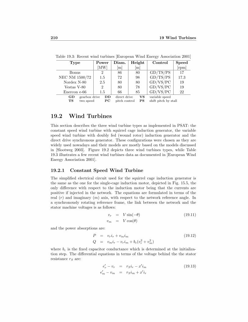
210 19 Wind Turbines
Table 19.3: Recent wind turbines [European Wind Energy Association 2001]
Type Power Diam. Height Control Speed[MW] [m] [m] [rpm]
Bonus 2 86 80 GD/TS/PS 17NEC NM 1500/72 1.5 72 98 GD/TS/PS 17.3
Nordex N-80 2.5 80 80 GD/VS/PC 19Vestas V-80 2 80 78 GD/VS/PC 19Enercon e-66 1.5 66 85 GD/VS/PC 22
GD gearbox drive DD direct drive VS variable speedTS two speed PC pitch control PS shift pitch by stall
19.2 Wind Turbines
This section describes the three wind turbine types as implemented in PSAT: theconstant speed wind turbine with squirrel cage induction generator, the variablespeed wind turbine with doubly fed (wound rotor) induction generator and thedirect drive synchronous generator. These configurations were chosen as they arewidely used nowadays and their models are mostly based on the models discussedin [Slootweg 2003]. Figure 19.2 depicts three wind turbines types, while Table19.3 illustrates a few recent wind turbines data as documented in [European WindEnergy Association 2001].
19.2.1 Constant Speed Wind Turbine
The simplified electrical circuit used for the squirrel cage induction generator isthe same as the one for the single-cage induction motor, depicted in Fig. 15.5, theonly difference with respect to the induction motor being that the currents arepositive if injected in the network. The equations are formulated in terms of thereal (r) and imaginary (m) axis, with respect to the network reference angle. Ina synchronously rotating reference frame, the link between the network and thestator machine voltages is as follows:
vr = V sin(−θ) (19.11)
vm = V cos(θ)
and the power absorptions are:
P = vrir + vmim (19.12)
Q = vmir − vrim + bc(v2r + v2
m)
where bc is the fixed capacitor conductance which is determined at the initializa-tion step. The differential equations in terms of the voltage behind the the statorresistance rS are:
e′r − vr = rSir − x′im (19.13)
e′m − vm = rSim + x′ir

PSfrag replacements
Grid
Grid
Grid
Capacitors
Vs
Vs
Vs
Is
Is
Is
Vr Ir
Vc
Ic
Ic
induction
induction
synchronous
Direct drive
Doubly fed
Squirrel cage
generator
generator
generator
Gear box
Gear box
Rotor
Rotor
Rotor
Converter
Converter
(a)
(b)
(c)
Figure 19.2: Wind turbine types. (a) Constant speed wind turbine with squirrelcage induction generator; (b) Variable speed wind turbine with doubly fed in-duction generator; (c) Variable speed wind turbine with direct drive synchronousgenerator.
211

212 19 Wind Turbines
whereas the link between voltages, currents and state variables is as follows:
e′r = Ωb(1 − ωm)e′m − (e′r − (x0 − x′)im)/T ′0 (19.14)
e′m = −Ωb(1 − ωm)e′r − (e′m + (x0 − x′)ir)/T′0
where x0, x′ and T0 can be obtained from the generator parameters:
x0 = xS + xm (19.15)
x′ = xS +xRxm
xR + xm
T ′0 =
xR + xm
ΩbrR
The mechanical differential equations which take into account the turbine and rotorinertias Hwr and Hm, respectively, and shaft stiffness Ks are as follows:
ωwr = (Twr −Ksγ)/(2Hwr) (19.16)
ωm = (Ksγ − Te)/(2Hm)
γ = Ωb(ωwr − ωm)
where the electrical torque Te is:
Te = e′rir + e′mim (19.17)
The mechanical torque is:
Twr =Pw
ωwr(19.18)
being Pw the mechanical power extracted from the wind. The latter is a functionof both the wind and the rotor speeds and can be approximated as follows:
Pw =ρ
2cp(λ)Arv
3w (19.19)
in which ρ is the air density, cp the performance coefficient or power coefficient, λthe tip speed ratio and Ar the area swept by the rotor. The speed tip ratio λ is theratio between the blade tip speed vt and the wind upstream the rotor vw:
λ =vt
vw= ηGB
2Rωwr
pvw(19.20)
where ηGB is the gear box ratio, p the number of poles of the induction generatorand R the rotor radius. Finally, the the cp(λ) curve is approximated as follows:
cp = 0.44
(125
λi− 6.94
)e− 16.5
λi (19.21)
with
λi =1
1λ + 0.002
(19.22)

19.2 Wind Turbines 213
To simulate the tower shadow effect, a periodic torque pulsation is added to Twr,whose frequency depends on the rotor speed ωwr, the gear box ratio ηGB , and thenumber of blades nb, as follows:
Twr = Twr
(1 + 0.025 sin
(ηGB
Ωbωwr
nbt))
(19.23)
where the torque pulsation amplitude is fixed to 0.025 according to what was pre-sented in [Akhmatov et al. 2000].
The constant speed wind turbine with squirrel cage induction generator is de-fined in the Cswt structure, which has the following fields:
1. con: constant speed wind turbine data.
2. n: total number of constant speed wind turbines.
3. bus: numbers of buses to which wind turbines are connected.
4. wind: numbers of wind speed models to which wind turbines are connected.
5. dat: wind turbines parameters.
6. omega wr: indexes of the state variable ωwr.
7. omega m: indexes of the state variable ωm.
8. gamma: indexes of the state variable γ.
9. e1r: indexes of the state variable e′r.
10. e1m: indexes of the state variable e′m.
Table 19.4 depicts the data format of the constant speed wind turbine with squirrelcage induction generator.
19.2.2 Doubly Fed Induction Generator
Steady-state electrical equations of the doubly fed induction generator are assumed,as the stator and rotor flux dynamics are fast in comparison with grid dynamicsand the converter controls basically decouple the generator from the grid. As aresult of these assumptions, one has:
vds = −rSids + ((xS + xm)iqs + xmiqr) (19.24)
vqs = −rSiqs − ((xS + xm)ids + xmidr)
vdr = −rRidr + (1 − ωm)((xR + xm)iqr + xmiqs)
vqr = −rRiqr − (1 − ωm)((xR + xm)idr + xmids)
where the stator voltages are functions of the grid voltage magnitude and phase:
vds = V sin(−θ) (19.25)
vqs = V cos(θ)
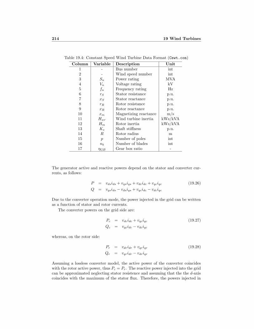
214 19 Wind Turbines
Table 19.4: Constant Speed Wind Turbine Data Format (Cswt.con)
Column Variable Description Unit1 - Bus number int2 - Wind speed number int3 Sn Power rating MVA4 Vn Voltage rating kV5 fn Frequency rating Hz6 rS Stator resistance p.u.7 xS Stator reactance p.u.8 rR Rotor resistance p.u.9 xR Rotor reactance p.u.10 xm Magnetizing reactance m/s11 Hwr Wind turbine inertia kWs/kVA12 Hm Rotor inertia kWs/kVA13 Ks Shaft stiffness p.u.14 R Rotor radius m15 p Number of poles int16 nb Number of blades int17 ηGB Gear box ratio -
The generator active and reactive powers depend on the stator and converter cur-rents, as follows:
P = vdsids + vqsiqs + vdcidc + vqciqc (19.26)
Q = vqsids − vdsiqs + vqcidc − vdciqc
Due to the converter operation mode, the power injected in the grid can be writtenas a function of stator and rotor currents.
The converter powers on the grid side are:
Pc = vdcidc + vqciqc (19.27)
Qc = vqcidc − vdciqc
whereas, on the rotor side:
Pr = vdridr + vqriqr (19.28)
Qr = vqridr − vdriqr
Assuming a lossless converter model, the active power of the converter coincideswith the rotor active power, thus Pc = Pr. The reactive power injected into the gridcan be approximated neglecting stator resistence and assuming that the the d-axiscoincides with the maximum of the stator flux. Therefore, the powers injected in

19.2 Wind Turbines 215
the grid result:
P = vdsids + vqsiqs + vdridr + vqriqr (19.29)
Q = − xmV idr
xS + xm− V 2
xm
The generator motion equation is modeled as a single shaft, as it is assumedthat the converter controls are able to filter shaft dynamics. For the same reason,no tower shadow effect is considered in this model. Thus one has:
ωm = (Tm − Te)/2Hm (19.30)
Te = ψdsiqs − ψqsids
where the link between stator fluxes and generator currents is as follows:
ψds = −((xS + xm)ids + xmidr) (19.31)
ψqs = −((xS + xm)iqs + xmiqr)
Thus the electrical torque Te results:
Te = xm(iqrids − idriqs) (19.32)
To simplify computations, the electrical torque Te is approximated as follows:
Te ≈ − xmV iqr
ωb(xS + xm)(19.33)
where ωb is the system frequency rate in rad/s. The mechanical torque is:
Tm =Pw
ωm(19.34)
being Pw the mechanical power extracted from the wind. The latter is a functionof the wind speed vw, the rotor speed ωm and the pitch angle θp. Pw can beapproximated as follows:
Pw =ρ
2cp(λ, θp)Arv
3w (19.35)
in which parameters and variables are the same as in (19.19) and the speed tipratio λ is defined as in (19.20). The cp(λ, θp) curve is approximated as follows:
cp = 0.22
(116
λi− 0.4θp − 5
)e− 12.5
λi (19.36)
with1
λi=
1
λ+ 0.08θp− 0.035
θ3p + 1(19.37)
Converter dynamics are highly simplified, as they are fast with respect to theelectromechanical transients. Thus, the converter is modeled as an ideal current

216 19 Wind Turbines
source, where iqr and idr are state variables and are used for the rotor speed controland the voltage control respectively, which are depicted in Figures 19.3 and 19.4.Differential equations for the converter currents are as follows:
iqr =(−xs + xm
xmVP ∗
w(ωm)/ωm − iqr
) 1
Tε(19.38)
idr = KV (V − Vref) − V/xm − idr
where P ∗w(ωm) is the power-speed characteristic which roughly optimizes the wind
energy capture and is calculated using the current rotor speed value (see Fig. 19.5).It is assumed that P ∗
w = 0 if ωm < 0.5 p.u. and that P ∗w = 1 p.u. if ωm > 1
p.u. Thus, the rotor speed control only has effect for sub-synchronous speeds.Both the speed and voltage controls undergo anti-windup limiters in order to avoidconverter over-currents. Rotor current limits are computed based on active andreactive limits, and assuming bus voltage V ≈ 1 as follows:
iqrmax≈ −xS + xm
xmPmin (19.39)
iqrmin≈ −xS + xm
xmPmax
idrmax≈ −xS + xm
xmQmin − 1
xm
idrmin≈ −xS + xm
xmQmax − 1
xm
Finally the pitch angle control is illustrated in Fig. 19.6 and described by thedifferential equation:
θp = (Kpφ(ωm − ωref) − θp)/Tp (19.40)
where φ is a function which allows varying the pitch angle set point only when thedifference (ωm − ωref) exceeds a predefined value ±∆ω. The pitch control worksonly for super-synchronous speeds. An anti-windup limiter locks the pitch angle toθp = 0 for sub-synchronous speeds.
The wind turbine with doubly fed induction generator is defined in the Dfig
structure, which has the following fields:
1. con: doubly fed induction generator data.
2. n: total number of doubly fed induction generators.
3. bus: numbers of buses to which generators are connected.
4. wind: numbers of wind speed models to which generators are connected.
5. dat: generator parameters.

PSfrag replacements
iqr
iqrmax
iqrmin
ωm
ωm
T ∗mP ∗
w
P ∗w −(xS + xm)
xmV (1 + sTε)
Figure 19.3: Rotor speed control scheme.
PSfrag replacements
idr
idrmax
idrmin
V
Vref
KV
1
1 + s
−1
xm
++
+−
Figure 19.4: Voltage control scheme.
0.4 0.5 0.6 0.7 0.8 0.9 1 1.10
0.2
0.4
0.6
0.8
1
PSfrag replacements
ωm [p.u.]
P∗ w
[p.u
.]
Figure 19.5: Power-speed characteristic.
217

218 19 Wind Turbines
PSfrag replacements
θpωm
0
ωref
Kp
1 + Tps
+
−
Figure 19.6: Pitch angle control scheme.
6. omega m: indexes of the state variable ωm.
7. theta p: indexes of the state variable θp.
8. idr: indexes of the state variable idr.
9. iqr: indexes of the state variable iqr.
Table 19.5 depicts the data format of the wind turbine with doubly fed inductiongenerator.
19.2.3 Direct Drive Synchronous Generator
Steady-state electrical equations of the direct drive synchronous generator are as-sumed, as the stator and rotor flux dynamics are fast in comparison with grid dy-namics and the converter controls basically decouple the generator from the grid.As a result of these assumptions, one has:
vds = −rsids + ωmxqiqs (19.41)
vqs = −rsiqs − ωm(xdids − ψp)
where a permanent field flux ψp is used here to represent the rotor circuit. Theactive and reactive power of the generator are as follows:
Ps = vdsids + vqsiqs (19.42)
Qs = vqsids − vdsiqs
while the active and reactive powers injected into the grid depend only on the gridside currents of the converter:
Pc = vdcidc + vqciqc (19.43)
Qc = vqcidc − vdciqc
where the converter voltages are functions of the grid voltage magnitude and phase,as follows:
vdc = V sin(−θ) (19.44)
vqc = V cos(θ)
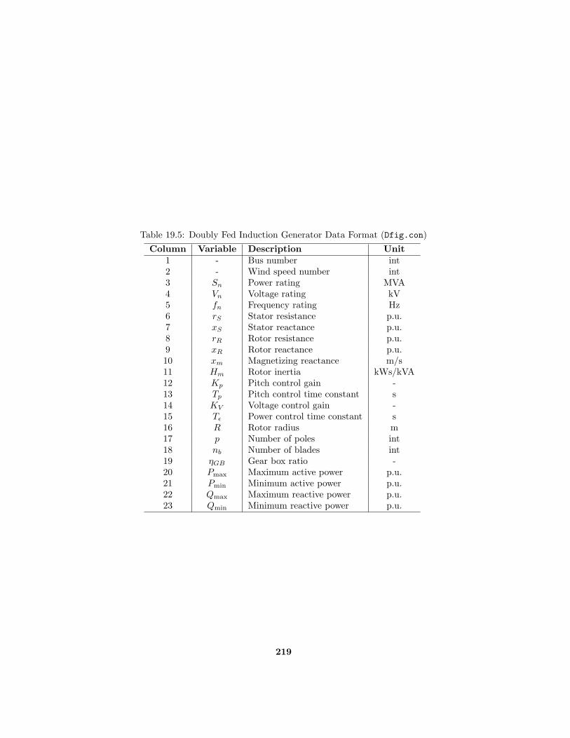
Table 19.5: Doubly Fed Induction Generator Data Format (Dfig.con)
Column Variable Description Unit1 - Bus number int2 - Wind speed number int3 Sn Power rating MVA4 Vn Voltage rating kV5 fn Frequency rating Hz6 rS Stator resistance p.u.7 xS Stator reactance p.u.8 rR Rotor resistance p.u.9 xR Rotor reactance p.u.10 xm Magnetizing reactance m/s11 Hm Rotor inertia kWs/kVA12 Kp Pitch control gain -13 Tp Pitch control time constant s14 KV Voltage control gain -15 Tε Power control time constant s16 R Rotor radius m17 p Number of poles int18 nb Number of blades int19 ηGB Gear box ratio -20 Pmax Maximum active power p.u.21 Pmin Minimum active power p.u.22 Qmax Maximum reactive power p.u.23 Qmin Minimum reactive power p.u.
219

220 19 Wind Turbines
Assuming a lossless converter and a power factor equal to 1, the output powers ofthe generator becomes:
Ps = Pc (19.45)
Qs = 0
Furthermore, the reactive power injected in the grid is controlled by means of theconverter direct current idc, which allows rewriting the second equation of (19.43),as follows:
Qc =1
cos(θ)V idc + tan(θ)Ps (19.46)
The generator motion equation is modeled as a single shaft, as it is assumedthat the converter controls are able to filter shaft dynamics. For the same reason,no tower shadow effect is considered in this model. Thus one has:
ωm = (Tm − Te)/2Hm (19.47)
Te = ψdsiqs − ψqsids
where the link between stator fluxes and generator currents is as follows:
ψds = −xdids + ψp (19.48)
ψqs = −xqiqs
The mechanical torque and power are modeled as in the doubly fed induction motor,thus equations from (19.34) to (19.37) apply.
Converter dynamics are highly simplified, as they are fast with respect to theelectromechanical transients. Thus, the converter is modeled as an ideal currentsource, where iqs, ids and idc are state variables and are used for the rotor speedcontrol and the reactive power control and the voltage control, respectively. Differ-ential equations of the converter currents are as follows:
iqs = (iqsref − iqs)/Tεp (19.49)
ids = (idsref − ids)/Tεq
idc = (KV (Vref − V ) − idc)/TV
where
iqsref =P ∗
w(ωm)
ωm(ψp − xdids)(19.50)
idsref =ψp
xd−
√ψ2
p
x2d
− Qref
ωmxd
where P ∗w(ωm) is the power-speed characteristic which roughly optimizes the
wind energy capture and which is calculated using the current rotor speed value(see Fig. 19.5). It is assumed that P ∗
w = 0 if the ωm < 0.5 p.u. and that P ∗w = 1 p.u.
if ωm > 1 p.u. Thus, the rotor speed control only has effect for sub-synchronous
19.2 Wind Turbines 221
speeds. Both the speed and voltage controls undergo anti-windup limiters in orderto avoid converter over-currents. Current limits are approximated as follows:
iqsmax= −Pmin (19.51)
iqsmin= −Pmax
idsmax= idcmax
= −Qmin
idsmin= idcmin
= −Qmax
Finally the pitch angle control is illustrated in Fig. 19.6 and described by thedifferential equation (19.40).
The wind turbine with direct drive synchronous generator is defined in the Ddsgstructure, which has the following fields:
1. con: direct drive synchronous generator data.
2. n: total number of direct drive synchronous generators.
3. bus: numbers of buses to which generators are connected.
4. wind: numbers of wind speed models to which generators are connected.
5. dat: generator parameters.
6. omega m: indexes of the state variable ωm.
7. theta p: indexes of the state variable θp.
8. ids: indexes of the state variable ids.
9. iqs: indexes of the state variable iqs.
10. idc: indexes of the state variable idc.
Table 19.5 depicts the data format of the wind turbine with direct drive synchronousgenerator.

Table 19.6: Direct Drive Synchronous Generator Data Format (Ddsg.con)
Column Variable Description Unit1 - Bus number int2 - Wind speed number int3 Sn Power rating MVA4 Vn Voltage rating kV5 fn Frequency rating Hz6 rs Stator resistance p.u.7 xd d-axis reactance p.u.8 xq q-axis reactance p.u.9 ψp Permanent field flux p.u.10 Hm Rotor inertia kWs/kVA11 Kp Pitch control gain -12 Tp Pitch control time constant s13 KV Voltage control gain -14 TV Voltage control time constant s15 Tεp Active power control time constant s16 Tεq Reactive power control time constant s17 R Rotor radius m18 p Number of poles int19 nb Number of blades int20 ηGB Gear box ratio -21 Pmax Maximum active power p.u.22 Pmin Minimum active power p.u.23 Qmax Maximum reactive power p.u.24 Qmin Minimum reactive power p.u.
222
Chapter 20
Other Models
This chapter describes additional components useful to represent particular dy-namic phenomena. These are synchronous machine dynamic shaft, sub-synchronousresonance generator model, solid oxide fuel cell, and sub-transmission equivalent ar-eas with load tap changer dynamics.
20.1 Dynamic Shaft
A dynamic mass-spring model is used for defining the shaft of the synchronousmachine. Figure 20.1 depicts the shaft scheme (springs are in solid black). Therotor mass is dashed since it is not actually part of the model. The dynamic shafthas to be connected to a synchronous machine.1
Table 20.1 depicts the dynamic shaft data format. The state variables areinitialized after solving the power flow, and a PV or a slack generator are requiredat the machine bus. A nominal frequency (ω = 1) is assumed when the shaft speedsare initialized. The power and frequency ratings of the shaft are inherited from thesynchronous machine associated with the shaft.
The complete set of differential equations which describe the dynamic shaft isas follows:
δHP
= Ωb(ωHP− 1) (20.1)
ωHP
= (Tm −DHP
(ωHP
− 1) −D12
(ωHP
− ωIP
)
+KHP
(δIP
− δHP
))/MHP
δIP
= Ωb(ωIP− 1)
ωIP
= (−DIP
(ωIP
− 1) −D12
(ωIP
− ωHP
) −D23
(ωIP
− ωLP
)
+KHP
(δHP
− δIP
) +KIP
(δLP
− δIP
))/MIP
δLP
= Ωb(ωLP− 1)
ωLP
= (−DLP
(ωLP
− 1) −D23
(ωLP
− ωIP
) −D34
(ωLP
− ω)
1In the current PSAT version, turbine governors cannot be connected to the shaft.
223

224 20 Other Models
PSfrag replacements
Tm Te
HP IP LP EXrotor
Figure 20.1: Synchronous machine mass-spring shaft model.
+KIP
(δIP
− δLP
) +KLP
(δ − δLP
))/MLP
δ = Ωb(ω − 1)
ω = (−Te −D(ω − 1) −D34
(ω − ωLP
) −D45
(ω − ωEX
)
+KLP
(δLP
− δ) +KEX
(δEX
− δ))/M
δEX
= Ωb(ωEX− 1)
ωEX
= (−DEX
(ωEX
− 1) −D45
(ωEX
− ω)
+KEX
(δ − δEX
))/MEX
Dynamic shafts are defined in the structure Mass, as follow:
1. con: data of the Mass components.
2. syn: indexes of generators to which the shafts are connected.
3. n: total number of dynamic shafts.
4. delta HP: indexes of the state variable δHP
.
5. omega HP: indexes of the state variable ωHP
.
6. delta IP: indexes of the state variable δIP
.
7. omega IP: indexes of the state variable ωIP
.
8. delta LP: indexes of the state variable δLP
.
9. omega LP: indexes of the state variable ωLP
.
10. delta EX: indexes of the state variable δEX
.
11. omega EX: indexes of the state variable ωEX
.

20.2 Sub-synchronous Resonance Model 225
Table 20.1: Dynamic Shaft Data Format (Mass.con)
Column Variable Description Unit1 - Synchronous machine number int2 M
HPHigh pressure turbine inertia kWs/kVA
3 MIP
Intermediate pressure turbine inertia kWs/kVA4 M
LPLow pressure turbine inertia kWs/kVA
5 MEX
Exciter inertia kWs/kVA6 D
HPHigh pressure turbine damping p.u.
7 DIP
Intermediate pressure turbine damping p.u.8 D
LPLow pressure turbine damping p.u.
9 DEX
Exciter damping p.u.10 D
12High-Interm. pressure turbine damping p.u.
11 D23
Interm.-low pressure turbine damping p.u.12 D
34Low pressure turbine-rotor damping p.u.
13 D45
Rotor-exciter damping p.u.14 K
HPHigh pressure turbine angle coeff. p.u.
15 KIP
Intermed. pressure turbine angle coeff. p.u.16 K
LPLow pressure turbine angle coeff. p.u.
17 KEX
Exciter angle coefficient p.u.
20.2 Sub-synchronous Resonance Model
Figure 20.2 depicts a generator with shaft dynamics and compensated line, whichrepresents a simple model for studying the sub-synchronous resonance (SSR) prob-lem. The shaft dynamics are similar to what described in Section 20.1 and aremodeled as high, intermediate and low pressure turbine masses, exciter mass andmachine rotor.
This is one of the simplest models [Yao-Nan-Yu 1983] which presents the sub-synchronous resonance (SSR) phenomenon, a well known problem of undampedoscillations that may occur when the transmission line to which the machine isconnected is compensated by a series capacitor [Force 1977, Report 1985, Report1992].
The dynamics of the RLC circuit cannot be neglected since the line presents twomodes whose frequency can be roughly estimated as Ωb(1±
√xC/xL). For typical
values of the inductive and capacitive reactances, the lower of these two frequenciescan be close to one of the mechanical oscillations of the generator shaft. Thus,beyond a certain value of the compensation level, the machine may experiment anegative damping of one of the mechanical modes that results in dangerous stresseson the shaft. This phenomenon can be also described in terms of the bifurcationtheory [Mitani and Tsuji 1995, Mitani et al. 1998].
The model used for representing the machine and the line is the same usedin [Zhu et al. 1996]. It presents five electrical state variables (id, iq, if , vdc
, vqc)
which can be determined by the machine differential equations:

226 20 Other ModelsPSfrag replacements
r xL xC
vd + jvqvdC
+ jvqC
V ∠θ
id + jiq
Tm Te
HP IP LP EXδ, ω
Figure 20.2: Generator with dynamic shaft and compensated line.
ψf = (vfd − if )/T ′d0 (20.2)
ψd = Ωb(raid + ωψq + vd)
ψq = Ωb(raiq − ωψd + vq)
the line differential equations:
id = Ωb(iq + (vd − rid − vdc− V sin(δ − θ))/xL) (20.3)
iq = Ωb(−id + (vq − riq − vqc− V cos(δ − θ))/xL)
vdc= Ωb(xCid + vqc
)
vqc= Ωb(xCiq − vdc
)
along with the algebraic constraints that link the time derivatives of the generatorfluxes and of the line currents:
ψf = if − (xd − x′d)id (20.4)
ψd = if − xdid
ψq = −xq iq

20.2 Sub-synchronous Resonance Model 227
Finally, a five mass system is used for describing the shaft dynamics:
δHP
= Ωb(ωHP− 1) (20.5)
ωHP
= (Tm −DHP
(ωHP
− 1) +KHP
(δIP
− δHP
))/MHP
δIP
= Ωb(ωIP− 1)
ωIP
= (−DIP
(ωIP
− 1) +KHP
(δHP
− δIP
)
+KIP
(δLP
− δIP
))/MIP
δLP
= Ωb(ωLP− 1)
ωLP
= (−DLP
(ωLP
− 1) +KIP
(δIP
− δLP
)
+KLP
(δ − δLP
))/MLP
δ = Ωb(ω − 1)
ω = (−Te −D(ω − 1) +KLP
(δLP
− δ)
+KEX
(δEX
− δ))/M
δEX
= Ωb(ωEX− 1)
ωEX
= (−DEX
(ωEX
− 1) +KEX
(δ − δEX
))/MEX
where the electrical torque is Te = ψdiq − ψqid. The algebraic equations for thepower injections
P = −V id sin(δ − θ) − V iq cos(δ − θ) (20.6)
Q = −V id cos(δ − θ) + V iq sin(δ − θ)
complete the model. In the implemented code, the field reactance xf , the fieldresistance rf and the d-axis reactance xad are used instead of x′d and T ′
d0, with thefollowing relationships:
T ′d0 =
xf
Ωbrf(20.7)
x′d = xd − xad
The sub-synchronous resonance generator model is defined in the structure SSR,as follows:
1. con: SSR data.
2. bus: indexes of buses to which SSRs are connected.
3. n: total number of SSRs.
4. Id: indexes of the state variable id.
5. Iq: indexes of the state variable iq .
6. If: indexes of the state variable if .
7. Edc: indexes of the state variable vdc.
228 20 Other Models
8. Eqc: indexes of the state variable vqc.
9. Tm: mechanical torque Tm.
10. Efd: field voltage vfd.
11. delta HP: indexes of the state variable δHP
.
12. omega HP: indexes of the state variable ωHP
.
13. delta IP: indexes of the state variable δIP
.
14. omega IP: indexes of the state variable ωIP
.
15. delta LP: indexes of the state variable δLP
.
16. omega LP: indexes of the state variable ωLP
.
17. delta: indexes of the state variable δ.
18. omega: indexes of the state variable ω.
19. delta EX: indexes of the state variable δEX
.
20. omega EX: indexes of the state variable ωEX
.
The SSR data format is depicted in Table 20.2. The SSR state variables areinitialized after solving the power flow and either a PV or a slack generator isneeded at the SSR bus.
20.3 Solid Oxide Fuel Cell
A Solid Oxide Fuel Cell (SOFC) model is included in PSAT based on what wasproposed in [Padulles et al. 2000], [Zhu and Tomsovic 2002], [Hatziadoniu et al.2002], and [Knyazkin et al. 2003].2 Figure 20.3 depicts the fuel cell scheme, whichis based on the following equations:
pH2= ((qH2
− 2KrIk)/KH2− pH2
)/τH2(20.8)
pH2O = (2KrIk/KH2O − pH2O)/τH2O
pO2= ((qH2
/rHO −KrIk)/kO2− pO2
)/τO2
qH2= (2KrIk/Uopt − qH2
)/Tf
Vk = (−Vk − rIk +N0(E0 +RT
2Fln(pH2
√pO2
/pH2O)))/Tε
where R is the gas constant (R = 8.314 [J/(mol K)]), F is the Faraday constant(F = 96487 [C/mol]), T the absolute gas temperature, and Tε is a “small” time
2This model was realized in collaboration with Valery Knyazkin, Ph.D. candidate at the RoyalInstitute of Technology, Sweden.

Table 20.2: SSR Data Format (SSR.con)
Column Variable Description Unit1 - Bus number int2 Sn Power rating MVA3 Vn Voltage rating kV4 fn Frequency rating Hz5 xd d-axis synchronous reactance p.u.6 xq q-axis synchronous reactance p.u.7 ra Armature resistance p.u.8 xad d-axis reactance p.u.9 r Line resistance p.u.10 xL Line inductive reactance p.u.11 xC Line capacitive reactance p.u.12 rf Field resistance p.u.13 xf Field reactance p.u.14 M
HPHigh pressure turbine inertia kWs/kVA
15 MIP
Intermediate pressure turbine inertia kWs/kVA16 M
LPLow pressure turbine inertia kWs/kVA
17 M Rotor inertia kWs/kVA18 M
EXExciter inertia kWs/kVA
19 DHP
High pressure turbine damping p.u.20 D
IPIntermediate pressure turbine damping p.u.
21 DLP
Low pressure turbine damping p.u.22 D Rotor damping p.u.23 D
EXExciter damping p.u.
24 KHP
High pressure turbine angle coeff. p.u.25 K
IPIntermed. pressure turbine angle coeff. p.u.
26 KLP
Low pressure turbine angle coeff. p.u.27 K
EXExciter angle coefficient p.u.
229

230 20 Other Models
constant which does not affects the fuel cell dynamics. The fuel cell current Ik canbe subjected to a constant power control:
Ik = (Pref/Vk − Ik)/Te (20.9)
or a constant current control:
Ik = (Pref/V(k0) − Ik)/Te (20.10)
where Vk0is the initial fuel cell DC voltage. If the input signal exceeds the dynamic
limits proportional to the fuel flow, one has:
Ik = (UlimqH2
2Kr− Ik)/Te (20.11)
where Ulim is the maximum or the minimum fuel utilization (Umax, Umin). Theconnection with the network is assumed to be realized by means of an ideal inverterand a transformer with reactance xT , as depicted in Fig. 20.4. The AC voltage isregulated by means of the inverter modulating amplitude m, as follows:
m = (Km(Vref − Vs) −m)/Tm (20.12)
The amplitude control has anti-windup limiters and is depicted in Fig. 20.5.The DC power of the fuel cell (Pk = VkIk) is considered to be the real power
injected in the network (Ps = Pk). Thus the link with the AC network is as follows:
Ps =VtVs
xTsin(θt − θs) = VkIk (20.13)
Qs =VtVs
xTcos(θt − θs) −
V 2s
xT
where Vt = kmVk, k =√
3/8. Thus, one has:
θt = θs + asin
(xT IkkmVs
)(20.14)
and, finally:
Qs = −V2s
xT+VskmVk
xT
√
(1 −(xT IkkmVs
)2
(20.15)
The reference voltage Vref and the initial value of the inverter amplitude m0 arecomputed based on the power flow solution, as follows:
m0 =xt
VskVk
√
P 2g +
(Qg +
V 2g
xT
)2
(20.16)
Vref = Vg +m/Km
where Vg, Pg and Qg are the PV generator voltage, active power and reactivepower respectively. Observe that to be properly initialized, the fuel cell needs a PVgenerator connected at the same bus (slack generators are not allowed).
The SOFC model is defined in the structure Sofc, as follows:

_
_
_
PSfr
agre
pla
cem
ents
1
11
+
+
+
−
rK
r
2Kr
2Kr
Pref
I k
I k
Vk
Pk
1/V
k
q H2
q H2
q H2
q O2
pH
2p
O2
pH
2O
pH
2O
r HO
Uopt
Um
ax/2K
r
Um
in/2K
r
pH
2
√p
O2
1/K
H2
τ H2s
+1
1/K
H2O
τ H2Os
+1
1/K
O2
τ O2s
+1
Tfs
+1
Tes
+1
N0
E0+
lnRT
2F
Figure 20.3: Solid Oxide Fuel Cell scheme.
231

Table 20.3: Solid Oxide Fuel Cell Data Format (Sofc.con)
Column Variable Description Unit1 - Bus number int2 Sn Power rating MW3 Vn Voltage rating kV4 Te Electrical response time s5 τH2
Response time for hydrogen flow s6 KH2
Valve molar constant for hydrogen -7 Kr Constant -8 τH2O Response time for water flow s9 KH2O Valve molar constant for water -10 τO2
Response time for oxygen flow s11 KO2
Valve molar constant for oxygen -12 rHO Ratio of hydrogen to oxygen -13 Tf Fuel processor response time s14 Uopt Optimal fuel utilization -15 Umax Maximum fuel utilization -16 Umin Minimum fuel utilization -17 r Ohmic losses Ω18 N0 Number of cells in series in the stack p.u.19 E0 Ideal standard potential V20 T Gas Absolute temperature K† 21 Pref Reference power p.u.† 22 Vref Reference AC voltage p.u.† 23 PB Base power MW† 24 VB Base voltage kV25 - Control mode (1) current, (0) power int26 xT Transformer reactance p.u.27 Km Gain of the voltage control loop p.u.28 Tm Time constant of the voltage control loop s29 mmax Maximum modulating amplitude p.u./p.u.30 mmin Minimum modulating amplitude p.u./p.u.
Note: fields marked with a † are not set by the user.
232

20.4 Sub-tramsmission Area Equivalents 233
PSfrag replacements
Vk
Vt∠θt Vs∠θs
Ik
Figure 20.4: Solid Oxide Fuel Cell connection with the AC grid.
−
+
PSfrag replacements
Vref
Vs m
mmax
mmin
Km
Tms+ 1
Figure 20.5: AC voltage control for the Solid Oxide Fuel Cell.
1. con: Solid Oxide Fuel Cell data.
2. bus: indexes of buses to which SOFCs are connected.
3. n: total number of SOFCs.
4. Ik: indexes of the state variable Idc.
5. Vk: indexes of the state variable Vdc .
6. pH2: indexes of the state variable pH2.
7. pH2O: indexes of the state variable pH2O.
8. pO2: indexes of the state variable pO2.
9. qH2: indexes of the state variable qH2.
10. m: indexes of the state variable m.
20.4 Sub-tramsmission Area Equivalents
Three sub-transmission area equivalent (SAE) models are included in PSAT basedon what was proposed in [Denegri et al. 2001]. A SAE with three LTCs and loads

234 20 Other Models
is depicted 20.6.a. Each load is considered to be static and voltage dependent, asfollows:
PLi= βi
Vi
mi(20.17)
QLi= αi
V 2i
m2i
where mi is the tap ratio of the LTC connected to the load i. The LTC controlsthe load voltage and the following differential equation holds:
mi = −himi + ki(Vi
mi− Vrefi) (20.18)
Generic algebraic equations of the SAE are obtained by means of a “nodal” re-duction of the network which is described in [Denegri et al. 2001] and can besummarized as follows:
PA =x∗
xA0
( N∑
i=1
kPi
)VA +
x∗
xA0xB0VAVB sin(θA − θB) (20.19)
QA =
(1
xA0− x∗
x2A0
)V 2
A − x∗
xA0xB0VAVB cos(θA − θB)
PB =x∗
xB0
( N∑
i=1
kPi
)VB +
x∗
xA0xB0VAVB sin(θB − θA)
QB =
(1
xB0− x∗
x2B0
)V 2
B − x∗
xA0xB0VAVB cos(θB − θA)
where
bA = − 1
xA0
[1 − x∗
(1
xA0+
1
xB0
)](20.20)
bB = − 1
xB0
[1 − x∗
(1
xB0+
1
xA0
)]
bAB = − x∗
xB0xA0
IA =x∗
xA0
N∑
i=1
kPi
IB =x∗
xB0
N∑
i=1
kPi
x∗ =
(1
xA0+
1
xB0+
N∑
i=1
kQi
)−1

20.4 Sub-tramsmission Area Equivalents 235
and
kPi=
βi
mix0i
(1
x0i+αi
m2i
)−1
(20.21)
kPi=
1
x0i− 1
x20i
(1
x0i+αi
m2i
)−1
The meaning of the variables is illustrated in Fig. 20.6, which depicts the nodalreduction procedure. A “modal” reduction is also proposed in [Denegri et al. 2001],based on the assumption of dynamic coherence of LTCs, as follows:
meq =1
N
N∑
i=1
fi(meq) (20.22)
where N is the total number of LTC and loads, and fi is:
fi(mi) = mi (20.23)
= −himi + ki
(x∗
(VA
xA0+
VB
xB0
)(xTi
mi
(1
xTi
+αi
m2i
)− Vrefi
)−1)
Three SAE models are implemented:
1. SAE with three LTCs and loads, modal and nodal reductions defined in thestructure SAE1 as follows:
con SAE datan total number of SAEm indexes of state variables meq
2. SAE with two LTCs and loads and nodal reductions defined in the structureSAE2 as follows:
con SAE datan total number of SAEm1 indexes of state variables m1
m2 indexes of state variables m2
3. SAE with three LTCs and loads and modal reductions defined in the structureSAE3 as follows:
con SAE datan total number of SAEm1 indexes of state variables m1
m2 indexes of state variables m2
m3 indexes of state variables m3
The SAE data format are depicted in Tables 20.4 and 20.5. Parameters markedwith ‡ are computed at the initialization step if parameters marked with a † areprovided.
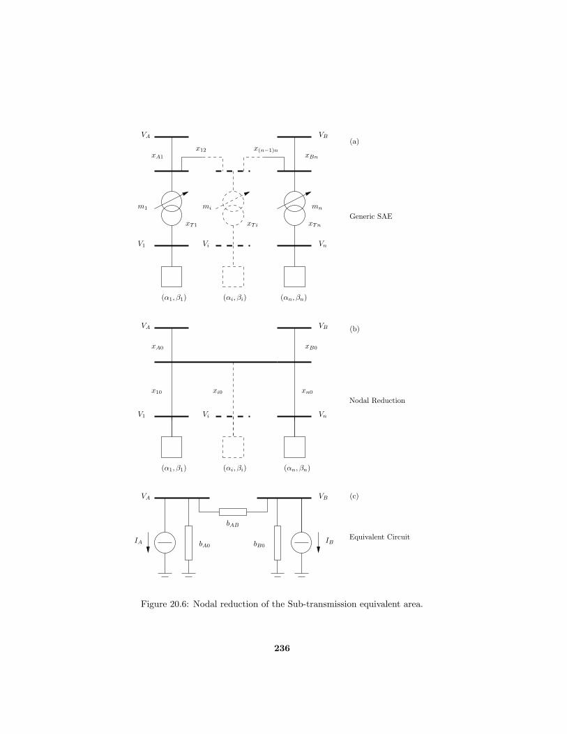
PSfrag replacements
(a)
(b)
(c)
Generic SAE
Nodal Reduction
Equivalent Circuit
V1
V1
Vi
Vi
Vn
Vn
VA
VA
VA
VB
VB
VB
IA IB
xA0 xB0
x10 xi0 xn0
xT1 xTi xTn
xA1
x12 x(n−1)nxBn
m1 mi mn
(α1, β1)
(α1, β1) (αi, βi)
(αi, βi) (αn, βn)
(αn, βn)
bAB
bA0 bB0
Figure 20.6: Nodal reduction of the Sub-transmission equivalent area.
236
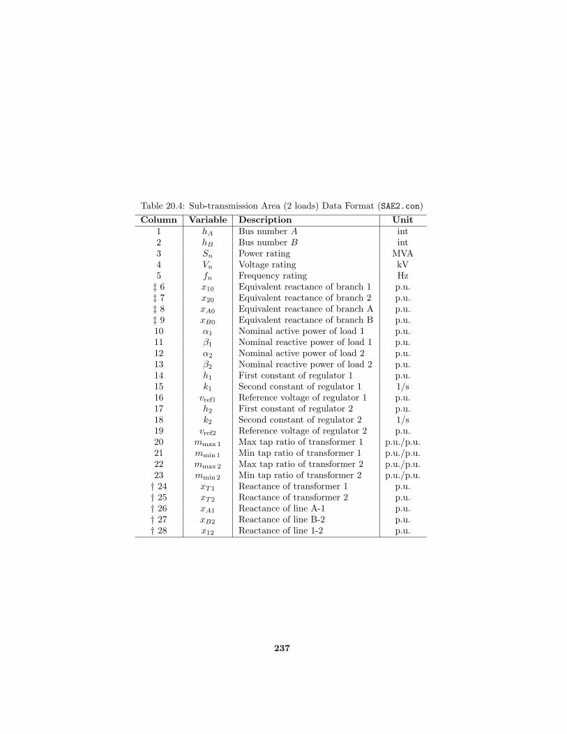
Table 20.4: Sub-transmission Area (2 loads) Data Format (SAE2.con)
Column Variable Description Unit1 hA Bus number A int2 hB Bus number B int3 Sn Power rating MVA4 Vn Voltage rating kV5 fn Frequency rating Hz‡ 6 x10 Equivalent reactance of branch 1 p.u.‡ 7 x20 Equivalent reactance of branch 2 p.u.‡ 8 xA0 Equivalent reactance of branch A p.u.‡ 9 xB0 Equivalent reactance of branch B p.u.10 α1 Nominal active power of load 1 p.u.11 β1 Nominal reactive power of load 1 p.u.12 α2 Nominal active power of load 2 p.u.13 β2 Nominal reactive power of load 2 p.u.14 h1 First constant of regulator 1 p.u.15 k1 Second constant of regulator 1 1/s16 vref1 Reference voltage of regulator 1 p.u.17 h2 First constant of regulator 2 p.u.18 k2 Second constant of regulator 2 1/s19 vref2 Reference voltage of regulator 2 p.u.20 mmax 1 Max tap ratio of transformer 1 p.u./p.u.21 mmin 1 Min tap ratio of transformer 1 p.u./p.u.22 mmax 2 Max tap ratio of transformer 2 p.u./p.u.23 mmin 2 Min tap ratio of transformer 2 p.u./p.u.† 24 xT1 Reactance of transformer 1 p.u.† 25 xT2 Reactance of transformer 2 p.u.† 26 xA1 Reactance of line A-1 p.u.† 27 xB2 Reactance of line B-2 p.u.† 28 x12 Reactance of line 1-2 p.u.
237

Table 20.5: Sub-transmission Area (3 loads) Data Format (SAE1.con, SAE3.con)
Column Variable Description Unit1 hA Bus number A int2 hB Bus number B int3 Sn Power rating MVA4 Vn Voltage rating kV5 fn Frequency rating Hz‡ 6 x10 Equivalent reactance of branch 1 p.u.‡ 7 x20 Equivalent reactance of branch 2 p.u.‡ 8 x30 Equivalent reactance of branch 3 p.u.‡ 9 xA0 Equivalent reactance of branch A p.u.‡10 xB0 Equivalent reactance of branch B p.u.11 α1 Nominal active power of load 1 p.u.12 β1 Nominal reactive power of load 1 p.u.13 α2 Nominal active power of load 2 p.u.14 β2 Nominal reactive power of load 2 p.u.15 α3 Nominal active power of load 3 p.u.16 β3 Nominal reactive power of load 3 p.u.17 h1 First constant of regulator 1 p.u.18 k1 Second constant of regulator 1 1/s19 vref1 Reference voltage of regulator 1 p.u.20 h2 First constant of regulator 2 p.u.21 k2 Second constant of regulator 2 1/s22 vref2 Reference voltage of regulator 2 p.u.23 h3 First constant of regulator 3 p.u.24 k3 Second constant of regulator 3 1/s25 vref3 Reference voltage of regulator 3 p.u.26 mmax 1 Max tap ratio of transformer 1 p.u./p.u.27 mmin 1 Min tap ratio of transformer 1 p.u./p.u.28 mmax 2 Max tap ratio of transformer 2 p.u./p.u.29 mmin 2 Min tap ratio of transformer 2 p.u./p.u.30 mmax 3 Max tap ratio of transformer 3 p.u./p.u.31 mmin 3 Min tap ratio of transformer 3 p.u./p.u.† 32 xT1 Reactance of transformer 1 p.u.† 33 xT2 Reactance of transformer 2 p.u.† 34 xT3 Reactance of transformer 3 p.u.† 35 xA1 Reactance of line A-1 p.u.† 36 xB2 Reactance of line B-2 p.u.† 37 x12 Reactance of line 1-2 p.u.† 38 x23 Reactance of line 2-3 p.u.
238