Manual versus Automatic Parallelization Using PVM and HPF

MANUAL VERSUS AUTOMATIC PARALLELIZATION

USING PVM AND HPF

by

Hongyi Hu

A project

submitted in partial fulfillment

of the requirements for the degree of

Master of Science in Computer Science

Boise State University

November 2004

c© 2004Hongyi Hu

ALL RIGHTS RESERVED

The project presented by Hongyi Hu entitledManual versus Automatic Parallelization

Using PVM and HPF is hereby approved.

Amit Jain, Advisor Date

John Griffin, Committee Member Date

Jyh-Haw Yeh, Committee Member Date

John R. Pelton, Graduate Dean Date

dedicated to Hao and Erica

iv

ACKNOWLEDGEMENTS

I would like to thank my family for all of their support through the years. I would

never have gotten where I am today without them.

I would also like to thank my advisor, Dr. Amit Jain, who taught me how impor-

tant parallel programming techniques are for solving large computational problems.

His parallel programming class spurred my interest in exploring the performance of

different parallel programming languages.

I also thank the other members of my committee, Dr. John Griffin and Dr. Jyh-

Haw Yeh, for all their help with this project, particularly with the writing of the final

report.

I thank Dr.Jodi Mead, Dr.Partha Routh and Dr. Barbara Zubik-Kowal for their

time and effort with helping me to understand their program and search the compu-

tational block for parallelization.

Finally, I would like to thank all my friends for the encouragement that helped

me complete this endeavor.

This material is based upon work supported by the National Science Foundation

under Grant No. 0321233. Any opinions, findings, and conclusions or recommenda-

tions expressed in this material are those of the author and do not necessarily reflect

the views of the National Science Foundation.

v

ABSTRACT

The use of multiple computers/processors can lead to substantial speedups on

large computational problems. However there is a significant barrier of converting se-

quential code to run in parallel. Several parallel programming languages and libraries

have been developed to ease the task of writing programs for multiple-processors.

One approach is to add calls to a parallel library in the sequential code. This man-

ual parallelization is considered to require more expertise. Parallel Virtual Machine

(PVM) and Message Passing Interface (MPI) are the two most well-known parallel

programming libraries. PVM was used as the library in this project.

At the other end of the spectrum is automatic parallelization. High Performance

Fortran (HPF) is a widely used example. In automatic parallelization, the user pro-

vides directives that guide the compiler in automatically parallelizing the code. HPF

is seen as requiring less expertise.

The goal of this project was to quantitatively and qualitatively evaluate manual

versus automatic parallelization using three actual research codes. The three serial

codes are from the areas of Waveform Relaxation, Ocean Currents Simulation in

Mathematics and Data Inversion for Earth Model in Geophysics. The codes were

analyzed and were determined to have substantial parallelism that seemed relatively

easy to exploit. The experiment went through the process of converting the three

vi

sequential codes into PVM and HPF, running parallel codes on a 60-node Beowulf

Cluster, and comparing performance results.

In two out of three programs, HPF provided a comparable speedup to manual

parallelization with PVM. However in the third code, HPF provided a speedup that

was an order of magnitude less than with PVM. Surprisingly, considerable effort

was required to get HPF to perform well. In fact, the effort required for manual

parallelization was not substantially more in two out of three cases.

vii

TABLE OF CONTENTS

LIST OF TABLES . . . . . . . . . . . . . . . . . . . . . . . . . . . . . . . xii

LIST OF FIGURES . . . . . . . . . . . . . . . . . . . . . . . . . . . . . . xiii

1 INTRODUCTION . . . . . . . . . . . . . . . . . . . . . . . . . . . . . 1

1.1 Rationale and Significance . . . . . . . . . . . . . . . . . . . . . . . . 1

1.2 Background about PVM . . . . . . . . . . . . . . . . . . . . . . . . . 2

1.3 Background about HPF . . . . . . . . . . . . . . . . . . . . . . . . . 3

1.3.1 PGHPF . . . . . . . . . . . . . . . . . . . . . . . . . . . . . . 4

1.4 Background on Beowulf Cluster . . . . . . . . . . . . . . . . . . . . . 5

1.5 Problem Statement . . . . . . . . . . . . . . . . . . . . . . . . . . . . 6

1.6 Three sequential FORTRAN Programs . . . . . . . . . . . . . . . . . 6

2 THE APPLICATION CODES . . . . . . . . . . . . . . . . . . . . . . 8

2.1 Wave Relaxation Schemes (WRS) Code . . . . . . . . . . . . . . . . . 8

2.2 Ocean Currents Simulation (OCS) Code . . . . . . . . . . . . . . . . 10

2.3 Inversion of Controlled Source Audio-Frequency Magnetotelluric Data(ICSAMD) Code . . . . . . . . . . . . . . . . . . . . . . . . . . . . . 13

3 PARALLELIZING APPLICATIONS IN PVM . . . . . . . . . . . 16

3.1 Rewriting Wave Relaxation Schemes (WRS) Code . . . . . . . . . . . 19

3.1.1 Analysis . . . . . . . . . . . . . . . . . . . . . . . . . . . . . . 19

3.1.2 PVM Implementation on WRS Code . . . . . . . . . . . . . . 22

viii

3.2 Rewriting Ocean Currents Simulation (OCS) Code . . . . . . . . . . 23

3.2.1 Analysis . . . . . . . . . . . . . . . . . . . . . . . . . . . . . . 23

3.2.2 PVM Implementation on OCS Code . . . . . . . . . . . . . . 27

3.3 Rewriting Inversion of Controlled Source Audio-Frequency Magnetotel-luric Data (ICSAMD) Code . . . . . . . . . . . . . . . . . . . . . . . 27

3.3.1 Analysis . . . . . . . . . . . . . . . . . . . . . . . . . . . . . . 27

3.3.2 PVM Implementation on ICSAMD Code . . . . . . . . . . . . 30

4 PARALLELIZING APPLICATIONS IN HPF . . . . . . . . . . . 33

4.1 Rewriting Wave Relaxation Schemes (WRS) Code . . . . . . . . . . 33

4.1.1 Analysis . . . . . . . . . . . . . . . . . . . . . . . . . . . . . . 33

4.1.2 The HPF implementation on WRS Code . . . . . . . . . . . . 35

4.2 Rewriting Ocean Currents Simulation (OCS) Code . . . . . . . . . . 35

4.2.1 Analysis . . . . . . . . . . . . . . . . . . . . . . . . . . . . . . 35

4.2.2 The HPF implementation on OCS Code . . . . . . . . . . . . 36

4.3 Rewriting Inversion of Controlled Source Audio-Frequency Magne-totelluric Data (ICSAMD) Code . . . . . . . . . . . . . . . . . . . . . 37

4.3.1 Analysis . . . . . . . . . . . . . . . . . . . . . . . . . . . . . . 37

4.3.2 The HPF implementation on ICSAMD Code . . . . . . . . . . 39

5 COMPARISON OF RUNNING SPEED BETWEEN THE PAR-ALLEL IMPLEMENTATIONS IN PVM VERSUS IN HPF . . . 41

5.1 The Experiment Result for the WRS Code . . . . . . . . . . . . . . . 41

5.2 The Experiment Result for the OCS Code . . . . . . . . . . . . . . . 43

5.3 The Experiment Result for the ICSAMD Code . . . . . . . . . . . . . 44

5.4 The Experiment Discussion . . . . . . . . . . . . . . . . . . . . . . . 45

ix

6 CONCLUSIONS . . . . . . . . . . . . . . . . . . . . . . . . . . . . . . 46

6.1 Summary and Conclusions . . . . . . . . . . . . . . . . . . . . . . . . 46

REFERENCES . . . . . . . . . . . . . . . . . . . . . . . . . . . . . . . . . 48

APPENDIX A THE SKETCH CODES IN CHAPTER 2 . . . . . . 50

A.1 Sketch Code: the Quadruply-Nested Iterations in the Sequential WRSCode in FORTRAN 90 . . . . . . . . . . . . . . . . . . . . . . . . . . 50

A.2 Sketch Code: the Doubly-Nested Loops in the Sequential OCS Codein FORTRAN 90 . . . . . . . . . . . . . . . . . . . . . . . . . . . . . 51

A.3 Sketch Code: the Single Loop in Subroutine data input in the Sequen-tial ICSAMD Code in FORTRAN 77 . . . . . . . . . . . . . . . . . . 52

APPENDIX B PVM IMPLEMENTATIONS IN CHAPTER 3 . . . 54

B.1 PVM Implementation on WRS Code . . . . . . . . . . . . . . . . . . 54

B.1.1 The Makefile.aimk of PVM WRS Code . . . . . . . . . . . . . 54

B.1.2 The WRS Sketch Code in PVM with Slow Speed . . . . . . . 55

B.1.3 The WRS Sketch Code in PVM with Fast Speed . . . . . . . . 58

B.2 PVM Implementation on OCS Code . . . . . . . . . . . . . . . . . . 59

B.2.1 The Makefile.aimk of PVM OCS Code . . . . . . . . . . . . . 59

B.2.2 The OCS Sketch Code in PVM . . . . . . . . . . . . . . . . . 61

B.3 PVM Implementation on ICSAMD Code . . . . . . . . . . . . . . . . 64

B.3.1 The Makefile.aimk of PVM ICSAMD Code . . . . . . . . . . . 64

B.3.2 The ICSAMD Sketch Code in PVM . . . . . . . . . . . . . . . 67

APPENDIX C HPF IMPLEMENTATIONS IN CHAPTER 4 . . . 76

C.1 HPF Implementation on WRS Code . . . . . . . . . . . . . . . . . . 76

C.1.1 The Makefile of HPF WRS Code . . . . . . . . . . . . . . . . 76

x

C.1.2 The Sketch Code of HPF WRS Code . . . . . . . . . . . . . . 76

C.2 HPF Implementation on OCS Code . . . . . . . . . . . . . . . . . . . 77

C.2.1 The Makefile of HPF OCS Code . . . . . . . . . . . . . . . . . 77

C.2.2 The Sketch Code of HPF OCS Code . . . . . . . . . . . . . . 78

C.3 HPF Implementation on ICSAMD Code . . . . . . . . . . . . . . . . 80

C.3.1 The Makefile of HPF ICSAMD Code . . . . . . . . . . . . . . 80

C.3.2 The Sketch Code of HPF ICSAMD Code . . . . . . . . . . . . 82

xi

LIST OF TABLES

3.1 Speed Comparison between the Slow PVM Version and the Fast PVMVersion . . . . . . . . . . . . . . . . . . . . . . . . . . . . . . . . . . . 22

5.1 The Runtime of the PVM WRS Code and the HPF WRS Code withthe Second Inner Loop Parallelized . . . . . . . . . . . . . . . . . . . 42

5.2 The Speedup of the PVM WRS Code and the HPF WRS Code . . . 435.3 The Runtime of the HPF WRS Code with the Third Inner Loop Par-

allelized . . . . . . . . . . . . . . . . . . . . . . . . . . . . . . . . . . 435.4 The Runtime of the PVM OCS Code and the HPF OCS Code . . . . 445.5 The Speedup of the PVM OCS Code and the HPF OCS Code . . . . 445.6 The Runtime of the PVM ICSAMD Code and the HPF ICSAMD Code 445.7 The Speedup of the PVM ICSAMD Code and the HPF ICSAMD Code 45

6.1 The Approximate Time of Parallelizing Each Code . . . . . . . . . . 46

xii

LIST OF FIGURES

2.1 The Structure of the Quadruply-Nested Iterations . . . . . . . . . . . 92.2 The Structure of the Doubly-Nested Iterations . . . . . . . . . . . . . 112.3 The Flow Chart of Subroutine Calls for OCS Code . . . . . . . . . . 122.4 The Flow Chart of Subroutine Calls for ICSAMD Code . . . . . . . . 142.5 The Structure of the Loop in Subroutine data input . . . . . . . . . . 15

3.1 SPMD Computational Model . . . . . . . . . . . . . . . . . . . . . . 173.2 MPMD Computational Model . . . . . . . . . . . . . . . . . . . . . . 183.3 The Master-Slave Approach of SPMD Computational Model . . . . . 193.4 The Data Partition and Collection of One Column of the Matrix . . . 213.5 The Data Partition and Collection of a Share of Rows of the Matrix . 233.6 The Master-Slave Approach of SPMD Computational Model in WRS

Code . . . . . . . . . . . . . . . . . . . . . . . . . . . . . . . . . . . . 243.7 The Real Time Performance Snapshot of PVM WRS . . . . . . . . . 253.8 The Data Partition and Collection of the Matrix Calculation . . . . . 263.9 The Real Time Performance Snapshot of PVM OCS . . . . . . . . . 283.10 Work Pool Approach . . . . . . . . . . . . . . . . . . . . . . . . . . . 293.11 The Real Time Performance Snapshot of PVM ICSAMD . . . . . . . 32

xiii

Chapter 1

INTRODUCTION

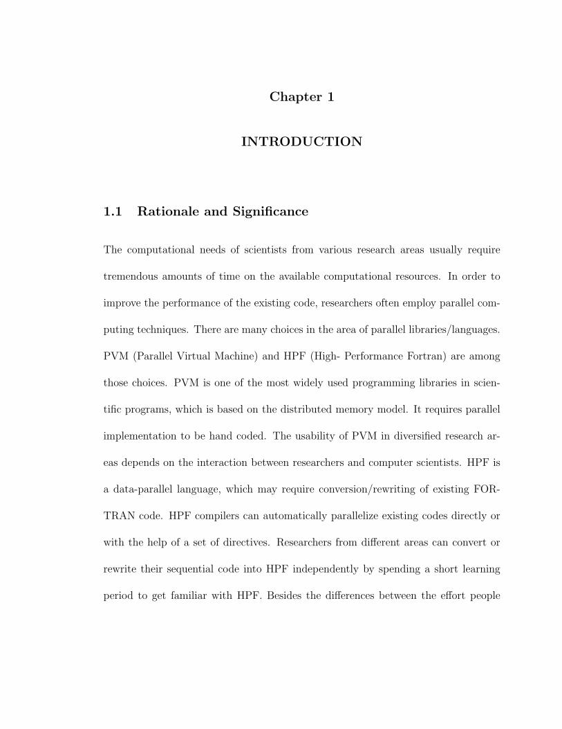
1.1 Rationale and Significance

The computational needs of scientists from various research areas usually require

tremendous amounts of time on the available computational resources. In order to

improve the performance of the existing code, researchers often employ parallel com-

puting techniques. There are many choices in the area of parallel libraries/languages.

PVM (Parallel Virtual Machine) and HPF (High- Performance Fortran) are among

those choices. PVM is one of the most widely used programming libraries in scien-

tific programs, which is based on the distributed memory model. It requires parallel

implementation to be hand coded. The usability of PVM in diversified research ar-

eas depends on the interaction between researchers and computer scientists. HPF is

a data-parallel language, which may require conversion/rewriting of existing FOR-

TRAN code. HPF compilers can automatically parallelize existing codes directly or

with the help of a set of directives. Researchers from different areas can convert or

rewrite their sequential code into HPF independently by spending a short learning

period to get familiar with HPF. Besides the differences between the effort people

2

put into the development of parallel programs in PVM and HPF, the performance

of the parallel applications is the core concern among the developers. A visible and

accurate measurement of the performance is needed to help developers make decisions

on adopting parallel computing solutions among PVM and HPF.

1.2 Background about PVM

Parallel Virtual Machine (PVM) is a public domain software package developed at

Oak Ridge National Laboratory. PVM enables a heterogeneous collection of Unix and

/or Windows computer systems to be networked together to act as a single parallel

virtual machine. The overall objective of the PVM system is to use the aggregate

power and memory of a collection of computers for concurrent or parallel computation.

In this way, large computational problems can be solved more cost effectively.

PVM currently supports C, C++, and FORTRAN languages, which can program

different components in different languages. It is comprised of two main components.

The first part is the PVM daemon, called pvmd3, that resides on all the comput-

ers making up the virtual machine. The second part is a library of PVM interface

routines, including libpvm3.a, libfpvm3.a and libgpvm3.a. PVM transparently han-

dles all message routing, data conversion, and task scheduling across a network of

incompatible computer architectures.

PVM is an example of parallel message-passing languages. Programmers must

manually specify the parallel execution of code on different processors, the distribution

3

of data between processors, and manage the exchange of data between processors

when it is needed.

1.3 Background about HPF

High Performance Fortran (HPF) was designed and developed by the High Perfor-

mance Fortran Forum (HPFF) in 1993[1]. HPF is perhaps the best-known data

parallel language[2]. HPF exploits the data parallelism resulting from concurrent op-

erations on arrays. It has significant advantages relative to the lower-level mechanisms

that might otherwise be used to develop parallel programs. The actual distribution

of data and communication between processors in HPF is done by the compiler. An

HPF compiler normally generates a single-program, multiple-data (SPMD) parallel

program[3].

HPF provides a convenient syntax for specifying data-parallel execution by just

adding data decomposition directives to sequential FORTRAN programs without

changing the semantics of the programs. HPF directives can be added to programs

written in either FORTRAN 77 or FORTRAN 90. They serve as hints to specify

how data is to be mapped to processors and to guide the compiler in automatically

parallelizing the code. For example, programmers specify data distribution via DIS-

TRIBUTION directive, and parallelization via INDEPENDENT directive.

HPF does not solve all the problems of parallel programming. Its purpose is to

provide a portable, high-level expression for data parallel algorithms. For algorithms

4

that fall into this rather large class, HPF promises to provide some measure of efficient

portability[4].

HPF does not adequately address heterogeneous computing or task parallelism[5].

Examples of applications that are not easily expressed by using HPF include pro-

grams that interact with user interface devices and applications involving irregularly

structured data such as multi-block codes. On syntax level, HPF eliminates INDE-

PENDENT loops from consideration for parallelization when INDEPENDENT loops

containing complicated tasks, such as nested subroutine calls and FORALL state-

ments.

1.3.1 PGHPF

PGHPF is the High Performance Fortran (HPF) compiler from the Portland Group,

Inc (PGI). The PGHPF compilation system consists of the HPF compiler, a FOR-

TRAN 77 or FORTRAN 90 node compiler, an assembler, a linker, and the PGHPF

runtime libraries[6]. PGHPF understands parallel architectures, and allows program-

mers to write programs that compile with efficient parallel operation very quickly.

The PGHPF compiler targets an SPMD programming model. To generate effi-

cient codes, data locality, parallelism, and communications must be managed by the

compiler[7].

5

1.4 Background on Beowulf Cluster

A Beowulf-cluster is a network of computers that are interconnected together for par-

allel computing. It is cost efficient by utilizing commodity parts, low cost network-

ing, and high performance personal computers. The operating system of a typical

Beowulf-cluster is Linux. The first Beowulf-cluster was developed in 1994 for the

NASA’s Earth and Space Sciences project[8].

A Beowulf-cluster consists of a primary server and a number of client nodes. The

server machine controls the cluster and acts as a gateway to the outside world. The

server is responsible for breaking of job code to many sub-jobs and assigning the

computing sub-jobs to different client nodes, then collecting results to compute the

final result. The client nodes actually do all of the computational work of the cluster.

The Communication between cluster nodes is done with the message-passing scheme.

Those message passing libraries, such as Parallel Virtual Machine (PVM) and Message

Passing Interface (MPI) are widely used in the Beowulf-cluster computing system.

Beowulf-cluster computers range from several node clusters to several hundred

node clusters. A cluster with 64 nodes (128 processors) in Beowulf Cluster Lab

located in the Computer Science Department at Boise State University is available

for parallel computational needs. All parallel computational experiments needed by

this project have been done in the Beowulf Cluster Lab.

6

1.5 Problem Statement

The author has converted the sequential codes collected from different research areas

into the parallel programs by using PVM and HPF. The goal is to measure the

performance of these two different methodologies, emphasizing on the running speed.

In particularly, there are three sequential programs carrying on intensive computation

involved in the experiment. Each sequential program manipulates large amounts of

data in an iterative manner. Parallelization of the iterations will greatly reduce the

time to achieve a solution. A Beowulf Cluster in the range of 60 processors was used

for measuring the performance of parallel programs implemented by using PVM. A

parallelizing HPF compiler (PGHPF) was used for the alternative implementations.

As a result, a comparison of runtime and speedup between these two different parallel

implementations was performed.

1.6 Three sequential FORTRAN Programs

The sequential FORTRAN codes were written in either FORTRAN 77 or FORTRAN

90. The first code was a new method developed by Dr. Barbara Zubik-Kowal[9]

from the Mathematics Department of Boise State University for solving waveform

relaxation problems. The second code was implemented by Dr. Jodi Mead[10] from

the Mathematics Department of Boise State University for ocean currents simula-

tion. The third code performs the inversion of controlled source audio-frequency

magnetotelluric data for a horizontally layered earth model, which was written by

7

Dr. Partha Routh[11] from the Geophysics Department of Boise State University.

The size and complexity of the parallel programming tasks in these three codes

range from small, medium to large.

Chapter 2

THE APPLICATION CODES

2.1 Wave Relaxation Schemes (WRS) Code

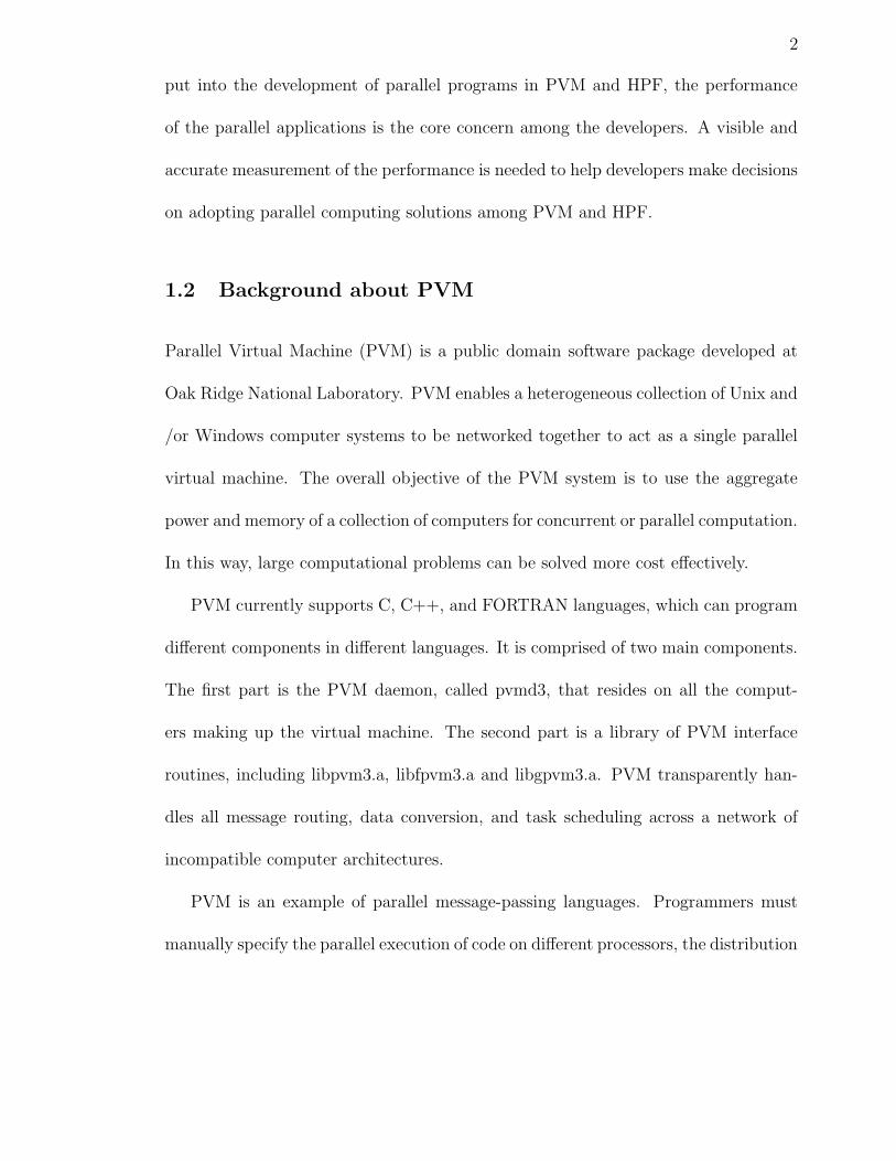
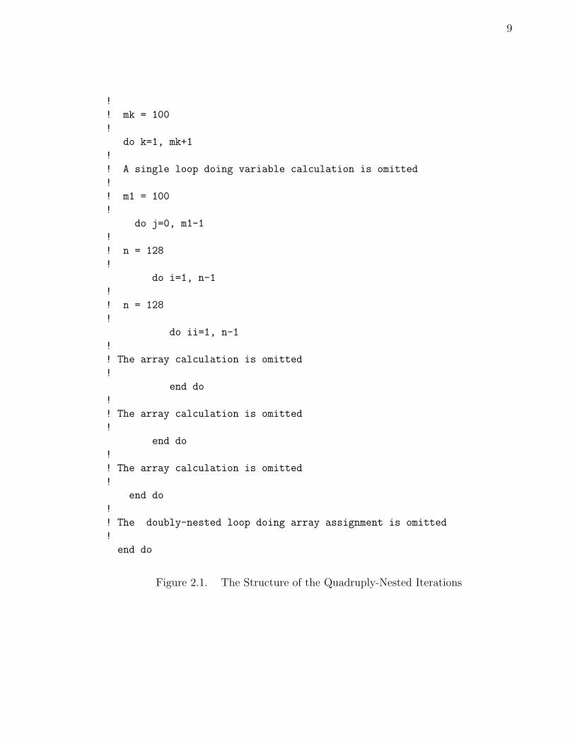
The WRS code was implemented in FORTRAN 90 by Barbara Zubik-Kowal. It does

differentiation matrix calculations. The inner core of the main program was composed

of a quadruply-nested loop, one three-dimensional array and two two-dimensional

arrays. The outer-most loop iterates 100 times, the second-inner loop iterates 100

times, the third-inner loop iterated 128 times and the inner-most loop iterates 128

times. Profiling shows that the third-inner loop takes up about 93.4% of the total

execution time. Figure 2.1 shows the structure of the quadruply-nested iterations.

The sketch code of this nested loops in FORTRAN 90 is shown in Appendix A.1.

Since the scalar variable calculation in the third-inner loop is independent of each

other, this loop is suited for parallel implementation. A simple partitioning scheme

works well for the parallel computation.

9

!

! mk = 100

!

do k=1, mk+1

!

! A single loop doing variable calculation is omitted

!

! m1 = 100

!

do j=0, m1-1

!

! n = 128

!

do i=1, n-1

!

! n = 128

!

do ii=1, n-1

!

! The array calculation is omitted

!

end do

!


!

end do

!


!

end do

!

! The doubly-nested loop doing array assignment is omitted

!

end do

Figure 2.1. The Structure of the Quadruply-Nested Iterations

10

2.2 Ocean Currents Simulation (OCS) Code

The OCS code was implemented by Jodi Mead to simulate the forcing of the ocean,

the noise with the direct representer, and multiple floats. Despite the subroutine

calls to initialize the ocean conditions and plot how floats are changing with time,

which costs constant time, the most computationally intensive part of the code is a

doubly-nested loop in the main program. It uses data from previous iteration to find

the coefficients in the linear model, gets the solution of the linear forward model to

form the priors, calculates the matrix with 120 representers, does the final sweep, and

updates the floats.

There are four subroutine calls inside the inner loop residing in the doubly-nested

loop. The job of these subroutines includes initializing and finding the impulse for the

specific representer, finding the solution from the adjoint model, finding the weights

in the forward representer model , and finally finding the mth representer solution

and putting it in the mth row of the representer matrix.

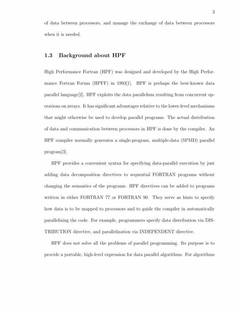
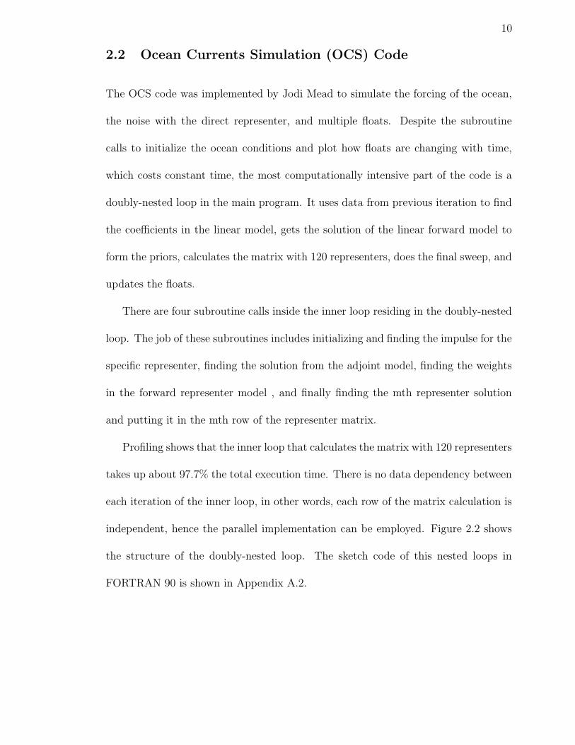
Profiling shows that the inner loop that calculates the matrix with 120 representers

takes up about 97.7% the total execution time. There is no data dependency between

each iteration of the inner loop, in other words, each row of the matrix calculation is

independent, hence the parallel implementation can be employed. Figure 2.2 shows

the structure of the doubly-nested loop. The sketch code of this nested loops in

FORTRAN 90 is shown in Appendix A.2.

11

!

! nn=3

!

do n=1,nn

call coef(...)

call oceLmodel(...)

!

! mm=120

!

do m=1,mm

call impulse(...)

call adjLmodel(...)

call weights(...)

call oceLmodel(...)

!

! Omit forall-statement



!

end do

call impulse(...)

call adjLmodel(...)

call weights(...)

call oceLmodel(...)

call time_plot(...)

end do

Figure 2.2. The Structure of the Doubly-Nested Iterations

12

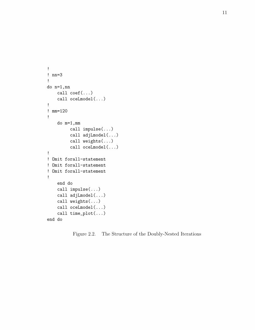
The outer loop also contains some I/O operations and matrix calculations that

take constant time. However, these take an insignificant amount of time and are

hence omitted from the sketch shown above.

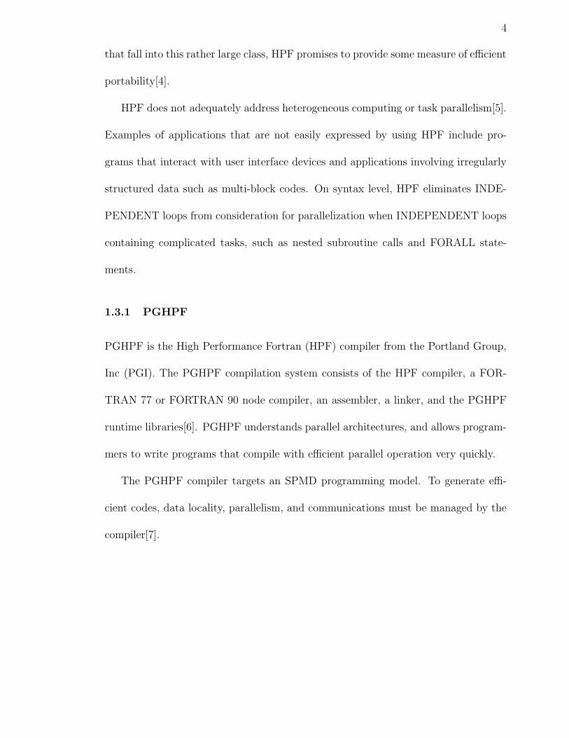
The following Figure 2.3 shows subroutine call relationships in the sequential

program.

lam_allderv2

oceLmodel impulse adjLmodel weights time_plotCoef

time_derv2

th_allderv2

time_allderv2

th_allderv

lam_allderv

time_allderv

time_derv

aderv

bderv

aderv

bderv

Main Program

Figure 2.3. The Flow Chart of Subroutine Calls for OCS Code

13

2.3 Inversion of Controlled Source Audio-Frequency Magne-

totelluric Data (ICSAMD) Code

The ICSAMD code was implemented by Partha Routh to perform inversion of con-

trolled source audio-frequency magnetotelluric data for a horizontally layered earth

model. The major program contains over 8,800 lines of code. There are a total of

42 subroutines and functions. It takes around 12 hours and 30 minutes to run the

program on one processor.

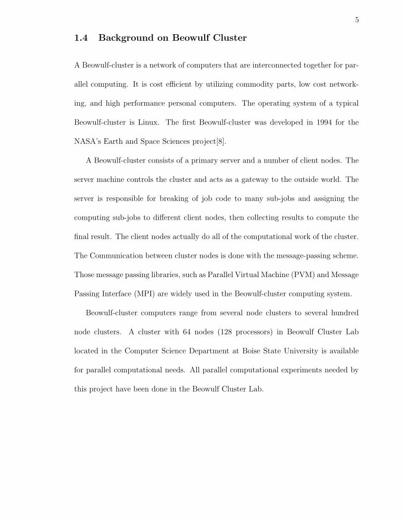
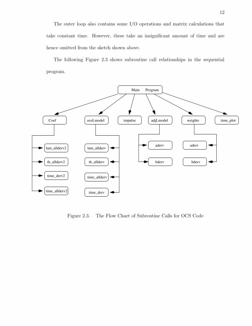
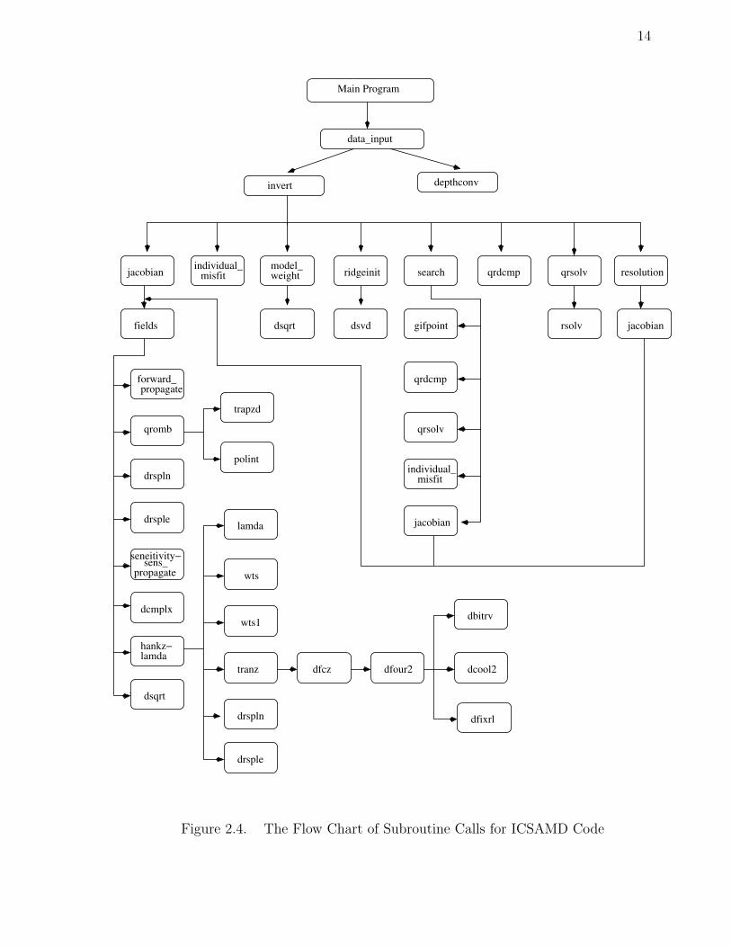
The Figure 2.4 shows the subroutine call relationships in the sequential program.

There are up to eleven layers of subroutine calls.

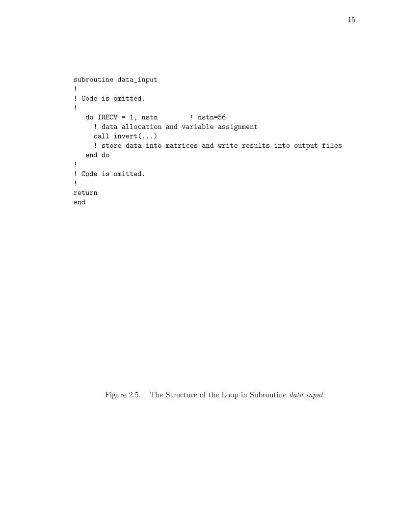
Profiling shows that the loop inside subroutine data input takes up about 97.8%

of the total execution time. This loop iterates 56 times. In each iteration, it calls

subroutine invert to perform intensive computation for inversion and stores results

in the output files. Since there is no data dependency between each loop iteration,

parallel implementation can be employed.

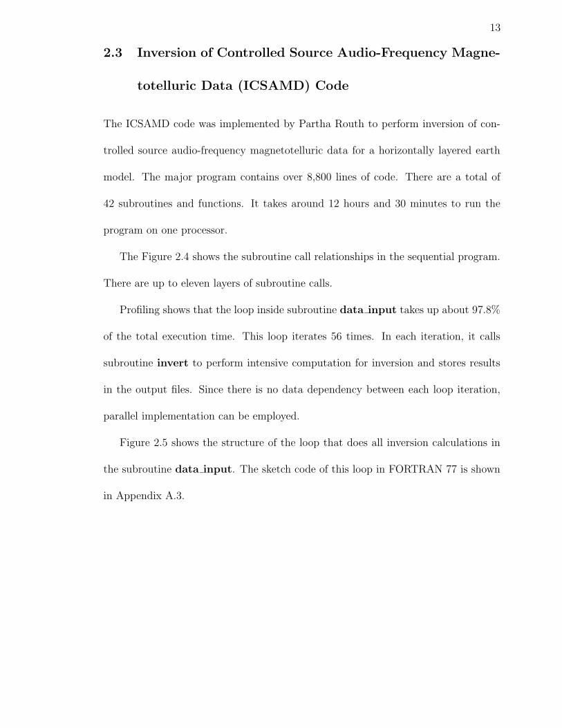
Figure 2.5 shows the structure of the loop that does all inversion calculations in

the subroutine data input. The sketch code of this loop in FORTRAN 77 is shown

in Appendix A.3.

14

Main Program

depthconvinvert

data_input

model_weight ridgeinit search qrsolv resolution

individual_misfit

forward_propagate

seneitivity−

propagate

drspln

qromb

drsple

hankz−lamda

sens_

polint

trapzd

qrdcmp

individual_misfit

jacobian

dbitrv

dcool2

dfixrl

dfour2 dfcz

lamda

wts

wts1

tranz

drspln

drsple

dsqrt

dcmplx

rsolv jacobian

qrdcmp

gifpoint

qrsolv

dsvddsqrtfields

jacobian

Figure 2.4. The Flow Chart of Subroutine Calls for ICSAMD Code

15

subroutine data_input

!

! Code is omitted.

!

do IRECV = 1, nstn ! nstn=56

! data allocation and variable assignment

call invert(...)

! store data into matrices and write results into output files

end do

!

! Code is omitted.

!

return

end

Figure 2.5. The Structure of the Loop in Subroutine data input

Chapter 3

PARALLELIZING APPLICATIONS IN PVM

PVM has excellent support for MPMD (MIMD) and SPMD (SIMD) models of parallel

programming. In the SPMD model, the tasks will execute the same set of instructions

but on different pieces of data. In the MPMD model, each task executes different

instructions on different data. The required PVM control statements need to be

inserted to the source program to select which portions of the code will be executed

by each processor in order to separate the actions of each process.

• The SPMD Computational Model

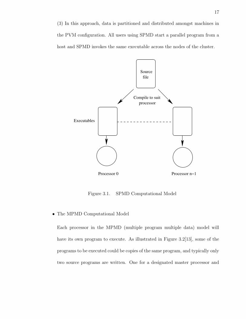
(1) The SPMD (single program multiple data) model is ideal where each process

will actually execute the same source code. The program is compiled into exe-

cutable code for each processor, as illustrated in Figure 3.1[12]. Each processor

will load a copy of this code into its local memory for execution. Usually there

is one controlling process, a “master process”, and the remainder are “slaves”

or “workers”.

(2) Every processor receives the same program. However, each processor may

be assigned to execute a different part of the program by the programmer.

17

(3) In this approach, data is partitioned and distributed amongst machines in

the PVM configuration. All users using SPMD start a parallel program from a

host and SPMD invokes the same executable across the nodes of the cluster.

Executables

Compile to suitprocessor

Processor 0 Processor n−1

Source file

Figure 3.1. SPMD Computational Model

• The MPMD Computational Model

Each processor in the MPMD (multiple program multiple data) model will

have its own program to execute. As illustrated in Figure 3.2[13], some of the

programs to be executed could be copies of the same program, and typically only

two source programs are written. One for a designated master processor and

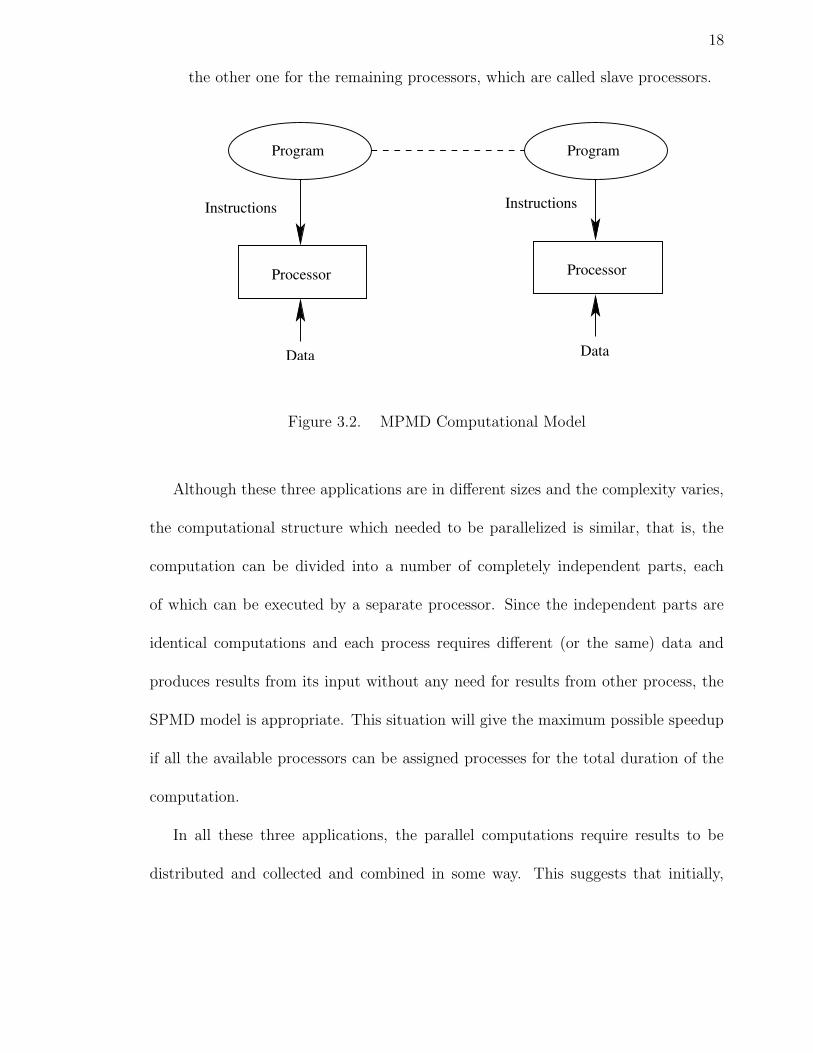
18

the other one for the remaining processors, which are called slave processors.

Instructions Instructions

Data Data

Program

Processor Processor

Program

Figure 3.2. MPMD Computational Model

Although these three applications are in different sizes and the complexity varies,

the computational structure which needed to be parallelized is similar, that is, the

computation can be divided into a number of completely independent parts, each

of which can be executed by a separate processor. Since the independent parts are

identical computations and each process requires different (or the same) data and

produces results from its input without any need for results from other process, the

SPMD model is appropriate. This situation will give the maximum possible speedup

if all the available processors can be assigned processes for the total duration of the

computation.

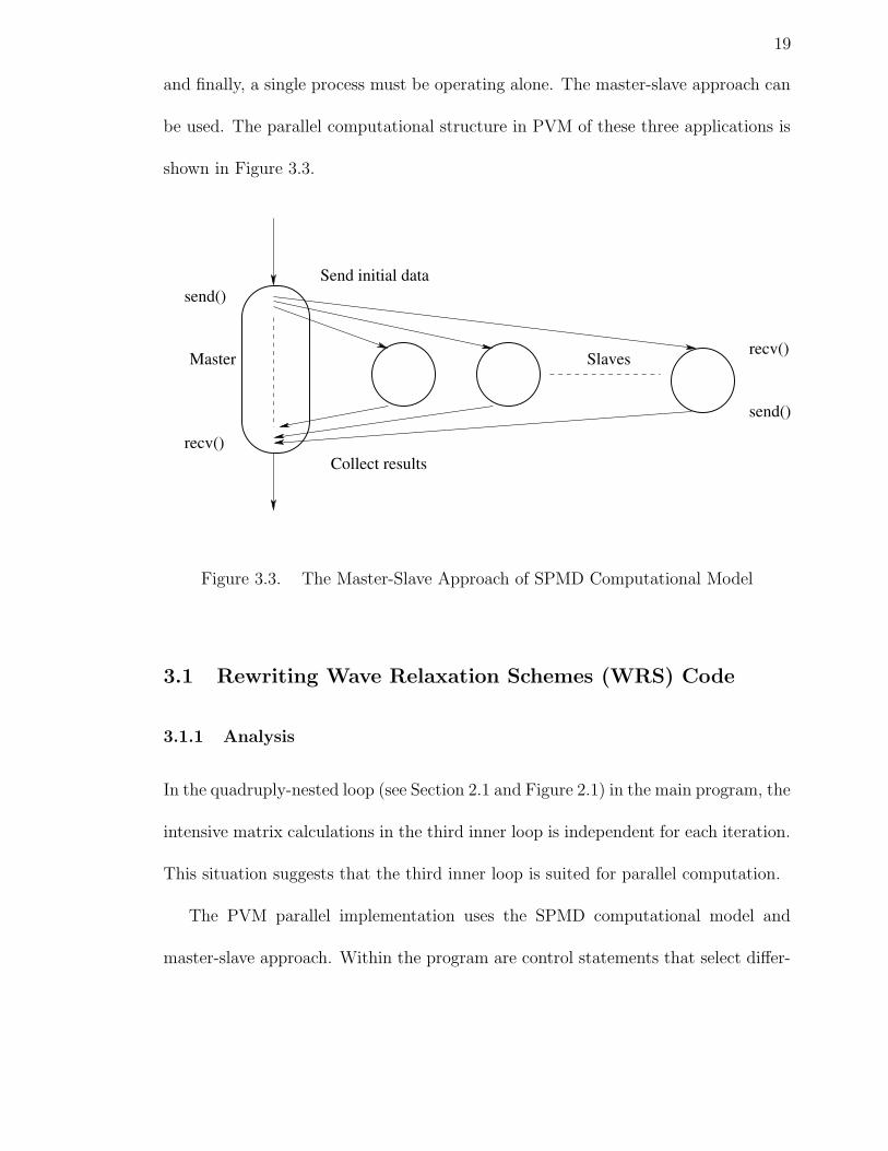
In all these three applications, the parallel computations require results to be

distributed and collected and combined in some way. This suggests that initially,

19

and finally, a single process must be operating alone. The master-slave approach can

be used. The parallel computational structure in PVM of these three applications is

shown in Figure 3.3.

Slavesrecv()

send()

Collect results

Master

send()

recv()

Send initial data

Figure 3.3. The Master-Slave Approach of SPMD Computational Model

3.1 Rewriting Wave Relaxation Schemes (WRS) Code

3.1.1 Analysis

In the quadruply-nested loop (see Section 2.1 and Figure 2.1) in the main program, the

intensive matrix calculations in the third inner loop is independent for each iteration.

This situation suggests that the third inner loop is suited for parallel computation.

The PVM parallel implementation uses the SPMD computational model and

master-slave approach. Within the program are control statements that select differ-

20

ent parts of code for each process. The user can start the parallel program from a

host and SPMD distributes the same executable to other processes. After the master

process has been determined, all the other processes will work as slaves. The simple

partitioning scheme for task assignment is appropriate.

First, each slave process needs to find its part of the job in the parallel computation

in the third inner loop, which is, the computation of a portion of one column in the

matrix. The computation of one column of the matrix is simply divided into separate

parts and each part is computed separately by each slave process.

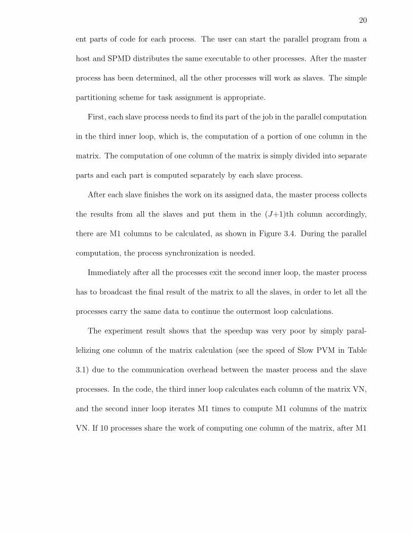
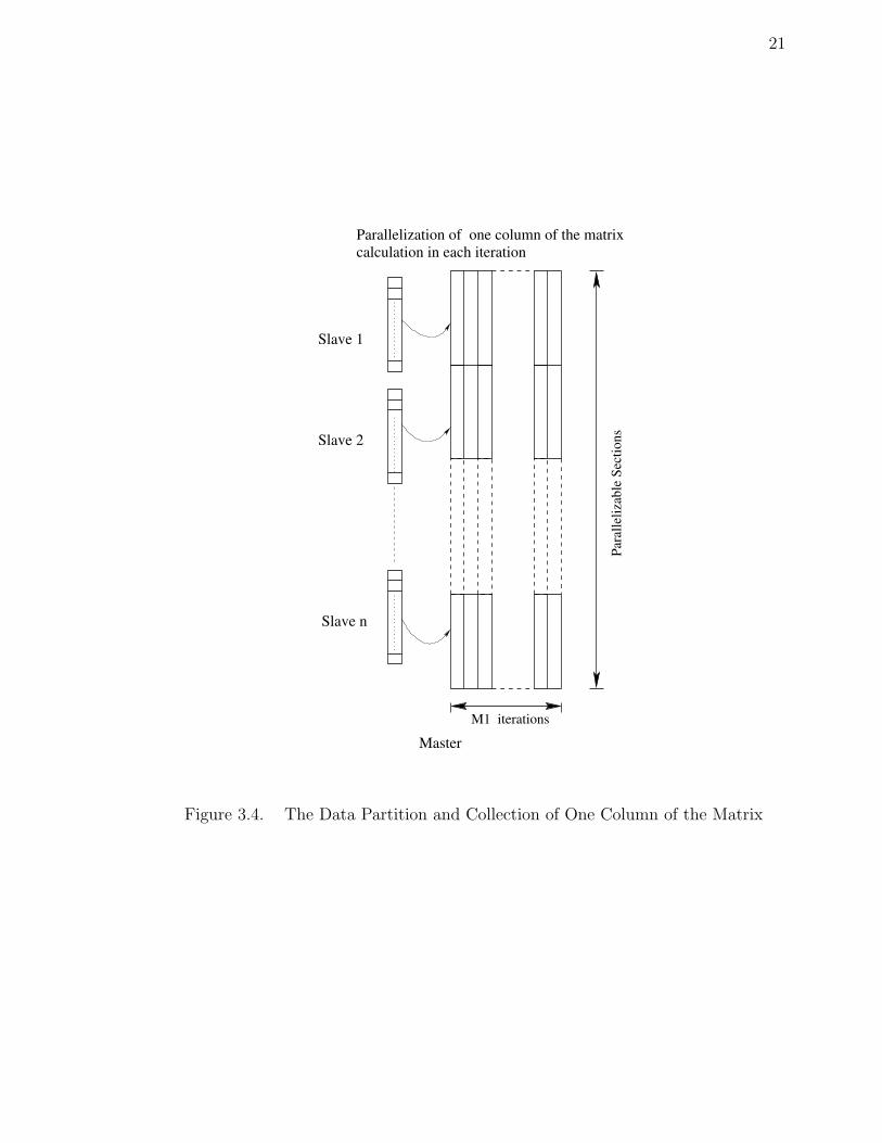
After each slave finishes the work on its assigned data, the master process collects

the results from all the slaves and put them in the (J+1)th column accordingly,

there are M1 columns to be calculated, as shown in Figure 3.4. During the parallel

computation, the process synchronization is needed.

Immediately after all the processes exit the second inner loop, the master process

has to broadcast the final result of the matrix to all the slaves, in order to let all the

processes carry the same data to continue the outermost loop calculations.

The experiment result shows that the speedup was very poor by simply paral-

lelizing one column of the matrix calculation (see the speed of Slow PVM in Table

3.1) due to the communication overhead between the master process and the slave

processes. In the code, the third inner loop calculates each column of the matrix VN,

and the second inner loop iterates M1 times to compute M1 columns of the matrix

VN. If 10 processes share the work of computing one column of the matrix, after M1

21

Slave 1

Slave 2

Slave n

Master

Parallelization of one column of the matrixcalculation in each iteration

Para

lleliz

able

Sec

tions

M1 iterations

Figure 3.4. The Data Partition and Collection of One Column of the Matrix

22

iterations of the second inner loop, there will be at least 10*M1 messages passing

between slaves and the master.

TABLE 3.1: Speed Comparison between the Slow PVM Version and the Fast PVMVersion

Parameters Process NumberN M 1 5 10 15 20 25 30128 100 Slow PVM(secs) 2.11 3.91 5.78 8.26 10.91 14.17 19.47

Fast PVM(secs) 2.10 1.20 1.56 1.95 2.79 3.22 4.07

It was found that the computation of each entry of the matrix depends on the

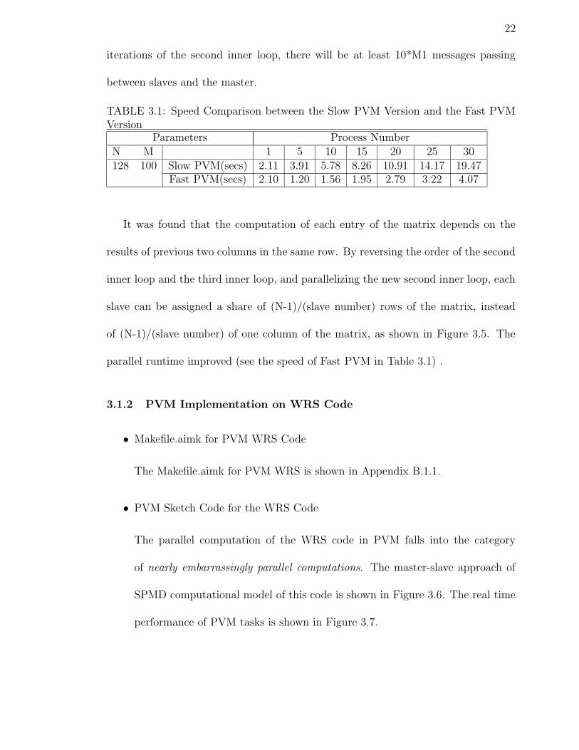
results of previous two columns in the same row. By reversing the order of the second

inner loop and the third inner loop, and parallelizing the new second inner loop, each

slave can be assigned a share of (N-1)/(slave number) rows of the matrix, instead

of (N-1)/(slave number) of one column of the matrix, as shown in Figure 3.5. The

parallel runtime improved (see the speed of Fast PVM in Table 3.1) .

3.1.2 PVM Implementation on WRS Code

• Makefile.aimk for PVM WRS Code

The Makefile.aimk for PVM WRS is shown in Appendix B.1.1.

• PVM Sketch Code for the WRS Code

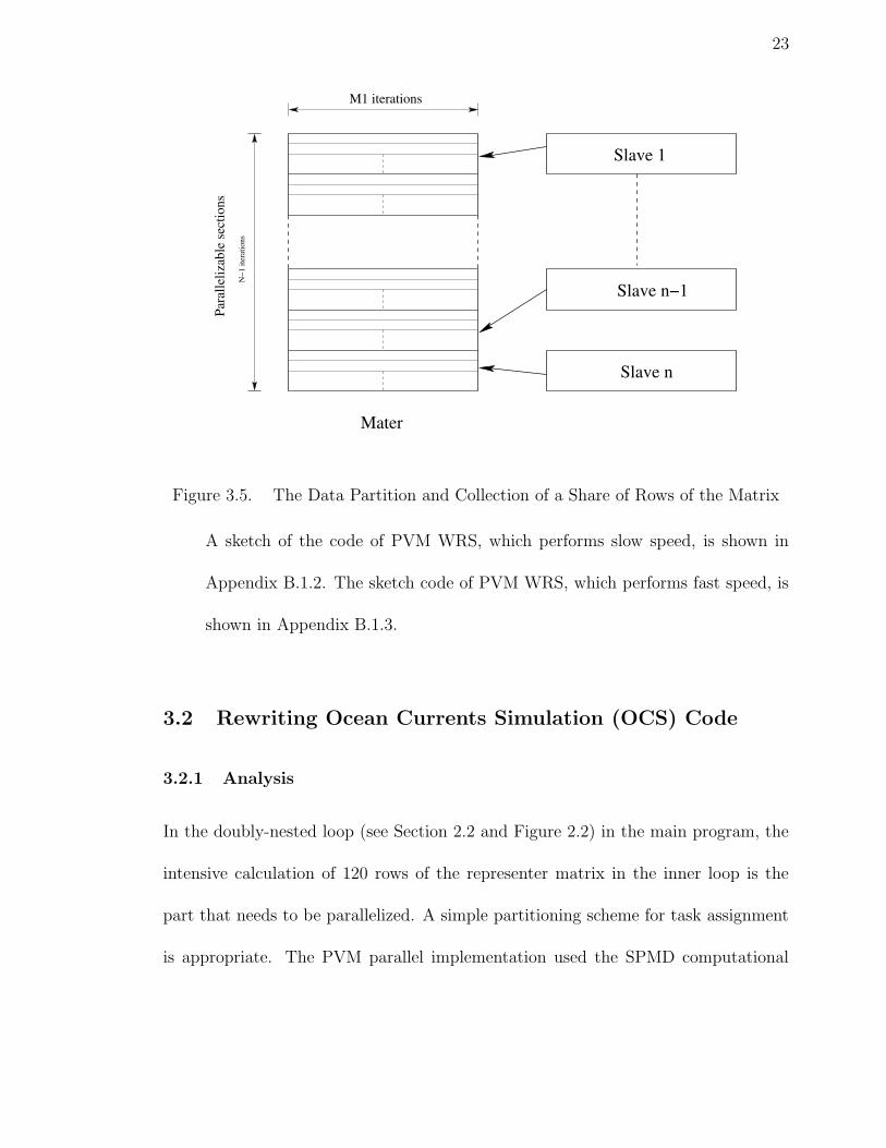
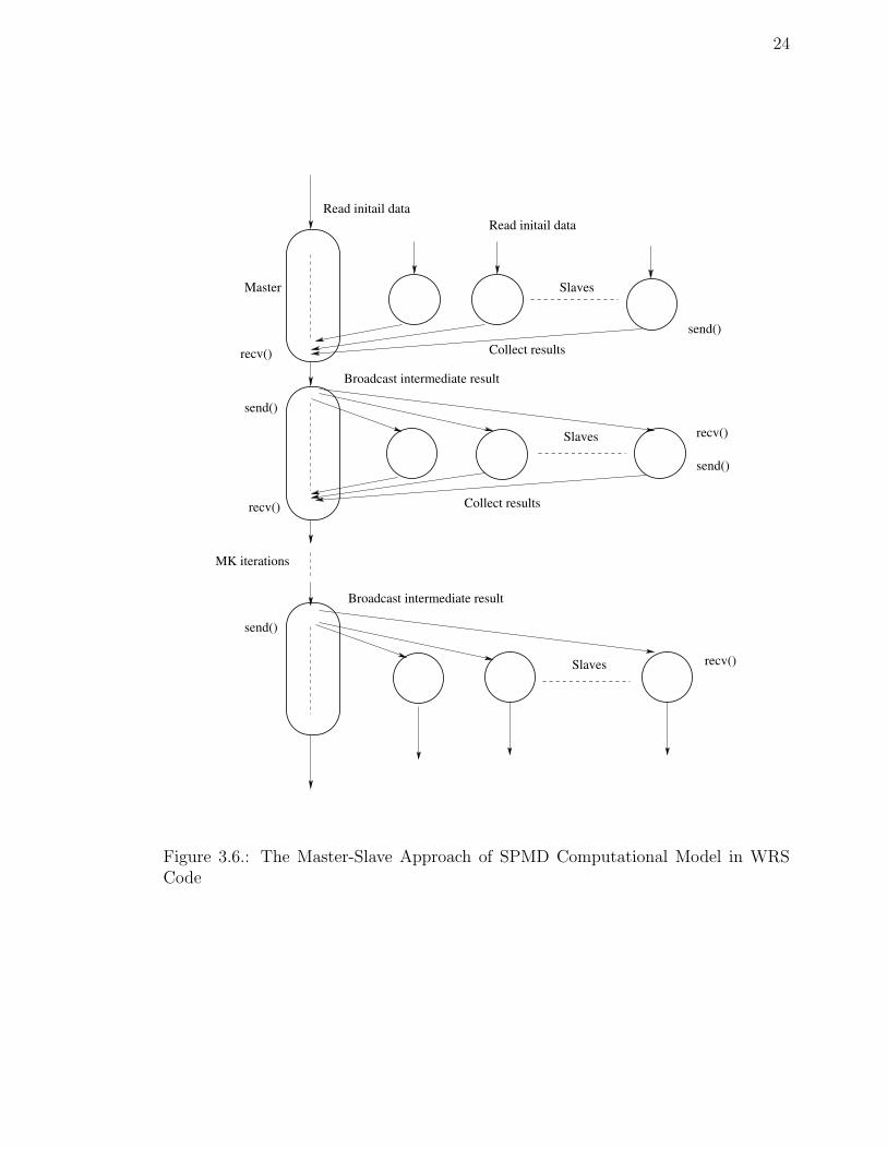
The parallel computation of the WRS code in PVM falls into the category

of nearly embarrassingly parallel computations. The master-slave approach of

SPMD computational model of this code is shown in Figure 3.6. The real time

performance of PVM tasks is shown in Figure 3.7.

23

Mater

Slave 1

Slave n−1

Slave n

M1 iterations

Para

lleliz

able

sec

tions

N−1

iter

atio

ns

Figure 3.5. The Data Partition and Collection of a Share of Rows of the Matrix

A sketch of the code of PVM WRS, which performs slow speed, is shown in

Appendix B.1.2. The sketch code of PVM WRS, which performs fast speed, is

shown in Appendix B.1.3.

3.2 Rewriting Ocean Currents Simulation (OCS) Code

3.2.1 Analysis

In the doubly-nested loop (see Section 2.2 and Figure 2.2) in the main program, the

intensive calculation of 120 rows of the representer matrix in the inner loop is the

part that needs to be parallelized. A simple partitioning scheme for task assignment

is appropriate. The PVM parallel implementation used the SPMD computational

24

Slaves

send()

Master

recv() Collect results

recv()

send()

Slaves

send()

recv()

Collect results

Read initail dataRead initail data

send()

recv()Slaves

Broadcast intermediate result

Broadcast intermediate result

MK iterations

Figure 3.6.: The Master-Slave Approach of SPMD Computational Model in WRSCode

25

Figure 3.7. The Real Time Performance Snapshot of PVM WRS

26

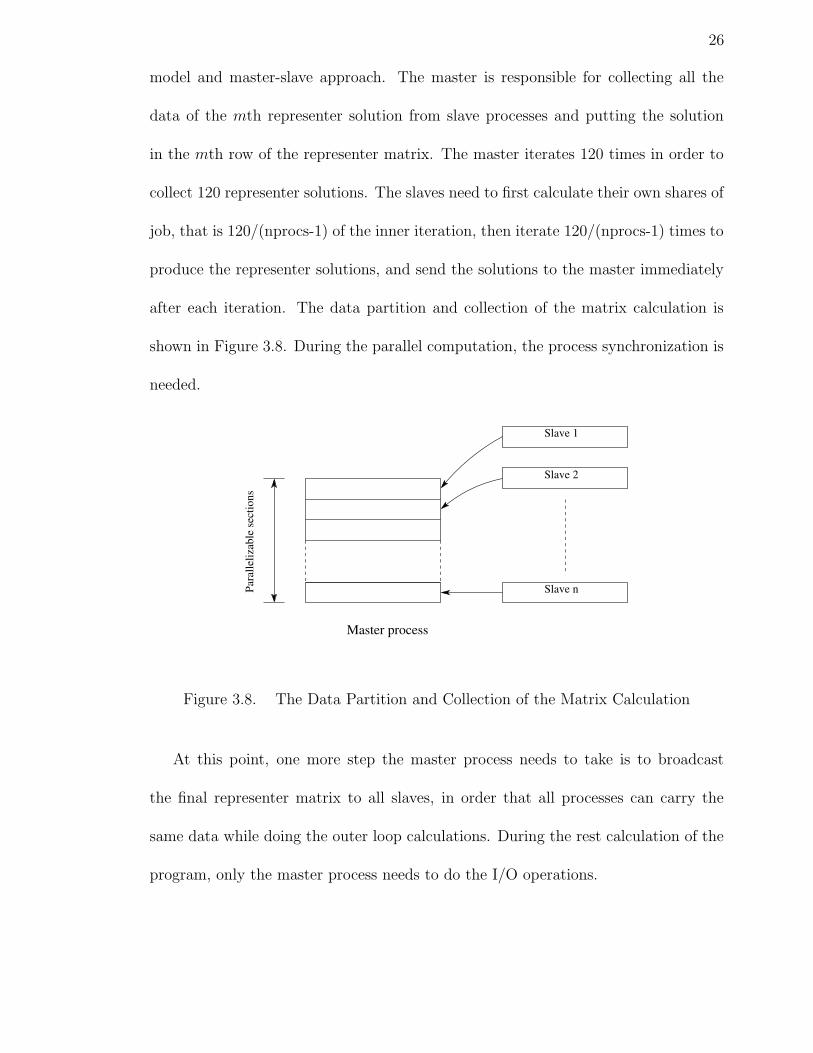
model and master-slave approach. The master is responsible for collecting all the

data of the mth representer solution from slave processes and putting the solution

in the mth row of the representer matrix. The master iterates 120 times in order to

collect 120 representer solutions. The slaves need to first calculate their own shares of

job, that is 120/(nprocs-1) of the inner iteration, then iterate 120/(nprocs-1) times to

produce the representer solutions, and send the solutions to the master immediately

after each iteration. The data partition and collection of the matrix calculation is

shown in Figure 3.8. During the parallel computation, the process synchronization is

needed.

Master process

Slave n

Slave 2

Slave 1

Para

lleliz

able

sec

tions

Figure 3.8. The Data Partition and Collection of the Matrix Calculation

At this point, one more step the master process needs to take is to broadcast

the final representer matrix to all slaves, in order that all processes can carry the

same data while doing the outer loop calculations. During the rest calculation of the

program, only the master process needs to do the I/O operations.

27

3.2.2 PVM Implementation on OCS Code

• Makefile.aimk for PVM OCS Code

The Makefile.aimk for PVM OCS is shown in Appendix B.2.1.

• PVM Sketch Code for the OCS Code

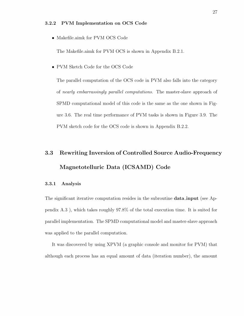
The parallel computation of the OCS code in PVM also falls into the category

of nearly embarrassingly parallel computations. The master-slave approach of

SPMD computational model of this code is the same as the one shown in Fig-

ure 3.6. The real time performance of PVM tasks is shown in Figure 3.9. The

PVM sketch code for the OCS code is shown in Appendix B.2.2.

3.3 Rewriting Inversion of Controlled Source Audio-Frequency

Magnetotelluric Data (ICSAMD) Code

3.3.1 Analysis

The significant iterative computation resides in the subroutine data input (see Ap-

pendix A.3 ), which takes roughly 97.8% of the total execution time. It is suited for

parallel implementation. The SPMD computational model and master-slave approach

was applied to the parallel computation.

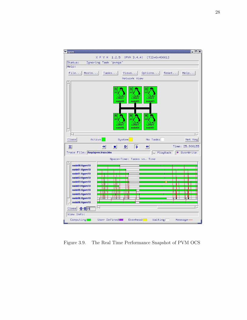
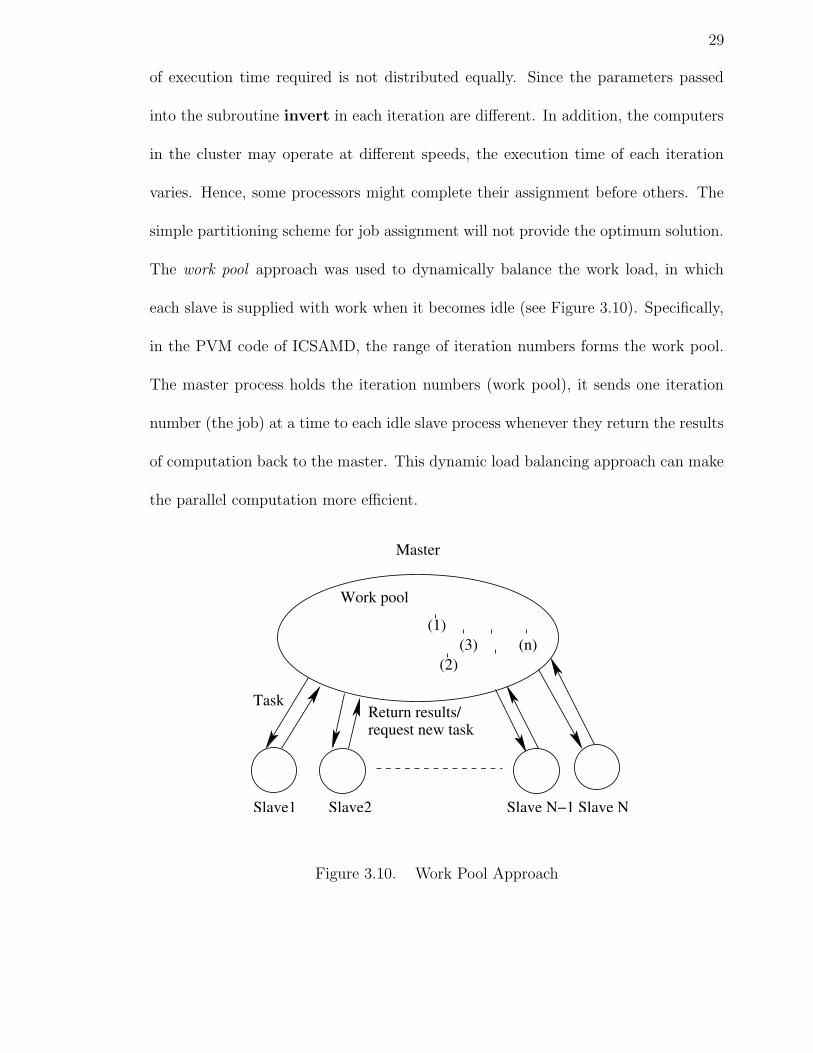
It was discovered by using XPVM (a graphic console and monitor for PVM) that

although each process has an equal amount of data (iteration number), the amount

28

Figure 3.9. The Real Time Performance Snapshot of PVM OCS

29

of execution time required is not distributed equally. Since the parameters passed

into the subroutine invert in each iteration are different. In addition, the computers

in the cluster may operate at different speeds, the execution time of each iteration

varies. Hence, some processors might complete their assignment before others. The

simple partitioning scheme for job assignment will not provide the optimum solution.

The work pool approach was used to dynamically balance the work load, in which

each slave is supplied with work when it becomes idle (see Figure 3.10). Specifically,

in the PVM code of ICSAMD, the range of iteration numbers forms the work pool.

The master process holds the iteration numbers (work pool), it sends one iteration

number (the job) at a time to each idle slave process whenever they return the results

of computation back to the master. This dynamic load balancing approach can make

the parallel computation more efficient.

Slave1 Slave2 Slave N−1 Slave N

Master

TaskReturn results/request new task

Work pool

(1)

(2)(3) (n)

Figure 3.10. Work Pool Approach

30

3.3.2 PVM Implementation on ICSAMD Code

• Makefile.aimk for PVM ICSAMD Code

The sequential ICSAMD code was originally written in FORTRAN 77 and

compiled on Absoft Compiler. The output was not consistent with the re-

sults obtained by using the Portland Group Compiler Technology FORTRAN

77 compiler– pgf77. In order to achieve the consistent results and very close

speed as those produced by the Absoft Compiler, the original Makefile has been

modified by adding the options such as -fast -Kieee -pc 64. The Makefile.aimk

for PVM ICSAMD is based on the modified Makefile. It is shown in Appendix

B.3.1.

• PVM Sketch Code for the ICSAMD Code

The parallel routines need to be started in the main program (see Appendix

B.3.2). All processes call the subroutine data input. The subroutine data input

carries the parallel parameters, such as the process number, the array of the

task identifiers, the task identifier of the calling PVM process, and the number

of task identifiers that were spawned together. The parallel computations run

in the subroutine data input(also see Appendix B.3.2).

In the subroutine data input, the main job for the master process is doing the

I/O operation and handling the work pool, and for the slaves it is to carry

the computation of inversion. The parallel computation in the subroutine

31

data input is as following: the master process opens input files and reads

the data, then sends them to the slave processes. After the slaves receive the

data from the master, all processes need to allocate the memory for the global

variables.

Next, the master allocates the memory for the local variables, then keeps on

sending tasks from the work pool to the slaves, receiving data from all the slaves

and writing them into the output files. Finally the master closes the output files

and frees the memory of the local variables.

In the meantime, each slave is first given one iteration number by the master to

do the inversion computation. From then on, the slave gets another one when

it returns a result, until there are no more numbers in the work pool. So, the

slaves either get a new task or get a termination message to terminate their work

when they ask master to give them a new task. After receiving a new job, the

slaves need to allocate memory for the local variables and call the subroutine

invert to start a computation of inversion. When they finish the computation

of inversion, they need to send the output data returned from the subroutine

invert to the master process, and free the memory of local variables.

At the end, all processes free the memory of the global variables. During the

whole parallelizing computation, process synchronization is needed. The PVM

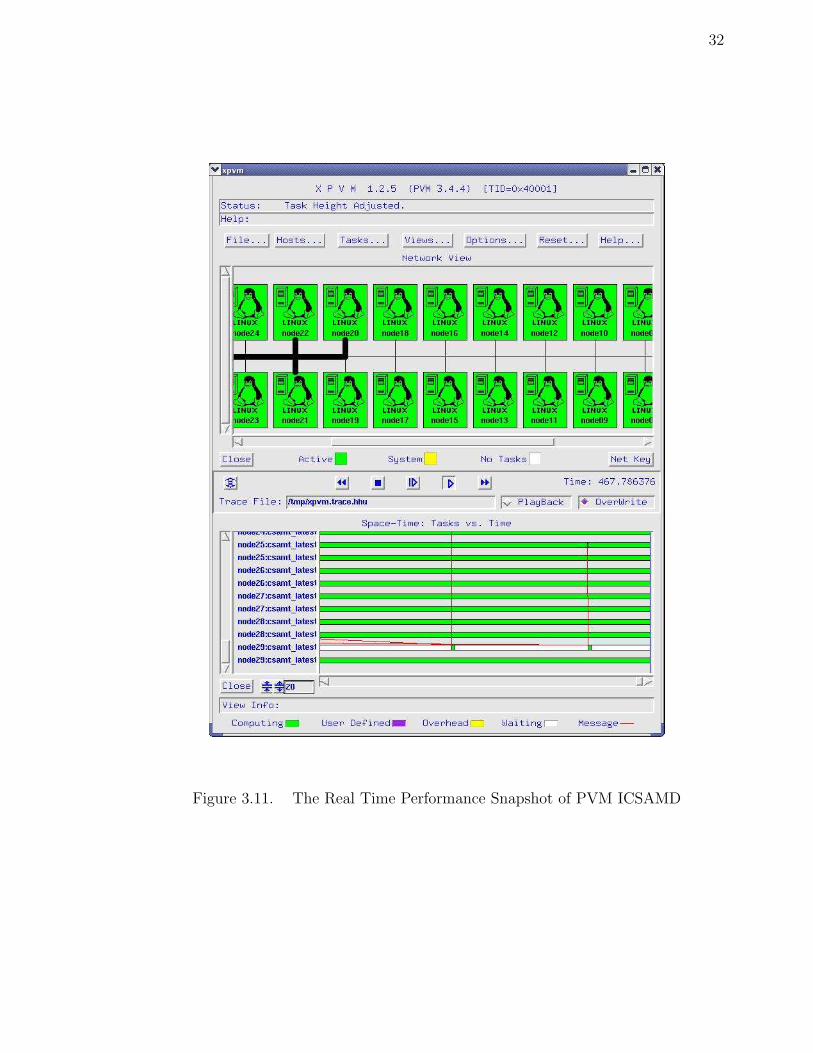
sketch code for the ICSAMD is shown in Appendix B.3.2. The real time per-

formance of PVM tasks is shown in Figure 3.11.

32

Figure 3.11. The Real Time Performance Snapshot of PVM ICSAMD

Chapter 4

PARALLELIZING APPLICATIONS IN HPF

In order to simulate the parallel implementation process that people with no knowl-

edge of HPF are required to go through, a reasonable learning curve has been put into

the experiment. The author spent one week studying the basic knowledge of HPF

before starting to convert FORTRAN code into HPF code. The learning process was

accompanied with the whole period of the HPF implementation on three programs,

which lasted six weeks.

4.1 Rewriting Wave Relaxation Schemes (WRS) Code

4.1.1 Analysis

In the nested loop (see Section 2.1 and Figure 2.1), the scalar variable calculation for

the two-dimensional array inside the third-inner loop may be executed independently—

that is, in any order, or interleaved, or concurrently—without changing the semantics

of the program. The directive INDEPENDENT preceding the third-inner DO loop

may enable the parallel execution. The mechanism underneath is that the INDE-

PENDENT directive asserts to the compiler that all the iterations in this DO loop

34

can be operated independently. Each node or processor on the parallel system will

execute its part of computation of DO loop.

There are two compiler-replicated variables inside the loop preventing the paral-

lelization. They need to be treated as private variables inside the body of DO loop

instead of causing error. In order to make these variables to be undefined immediately

before and after each iteration of the loop, they have to be put into the variable-list in

a NEW clause. The index variable for the DO loop must also be declared NEW[14].

There is one scalar accumulator appearing in four reduction statements inside

the DO loop. Since the accumulator is compiler-replicated, it needs to be put into

REDUCTION clause acknowledging the compiler to perform reductions locally on

all processors. Since all four reduction statements work for one accumulator, they

can be combined into one statement to reduce the work of the compiler. The code

modification is needed.

After the NEW clause and the REDUCTION clause have been added to INDE-

PENDENT directive to assist parallelization of the INDEPENDENT loop, one more

step has to be taken into account, that is the data distribution. In order to obtain

the highest speed, the two-dimensional array inside the parallelized DO loop has to

be distributed among the memory of processors. The DISTRIBUTE directive will

work. Since PGHPF strictly obeys the INDEPENDENT annotations, it redistributes

arrays before and after loop nests so that all the annotation specified parallelism is

exploited.

35

4.1.2 The HPF implementation on WRS Code

(1) Add PGHPF compiler options to Makefile

Most FORTRAN node compiler options are also valid for PGHPF. In this case, be-

sides the original FORTRAN compiler option, PGHPF Option -Mautopar and -Mmpi

have been added to the Makefile to enable the auto-parallelization of FORTRAN DO

loop in MPI environment. The example of the Makefile for WRS is in Appendix

C.1.1.

(2) Comparison of the Sketch Codes in FORTRAN and in HPF

The sketch code of WRS in FORTRAN 90 is in Appendix A.1. The sketch code

of WRS in HPF is in Appendix C.1.2.

4.2 Rewriting Ocean Currents Simulation (OCS) Code

4.2.1 Analysis

Based on the successful experience obtained from implementing HPF version of WRS

program, the first step to parallelize the inner loop (see Section 2.2 and Figure 2.2)

that iterates 120 times to calculate 120 rows of the representer matrix independently

is to insert INDEPENDENT directive proceeding the loop. The difference is that

this independent loop contains subroutine calls instead of array calculations.

A PURE prefix needs to be added to those subroutines called in the INDEPEN-

DENT loop to assert to the compiler that no communication will be generated be-

tween these subroutines. Any subroutine referenced in a pure subroutine is also

36

declared pure. An INTERFACE for each of these pure subroutines has to be declared

explicitly. The PURE attribute needs to be specified inside the INTERFACE block.

There are three FORALL assignments inside the inner loop. Although FORALL

assignments can carry-out tightly-coupled parallel executions, they may cause the

compiler’s confusion inside INDEPENDENT DO loop, hence will prevent paralleliza-

tion of the INDEPENDENT loops. The modification of FORALL assignments into

regular DO loops has been made.

After adding HPF directives, the template for the independent loop’s home array

has been created by the compiler, but the independent loop has not been successfully

parallelized due to the dependency conflicts or possible misalignment of a set of

dummy variables in the subroutine-calls inside the loop. The program has to be

restructured by creating a different set of dummy variables, and copying the values

of original dummy variables into them just before the INDEPENDENT loop. The

array initializations before each subroutine calls have been moved into corresponding

subroutines.

After all the above efforts, the INDEPENDENT loop is now parallelized success-

fully, and the performance of the program has been improved significantly.

4.2.2 The HPF implementation on OCS Code


PGHPF Option -Mautopar and -Mmpi are added to the Makefile to enable the

auto-parallelization of FORTRAN DO loop in MPI environment. Appendix C.2.1

37

shows the example of the Makefile.

(2) Comparison of the sketch code between FORTRAN OCS and HPF OCS

The sketch code of OCS in FORTRAN 90 is in Appendix A.2. The sketch code

of OCS in HPF is in Appendix C.2.2.

4.3 Rewriting Inversion of Controlled Source Audio-Frequency

Magnetotelluric Data (ICSAMD) Code

4.3.1 Analysis

(1) Converting Sequential code into HPF

Since there is no data dependency between each iteration doing inversion, the

INDEPENDENT loop can be applied to the loop inside data input subroutine.

Therefore, the INDEPENDENT directive is inserted proceeding the loop. The PURE

prefixes are added to those functions and subroutine statements which are called in-

side the loop. In addition, an INTERFACE for each of these pure functions and

subroutines is declared explicitly with the PURE attributes specified inside the IN-

TERFACE block. Those compiler-replicated variable names appearing in the loop are

listed in the NEW clause to assist the compiler in parallelizing the INDEPENDENT

loop.

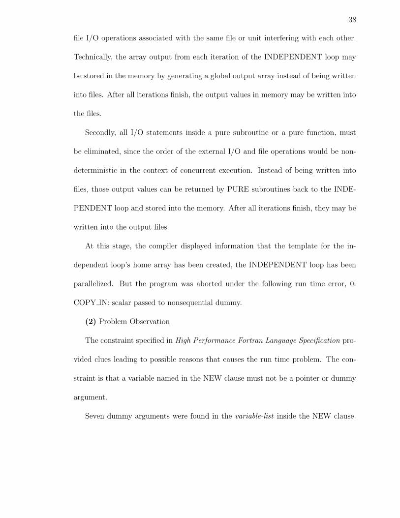
Here are some constraints that need to be taken into consideration to prevent side

effects before the program is to be compiled. First, the file I/O operations inside

the INDEPENDENT loop need to be moved out of the loop to prevent any two

38

file I/O operations associated with the same file or unit interfering with each other.

Technically, the array output from each iteration of the INDEPENDENT loop may

be stored in the memory by generating a global output array instead of being written

into files. After all iterations finish, the output values in memory may be written into

the files.

Secondly, all I/O statements inside a pure subroutine or a pure function, must

be eliminated, since the order of the external I/O and file operations would be non-

deterministic in the context of concurrent execution. Instead of being written into

files, those output values can be returned by PURE subroutines back to the INDE-

PENDENT loop and stored into the memory. After all iterations finish, they may be

written into the output files.

At this stage, the compiler displayed information that the template for the in-

dependent loop’s home array has been created, the INDEPENDENT loop has been

parallelized. But the program was aborted under the following run time error, 0:

COPY IN: scalar passed to nonsequential dummy.

(2) Problem Observation

The constraint specified in High Performance Fortran Language Specification pro-

vided clues leading to possible reasons that causes the run time problem. The con-

straint is that a variable named in the NEW clause must not be a pointer or dummy

argument.

Seven dummy arguments were found in the variable-list inside the NEW clause.

39

Two ways have been tried to solve the problem. The first attempt was to use -

Minline on the compilation command line to inline procedure calls within the INDE-

PENDENT DO loop. Unfortunately, the program met an internal compiler error:

mk assign sptr: upper bound missing. The second attempt was to restructure the

program by creating a different set of dummy variables, and copying the values of

original dummy variables into them just before the INDEPENDENT loop. It was

a success to convert OCS code into HPF, but failed in the ICSAMD program. The

possible reason for the failure was that the original code writer used pointers and

dynamic allocations inside the INDEPENDENT DO loop which might prevent loop

parallelization.

(3) Another Way to Approach Speedup

By adding -Msequence on the compilation command line, all variables are created

as SEQUENCE variables, where sequential storage is assumed. In the meantime, the

SEQUENCE directives were added to all pure subroutine scope units to explicitly

declare that both variables and common blocks are to be treated by the compiler

as sequential. The compiler message did not display that the INDEPENDENT loop

being parallelized; however, the runtime has been improved by 69%.

4.3.2 The HPF implementation on ICSAMD Code


Just as in the Makefiles for HPF codes of WRS and OCS, PGHPF option -

Mautopar and -Mmpi are added to the Makefile to enable the auto-parallelization

40

of FORTRAN DO loop in the MPI environment. Additionally, PGHPF option -

Msequence was added to create all variables as SEQUENCE variables. Appendix

C.3.1 shows the example of the Makefile.

(2) Comparison of the sketch code between FORTRAN ICSAMD and HPF IC-

SAMD

The sketch code for FORTRAN ICSAMD is shown in Appendix A.3, and the

sketch code for HPF ICSAMD is shown in Appendix C.3.2.

Chapter 5

COMPARISON OF RUNNING SPEED BETWEEN THE

PARALLEL IMPLEMENTATIONS IN PVM VERSUS IN

HPF

A Beowulf-cluster was used for demonstrating the differences of the speedup between

PVM implementations and HPF implementations of WRS code, OCS code and IC-

SAMD code. The cluster has 122 2.4 GHz Intel Xeon processors, 64GB of memory,

2.4 TB of disk space, private Gigabit network and a Gigabit connection to the campus

backbone.

The PCs are running RedHat Linux 9.0 with a version 2.4.24-i686 SMP kernel.

The PGI version 5.0 Cluster Development Kit X86 compilers, in particular, PGF77,

PGF90, PGHPF compilers were applied to the experimentations. PVM version 3.4.4

and XPVM version 1.2.5 [16] are being used.

5.1 The Experiment Result for the WRS Code

Table 5.1 shows the speed of PVM WRS implementation and the speed of HPF WRS

implementation. Both codes are based on the modified sequential code in which the

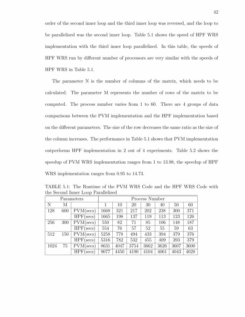
42

order of the second inner loop and the third inner loop was reversed, and the loop to

be parallelized was the second inner loop. Table 5.1 shows the speed of HPF WRS

implementation with the third inner loop parallelized. In this table, the speeds of

HPF WRS run by different number of processors are very similar with the speeds of

HPF WRS in Table 5.1.

The parameter N is the number of columns of the matrix, which needs to be

calculated. The parameter M represents the number of rows of the matrix to be

computed. The process number varies from 1 to 60. There are 4 groups of data

comparisons between the PVM implementation and the HPF implementation based

on the different parameters. The size of the row decreases the same ratio as the size of

the column increases. The performance in Table 5.1 shows that PVM implementation

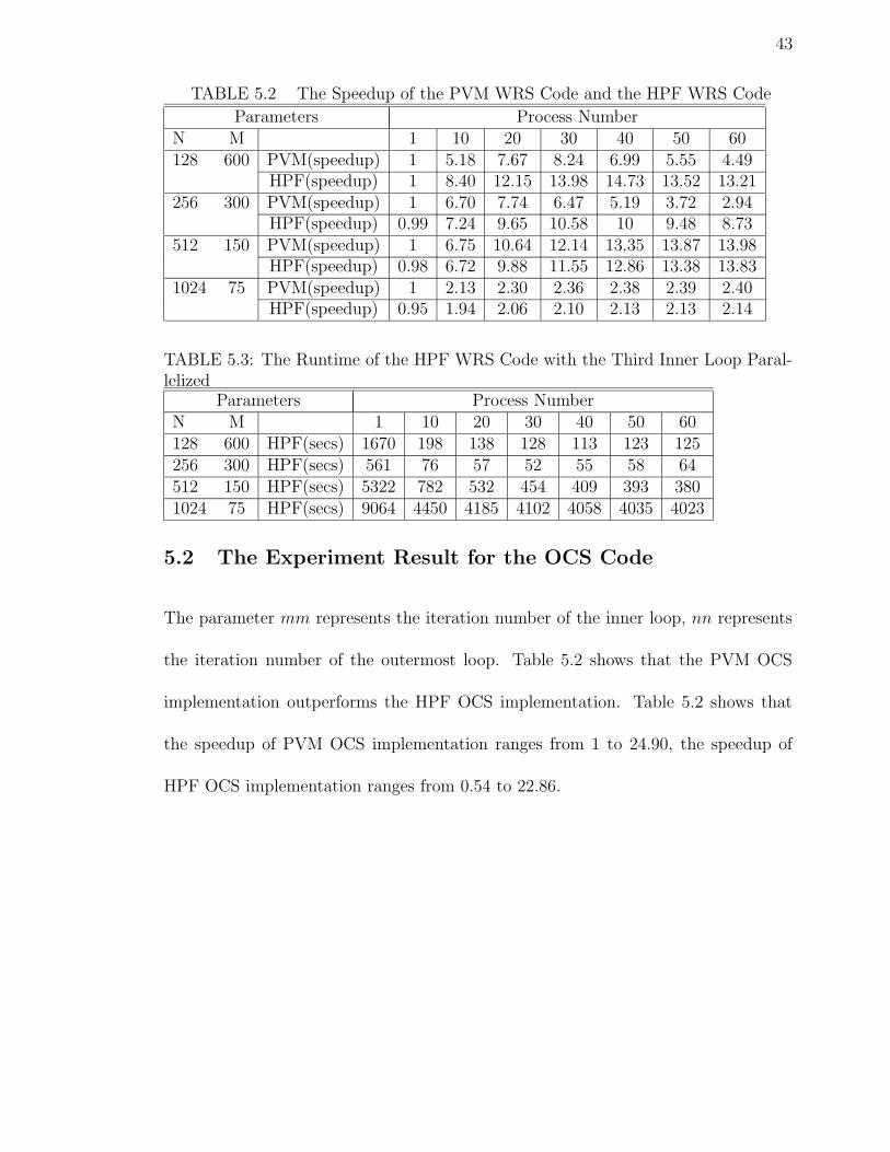
outperforms HPF implementation in 2 out of 4 experiments. Table 5.2 shows the

speedup of PVM WRS implementation ranges from 1 to 13.98, the speedup of HPF

WRS implementation ranges from 0.95 to 14.73.

TABLE 5.1: The Runtime of the PVM WRS Code and the HPF WRS Code withthe Second Inner Loop Parallelized

Parameters Process NumberN M 1 10 20 30 40 50 60128 600 PVM(secs) 1668 321 217 202 238 300 371

HPF(secs) 1665 198 137 119 113 123 126256 300 PVM(secs) 550 82 71 85 106 148 187

HPF(secs) 554 76 57 52 55 59 63512 150 PVM(secs) 5258 778 494 433 394 379 376

HPF(secs) 5316 782 532 455 409 393 3791024 75 PVM(secs) 8631 4047 3754 3662 3626 3607 3600

HPF(secs) 9077 4450 4190 4104 4061 4043 4028

43

TABLE 5.2 The Speedup of the PVM WRS Code and the HPF WRS Code

Parameters Process NumberN M 1 10 20 30 40 50 60128 600 PVM(speedup) 1 5.18 7.67 8.24 6.99 5.55 4.49

HPF(speedup) 1 8.40 12.15 13.98 14.73 13.52 13.21256 300 PVM(speedup) 1 6.70 7.74 6.47 5.19 3.72 2.94

HPF(speedup) 0.99 7.24 9.65 10.58 10 9.48 8.73512 150 PVM(speedup) 1 6.75 10.64 12.14 13.35 13.87 13.98

HPF(speedup) 0.98 6.72 9.88 11.55 12.86 13.38 13.831024 75 PVM(speedup) 1 2.13 2.30 2.36 2.38 2.39 2.40

HPF(speedup) 0.95 1.94 2.06 2.10 2.13 2.13 2.14

TABLE 5.3: The Runtime of the HPF WRS Code with the Third Inner Loop Paral-lelized

Parameters Process NumberN M 1 10 20 30 40 50 60128 600 HPF(secs) 1670 198 138 128 113 123 125256 300 HPF(secs) 561 76 57 52 55 58 64512 150 HPF(secs) 5322 782 532 454 409 393 3801024 75 HPF(secs) 9064 4450 4185 4102 4058 4035 4023

5.2 The Experiment Result for the OCS Code

The parameter mm represents the iteration number of the inner loop, nn represents

the iteration number of the outermost loop. Table 5.2 shows that the PVM OCS

implementation outperforms the HPF OCS implementation. Table 5.2 shows that

the speedup of PVM OCS implementation ranges from 1 to 24.90, the speedup of

HPF OCS implementation ranges from 0.54 to 22.86.

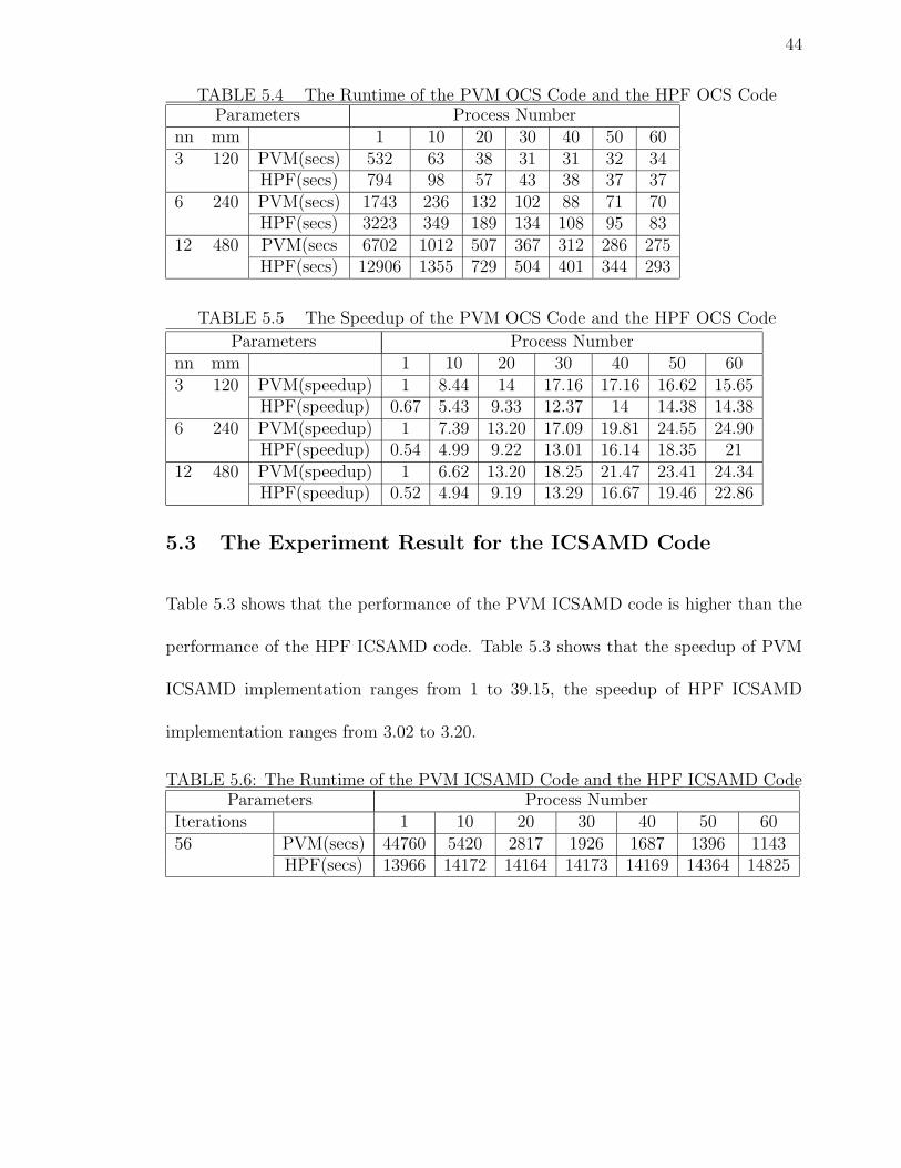
44

TABLE 5.4 The Runtime of the PVM OCS Code and the HPF OCS CodeParameters Process Number

nn mm 1 10 20 30 40 50 603 120 PVM(secs) 532 63 38 31 31 32 34

HPF(secs) 794 98 57 43 38 37 376 240 PVM(secs) 1743 236 132 102 88 71 70

HPF(secs) 3223 349 189 134 108 95 8312 480 PVM(secs 6702 1012 507 367 312 286 275

HPF(secs) 12906 1355 729 504 401 344 293

TABLE 5.5 The Speedup of the PVM OCS Code and the HPF OCS Code

Parameters Process Numbernn mm 1 10 20 30 40 50 603 120 PVM(speedup) 1 8.44 14 17.16 17.16 16.62 15.65

HPF(speedup) 0.67 5.43 9.33 12.37 14 14.38 14.386 240 PVM(speedup) 1 7.39 13.20 17.09 19.81 24.55 24.90

HPF(speedup) 0.54 4.99 9.22 13.01 16.14 18.35 2112 480 PVM(speedup) 1 6.62 13.20 18.25 21.47 23.41 24.34

HPF(speedup) 0.52 4.94 9.19 13.29 16.67 19.46 22.86

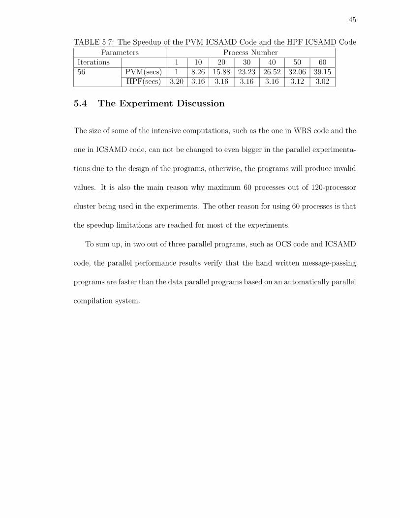
5.3 The Experiment Result for the ICSAMD Code

Table 5.3 shows that the performance of the PVM ICSAMD code is higher than the

performance of the HPF ICSAMD code. Table 5.3 shows that the speedup of PVM

ICSAMD implementation ranges from 1 to 39.15, the speedup of HPF ICSAMD

implementation ranges from 3.02 to 3.20.

TABLE 5.6: The Runtime of the PVM ICSAMD Code and the HPF ICSAMD CodeParameters Process Number

Iterations 1 10 20 30 40 50 6056 PVM(secs) 44760 5420 2817 1926 1687 1396 1143

HPF(secs) 13966 14172 14164 14173 14169 14364 14825

45

TABLE 5.7: The Speedup of the PVM ICSAMD Code and the HPF ICSAMD Code

Parameters Process NumberIterations 1 10 20 30 40 50 6056 PVM(secs) 1 8.26 15.88 23.23 26.52 32.06 39.15

HPF(secs) 3.20 3.16 3.16 3.16 3.16 3.12 3.02

5.4 The Experiment Discussion

The size of some of the intensive computations, such as the one in WRS code and the

one in ICSAMD code, can not be changed to even bigger in the parallel experimenta-

tions due to the design of the programs, otherwise, the programs will produce invalid

values. It is also the main reason why maximum 60 processes out of 120-processor

cluster being used in the experiments. The other reason for using 60 processes is that

the speedup limitations are reached for most of the experiments.

To sum up, in two out of three parallel programs, such as OCS code and ICSAMD

code, the parallel performance results verify that the hand written message-passing

programs are faster than the data parallel programs based on an automatically parallel

compilation system.

Chapter 6

CONCLUSIONS

6.1 Summary and Conclusions

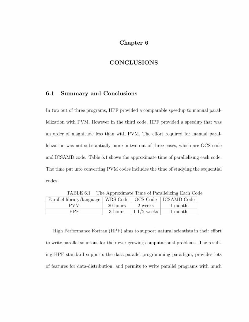
In two out of three programs, HPF provided a comparable speedup to manual paral-

lelization with PVM. However in the third code, HPF provided a speedup that was

an order of magnitude less than with PVM. The effort required for manual paral-

lelization was not substantially more in two out of three cases, which are OCS code

and ICSAMD code. Table 6.1 shows the approximate time of parallelizing each code.

The time put into converting PVM codes includes the time of studying the sequential

codes.

TABLE 6.1 The Approximate Time of Parallelizing Each Code

Parallel library/language WRS Code OCS Code ICSAMD CodePVM 20 hours 2 weeks 1 monthHPF 3 hours 1 1/2 weeks 1 month

High Performance Fortran (HPF) aims to support natural scientists in their effort

to write parallel solutions for their ever growing computational problems. The result-

ing HPF standard supports the data-parallel programming paradigm, provides lots

of features for data-distribution, and permits to write parallel programs with much

47

less programming effort than with standard communication libraries, such as PVM

or MPI. The performance of compiled HPF programs is considered low because of

the communication overhead[15]. The HPF implementation of Portland Group PGI

on the Linux cluster is no exception to this rule.

Even in worse, this experiment suggests that the effort required to understand

the sequential code and HPF language well enough and to select the proper HPF

annotations for the FORTRAN program, can be comparable to the effort required to

rewrite the sequential FORTRAN code into PVM code. Also some knowledge of HPF

compiler techniques might be needed in converting complicated FORTRAN code into

HPF code.

The author’s personal experiences obtained from these six parallel programming

experimentations suggest that HPF does better when parallelizing the operations on

arrays and code structure is simpler. If there are large amounts of the interactions

with user interface devices and (or) subroutine calls in the parallelizing scope, PVM

is likely to be more efficient.

For a scientist, she (or he) can parallelize an application by hand which may

be more complicated but which results in a faster parallel program, or, she (or he)

can use HPF which may be easier to program but which usually results in a slower

runtime.

48

REFERENCES

[1] High Performance Fortran Forum. High Performance Fortran Specification.November 1994.

[2] C. Koelbel, D. Loveman, R. Schreiber, G. Steele Jr., and M. Zosel. The High

Performance Fortran Handbook. The MIT Press,1994.

[3] H. Zima, H.-J. Bast, and M. Gerndt. “SUPERB: A tool for semi-automaticMIMD/SIMD parallelization.” Parallel Computing, vol.6(1), pp.1–18, 1988.

[4] C. Koelbel, D. Loveman, R. Schreiber, G. Steele Jr., and M. Zosel. The High

Performance Fortran Handbook. The MIT Press,1994.

[5] I. Foster, D. Kohr,Jr., R. Krishnaiyer, A. Choudhary. Double Standards: Bring-ing Task Parallelism to HPF via the Message Passing Interface.http://citeseer.ist.psu.edu/foster96double.html

[6] The Portland Group, Inc. PGHPF User’s Guide.http://www.pgroup.com/hpf docs/pghpf ug/hpfug.htm.

[7] The Portland Group, Inc. PGHPF User’s Guide.http://www.pgroup.com/hpf docs/pghpf ug/hpfug.htm.

[8] P. Merkey. Beowulf History.http://wwww.beowulf.org/beowulf/history.html.

[9] B. Zubik-Kowal. Error Bounds for Spatial Discretization and Waveform Re-

laxation Applied to Parabolic Functional Differential Equations. J. Math. Anal.Appl. 293 (2004), No. 2, pp.496–510.

[10] J. L. Mead. Assimilation of Simulated Float Data in Lagrangian Coordinates. InPress Ocean Modeling, 2004.

[11] P. S. Routh, D. W. Oldenburg. Inversion of Controlled Source Audio-Frequency

Magnetotelluric Data for a Horizontally Layered Earth. Geophysics, 64, No. 6,pp 1689–1697.

[12] B. Wilkinson, M. Allen. Parallel Programming. pp.40, Prentice-Hall, Inc., 1999.

[13] B. Wilkinson, M. Allen. Parallel Programming. pp. 11, Prentice-Hall, Inc., 1999.

49

[14] High Performance Fortran Forum. High Performance Fortran Specification. Ver-sion 1.0, May 3, 1993.

[15] M.Muller, F. Informatik. About the Performance of HPF: Improving Runtime onthe Cray T3E with Hardware Specific Properties.http://www.ipd.uka.de/mitarbeiter/muellerm/publications/cug2002.pdf.

[16] PVM Home Page: http://www.csm.ornl.gov/pvm/pvm home.html.

50

Appendix A

THE SKETCH CODES IN CHAPTER 2

A.1 Sketch Code: the Quadruply-Nested Iterations in theSequential WRS Code in FORTRAN 90

!

! Code is omitted.

!

DO 200 K=1, MK+1

!

! Code is omitted.

!

DO 600 J=0, M1-1

!

! Code is omitted.

!

DO 3 I=1,N-1

q=1/(qq-H0*(DM(I,I,M)+1.0d0-VS(I,J+1-MC)))

VN(I,J+1)=0.0d0

DO 4 II=1, N-1

!

! Code is omitted.

!

4 END DO

VN(I,J+1)=VN(I,J+1)+(DM(I,0,M)+DM(I,N,M))*tt*e

VN(I,J+1)=VN(I,J+1)*H0

VN(I,J+1)=VN(I,J+1)+3*VN(I,J)-1.5d0*VN(I,J-1) &

& +VN(I,J-2)/3.0d0

VN(I,J+1)=VN(I,J+1)*q

3 END DO

600 END DO

!

! Code is omitted.

!

200 END DO

51

A.2 Sketch Code: the Doubly-Nested Loops in the Sequen-tial OCS Code in FORTRAN 90

do 1000 n=1,nn

!

! Code is omitted.

!

do 2000 m=1,mm

!

! Initialize the impulse, then find it for the mth representer.

!

fh=0.d0

flam=0.d0

fth=0.d0

call impulse(NI,NJ,NK,mm,m,m,i_pos,j_pos,k_pos,bhat,

1 fh,flam,fth)

!

! Initialize the solution from the adjoint model, then find it.

!

hnm1=0.d0

lamnm1=0.d0

thnm1=0.d0

h=0.d0

lam=0.d0

th=0.d0

call adjLmodel(NI,NJ,NK,dalp,dbet,dt,tt,fh,flam,fth,

1 lamnm1,thnm1,h,lam,th)

!

! Initialize the weights in the forward representer model, then find it.

!

flam=0.d0

fth=0.d0

call weights(NI,NJ,NK,dalp,dbet,dt,lamnm1,thnm1,

1 lam,th,flint,ftint,flpint,ftpint,flam,fth)

!

! Initialize the representer solution, then find it.

!

h=0.d0

lam=0.d0

th=0.d0

call oceLmodel(NI,NJ,NK,dalp,dbet,dt,tt,flint,ftint,

52

1 flpint,ftpint,flam,fth,zeros,zeros,zeros,h,lam,th)

!

! Put the mth representer solution in the mth row of the representer matrix.

!

forall (i=1:mm/3)

1 rr(m,i)=lam(i_pos(i),j_pos(i),k_pos(i))

forall (i=1:mm/3)

1 rr(m,mm/3+i)=th(i_pos(i),j_pos(i),k_pos(i))

forall (i=1:mm/3)

1 rr(m,2*mm/3+i)=h(i_pos(i),j_pos(i),k_pos(i))

2000 end do

1000 end do

A.3 Sketch Code: the Single Loop in Subroutine data inputin the Sequential ICSAMD Code in FORTRAN 77

c

c Main program

c

call data_input

stop

end

c

c Subroutine data_input

c


c

c Variable declarations are omitted.

c

c Start of data input to the program and allocate memory for arrays

c and matrices.

c

c Each iteration does the inversion computation and store the result

c in the output files

c

c nstn = 56

c

do IRECV = 1, nstn

c

c Omit the code for data assignment

53

c

call invert (

1 nfreq,freq_array,ndata,dobs,sd,dpred,

1 INVFLAG,DATFLAG,nl,sref,depth,

1 sigma0,hh,chifact,misfact,alpha_s,

1 alpha_z,niter,mis_exa,mis_exp,mis_eya,mis_eyp,

1 mis_hxa,mis_hxp,mis_hya,mis_hyp,mis_rxy,mis_pxy,

1 mis_ryx,mis_pyx,mis_hza,mis_hzp)

c

c Update the output files

c

end do

c

c Free the memory of arrays and matrices and close the files

c

return

end

c

c All other subroutines and functions are omitted here.

c

54

Appendix B

PVM IMPLEMENTATIONS IN CHAPTER 3

B.1 PVM Implementation on WRS Code

B.1.1 The Makefile.aimk of PVM WRS Code

SHELL = /bin/sh

PVMDIR = $(HOME)/pvm3

SDIR = $(PWD)/..

BDIR = $(HOME)/pvm3/bin

XDIR = $(BDIR)/$(PVM_ARCH)

FC = pgf90

DEBUGON = -D DEBUG

CFLOPTS = -O -Wall

CFLAGS = $(CFLOPTS) -I$(PVM_ROOT)/include $(ARCHCFLAGS)

PVMLIB = -lpvm3

PVMHLIB = -lpvm3

OBJECTS = timing.o

LIBS = $(PVMLIB) $(ARCHLIB)

HLIBS = $(PVMHLIB) $(ARCHLIB)

GLIBS = -lgpvm3

FORT = pgf90

FFLOPTS = -fast -Mextend

FFLAGS = $(FFLOPTS) $(ARCHFFLAGS)

FLIBS = -lfpvm3

LFLAGS = $(LOPT) -L$(PVM_ROOT)/lib/$(PVM_ARCH)

FPROGS = cl2$(EXESFX)

default: cl2$(EXESFX)

all: f-all

f-all: $(FPROGS)

clean:

rm -f ~/*.out ~/*.dat

rm -f $(PWD)/cl2.o w.o shift.o

rm -f $(HOME)/pvm3/bin/LINUXI386/$(FPROGS)

55

$(XDIR):

- mkdir $(BDIR)

- mkdir $(XDIR)

cl2$(EXESFX): $(SDIR)/cl2.f $(SDIR)/w.f $(SDIR)/shift.f $(XDIR) $(OBJECTS)

$(FORT) $(FFLAGS) -o $@ $(SDIR)/cl2.f $(SDIR)/w.f \

$(SDIR)/shift.f $(LFLAGS) $(OBJECTS) $(FLIBS) $(GLIBS) $(LIBS)

mv $@ $(XDIR)

B.1.2 The WRS Sketch Code in PVM with Slow Speed

!

! Enroll in PVM and get my TID.

!

call pvmfmytid(my_tid)

!

! Determine the size of my sibling list.

!

call pvmfsiblings(ntids, -1, idum)

IF (ntids .gt. MAXNPROC) ntids = MAXNPROC

DO I=0, ntids-1

call pvmfsiblings(ntids, I,tids(I))

END DO

!

! Assign number to each process.

!

me = 0

DO I=0, ntids-1

IF(tids(I).EQ.my_tid) THEN

me = I

EXIT

END IF

END DO

!

! All processes join the group ‘‘cl’’.

!

call pvmfjoingroup(’cl’, numt )

IF( numt .lt. 0 ) THEN

call pvmfperror( ’joingroup: ’, my_info)

call pvmfexit( my_info )

56

stop

END IF

call pvmffreezegroup(’cl’,ntids,my_info)

!

! Data patitioning zone, detailed code is omitted.

!

!

! The following is the outermost loop calculations.

!

DO K=1,MK+1

!

! The following is the second inner loop calculations.

!

DO J=0,M1-1

!

! Some data calculations is omitted here.

!

! In the following third inner loop, for each iteration, the

! calculations of one column of the matrix is parallelized.

!

IF(me .EQ. 0)THEN

DO s=1,ntids-1

call pvmfrecv(-1, msgtag_1, my_info)

call pvmfunpack(integer4,mm, 1, 1, my_info)

call pvmfunpack(integer4,kk, 1, 1, my_info)

call pvmfunpack(real8,VN(mm:kk,J+1),(kk-mm+1),1,my_info)

END DO

ELSE

!

! The slaves compute their own shares of one column of the matrix VN

! and send results back to the master

!

DO I=mm,kk

!

! Initialize data.

!

! The forth inner loop calculations

!

! The computation of matrix VN

!

END DO

57

call pvmfinitsend(PVMDATARAW, my_info)

call pvmfpack(integer4,mm, 1, 1, my_info)

call pvmfpack(integer4,kk, 1, 1, my_info)

call pvmfpack(real8,VN(mm:kk,J+1),(kk-mm+1),1,my_info)

call pvmfsend(tids(0), msgtag_1, my_info)

END IF

!

! Process synchronization

!

call pvmfbarrier(’cl’,ntids, my_info )

END DO

!

! After all processes exit the second inner loop, the master process

! broadcasts final result to all slaves.

!

IF(me .EQ.0)THEN


call pvmfpack(real8,vs(1,1),(N+1)*(M1+MC3+1),1,my_info)

call pvmfbcast(’cl’, msgtag_2,my_info)

ELSE

call pvmfrecv(tids(0), msgtag_2, my_info)

call pvmfunpack(real8,vs(1,1),(N+1)*(M1+MC3+1),1,my_info)

END IF


END DO

call pvmfbarrier(’cl’,ntids, my_info)

!

! All processes leave the group ‘‘cl’’.

!

call pvmflvgroup( ’cl’, my_info)

!

! PVM exits.

!

call PVMFEXIT(my_tid)

stop

END

58

B.1.3 The WRS Sketch Code in PVM with Fast Speed

!

! The following code only include the quadruply-nested loops, the rest part

! is the same as the code in Appendix B.1.2.

!

! The outermost loop

!

DO K=1,MK+1

!

! Some data calculations is omitted here.

!

!

! The following is the second inner loop computation which is parallelized.

!

IF(me .EQ. 0)THEN

!

! The master colloects a share of rows of the matrix VN from each slave.

!

DO s=1,ntids-1

VT=0.0d0


call pvmfunpack(integer4,mm, 1, 1, my_info)

call pvmfunpack(integer4,kk, 1, 1, my_info)

call pvmfunpack(real8, VT(0:(M1-1),mm),(kk-mm+1)*(M1+MC3 +1), &

& 1,my_info)

DO I=mm,kk

DO J=0,M1-1

VN(I,J+1) = VT(J,I)

END DO

END DO

END DO

ELSE

!

! The slaves compute their own shares of the matrix and send results to

! the master.

!

DO 3 I=mm,kk

DO 601 J=0,M1-1

!

! Initialize data.

59

!

! The forth inner loop calculations

!

! The computation of matrix VN

!

601 END DO

3 END DO


call pvmfpack(integer4,mm, 1, 1, my_info)

call pvmfpack(integer4,kk, 1, 1, my_info)

call pvmfpack(real8, VT(0:(M1-1),mm),(kk-mm+1)*(M1+MC3+1),1,my_info)


END IF

!

! Prcess synchronization

!


!

! The master process broadcasts final result to all slaves.

!

IF(me .EQ.0)THEN


call pvmfpack(real8,vs(1,1),(N+1)*(M1+MC3+1),1,my_info)

call pvmfbcast(’cl’, msgtag_2,my_info)

ELSE


call pvmfunpack(real8,vs(1,1),(N+1)*(M1+MC3+1),1,my_info)

END IF

!

! Prcess synchronization

!


END DO

B.2 PVM Implementation on OCS Code

B.2.1 The Makefile.aimk of PVM OCS Code

SHELL = /bin/sh


60

SDIR = $(PWD)/..



FC = pgf90

DEBUGON = -D DEBUG

CFLOPTS = -O -Wall


PVMLIB = -lpvm3

PVMHLIB = -lpvm3

OBJECTS = timing.o



GLIBS = -lgpvm3

FORT = pgf90

FFLOPTS = -fast -Mextend


FLIBS = -lfpvm3


FPROGS = figure10$(EXESFX)

default: figure10$(EXESFX)

all: f-all

f-all: $(FPROGS)

clean:

rm -f ~/*.out ~/*.dat

rm -f $(PWD)/figure10.o dgefa.o dgesl.o

rm -f $(HOME)/pvm3/bin/LINUXI386/*.dat

rm -f $(HOME)/pvm3/bin/LINUXI386/*.out


$(XDIR):

- mkdir $(BDIR)

- mkdir $(XDIR)

figure10$(EXESFX): $(SDIR)/figure10.f $(SDIR)/dgefa.f $(SDIR)/dgesl.f \

$(XDIR) $(OBJECTS)

$(FORT) $(FFLAGS) -o $@ $(SDIR)/figure10.f $(SDIR)/\

dgefa.f $(SDIR)/dgesl.f $(LFLAGS) $(OBJECTS) $(FLIBS)\

$(GLIBS) $(LIBS)

mv $@ $(XDIR)

61

B.2.2 The OCS Sketch Code in PVM

!

! Enroll in PVM and get my TID

!


!

! Determine the size of my sibling list

!


IF (ntids .gt. MAXNPROC) ntids = MAXNPROC

DO I=0, ntids-1


END DO

!

! Assign number to each process

!

me = 0

DO I=0, ntids-1


me = I

EXIT

END IF

END DO

!

! All processes join the group ‘‘figure10’’

!

call pvmfjoingroup(’figure10’, numt )

IF( numt .lt. 0 ) THEN



stop

END IF

call pvmffreezegroup(’figure10’,ntids,my_info)

!

! Code is omitted

!

!

! All processes start the outermost iteration.

!

DO 1000 n=1,nn

62

!

! Code is omitted

!

call pvmfbarrier(’figure10’,ntids, my_info )

!

! The master process receives the partial solutions from slaves

!

IF(me .EQ. 0)THEN

DO 2000 q=1,mm

m, h, lam, th = 0


call pvmfunpack(integer4,m, 1, 1, my_info)

call pvmfunpack(real8,h(1,1,1), NI*NJ*NK, 1, my_info)

call pvmfunpack(real8,lam(1,1,1), NI*NJ*NK, 1, my_info)

call pvmfunpack(real8,th(1,1,1), NI*NJ*NK, 1, my_info)

!

! The master put the mth representer solution in the mth row of the

! representer matrix.

!

forall (i=1:mm/3)

1 rr(m,i)=lam(i_pos(i),j_pos(i),k_pos(i))

forall (i=1:mm/3)

1 rr(m,mm/3+i)=th(i_pos(i),j_pos(i),k_pos(i))

forall (i=1:mm/3)

1 rr(m,2*mm/3+i)=h(i_pos(i),j_pos(i),k_pos(i))

2000 END DO

!

! The master process sends the final results to all slaves.

!


call pvmfpack(real8,rr(1,1), mm*mm, 1, my_info)

call pvmfbcast(’figure10’, msgtag_2,my_info)

ELSE

!

! Data Partittion part for slave processes is omitted.

!

!

! The slave process calculates its own share of matrix

!

DO m=j, k

!

! Initialize the impulse, then find it for the mth representer.

63

! The code on data initialization is omitted.

!

call impulse(...)

!

! Initialize the solution from the adjoint model, then find it.

! Thecode on data initialization is omitted.

!

call adjLmodel(..)

!

! Initialize the weights in the forward representer model, then find it.


call weights(..)

!

! Initialize the representer solution, then find it.


!

call oceLmodel(..)

!

! The slave sends data back to the master process.

!


call pvmfpack(integer4,m, 1, 1, my_info)

call pvmfpack(real8,h(1,1,1), NI*NJ*NK, 1, my_info)

call pvmfpack(real8,lam(1,1,1), NI*NJ*NK, 1, my_info)

call pvmfpack(real8,th(1,1,1), NI*NJ*NK, 1, my_info)


END DO

!

! The slave receives the final result from the master process.

!

call pvmfrecv(tids(0),msgtag_2, my_info)

call pvmfunpack(real8,rr(1,1), mm*mm, 1, my_info)

END IF

!

! Process sychronization

!

call pvmfbarrier(’figure10’,ntids, my_info)

!

! The code for outermost loop is omitted.

!

1000 END DO

!

64

! All processes exit PVM.

!

call pvmfbarrier(’figure10’,ntids, my_info)

call pvmflvgroup( ’figure10’, my_info)

call PVMFEXIT(my_tid)

!

! The end of the program

!

stop

end

!

! All other subroutines are omitted here.

!

B.3 PVM Implementation on ICSAMD Code

B.3.1 The Makefile.aimk of PVM ICSAMD Code

SHELL = /bin/sh


SDIR = $(PWD)/..



FC = pgf77

DEBUGON = -D DEBUG

CFLOPTS = -O -Wall


PVMLIB = -lpvm3

PVMHLIB = -lpvm3

OBJECTS = timing.o



GLIBS = -lgpvm3

FORT = pgf77

FFLOPTS = -fast -Kieee -pc 64


FLIBS = -lfpvm3


FPROGS = csamt_latest$(EXESFX)

65

default: csamt_latest$(EXESFX)

all: f-all

f-all: $(FPROGS)

clean:

rm -f $(HOME)/chisq.log $(HOME)/fit.dat\

$(HOME)/inv_model.plt $(HOME)/model.norm\

$(HOME)/JTJ.dat $(HOME)/G.dat\

$(HOME)/J.dat $(HOME)/modeliter\

$(HOME)/csamt.log $(HOME)/csamt.con\

$(HOME)/pred_exa.dat $(HOME)/pred_exp.dat\

$(HOME)/pred_eya.dat $(HOME)/pred_eyp.dat\

$(HOME)/pred_hxa.dat $(HOME)/pred_hxp.dat\

$(HOME)/pred_hya.dat $(HOME)/pred_hyp.dat\

$(HOME)/pred_rho_xy.dat $(HOME)/pred_phs_xy.dat\

$(HOME)/pred_rho_yx.dat $(HOME)/pred_phs_xy.dat\

$(HOME)/pred_hza.dat $(HOME)/pred_hzp.dat\

rm -f $(PWD)/\

csamt_latest.o\

uselam_fields.o \

dsvd.o \

qromb.o \

trapzd.o \

polint.o \

sort3.o \

indexx.o \

rminmax.o \

dfcz.o \

dromb2.o \

tranz.o \

dbitrv.o \

dfixrl.o \

drsple.o \

hankz.o \

wts1.o \

dcool2.o \

dfour2.o \

66

drspln.o \

lamda.o \

wts.o \

rtbis.o \

tran.o \

hank.o \

dfconv.o

rm -f $(HOME)/pvm3/bin/LINUXI386/*.dat

rm -f $(HOME)/pvm3/bin/LINUXI386/*.out


$(XDIR):

- mkdir $(BDIR)

- mkdir $(XDIR)

csamt_latest$(EXESFX): $(SDIR)/csamt_latest.f \

$(SDIR)/uselam_fields.f $(SDIR)/dsvd.f \

$(SDIR)/qromb.f $(SDIR)/trapzd.f \

$(SDIR)/polint.f $(SDIR)/sort3.f \

$(SDIR)/indexx.f $(SDIR)/rminmax.f \

$(SDIR)/dfcz.f $(SDIR)/dromb2.f \

$(SDIR)/tranz.f $(SDIR)/dbitrv.f \

$(SDIR)/dfixrl.f $(SDIR)/drsple.f \

$(SDIR)/hankz.f $(SDIR)/wts1.f\

$(SDIR)/dcool2.f $(SDIR)/dfour2.f \

$(SDIR)/drspln.f $(SDIR)/lamda.f \

$(SDIR)/wts.f $(SDIR)/rtbis.f \

$(SDIR)/tran.f $(SDIR)/hank.f \

$(SDIR)/dfconv.f $(XDIR)

$(FORT) $(FFLAGS) -o $@ $(SDIR)/csamt_latest.f \

$(SDIR)/uselam_fields.f $(SDIR)/dsvd.f \

$(SDIR)/qromb.f $(SDIR)/trapzd.f \

$(SDIR)/polint.f $(SDIR)/sort3.f \

$(SDIR)/indexx.f $(SDIR)/rminmax.f \

$(SDIR)/dfcz.f $(SDIR)/dromb2.f \

$(SDIR)/tranz.f $(SDIR)/dbitrv.f \

$(SDIR)/dfixrl.f $(SDIR)/drsple.f \

$(SDIR)/hankz.f $(SDIR)/wts1.f\

$(SDIR)/dcool2.f $(SDIR)/dfour2.f \

$(SDIR)/drspln.f $(SDIR)/lamda.f \

67

$(SDIR)/wts.f $(SDIR)/rtbis.f \

$(SDIR)/tran.f $(SDIR)/hank.f \

$(SDIR)/dfconv.f $(LFLAGS) $(FLIBS) $(GLIBS) $(LIBS)

mv $@ $(XDIR)

B.3.2 The ICSAMD Sketch Code in PVM

c=====================================================================

c The main program

c=====================================================================

include ’/usr/share/pvm3/include/fpvm3.h’

c=====================================================================

c Start parallel routine

c=====================================================================

integer MAXNPROC,my_info

parameter (MAXNPROC = 120)

integer tids(0:MAXNPROC-1),ntids,me,my_tid,idum,numt

c=====================================================================

c Enroll in PVM and get my TID

c=====================================================================


c=====================================================================

c Determine the size of my sibling list

c=====================================================================


if (ntids .GT. MAXNPROC) ntids = MAXNPROC

DO I=0, ntids-1


END DO

me = 0

DO I=0, ntids-1


me = I

END IF

END DO

call pvmfjoingroup(’csamt’, numt )

if( numt .lt. 0 ) then

68



stop

endif

call pvmffreezegroup(’csamt’,ntids,my_info)

call data_input(me, ntids, my_tid,tids,MAXNPROC)

c===================================================================

c Exiting PVM

c===================================================================

call pvmfbarrier(’csamt’,ntids, my_info)

call pvmflvgroup( ’csamt’, my_info)

call pvmfexit(my_tid)

stop

end

c*******************************************************************

c

c INPUT SUBROUTINE TO PASS PARAMETERS TO MAIN PROGRAM (parallel)

c

c*******************************************************************

subroutine data_input (me, ntids, my_tid, tids,MAXNPROC)

include ’/usr/share/pvm3/include/fpvm3.h’

c==================================================================

c Variable declarations...omitted.

c==================================================================

C******************************************************************

C................ START OF DATA INPUT TO THE PROGRAM .............*

C******************************************************************

c==================================================================

c Only process 0 (master) does the job of openning the input

c files and reading data.

c==================================================================

if (me .eq.0) then

OPEN(UNIT=10,FILE=’csamt.inp’,STATUS=’OLD’)

c==================================================================

c The codes on reading files are omitted

69

c==================================================================

c==================================================================

c Process 0 sends data it read from csamt.inp and file1 to

c process 1,2 ... nproc-1

c==================================================================


call pvmfpack(integer4,niter, 1, 1, my_info)

call pvmfpack(real8,chifact,1,1,my_info)

call pvmfpack(real8,misfact,1,1,my_info)

call pvmfpack(integer4, INVFLAG,1,1,my_info)

call pvmfpack(integer4 ,DATFLAG,1,1,my_info)

call pvmfpack(integer4, IREF,1,1,my_info)

call pvmfpack(real8,alpha_s,1,1,my_info)

call pvmfpack(real8,alpha_z,1,1,my_info)

call pvmfpack(integer4, nfmax,1,1,my_info)

call pvmfpack(real8,xc1,1,1,my_info)

call pvmfpack(real8,yc1,1,1,my_info)

call pvmfpack(real8,xc2,1,1,my_info)

call pvmfpack(real8,yc2,1,1,my_info)

call pvmfpack(integer4, nstn,1,1,my_info)

call pvmfbcast(’csamt’, msgtag_2,my_info)

else

c===================================================================

c Process 1 to nproc-1 receive data from process 0

c===================================================================


call pvmfunpack(integer4,niter, 1, 1, my_info)

call pvmfunpack(real8,chifact,1,1,my_info)

call pvmfunpack(real8,misfact,1,1,my_info)

call pvmfunpack(integer4, INVFLAG,1,1,my_info)

call pvmfunpack(integer4 ,DATFLAG,1,1,my_info)

call pvmfunpack(integer4, IREF,1,1,my_info)

call pvmfunpack(real8,alpha_s,1,1,my_info)

call pvmfunpack(real8,alpha_z,1,1,my_info)

call pvmfunpack(integer4, nfmax,1,1,my_info)

call pvmfunpack(real8,xc1,1,1,my_info)

call pvmfunpack(real8,yc1,1,1,my_info)

call pvmfunpack(real8,xc2,1,1,my_info)

call pvmfunpack(real8,yc2,1,1,my_info)

call pvmfunpack(integer4, nstn,1,1,my_info)

70

end if

c====================================================================

c Processes are synchronized

c====================================================================


c===================================================================

c Allocate memory for global variables (code is omitted).

c===================================================================

c===================================================================

c Process 0 continues reading data from file1, file2 and file3

c and sends them to process 1,2...nproc-1 (code is omitted)

c===================================================================

c====================================================================

c Process 1 to nproc-1 receive all data sent from

c process 0(code is omitted).

c====================================================================

c====================================================================

c Processes are synchronized

c====================================================================


c====================================================================

c Process 0 closes file 1,2,3 then open output file 4,7,8,9,10,

c 11,12,13,14,16,17,18,19,20,21,99 (code is omitted)

c====================================================================

C******************************************************************

C.................. END OF DATA INPUT TO THE PROGRAM .............*

C******************************************************************

C******************************************************************

C................. START OF THE INVERSION PROCESS ................*

C******************************************************************

if(me .eq. 0)then

c====================================================================

c Process 0 allocates memory for local variables

71

c ( code is omitted )

c====================================================================

c====================================================================

c Process 0 first sends tasks to all slaves

c====================================================================

ntids_slave = ntids -1

my_count = 0

if(ntids-1 .GT. nstn) then

ntids_slave = nstn

end if

do i=1, ntids_slave


call pvmfpack(integer4,i,1,1,my_info)

call pvmfsend(tids(i), msgtag_10,my_info)

end do

nstn_number = ntids_slave

do while(my_count .NE. (ntids-1))

nstn_number = nstn_number +1

c===================================================================

c Process 0 receives result data from the slave processes

c doing inversion loops

c===================================================================

ptr_sig = MALLOC(8*nl)


call pvmfunpack(integer4,my_meNumber, 1, 1, my_info)

call pvmfunpack(integer4,my_IRECV, 1, 1, my_info)

call pvmfunpack(real8,mis_exa,1,1,my_info)

call pvmfunpack(real8,mis_exp,1,1,my_info)

call pvmfunpack(real8,mis_eya,1,1,my_info)

call pvmfunpack(real8,mis_eyp,1,1,my_info)

call pvmfunpack(real8,mis_hxa,1,1,my_info)

call pvmfunpack(real8,mis_hxp,1,1,my_info)

call pvmfunpack(real8,mis_hya,1,1,my_info)

call pvmfunpack(real8,mis_hyp,1,1,my_info)

call pvmfunpack(real8,mis_rxy,1,1,my_info)

call pvmfunpack(real8,mis_pxy,1,1,my_info)

call pvmfunpack(real8,mis_ryx,1,1,my_info)

call pvmfunpack(real8,mis_pyx,1,1,my_info)

72

call pvmfunpack(real8,mis_hza,1,1,my_info)

call pvmfunpack(real8,mis_hzp,1,1,my_info)

call pvmfunpack(real8,depth(1),nl,1,my_info)

call pvmfunpack(real8,sigma0(1),nl,1,my_info)

call pvmfunpack(real8,xr,1,1,my_info)

call pvmfunpack(integer4,nfreq, 1, 1, my_info)

call pvmfunpack(integer4,ndata, 1, 1, my_info)

ptr_dpred = MALLOC(8*ndata)

ptr_farray = MALLOC(8*nfreq)

ptr_Jac = MALLOC(8*nl*ndata)

ptr_JTJ = MALLOC(8*nl*nl)

ptr_G = MALLOC(8*nl*nl)

call pvmfunpack(real8,dpred(1),ndata,1,my_info)

call pvmfunpack(real8, freq_array(1),nfreq,1,my_info)

call pvmfunpack(real8,Jac(1),nl*ndata,1, my_info)

call pvmfunpack(real8,JTJ(1),nl*nl,1,my_info)

call pvmfunpack(real8,G(1),nl*nl,1,my_info)

c====================================================================

c Process 0 sends new tasks to each slave after the slave

c returned the results of previous task, or sends a terminator

c message to the slave if no more tasks in the ‘‘work pool’’

c====================================================================


if(nstn_number .GT. nstn) then

call pvmfpack(integer4, -1,1,1,my_info)

call pvmfsend(tids(my_meNumber), msgtag_11,my_info)

my_count = my_count +1

else

call pvmfpack(integer4,nstn_number,1,1,my_info)

call pvmfsend(tids(my_meNumber), msgtag_11,my_info)

end if

c==================================================================

c After received the result data from the slave, process 0

c needs to write those data into file 4,7,8,9,10,11,12,13,

c 14,15,16,17,18,19,20,21,99,101,202,and 303( code is ometted).

c==================================================================

c==================================================================

c Process 0 closes file 4,7,8,9,10,11,12,13,14,15,16,17,18,

c 19,20,21,99,101,202,and 303, then free the memory for the

c local variables (code is omitted).

73

c==================================================================

else

c*******************************************************************

c INVERSION LOOP BEGINS HERE. THIS CALLS THE SUBROUINE "INVERT"

c REPEATEDLY FOR EACH STATION.

c*******************************************************************

c===================================================================

c All processes except process 0 parallelize inversion loop

c===================================================================

nstn_number = 0


call pvmfunpack(integer4,nstn_number,1,1,my_info)

IRECV = nstn_number

do while( IRECV .NE. -1)

c===================================================================

c Part of the executable statements are omitted...

c===================================================================

call invert (






1 mis_ryx,mis_pyx,mis_hza,mis_hzp,Jac,JTJ,G)

c====================================================================

c Process 1 to nproc-1 send result data coming out from invert

c subroutine to process 0 in order to store them in appropriate

c place

c====================================================================


call pvmfpack(integer4,me, 1, 1, my_info)

call pvmfpack(integer4,IRECV, 1, 1, my_info)

call pvmfpack(real8,mis_exa,1,1,my_info)

call pvmfpack(real8,mis_exp,1,1,my_info)

call pvmfpack(real8,mis_eya,1,1,my_info)

call pvmfpack(real8,mis_eyp,1,1,my_info)

call pvmfpack(real8,mis_hxa,1,1,my_info)

74

call pvmfpack(real8,mis_hxp,1,1,my_info)

call pvmfpack(real8,mis_hya,1,1,my_info)

call pvmfpack(real8,mis_hyp,1,1,my_info)

call pvmfpack(real8,mis_rxy,1,1,my_info)

call pvmfpack(real8,mis_pxy,1,1,my_info)

call pvmfpack(real8,mis_ryx,1,1,my_info)

call pvmfpack(real8,mis_pyx,1,1,my_info)

call pvmfpack(real8,mis_hza,1,1,my_info)

call pvmfpack(real8,mis_hzp,1,1,my_info)

call pvmfpack(real8,depth(1),nl,1,my_info)

call pvmfpack(real8,sigma0(1),nl,1,my_info)

call pvmfpack(real8,xr,1,1,my_info)

call pvmfpack(integer4,nfreq, 1, 1, my_info)

call pvmfpack(integer4,ndata, 1, 1, my_info)

call pvmfpack(real8,dpred(1),ndata,1,my_info)

call pvmfpack(real8, freq_array(1),nfreq,1,my_info)

call pvmfpack(real8,Jac(1),nl*ndata,1, my_info)

call pvmfpack(real8,JTJ(1),nl*nl,1,my_info)

call pvmfpack(real8,G(1),nl*nl,1,my_info)


c=================================================================

c Free the memory of the local variables ( code is ometted )

c=================================================================

c=================================================================

c The slave receives new task from the master

c=================================================================


call pvmfunpack(integer4,nstn_number,1,1,my_info)

IRECV = nstn_number

end do

end if


C******************************************************************

C................. END OF THE INVERSION PROCESS ................*

C******************************************************************

c==================================================================

c All processes need to deallocate the global variables

75

c ( code is omitted )

c==================================================================


return

end

c==================================================================


c==================================================================

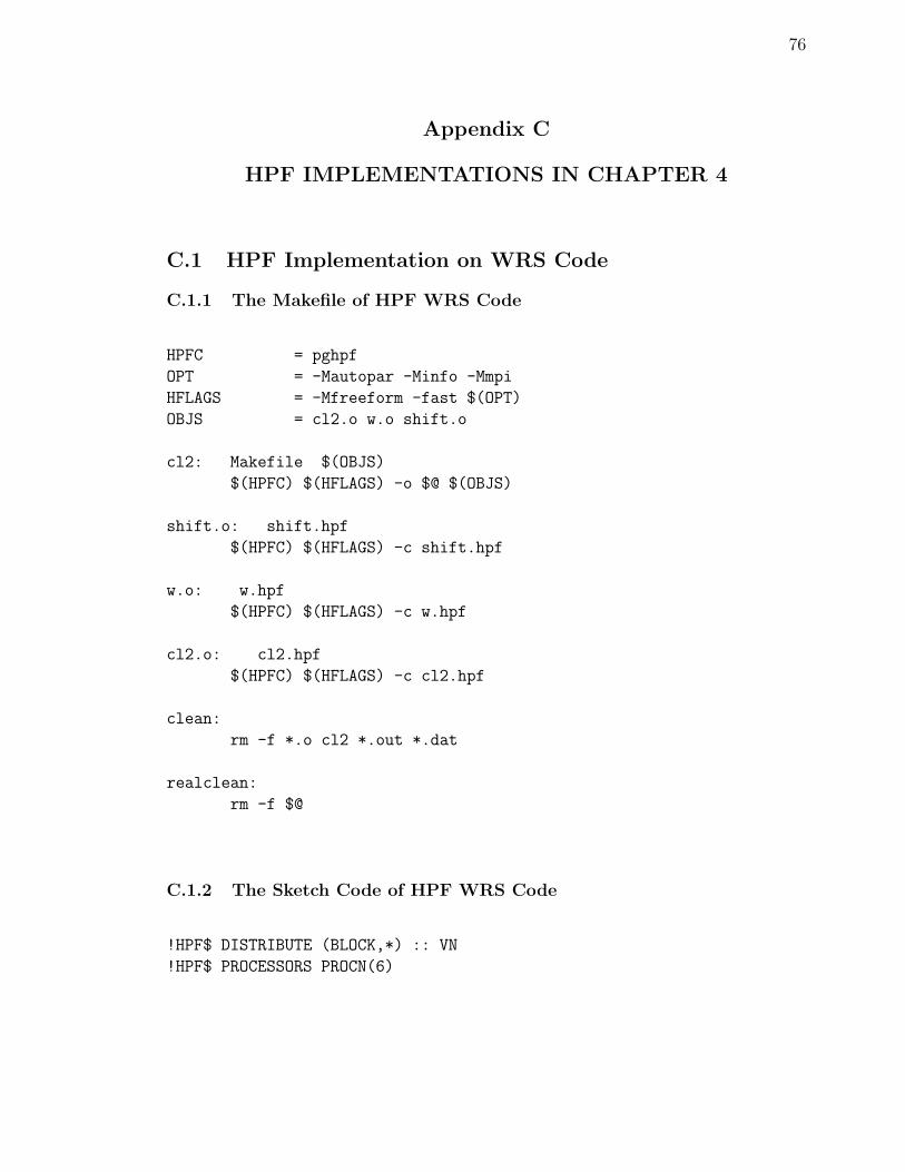
76

Appendix C

HPF IMPLEMENTATIONS IN CHAPTER 4

C.1 HPF Implementation on WRS Code

C.1.1 The Makefile of HPF WRS Code

HPFC = pghpf

OPT = -Mautopar -Minfo -Mmpi

HFLAGS = -Mfreeform -fast $(OPT)

OBJS = cl2.o w.o shift.o

cl2: Makefile $(OBJS)

$(HPFC) $(HFLAGS) -o $@ $(OBJS)

shift.o: shift.hpf

$(HPFC) $(HFLAGS) -c shift.hpf

w.o: w.hpf

$(HPFC) $(HFLAGS) -c w.hpf

cl2.o: cl2.hpf

$(HPFC) $(HFLAGS) -c cl2.hpf

clean:

rm -f *.o cl2 *.out *.dat

realclean:

rm -f $@

C.1.2 The Sketch Code of HPF WRS Code

!HPF$ DISTRIBUTE (BLOCK,*) :: VN

!HPF$ PROCESSORS PROCN(6)

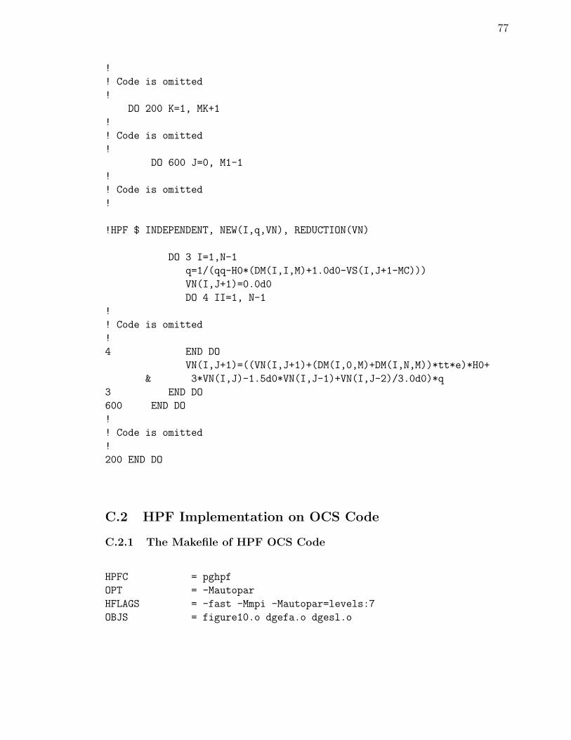
77

!

! Code is omitted

!

DO 200 K=1, MK+1

!

! Code is omitted

!

DO 600 J=0, M1-1

!

! Code is omitted

!

!HPF $ INDEPENDENT, NEW(I,q,VN), REDUCTION(VN)

DO 3 I=1,N-1

q=1/(qq-H0*(DM(I,I,M)+1.0d0-VS(I,J+1-MC)))

VN(I,J+1)=0.0d0

DO 4 II=1, N-1

!

! Code is omitted

!

4 END DO

VN(I,J+1)=((VN(I,J+1)+(DM(I,0,M)+DM(I,N,M))*tt*e)*H0+

& 3*VN(I,J)-1.5d0*VN(I,J-1)+VN(I,J-2)/3.0d0)*q

3 END DO

600 END DO

!

! Code is omitted

!

200 END DO

C.2 HPF Implementation on OCS Code

C.2.1 The Makefile of HPF OCS Code

HPFC = pghpf

OPT = -Mautopar

HFLAGS = -fast -Mmpi -Mautopar=levels:7

OBJS = figure10.o dgefa.o dgesl.o

78

figure10: $(OBJS)


dgefa.o: dgefa.hpf

$(HPFC) $(HFLAGS) -c dgefa.hpf

dgesl.o: dgesl.hpf

$(HPFC) $(HFLAGS) -c dgesl.hpf

figure10.o: figure10.hpf

$(HPFC) $(HFLAGS) -c figure10.hpf

clean:

rm -f *.o figure10 *.out *.dat

realclean:

rm -f $@

C.2.2 The Sketch Code of HPF OCS Code


interface

pure subroutine weights(...)

!

! The scope units are omitted.

!

end subroutine

pure subroutine impulse(...)

!


!

end subroutine

pure subroutine adjLmodel(...)

!


!

79

end subroutine

pure subroutine oceLmodel(...)

!


!

end subroutine

!

! More interface declarations are omitted.

!

end interface

do 1000 n=1,nn

!

! Code is omitted.

!

! Create temporary dummy variables for the subroutine calls

! inside INDEPENDENT loop

!

do i=1,mm/3

temp_i_pos(i) = i_pos(i)

temp_j_pos(i) = j_pos(i)

temp_k_pos(i) = k_pos(i)

end do

my_flint=0.d0

my_ftint=0.d0

my_flpint=0.d0

my_ftpint=0.d0

my_zeros =0.d0

!HPF$ INDEPENDENT

do 2000 m=1,mm

call impulse( NI,NJ,NK,mm,m,m,temp_i_pos,temp_j_pos,temp_k_pos,

1 bhat,fh,flam,fth)

call adjLmodel(NI,NJ,NK,dalp,dbet,dt,tt,fh,flam,fth,

1 lamnm1,thnm1,h,lam,th)

call weights(NI,NJ,NK,dalp,dbet,dt,lamnm1,thnm1,

1 lam,th,my_flint,my_ftint,my_flpint,my_ftpint,flam,fth)

call oceLmodel(NI,NJ,NK,dalp,dbet,dt,tt,my_flint,my_ftint,

80

1 my_flpint,my_ftpint,flam,fth,my_zeros,my_zeros,my_zeros,

1 h,lam,th)

!

! Put the mth representer solution in the mth row of the

! representer matrix.

!

do i=1, mm/3

rr(m,i)=lam(i_pos(i),j_pos(i),k_pos(i))

end do

do i=1,mm/3

rr(m,mm/3+i)=th(i_pos(i),j_pos(i),k_pos(i))

end do

do i=1,mm/3

rr(m,2*mm/3+i)=h(i_pos(i),j_pos(i),k_pos(i))

end do

2000 end do

1000 end do

C.3 HPF Implementation on ICSAMD Code

C.3.1 The Makefile of HPF ICSAMD Code

OBJS = csamt_latest.o uselam_fields.o dsvd.o \

qromb.o trapzd.o polint.o sort3.o \

indexx.o rminmax.o dfcz.o dromb2.o \

tranz.o dbitrv.o dfixrl.o drsple.o \

hankz.o wts1.o dcool2.o dfour2.o \

drspln.o lamda.o wts.o rtbis.o \

tran.o hank.o dfconv.o

HPFC = pghpf

HFLAGS = -Msequence -Mautopar=level:7 -Mmpi -Minfo -Mextend

-Mg -fast -Kieee -pc 64

csamt_latest:$(OBJS)


uselam_fields.o: uselam_fields.hpf

$(HPFC) $(HFLAGS) -c uselam_fields.hpf

dsvd.o: dsvd.hpf

81

$(HPFC) $(HFLAGS) -c dsvd.hpf

qromb.o: qromb.hpf

$(HPFC) $(HFLAGS) -c qromb.hpf

trapzd.o: trapzd.hpf

$(HPFC) $(HFLAGS) -c trapzd.hpf

polint.o: polint.hpf

$(HPFC) $(HFLAGS) -c polint.hpf

sort3.o: sort3.hpf

$(HPFC) $(HFLAGS) -c sort3.hpf

indexx.o: indexx.hpf

$(HPFC) $(HFLAGS) -c indexx.hpf

rminmax.o: rminmax.hpf

$(HPFC) $(HFLAGS) -c rminmax.hpf

dfcz.o: dfcz.hpf

$(HPFC) $(HFLAGS) -c dfcz.hpf

dromb2.o: dromb2.hpf

$(HPFC) $(HFLAGS) -c dromb2.hpf

tranz.o: tranz.hpf

$(HPFC) $(HFLAGS) -c tranz.hpf

dbitrv.o: dbitrv.hpf

$(HPFC) $(HFLAGS) -c dbitrv.hpf

dfixrl.o: dfixrl.hpf

$(HPFC) $(HFLAGS) -c dfixrl.hpf

drsple.o: drsple.hpf

$(HPFC) $(HFLAGS) -c drsple.hpf

hankz.o: hankz.hpf

$(HPFC) $(HFLAGS) -c hankz.hpf

wts1.o: wts1.hpf

82

$(HPFC) $(HFLAGS) -c wts1.hpf

dcool2.o: dcool2.hpf

$(HPFC) $(HFLAGS) -c dcool2.hpf

dfour2.o: dfour2.hpf

$(HPFC) $(HFLAGS) -c dfour2.hpf

drspln.o: drspln.hpf

$(HPFC) $(HFLAGS) -c drspln.hpf

lamda.o: lamda.hpf

$(HPFC) $(HFLAGS) -c lamda.hpf

wts.o: wts.hpf

$(HPFC) $(HFLAGS) -c wts.hpf

rtbis.o: rtbis.hpf

$(HPFC) $(HFLAGS) -c rtbis.hpf

tran.o: tran.hpf

$(HPFC) $(HFLAGS) -c tran.hpf

hank.o: hank.hpf

$(HPFC) $(HFLAGS) -c hank.hpf

dfconv.o: dfconv.hpf

$(HPFC) $(HFLAGS) -c dfconv.hpf

csamt_latest.o: csamt_latest.hpf

$(HPFC) $(HFLAGS) -c csamt_latest.hpf

clean:

/bin/rm -f *.o csamt_latest

C.3.2 The Sketch Code of HPF ICSAMD Code

c=============================================================

c The main program

c=============================================================

83

call data_input

stop

end

c=============================================================

c The subroutine data_input

c=============================================================


integer niter,nl,INVFLAG,DATFLAG,IREF,nstn,MALLOC

integer ndata,ifreq_sum,IZ,kf,nfmax,NFIELD

integer sum_my_nfreq,sum_ndata,my_nfreq,temp_num

integer temp_1, temp_2, mm,tt,k,ii

pointer (ptr_nfreq_stn,nfreq_stn)

pointer (ptr_array_99, array_99)

pointer (ptr_depth_array, depth_array)

pointer (ptr_sigmod_array, sigmod_array)

pointer (ptr_freq_array_array, freq_array_array)

pointer (ptr_dpred_array,dpred_array)

pointer (ptr_ndata_array, ndata_array)

pointer (ptr_Jac_array, Jac_array)

pointer (ptr_JTJ_array, JTJ_array)

pointer (ptr_G_array, G_array)

integer*4 array_99(*), ndata_array(*)

integer*4 nfreq_stn(*)

real*8 depth_array(*), sigmod_array(*)

real*8 freq_array_array(*), dpred_array(*)

real*8 Jac_array(*),JTJ_array(*),G_array(*)

real*8 xr,yr,xc1,yc1,xc2,yc2,misfact,fmin,fmax,chifact

real*8 sig_homo,alpha_s,alpha_z

real*8 mis_exa,mis_exp,mis_eya,mis_eyp

real*8 mis_hxa,mis_hxp,mis_hya,mis_hyp

real*8 mis_rxy,mis_pxy,mis_ryx,mis_pyx

real*8 mis_hza,mis_hzp

pointer (ptr_fstn,fstn),(ptr_xstn,xstn)

pointer (ptr_ystn,ystn),(ptr_sref,sref)

pointer (ptr_Jac, Jac),(ptr_JTJ,JTJ),(ptr_G,G)

84

real*8 fstn(*),xstn(*),ystn(*),sref(*)

real*8 Jac(*),JTJ(*),G(*)

pointer (ptr_sd,sd),(ptr_farray,freq_array)

pointer (ptr_sigmod,sigmod),(ptr_data,data)

pointer (ptr_sig,sigma0),(ptr_dph,depth)

pointer (ptr_hh,hh),(ptr_dobs,dobs)

pointer (ptr_dpred,dpred),(ptr_fitexa,fitexa)

pointer (ptr_fitexp,fitexp),(ptr_fiteya,fiteya)

pointer (ptr_fiteyp,fiteyp),(ptr_fithya,fithya)

pointer (ptr_fithyp,fithyp),(ptr_fithxa,fithxa)

pointer (ptr_fithxp,fithxp),(ptr_fitrxy,fitrxy)

pointer (ptr_fitryx,fitryx),(ptr_fitpxy,fitpxy)

pointer (ptr_fitpyx,fitpyx),(ptr_fithza,fithza)

pointer (ptr_fithzp,fithzp)

real*8 freq_array(*),sigmod(*),data(*),sigma0(*)

real*8 depth(*),hh(*),dobs(*),dpred(*),sd(*)

real*8 fitexa(*),fitexp(*),fiteya(*),fiteyp(*)

real*8 fithxa(*),fithxp(*),fithya(*),fithyp(*)

real*8 fitrxy(*),fitryx(*),fitpxy(*),fitpyx(*)

real*8 fithza(*),fithzp(*)

pointer (ptr_exa_o,exa_o),(ptr_exp_o,exp_o)

pointer (ptr_eya_o,eya_o),(ptr_eyp_o,eyp_o)

pointer (ptr_hxa_o,hxa_o),(ptr_hxp_o,hxp_o)

pointer (ptr_hya_o,hya_o),(ptr_hyp_o,hyp_o)

pointer (ptr_hza_o,hza_o),(ptr_hzp_o,hzp_o)

pointer (ptr_rho_xy,rho_xy),(ptr_phs_xy,phs_xy)

pointer (ptr_rho_yx,rho_yx),(ptr_phs_yx,phs_yx)

pointer (ptr_err_exa,err_exa),(ptr_err_exp,err_exp)

pointer (ptr_err_eya,err_eya),(ptr_err_eyp,err_eyp)

pointer (ptr_err_hxa,err_hxa),(ptr_err_hxp,err_hxp)

pointer (ptr_err_hya,err_hya),(ptr_err_hyp,err_hyp)

pointer (ptr_err_hza,err_hza),(ptr_err_hzp,err_hzp)

pointer (ptr_err_rxy,err_rxy),(ptr_err_pxy,err_pxy)

pointer (ptr_err_ryx,err_ryx),(ptr_err_pyx,err_pyx)

real*8 exa_o(*),exp_o(*),eya_o(*),eyp_o(*)

real*8 hxa_o(*),hxp_o(*),hya_o(*),hyp_o(*)

85

real*8 hza_o(*),hzp_o(*)

real*8 rho_xy(*),rho_yx(*),phs_xy(*),phs_yx(*)

real*8 err_exa(*),err_exp(*),err_eya(*),err_eyp(*)

real*8 err_hxa(*),err_hxp(*),err_hya(*),err_hyp(*)

real*8 err_hza(*),err_hzp(*)

real*8 err_rxy(*),err_ryx(*),err_pxy(*),err_pyx(*)

character*60 file1,file2,file3

CHARACTER*60 INPF

common /loc/xr,yr,xc1,yc1,xc2,yc2

!HPF SEQUENCE:: niter,nl,INVFLAG,DATFLAG,IREF,nstn,MALLOC,

!HPF*ndata,ifreq_sum,IZ,kf,nfmax,NFIELD,sum_my_nfreq,sum_ndata,

!HPF*my_nfreq,temp_num,temp_1, temp_2, mm,tt,k,ii,array_99,

!HPF*ndata_array,nfreq_stn,depth_array, sigmod_array,

!HPF*freq_array_array, dpred_array,Jac_array,JTJ_array,G_array,

!HPF*xr,yr,xc1,yc1,xc2,yc2,misfact,fmin,fmax,chifact,sig_homo,

!HPF*alpha_s,alpha_z,mis_exa,mis_exp,mis_eya,mis_eyp, mis_hxa,

!HPF*mis_hxp,mis_hya,mis_hyp,mis_rxy,mis_pxy,mis_ryx,mis_pyx,

!HPF* mis_hza,mis_hzp,fstn,xstn,ystn,sref,Jac,JTJ,G,freq_array,

!HPF*sigmod,data,sigma0,depth,hh,dobs,dpred,sd,fitexa,fitexp,

!HPF*fiteya,fiteyp,fithxa,fithxp,fithya,fithyp,fitrxy,fitryx,

!HPF*fitpxy,fitpyx,fithza,fithzp,exa_o,exp_o,eya_o,eyp_o,

!HPF*hxa_o,hxp_o,hya_o,hyp_o,hza_o,hzp_o,rho_xy,rho_yx,phs_xy,

!HPF*phs_yx,err_exa,err_exp,err_eya,err_eyp,err_hxa,err_hxp,

!HPF*err_hya,err_hyp,err_hza,err_hzp,err_rxy,err_ryx,err_pxy,

!HPF*err_pyx,/loc/,file1,file2,file3,INPF


c====================================================================

c Interface declarations ( two examples)

c====================================================================

interface

pure subroutine invert (






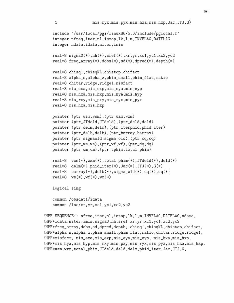
86

1 mis_ryx,mis_pyx,mis_hza,mis_hzp,Jac,JTJ,G)

include ’/usr/local/pgi/linux86/5.0/include/pglocal.f’

integer nfreq,iter,nl,istop,lk,l,m,INVFLAG,DATFLAG

integer ndata,idata,niter,imis

real*8 sigma0(*),hh(*),sref(*),xr,yr,xc1,yc1,xc2,yc2

real*8 freq_array(*),dobs(*),sd(*),dpred(*),depth(*)

real*8 chisq1,chisqNL,chistop,chifact

real*8 alpha_s,alpha_z,phim_small,phim_flat,ratio

real*8 chitar,ridge,ridge1,misfact

real*8 mis_exa,mis_exp,mis_eya,mis_eyp

real*8 mis_hxa,mis_hxp,mis_hya,mis_hyp

real*8 mis_rxy,mis_pxy,mis_ryx,mis_pyx

real*8 mis_hza,mis_hzp

pointer (ptr_wsm,wsm),(ptr_wzm,wzm)

pointer (ptr_JTdeld,JTdeld),(ptr_deld,deld)

pointer (ptr_delm,delm),(ptr_iterphid,phid_iter)

pointer (ptr_delb,delb),(ptr_barray,barray)

pointer (ptr_sigmaold,sigma_old),(ptr_cq,cq)

pointer (ptr_ws,ws),(ptr_wf,wf),(ptr_dq,dq)

pointer (ptr_wm,wm),(ptr_tphim,total_phim)

real*8 wsm(*),wzm(*),total_phim(*),JTdeld(*),deld(*)

real*8 delm(*),phid_iter(*),Jac(*),JTJ(*),G(*)

real*8 barray(*),delb(*),sigma_old(*),cq(*),dq(*)

real*8 ws(*),wf(*),wm(*)

logical sing

common /obsdat1/idata

common /loc/xr,yr,xc1,yc1,xc2,yc2

!HPF SEQUENCE:: nfreq,iter,nl,istop,lk,l,m,INVFLAG,DATFLAG,ndata,

!HPF*idata,niter,imis,sigma0,hh,sref,xr,yr,xc1,yc1,xc2,yc2

!HPF*freq_array,dobs,sd,dpred,depth, chisq1,chisqNL,chistop,chifact,

!HPF*alpha_s,alpha_z,phim_small,phim_flat,ratio,chitar,ridge,ridge1,

!HPF*misfact, mis_exa,mis_exp,mis_eya,mis_eyp, mis_hxa,mis_hxp,

!HPF*mis_hya,mis_hyp,mis_rxy,mis_pxy,mis_ryx,mis_pyx,mis_hza,mis_hzp,

!HPF*wsm,wzm,total_phim,JTdeld,deld,delm,phid_iter,Jac,JTJ,G,

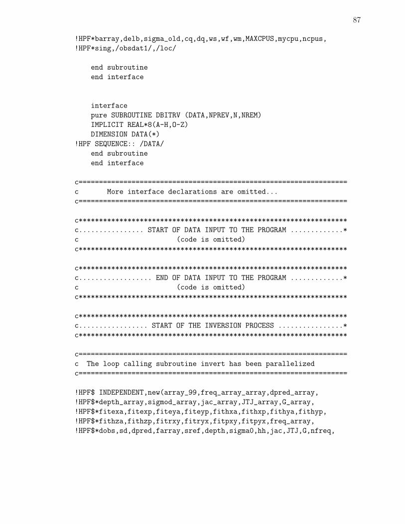
87

!HPF*barray,delb,sigma_old,cq,dq,ws,wf,wm,MAXCPUS,mycpu,ncpus,

!HPF*sing,/obsdat1/,/loc/

end subroutine

end interface

interface

pure SUBROUTINE DBITRV (DATA,NPREV,N,NREM)

IMPLICIT REAL*8(A-H,O-Z)

DIMENSION DATA(*)

!HPF SEQUENCE:: /DATA/

end subroutine

end interface

c==================================================================

c More interface declarations are omitted...

c==================================================================

c******************************************************************

c................ START OF DATA INPUT TO THE PROGRAM .............*

c (code is omitted)

c******************************************************************

c******************************************************************

c.................. END OF DATA INPUT TO THE PROGRAM .............*

c (code is omitted)

c******************************************************************

c******************************************************************

c................. START OF THE INVERSION PROCESS ................*

c******************************************************************

c==================================================================

c The loop calling subroutine invert has been parallelized

c==================================================================

!HPF$ INDEPENDENT,new(array_99,freq_array_array,dpred_array,

!HPF$*depth_array,sigmod_array,jac_array,JTJ_array,G_array,

!HPF$*fitexa,fitexp,fiteya,fiteyp,fithxa,fithxp,fithya,fithyp,

!HPF$*fithza,fithzp,fitrxy,fitryx,fitpxy,fitpyx,freq_array,

!HPF$*dobs,sd,dpred,farray,sref,depth,sigma0,hh,jac,JTJ,G,nfreq,

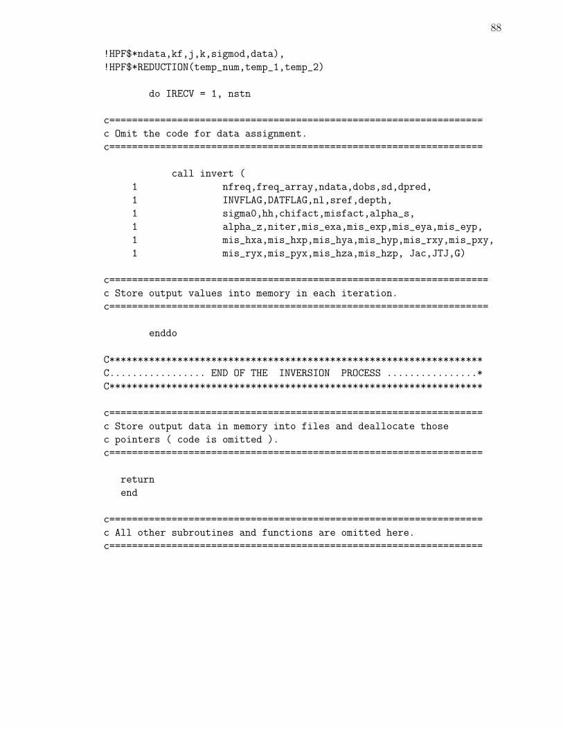
88

!HPF$*ndata,kf,j,k,sigmod,data),

!HPF$*REDUCTION(temp_num,temp_1,temp_2)

do IRECV = 1, nstn

c==================================================================

c Omit the code for data assignment.

c==================================================================

call invert (






1 mis_ryx,mis_pyx,mis_hza,mis_hzp, Jac,JTJ,G)

c===================================================================

c Store output values into memory in each iteration.

c===================================================================

enddo

C******************************************************************

C................. END OF THE INVERSION PROCESS ................*

C******************************************************************

c==================================================================

c Store output data in memory into files and deallocate those

c pointers ( code is omitted ).

c==================================================================

return

end

c==================================================================


c==================================================================

Documents

Manual versus Automatic Parallelization Using PVM and HPF