Embed Size (px)
Citation preview
1
Manufacturing and Rehological Analysis of Spiral Flow Test
Piece
Silas Zewdie Gebrehiwot
Degree Thesis
Plastics Technology
2014

2
DEGREE THESIS Arcada Degree Programme: Plastics Technology
Identification number: 12852
Author: Silas Zewdie Gebrehiwot
Title: Manufacturing and Rheological Analysis of Spiral Flow Test Piece
Supervisor (Arcada): Mathew Vihtonen
Commissioned by:
Abstract:
The spiral flow test is one of the many tests that help to determine the rheological nature of plastics. It is such an important testing method as compared to different testing methods for its help in determining the most critical physical properties of a plastic. The thesis writing is made based on the combination of different course taught in Arcada along with many primary sources focusing on engineering and design of a mould. The spiral flow testing mould is developed with a basic formulation of an Archimedean spiral length. The development of the mould set would be done with the 3D modelling software (SolidWorks). The design is made based on plate standard developed by Hasco. The design of the cavity would have a 4, 25 revolution lengths with a channel diameter of 6 mm. The scope of the thesis is not limited to the design only; rather it actually goes until the complete production of the mould set. Hence, Mastercam simulation would also be made to actually mill the mould plates on the Haas CNC machine in the material science laboratory. The thesis also focuses on doing a virtual injection on Moldflow simulation to reduce manufacturing error and make adjustments before actual part making. Rheological properties mainly focus on a shear viscosity of a molten plastic flow. It is quite a dynamic behaviour that could change with the change in temperature, pressure and injection speed. The thesis would calculate power law index constant for a specific polymer type of Luponen 1840 H LDPE on practical injection process. All of the viscosity analyses performed are based on spiral flow length of plastic travelled under specific operation conditions. Finally, there would be a comparison made between a theoretical formulation, Moldflow simulation and actual injection processes conducted under varying parameters. The thesis would also scientifically explain the reasons for variations.
Key words: Mastercam, Moldflow, Viscosity, Spiral Flow Test, Power
Law Index, Injection Pressure, Rheology
Number of pages:
Language: English
Date of acceptance:
3
TABLE OF CONTENTS
1. INTRODUCTION …………………………………………………………………………………………..…………. 12
1.1. Background ………………………………………………………………………………………………………. 12
1.2. Objectives .……………………………………………………………………………………………………………13
2. LITERATURE REVIEW ……………………………………………………………………………………………… 14
2.1. Injection moulding ……………………………………………………………………………………………… 14
2.1.1. Historical development of injection moulding …………………………………………… 14
2.1.2. Process of injection moulding ………………………………………………… ………………... 15
2.1.3. Injection moulding machine ……………………………………………………… ………….….. 16
2.1.3.1. Injection unit …………………………………………………………………………….………… 16
2.1.3.2. Clamping unit ………………………………………………………………………………….…………. 18
2.1.3.3. Tempering device ………………………………………………………………………………………. 19
2.1.3.4. Control system …………………………………………………………………………………………… 20
2.2. Viscosity ………………………………………………………….……………………………………………….……21
2.2.1. Power law index influence on shear stress versus shear rate graph ………...….23
2.2.2. Carreau’s viscosity model ……………………………………………………………………….…. 23
2.3. Fluid dynamics property of plastics flow ……………………………………………………….… 24
2.3.1. Hagen–Poiseuille equation …………………………………………………………………...…… 25
2.3.2. Pressure versus flow length property for plastics …………………….…………..…… 27
2.4. Archimedean spiral …………………………………………………………………………………………... 29
2.5. Mould design and modelling software ……………………………………………………………. 31
2.6. AutoCAD Moldflow simulation theories and analysis ……………………………………. 32
2.7. Mastercam simulation and HAAS Mill ……………………………………………………………… 34
3. METHOD …………………………………………………………………………………………………………..……… 37
3.1. Archimedean spiral length analysis method ……………………………………..…………... 37
3.2. Isothermal flow analysis method for semi-circular flow channel ……….………... 40
3.3. Power index law method ……………………………………….………………………………………… 43
3.4. Mould design method ………………………….…………………………………………..……………… 43
3.5. Moldflow Simulation analysis on Autodesk Method …………………………………….. 44
3.6. The Mastercam simulation and HAAS mill method …………………….…………………. 45
3.7. Archimedean spiral length calculation ……………………..……………………………..……… 46
3.8. Analysis of flow length versus injection pressure ………………………………….……….. 49
3.8.1. Moldflow simulation pressure versus flow length analysis ………………..………. 49
3.8.2. Theoretical analysis of injection pressure versus flow length …………………….. 51
3.8.3. Practical injection moulding process injection pressure versus
flow length ………………………………………………………………………………………….……… 53
3.9. Viscosity analysis of Luponen 1840 H on practical injection ……….………...…….. 54
4
3.10. Velocity versus viscosity study analysis of practical injection …….………………… 56
3.11. Power law index constant analysis ……………………………………….………………………… 59
3.12. Injection pressure – flow ratio analysis ……………….…………………………………………. 61
4. RESULTS….…………………………………………………………….…………………………………………….……... 63
4.1. Result summary ………………………………………………..………………………………………………… 63
4.1.1. Spiral flow testing mould design ………………………………………………………………… 63
4.1.2. Spiral flow test piece design ………………………………………………………………………. 64
4.1.3. Autodesk Moldflow simulation for plastic injection of the spiral flow
test …………………………………………………………………………………………………………..… 65
4.1.4. Mastercam design and mill for all mould plates …………………………………………. 66
4.1.5. Complete spiral mould set manufacturing …………………………………………………. 68
4.1.6. Isothermal flow formula for semi-circular channel ………………………………… …. 70
4.1.7. Spiral test piece manufacturing ………………………………………………………………….. 71
4.1.8. Comparison of the flow length and injection pressure relationship for
theoretical analysis, Moldflow simulation and practical injection ………………. 72
4.1.9. Comparisons of parametric change influences on viscosity ………………………… 72
4.1.10. Power law index calculation ………………………………………………………………….……. 74
4.1.11. Calibration injection pressure for Luponen 1840 H based on the flow
ratio ………………………………………………………………………………………………………….... 74
4.2. Discussion ………………………………………………………………………….………………………………… 75
4.2.1. Isothermal flow formula ……………………………………………………………………………… 75
4.2.2. Theoretical, simulation and practical injection pressure and
flow length curves ………………………………………………………………………………………. 75
4.2.3. Parametric change influences on viscosity ………………………………………………….. 77
4.2.4. Power law index constant …………………………………………………………….……………. 78
4.2.5. Injection pressure calibration for Luponen 1840 H LDPE …………………..……….. 78
5. CONCLUSION …………………………………………………………………………………………………………….. 79
6. REFERENCE ……………………………………………………………………………..…………………………………. 81
7. APPENDIX I ………………………………………….……………………………………………………………………… 83
8. APPENDIX II …………………………………………………….…………………………………………………………. 86
5
List of figures
Figure 1. Horizontal injection moulding machine layout
Figure 2. Viscosity curve for different polymers and Newtonian fluids
Figure 3. Mean effective pressure versus flow ratio for varying thickness of HDPE
Figure 4. Derivation of the integral formula for arc length
Figure 5. Radius relashionship with X and Y decompostions for included ϴ to calcluate spiral length
Figure 6. Fractional fluid flow analysis on a semi-circular channel
Figure 7. Differential area for semi-circular flow channel
Figure 8. Screenshot of cross-WLF Viscosity model for Luponen 1840 H LDPE
Figure 9. Screenshot of second order Viscosity model for Luponen 1840 H LDPE
Figure 10. Inputs of flow length calculation for the spiral mould cavity
Figure 11. Screenshot for a fill simulation for 10 MPa injection pressure
Figure 12. Screenshot of spiral flow testing mould design
Figure 13. Screenshot of the spiral flow test piece design
Figure 14. Spiral flow test piece design with linear length label
Figure 15. Screenshots of Autodesk fill simulation for varying injection pressure
Figure 16. Screenshot of spiral mould cavity design
Figure 17. Screenshot of Mastercam mill simulation for spiral flow test mould cavity
Figure 18. Screenshot of spiral flow test mould cavity manufacturing
Figure 19. Screenshot of drilling operation performed for cooling channel on mould plates
Figure 20. Screenshot of sprue bushing hole drill
Figure 21. Screenshot of spiral flow testing mould set
Figure 22. Screenshot of a partially assembled spiral flow testing mould
Figure 23. Screenshot of spiral flow test products with varying injection pressure
Figure 24. Screenshot of spiral flow test products with varying injection speed
Figure 25. Comparison of graphs of injection pressure and flow length for theoretical
analysis, Moldflow simulation and practical injection

6
Figure 26. Graph of injection pressure and viscosity curve for practical injection
Figure 27. Graph of Injection speed and viscosity curve for practical injection
Figure 28. Calibration curve of injection pressure for Luponen 1840 H LDPE
Figure 29. Screenshot of Viscosity simulation for Luponen 1840 H LDPE at 100 MPa

7
List of tables
Table 1. Standard plates used to design a spiral flow testing mould
Table 2. Radian conversion to linear length of spiral flow testing with 45 degrees increment
Table 3. Autodesk Moldflow simulation initial parameter settings
Table 4. Autodesk Moldflow fill simulation data for injection pressure variation
Table 5. Theoretical spiral flow length changes for varying injection pressure
Table 6. Injection moulding process parameter for varying injection pressure
Table 7. Spiral flow length changes for varying injection pressure in practical injection moulding
Table 8. Viscosity data of practical injection process for varying injection pressure
Table 9. Injection moulding process parameter for varying injection speed
Table 10. Spiral flow length changes over varying injection speed for practical injection moulding
Table 11. Practical injection process viscosity data for varying injection speed
Table 12. Injection pressure calibration for Luponen 1840 H LDPE spiral flow test
Table 13. Comparison of volume flow rate equations for circular, rectangular and semi-circular
flow channels
8
Glossary
Shear viscosity: fluids’ flow resistance to shearing action
Rheology: a study of fluid flow characterized by temperature, viscosity and pressure variables
Injection moulding: a polymer processing technology carried out by injecting molten plastic into
a mould cavity
Archimedean spiral: a curve generated by a point moving with constant speed along a path
rotating about the origin with a constant rate.
Spiral flow test: a quality validation technique performed by measuring the flow length of a polymer
in a spiral cavity under predefined conditions
Hydraulic pressure: a system of pumping capacity that directly control the injection pressure
Injection pressure: the pressure developed by conversion of a hydraulic pressure by area ratio of
hydraulic system and the screw; and responsible for injection of molten plastic to
mould cavity
Granules: palletized plastic particles produced as raw material for plastic part production
Screw: a part of injection unit the helps to melt and transport plastic from the hopper to nozzle
Shear stress: a stress developed on a surface of an object due to force acting parallel to the
surface
Shear rate: is a rate of shearing measured by the velocity gradient across the radius of a flow
channel
Cooing time: the time taken for an injected molten plastic to solidify down to ejection
temperature level
Newtonian fluid: ideal fluid which has a constant viscosity in its rheological characterization
Shear thinning: rheological tendency of fluids having less viscosity with increased shear stress
Shear thickening: a rheological tendency of fluids showing increased viscosity with increase in
shear stress
Apparent viscosity: a point where a viscosity value needs to be determined
Reference viscosity: a point where a viscosity value is known
Flow length: a length that a molten plastic flows through a mould cavity under predefined set of
conditions
9
Power law index: a constant value denoted by n, that determines the viscosity curve of fluids
Shear force: a force that makes the internal structure of a material to slide one over the other
Axial force: a tensile or compressive action parallel to surface axis
Volume flow rate: a volume of fluid flowing through a certain cross-sectional area per unit time
Flash: quality defect of injection moulding caused by molten plastic leakage through parting line
Parameter: a set of measurable factors defining a certain operation system
Simulation: an abstraction of a real system made to benefit visualizing the real characteristic of an
optimized performance
Velocity/pressure switchover: a point of time reached at which the process monitoring changes
from velocity control to pressure control during Moldflow simulation
Mastercam simulation: a software that gives an option of design, drill, mill and lathe simulation by
generating numerical control machining codes for practical manufacturing
Isothermal condition: operation performed in a system having constant temperature
Mesh: a process of discretizing domain into smaller elements joined by nodes to perform
structural analysis
Calibration: the act of comparing and checking a process with a standard set of parameters.

10
Abbreviation CNC: Computer Numerical Control
ASTM: American Society for Testing and Materials
CROSS-WLF: Cross- (Williams-Landel-Ferry)
LDPE: Low Density Polyethylene
CAD: Computer Aided Design
CAM: Computer Aided Manufacturing
NC: Numerical Control
L/D: Length per Diameter
11
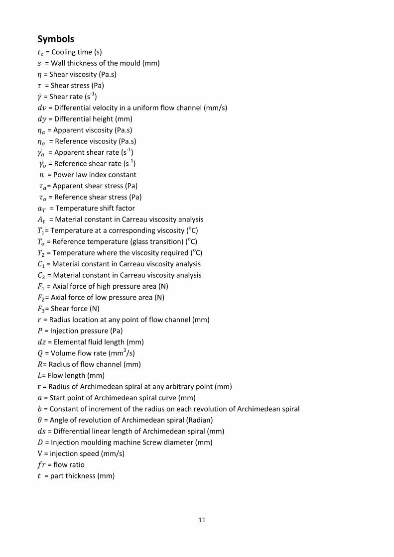
Symbols = Cooling time (s)
= Wall thickness of the mould (mm)
= Shear viscosity (Pa.s)
= Shear stress (Pa)
= Shear rate (s-1)
= Differential velocity in a uniform flow channel (mm/s)
= Differential height (mm)
= Apparent viscosity (Pa.s)
= Reference viscosity (Pa.s)
= Apparent shear rate (s-1)
= Reference shear rate (s-1)
= Power law index constant
= Apparent shear stress (Pa)
= Reference shear stress (Pa)
= Temperature shift factor
= Material constant in Carreau viscosity analysis
= Temperature at a corresponding viscosity (oC)
= Reference temperature (glass transition) (oC)
= Temperature where the viscosity required (oC)
= Material constant in Carreau viscosity analysis
= Material constant in Carreau viscosity analysis
= Axial force of high pressure area (N)
= Axial force of low pressure area (N)
= Shear force (N)
= Radius location at any point of flow channel (mm)
= Injection pressure (Pa)
= Elemental fluid length (mm) = Volume flow rate (mm3/s)
= Radius of flow channel (mm)
= Flow length (mm) = Radius of Archimedean spiral at any arbitrary point (mm)
= Start point of Archimedean spiral curve (mm)
= Constant of increment of the radius on each revolution of Archimedean spiral
= Angle of revolution of Archimedean spiral (Radian)
= Differential linear length of Archimedean spiral (mm)
= Injection moulding machine Screw diameter (mm)
= injection speed (mm/s)
= flow ratio
= part thickness (mm)

12
FORWARD First of all, I would like to thank God for all the strength and blessing he gave me to finish this thesis
work. I would like to acknowledge my supervisor Mr. Mathew Vihtonen for his guidance. Additionally,
I would like to thank Tanja for her support during the whole time I have been doing the thesis. Finally,
I would like to give major credit to Mr. Erland Nyroth. He has been supporting me with all of the
practical CNC milling operations. He has given most of his time diligently for the successful
completion of this thesis work. I would like to recommend upcoming graduates to work with Mr.
Erland and use his potential as resource in their thesis works.
Helsinki, March 2014
Silas Zewdie Gebrehiwot
13
1. INTRODUCTION
1.1 Background
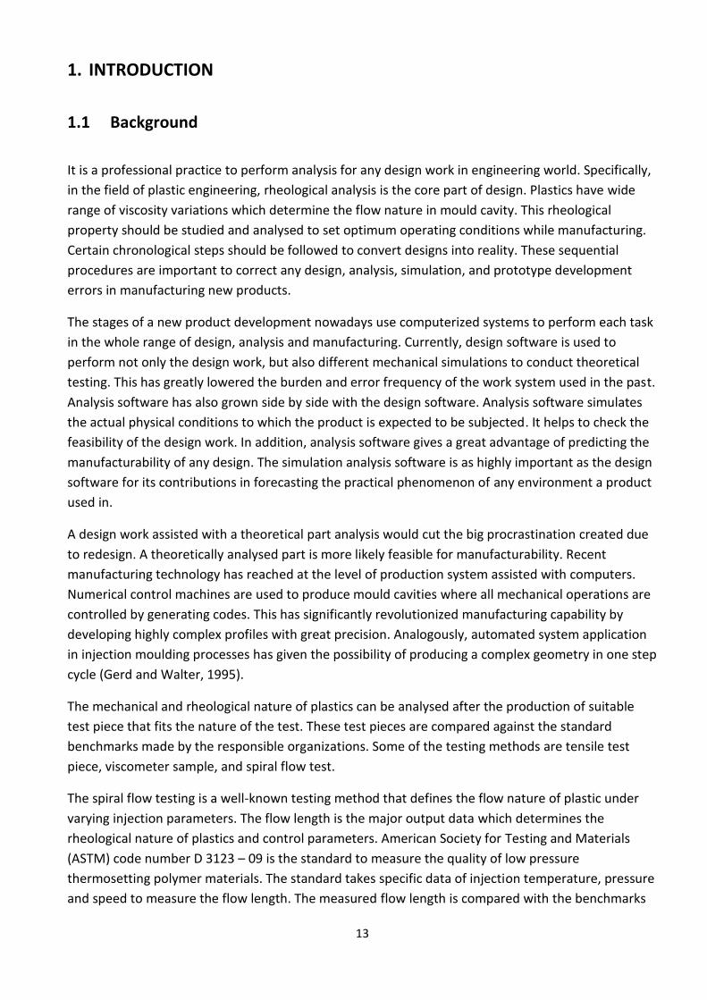
It is a professional practice to perform analysis for any design work in engineering world. Specifically,
in the field of plastic engineering, rheological analysis is the core part of design. Plastics have wide
range of viscosity variations which determine the flow nature in mould cavity. This rheological
property should be studied and analysed to set optimum operating conditions while manufacturing.
Certain chronological steps should be followed to convert designs into reality. These sequential
procedures are important to correct any design, analysis, simulation, and prototype development
errors in manufacturing new products.
The stages of a new product development nowadays use computerized systems to perform each task
in the whole range of design, analysis and manufacturing. Currently, design software is used to
perform not only the design work, but also different mechanical simulations to conduct theoretical
testing. This has greatly lowered the burden and error frequency of the work system used in the past.
Analysis software has also grown side by side with the design software. Analysis software simulates
the actual physical conditions to which the product is expected to be subjected. It helps to check the
feasibility of the design work. In addition, analysis software gives a great advantage of predicting the
manufacturability of any design. The simulation analysis software is as highly important as the design
software for its contributions in forecasting the practical phenomenon of any environment a product
used in.
A design work assisted with a theoretical part analysis would cut the big procrastination created due
to redesign. A theoretically analysed part is more likely feasible for manufacturability. Recent
manufacturing technology has reached at the level of production system assisted with computers.
Numerical control machines are used to produce mould cavities where all mechanical operations are
controlled by generating codes. This has significantly revolutionized manufacturing capability by
developing highly complex profiles with great precision. Analogously, automated system application
in injection moulding processes has given the possibility of producing a complex geometry in one step
cycle (Gerd and Walter, 1995).
The mechanical and rheological nature of plastics can be analysed after the production of suitable
test piece that fits the nature of the test. These test pieces are compared against the standard
benchmarks made by the responsible organizations. Some of the testing methods are tensile test
piece, viscometer sample, and spiral flow test.
The spiral flow testing is a well-known testing method that defines the flow nature of plastic under
varying injection parameters. The flow length is the major output data which determines the
rheological nature of plastics and control parameters. American Society for Testing and Materials
(ASTM) code number D 3123 – 09 is the standard to measure the quality of low pressure
thermosetting polymer materials. The standard takes specific data of injection temperature, pressure
and speed to measure the flow length. The measured flow length is compared with the benchmarks

14
for quality verification (ASTM, 2013). The thesis covers analogous analysis method for thermoplastic
materials. It studies all parameter variation influences on flow nature of thermoplastic polymers. As a
part of plastic engineering, the spiral flow testing experiment is quite important method to compare
the influences of different parameters in polymer processing. The spiral flow testing method can be
customized for any level of study in parametric variations; and this is one of them.
1.2 Objectives The major objectives of this thesis work are:
1. Design spiral test piece with constant radius increment of 12 mm
2. Design the spiral flow test piece mould on 156 * 156 mm2 standard mould plates
3. Perform a Moldflow simulation analysis on Autodesk Moldflow synergy software for low
density polyethylene (LDPE Luponen 1840 H) polymer
4. Perform Mastercam design and mill program for mould cavity and corresponding plates
5. Manufacture spiral test piece mould on CNC Haas milling machine based on part program
developed in Mastercam mill simulation
6. Develop theoretical rheological flow formula for semi-circular channel in isothermal
condition.
7. Manufacture spiral flow test piece on Engel CC 90 injection moulding machine for varying
operation settings.
8. Plot and compare injection pressure versus flow length graphs for theoretical findings,
Moldflow simulation and practical injection data
9. Calculate viscosity values for varying conditions of injection pressure and injection speed
alternatively
10. Plot injection pressure versus viscosity and injection speed versus viscosity graphs and
observe the parametric change influences on the viscosity nature
11. Calculate the power law index constant for LDPE Luponen 1840 H
12. Calibrate the injection pressure for LDPE Luponen 1840 H by plotting the injection
pressure versus flow ratio graph of the spiral test piece.
15
2. LITERATURE REVIEW
2.1 Injection moulding
2.1.1 Historical development of injection moulding
Injection moulding, as defined in injection moulding books, represents an important manufacturing
process in plastic part production (Gerd and Walter, 1995). Nowadays, the world has reached at a
time, where it is possible to produce complex plastic parts with injection moulding (Jack, 1998). It is
such prominent technology as it has made its remarkable importance in mass production. Aside from
the plastic injection moulding technology, there are contemporary plastic manufacturing
technologies which include; extrusions, blow moulding, thermoforming, transfer moulding and so on.
Among all these polymer processing technologies, the injection moulding takes a huge volume in
manufacturing plastic parts. Currently, it is impossible not to find an injection moulded plastic parts
that are used in humans’ day to day life.
There are different reports about the exact time injection moulding process has started. As it is noted
in Crawford (2005), quite significant innovation in the field was made in Germany, prior to the World
War II. The machine was very simple, manual and had a lower injection pressure that has only
allowed the production of small parts. The machine had a heated cylinder to melt plastic, and a
plunger to push the molten plastic into the mould. Levers were used to clamp the mould during the
process, and were the reason of having small pressure developed.
Subsequent developments in injection moulding machines were made after the first technology was
used; and eventually, the demands for the plastic products have risen continuously. The
developments of improved injection moulding machines have focused on the capacity of clamping
units and a wide option of versatility in production. Hence, the development of the next injection
moulding machine included the use of pneumatic cylinder that has lifted the burden off the
operators. It also and increased injection pressure. The major development in injection moulding
technology was introduced in late 1930, which employed the use of hydraulic system in injection
(Crawford 2005). This has revolutionized the injection system by accurately setting clamping force
during injection. Plastic deformations have been able to be reduced effectively due to this
technology. The production of different thermoplastic polymers had also risen side by side. During
these periods, the injection moulding machines have only been able to process certain specific
polymers. This has led to the need of designing and manufacturing injection moulding machines
which can incorporate the process of wide range of polymer types. Crawford (2005) explains that, in
1950 and onwards, the constant developments made in injection moulding machine manufacturing
have been successful in this regard. The basic design of injection moulding machines did not change
afterwards. In principle, every injection moulding machine follows certain mechanical procedure
during production.
Nowadays, many of developments in this technology focus in automating the control systems (Gerd
and Walter, 1995). The automation of a control system has made the technology of injection to be
highly sophisticated and self-controlling. Besides, the precision of part production, possibility of
manufacturing complex profile, high production rates and the ease with adjusting different
16
parameters for different types of thermoplastic polymers are the features of these newly mechanized
injection moulding machines.
2.1.2 Process of injection moulding
The process of injection moulding follows a sequential procedure during one cycle of operation in
producing a part. These processes are electromechanically controlled throughout the operation. The
injection moulding machines have different parts functioning integrated to perform the process
throughout. These parts are classified under sub categories called units, where a set of sub-
integrated operation performed to complete the whole process step by step. Generally, injection
moulding machines have the following components (Gerd and Walter, 1995).
Injection unit
Clamping unit
Tempering devices
Control systems
Sequential or co-operation of all the above components along with the central part of the process
which is the mould, results in a production of part. The first step in the process of injection is filling up
the plastic granules into the major carriage system of the injection machine, which is the hopper. The
raw material is prepared by proportional mixture of polymer granules and different additives. The
mass ratio mixture is made based on the physical and chemical property requirement on the finished
product. Granules are directly fed to the different zones of screw that reciprocates coaxially against a
hydraulically actuated cylinder (Menges, Michaeli and Mohren, 2000). The screw has feeding,
compression and metering zones on which these granules would change physically from their grain-
sized solid to a homogenized molten plastic ready for injection. The physical change of the granules
occurs procedurally. Right after the introduction from feed zone, they experience heat from the
cylinder barrel radially covering the screw. This cylinder has electrical heater bands which are the
primary start-up heat sources in melting polymers (Gerd and Walter 1995). The major polymer
melting process is due to a double side friction created among the barrel, granules and screw
threads. This friction helps in fast size reduction and building higher temperature in these granules.
When the granules are at the metering zone of the screw, it is expected that, the plastics are
physically homogenized and have a uniform temperature level throughout. After the completion of
plastic melt homogeneity, there should be enough shot size of molten plastic in front of the tip of the
screw. The clamping unit move transversely to close the mould before the injection. The clamping
unit could have a hydraulic cylinder or toggle lever to clamp moulds at parting lines. Clamping is a
very important step in injection moulding to protect molten plastic flash out occurring due to
misalignment and insufficient clamping system. After the mould halves are closed, molten plastic is
injected into the mould through the nozzle by the axial forward movement of the screw. The screw
pushes the molten plastic into the mould. After the mould cavity is filled with the molten plastic of
specified shot size, its temperature starts to drop by the cooling actions of tempering devices and
cooling channels. At this particular phase, compensation injection would be made for the volumetric
shrinkage caused due to the plastic solidification. Finally, after sufficient cooling, mould halves open
17
and the part is ejected. The cycle starts again following the same steps to produce the same type of
parts until the required amount is fulfilled.
2.1.3 Injection moulding machine
The injection machines nowadays are quite refined in their development and classified in many
regards. Classification of injection machines could be based on their clamping capacity, length,
injection capacity, and shot sizes. The clamping capacity of injection machines could be in a range of
5 tonnes up to 10,000 tonnes (Edward, 1994). Based on the need of injection machine from
laboratory purpose up until industrial manufacturing, the major classification of injection machines is
made based on their clamping force capacity in the ranges quoted above. An average injection
machine could have up to 300 tonnes of clamping capacity of which the equivalent SI unit value
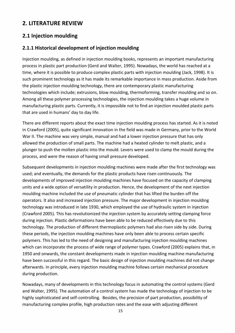
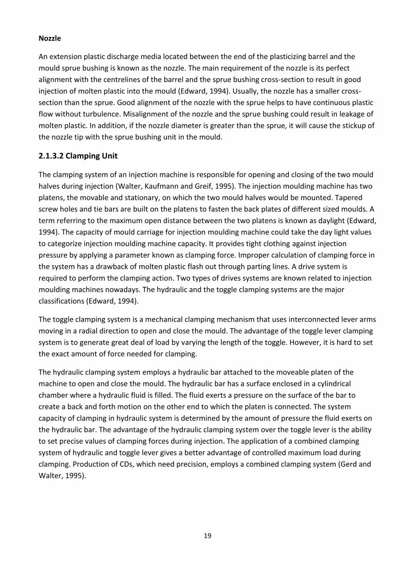
would be 3000 kN (Edward, 1994). The following schematic diagram presents the different units and
components of a general injection moulding machine.
Figure 1. Horizontal injection moulding machine layout diagram (ELITE, 2010)
Even if the control unit and the tempering systems are not included in the above diagram, the
complete injection moulding machine would include them for full functionality of the process. As it is
described earlier injection moulding process, injection moulding machines need to have the injection
unit, clamping unit, tempering devices and the control system. Each units and systems are studied in
the following sections.
2.1.3.1 Injection unit
The injection unit of an injection moulding machine is the first place where a polymer is introduced in
the injection moulding system. It starts with the feeding system (hopper) and ends with injection
nozzle through which molten plastic is injected into the mould. The injection unit mainly contains the
injection screw, barrel, heat control unit and the nozzle (Gerd and Walter, 1995). The polymer
material passes through the hopper up to the nozzle going through size reduction and state changes.
Pallets introduced into the feed section of the screw, would be transported by its rotating act. Most
of the heat in melting the plastic is generated from friction of these pallets against the barrel and
screw. The electric heater band mainly helps in providing a start-up thermal energy at the beginning
of the process. It also prevents the escaping of heat from the system by insulating the barrel radially.
18
Hopper
It is the simplest part of the injection unit having a funnel like shape to store raw materials right
before the process. The quality of a hopper is mainly based on how easily it can be operated, cleaned
and mounted. Modifications could be necessary while operating with hoppers; like stirrer to help
avoid stagnation while working with powder raw material (Gerd and Walter, 1995).
Screw
The central part of injection unit is the screw. It has three major sections. These are the feed,
compression and metering (Gerd and Walter 1995). The main function of the screw is to convey, melt
and homogenize the molten plastic. The three sections of the screw perform a step by step
integrated operation to have a homogenized uniform molten plastic. The feed section of the screw
transports the grain sized plastic granules to the compression section. It has a relatively larger flight
depth to maintain adequate flow rate of granules to the next compression section. In the
compression section, major size reductions occur as a result of friction and heat application from the
heat bands. At the end of this section, the plastic material is expected to melt completely. The last
section of the screw, the metering zone, helps to homogenize the molten plastic and maintain the
same temperature all throughout. The reciprocating motion of the screw helps to set the shot size of
the injection unit. The screw could be categorized based on its length to diameter (L/D) ratio, which
ranges mainly from 20:1 to 24:1; and its compression ratio (depth of flight in feed section to depth of
flight in metering section) ranging from 2.5:1 to 3:1 (Edward, 1994). In addition, depending on their
purpose, there would be a single stage or two stage injection screws (Edward, 1994). The two stage
screw has two compression and metering section to redo both compression and homogenizing to the
finest level by venting out water and monomer inclusions. However, most of the injection machines
have a universal thermoplastic screw where there is a single section of each of the feed, compression
and metering sections. Some very important terms related to screw are barrel capacity and residence
time. Both of them are interrelated machine data accessed from the machine provider. The residence
time is the amount of time a whole barrel full of polymer takes to be processed out (Edward, 1994). It
is quite important to determine the residence time to know whether a plastic spends too much time
in the barrel or not. This helps to protect the plastic from thermal degradation and a complete
change of physical property due to the lengthened time spent in barrel. Residence time is analysed
based on the standard general purpose polystyrene injection amount rated in ounces (oz).
Check Valve
The check valve is also known as non-return valve, found at tip of the metering section of the screw
to prevent the backflow of molten plastic during injection. The check valve has a sliding ring to slide
back and forth on a ring seat to open and close a cross-section during injection and metering
respectively. The backward sliding movement would place the sliding ring on the rear seat and shut
off the clearance between the barrel and top of screw to prevent back flow of polymer melt. The
inefficiency to properly function would cause visible impact on injection moulded product. The cavity
under fill, and material degrading due to the long-time stay in the barrel could be the result of
improper functionality of check valves (Gerd and Walter, 1995).
19
Nozzle
An extension plastic discharge media located between the end of the plasticizing barrel and the
mould sprue bushing is known as the nozzle. The main requirement of the nozzle is its perfect
alignment with the centrelines of the barrel and the sprue bushing cross-section to result in good
injection of molten plastic into the mould (Edward, 1994). Usually, the nozzle has a smaller cross-
section than the sprue. Good alignment of the nozzle with the sprue helps to have continuous plastic
flow without turbulence. Misalignment of the nozzle and the sprue bushing could result in leakage of
molten plastic. In addition, if the nozzle diameter is greater than the sprue, it will cause the stickup of
the nozzle tip with the sprue bushing unit in the mould.
2.1.3.2 Clamping Unit
The clamping system of an injection machine is responsible for opening and closing of the two mould
halves during injection (Walter, Kaufmann and Greif, 1995). The injection moulding machine has two
platens, the movable and stationary, on which the two mould halves would be mounted. Tapered
screw holes and tie bars are built on the platens to fasten the back plates of different sized moulds. A
term referring to the maximum open distance between the two platens is known as daylight (Edward,
1994). The capacity of mould carriage for injection moulding machine could take the day light values
to categorize injection moulding machine capacity. It provides tight clothing against injection
pressure by applying a parameter known as clamping force. Improper calculation of clamping force in
the system has a drawback of molten plastic flash out through parting lines. A drive system is
required to perform the clamping action. Two types of drives systems are known related to injection
moulding machines nowadays. The hydraulic and the toggle clamping systems are the major
classifications (Edward, 1994).
The toggle clamping system is a mechanical clamping mechanism that uses interconnected lever arms
moving in a radial direction to open and close the mould. The advantage of the toggle lever clamping
system is to generate great deal of load by varying the length of the toggle. However, it is hard to set
the exact amount of force needed for clamping.
The hydraulic clamping system employs a hydraulic bar attached to the moveable platen of the
machine to open and close the mould. The hydraulic bar has a surface enclosed in a cylindrical
chamber where a hydraulic fluid is filled. The fluid exerts a pressure on the surface of the bar to
create a back and forth motion on the other end to which the platen is connected. The system
capacity of clamping in hydraulic system is determined by the amount of pressure the fluid exerts on
the hydraulic bar. The advantage of the hydraulic clamping system over the toggle lever is the ability
to set precise values of clamping forces during injection. The application of a combined clamping
system of hydraulic and toggle lever gives a better advantage of controlled maximum load during
clamping. Production of CDs, which need precision, employs a combined clamping system (Gerd and
Walter, 1995).
20
2.1.3.3 Tempering device
Tempering device is a system of cooling in injection moulding process. The injected molten plastic
needs to cool down to a temperature level that solidifies the product in the cavity. This cooling
activity is performed by the tempering system of the injection moulding machine. Thermoplastic
polymers which demand lower mould temperature are usually cooled by the use of water in the
system. However, for polymers with higher mould temperature, oil should be used as a means of
tempering fluid. Theoretically, the cooling time is approximated as a function of wall thickness as
follows (Gerd and Walter, 1995).
( ) (1)
Where, , Cooling time (s)
And , Wall thickness (mm)
The tempering system of an injection moulding machine can be controlled to bring the temperature
of the product down to ejection temperature level. Most of the time, the tempering system is
assisted by external cooling system. Cooling system mainly uses water. The cooling system removes
the heat that occurs during molten plastic injection into the mould. The concept of heat transfer is
applied in developing external cooling system. These cooling systems are attached to the mould
plates in the injection systems. The role of the cooling system is to cool the molten plastic faster. The
cooling system in the injection moulding process is a very important part of the process when it
comes to industrial purpose. Due to the mass production system, cooling system affects rate of
production. The cooling time analysis with the above formula will get smaller with the application of
external cooling mechanism, which makes the overall cycle time to decrease for faster production
rate. Most of the time, the mechanism of cooling is done with water. Cooling channel holes with
specified diameters are drilled on moulding plates to circulate the water. Cooling channel patterns
could be either series or parallel (Gerd and Walter, 1995). Simple cooling system for small sized
products can have U shape or spiral channel depending on the part thickness and the need for
minimizing cooling time. The cooling channels are drilled with threaded holes up to certain depth
where the inlet outlet pipes should be tightened. The inlet pipes are attached to a water pipe through
hose, from which the cold water comes through and passes around the mould plates. After the
cooling is done with the cold water coming from the source, the warm water will be ejected through
the outlet pipe. The cooling system assists in fast cooling of molten plastic from its meting point
down to the mould temperature.
21
2.1.3.4 Control system
The control system of an injection moulding machine digitally controls all the mechanical actions
during the process. It controls the parameters of injection throughout the cycle of operation (Gerd
and Walter, 1995). The following lists of mechanical activities are controlled by the system;
The position and velocity of screw
Shot size of molten plastic
The holding pressure during injection
Mould closing and opening
Mould and barrel temperature
Hydraulic pressure
And, clamping force
The control system, not only controls the data fed to the machine, but also logically supervises the
sequence of operation. During plasticizing, the screw returns axially backwards to the reference
position. During this time, the machine closes the check valve; so that molten plastic will not leak out.
Before injection, the control system induces the action of closing the mould. Thermocouple sensor
transfers data to the control system to turn off heater bands if the temperature of the barrel is too
high, and turn on if the barrel temperature is too low. The control system also displays warnings of
too much cushion, if the reference position of the screw is too long. These logical controls are all
supervised by the control system to forward reasonable operation conditions.
In order to operate the process of injection, a person can choose setting up different figures for
different polymer types. The control system provides options to enter data on its platform. The
temperature control system gives option of adjusting temperature limits for mould and injection unit.
The pressure control system gives an option of setting up the amount of hydraulic pressure needed.
This hydraulic pressure is multiplied by an intensification ratio to calculate the corresponding
injection pressure level. Clamping force is also another parameter that determines the amount of
holding pressure multiplied by the projected area of the part. The clamping force can be set in kilo-
newton unit. Another important control system of injection is the position of screw versus injection
speed. This unit controls and plots the positions of screw against its speed at any position during the
cycle of injection. For optimum injection, the velocity of the screw can start with smaller velocity at
its reference position and goes up to 80% of maximum velocity at the midway and then slows down
at the end of the injection. The screw velocity can also stay constant during the position changes
made from reference up to the cushion start position. In this case, the graph of the screw velocity
versus screw position remains horizontal line.
22
Recent injection moulding machine innovations came up with digital display monitors to feed data
with key boards. Controlling is rather done with computerized system than switches. This gives an
automatic operation control system which helps to monitor the process while operating. The process
of injection moulding being controlled with microcomputers, not only helps to monitor the process,
but also gives an option of accessing and storing process data through printable formats (Gerd and
Walter, 1995). It also helps to exchange these process data with other working computers for further
data analysis.
2.2 Viscosity
The viscosity of polymers is a very important property in determining the rheological nature of
plastics. Viscosity data is the main input for mould and injection moulding machine designers in order
to accurately determine the process parameters. Viscosity is a dynamic property that changes with a
change in each parameters of injection moulding process. The main parameters that affect the
viscosity graphs are process temperature, pressure and injection speed (Dunkley, 1960). Along with
the parameters, the material chemical properties also play a role in varying the viscosity data of
plastics; the molecular weight and fillers are two of them. The main primary formula that governs the
viscosity in relation to the shear stress and shear rate is described as follows (Crawford, 2005, p.345).
(2.1)
Where, τ, Shear stress (Pa)
, Shear rate(s-1)
The shear rate is also defined in terms of the change in horizontal velocity and change in height
(Crawford, 2005).
(2.2)
Where, , Shear rate (s-1)
, Differential velocity (mm/s)
, Differential height (mm)
However, the expression in equation (2.1) gives a linear relationship which does not actually describe
the true shear viscosity nature of plastics. It gives a linear relationship of shear stress and shear rate,
which actually describes the nature of Newtonian fluid (Crawford, 2005). The graph of the shear
stress versus shear rate resembles a curve falling below the linear straight line with the increase in
shear stress. These polymers are called shear thinning fluids (Crawford, 2005). Engineers try different
approaches to quantitatively express the value of viscosity for polymers. However, the value of
viscosity does not keep constant even for the same polymer. Different parameter, especially the
temperature, affects the viscosity versus shear rate graph. With the increment of temperature, it is
observed that the values of viscosity have decreased for the same material at the same shear rate
values (Crawford, 2005). Hence, the different mathematical approach used to expresses the
23
rheological nature of plastics have errors to some extent; even if they are much better than leaving
the assumption of plastic to be Newtonian. These approaches are different with their focuses and
approximate value of mathematical expressions made on viscosity analysis. However, none of them
absolutely expressed the viscosity values perfectly; even if, they actually reduced errors made on
calculation of viscosity. These lists of approaches include the Power law, Carreau law and the law of
Vinogradow and Malkin (Crawford, 2005).
Newtonian fluids are expected to have certain ideal behaviours that would make them to have a
constant viscosity. This viscosity model helps to study the nature of fluid rheology at a basic level. In
addition, it is too much weak to precisely calculate the value of viscosity. Generally, the shear stress
divided by the shear rate gives a constant value for all values of temperature, pressure and injection
velocity variations. The fluids in this concept are considered to be highly incompressible, with steady
flow. This method is quite easy and straightforward to calculate despite of the less rigorousness.
The power law is another better approach to predict the rheological nature of fluids. It takes into
account the variation of shear rate along with the corresponding change in viscosity. The formula
below shows this relationship as implied (Crawford, 2005).
[
]
(2.3)
Where, , Required apparent viscosity (Pa.s)
, Reference viscosity (Pa.s)
, Apparent shear rate (s-1)
, Reference shear rate in (s-1)
, Power law index constant of a material
The power law is extensively used to explicitly figure out the inherent behaviour of shear viscosity. It
has a higher proximity to precision at higher shear rate values. However, at lower shear rates, the
power law lacks to accurately define the viscosity nature of actual fluids. Viscosity values at lower
shear rate are more closely considered like ideal fluids in power law. Besides, this law does not take
into account the temperature compensation variant. However, many of fluid analysis employ power
law to calculate the viscosity. The Viscosity variation can also be described as a function of shear
stress by rearranging the variables (Crawford, 2005).
[
]
(2.4)
Where, , Required apparent viscosity (Pa.s)
, Reference viscosity (Pa.s)
, Apparent shear stress (Pa)
, Reference shear stress (Pa)
24
, Power law index constant of a material
2.2.1 Power law index influence on shear stress versus shear rate graph
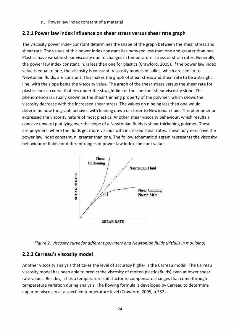
The viscosity power index constant determines the shape of the graph between the shear stress and
shear rate. The values of this power index constant lies between less than one and greater than one.
Plastics have variable shear viscosity due to changes in temperature, stress or strain rates. Generally,
the power law index constant, n, is less than one for plastics (Crawford, 2005). If the power law index
value is equal to one, the viscosity is constant. Viscosity models of solids, which are similar to
Newtonian fluids, are constant. This makes the graph of shear stress and shear rate to be a straight
line, with the slope being the viscosity value. The graph of the shear stress versus the shear rate for
plastics looks a curve that lies under the straight line of the constant shear viscosity slope. This
phenomenon is usually known as the shear thinning property of the polymer, which shows the
viscosity decrease with the increased shear stress. The values on n being less than one would
determine how the graph behaves with leaning down or closer to Newtonian fluid. This phenomenon
expressed the viscosity nature of most plastics. Another shear viscosity behaviour, which results a
concave upward plot lying over the slope of a Newtonian fluids is shear thickening polymer. These
are polymers, where the fluids get more viscous with increased shear rates. These polymers have the
power law index constant, n, greater than one. The follow schematic diagram represents the viscosity
behaviour of fluids for different ranges of power law index constant values.
Figure 2. Viscosity curve for different polymers and Newtonian fluids (Pitfalls in moulding)
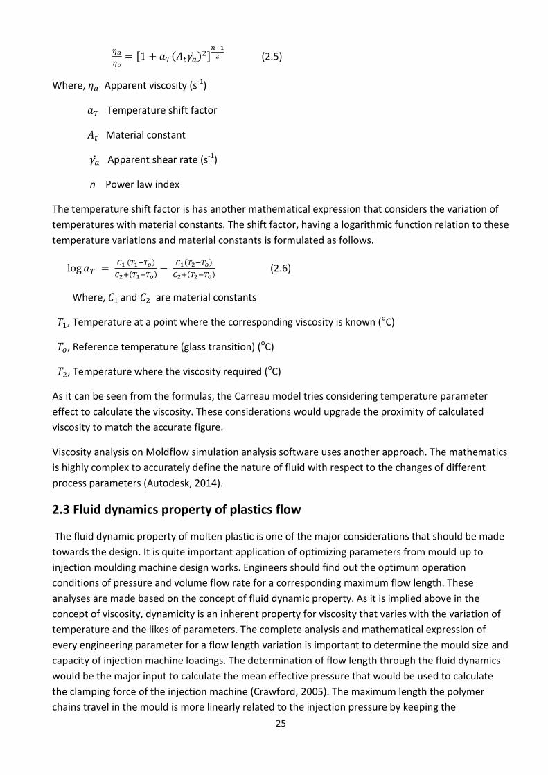
2.2.2 Carreau’s viscosity model
Another viscosity analysis that takes the level of accuracy higher is the Carreau model. The Carreau
viscosity model has been able to predict the viscosity of molten plastic (fluids) even at lower shear
rate values. Besides, it has a temperature shift factor to compensate changes that come through
temperature variation during analysis. The flowing formula is developed by Carreau to determine
apparent viscosity at a specified temperature level (Crawford, 2005, p.352).
25
[ ( )
]
(2.5)
Where, Apparent viscosity (s-1)
Temperature shift factor
Material constant
Apparent shear rate (s-1)
n Power law index
The temperature shift factor is has another mathematical expression that considers the variation of
temperatures with material constants. The shift factor, having a logarithmic function relation to these
temperature variations and material constants is formulated as follows.
( )
( )
( )
( ) (2.6)
Where, and are material constants
, Temperature at a point where the corresponding viscosity is known (oC)
, Reference temperature (glass transition) (oC)
, Temperature where the viscosity required (oC)
As it can be seen from the formulas, the Carreau model tries considering temperature parameter
effect to calculate the viscosity. These considerations would upgrade the proximity of calculated
viscosity to match the accurate figure.
Viscosity analysis on Moldflow simulation analysis software uses another approach. The mathematics
is highly complex to accurately define the nature of fluid with respect to the changes of different
process parameters (Autodesk, 2014).
2.3 Fluid dynamics property of plastics flow
The fluid dynamic property of molten plastic is one of the major considerations that should be made
towards the design. It is quite important application of optimizing parameters from mould up to
injection moulding machine design works. Engineers should find out the optimum operation
conditions of pressure and volume flow rate for a corresponding maximum flow length. These
analyses are made based on the concept of fluid dynamic property. As it is implied above in the
concept of viscosity, dynamicity is an inherent property for viscosity that varies with the variation of
temperature and the likes of parameters. The complete analysis and mathematical expression of
every engineering parameter for a flow length variation is important to determine the mould size and
capacity of injection machine loadings. The determination of flow length through the fluid dynamics
would be the major input to calculate the mean effective pressure that would be used to calculate
the clamping force of the injection machine (Crawford, 2005). The maximum length the polymer
chains travel in the mould is more linearly related to the injection pressure by keeping the
26
instantaneous temperature change constant. For these minor change in the temperature being
approximated as constant; the length of the polymer chains travelled determine how much pressure
an injection system should impart on the molten plastic. This pressure versus flow length relationship
determined from the fluid dynamics equation, would be used by mould designers to determine the
optimum pressure level used during injection into any kind of mould cavity.
The fluid dynamic analysis of these parametric relationships is based on the famous Hagen-Poiseuille
pressure loss formula (Crawford, 2005). The formula was first derived for Newtonian fluid where the
viscosity is kept constant. Hence, to determine the shear thinning or the plasticity natures, correction
factors of Rabinowitsch or power law index are used for the respective cases (Gerd and Walter,
1995). As of dealing with plastic, the focus is limited either with the ideal fluids or the correction is
made with power law to approximate in to the practical plastic nature. The Hagen-Poiseuille equation
is also used to determine the viscosity of plastics in capillary Viscometer. This also takes into account
the plastic to be incompressible in order to approximate the formula for ease of use. In addition, the
correction formula (power law) is used to approximately describe the viscosity nature. Hence, for
either of the objective the formula subjected to, it has proven its importance in parametric analysis.
The Hagen-Poiseuille formula takes into account the preliminary conditions of the fluid being;
incompressible
no slip between the fluid and wall (prefect shearing)
flow is steady, laminar and time independent
a constant viscosity The pressure drop in this formula is taken from the injection pressure that the injection machine
imparts from hydraulic system multiplied by intensification ratio (Crawford, 2005).
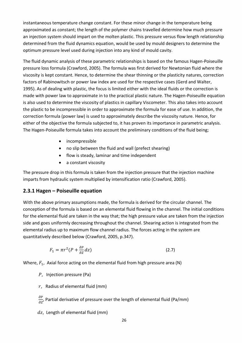
2.3.1 Hagen – Poiseuille equation
With the above primary assumptions made, the formula is derived for the circular channel. The
conception of the formula is based on an elemental fluid flowing in the channel. The initial conditions
for the elemental fluid are taken in the way that; the high pressure value are taken from the injection
side and goes uniformly decreasing throughout the channel. Shearing action is integrated from the
elemental radius up to maximum flow channel radius. The forces acting in the system are
quantitatively described below (Crawford, 2005, p.347).
(
) (2.7)
Where, , Axial force acting on the elemental fluid from high pressure area (N)
, Injection pressure (Pa)
, Radius of elemental fluid (mm)
, Partial derivative of pressure over the length of elemental fluid (Pa/mm)
, Length of elemental fluid (mm)
27
And the force that counteract to the high pressure force would be,
(2.8)
Where, , Axial force counteracting on the elemental fluid from low pressure area (N)
, Injection pressure (Pa)
, Radius of elemental fluid at any point in the flow channel (mm)
( ) (2.9)
Where, , Shear force due to the shearing action on the surface of the elemental fluid (N)
, Shear stress on the surface of the elemental fluid (Pa)
, Radius of elemental fluid (mm)
, Length of elemental fluid (mm)
The sum of three forces acting on elemental fluid due to pressure gradient and surface shear being
summed up to zero, would give the relationship between the shear stress and pressure gradient with
respect to flow length.
(2.10)
The expression for above justification looks like the following;
(2.11)
Another concept of expressing the shear force in terms of viscosity and shear rate from equation
(2.1),
But shear rate, as described in equation (2.2), is the change in velocity over the change in radius
putting the shear rate expression in terms of the change in velocity over radius in the shear stress
expression; and putting this expression in the first pressure over length expression, it would be
possible to interrelate the important parametric variables in one set of formula like the following.
(
)
Reshuffling the respective derivative to the same variables sides, and integrating radius from r up to R
and velocity from zero to maximum; the above expression would be finally turn into the following
formula (Crawford, 2005, 348)
28
(
)
(2.12)
Where, , Volume flow rate (mm3/s)
, Flow length (mm)
And analogously, the volume flow rate of a rectangular flow channel for isothermal flow condition is
formulated by the following equation (Crawford, 2005).
(2.13)
Where, H, Gap (thickness) between the flow channel (mm)
And T, Width (mm)
2.3.2 Pressure versus flow length property for plastics
The idea of comparison of flow length against injection pressure is quite important experiment that
determines optimum operation parameters. Different plastic injection factories and engineering
institutes conduct series of experiments on spiral flow length testing for optimization of parameters.
With injection speed and temperature held constant, the increase in pressure has resulted to
increase the flow length of thermoplastic polymers. The determination of flow length in a spiral flow
length testing method has a variety of engineering inputs that would give to injection moulding
machine and mould designers. The maximum loading capacity of injection machines takes these
pressure and flow length relationship data to determine the mean effective pressure that would be
applied while clamping the mould halves (Crawford, 2005).
Injection machine capacities, as referred above, are classified according to their clamping capacities.
These clamping capacities can be related with injection pressure. Performing a series of injection
pressure versus flow length experiment can determine the tonnage capacity needed for a specific
injection moulding process. The study of the relationship generally helps to find the optimum
operating conditions during polymer processing. The idea of this optimum operation condition is to
avoid any fault in injection process and find the best compromise of accelerated production process
to reduce manufacturing costs. Too fast injection with higher pressure would make products to have
air bubbles inside; as the air inside the mould cavity has less time to escape through vent holes.
Eventually the air would be trapped inside product which is a product quality defect. Besides, higher
injection pressure could force the molten plastic to flash through the parting lines; due to the less
clamping pressure. This results in a material waste. In the case of lower injection pressure, the
material is forced to stay in the moulding process for longer time with higher temperature. This effect
would make the material to lose its nature and degrade due to the thermal impact from heat bands
and friction.
The mould design analysis demands these relationships above all, to set theoretical parameters that
could match perfectly with the practical injection process. The mould design process, conceptually,
29
not only includes the part design, but also covers all engineering analysis to set optimum parameters
for manufacturing. As of the laboratory study conducted (TAPPI, 2014), the pressure versus flow
length data plotting showed a linear relationship. This data could be used for every mould design
process to validate the maximum flow length of the molten plastic in the mould and a corresponding
pressure level.
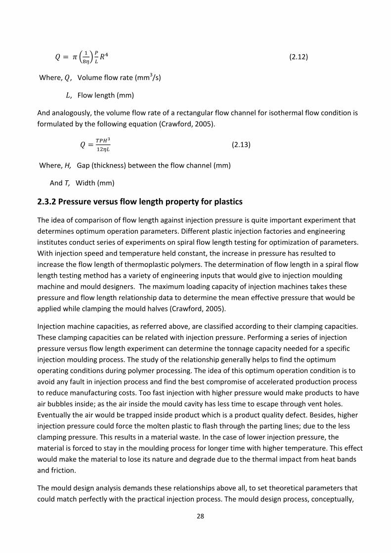
Another concept of injection process is clamping pressure which gives a clamping force when
multiplied by projected area of the part. The force is responsible for holding the two mould halves
together during the injection phase. This pressure is a function of flow ratio, which is the flow length
divided by wall thickness (Crawford, 2005). The following graph shows the relationship that holds
between the mean effective pressure and flow ratio for different polymers. This shows how the flow
length plays an important role in determining the clamping pressure for an injection pressure.
Figure 3. Mean effective pressure versus flow ratio for varying thickness of HDPE (Crawford, 2005)
Another important role of materials’ flow length during injection moulding process is its data input
for material quality determination. American Society for Testing and Materials (ASTM) has a standard
designation: D3123-09, for low pressure thermosetting materials quality verification. The standard is
practiced by setting parameters to specific figures. Under specific condition of pressure, temperature,
a melt flow index, and range of injection speed, the thermoset polymer is expected to have a flow
length that is a benchmark for verifying all other polymers during testing (American Society for
Materials and Testing, 2013). Even if ASTM does not have a designation for thermoplastic polymers,
analogues testing could be done to verify quality. The parameter that should be kept constant and
vary can be chosen on one’s interest. Apart from the pressure versus flow length relationship, it could
be taken as a study of injection speed versus flow length, or temperature versus flow length;
depending on nature of study and interest.
30
2.4 Archimedean spiral
Archimedes is one of the Greek philosophers, who is known for different scientific innovations (Texas
A&M University, 2014). The Archimedean spiral is one of them which has practical application in
locating corresponding points on a spiral path. The Archimedean spiral has a constant change of radii
between consecutive points on the spiral path and the relationship of the radius and angle is
governed by a basic formula given as follows (SquareCircleZ, 2013)
(2.13)
Where, , Radius at any point (mm)
, Start point of the curve (mm)
Constant of increment of the radius for each revolution
, Angle of revolution (radians)
If the spiral starts from the origin, then the above formula reduces to;
(2.14)
The major concept of the Archimedean spiral focuses on calculating out the circumference (length) of
the spiral. The practical application in science and technology is the finding of the path length of the
spiral. Finding out the path length of the Archimedean spiral helps to convert angular motions to
linear velocity for cam mechanisms in different mechanical assembly. It also helps to model rolls
made of paper or plastic of constant thickness wrapped round a cylinder. Any kind of profiles needed
to be made on moulds for the material testing based on standards also employ the concept of
Archimedean spiral for whichever change of radius over a revolution. The calculation of the spiral
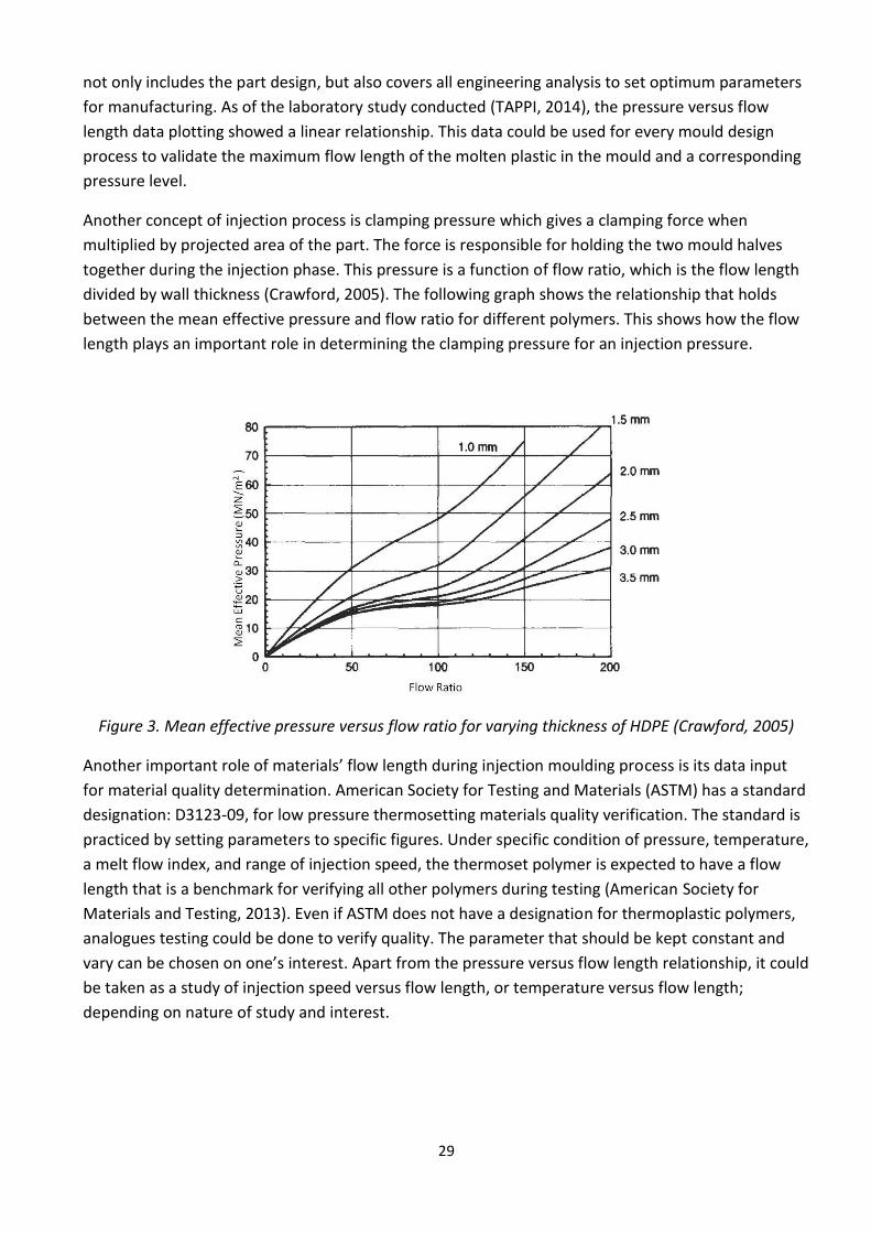
length needs a calculus concept to relate the change in radius over angle. The following picture
illustrates the fractional angle and radius relationship in terms of x and y decomposition to integrate
the total length for any required number of revolution (Wolfram Mathworld, 2013).
Figure 4. Derivation of the integral formula for arc length (Hubpages, 2014)
31
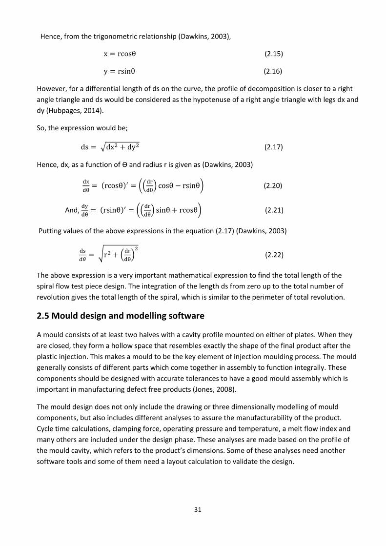
Hence, from the trigonometric relationship (Dawkins, 2003),
(2.15)
(2.16)
However, for a differential length of ds on the curve, the profile of decomposition is closer to a right
angle triangle and ds would be considered as the hypotenuse of a right angle triangle with legs dx and
dy (Hubpages, 2014).
So, the expression would be;
√ (2.17)
Hence, dx, as a function of ϴ and radius r is given as (Dawkins, 2003)
( ) ((
) ) (2.20)
And,
( ) ((
) ) (2.21)
Putting values of the above expressions in the equation (2.17) (Dawkins, 2003)
√ (
)
(2.22)
The above expression is a very important mathematical expression to find the total length of the
spiral flow test piece design. The integration of the length ds from zero up to the total number of
revolution gives the total length of the spiral, which is similar to the perimeter of total revolution.
2.5 Mould design and modelling software
A mould consists of at least two halves with a cavity profile mounted on either of plates. When they
are closed, they form a hollow space that resembles exactly the shape of the final product after the
plastic injection. This makes a mould to be the key element of injection moulding process. The mould
generally consists of different parts which come together in assembly to function integrally. These
components should be designed with accurate tolerances to have a good mould assembly which is
important in manufacturing defect free products (Jones, 2008).
The mould design does not only include the drawing or three dimensionally modelling of mould
components, but also includes different analyses to assure the manufacturability of the product.
Cycle time calculations, clamping force, operating pressure and temperature, a melt flow index and
many others are included under the design phase. These analyses are made based on the profile of
the mould cavity, which refers to the product’s dimensions. Some of these analyses need another
software tools and some of them need a layout calculation to validate the design.
32
During early ages, engineers were supposed to draw every pieces of mould component on A0 sized
papers and transfer the design to a tracing paper for a blue print. Designs were made by hand with
the help of drawing equipment. These were tedious, time taking and too much prone to errors.
One of the most important design developments is the introduction of design software that
revolutionized the world of engineering. AutoCAD, officially successful software that has been used
for multi-purpose design for decades, is still the primary choice for most of design purpose around
the world (Autodesk Moldflow Insight, 2009).
The innovation of new software has ever been easing up the loads of engineering designs by saving
time and increasing accuracy. Currently, Solid Edge, SolidWorks, Parasolid and many other software
types are developed that have many modification tools. This has eased up the work of design even
more accurate by modelling and simulation. SolidWorks and Solid Edge have especially Add-in tools
which give capabilities to perform a multi-engineering analysis, like mould tooling and flow
simulations. The two dimensional drawing, three dimensional modelling, surface modification
capabilities have removed every procrastinations in design works. Modelling software gives the
possibility for users to easily design through its perfect user friendly interface and interactive nature.
In the case of mould design, the mould tooling Add-in software has multiple standard plates from
which, a user can choose. This is a very important design procedure as long as every design needs
standards. Hasco is one of most resourced standard for most of mould designs. It incorporates from
the smallest plate sizes of 96 mm * 96 mm up to 256 mm * 256 mm, with a K- series designation.
Each plate in a specific mould set has a K name for its designation (HASCO, 2014). The core and cavity
are the main components of the mould set. Hence, there are varieties in thickness of cavity and core
plates for the same dimension of standard plate sizes to incorporate manufacturing of different
products with different depths. Standards are quite important in design as long as designs are made
based on the agreed dimensions and designations all over the world. The Solid Edge software has
every Hasco standard plates in its library for the user to access in mould tooling. Hence, for most of
the cases, the modelling software simulates mould assembly and analyse mechanical properties of
the plates. With every design and assembly made on this software, and checked for perfect
alignment of parting line, there will not be any error in manufacturing. The simulation of mould
assembly helps to visualize what would actually happen after the production of the mould plates with
accurate tolerances. Hence, the design software has moved one step more to make design works so
simple and error free (SIMENS, 2014).
2.6 AutoCAD Moldflow simulation theories and analysis
As the innovation towards modelling software helps a great deal of design possibilities, the Moldflow
simulation analysis software also plays a great role in predicting the injection of plastic in to the
machine virtually. It simulates products in injection process at the design stage that saves a lot of
energy and cost before the actual mould is produced and loaded on injection machine. Moldflow
simulation actually gives credible technical information in the injection process. All of the control
mechanisms and process settings are included to represent the actual injection moulding machine
process. It is such powerful software that analyses data of customized settings by implementing
33
digital prototype technology before ideas come to reality in manufacturing sector. Mechanical,
thermal and rheological properties are completely included in the raw material settings. In fact,
Moldflow analysis from Autodesk has the largest raw material and machine varieties in the world.
The Moldflow simulation analysis follows simple ways which are quite technical and match the looks
of control setup in injection moulding machines. It goes on analysing to give an optimum ways of
manufacturing (Autodesk Moldflow communicator, 2012).
The Moldflow analysis starts with importing and meshing the product. It gives an option for the user
to import files from different modelling software and mesh the product in tetrahedral. Three types of
mesh options are incorporated. 3D mesh is for plastic materials with thicker walls. However, dual and
mid-plane meshes are for thin plastic parts. Thermoplastics and thermosetting plastics have the
possibility to be analysed in this software. Following the mesh completions, the Moldflow software
gives the option for user to choose material. As quoted earlier, the Moldflow simulation analysis
software from Autodesk includes all material properties to be studied during injection. The thermal,
mechanical and rheological data are at most predicted to perfectly match the actual materials in real
world injection (Autodesk Moldflow Insight, 2009).
One of the most important properties is the materials’ viscosity nature; of which dynamism is an
inherent property. The Moldflow synergy software predicts the viscosity data with varying models.
These models are dependent upon the projections of product design, cooling system and operating
conditions. Matrix, Cross-WLF (Williams-Landel-Ferry) and Second Order are the viscosity models
used for thermoplastics. Each of these viscosity models have their interests depending on temperate,
pressure and shear rates. The Cross-WLF model describes the viscosity dependence, over shear rate,
temperature and pressure variations. The Matrix model uses measured values of pressure
temperature and shear rate values to determine the apparent viscosity. The third model, Second
order, uses the temperature and shear rate viscosity dependency. The Cross-WLF and Second order
viscosity models use the materials’ constants (data – fitted constants) along with predetermined
values of temperature and shear rate to calculate the viscosity at a required point. The formulas for
these two viscosity models are reasonably compared with Power law and Carreau’s model. The
models take into account every variation in viscosity as a result of the changes in temperature and
shear rate. Besides, they are able to predict viscosity behaviour at lower shear rate values (Autodesk,
2014).
As it is described earlier, the Cross-WLF viscosity model defines viscosity models by relating pressure,
temperature and shear rate. The viscosity versus shear rate graph is plotted based on the following
formula relating the variables at different levels (Autodesk, 2014).
(2.23)
34
Where:
, Melt viscosity (Pa.s) , Zero shear viscosity or the 'Newtonian limit' in which the viscosity approaches a constant
at very low shear rates(Pa.s)
, Shear rate (s-1) , Critical stress level at the transition to shear thinning, determined by curve fitting (Pa) , Power law index in the high shear rate regime, determined by curve fitting.
The viscosity with the corresponding shear rate is determined through the above formula for any operation condition during injection. The simulation software also interpolates the viscosity versus shear rate graph during the whole range of fill times.
It also takes analogous technique to calculate, model and plot the graph of viscosity Second order viscosity model. However, this time, only the shear rate and temperature dependencies are reflected. It takes different data-fitted constants and relating temperature values into a form that ultimately describe the viscosity nature. Viscosity graphs are plotted based on the following formula (Autodesk, 2014).
(2.24)
Where:
, Viscosity (Pa.s)
, Shear rate (s-1) , Temperature (oC). And to are data-fitted coefficients
The Autodesk Moldflow analysis software, after meshing a product it gives a user to choose the fill option. The fill options can be fill, fill and pack, and fill and pack and cool. It also depends on the type of product one would like to analysis. Fill option, as its name implies, only fill the design with the molten plastic. The fill and pack option provides the possibility to fill and pack and fill more plastic to compensate the shrinkage. The third option is the fill, pack and cool. It setup a cooling system to control the cycle time. The cooling option gives the opportunity to cool the injected plastic faster, if a normal filling takes longer time to cool due to the wall thickness of the product (Autodesk Moldflow Insight, 2009).
The next and major part of the simulation which is quite important is the process control. The controls are classified into material, injection machine and process control. The material control has lists of all thermoplastic and thermosetting material libraries a user can choose from. Autodesk Moldflow synergy has the world’s largest material database with their manufacturer and trade name lists. The process control is the key part a user can use to match the virtual injection looking similar to the actual injection process controls. This helps engineers to figure out design and manufacturing errors. The process control can be performed with a fill and velocity/pressure switchover control options. The fill control options are injection time and volume flow rate. The user can set either of the parameters to control the fill options. The velocity/pressure switchover control options gives a control possibility with injection pressure and ram speed versus ram position control options. A user can either control the switchover control option by setting injection pressure value, or set data values for ram speed versus ram position. The data entered for ram speed and ram position are linearly
35
related to control the injection speed. As the screw moves forward to inject the molten plastic into the cavity, the position of the screw tip with its velocity is plotted automatically by the software for control options. Another way of controlling the process is the mould machine type. A user can choose the type of injection machine that could potentially match the practical injection process. Majority of classification for these machine types are based on clamping capacity and screw diameter. Finally, a user can also set a mould material due to the thermal conductivity and expansion phenomenon. Tool steel types are identified based on standards and set in this control option for a user to choose from (Autodesk Moldflow Communicator, 2012).
2.7 Mastercam simulation and HAAS Mill
CNC software, inc. is one of the oldest developers of CAD/CAM, which is computer based software. The CNC software, inc. is also the first company to introduce design and machining integrated on software. The Mastercam software is used to help the virtual development of parts on a computer and also used to guide computer numerical control (CNC) machine tools to practically develop the part. The Mastercam software is basically designed for both engineers and machinists by integrating both design and machine operations. Geometry creation is the first thing to do while using Mastercam (CNC software, inc., 2000).
Kelly and Jon (2002) described in their Mastercam practical training manual that, it is possible to create geometries on one of the three application areas. Mastercam has these three application areas used to produce a geometry based on the type of machining required. These application areas are Mastercam design, Mastercam milling and Mastercam lathe. A set of predefined toolpaths are set to help out the machining process on CNC after the geometry creation. Some of the terms related with Mastercam are defined below;
Contour toolpath - CNC software, Inc. (2000) guide defines a contour toolpath as the operation that removes material along a cutter path defined by a curve or chain of curves. The contour toolpath follows a closed or open geometry made to remove part while machining.
Drilling - the Mastercam drill toolpath performs both the centre drill and drilling holes of different diameters on a work piece.
Pocketing – Kelly and Jon (2002) define pocketing as a module used to create toolpaths to remove material in a closed contour or to face mill the top of a part. Pocketing toolpath helps to perform milling operation on a closed geometry of a working stock.
James Madison (1996) defined in his CNC machining handbook that, a computer numerical control is
a computer assisted process to control general purpose machines through instructions generated by
a processor stored in memory system or storage media. These controllers are numerical units which
are series of numbers making the numerical commands work on controlling.
Modern CNC milling machines usually consists of table that moves in y-direction and a chuck moving
in X-Z direction. These combined movements would help to machining a work piece on any position
of X-Y-Z coordinate. The machine has its origin (X 0.000, Y 0.000, Z 0.000) where all the operations
would start from. Hence, location with respect to the origin should be made for every points where
machining is to be made (Haas Factory Outlet, 2013).

36
CNC milling machines have system of elements which integrate during a whole cycle of operation
(Institute for machine tools technology, 2010). These elements are;
Part program
Program input device
Machine control unit
Drive system
Machine tool
And feedback system
A synchronized operation of these systems helps the CNC machines to perform any kind of machining
practically.
A part program consists of a series of codes that describes how a specific design produced on
CAD/CAM can actually be produced on the CNC machine. These codes are usually written with G and
M along with numbers proceeded. The codes are series of letters and numbers that describe specific
movements of the tool to produce parts (Denford). The part program generally consists of all
geometrical movements of the tools from the start up to the end of part production. This part
program can be broken down to a set of aggregate codes of words with each of them are
combination of letters and numbers. These words refer a specific cutting operation or movement of
tool. The program letters starting with G and M are recognized by the CNC machine control unit. A
set of simulation developed on CAD/CAM can be loaded to the CNC machine’s computer which can
be simulated directly or edited through its control unit. The machine controller detects and interprets
the program and sends a signal of sequence of operation to the machine elements.
The program input devices are parts which help the part program to be entered into the machine.
Keyboard, punched tape readers, diskette could be one of them which use a network serial port to
load the program.
The machine control unit is the most important system of CNC machines. It performs the whole range
of activities starting from decoding the part program codes, up to implementing and amplification of
interpolations for any kind of linear, circular and helical movements of the axis during the operation
(Virginia Tech, 2000). It also receives feedback on the position and speed for each drive axis. This
helps the CNC to accurately define the feed rate of the tool during operation and locate the offset
position before the next operation.
The drive system actually refers to the servomotor in CNC. The interpolation developed in the
machine control unit would be amplified through this drive system. Hence, any physical movement of
the table would be possible depending on the coordinate given.
The machine tools are any of the installed tools necessary to perform any machining operations on
the CNC. The machine control takes a reference between the position of the table axis and the
spindle to determine the tool movements. It also takes a Z-offset value for each installed tools
measuring the gap between the surface of the table and the tool tip.

37
Finally, the feedback system always uses the speed and position transducers to determine the feed
and position of the tool at any time. It sends these data to the machine control unit. The machine
control unit takes the feedback and compares against the reference signals to correct the feed and
speed errors.
38
3. METHOD
The lists of methods that are used to analyse the different results needed to be observed are dealt in
detail in this part of the thesis. The methods used in this thesis are chronologically linked to assess
the parametric relationship of differ variables. These methods are classified into three. The first
method is the Archimedean spiral length calculation; the second one is the isothermal flow analysis
through the semi-circular channel. The last one is the calculation of the power law index for LDPE
Luponen 1840 H polymer to observe the influence of the polymer’s non-Newtonian nature. The
method bases the power law index analysis formula. The step by step formula derivation is done for
analysing these different parametric variables based on the initials or analogues analysis made for
different flow patterns. Finally, all types of relevant analysis and comparison are made in this section
based on the engineering findings on the first three methods of this section.
3.1 Archimedean spiral length analysis method
The Archimedean spiral is the basic principle used in this thesis to determine the length of the spiral
flow channel produced on the cavity plate of the mould set. The initial concept of derivative is taken
in this thesis to formulate and calculate the simulation and practical injection. The initial concept that
defines the Archimedean spiral relates the change of radius through the differential change of angle
of revolution. Hence, from equation (2.14)
However, the standard spiral mould design in this thesis has an increment of 12 mm in radius for
each revolution of the spiral. Putting this relationship in the above formula, the method determines
the constant of increment, b. Hence,
b = 1, 91 mm
For any arbitrary position on the spiral path, the relationship between the angle of revolution and the
radius is expressed as;
(3.1)
The above linear relationship between the radius and angle of revolution is a major input to integrate
and find out the length of spiral for any number of revolutions. Hence, taking the differential spiral
length formula from equation (2.22) and putting the radius and angle relationship, the method
integrate for spiral length,
Hence,
√ (
)
Putting r in terms of ϴ,
√(( ) ( ) (
)
)
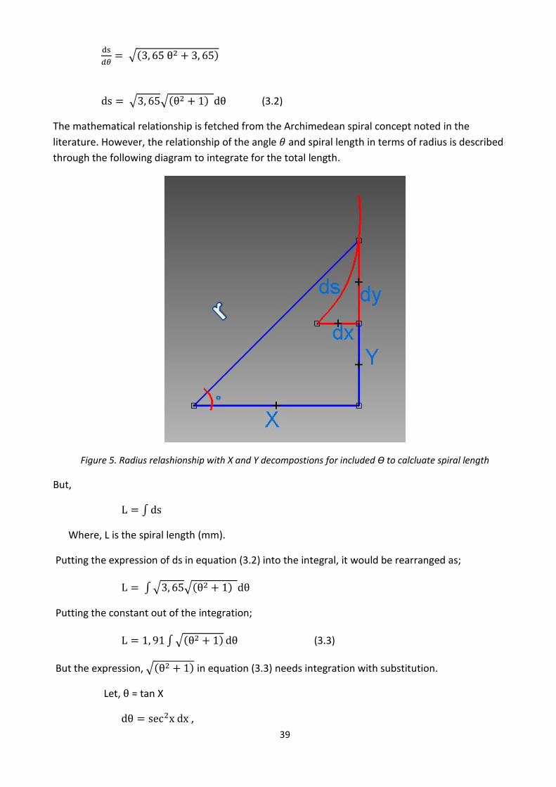
39
√( )
√ √( ) (3.2)
The mathematical relationship is fetched from the Archimedean spiral concept noted in the
literature. However, the relationship of the angle and spiral length in terms of radius is described
through the following diagram to integrate for the total length.
Figure 5. Radius relashionship with X and Y decompostions for included ϴ to calcluate spiral length
But,
∫
Where, L is the spiral length (mm).
Putting the expression of ds in equation (3.2) into the integral, it would be rearranged as;
∫√ √( )
Putting the constant out of the integration;
∫√( ) (3.3)
But the expression, √( ) in equation (3.3) needs integration with substitution.
Let, = tan X
,
40
Hence, the expression in equation (3.3) would be
∫ (3.4)
Using integration by parts rule once again for the above equation (3.4)
∫ ∫
Let,
And,
So, putting the above expression of parts, and taking the coefficient 1, 19 away for convenience,
∫ ∫
∫ ∫
∫ ∫( )
∫ ∫( )
∫ ∫ (3.5)
But, ∫ ( )
Putting the above expression in equation (3.5)
∫ ( )
So,
∫ ( ( )) (3.6)
From trigonometric relation,
If , then,
√ ,
Putting back the expression in terms of in equation (3.6) and replacing it in equation (3.4) an
expression for the length of the spiral being explicitly formulated as follows,
( √ ) ( √ )
(3.7)
Finally, taking back the coefficient value of 1, 91 in the above equation (3.7), the Archimedean spiral
length calculation made in this thesis; that has a constant 12 mm increment in radius for every
revolution is described as follows.
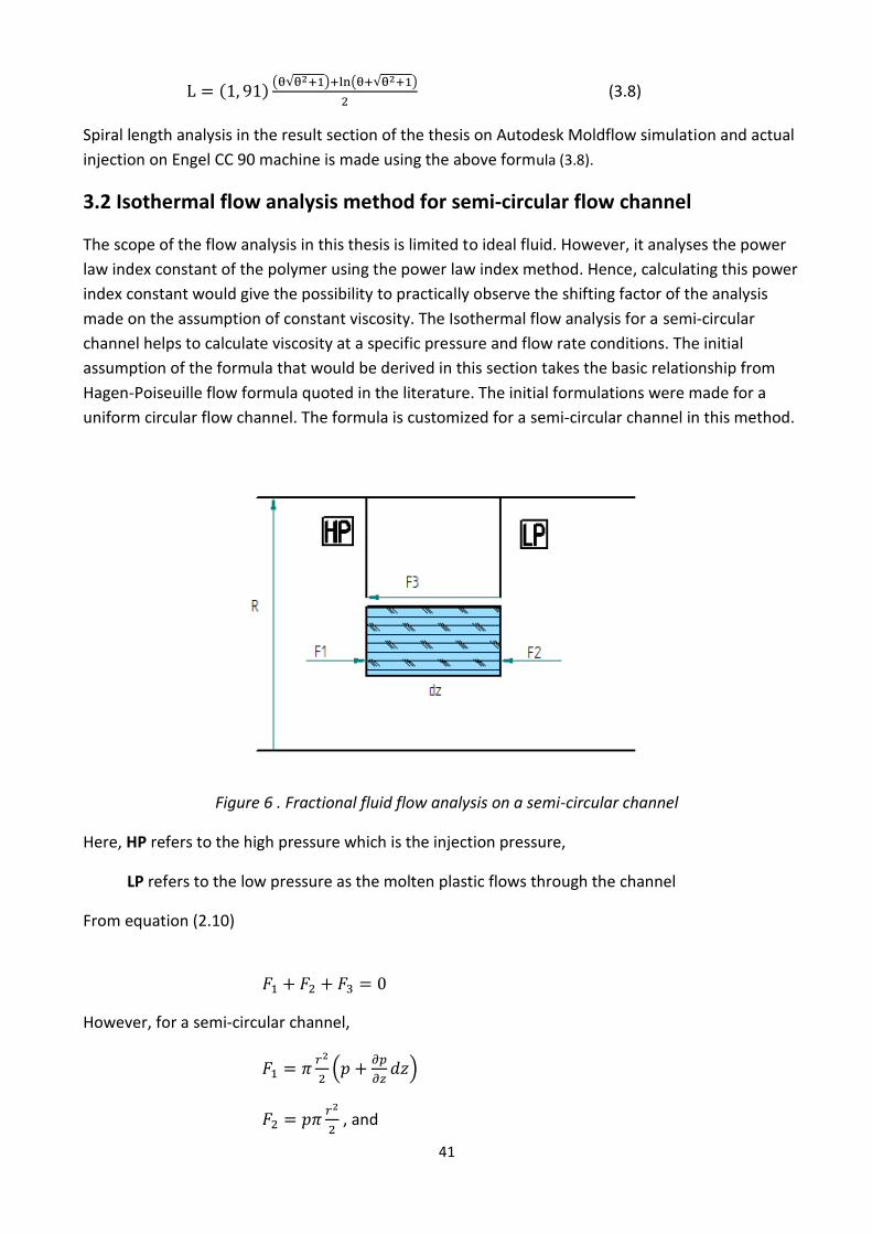
41
( )( √ ) ( √ )
(3.8)
Spiral length analysis in the result section of the thesis on Autodesk Moldflow simulation and actual
injection on Engel CC 90 machine is made using the above formula (3.8).
3.2 Isothermal flow analysis method for semi-circular flow channel
The scope of the flow analysis in this thesis is limited to ideal fluid. However, it analyses the power
law index constant of the polymer using the power law index method. Hence, calculating this power
index constant would give the possibility to practically observe the shifting factor of the analysis
made on the assumption of constant viscosity. The Isothermal flow analysis for a semi-circular
channel helps to calculate viscosity at a specific pressure and flow rate conditions. The initial
assumption of the formula that would be derived in this section takes the basic relationship from
Hagen-Poiseuille flow formula quoted in the literature. The initial formulations were made for a
uniform circular flow channel. The formula is customized for a semi-circular channel in this method.
Figure 6 . Fractional fluid flow analysis on a semi-circular channel
Here, HP refers to the high pressure which is the injection pressure,
LP refers to the low pressure as the molten plastic flows through the channel
From equation (2.10)
However, for a semi-circular channel,
(
)
, and
42
( )
Summing the expressions of forces to zero,
(
)
( )
( ( ) )
( ( ))
( )(
) (3.9)
Another expression of shear stress from the rheological point of view defines fluid in equation (2.1)
as,
But the shear rate is also defined in equation (2.2) as the change of fluid velocity over the change of
radius,
Combining the above two equations,
Now, putting the above shear rate expression in the pressure formula and equating with equation
(3.9) would give the major formula needed in this method part of the thesis to calculate viscosity,
( )(
)
(
) (
)
( ) (3.10)
Hence, integrating the above equation (3.10) for the two variables of velocity and radius where the
range of radius being from r up to R,
∫ ∫ (
)
(
)
( )
∫
(
( ))∫
(
) (
) (
( )) ( ) (3.11)
The velocity through the semi-circular channel is defined by the above formula. The initial velocity
occurs when the small radius is zero; r = 0
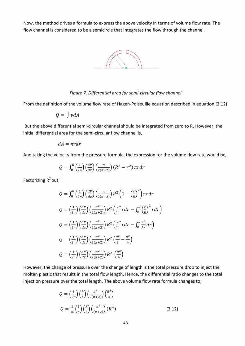
43
Now, the method drives a formula to express the above velocity in terms of volume flow rate. The
flow channel is considered to be a semicircle that integrates the flow through the channel.
Figure 7. Differential area for semi-circular flow channel
From the definition of the volume flow rate of Hagen-Poiseuille equation described in equation (2.12)
∫
But the above differential semi-circular channel should be integrated from zero to R. However, the
initial differential area for the semi-circular flow channel is,
And taking the velocity from the pressure formula, the expression for the volume flow rate would be,
∫ (
) (
) (
( )) ( )
Factorizing R2 out,
∫ (
) (
) (
( )) ( (
)
)
(
) (
) (
( )) (∫
∫ (
)
)
(
) (
) (
( )) (∫
∫
)
(
) (
) (
( )) (
)
(
) (
) (
( )) (
)
However, the change of pressure over the change of length is the total pressure drop to inject the
molten plastic that results in the total flow length. Hence, the differential ratio changes to the total
injection pressure over the total length. The above volume flow rate formula changes to;
(
) (
) (
( )) (
)
(
) (
) (
( )) ( ) (3.12)
44
3.3 Power index law method
The thesis has a scope of analysing the plastic melt flow by taking the concept of Newtonian fluid
flow with isothermal conditions. However, it is known that plastics behave far differently from the
ideal fluids. The thesis analyses the shifting factor of this difference by calculating the power law
index at a 220 0C temperature for specific low density polyethylene with a commercial name of
Luponen 1840 H. The calculation of the power law index constant explains best the rheological
behaviour of the specified polymer at assumed temperature level. The influence of the power law
index constant can be seen on the graph plots of viscosity against injection speed. The method uses
the formula from the power law relating apparent and reference viscosity and shear stress values.
The actual spiral products produced on two different injection pressure and injection speed levels are
taken to calculate the power law index of the polymer using the following power law formula from
equations (2.3) and (2.4).
[
]
3.4 Mould design method
The mould design method used in this thesis is a three dimensional modelling software known as
Solid Edge. The design method also uses another analogues modelling software known as SolidWorks
to give an option of design accessibility. Besides, the mould design follows the Hasco standard plates
for modelling the mould set. The design method includes the design of the product (spiral) and the
mould set. For the case of the mould set, the method presents all the plate names and specifications
based on the standards represented in Hasco. The following table presents all the design contents of
specification for each plate. Design works follow the plate standards listed below.
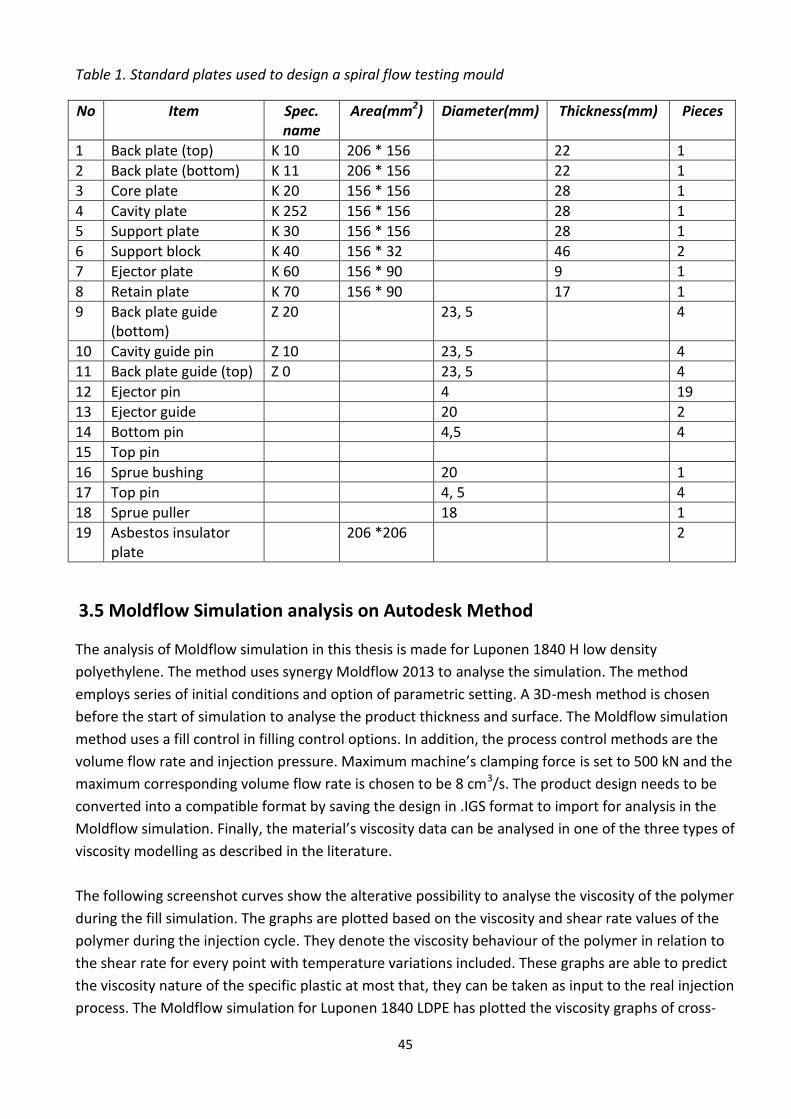
45
Table 1. Standard plates used to design a spiral flow testing mould
No Item Spec. name
Area(mm2) Diameter(mm) Thickness(mm) Pieces
1 Back plate (top) K 10 206 * 156 22 1
2 Back plate (bottom) K 11 206 * 156 22 1
3 Core plate K 20 156 * 156 28 1
4 Cavity plate K 252 156 * 156 28 1
5 Support plate K 30 156 * 156 28 1
6 Support block K 40 156 * 32 46 2
7 Ejector plate K 60 156 * 90 9 1
8 Retain plate K 70 156 * 90 17 1
9 Back plate guide (bottom)
Z 20 23, 5 4
10 Cavity guide pin Z 10 23, 5 4
11 Back plate guide (top) Z 0 23, 5 4
12 Ejector pin 4 19
13 Ejector guide 20 2
14 Bottom pin 4,5 4
15 Top pin
16 Sprue bushing 20 1
17 Top pin 4, 5 4
18 Sprue puller 18 1
19 Asbestos insulator plate
206 *206 2
3.5 Moldflow Simulation analysis on Autodesk Method
The analysis of Moldflow simulation in this thesis is made for Luponen 1840 H low density
polyethylene. The method uses synergy Moldflow 2013 to analyse the simulation. The method
employs series of initial conditions and option of parametric setting. A 3D-mesh method is chosen
before the start of simulation to analyse the product thickness and surface. The Moldflow simulation
method uses a fill control in filling control options. In addition, the process control methods are the
volume flow rate and injection pressure. Maximum machine’s clamping force is set to 500 kN and the
maximum corresponding volume flow rate is chosen to be 8 cm3/s. The product design needs to be
converted into a compatible format by saving the design in .IGS format to import for analysis in the
Moldflow simulation. Finally, the material’s viscosity data can be analysed in one of the three types of
viscosity modelling as described in the literature.
The following screenshot curves show the alterative possibility to analyse the viscosity of the polymer
during the fill simulation. The graphs are plotted based on the viscosity and shear rate values of the
polymer during the injection cycle. They denote the viscosity behaviour of the polymer in relation to
the shear rate for every point with temperature variations included. These graphs are able to predict
the viscosity nature of the specific plastic at most that, they can be taken as input to the real injection
process. The Moldflow simulation for Luponen 1840 LDPE has plotted the viscosity graphs of cross-
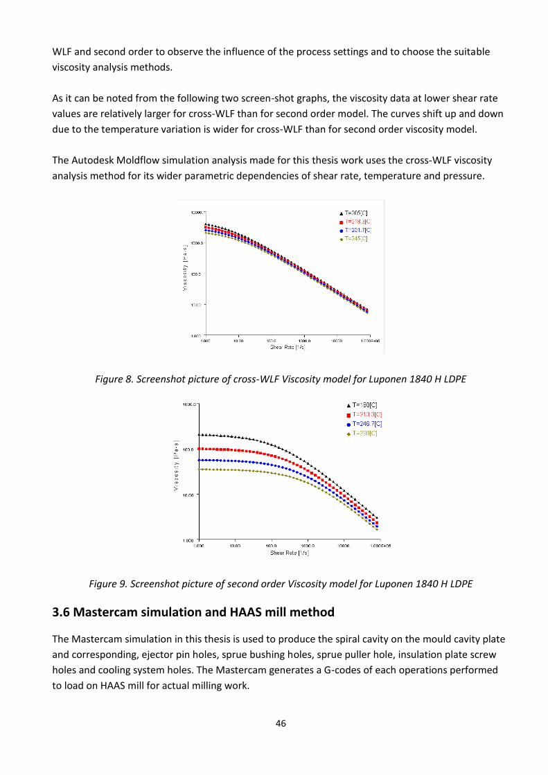
46
WLF and second order to observe the influence of the process settings and to choose the suitable
viscosity analysis methods.
As it can be noted from the following two screen-shot graphs, the viscosity data at lower shear rate
values are relatively larger for cross-WLF than for second order model. The curves shift up and down
due to the temperature variation is wider for cross-WLF than for second order viscosity model.
The Autodesk Moldflow simulation analysis made for this thesis work uses the cross-WLF viscosity
analysis method for its wider parametric dependencies of shear rate, temperature and pressure.
Figure 8. Screenshot picture of cross-WLF Viscosity model for Luponen 1840 H LDPE
Figure 9. Screenshot picture of second order Viscosity model for Luponen 1840 H LDPE
3.6 Mastercam simulation and HAAS mill method
The Mastercam simulation in this thesis is used to produce the spiral cavity on the mould cavity plate
and corresponding, ejector pin holes, sprue bushing holes, sprue puller hole, insulation plate screw
holes and cooling system holes. The Mastercam generates a G-codes of each operations performed
to load on HAAS mill for actual milling work.
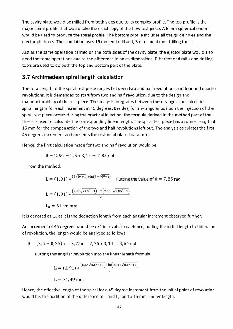
47
The cavity plate would be milled from both sides due to its complex profile. The top profile is the
major spiral profile that would take the exact copy of the flow test piece. A 6 mm spherical end mill
would be used to produce the spiral profile. The bottom profile includes all the guide holes and the
ejector pin holes. The simulation uses 16 mm end mill and, 3 mm and 4 mm drilling tools.
Just as the same operation carried on the both sides of the cavity plate, the ejector plate would also
need the same operations due to the difference in holes dimensions. Different end mills and drilling
tools are used to do both the top and bottom part of the plate.
3.7 Archimedean spiral length calculation
The total length of the spiral test piece ranges between two and half revolutions and four and quarter
revolutions. It is demanded to start from two and half revolution, due to the design and
manufacturability of the test piece. The analysis integrates between these ranges and calculates
spiral lengths for each increment in 45 degrees. Besides, for any angular position the injection of the
spiral test piece occurs during the practical injection, the formula derived in the method part of the
thesis is used to calculate the corresponding linear length. The spiral test piece has a runner length of
15 mm for the compensation of the two and half revolutions left out. The analysis calculates the first
45 degrees increment and presents the rest in tabulated data form.
Hence, the first calculation made for two and half revolution would be;
rad
From the method,
( ) ( √ ) ( √ )
Putting the value of rad
( ) ( √ ) ( √ )
It is denoted as Lo, as it is the deduction length from each angular increment observed further.
An increment of 45 degrees would be π/4 in revolutions. Hence, adding the initial length to this value
of revolution, the length would be analysed as follows,
( ) rad
Putting this angular revolution into the linear length formula,
( ) ( √ ) ( √ )
Hence, the effective length of the spiral for a 45 degree increment from the initial point of revolution
would be, the addition of the difference of L and Lo, and a 15 mm runner length,
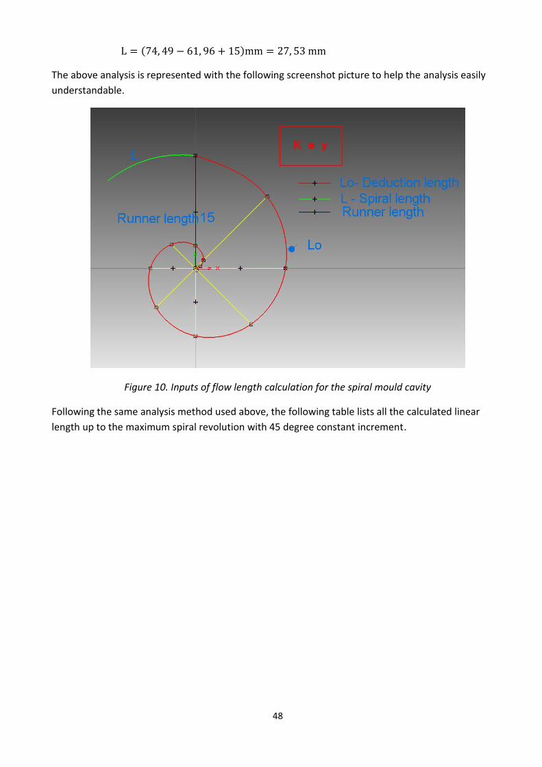
48
( )
The above analysis is represented with the following screenshot picture to help the analysis easily
understandable.
Figure 10. Inputs of flow length calculation for the spiral mould cavity
Following the same analysis method used above, the following table lists all the calculated linear
length up to the maximum spiral revolution with 45 degree constant increment.
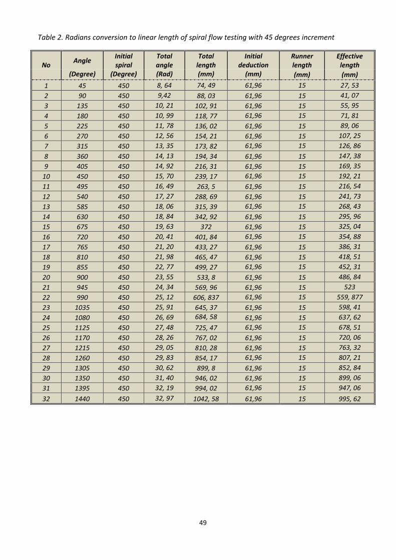
49
Table 2. Radians conversion to linear length of spiral flow testing with 45 degrees increment
No Angle
Initial spiral
Total angle
Total length
Initial deduction
Runner length
Effective length
(Degree) (Degree) (Rad) (mm) (mm) (mm) (mm)
1 45 450 8, 64 74, 49 61,96 15 27, 53
2 90 450 9,42 88, 03 61,96 15 41, 07
3 135 450 10, 21 102, 91 61,96 15 55, 95
4 180 450 10, 99 118, 77 61,96 15 71, 81
5 225 450 11, 78 136, 02 61,96 15 89, 06
6 270 450 12, 56 154, 21 61,96 15 107, 25
7 315 450 13, 35 173, 82 61,96 15 126, 86
8 360 450 14, 13 194, 34 61,96 15 147, 38
9 405 450 14, 92 216, 31 61,96 15 169, 35
10 450 450 15, 70 239, 17 61,96 15 192, 21
11 495 450 16, 49 263, 5 61,96 15 216, 54
12 540 450 17, 27 288, 69 61,96 15 241, 73
13 585 450 18, 06 315, 39 61,96 15 268, 43
14 630 450 18, 84 342, 92 61,96 15 295, 96
15 675 450 19, 63 372 61,96 15 325, 04
16 720 450 20, 41 401, 84 61,96 15 354, 88
17 765 450 21, 20 433, 27 61,96 15 386, 31
18 810 450 21, 98 465, 47 61,96 15 418, 51
19 855 450 22, 77 499, 27 61,96 15 452, 31
20 900 450 23, 55 533, 8 61,96 15 486, 84
21 945 450 24, 34 569, 96 61,96 15 523
22 990 450 25, 12 606, 837 61,96 15 559, 877
23 1035 450 25, 91 645, 37 61,96 15 598, 41
24 1080 450 26, 69 684, 58 61,96 15 637, 62
25 1125 450 27, 48 725, 47 61,96 15 678, 51
26 1170 450 28, 26 767, 02 61,96 15 720, 06
27 1215 450 29, 05 810, 28 61,96 15 763, 32
28 1260 450 29, 83 854, 17 61,96 15 807, 21
29 1305 450 30, 62 899, 8 61,96 15 852, 84
30 1350 450 31, 40 946, 02 61,96 15 899, 06
31 1395 450 32, 19 994, 02 61,96 15 947, 06
32 1440 450 32, 97 1042, 58 61,96 15 995, 62
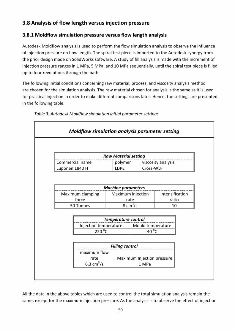
50
3.8 Analysis of flow length versus injection pressure
3.8.1 Moldflow simulation pressure versus flow length analysis
Autodesk Moldflow analysis is used to perform the flow simulation analysis to observe the influence
of injection pressure on flow length. The spiral test piece is imported to the Autodesk synergy from
the prior design made on SolidWorks software. A study of fill analysis is made with the increment of
injection pressure ranges in 1 MPa, 5 MPa, and 10 MPa sequentially, until the spiral test piece is filled
up to four revolutions through the path.
The following initial conditions concerning raw material, process, and viscosity analysis method
are chosen for the simulation analysis. The raw material chosen for analysis is the same as it is used
for practical injection in order to make different comparisons later. Hence, the settings are presented
in the following table.
Table 3. Autodesk Moldflow simulation initial parameter settings
Moldflow simulation analysis parameter setting
Raw Material setting
Commercial name polymer viscosity analysis
Luponen 1840 H LDPE Cross-WLF
Machine parameters
Maximum clamping force
Maximum injection rate
Intensification ratio
50 Tonnes 8 cm3/s 10
Temperature control
Injection temperature Mould temperature
220 oC 40 oC
Filling control
maximum flow rate Maximum Injection pressure
6,3 cm3/s 1 MPa
All the data in the above tables which are used to control the total simulation analysis remain the
same, except for the maximum injection pressure. As the analysis is to observe the effect of injection
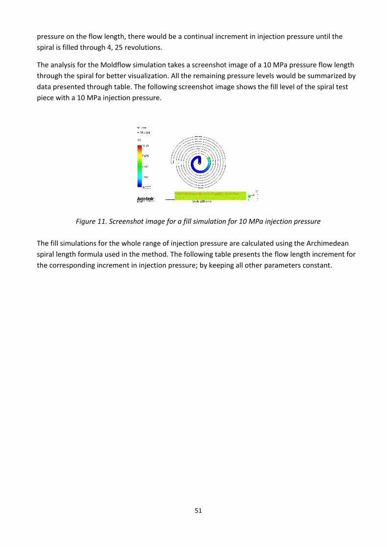
51
pressure on the flow length, there would be a continual increment in injection pressure until the
spiral is filled through 4, 25 revolutions.
The analysis for the Moldflow simulation takes a screenshot image of a 10 MPa pressure flow length
through the spiral for better visualization. All the remaining pressure levels would be summarized by
data presented through table. The following screenshot image shows the fill level of the spiral test
piece with a 10 MPa injection pressure.
Figure 11. Screenshot image for a fill simulation for 10 MPa injection pressure
The fill simulations for the whole range of injection pressure are calculated using the Archimedean
spiral length formula used in the method. The following table presents the flow length increment for
the corresponding increment in injection pressure; by keeping all other parameters constant.
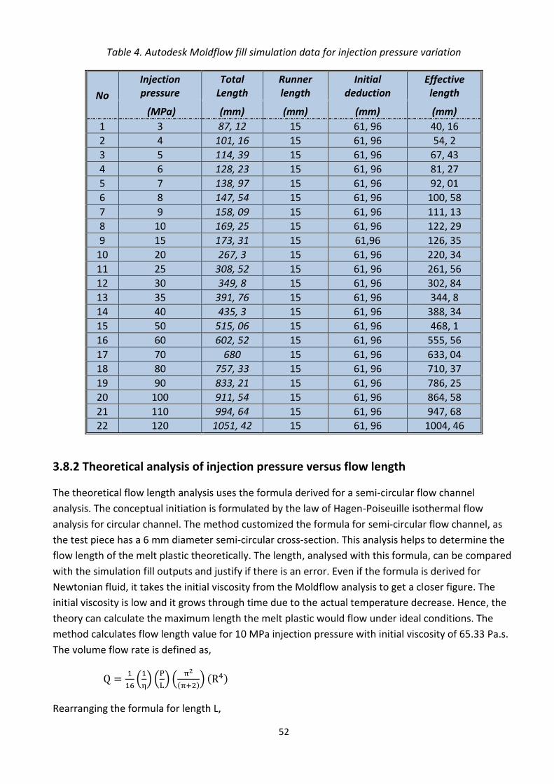
52
Table 4. Autodesk Moldflow fill simulation data for injection pressure variation
No
Injection pressure
Total Length
Runner length
Initial deduction
Effective length
(MPa) (mm) (mm) (mm) (mm)
1 3 87, 12 15 61, 96 40, 16
2 4 101, 16 15 61, 96 54, 2
3 5 114, 39 15 61, 96 67, 43
4 6 128, 23 15 61, 96 81, 27
5 7 138, 97 15 61, 96 92, 01
6 8 147, 54 15 61, 96 100, 58
7 9 158, 09 15 61, 96 111, 13
8 10 169, 25 15 61, 96 122, 29
9 15 173, 31 15 61,96 126, 35
10 20 267, 3 15 61, 96 220, 34
11 25 308, 52 15 61, 96 261, 56
12 30 349, 8 15 61, 96 302, 84
13 35 391, 76 15 61, 96 344, 8
14 40 435, 3 15 61, 96 388, 34
15 50 515, 06 15 61, 96 468, 1
16 60 602, 52 15 61, 96 555, 56
17 70 680 15 61, 96 633, 04
18 80 757, 33 15 61, 96 710, 37
19 90 833, 21 15 61, 96 786, 25
20 100 911, 54 15 61, 96 864, 58
21 110 994, 64 15 61, 96 947, 68
22 120 1051, 42 15 61, 96 1004, 46
3.8.2 Theoretical analysis of injection pressure versus flow length
The theoretical flow length analysis uses the formula derived for a semi-circular flow channel
analysis. The conceptual initiation is formulated by the law of Hagen-Poiseuille isothermal flow
analysis for circular channel. The method customized the formula for semi-circular flow channel, as
the test piece has a 6 mm diameter semi-circular cross-section. This analysis helps to determine the
flow length of the melt plastic theoretically. The length, analysed with this formula, can be compared
with the simulation fill outputs and justify if there is an error. Even if the formula is derived for
Newtonian fluid, it takes the initial viscosity from the Moldflow analysis to get a closer figure. The
initial viscosity is low and it grows through time due to the actual temperature decrease. Hence, the
theory can calculate the maximum length the melt plastic would flow under ideal conditions. The
method calculates flow length value for 10 MPa injection pressure with initial viscosity of 65.33 Pa.s.
The volume flow rate is defined as,
(
) (
) (
( )) ( )
Rearranging the formula for length L,
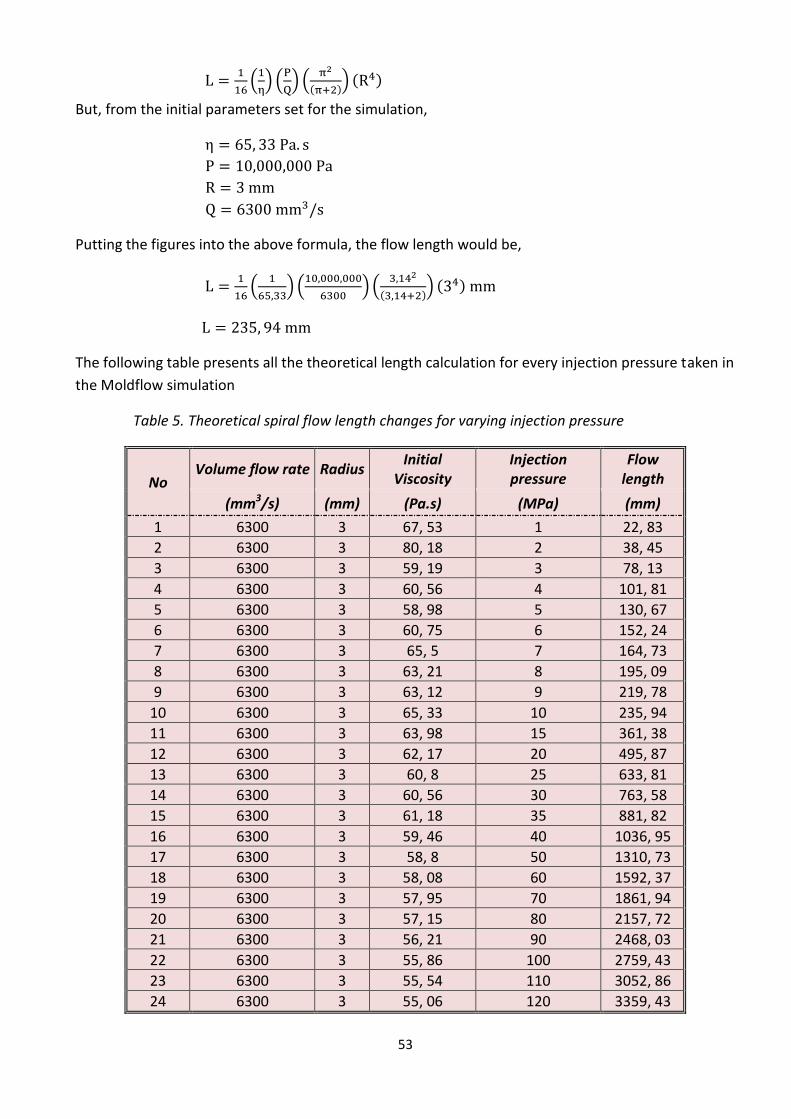
53
(
) (
) (
( )) ( )
But, from the initial parameters set for the simulation,
Putting the figures into the above formula, the flow length would be,
(
) (
) (
( )) ( )
The following table presents all the theoretical length calculation for every injection pressure taken in
the Moldflow simulation
Table 5. Theoretical spiral flow length changes for varying injection pressure
No Volume flow rate Radius
Initial Viscosity
Injection pressure
Flow length
(mm3/s) (mm) (Pa.s) (MPa) (mm)
1 6300 3 67, 53 1 22, 83
2 6300 3 80, 18 2 38, 45
3 6300 3 59, 19 3 78, 13
4 6300 3 60, 56 4 101, 81
5 6300 3 58, 98 5 130, 67
6 6300 3 60, 75 6 152, 24
7 6300 3 65, 5 7 164, 73
8 6300 3 63, 21 8 195, 09
9 6300 3 63, 12 9 219, 78
10 6300 3 65, 33 10 235, 94
11 6300 3 63, 98 15 361, 38
12 6300 3 62, 17 20 495, 87
13 6300 3 60, 8 25 633, 81
14 6300 3 60, 56 30 763, 58
15 6300 3 61, 18 35 881, 82
16 6300 3 59, 46 40 1036, 95
17 6300 3 58, 8 50 1310, 73
18 6300 3 58, 08 60 1592, 37
19 6300 3 57, 95 70 1861, 94
20 6300 3 57, 15 80 2157, 72
21 6300 3 56, 21 90 2468, 03
22 6300 3 55, 86 100 2759, 43
23 6300 3 55, 54 110 3052, 86
24 6300 3 55, 06 120 3359, 43
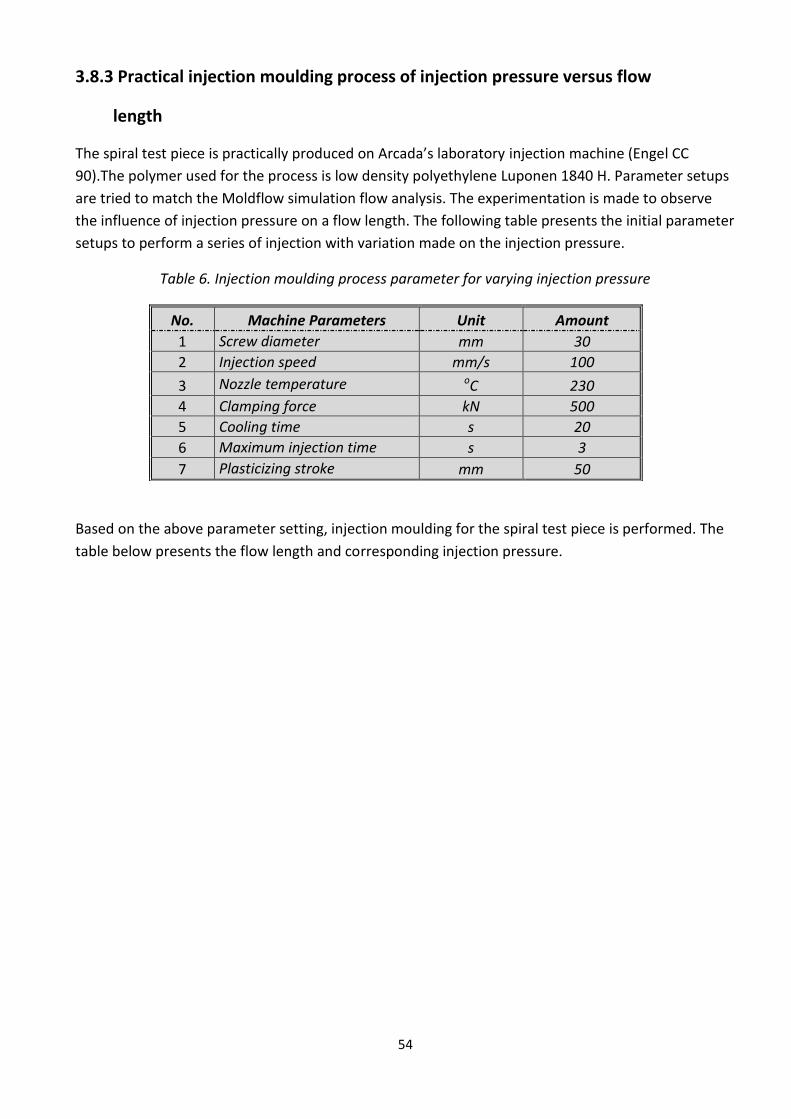
54
3.8.3 Practical injection moulding process of injection pressure versus flow
length
The spiral test piece is practically produced on Arcada’s laboratory injection machine (Engel CC
90).The polymer used for the process is low density polyethylene Luponen 1840 H. Parameter setups
are tried to match the Moldflow simulation flow analysis. The experimentation is made to observe
the influence of injection pressure on a flow length. The following table presents the initial parameter
setups to perform a series of injection with variation made on the injection pressure.
Table 6. Injection moulding process parameter for varying injection pressure
Based on the above parameter setting, injection moulding for the spiral test piece is performed. The
table below presents the flow length and corresponding injection pressure.
No. Machine Parameters Unit Amount
1 Screw diameter mm 30
2 Injection speed mm/s 100
3 Nozzle temperature oC 230
4 Clamping force kN 500
5 Cooling time s 20
6 Maximum injection time s 3
7 Plasticizing stroke mm 50
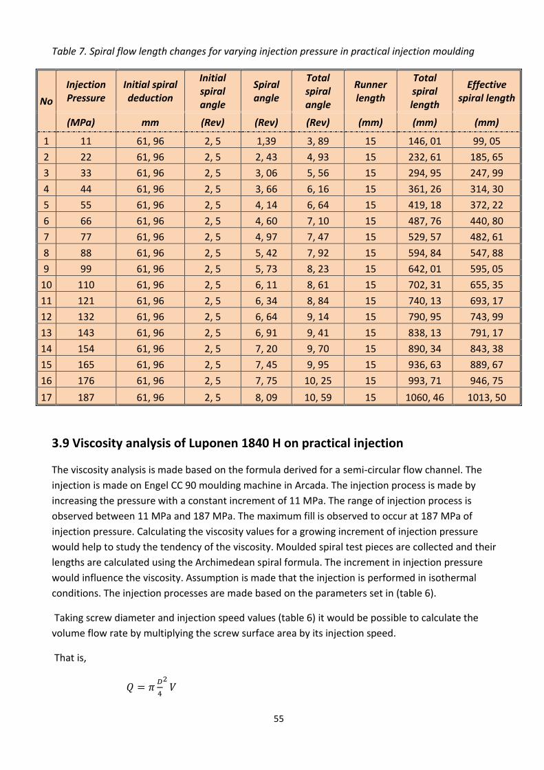
55
Table 7. Spiral flow length changes for varying injection pressure in practical injection moulding
No
Injection Pressure
Initial spiral deduction
Initial spiral angle
Spiral angle
Total spiral angle
Runner length
Total spiral length
Effective spiral length
(MPa) mm (Rev) (Rev) (Rev) (mm) (mm) (mm)
1 11 61, 96 2, 5 1,39 3, 89 15 146, 01 99, 05
2 22 61, 96 2, 5 2, 43 4, 93 15 232, 61 185, 65
3 33 61, 96 2, 5 3, 06 5, 56 15 294, 95 247, 99
4 44 61, 96 2, 5 3, 66 6, 16 15 361, 26 314, 30
5 55 61, 96 2, 5 4, 14 6, 64 15 419, 18 372, 22
6 66 61, 96 2, 5 4, 60 7, 10 15 487, 76 440, 80
7 77 61, 96 2, 5 4, 97 7, 47 15 529, 57 482, 61
8 88 61, 96 2, 5 5, 42 7, 92 15 594, 84 547, 88
9 99 61, 96 2, 5 5, 73 8, 23 15 642, 01 595, 05
10 110 61, 96 2, 5 6, 11 8, 61 15 702, 31 655, 35
11 121 61, 96 2, 5 6, 34 8, 84 15 740, 13 693, 17
12 132 61, 96 2, 5 6, 64 9, 14 15 790, 95 743, 99
13 143 61, 96 2, 5 6, 91 9, 41 15 838, 13 791, 17
14 154 61, 96 2, 5 7, 20 9, 70 15 890, 34 843, 38
15 165 61, 96 2, 5 7, 45 9, 95 15 936, 63 889, 67
16 176 61, 96 2, 5 7, 75 10, 25 15 993, 71 946, 75
17 187 61, 96 2, 5 8, 09 10, 59 15 1060, 46 1013, 50
3.9 Viscosity analysis of Luponen 1840 H on practical injection
The viscosity analysis is made based on the formula derived for a semi-circular flow channel. The
injection is made on Engel CC 90 moulding machine in Arcada. The injection process is made by
increasing the pressure with a constant increment of 11 MPa. The range of injection process is
observed between 11 MPa and 187 MPa. The maximum fill is observed to occur at 187 MPa of
injection pressure. Calculating the viscosity values for a growing increment of injection pressure
would help to study the tendency of the viscosity. Moulded spiral test pieces are collected and their
lengths are calculated using the Archimedean spiral formula. The increment in injection pressure
would influence the viscosity. Assumption is made that the injection is performed in isothermal
conditions. The injection processes are made based on the parameters set in (table 6).
Taking screw diameter and injection speed values (table 6) it would be possible to calculate the
volume flow rate by multiplying the screw surface area by its injection speed.
That is,
56
Where, V is injection speed (mm)
Putting the values,
( )
(
)
The first injection made with 11 MPa of injection pressure would be calculated using the formula and
the rest consecutive pressure increments are summarized with a table.
Taking the isothermal flow formula,
(
) (
) (
( )) ( )
Rearranging the formula,
(
) (
) (
( )) ( )
Here, from the practical injection, the length of the spiral for the corresponding 11 MPa injection
pressure is 99, 05 mm.
(
) (
) (
( )) ( )
(
) (
) (
( )) ( )
And the rest of viscosities, analysed through the above method, are presented in the following table.
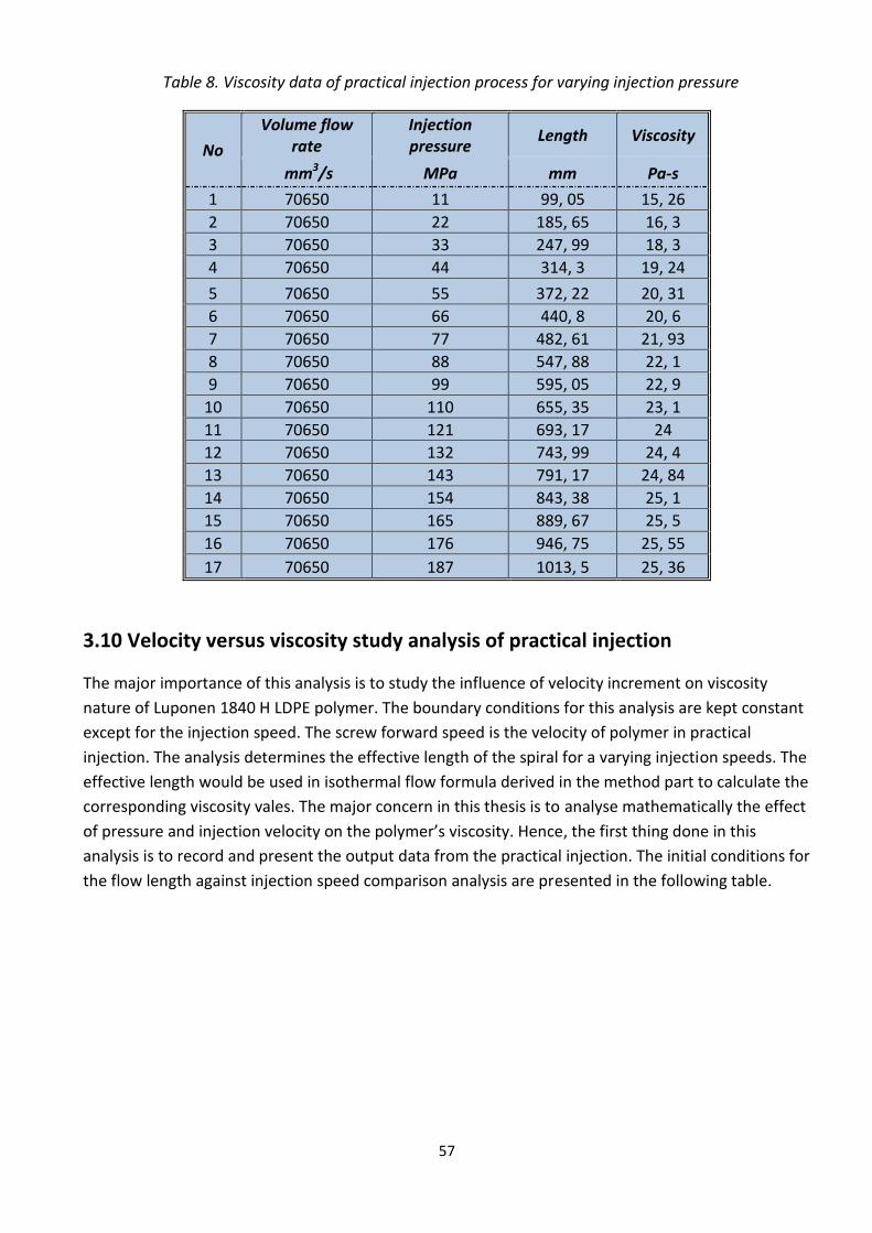
57
Table 8. Viscosity data of practical injection process for varying injection pressure
No
Volume flow rate
Injection pressure
Length Viscosity
mm3/s MPa mm Pa-s
1 70650 11 99, 05 15, 26
2 70650 22 185, 65 16, 3
3 70650 33 247, 99 18, 3
4 70650 44 314, 3 19, 24
5 70650 55 372, 22 20, 31
6 70650 66 440, 8 20, 6
7 70650 77 482, 61 21, 93
8 70650 88 547, 88 22, 1
9 70650 99 595, 05 22, 9
10 70650 110 655, 35 23, 1
11 70650 121 693, 17 24
12 70650 132 743, 99 24, 4
13 70650 143 791, 17 24, 84
14 70650 154 843, 38 25, 1
15 70650 165 889, 67 25, 5
16 70650 176 946, 75 25, 55
17 70650 187 1013, 5 25, 36
3.10 Velocity versus viscosity study analysis of practical injection
The major importance of this analysis is to study the influence of velocity increment on viscosity
nature of Luponen 1840 H LDPE polymer. The boundary conditions for this analysis are kept constant
except for the injection speed. The screw forward speed is the velocity of polymer in practical
injection. The analysis determines the effective length of the spiral for a varying injection speeds. The
effective length would be used in isothermal flow formula derived in the method part to calculate the
corresponding viscosity vales. The major concern in this thesis is to analyse mathematically the effect
of pressure and injection velocity on the polymer’s viscosity. Hence, the first thing done in this
analysis is to record and present the output data from the practical injection. The initial conditions for
the flow length against injection speed comparison analysis are presented in the following table.
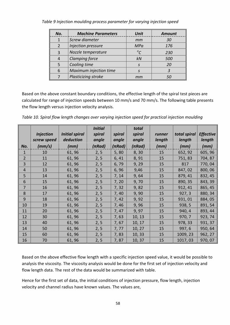
58
Table 9 Injection moulding process parameter for varying injection speed
No. Machine Parameters Unit Amount
1 Screw diameter mm 30
2 Injection pressure MPa 176
3 Nozzle temperature oC 230
4 Clamping force kN 500
5 Cooling time s 20
6 Maximum injection time s 3
7 Plasticizing stroke mm 50
Based on the above constant boundary conditions, the effective length of the spiral test pieces are
calculated for range of injection speeds between 10 mm/s and 70 mm/s. The following table presents
the flow length versus injection velocity analysis.
Table 10. Spiral flow length changes over varying injection speed for practical injection moulding
No.
Injection screw speed
Initial spiral deduction
Initial spiral angle
spiral angle
total spiral angle
runner length
total spiral length
Effective length
(mm/s) (mm) (πRad) (πRad) (πRad) (mm) (mm) (mm)
1 10 61, 96 2, 5 5, 80 8, 30 15 652, 92 605, 96
2 11 61, 96 2, 5 6, 41 8, 91 15 751, 83 704, 87
3 12 61, 96 2, 5 6, 79 9, 29 15 817 770, 04
4 13 61, 96 2, 5 6, 96 9,46 15 847, 02 800, 06
5 14 61, 96 2, 5 7, 14 9, 64 15 879, 41 832, 45
6 15 61, 96 2, 5 7, 20 9, 70 15 890, 35 843, 39
7 16 61, 96 2, 5 7, 32 9, 82 15 912, 41 865, 45
8 17 61, 96 2, 5 7, 40 9, 90 15 927, 3 880, 34
9 18 61, 96 2, 5 7, 42 9, 92 15 931, 01 884, 05
10 19 61, 96 2, 5 7, 46 9, 96 15 938, 5 891, 54
11 20 61, 96 2, 5 7, 47 9, 97 15 940, 4 893, 44
12 30 61, 96 2, 5 7, 63 10, 13 15 970, 7 923, 74
13 40 61, 96 2, 5 7, 67 10, 17 15 978, 33 931, 37
14 50 61, 96 2, 5 7, 77 10, 27 15 997, 6 950, 64
15 60 61, 96 2, 5 7, 83 10, 33 15 1009, 23 962, 27
16 70 61, 96 2, 5 7, 87 10, 37 15 1017, 03 970, 07
Based on the above effective flow length with a specific injection speed value, it would be possible to
analysis the viscosity. The viscosity analysis would be done for the first set of injection velocity and
flow length data. The rest of the data would be summarized with table.
Hence for the first set of data, the initial conditions of injection pressure, flow length, injection
velocity and channel radius have known values. The values are,
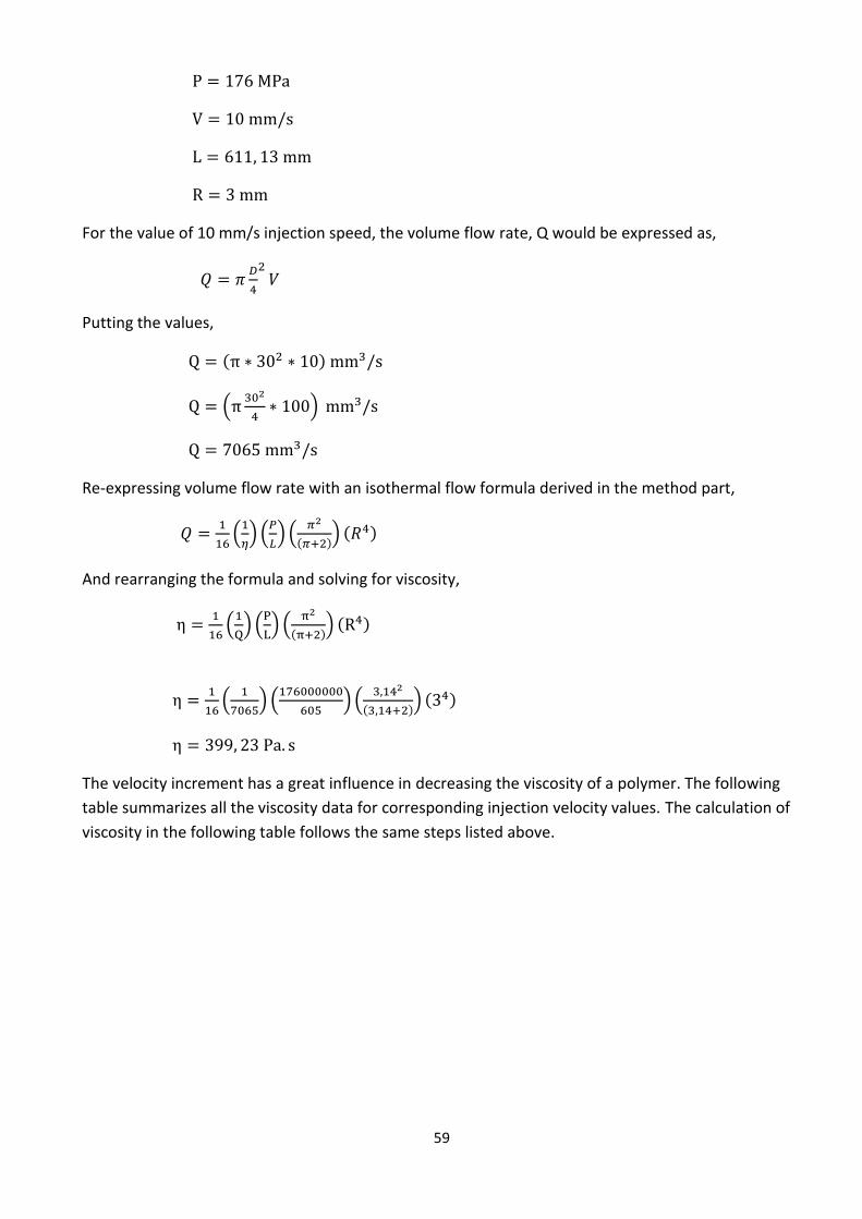
59
For the value of 10 mm/s injection speed, the volume flow rate, Q would be expressed as,
Putting the values,
( )
(
)
Re-expressing volume flow rate with an isothermal flow formula derived in the method part,
(
) (
) (
( )) ( )
And rearranging the formula and solving for viscosity,
(
) (
) (
( )) ( )
(
) (
) (
( )) ( )
The velocity increment has a great influence in decreasing the viscosity of a polymer. The following
table summarizes all the viscosity data for corresponding injection velocity values. The calculation of
viscosity in the following table follows the same steps listed above.
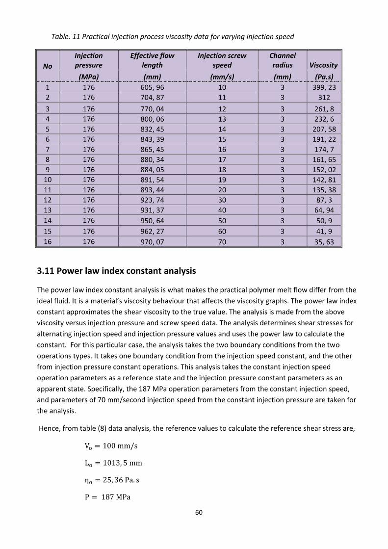
60
Table. 11 Practical injection process viscosity data for varying injection speed
No
Injection pressure
Effective flow length
Injection screw speed
Channel radius Viscosity
(MPa) (mm) (mm/s) (mm) (Pa.s)
1 176 605, 96 10 3 399, 23
2 176 704, 87 11 3 312
3 176 770, 04 12 3 261, 8
4 176 800, 06 13 3 232, 6
5 176 832, 45 14 3 207, 58
6 176 843, 39 15 3 191, 22
7 176 865, 45 16 3 174, 7
8 176 880, 34 17 3 161, 65
9 176 884, 05 18 3 152, 02
10 176 891, 54 19 3 142, 81
11 176 893, 44 20 3 135, 38
12 176 923, 74 30 3 87, 3
13 176 931, 37 40 3 64, 94
14 176 950, 64 50 3 50, 9
15 176 962, 27 60 3 41, 9
16 176 970, 07 70 3 35, 63
3.11 Power law index constant analysis
The power law index constant analysis is what makes the practical polymer melt flow differ from the
ideal fluid. It is a material’s viscosity behaviour that affects the viscosity graphs. The power law index
constant approximates the shear viscosity to the true value. The analysis is made from the above
viscosity versus injection pressure and screw speed data. The analysis determines shear stresses for
alternating injection speed and injection pressure values and uses the power law to calculate the
constant. For this particular case, the analysis takes the two boundary conditions from the two
operations types. It takes one boundary condition from the injection speed constant, and the other
from injection pressure constant operations. This analysis takes the constant injection speed
operation parameters as a reference state and the injection pressure constant parameters as an
apparent state. Specifically, the 187 MPa operation parameters from the constant injection speed,
and parameters of 70 mm/second injection speed from the constant injection pressure are taken for
the analysis.
Hence, from table (8) data analysis, the reference values to calculate the reference shear stress are,
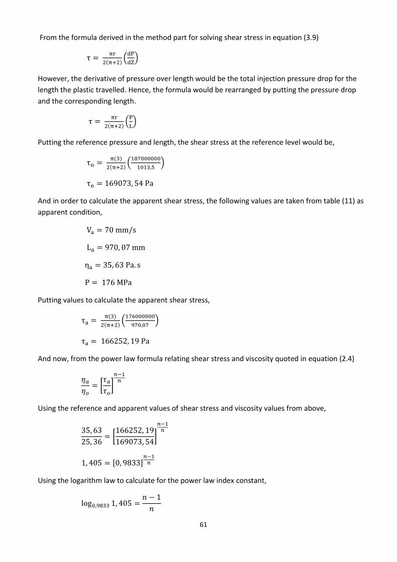
61
From the formula derived in the method part for solving shear stress in equation (3.9)
( )(
)
However, the derivative of pressure over length would be the total injection pressure drop for the
length the plastic travelled. Hence, the formula would be rearranged by putting the pressure drop
and the corresponding length.
( )(
)
Putting the reference pressure and length, the shear stress at the reference level would be,
( )
( )(
)
And in order to calculate the apparent shear stress, the following values are taken from table (11) as
apparent condition,
Putting values to calculate the apparent shear stress,
( )
( )(
)
And now, from the power law formula relating shear stress and viscosity quoted in equation (2.4)
[
]
Using the reference and apparent values of shear stress and viscosity values from above,
[
]
[ ]
Using the logarithm law to calculate for the power law index constant,
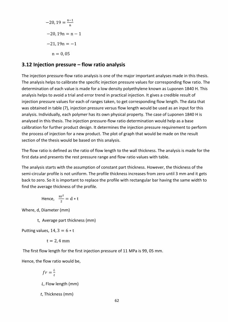
62
3.12 Injection pressure – flow ratio analysis
The injection pressure-flow ratio analysis is one of the major important analyses made in this thesis.
The analysis helps to calibrate the specific injection pressure values for corresponding flow ratio. The
determination of each value is made for a low density polyethylene known as Luponen 1840 H. This
analysis helps to avoid a trial and error trend in practical injection. It gives a credible result of
injection pressure values for each of ranges taken, to get corresponding flow length. The data that
was obtained in table (7), injection pressure versus flow length would be used as an input for this
analysis. Individually, each polymer has its own physical property. The case of Luponen 1840 H is
analysed in this thesis. The injection pressure-flow ratio determination would help as a base
calibration for further product design. It determines the injection pressure requirement to perform
the process of injection for a new product. The plot of graph that would be made on the result
section of the thesis would be based on this analysis.
The flow ratio is defined as the ratio of flow length to the wall thickness. The analysis is made for the
first data and presents the rest pressure range and flow ratio values with table.
The analysis starts with the assumption of constant part thickness. However, the thickness of the
semi-circular profile is not uniform. The profile thickness increases from zero until 3 mm and it gets
back to zero. So it is important to replace the profile with rectangular bar having the same width to
find the average thickness of the profile.
Hence,
Where, d, Diameter (mm)
t, Average part thickness (mm)
Putting values,
The first flow length for the first injection pressure of 11 MPa is 99, 05 mm.
Hence, the flow ratio would be,
L, Flow length (mm)
t, Thickness (mm)
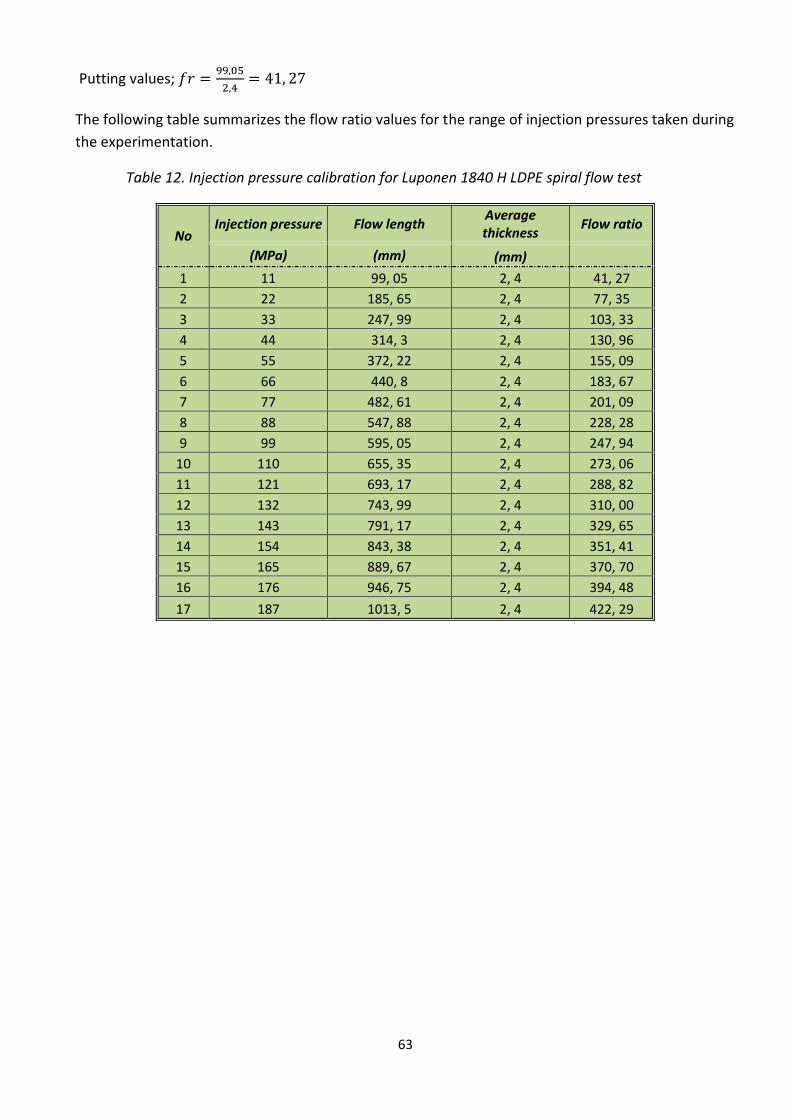
63
Putting values;
The following table summarizes the flow ratio values for the range of injection pressures taken during
the experimentation.
Table 12. Injection pressure calibration for Luponen 1840 H LDPE spiral flow test
No Injection pressure Flow length
Average thickness
Flow ratio
(MPa) (mm) (mm)
1 11 99, 05 2, 4 41, 27
2 22 185, 65 2, 4 77, 35
3 33 247, 99 2, 4 103, 33
4 44 314, 3 2, 4 130, 96
5 55 372, 22 2, 4 155, 09
6 66 440, 8 2, 4 183, 67
7 77 482, 61 2, 4 201, 09
8 88 547, 88 2, 4 228, 28
9 99 595, 05 2, 4 247, 94
10 110 655, 35 2, 4 273, 06
11 121 693, 17 2, 4 288, 82
12 132 743, 99 2, 4 310, 00
13 143 791, 17 2, 4 329, 65
14 154 843, 38 2, 4 351, 41
15 165 889, 67 2, 4 370, 70
16 176 946, 75 2, 4 394, 48
17 187 1013, 5 2, 4 422, 29
64
4. RESULTS
4.1 Result Summary The result summary part of the thesis comprises of all of the work performed in this thesis. The thesis
started with performing the mould design, analysis, manufacturing and theoretical formulations
governing the work. Data are also collected and interpreted into graphs in order to make
understandable comparison of different operation conditions. Ranges of different analyses have been
performed in the method section of the thesis. The outputs of all these analyses are presented in this
section of the thesis.
Generally, the following works have been completed and briefly explained with illustrations in this
section of the thesis.
4.1.1 Spiral flow testing mould design
4.1.2 Spiral flow test piece design
4.1.3 Autodesk Moldflow simulation for plastic injection of the spiral flow test
4.1.4 Mastercam design and mill for all mould plates
4.1.5 Complete Spiral mould set manufacturing on Haas Mill
4.1.6 Isothermal flow formula for semi-circular channel
4.1.7 Spiral flow test manufacturing for different operation parameters
4.1.8 Comparison of Injection pressure versus flow length data for theoretical, simulation and
practical injection
4.1.9 Viscosity calculations for varying injection pressure and injection speed values on practical
injection
4.1.10 Comparisons of parameter change influences on viscosity through injection speed and
injection pressure.
4.1.11 Calculate the power law index constant for Luponen 1840 H LDPE polymer
4.1.12 Calibration injection pressure for Luponen 1840 H LDPE based on the flow ratio
The result part of the thesis would illustrate the above works performed through different snapshots,
design features, photographs and graphs to clearly show the task. Each of the above listed tasks
would be observed in detail below.
4.1.1 Spiral flow testing mould design
As mentioned in the method section, the Solid Edge modelling is used to design the mould set. The
156 *156 mm2 standard plate is used to design the mould set. The following three dimensional
modelling shows the complete mould set.
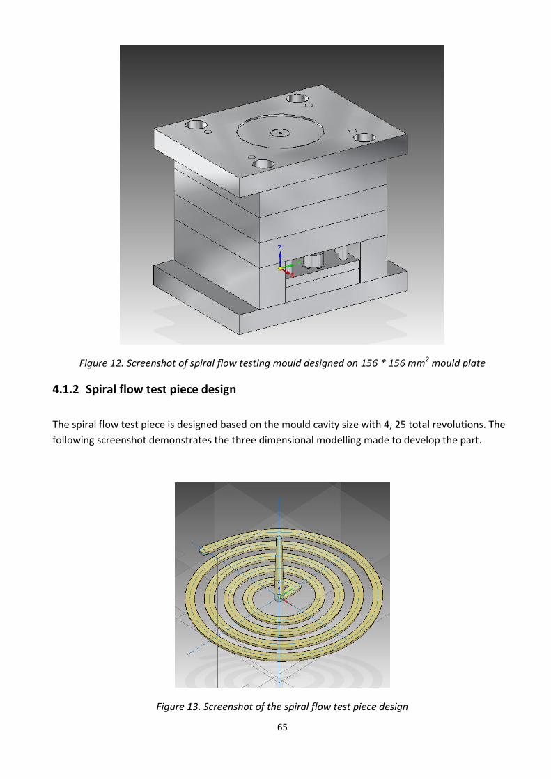
65
Figure 12. Screenshot of spiral flow testing mould designed on 156 * 156 mm2 mould plate
4.1.2 Spiral flow test piece design
The spiral flow test piece is designed based on the mould cavity size with 4, 25 total revolutions. The
following screenshot demonstrates the three dimensional modelling made to develop the part.
Figure 13. Screenshot of the spiral flow test piece design
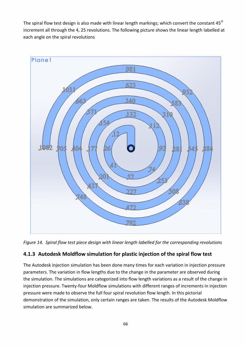
66
The spiral flow test design is also made with linear length markings; which convert the constant 45O
increment all through the 4, 25 revolutions. The following picture shows the linear length labelled at
each angle on the spiral revolutions
Figure 14. Spiral flow test piece design with linear length labelled for the corresponding revolutions
4.1.3 Autodesk Moldflow simulation for plastic injection of the spiral flow test The Autodesk injection simulation has been done many times for each variation in injection pressure
parameters. The variation in flow lengths due to the change in the parameter are observed during
the simulation. The simulations are categorized into flow length variations as a result of the change in
injection pressure. Twenty-four Moldflow simulations with different ranges of increments in injection
pressure were made to observe the full four spiral revolution flow length. In this pictorial
demonstration of the simulation, only certain ranges are taken. The results of the Autodesk Moldflow
simulation are summarized below.
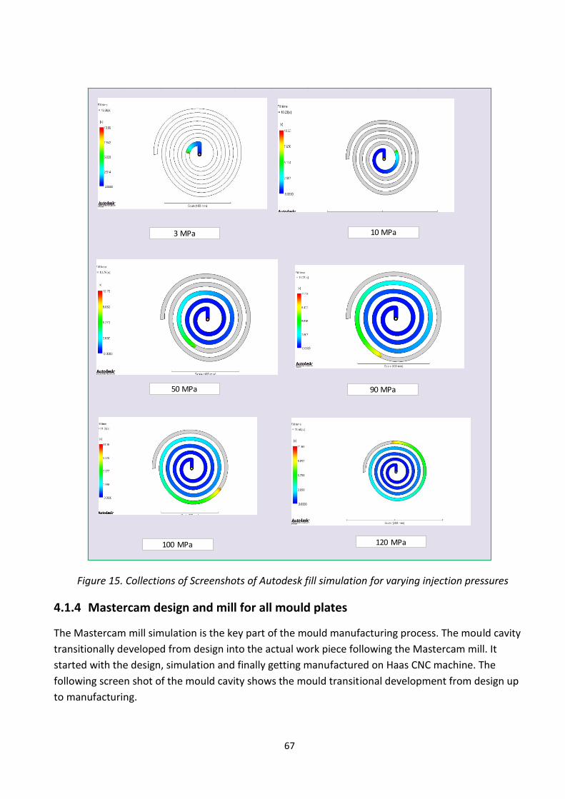
67
Figure 15. Collections of Screenshots of Autodesk fill simulation for varying injection pressures
4.1.4 Mastercam design and mill for all mould plates The Mastercam mill simulation is the key part of the mould manufacturing process. The mould cavity
transitionally developed from design into the actual work piece following the Mastercam mill. It
started with the design, simulation and finally getting manufactured on Haas CNC machine. The
following screen shot of the mould cavity shows the mould transitional development from design up
to manufacturing.
3 MPa 10 MPa
50 MPa 90 MPa
100 MPa 120 MPa
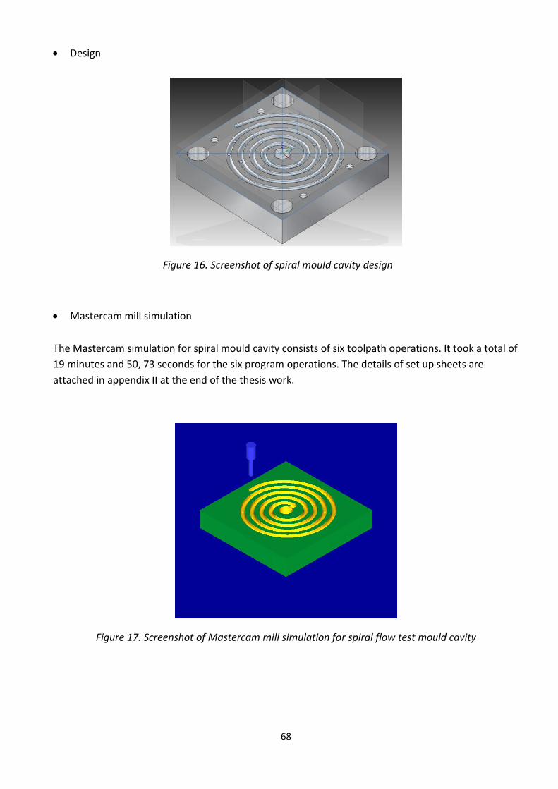
68
Design
Figure 16. Screenshot of spiral mould cavity design
Mastercam mill simulation
The Mastercam simulation for spiral mould cavity consists of six toolpath operations. It took a total of
19 minutes and 50, 73 seconds for the six program operations. The details of set up sheets are
attached in appendix II at the end of the thesis work.
Figure 17. Screenshot of Mastercam mill simulation for spiral flow test mould cavity
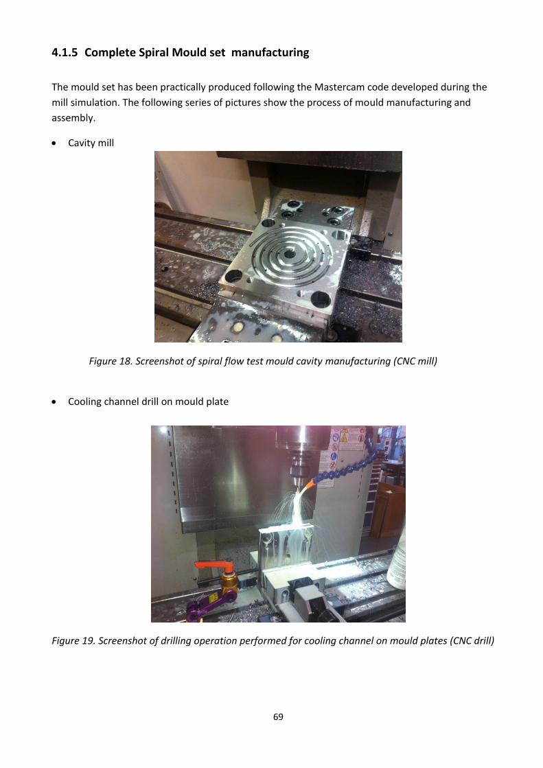
69
4.1.5 Complete Spiral Mould set manufacturing
The mould set has been practically produced following the Mastercam code developed during the
mill simulation. The following series of pictures show the process of mould manufacturing and
assembly.
Cavity mill
Figure 18. Screenshot of spiral flow test mould cavity manufacturing (CNC mill)
Cooling channel drill on mould plate
Figure 19. Screenshot of drilling operation performed for cooling channel on mould plates (CNC drill)
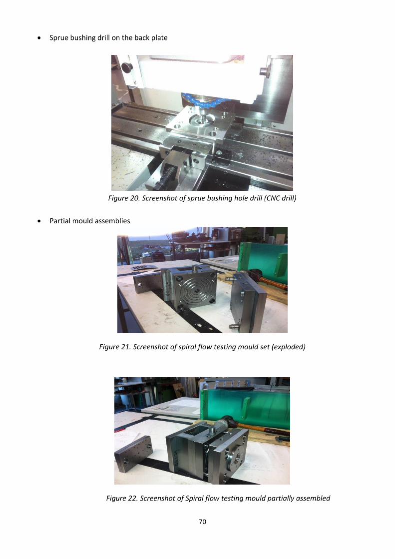
70
Sprue bushing drill on the back plate
Figure 20. Screenshot of sprue bushing hole drill (CNC drill)
Partial mould assemblies
Figure 21. Screenshot of spiral flow testing mould set (exploded)
Figure 22. Screenshot of Spiral flow testing mould partially assembled
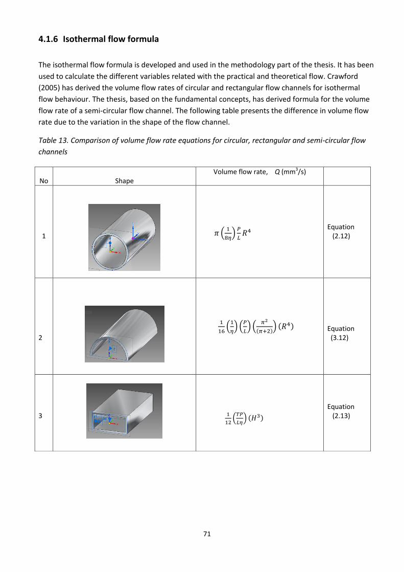
71
4.1.6 Isothermal flow formula
The isothermal flow formula is developed and used in the methodology part of the thesis. It has been
used to calculate the different variables related with the practical and theoretical flow. Crawford
(2005) has derived the volume flow rates of circular and rectangular flow channels for isothermal
flow behaviour. The thesis, based on the fundamental concepts, has derived formula for the volume
flow rate of a semi-circular flow channel. The following table presents the difference in volume flow
rate due to the variation in the shape of the flow channel.
Table 13. Comparison of volume flow rate equations for circular, rectangular and semi-circular flow
channels
No
Shape
Volume flow rate, Q (mm3/s)
1
(
)
Equation (2.12)
2
(
) (
) (
( )) ( )
Equation (3.12)
3
(
) ( )
Equation (2.13)
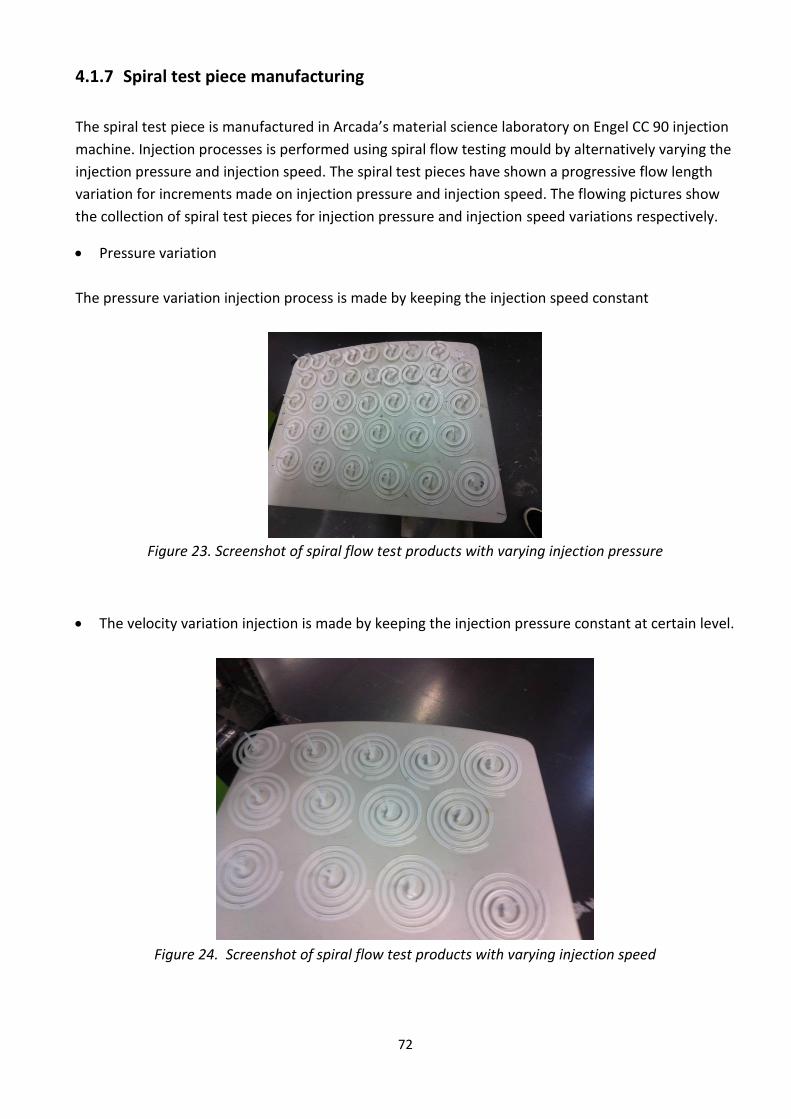
72
4.1.7 Spiral test piece manufacturing
The spiral test piece is manufactured in Arcada’s material science laboratory on Engel CC 90 injection
machine. Injection processes is performed using spiral flow testing mould by alternatively varying the
injection pressure and injection speed. The spiral test pieces have shown a progressive flow length
variation for increments made on injection pressure and injection speed. The flowing pictures show
the collection of spiral test pieces for injection pressure and injection speed variations respectively.
Pressure variation
The pressure variation injection process is made by keeping the injection speed constant
Figure 23. Screenshot of spiral flow test products with varying injection pressure
The velocity variation injection is made by keeping the injection pressure constant at certain level.
Figure 24. Screenshot of spiral flow test products with varying injection speed
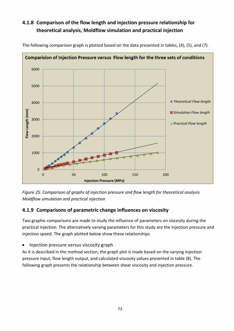
73
4.1.8 Comparison of the flow length and injection pressure relationship for
theoretical analysis, Moldflow simulation and practical injection
The following comparison graph is plotted based on the data presented in tables, (4), (5), and (7).
Figure 25. Comparison of graphs of injection pressure and flow length for theoretical analysis
Moldflow simulation and practical injection
4.1.9 Comparisons of parametric change influences on viscosity Two graphic comparisons are made to study the influence of parameters on viscosity during the
practical injection. The alternatively varying parameters for this study are the injection pressure and
injection speed. The graph plotted below show these relationships
Injection pressure versus viscosity graph
As it is described in the method section, the graph plot is made based on the varying injection
pressure input, flow length output, and calculated viscosity values presented in table (8). The
following graph presents the relationship between shear viscosity and injection pressure.
0
1000
2000
3000
4000
5000
6000
0 50 100 150 200
Flo
w L
en
gth
(m
m)
Injection Pressure (MPa)
Theoretical Flow length
Simulation Flow length
Practical Flow length
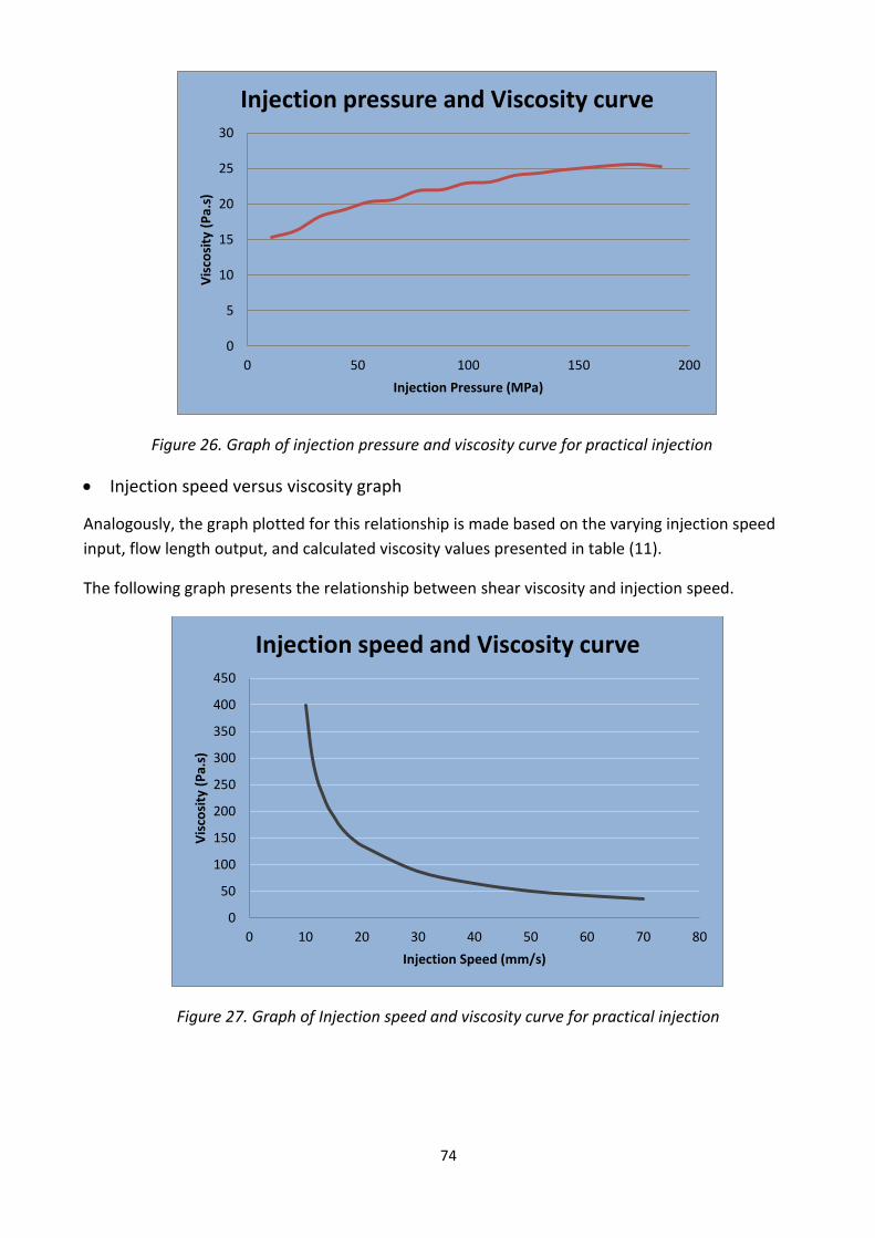
74
Figure 26. Graph of injection pressure and viscosity curve for practical injection
Injection speed versus viscosity graph
Analogously, the graph plotted for this relationship is made based on the varying injection speed
input, flow length output, and calculated viscosity values presented in table (11).
The following graph presents the relationship between shear viscosity and injection speed.
Figure 27. Graph of Injection speed and viscosity curve for practical injection
0
5
10
15
20
25
30
0 50 100 150 200
Vis
cosi
ty (
Pa.
s)
Injection Pressure (MPa)
Injection pressure and Viscosity curve
0
50
100
150
200
250
300
350
400
450
0 10 20 30 40 50 60 70 80
Vis
cosi
ty (
Pa.
s)
Injection Speed (mm/s)
Injection speed and Viscosity curve
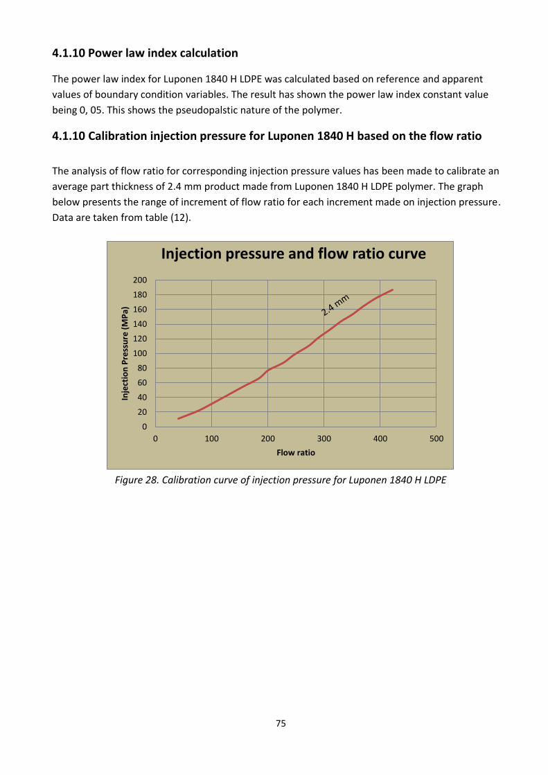
75
4.1.10 Power law index calculation
The power law index for Luponen 1840 H LDPE was calculated based on reference and apparent
values of boundary condition variables. The result has shown the power law index constant value
being 0, 05. This shows the pseudopalstic nature of the polymer.
4.1.10 Calibration injection pressure for Luponen 1840 H based on the flow ratio
The analysis of flow ratio for corresponding injection pressure values has been made to calibrate an
average part thickness of 2.4 mm product made from Luponen 1840 H LDPE polymer. The graph
below presents the range of increment of flow ratio for each increment made on injection pressure.
Data are taken from table (12).
Figure 28. Calibration curve of injection pressure for Luponen 1840 H LDPE
0
20
40
60
80
100
120
140
160
180
200
0 100 200 300 400 500
Inje
ctio
n P
ress
ure
(M
Pa)
Flow ratio
Injection pressure and flow ratio curve
76
4.2 Discussion
The thesis comprises of different discussions based on the results obtained in this part. Discussions
are made sequentially based on the steps of result findings. The results are discussed based on the
scientific findings, practical experimentations and analogous works made in the area. Isothermal flow
formula, power law index constant, and graphs of each parameter variations in theoretical,
simulation and practical outputs are discussed in this part. The discussions are made based on
comparable outputs. The following generalized terms of the result summary are discussed.
4.2.1 Isothermal flow formula
The isothermal flow formula developed for the semi-circular flow channel mathematically describes
the volume flow rate at a specified pressure level. The formula is derived based on the elemental
fluid of identical profile in the flow channel. The volume flow rate formula has been the very crucial
formula in this thesis work to analyse the viscosity values at a predefined injection pressure and
injection speed levels. The significant difference of flow channel in analysing volume flow rate
depends on the shape of the cross-section. In rectangular cross-section flow channel, as the formula
in the result shows, the height of the flow channel plays the great role in determining the flow rate.
Any change in the height of the flow channel is raised to cube to calculate the volume flow rate.
Analogously, the volume flow rate in circular or semi-circular flow channel is much influenced by the
radius. An increased change in a radius would make the volume flow rate increase with the radius
raised to power of four. However, between the flow rate of a circular and semi-circular flow
channels, there is a comparative increments as all the variables are similar. The result has presented
the volume flow rate for each shape. Mathematically, the volume flow rates of the two shapes are
related as follows:
( )
Where, , Volume flow rate of a circular cross-section (mm3/s)
, Volume flow rate of a semi-circular cross-section (mm3/s)
4.2.2 Theoretical, simulation and practical injection pressure and flow length
curves
The graph for the above three cases is plotted in the result section depicted by figure (23). The
comparison made among the three plots is based on the initial conditions and practical influences of
operation conditions. The graph indicates the theoretical injection pressure versus flow length has
much higher slope than the corresponding simulation and practical injection. The table (4) in the
method part took the initial constant viscosity values to calculate the flow length under the specified
injection pressure. The viscosity data for each of injection pressure ranges are the minimum values.
These initial viscosity data are calculated on the simulation software at a melt temperature of 220 oC
and volume flow rate of 6, 3 cm3/s. The theoretical analysis of flow length took these minimum initial
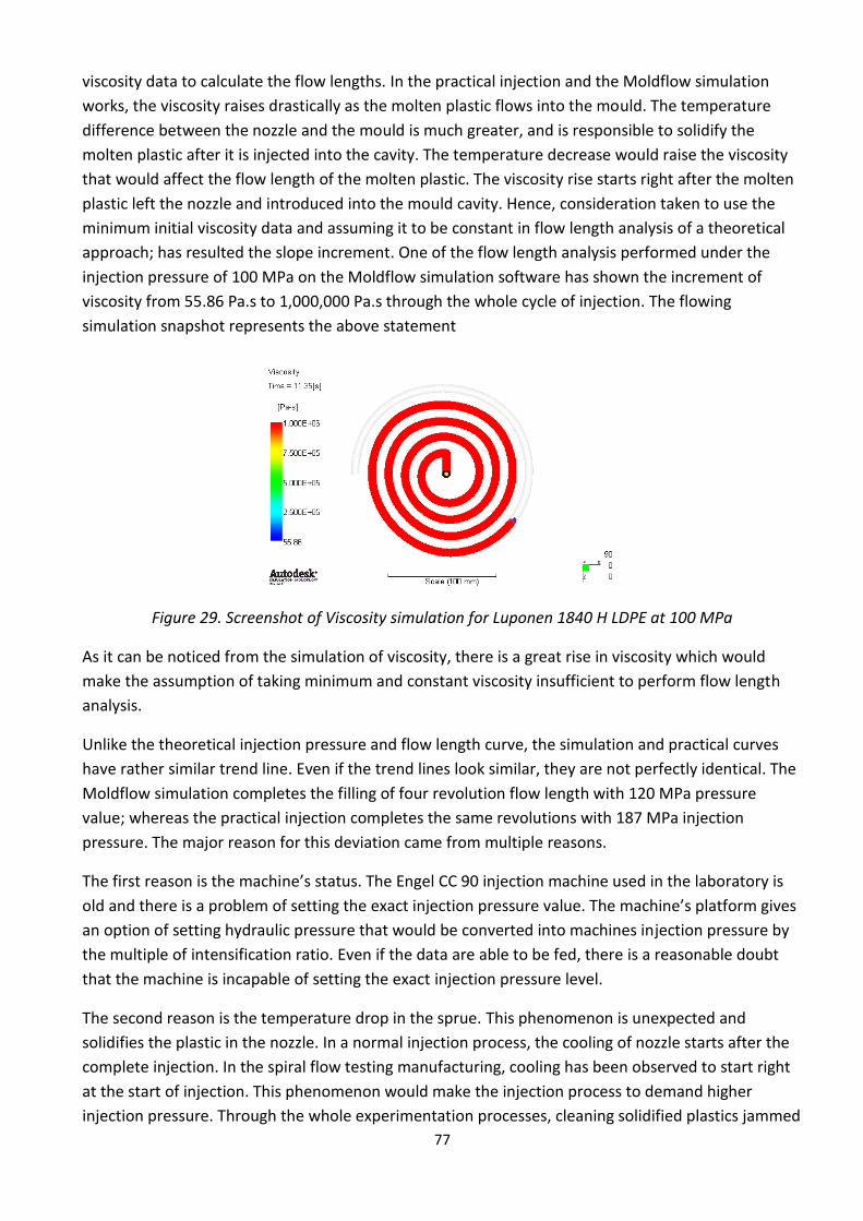
77
viscosity data to calculate the flow lengths. In the practical injection and the Moldflow simulation
works, the viscosity raises drastically as the molten plastic flows into the mould. The temperature
difference between the nozzle and the mould is much greater, and is responsible to solidify the
molten plastic after it is injected into the cavity. The temperature decrease would raise the viscosity
that would affect the flow length of the molten plastic. The viscosity rise starts right after the molten
plastic left the nozzle and introduced into the mould cavity. Hence, consideration taken to use the
minimum initial viscosity data and assuming it to be constant in flow length analysis of a theoretical
approach; has resulted the slope increment. One of the flow length analysis performed under the
injection pressure of 100 MPa on the Moldflow simulation software has shown the increment of
viscosity from 55.86 Pa.s to 1,000,000 Pa.s through the whole cycle of injection. The flowing
simulation snapshot represents the above statement
Figure 29. Screenshot of Viscosity simulation for Luponen 1840 H LDPE at 100 MPa
As it can be noticed from the simulation of viscosity, there is a great rise in viscosity which would
make the assumption of taking minimum and constant viscosity insufficient to perform flow length
analysis.
Unlike the theoretical injection pressure and flow length curve, the simulation and practical curves
have rather similar trend line. Even if the trend lines look similar, they are not perfectly identical. The
Moldflow simulation completes the filling of four revolution flow length with 120 MPa pressure
value; whereas the practical injection completes the same revolutions with 187 MPa injection
pressure. The major reason for this deviation came from multiple reasons.
The first reason is the machine’s status. The Engel CC 90 injection machine used in the laboratory is
old and there is a problem of setting the exact injection pressure value. The machine’s platform gives
an option of setting hydraulic pressure that would be converted into machines injection pressure by
the multiple of intensification ratio. Even if the data are able to be fed, there is a reasonable doubt
that the machine is incapable of setting the exact injection pressure level.
The second reason is the temperature drop in the sprue. This phenomenon is unexpected and
solidifies the plastic in the nozzle. In a normal injection process, the cooling of nozzle starts after the
complete injection. In the spiral flow testing manufacturing, cooling has been observed to start right
at the start of injection. This phenomenon would make the injection process to demand higher
injection pressure. Through the whole experimentation processes, cleaning solidified plastics jammed
78
in the sprue was done. This jamming has been blocking the molten plastic flow through the sprue,
which eventually demanded higher injection pressure.
Finally, the spure channel was ignored in calculating the flow lengths for a varying injection pressure
for the theoretical case. The sprue channel has an increasing radius all through the way from the
nozzle up to the gate of spiral. This cone shaped sprue profile makes the wall to develop both shear
and normal stresses that increase the viscosity around three times more than the shear viscosity.
Eventually the rise of viscosity in the sprue channel would contribute to the decrement of flow
length.
The above reasons have been discovered for causing the variations of injection pressures between
the simulation and actual injection processes.
4.2.3 Parametric change influences on viscosity
The influences of changes in an injection pressure and injection speed have been plotted against the
viscosity as presented in figures, (24) and (25). The curves have their own different trends which
show their relationship with viscosities. The injection pressure and injection speed relationships with
viscosity are discussed in this part of the thesis.
The injection pressure influence
As the graph in figure (24) shows in the result section, the increase in injection pressure slightly raises
the viscosity with smaller slope. This is also supported by the formula derived for the semi-circular
flow channel. The extent of the influence is determined mostly by the flow length of the
corresponding injection pressures. If the flow length was kept constant, the relationship between the
injection pressure and viscosity would be linear. The flow length variation with the corresponding
injection pressures gives the trend of the viscosities in this specific experiment. The change in
viscosity is yet observed to be closer to a constant leading to small offset of the curve from a linear
graph. Another justification for the rising viscosity with the increments injection pressure would be;
the higher the injection pressure the longer the flow length would the molten plastic flows. In order
to have a longer flow length, the fill time should be increased. However, during this lengthened fill
time, there is a temperature drop that drastically increases the viscosity. This justification strengthens
practical experimentation outputs and the viscosity analysis made based on the varying injection
pressure.
The injection speed influence
One of the fascinating results of this thesis work is to find out the behaviour of viscosity towards the
changes made in the injection speed. Many of the direct shear rates versus viscosity graphs made in
different studies quite resembles the graph plotted in this result section. The graph in figure (25),
which shows the relationship between the experimental findings of viscosity values for a varying
injection speed, resembles an inverse function with constant coefficient. This curve is quiet expected
as the flow channel has a constant cross-section all throughout. For a profile having a constant radius
all through the flow length, the graphs of viscosity versus shear rate is similar to the graph of the
79
viscosity versus injection speed. As it is implied in the literature, the shear rate and viscosity have an
inverse relationship for a constant shear stress. In the spiral flow testing, the radius is kept 3 mm for
the whole flow length, so, the behaviour of the graph is the same if the plot was made for the
viscosity versus shear rate value. The inverse relationship shown by graph also confirms the shear
thinning property of the polymer.
4.2.4 Power law index constant
The power law index constant, n, is calculated out and the result has been 0, 05. This index is less
than one that signifies the shear thinning property of the plastic. The shear thinning property of the
plastic is identified with the decrease of shear viscosity as a result of increments in shear stresses.
This constant index is quite important in determining the viscosity nature of the fluid. If the power
law index constant, n, was one, the fluid would have become ideal where the viscosity would be
constant and not affected by any parameter changes. In the last case, if n was greater than one, the
property of the fluid would be the opposite of shear thinning by increasing in viscosity for an increase
in shear stress.
The power law index constant for Luponen 1840 LDPE polymer at a specified operation conditions is
found to be 0, 05, which defines the rheological property of the polymer correctly.
4.2.5 Injection pressure calibration for Luponen 1840 H LDPE
It is quite important to determine the maximum part thickness and flow length that an injection
machine is able to produce. A good part design without manufacturability would have no meaning in
the sense of design implementation. Hence, the result section of this thesis work has calibrated the
specified average thickness of 2, 4 mm for Luponen 1840 H LDPE polymer. The calibration has helped
to determine the maximum flow ratio that can be produced without passing the pressure limit of
clamping capacity. The flow ratio has been taken as a measure of part manufacturability as it
incorporated both the length and the thickness of the part. The calibration has been made between
pressure ranges of 11 MPa and 187 MPa. The pressure increments are made constantly with the
change of 11 MPa. As it can be seen in the graph of figure (26), the plot shows a linear relationship of
injection pressure and flow ratio. The flow ratio has constantly grown with a constant increment of
injection pressure. It has been identified in this thesis that, a maximum of 187 MPa injection pressure
was used to get a flow ratio of 422 for the specified polymer. Any increment in injection pressure
above the 187 MPa has resulted in molten plastic flash through mould part line. This happened due
to the injection pressure exceeding maximum clamping capacity. It has been found out that; part
design with 2, 4 mm thickness should not exceed a flow ratio of 422 for 100 mm/s injection speed
and 187 MPa injection pressure.
80
5. CONCLUSION
The thesis includes wide range of engineering work. It includes design, analysis and manufacturing of
a spiral flow testing mould. It also formulated a spiral length, and semi-circular flow formulas to
analyse the rheological nature of a specified polymer. The formulations are made based on the basic
differential concepts of the Archimedean spiral and uniform circular flow channel. The semi-circular
flow formula has brought a fractional relationship to the common circular flow channel. Comparison
of outputs from theoretical formulation, simulation and practical injection works have been done to
give a credible scientific data and justification. The analysis implicated the maximum flow length
differences under specified injection pressures in each case. The detail analysis of injection pressure
versus flow length for Moldflow simulation showed; around four revolution or 1004, 46 mm flow
length was completed under 120 MPa injection pressure. However, for the cases of theoretical and
practical injection analyses, under the same injection pressure of 187 MPa, 1035, 5 mm and 3359, 43
mm flow lengths are observed respectively. The resulted deviations in these three cases have been
discussed in the thesis.
The thesis work breakdowns the practical injection process into pressure and speed variations to
observe the parameter influences on the viscosity of the polymer. The injection pressure curve
plotted against the viscosity has shown the general increment. However, the relationship does not
keep the linearity as the practical process is not isothermal. The temperature change influences are
observed by the non-linearity of the graph. The analysis implicated that for the range of injection
pressures 11 MPa and 187 MPa, the viscosity has shown increment from 15, 26 Pa.s up to 25, 36 Pa.s.
In addition, the inverse relationship between injection speed and viscosity, which demonstrate the
shear-thinning property of the polymer, has been observed practically. Consecutive series of injection
processes were made by increasing the injection screw speed from 10 mm/s up to 70 mm/s to
observe the corresponding viscosity decrement from 399, 23 Pa.s to 35, 63 Pa.s. Generally, analysis of
shear viscosity values at any process setup was able to be made by parameter variation. It has also
helped to observe which parameter has great influence on the viscosity nature during polymer
processing. From the above data analysed in range of values, every parameter shift has influenced
the viscosity values, but the injection speed has been observed to have the greater.
Besides, an important rheological property of the polymer under the study was characterized by
viscosity analysis. The power law shears viscosity analysis method was completely applied over the
practical injection processes to prove the polymers shear thinning property. The shear viscosity
analysis proved the shear thinning property by obtaining a power law index value of 0, 05.
Injection pressure calibration for Luponen 1840 H LDPE polymer was also made in this thesis work
using the spiral flow testing sample. The calibration would give further information on
manufacturability of new product designs made out of the same polymer. Based on this thesis, for a
maximum injection pressure of 187 MPa, the corresponding flow ratio for Luponen 1840 H LDPE of 2,
4 mm part thickness has been 422 at 100 mm/s injection speed.
Generally, the thesis has incorporated vast scope of objectives that are critically important in the
study of plastic engineering. The work has based international standards and detailed rheological

81
formulas and concepts to analyse the abstracts behind those objectives. It has completed successfully
analysing and presenting scientific explanations for each of findings.
Finally, even if the thesis work has successfully found out the power law index constant and proved
the shear thinning property of the polymer; the writer believes that the figure can be refined to
higher accuracy. In order to calculate the most accurate power law index constant, it is highly
advisable to use instruments made to measure polymers’ viscosity specifically. So, the use of
viscometer is ideal to study the viscosity data accurately.
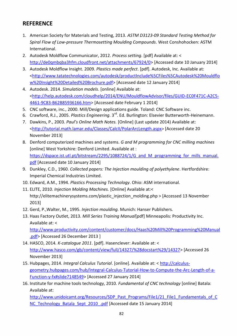
82
REFERENCE
1. American Society for Materials and Testing, 2013. ASTM D3123-09 Standard Testing Method for
Spiral Flow of Low-pressure Thermosetting Moulding Compounds. West Conshohocken: ASTM
International.
2. Autodesk Moldflow Communicator, 2012. Process setting. [pdf] Available at: <
http://de0qmbqba3hfm.cloudfront.net/attachments/67924/0> [Accessed date 10 January 2014]
3. Autodesk Moldflow Insight. 2009. Plastics made perfect. [pdf]. Autodesk, Inc. Available at:
<http://www.tatatechnologies.com/autodesk/productInclude%5CFiles%5CAutodesk%20Mouldflo
w%20Insight%20Detailed%20Brochure.pdf> [Accessed date 12 January 2014]
4. Autodesk. 2014. Simulation models. [online] Available at:
<http://help.autodesk.com/cloudhelp/2014/ENU/MouldflowAdvisor/files/GUID-EC0F471C-A2C5-
4461-9C83-B62B85936166.htm> [Accessed date February 1 2014]
5. CNC software, inc., 2000. Mill/Design applications guide. Toland: CNC Software inc. 6. Crawford, R.J., 2005. Plastics Engineering. 3rd. Ed. Burlington: Elsevier Butterworth-Heinemann.
7. Dawkins, P., 2003. Paul’s Online Math Notes. [Online] (Last update 2014) Available at:
<http://tutorial.math.lamar.edu/Classes/CalcII/PolarArcLength.aspx> [Accessed date 20
November 2013]
8. Denford computerized machines and systems. G and M programming for CNC milling machines
[online] West Yorkshire: Denford Limited. Available at :
https://dspace.ist.utl.pt/bitstream/2295/1088724/1/G_and_M_programming_for_mills_manual.
pdf [Accessed date 10 January 2014]
9. Dunkley, C.D., 1960. Collected papers: The Injection moulding of polyethylene. Hertfordshire:
Imperial Chemical Industries Limited.
10. Edward, A.M., 1994. Plastics Processing Technology. Ohio: ASM international.
11. ELITE, 2010. Injection Molding Machines. [Online] Available at:<
http://elitemachinerysystems.com/plastic_injection_molding.php > [Accessed 13 November
2013]
12. Gerd, P.,Walter, M., 1995. Injection moulding. Munich: Hanser Publishers.
13. Haas Factory Outlet, 2013. Mill Series Training Manual[pdf] Minneapolis: Productivity Inc.
Available at: <
http://www.productivity.com/content/customer/docs/Haas%20Mill%20Programming%20Manual
.pdf> [Accessed 26 December 2013 ]
14. HASCO, 2014. K-catalogue 2011. [pdf]. Hasenclever: Available at: <
http://www.hasco.com/gb/content/view/full/14327/%28docstart%29/14327> [Accessed 26
November 2013]
15. Hubpages, 2014. Integral Calculus Tutorial. [online]. Available at: < http://calculus-
geometry.hubpages.com/hub/Integral-Calculus-Tutorial-How-to-Compute-the-Arc-Length-of-a-
Function-y-fx#slide7148549> [Accessed 27 January 2014]
16. Institute for machine tools technology, 2010. Fundamental of CNC technology [online] Batala:
Available at:
http://www.unidoicamt.org/Resources/SDP_Past_Programs/File1/21_File1_Fundamentals_of_C
NC_Technology_Batala_Sept_2010_.pdf [Accessed date 15 January 2014]
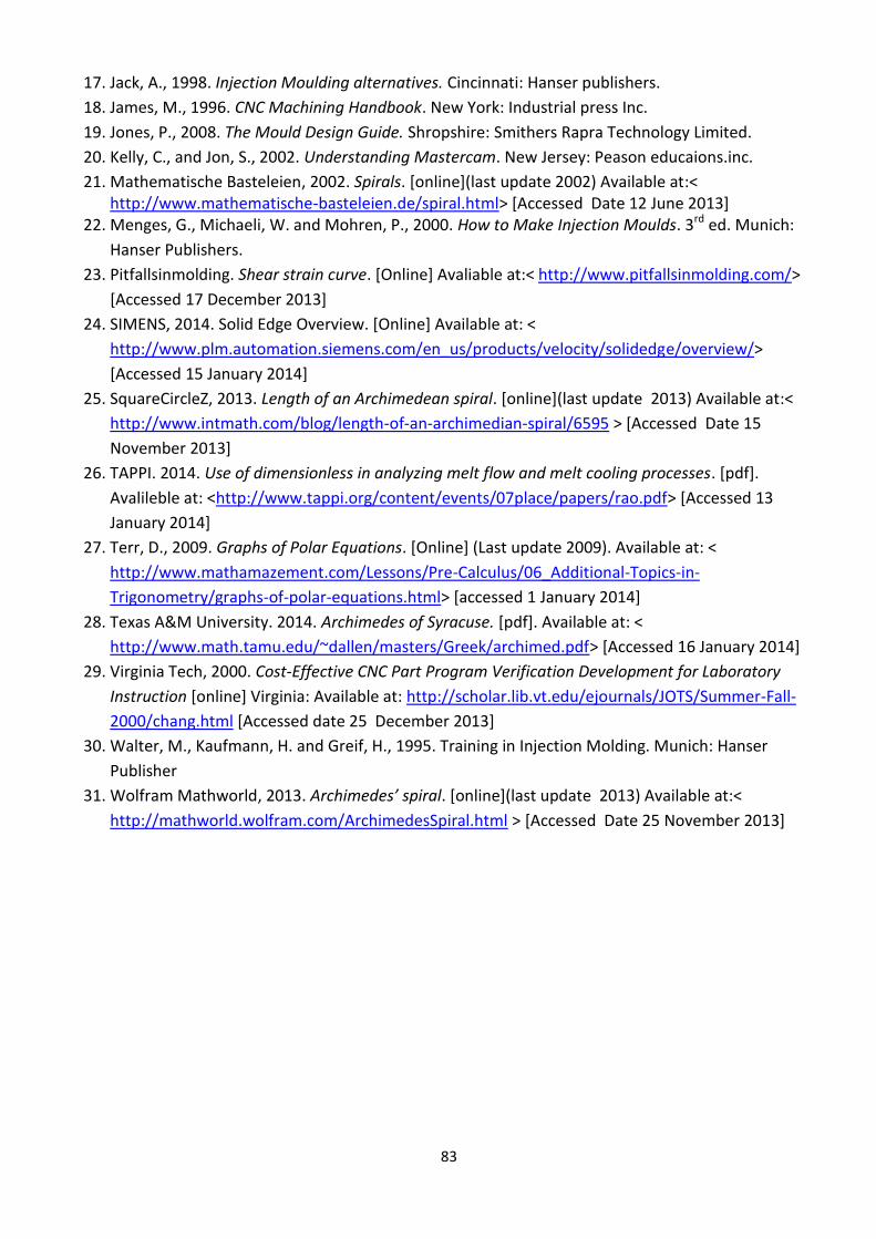
83
17. Jack, A., 1998. Injection Moulding alternatives. Cincinnati: Hanser publishers.
18. James, M., 1996. CNC Machining Handbook. New York: Industrial press Inc.
19. Jones, P., 2008. The Mould Design Guide. Shropshire: Smithers Rapra Technology Limited.
20. Kelly, C., and Jon, S., 2002. Understanding Mastercam. New Jersey: Peason educaions.inc.
21. Mathematische Basteleien, 2002. Spirals. [online](last update 2002) Available at:< http://www.mathematische-basteleien.de/spiral.html> [Accessed Date 12 June 2013]
22. Menges, G., Michaeli, W. and Mohren, P., 2000. How to Make Injection Moulds. 3rd ed. Munich:
Hanser Publishers.
23. Pitfallsinmolding. Shear strain curve. [Online] Avaliable at:< http://www.pitfallsinmolding.com/>
[Accessed 17 December 2013]
24. SIMENS, 2014. Solid Edge Overview. [Online] Available at: <
http://www.plm.automation.siemens.com/en_us/products/velocity/solidedge/overview/>
[Accessed 15 January 2014]
25. SquareCircleZ, 2013. Length of an Archimedean spiral. [online](last update 2013) Available at:<
http://www.intmath.com/blog/length-of-an-archimedian-spiral/6595 > [Accessed Date 15
November 2013]
26. TAPPI. 2014. Use of dimensionless in analyzing melt flow and melt cooling processes. [pdf].
Avalileble at: <http://www.tappi.org/content/events/07place/papers/rao.pdf> [Accessed 13
January 2014]
27. Terr, D., 2009. Graphs of Polar Equations. [Online] (Last update 2009). Available at: <
http://www.mathamazement.com/Lessons/Pre-Calculus/06_Additional-Topics-in-
Trigonometry/graphs-of-polar-equations.html> [accessed 1 January 2014]
28. Texas A&M University. 2014. Archimedes of Syracuse. [pdf]. Available at: <
http://www.math.tamu.edu/~dallen/masters/Greek/archimed.pdf> [Accessed 16 January 2014]
29. Virginia Tech, 2000. Cost-Effective CNC Part Program Verification Development for Laboratory
Instruction [online] Virginia: Available at: http://scholar.lib.vt.edu/ejournals/JOTS/Summer-Fall-
2000/chang.html [Accessed date 25 December 2013]
30. Walter, M., Kaufmann, H. and Greif, H., 1995. Training in Injection Molding. Munich: Hanser
Publisher
31. Wolfram Mathworld, 2013. Archimedes’ spiral. [online](last update 2013) Available at:<
http://mathworld.wolfram.com/ArchimedesSpiral.html > [Accessed Date 25 November 2013]
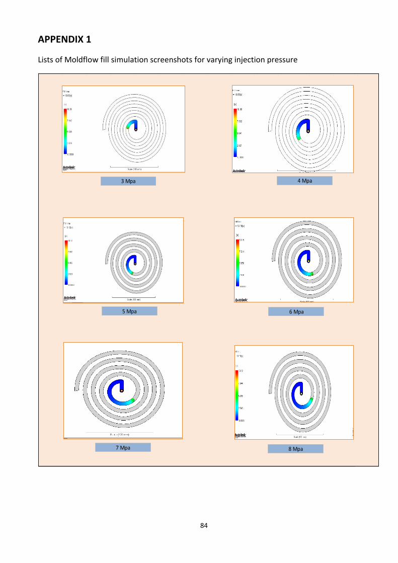
84
APPENDIX 1
Lists of Moldflow fill simulation screenshots for varying injection pressure
3 Mpa 4 Mpa
5 Mpa 6 Mpa
7 Mpa 8 Mpa
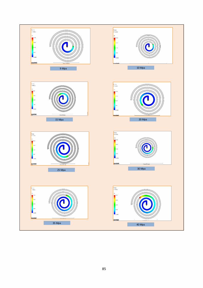
85
9 Mpa 10 Mpa
15 Mpa 20 Mpa
25 Mpa 30 Mpa
35 Mpa40 Mpa
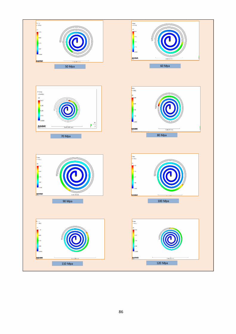
86
50 Mpa 60 Mpa
70 Mpa 80 Mpa
90 Mpa 100 Mpa
110 Mpa 120 Mpa

87
APPENDIX 2
Set up sheet for mould cavity mill simulation on Mastercam
CUSTOMIZABLE MILL SETUP SHEET - MILL.SET
=========================================
PROGRAM NAME = CAVITY_MILL
DATE PROCESSED = MAR. 14 2014
TIME = 12:15 PM
MATERIAL TYPE = ALUMINUM mm - 2024
STOCK SIZE = X156.000 Y156.000 Z28.000
STOCK ORIGIN = X0. Y0. Z0.(AT CENTER, Z AT TOP)
MACHINE NAME = GENERIC MILL
GROUP NAME = MACHINE GROUP-1
--------------------------------------------------------------
OPERATION TYPE = DRILL CYCLE - PECK
TOOL NAME = 3/8 CENTER DRILL
TOOL DEF. (MANUFACTURER) =
TOOL DEF. (CHUCK) =
TOOL NUM. = 12
TOOL DIA. = .375
DRILL TIP ANGLE = 90.
FLUTE LEN. = 50.
OVERALL LEN. = 75.
SHOULDER LEN. = 60.
ARBOR DIA. = 5.
HOLDER DIA. = 50.
DIA. OFFSET = 12
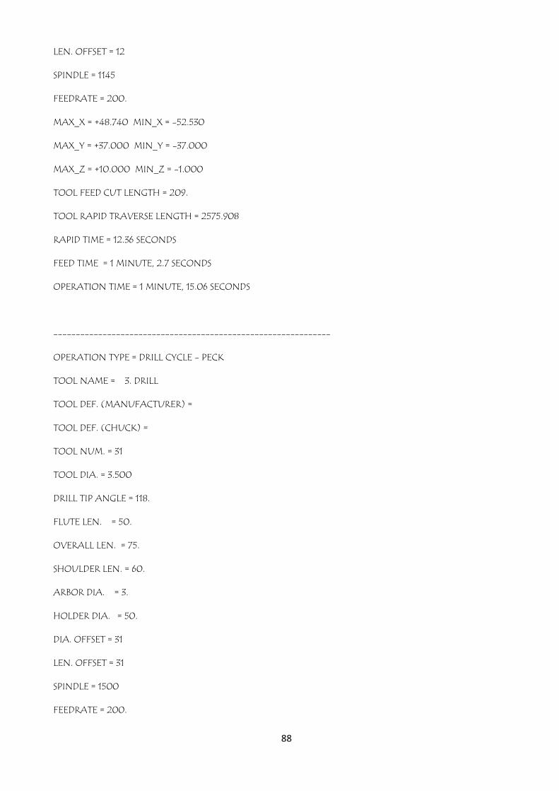
88
LEN. OFFSET = 12
SPINDLE = 1145
FEEDRATE = 200.
MAX_X = +48.740 MIN_X = -52.530
MAX_Y = +37.000 MIN_Y = -37.000
MAX_Z = +10.000 MIN_Z = -1.000
TOOL FEED CUT LENGTH = 209.
TOOL RAPID TRAVERSE LENGTH = 2575.908
RAPID TIME = 12.36 SECONDS
FEED TIME = 1 MINUTE, 2.7 SECONDS
OPERATION TIME = 1 MINUTE, 15.06 SECONDS
--------------------------------------------------------------
OPERATION TYPE = DRILL CYCLE - PECK
TOOL NAME = 3. DRILL
TOOL DEF. (MANUFACTURER) =
TOOL DEF. (CHUCK) =
TOOL NUM. = 31
TOOL DIA. = 3.500
DRILL TIP ANGLE = 118.
FLUTE LEN. = 50.
OVERALL LEN. = 75.
SHOULDER LEN. = 60.
ARBOR DIA. = 3.
HOLDER DIA. = 50.
DIA. OFFSET = 31
LEN. OFFSET = 31
SPINDLE = 1500
FEEDRATE = 200.
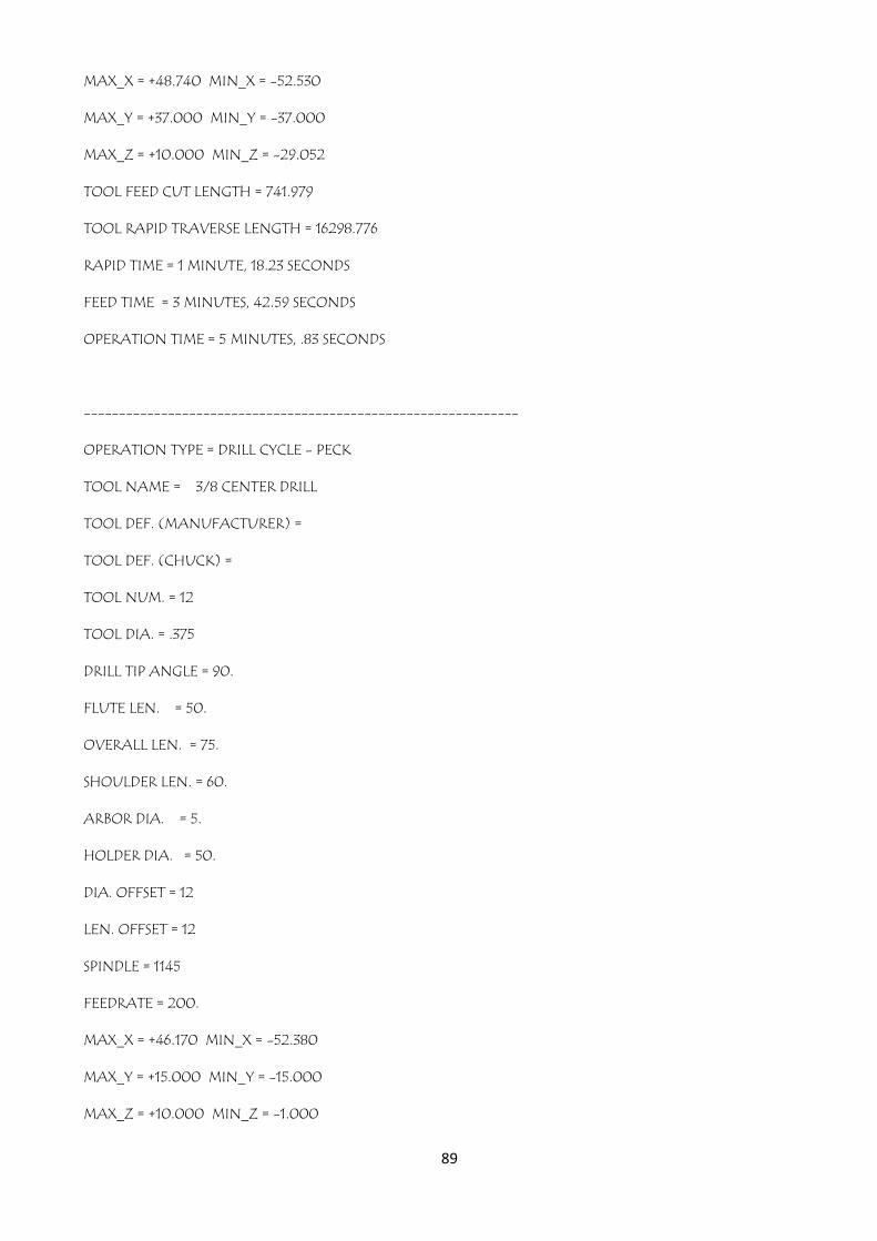
89
MAX_X = +48.740 MIN_X = -52.530
MAX_Y = +37.000 MIN_Y = -37.000
MAX_Z = +10.000 MIN_Z = -29.052
TOOL FEED CUT LENGTH = 741.979
TOOL RAPID TRAVERSE LENGTH = 16298.776
RAPID TIME = 1 MINUTE, 18.23 SECONDS
FEED TIME = 3 MINUTES, 42.59 SECONDS
OPERATION TIME = 5 MINUTES, .83 SECONDS
--------------------------------------------------------------
OPERATION TYPE = DRILL CYCLE - PECK
TOOL NAME = 3/8 CENTER DRILL
TOOL DEF. (MANUFACTURER) =
TOOL DEF. (CHUCK) =
TOOL NUM. = 12
TOOL DIA. = .375
DRILL TIP ANGLE = 90.
FLUTE LEN. = 50.
OVERALL LEN. = 75.
SHOULDER LEN. = 60.
ARBOR DIA. = 5.
HOLDER DIA. = 50.
DIA. OFFSET = 12
LEN. OFFSET = 12
SPINDLE = 1145
FEEDRATE = 200.
MAX_X = +46.170 MIN_X = -52.380
MAX_Y = +15.000 MIN_Y = -15.000
MAX_Z = +10.000 MIN_Z = -1.000
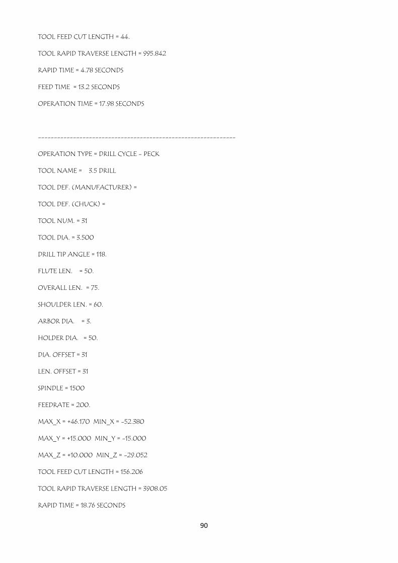
90
TOOL FEED CUT LENGTH = 44.
TOOL RAPID TRAVERSE LENGTH = 995.842
RAPID TIME = 4.78 SECONDS
FEED TIME = 13.2 SECONDS
OPERATION TIME = 17.98 SECONDS
--------------------------------------------------------------
OPERATION TYPE = DRILL CYCLE - PECK
TOOL NAME = 3.5 DRILL
TOOL DEF. (MANUFACTURER) =
TOOL DEF. (CHUCK) =
TOOL NUM. = 31
TOOL DIA. = 3.500
DRILL TIP ANGLE = 118.
FLUTE LEN. = 50.
OVERALL LEN. = 75.
SHOULDER LEN. = 60.
ARBOR DIA. = 3.
HOLDER DIA. = 50.
DIA. OFFSET = 31
LEN. OFFSET = 31
SPINDLE = 1500
FEEDRATE = 200.
MAX_X = +46.170 MIN_X = -52.380
MAX_Y = +15.000 MIN_Y = -15.000
MAX_Z = +10.000 MIN_Z = -29.052
TOOL FEED CUT LENGTH = 156.206
TOOL RAPID TRAVERSE LENGTH = 3908.05
RAPID TIME = 18.76 SECONDS

91
FEED TIME = 46.86 SECONDS
OPERATION TIME = 1 MINUTE, 5.62 SECONDS
--------------------------------------------------------------
OPERATION TYPE = DRILL CYCLE - PECK
TOOL NAME = 12. DRILL
TOOL DEF. (MANUFACTURER) =
TOOL DEF. (CHUCK) =
TOOL NUM. = 48
TOOL DIA. = 12.000
DRILL TIP ANGLE = 118.
FLUTE LEN. = 50.
OVERALL LEN. = 75.
SHOULDER LEN. = 60.
ARBOR DIA. = 12.
HOLDER DIA. = 50.
DIA. OFFSET = 48
LEN. OFFSET = 48
SPINDLE = 1000
FEEDRATE = 300.
FEEDRATES: MAX = 300. MIN = 300.
MAX_X = +0.000 MIN_X = +0.000
MAX_Y = +0.000 MIN_Y = +0.000
MAX_Z = +10.000 MIN_Z = -33.000
TOOL FEED CUT LENGTH = 43.
TOOL RAPID TRAVERSE LENGTH = 1560.553
RAPID TIME = 7.49 SECONDS
FEED TIME = 8.6 SECONDS
OPERATION TIME = 16.09 SECONDS
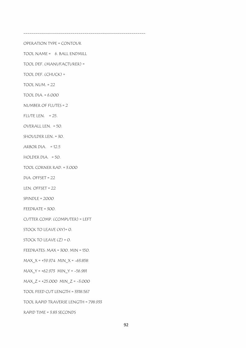
92
--------------------------------------------------------------
OPERATION TYPE = CONTOUR
TOOL NAME = 6. BALL ENDMILL
TOOL DEF. (MANUFACTURER) =
TOOL DEF. (CHUCK) =
TOOL NUM. = 22
TOOL DIA. = 6.000
NUMBER OF FLUTES = 2
FLUTE LEN. = 25.
OVERALL LEN. = 50.
SHOULDER LEN. = 30.
ARBOR DIA. = 12.5
HOLDER DIA. = 50.
TOOL CORNER RAD. = 3.000
DIA. OFFSET = 22
LEN. OFFSET = 22
SPINDLE = 2000
FEEDRATE = 300.
CUTTER COMP. (COMPUTER) = LEFT
STOCK TO LEAVE (XY)= 0.
STOCK TO LEAVE (Z) = 0.
FEEDRATES: MAX = 300. MIN = 150.
MAX_X = +59.974 MIN_X = -63.858
MAX_Y = +62.973 MIN_Y = -56.981
MAX_Z = +25.000 MIN_Z = -3.000
TOOL FEED CUT LENGTH = 3318.567
TOOL RAPID TRAVERSE LENGTH = 798.933
RAPID TIME = 3.83 SECONDS

93
FEED TIME = 11 MINUTES, 15.31 SECONDS
OPERATION TIME = 11 MINUTES, 19.15 SECONDS
==============================================================
PROGRAM TOTALS (6 TOOLS):
FEEDRATES: MAX = 300. MIN = 150.
MAX_X = +59.974 MIN_X = -63.858
MAX_Y = +62.973 MIN_Y = -56.981
MAX_Z = +25.000 MIN_Z = -33.000
TOTAL FEED CUT LENGTH = 4512.752
TOTAL RAPID TRAVERSE LENGTH = 26138.062
TOTAL RAPID TIME = 2 MINUTES, 5.46 SECONDS
TOTAL FEED TIME = 17 MINUTES, 9.27 SECONDS
CYCLE TIME: 19 MINUTES, 50.73 SECONDS

94