Manufacturing Cost Flow Diagrams as an Alternative Method ... · PDF fileload theory in accounting education research.” ... visually-based diagrams in the classroom over a decade

Manufacturing Cost Flow Diagrams as an Alternative Method of External Problem Representation - A Diagrammatic Approach to Teaching Cost

Accounting and Evidence of Its Effectiveness

Katherine J. Silvester Siena College

John C. O’Neill Siena College

This paper introduces a new visually-based diagrammatic pedagogical approach that utilizes manufacturing cost flow diagrams as an alternative method of external problem representation. Statistical and graphical analysis of test scores indicate a significant improvement in the performance of undergraduate accounting students when this diagrammatic pedagogical approach is utilized. These results are consistent with previous findings in the cognitive science literature that the use of diagrams may allow students to process relationships and complex data in chunks, thereby processing more effectively. INTRODUCTION

Undergraduate accounting students can have a difficult time conceptualizing manufacturing processes, their physical inventory flows, and the accompanying accounting cost flows. Traditional methods of teaching this material within the management and cost accounting classes heavily stress the memorization of the transactional and reporting requirements. Such approaches frequently focus on the detailed cost calculations, journal entries, general ledger “T” accounts, as well as the resulting GAAP and inventory reports. As a result of this large amount of minutia and inherent complexity, students may fail to make the conceptual linkages necessary for a solid foundational understanding of the processes (both physical flows and cost flows) involved in manufacturing accounting. Graphical and visual diagrams, when utilized, are very elementary and relatively undeveloped. Due to their lack of understanding, students may also come to view the various topics in a typical cost accounting or managerial accounting course as unrelated and disjointed. Others have noted these difficulties and have proposed various ways (pedagogical, conceptual, and/or strategic) of addressing the issue (Greenberg and Wilner, 2011; Blocher, 2009).

This paper presents an extensive and detailed diagrammatic approach that can help accounting students develop an innate understanding of inventory and cost flows across multiple cost accounting topics. We theorize that when this manufacturing cost flow diagram and representation method is utilized, students may be better able to organize and analyze complex situations by cognitively processing the individual process components as chunks of data (Mayer, 1976). As a result, students may then be able to discern the inter-relatedness of topics that they previously viewed as unrelated and disjointed.

Journal of Higher Education Theory and Practice Vol. 16(2) 2016 81

The remainder of this paper is organized as follows. The first section discusses problem representation from the perspective of the cognitive science literature. We also present our manufacturing diagrammatic approach to external problem representation in inventory and cost accounting. We include specific diagrammatic solutions to three types of cost accounting problems. The second section discusses the measurement and assessment of student performance and potential confounding variables in an undergraduate classroom setting. The third section contains the statistical analysis of student achievement of learning objectives and the related discussion. This section also includes both numerical and graphical evidence that a significant improvement in student performance is associated with our diagrammatic approach to external problem representation in manufacturing cost accounting. In the final sections, we discuss the limitations of our study and the potential application of diagrammatic problem representation to other areas in accounting. EXTERNAL PROBLEM REPRESENTATION Cognitive Theory and Problem Representation

Early academic work in cognitive theory supports the value of visual cognitive tools in problem representation and in learning. Schwartz (1971) found that the use of visual cognitive tools (diagrammatic representations such as matrices, graphs, and visual grouping) led to better student performance in problem solving than verbal representations (sentences) alone. Mayer (1976; 1989) found that visual (spatial) representations of problems can be particularly useful when the amount of detail and complexity is high. When Mayer compared verbal and flow diagram problem representation formats, while controlling for four different levels of problem complexity, he found that student performance in solving the problems was significantly higher when the flow diagram format was used with more complex problems. In the more complex problems, he hypothesized that students were probably not able to comprehend the overall structure of the problem as a single “chunk” of information. He theorized that the diagrammatic representation of the problem may have helped students to integrate complex information into an understandable structure or “chunk.” Thus, well-structured problem representations (such as flow diagrams) may allow a student to integrate and utilize larger chunks of information into limited working memory. Larkin and Simon (1987) theorized that diagrams grouped information together so that the user did not have to expend as much effort in cognitive activities, such as search, matching, and perceptual inference. Correspondingly, Jones and Schkade (1995, p. 215) noted that “alternative representations, even if they are informationally equivalent, can differ in the demands they place on the decision makers’ cognitive abilities.” Therefore, the benefit of such alternative external problem representations does not depend upon whether they offer additional information to the learner. The benefit of alternative external representations lies in their potential to reduce the cognitive load on the learner. Mostyn (2012, p. 241) further discussed the application of cognitive load theory and “chunking” specifically to accounting pedagogy, while noting that there “does not appear to be a widespread awareness or inclusion of cognitive load theory in accounting education research.” This paper specifically addresses this lack of awareness and inclusion in accounting education.

Initially intrigued by the potential value of using alternative problem representations, such as flow diagrams, to aid students in processing and learning, we began experimenting with expansions of visually-based diagrams in the classroom over a decade ago. Correspondingly, past and current work in cognitive load theory provides theoretical support for the potential benefits of such an approach. Diagrammatic External Problem Representation in Cost Accounting Manufacturing Cost Flow Diagramming

When we first began teaching cost and manufacturing accounting, we noticed that many students approached product costing from a relatively formulaic perspective – memorizing formulas, definitions, and journal entries. To aid students in moving to a deeper understanding of the material, we began to develop and present flow diagrams of the processes involved in manufacturing product costing. Initially, we applied the principles of spatial representation and visualization by introducing and adapting the

82 Journal of Higher Education Theory and Practice Vol. 16(2) 2016

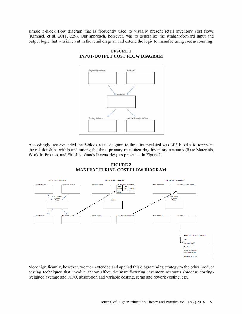
simple 5-block flow diagram that is frequently used to visually present retail inventory cost flows (Kimmel, et al. 2011, 229). Our approach, however, was to generalize the straight-forward input and output logic that was inherent in the retail diagram and extend the logic to manufacturing cost accounting.

FIGURE 1 INPUT-OUTPUT COST FLOW DIAGRAM

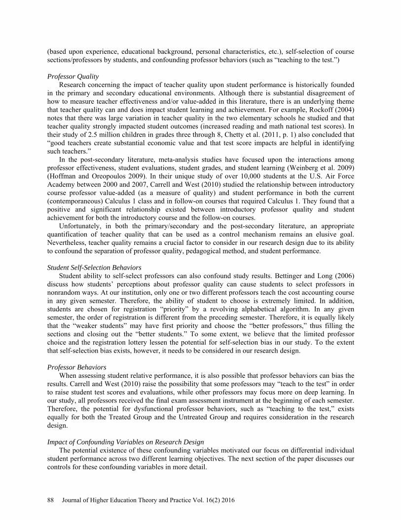
Accordingly, we expanded the 5-block retail diagram to three inter-related sets of 5 blocks1 to represent the relationships within and among the three primary manufacturing inventory accounts (Raw Materials, Work-in-Process, and Finished Goods Inventories), as presented in Figure 2.

FIGURE 2 MANUFACTURING COST FLOW DIAGRAM

More significantly, however, we then extended and applied this diagramming strategy to the other product costing techniques that involve and/or affect the manufacturing inventory accounts (process costing- weighted average and FIFO, absorption and variable costing, scrap and rework costing, etc.).


We found the use of manufacturing cost flow diagramming to be a particularly useful visualization and external representation tool in the cost accounting course because it allowed students to follow the flow of products and costs through and within the manufacturing inventory accounts in a very structured and analytical manner. The manufacturing cost flow diagram approach also provided a foundation for the student to move from memorization to understanding the dynamic meaning behind the static formulas for various computations. Anecdotally, it seemed that the application of diagramming to many of the other topics in cost accounting led to significant gains in student engagement, learning, and retention of the material.

As mentioned previously, Figure 2 presents the manufacturing cost flow diagram used in modeling a detailed Multi-Step Income Statement for Manufacturers. The structure highlights the iterative patterns that underlie the calculations for Cost of Goods Sold, Cost of Goods Manufactured, Material Purchases, Materials Used, and the other intermediary components of manufacturing accounting. The diagram provides the student with a visual model that he can use to move to the analysis level of learning.

We believe that the key to deepening student learning in cost accounting is in leading the students to visualize the relationships among the data, before students move on to preparing the formal statements. Our use of the manufacturing cost flow diagram approach leads accounting students towards a view of business operations as inter-related processes and activities. By diagramming, students naturally begin to analyze cost flows and processes by visualizing the process components, flows, and linkages and then comparing and contrasting them. This is the essence of Bloom’s (1956, p. 144) definition of analysis: “Analysis emphasizes the breakdown of the material into its constituent parts and detection of the relationships of the parts and of the way they are organized.” Developing the students’ abilities to understand and to analyze represent higher levels of learning in Bloom’s Taxonomy of Educational Objectives (1956) than memorization alone.2

In order to demonstrate the use of the manufacturing cost flow diagramming approach, we have included a sample of three illustrative problems in Appendices 1, 2, and 3. A description of these problems is presented below.

Diagramming the Manufacturer’s Multi-Step Income Statement and Balance Sheet Accounts

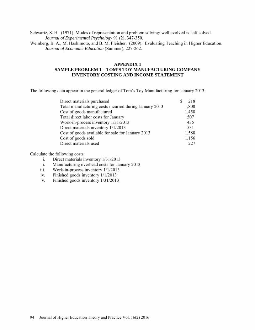
To contrast the standard and the diagrammatic methods, Appendix 1 contains a typical multi-step manufacturing inventory problem (Tom’s Toy Manufacturing Company), along with its standard solution. The standard solution requires the student to recall the formulas that are imbedded in the Multi-Step Income Statement in order to calculate the various missing items. For many students, this becomes simply a rote memorization task – which represents the lowest level of learning (Knowledge) in Bloom’s Taxonomy (1956).

We next present the corresponding manufacturing cost flow diagram used for visualizing and then analyzing inventory cost flows and the associated “T” account details. Utilizing the diagrammatic approach, students begin the process by first recalling the logical flow of costs (as seen in the cost flow diagram), and then linking the specific names of each “box” under each type of inventory. In this process, students recognize the pattern of the manufacturing cost flows. For example, additions to the Direct Materials Inventory are “Purchases of Materials”, while additions to the Work-in-Process Inventory are “Manufacturing Cost Incurred”, and additions to the Finished Goods Inventory are “Cost of Goods Manufactured”. The cost flow diagram enables students to explicitly and easily recognize and utilize the relationships and patterns within the inventory accounts, when solving the problem.3 Pedagogically, students can then be shown that by understanding the components in the manufacturing cost flow diagram, they have already memorized the logic, structure, and patterns embedded in the detailed Multi-Step Income Statement and the associated Balance Sheet general ledger accounts. To emphasize this point, we generally require students to also produce the relevant “T” account details. Diagramming Process Costing Problems (Work-in-Process Inventories)

A detailed example of applying the manufacturing cost flow diagram approach to a more complex product costing topic that involves the Work-in-Process Inventories is shown in Appendix 2. This


example includes a weighted average process costing problem (Chrome Watch Company), a standard production report solution, our cost flow diagrammatic solution, and the associated journal entry. When utilizing the standard approach, we have repeatedly observed the difficulty that students experience in trying to memorize, understand, and create the production report. Anecdotally, students generally find the production report format and logic confusing and non-intuitive.

To solve the process costing problem using the diagrammatic approach, the student first constructs the 5-block manufacturing cost flow diagram that represents the Work-in-Process Inventory account of Chrome’s Inspection Department. The student completes the flow diagram structure by including the details within each component of the Inspection Department Work-in-Process Inventory account (i.e., physical units, percent of completion, and equivalent units for the ending balance). In the next step, the student calculates the weighted average cost rate per equivalent unit of production and assigns costs to the ending balance and to the units transferred out to the Packaging Department Work-in-Process account. Finally, the student constructs the journal entry to record the transfer of the cost of the completed units to the Packaging Department Work-in-Process account.

The diagrammatic approach to solving process costing problems stresses analyzing the physical flows and the corresponding data flows, rather than the completion of the standard production report that is typically generated when teaching process costing. The diagrammatic method leads naturally to the recording of the appropriate journal entries to record production activities, since each journal entry is uniquely identified with a line or component in the flow diagram, as indicated in Appendix 2. The cost flow diagram approach is also easily adapted to handle FIFO process costing, as well as including the costing of rejects, rework, and waste when calculating and recording these manufacturing outputs. We typically include these topics in our Advanced Cost Accounting class, with their associated diagrams. Diagramming Absorption and Variable Costing Problems (Finished Goods Inventories)

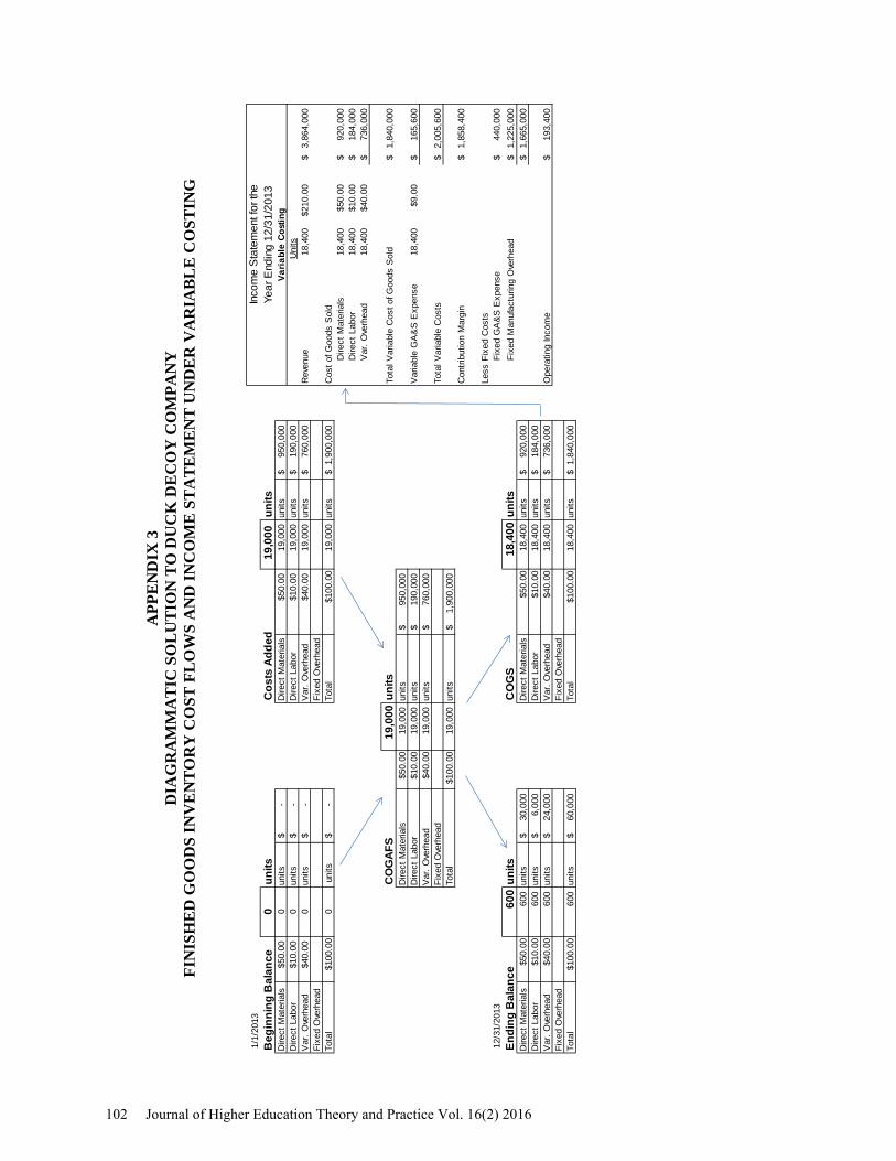
We also use the diagrammatic approach to help students understand and reconcile the differences between absorption and variable costing and the cost flows through the Finished Goods Inventory, as well as the resulting income statements. Appendix 3 includes a typical first-year absorption and variable costing problem (Duck Decoy Company), a standard solution, and our cost flow diagrammatic solution.

In this problem, the manufacturing cost flow diagram focuses upon the Finished Goods Inventory and illuminates the differential flow of fixed costs to the Income Statement. By diagramming the cost flows in this example, students can easily recognize three important points regarding the different approaches to costing. First, it is clear that fixed overhead costs flow through the inventory accounts in absorption costing, while fixed overhead costs are not included (equal zero) in the inventory accounts in variable costing. (See the Fixed Overhead line item in the Costs Added box on the flow diagrams in Appendix 3.) Second, the $36,750 difference in Net Income between the variable and absorption income statements ($230,150 - $193,400) is easily identified within the ending balance of the Finished Goods Inventory. (See the Fixed Overhead line item for 600 units @ $61.25 per unit = $36,750 on the absorption costing diagram). Third, the calculation of the production volume variance is straight-forward since the fixed cost per unit rate is explicitly identified in the flow diagram ($61.25 x 1,000 units = $61,250).

This application of the manufacturing cost flow diagram approach is especially useful in multi-year situations where multiple layers of overhead costs occur. In multi-year situations, students can visually view and trace the changes in the ending balance of Finished Goods from the previous year to the current year in order to reconcile the differences in the current year Income Statements. Thus, the diagrammatic external problem diagrams allow the student to easily visualize, identify, and understand these differences. Student Reaction to the Diagrammatic Approach Anecdotal Evidence

Anecdotally, students have historically expressed a very positive reaction to using the cost flow diagram approach within the cost accounting course. At accounting events, our alumni have regularly referred to the cost flow diagram as one of the more useful and generalizable tools they learned in


accounting. Many graduates have told us their stories about analyzing CPA exam questions (both cost and financial) by diagramming the problems. This feedback, as well as our observations and experiences in the classroom, have led to our continued use of the diagrammatic approach. Empirical Evidence

Empirically, however, the question remained as to whether our use of visually-based manufacturing cost flow diagrams for external problem representation was associated with a demonstrable improvement in student learning and performance. Student enthusiasm and extensive use of the method, while gratifying, did not necessarily imply a measurable improvement in learning or performance. Specifically, we wondered, is the use of the cost flow diagram method in teaching product costing topics associated with improved student performance and achievement of our course product costing learning objective?

To address this question, we turned to the historical data from our formal institutional assessment reports to study the relative performance of students taught using the cost flow diagram method (Treated Group) compared to the performance of students taught using traditional methods (Untreated Group). Examining this question in detail, however, raised the challenge of assessing student performance in the presence of potential confounding variables, such as professor quality, student self-selection bias, and professor behaviors.

Obviously, pedagogical studies such as this do not conform to a classical experimental design, however, analyzing those results provide insight into that which is effective in its delivery. MEASURING AND ASSESSING STUDENT PERFORMANCE Existing Institutional Assessment Procedures

Our institution is accredited by the Middle States Commission on Higher Education. In addition, our School of Business is also accredited by the Association to Advance Collegiate Schools of Business (AACSB). As an accredited institution, our School of Business utilizes a pre-established assessment procedure for measurement of student attainment of learning objectives at the course, certificate, degree, and school level. Throughout the School of Business, multiple sections of each major course are coordinated through the use of a common course guide. The common course guide serves as the basis for coordinating syllabi from different faculty teaching the same course across different semesters. This approach ensures that all sections of each course are consistent in terms of the subject matter coverage, textbook, common final exam, and assessment of the attainment of learning objectives for quality improvement efforts. The course guide approach also allows for significant faculty academic freedom within sections as to teaching methodology, as well as design and grading of assignments, course exams, etc.

Our B.S. in Accounting requires the successful completion of a standard junior level 3-credit hour cost accounting course. For assessment purposes, the cost accounting course is divided into four major areas, each associated with its own separate learning objective, as specified in Table 1. The course guide for the cost accounting course requires a common, comprehensive final exam each semester for assessment of individual student performance against our pre-established Learning Objectives 2, 3 and 4 across all sections of the course. (Learning Objective 1 on Ethics is evaluated via a separate individual student case analysis and writing assignment.)


TABLE 1 LEARNING OBJECTIVES FOR THE COST ACCOUNTING COURSE

L.O. #

Learning Objective Name

Description from Course Guide and Syllabus

Assessment Instrument

1 Ethics

Examine a business situation, apply the Institute of Management Accountants Code of Ethics, and formulate an acceptable course of action

Student Case Analysis

2 Cost Estimation Analyze historical data in order to estimate costs for future management decision making

7-9 Final Exam Questions

3 Product Costing Calculate appropriate product costs within a designated business environment

16 Final Exam Questions

4 Variance Analysis Prepare and interpret budgets and operating results through variance analysis

12 Final Exam Questions

Final Exam Assessment Instrument

The course final exam is a required, common, multiple-choice, cumulative and comprehensive exam for the course. To ensure student effort, the final exam is also a significant portion of each student’s overall course grade. The final exam is comprised of 40 questions that address the technical content of the course.4 All professors teaching the cost accounting course receive a copy of the final exam at the beginning of each semester. The final exam is a closely-guarded instrument, and accordingly, the specific final exam questions are not available to students outside of the final exam test period. Of the 40 questions on the final exam, 37 questions are used for assessment of course learning objectives. Students are asked 9 questions about Cost Estimation (Learning Objective 2), 16 questions about Product Costing (Learning Objective 3), and 12 questions about Variance Analysis (Learning Objective 4). Although it is presented in a multiple-choice format, the exam stresses calculation, application of theory, and analysis.

35 of the core 37 assessment questions have remained essentially unchanged during the three-year period of study. (Only minor grammatical and/or clarification changes were made to these basic 35 questions.) However, effective Spring 2010, two questions regarding an old learning objective were dropped and two questions were added to the section of the final exam addressing Learning Objective 2. Therefore, the number of questions used to assess Learning Objective 2 increased from 7 to 9 beginning that semester, while the total number of assessment questions remained at 37. (This change in Learning Objective 2 impacted our research design, as discussed later in the paper.)

During the six semesters in our study, there were no substantive changes to the final exam with respect to Learning Objectives 3 or 4. This stability in both the number and content of the final exam questions for these two learning objectives over time offers a unique opportunity to study the performance of many students across multiple semesters and multiple professors.

Specifically, this paper utilizes and analyzes the common final exam assessment data in order to study the impact of the manufacturing cost flow diagram teaching methodology on student achievement on Learning Objective 3–Product Costing. Potential Confounding Variables

Obviously, measuring the effect of a specific pedagogy on student learning and performance against learning objectives can be confounded by co-existing conditions or variables that may distort the measurement and interpretation of the results. Some major potential confounding variables discussed in the general education and economic education literature include professorial quality or effectiveness


(based upon experience, educational background, personal characteristics, etc.), self-selection of course sections/professors by students, and confounding professor behaviors (such as “teaching to the test.”) Professor Quality

Research concerning the impact of teacher quality upon student performance is historically founded in the primary and secondary educational environments. Although there is substantial disagreement of how to measure teacher effectiveness and/or value-added in this literature, there is an underlying theme that teacher quality can and does impact student learning and achievement. For example, Rockoff (2004) notes that there was large variation in teacher quality in the two elementary schools he studied and that teacher quality strongly impacted student outcomes (increased reading and math national test scores). In their study of 2.5 million children in grades three through 8, Chetty et al. (2011, p. 1) also concluded that “good teachers create substantial economic value and that test score impacts are helpful in identifying such teachers.”

In the post-secondary literature, meta-analysis studies have focused upon the interactions among professor effectiveness, student evaluations, student grades, and student learning (Weinberg et al. 2009) (Hoffman and Oreopoulos 2009). In their unique study of over 10,000 students at the U.S. Air Force Academy between 2000 and 2007, Carrell and West (2010) studied the relationship between introductory course professor value-added (as a measure of quality) and student performance in both the current (contemporaneous) Calculus 1 class and in follow-on courses that required Calculus 1. They found that a positive and significant relationship existed between introductory professor quality and student achievement for both the introductory course and the follow-on courses.

Unfortunately, in both the primary/secondary and the post-secondary literature, an appropriate quantification of teacher quality that can be used as a control mechanism remains an elusive goal. Nevertheless, teacher quality remains a crucial factor to consider in our research design due to its ability to confound the separation of professor quality, pedagogical method, and student performance. Student Self-Selection Behaviors

Student ability to self-select professors can also confound study results. Bettinger and Long (2006) discuss how students’ perceptions about professor quality can cause students to select professors in nonrandom ways. At our institution, only one or two different professors teach the cost accounting course in any given semester. Therefore, the ability of student to choose is extremely limited. In addition, students are chosen for registration “priority” by a revolving alphabetical algorithm. In any given semester, the order of registration is different from the preceding semester. Therefore, it is equally likely that the “weaker students” may have first priority and choose the “better professors,” thus filling the sections and closing out the “better students.” To some extent, we believe that the limited professor choice and the registration lottery lessen the potential for self-selection bias in our study. To the extent that self-selection bias exists, however, it needs to be considered in our research design. Professor Behaviors

When assessing student relative performance, it is also possible that professor behaviors can bias the results. Carrell and West (2010) raise the possibility that some professors may “teach to the test” in order to raise student test scores and evaluations, while other professors may focus more on deep learning. In our study, all professors received the final exam assessment instrument at the beginning of each semester. Therefore, the potential for dysfunctional professor behaviors, such as “teaching to the test,” exists equally for both the Treated Group and the Untreated Group and requires consideration in the research design. Impact of Confounding Variables on Research Design

The potential existence of these confounding variables motivated our focus on differential individual student performance across two different learning objectives. The next section of the paper discusses our controls for these confounding variables in more detail.


STATISTICAL ANALYSIS AND DISCUSSION Sample Size and Description

In the undergraduate cost accounting course, student performance against Learning Objectives 2, 3, and 4 was tracked across 16 different sections of the course in which 356 students were taught during the three-year period from Fall 2009 through Spring 2012. Over these six semesters, 252 students received instruction using the manufacturing cost flow diagram method for product costing from two different professors; these students are designated as our Treated Group. During the same time span, 104 students received instruction that did not include the manufacturing cost flow diagram method, from four different professors; these students are designated as our Untreated Group.5

In our Treated Group of students, the manufacturing cost flow diagram method was used to teach all product costing topics in the junior level cost accounting course for accounting majors. The product costing topics included: basic and detailed inventory cost flows and balances, manufacturing income statements and their components (cost of goods sold, cost of goods manufactured, etc.), job costing, weighted average process costing, single year absorption and variable costing, traditional and activity-based overhead allocations, and product cost calculations, as well as the associated journal entries. Both the Treated and Untreated Groups were taught the other coordinated course material in a standard manner, utilizing the methodologies and structures in the common course text (Horngren et al. 2011, 2008). As seen in Table 2, the only substantive pedagogical variation identified in the course delivery among professors across all sections of the cost accounting course was the manufacturing cost flow diagram method used in instructing the Treated Group of students on the material supporting Learning Objective 3–Product Costing.

TABLE 2 PEDAGOGICAL APPROACH USED IN EACH LEARNING OBJECTIVE

Learning Objective 2

Cost Estimation Learning Objective 3

Product Costing Learning Objective 4

Variance Analysis

Treated Group Standard Approach Diagrammatic Standard Approach

Untreated Group Standard Approach Standard Approach Standard Approach

However, in considering the sample and our research design, we noted that both the content and final exam assessment used for Learning Objective 2 – Cost Estimation was characterized by two troublesome characteristics. First, as discussed previously, the number of questions on Learning Objective 2 increased from seven to nine (an increase of over 28 percent) during the test period. Second, the material in Learning Objective 2 – Cost Estimation primarily consisted of a review of material delivered in the previous Management Accounting course. Conversely, both Learning Objective 3- Product Costing and Learning Objective 4 - Variance Analysis contained primarily new material and had experienced no changes in their final exam question base. Accordingly, the study compares the performance on Learning Objective 4-Variance Analysis against student performance on Learning Objective 3-Product Costing.6 Identifying and Quantifying the Treatment Effect – The Mean Difference in Individual Student Scores Between Learning Objectives 3 and 4

We begin by defining 𝑝3 to be the percentage of questions correctly answered by the student within Learning Objective 3 and 𝑝4to be the percentage of questions correctly answered by the same student within Learning Objective 4. The Difference in Individual Student Score 𝑑𝑖 = 𝑝3,𝑖 − 𝑝4,𝑖 can then be calculated for student i, providing a measure of how a student performs in a learning objective with treatment (Learning Objective 3-Product Costing) compared to a learning objective that does not receive


treatment (Learning Objective 4-Variance Analysis). Calculating this Difference in the Individual Student Score should control for the aforementioned confounding variables, because the confounding variables are expected to affect an individual student’s achievement in both learning objectives in a similar manner.

The percentage polygon graphing the distributions of differential performance for the treated and untreated individuals in the study is shown in Figure 3.

FIGURE 3

We note that if 𝑑𝑖 is positive, this indicates that student i performed better on Objective 3-Product Costing than Objective 4-Variance Analysis. For convenience, we have identified the mean difference in performance among the Untreated and Treated Groups (DU and DT, respectively) with vertical lines. Therefore, Figure 3 indicates that there is a distributional shift to the right for the treated sample of students. This is consistent with a positive treatment effect from the use of manufacturing cost flow diagrams in product costing.

Outside of any treatment effect, we would expect that the Treated and Untreated Groups would have equivalent mean Differences in Individual Student Performance. If the mean Difference is not zero, this would indicate that a treatment effect has resulted from the manufacturing cost flow diagram method that was used in Learning Objective 3-Product Costing, but was not used in Learning Objective 4-Variance Analysis. First, we tested if the Mean Difference in Individual Students Scores for each group was equal to zero. (See Appendix 4 for details regarding the hypothesis testing.) We let 𝐷𝑇 represent the Mean Difference in Individual Student Scores for the Treated Group and 𝐷𝑈 represent the Mean Difference in Individual Student Scores for the Untreated Group. Summary statistics contained in Table 3 show that 𝐷𝑇 = -.0131 with a significance level of .22068, while 𝐷𝑈 = -.0551 with a significance level of .00075. We thus conclude that the Treated Group performed roughly as well on Learning Objectives 3-Product Costing and Learning Objective 4-Variance Analysis while, the Untreated Group performed significantly worse on Learning Objective 3-Product Costing compared to Learning Objective 4-Variance Analysis.7, 8


TABLE 3 MEAN DIFFERENCE IN INDIVIDUAL STUDENT SCORES BETWEEN

LEARNING OBJECTIVE 3-PRODUCT COSTING AND LEARNING OBJECTIVE 4-VARIANCE ANALYSIS

Treated Untreated Treatment Effect 𝐷𝑇 - 𝐷𝑈

Mean difference in score 𝐷𝑇 = −0.0131 𝐷𝑈 = −0.05509 .04199 Standard deviation of difference 0.1698 0.1617 0.1675 Number in group 252 104 356

Null Hypothesis ∆𝑇= 0 ∆𝑈= 0 ∆𝑇= ∆𝑈 Alternative Hypothesis ∆𝑇≠ 0 ∆𝑈≠ 0 ∆𝑇 > ∆𝑈 Test statistic T -1.22471 -3.47516 2.151124 Significance level .22068 .000748 .0161

We also note from Table 3 that the Mean Difference of the Treated Group exceeds the Mean Difference of the Untreated Group by .04199. We refer to this mean performance differential as the Treatment Effect. If significant, this Treatment Effect would indicate a mean performance improvement in excess of 4% in the Treated Group relative to the Untreated Group in Learning Objective 3–Product Costing. The full results, shown in the third column of Table 3, show a T statistic of 2.151124 with an approximate significance level of .0161.

Accordingly, we find that the Mean Change in Individual Student Performance for the Treated Group is greater than the Mean Change in Individual Student Performance for the Untreated Group. 9

In other words, students who were taught using the manufacturing cost flow diagram method had an identifiable direct mean performance improvement of over 4% (almost half of a full letter grade) in the Product Costing Learning Objective compared to those students taught with traditional methods. Additionally, the data indicates that, after treatment, student performance in Learning Objective 3–Product Costing improved so that achievement levels are virtually indistinguishable from those in Learning Objective 4 –Variance Analysis.

In summary, we find that using the manufacturing cost flow diagram pedagogy in our sample is associated with a mean increase in student performance of 4.2 percent, as well as an overall positive shift of the percentage distribution of the performance of the students, in the Product Costing Learning Objective. This significant improvement in student performance has been identified after controlling for potential confounding variables.

The paper’s concluding section discusses this finding and its potential implications in greater detail.

LIMITATIONS OF RESEARCH This study concentrates on the contemporaneous performance of students within a single course.

Therefore, although a significant improvement was found in the performance of the students taught with the manufacturing cost flow diagrams, there is no evidence as to the subsequent or long-term effect of this improved contemporaneous performance.

In addition, this study does not address whether the diagrammatic approach varies in effectiveness across different student aptitude levels. Mayer (1989) found that models (verbal and/or diagrammatic representations of problems) were effective learning tools for novice and low aptitude learners. However, high aptitude learners were hypothesized to either already have or be able to construct their own internal mental models and representations. Operationalizing an appropriate measure of “aptitude” and analyzing student performance by aptitude level remains a topic for future research.


CONCLUSION

This paper has discussed the general use of diagrams in external problem representation to aid students in moving to deeper levels of learning in the area of cost accounting. Specifically, we have presented a diagrammatic approach for teaching product costing and the associated cost flow analysis to accounting students. This diagrammatic method is believed to support student learning in important ways by stressing the visual recognition of components, processes, linkages, and patterns and encouraging the processing of information in manageable cognitive chunks.

This paper has also examined the association of the diagrammatic method and student performance in a study of 356 accounting students across 6 semesters of a junior-level cost accounting course. By concentrating on differential student performance across course learning objectives, this study finds that a significant direct improvement in student performance is associated with the pedagogical use of the cost flow diagram approach. This improvement is seen in both an overall shifting of the distribution of student performance and a significant increase of 4.2% in mean student performance within a product costing learning objective.

The results of this study suggest that diagrammatic approaches to teaching accounting flows, processes, and transactions is a fruitful area for future conceptual and empirical pedagogical research. The development and application of other visually-based diagrammatic approaches could potentially have significant impact in many areas, such as financial accounting. The ability to diagram indirect cash flows, for example, could significantly strengthen the student’s ability to analyze those flows. It may be that both the form and effectiveness of diagramming and other visualization techniques may vary substantially in terms of their effectiveness in other areas of accounting. However, these possibilities will remain questions for future research. ENDNOTES

1. Interestingly, Mostyn (2012, p. 235) notes that a manageable chunk of data usually contains about 4 +/- elements. Our 5-element diagrams obviously fall within this range.

2. Bonner (1999) stresses the importance of matching the teaching method to the educational learning objective. Using Gagnè’s alternative taxonomy of learning objectives, Bonner notes that achievement of higher level learning objectives requires students to have first mastered the lower-level skills. Gagnè’s most basic skill is the “Verbal Information” skill of memorization and re-statement. The application of “Rules” (such as the flow diagram approach) is a mid-level “Intellectual Skill.” In order for students to learn how and when to successfully apply the flow diagram “rules” to new situations in product costing, we have observed that the professor must first expend increased time modeling the use of the rules, as well as requiring increased levels of practice and independent problems solving on the part of the student. This is consistent with Bonner’s general discussion of how students acquire “Rules” skills.

3. From a practical perspective, students work “backwards” and “frontwards” to complete the diagram. Anecdotally, the students refer to such problems as “figuring out the puzzle” and “making all of the pieces fit.” In the process, they experience the problems as an enjoyable activity, rather than drudgery.

4. The questions are designed to stress Bloom’s (1956) Understanding, Application, and Analysis levels of learning.

5. Our sample of 356 students represents all sections of cost accounting taught during the three-year period, except for one treated class of 24 students from the Fall 2009 semester for which detailed student level assessment data was not available.

6. Despite having removed Learning Objective 2 from further analysis, comparison of average performance of treated students and with average performance of untreated students showed statistically significant increase to any significance level. However, this initial analysis gave no practical sense of the magnitude of the treatment effect.

7. This approach is analogous in design to the more complex Difference-in-Differences approach frequently taken in econometric studies (Card and Krueger, 1994; Abadie, 2005), but it has the advantage of more intuitive definitions of variance in individual performance difference. One of the primary benefits of this type of statistical design is its inherent ability to control for confounding factors in the analysis.


8. We evaluate the significance of all results at the α = .05 level in this study. 9. A non-directional ANOVA was also conducted, testing for the difference in means between the two groups.

The resulting F-value of 4.636 with a corresponding p-value of .0319, supports our rejection of the null hypothesis of no difference in means.

REFERENCES Abadie, A. (2005). Semiparametric difference-in-differences estimators. Review of Econometric Studies

72, 1-19. Bettinger, E. P. and B. T. Long. (2006). The increasing use of adjunct instructors at public institutions:

are we hurting students? What’s Happening to Public Higher Education, Edited by R. G. Ehrenberg. Westport, CT: Praeger Publishers.

Blocher, E. J. (2009). Teaching Cost Management: A Strategic Emphasis. Issues in Accounting Education 24(1), 1-12.

Bloom, B. S., editor. (1956). Taxonomy of Educational Objectives, The Classification of Educational Goals, Handbook I: Cognitive Domain. New York, NY: Longman Inc.

Bonner, S. E. (1999). Choosing teaching methods based on learning objectives: an integrative framework. Issues in Accounting Education 14 (1), 11-39.

Card, D. and A. B. Krueger. (1994). Minimum wages and employment: a case study of the fast-food industry in New Jersey and Pennsylvania. American Economic Review 84 (4), 772-793.

Carrell, S. E. and J.E. West. (2010). Does professor quality matter? Evidence from random assignment of students to professors. Journal of Political Economy 118 (3), 409-432.

Chetty, R., J. N. Friedman, and J. E. Rockoff. (2011). The long-term impacts of teachers: teacher value-added and student outcomes in adulthood. National Bureau of Economic Research Working Paper 17699.

Greenberg, R. K. and N. A. Wilner. (2011). Teaching inventory accounting: a simple learning strategy to achieve student understanding. Issues in Accounting Education 26 (4), 835-844.

Hoffmann, F. and P. Oreopoulos. (2009). Professor qualities and student achievement. The Review of Economics and Statistics 91 (1), 83-92.

Hogg, R. V. and E. A. Tanis. (2009). Probability and Statistical Inference. 8th Edition. Upper Saddle River, New Jersey: Pearson-Prentice Hall.

Horngren, C., S. Datar, and M. Rajan. (2011). Cost Accounting: A Managerial Emphasis. 14th Edition. Upper Saddle River, New Jersey: Pearson-Prentice Hall.

Horngren, C., G. Foster, S. Datar, and M. Rajan. (2008). Cost Accounting: A Managerial Emphasis. 13th Edition. Upper Saddle River, New Jersey: Pearson-Prentice Hall.

Jones, D. R. and D. A. Schkade. (1995). Choosing and translating between problem representations. Organizational Behavior and Human Decision Processes 61 (2), 214-223.

Kimmel, P. D., J. J. Weygandt, and D. E. Kieso. (2011). Financial Accounting: Tools for Business Decision Making. 6th Edition. John Wiley and Sons.

Larkin, J. H. and H. A. Simon. (1987). Why a diagram is (sometimes) worth ten thousand words. Cognitive Science 11, 65-100.

Mayer, R. E. (1976). Comprehension as affected by structure of problem representation. Memory and Cognition 4 (3), 249-255.

Mayer, R. E. (1989). Models for understanding. Review of Educational Research 59 (1), 43-64. Mostyn, G. (2012). Cognitive load theory: what it is, why it’s important for accounting instruction and

research. Issues in Accounting Education 27 (1), 227-245. Rockoff, J. E. (2004). The impact of individual teachers on student achievement: evidence from panel

data. The American Economic Review 94 (2), Papers and Proceedings of the One Hundred Sixteenth Annual Meeting of the American Economic Association, San Diego, CA, January 3-5, 247-252.


http://aaajournals.org/doi/abs/10.2308/iace-50069�

http://aaajournals.org/doi/abs/10.2308/iace-50069�

Schwartz, S. H. (1971). Modes of representation and problem solving: well evolved is half solved. Journal of Experimental Psychology 91 (2), 347-350.

Weinberg, B. A., M. Hashimoto, and B. M. Fleisher. (2009). Evaluating Teaching in Higher Education. Journal of Economic Education (Summer), 227-262.

APPENDIX 1 SAMPLE PROBLEM 1 – TOM’S TOY MANUFACTURING COMPANY

INVENTORY COSTING AND INCOME STATEMENT

The following data appear in the general ledger of Tom’s Toy Manufacturing for January 2013: Direct materials purchased $ 218 Total manufacturing costs incurred during January 2013 1,800

Cost of goods manufactured 1,458 Total direct labor costs for January 507 Work-in-process inventory 1/31/2013 435

Direct materials inventory 1/1/2013 531 Cost of goods available for sale for January 2013 1,588

Cost of goods sold 1,156 Direct materials used 227

Calculate the following costs:

i. Direct materials inventory 1/31/2013 ii. Manufacturing overhead costs for January 2013

iii. Work-in-process inventory 1/1/2013 iv. Finished goods inventory 1/1/2013 v. Finished goods inventory 1/31/2013


APPENDIX 1 STANDARD SOLUTION TO TOM’S TOY MANUFACTURING COMPANY

i. Direct materials inventory 1/1/2013 531$ Direct materials purchased 218$ Direct materials available for use 749$ Subtract: Direct materials used (227)$ Direct materials inventory 1/31/2013 522$

ii. Total manufacturing costs incurred 1,800$ Subtract: Direct materials used (227)$ Subtract: Direct labor (507)$ Manufacturing overhead for January 2013 1,066$

iii. Work-in-process inventory 1/31/2013 435$ Plus: Cost of goods manufactured 1,458$ Subtotal 1,893$ Subtract: Manufacturing costs incurred (1,800)$ Work-in-process inventory 1/1/2013 93$

iv. Cost of goods available for sale for January 2013 1,588$ Subtract: Cost of goods manufactured (1,458)$ Finished goods inventory 1/1/2013 130$

v. Cost of goods available for sale for January 2013 1,588$ Subtract: Cost of goods sold (1,156)$ Finished goods inventory 1/31/2013 432$


A

PPE

ND

IX 1

D

IAG

RA

MM

AT

IC S

OL

UT

ION

TO

TO

M’S

TO

Y M

AN

UFA

CT

UR

ING

CO

MPA

NY

Dire

ct M

ater

ials

Inve

ntor

yW

ork-

in-P

roce

ss In

vent

ory

Fini

shed

Goo

ds In

vent

ory

Begi

nnin

g Ba

lanc

ePu

rcha

ses o

f Mat

eria

lsBe

ginn

ing

Bala

nce

Man

ufac

turin

g Co

st In

curr

edBe

ginn

ing

Bala

nce

Cost

of G

oods

Man

ufac

ture

df

Q ii

iDi

rect

Di

rect

Q ii

Ovr

hdg

Q iv

cM

ater

ials

Labo

re

$2

27$5

07$1

,066

Tota

lM

CICo

st o

f Mat

eria

ls

Cost

of G

oods

Avai

labl

e

Avai

labl

efo

r Use

Sub

tota

lfo

r Sal

e

d

a *

**

Endi

ng B

alan

ceM

ater

ials

Use

dEn

ding

Bal

ance

Cost

of G

oods

Man

ufac

ture

dEn

ding

Bal

ance

Cost

of G

oods

Sol

d

Q i

h

Q v

b

Not

es:

* A

lpha

betic

cha

ract

ers

repr

esen

t pos

sibl

e or

der o

f sol

utio

n.**

Slig

htly

larg

er n

umbe

rs in

ital

ics a

re ca

lcul

ated

as p

art o

f sol

utio

n.

Sale

s

Cost

of G

oods

Sol

d$1

,156

Gros

s Mar

gin

Gene

ral,

Adm

inist

rativ

e, a

nd S

ellin

g Ex

pens

es

Net

Inco

me

Befo

re T

ax

Beg.

Bal

. 53

1$

Tota

lBe

g. B

al.

93$

Beg.

Bal

. 13

0$

Purc

hase

s21

8$

Mfg

. Cos

tD.

Mat

.22

7$

CO

GM1,

458

$

COM

AFU

749

$

In

curr

ed1,

800

$

D.

Labo

r50

7$

CO

GAFS

1,58

8$

22

7$

Mat

eria

lsO

vhd.

1,06

6$

1,15

6$

CO

GSUs

ed

En

d. B

al.

$522

Su

btot

al1,

893

$

En

d. B

al.

432

$

1,45

8$

COGM

En

d. B

al.

435

$

$1,1

56

Dire

ct M

ater

ials

Inve

ntor

yW

ork-

in-P

roce

ss In

vent

ory

Fini

shed

Goo

ds In

vent

ory

$1,8

00

$749

$1,8

93$1

,588

$522

$227

$435

$1,4

58$4

32

$531

$218

$93

$130

$1,4

58


APPENDIX 2 SAMPLE PROBLEM 2 – INSPECTION DEPARTMENT OF CHROME WATCH COMPANY

WEIGHTED AVERAGE PROCESS COSTING PROBLEM Chrome Watch Company has three production departments: Assembly, Inspection, and Packaging. Each department has one direct cost category (direct materials) and one indirect cost category (conversion costs). Chrome uses the weighted average cost (WAC) method of process costing to account for production in all three production departments. Production proceeds sequentially through the three production departments and then to Finished Goods Inventory. This problem focuses on Chrome’s Inspection Department. Direct materials are added to the Inspection Department when the inspection process is 90% complete. Conversion costs are added evenly throughout the inspection process. The following data is for the Inspection Department for February 2013. Required: Calculate the value of the units in the Inspection Department Work-in-Process Inventory at February 28, 2013, as well as the value of the units transferred to the Packaging Department during February. Write the journal entry to transfer cost to the Packaging Department.

Inspection Department

Physical Units (PU)

Transferred-In Costs (TIC)

Direct Materials (DM)

Conversion Costs (CONV)

Beginning Work-in-Process 1,200 $ 46,000 $ 0 $ 11,655 Degree of completion, beginning Work-in-Process, 2/1/2013

100 % 0 % 40 %

Transferred in during Feb. 2013 1,800 Completed and transferred out during February 2013

2,100

Ending Work-in-Process, 2/28/2013 900 Degree of completion, ending Work-in-Process, 2/28/2013

100 % 0 % 60 %

Total costs added during February $ 135,500 $ 23,625 $ 101,205


APPENDIX 2 STANDARD SOLUTION TO CHROME WATCH COMPANY

WEIGHTED AVERAGE PROCESS COSTING PROBLEM

Physical Transferred- Direct ConversionUnits in Costs Materials Costs

Work-in-Process, beginning balance 1,200 Transferred-in during current period 1,800 To account for 3,000 Completed and transferred out during current period (a) 2,100 2,100 2,100 2,100 Work-in-Process, ending balance 900 (900 x 100%; 900 x 0%; 900 x 60%) (b) 900 0 540 Accounted for (c) 3,000 3,000 2,100 2,640

Total Production Transferred- Direct Conversion

Costs in Costs Materials CostsWork-in-Process, beginning balance 57,655$ 46,000$ 0 11,655$ Costs added in current period 260,330$ 135,500$ 23,625$ 101,205$ Total costs to account for 317,985$ 181,500$ 23,625$ 112,860$

Costs incurred to date 181,500$ 23,625$ 112,860$ Divide by equivalent units of work done to date from Part 1 (c) 3,000 2,100 2,640 Cost per equivalent unit of work done to date 60.50$ 11.25$ 42.75$

Total Production Transferred- Direct Conversion

Costs in Costs Materials CostsAssignment of costs:Completed and transferred out (2,100 units) (2,100 (a) x $60.50) (2,100 (a) x $11.25) (2,100 (a) x $42.75)

240,450$ 127,050$ 23,625$ 89,775$ (900 (b) x $60.50) (0 (b) x $11.25) (540 (b) x $42.75)

Work-in-Process, ending (900 units): 77,535$ 54,450$ 0 23,085$ Total costs accounted for 317,985$ 181,500$ + 23,625$ + 112,860$

a) Equivalent units completed and transferred out from Part 1 (a).b) Equivalent units in ending Work-in-Process from Part 1 (b). Journal Entry: Move Transferred Out Costs from the Inspection Department to the Packaging Department. Dr Work-in-Process - Packaging Department Cr Work-in-Process - Inspection Department 240,450$

Flow of Production - Part 3

240,450$

Equivalent Units

Flow of Production Units - Part 1

Flow of Production - Part 2


A

PPE

ND

IX 2

D

IAG

RA

MM

AT

IC S

OL

UT

ION

TO

CH

RO

ME

WA

TC

H C

OM

PAN

Y

WE

IGH

TE

D A

VE

RA

GE

PR

OC

ESS

CO

STIN

G P

RO

BL

EM

2/1

/201

31,

200

PU

1,80

0

PU

Begi

nnin

g Ba

lanc

e, In

spec

tion

Depa

rtm

ent

Addi

tions

to In

spec

tion

Depa

rtm

ent D

urin

g Pe

riod

100%

TIC

1,20

0

EU46

,000

.00

$

TI

CEU

135,

500.

00$

0%

DM-

EU-

$

DM

EU23

,625

.00

$

40%

Conv

480

EU11

,655

.00

$

Conv

EU10

1,20

5.00

$

Tota

l57

,655

.00

$

Tota

l

260,

330.

00$

PU =

Phy

sica

l Uni

ts3,

000

PUEU

= E

quiv

alen

t Uni

tsSu

btot

alW

AC R

ate

TIC

3,00

0

EU

181,

500.

00$

60

.500

0$

PER

EU T

ICDM

2,10

0

EU

23,6

25.0

0$

11.2

500

$

PE

R EU

DM

Co

nv2,

640

EU11

2,86

0.00

$

42.7

500

$

PE

R EU

CO

NV

Tota

l31

7,98

5.00

$

2/2

8/20

1390

0

PU

2,10

0

PUEn

ding

Bal

ance

, Ins

pect

ion

Depa

rtm

ent

Com

plet

ed &

Tra

nsfe

rred

Out

to P

acka

ging

Dep

artm

ent D

urin

g Pe

riod

100%

TIC

900

EU60

.50

$

54,4

50.0

0$

10

0%TI

C2,

100

EU

60.5

0$

12

7,05

0.00

$

0%

DM0

EU11

.25

$

-$

10

0%DM

2,10

0

EU11

.25

$

23,6

25.0

0$

60%

Conv

540

EU42

.75

$

23,0

85.0

0$

10

0%Co

nv2,

100

EU

42.7

5$

89

,775

.00

$

To

tal

77,5

35.0

0$

To

tal

Jo

urna

l Ent

ry A

mou

nt24

0,45

0.00

$

Jour

nal E

ntry

: M

ove

Tran

sfer

red

Out

Cos

ts fr

om th

e In

spec

tion

Depa

rtm

ent t

o th

e Pa

ckag

ing

Depa

rtm

ent.

Dr W

ork-

in-P

roce

ss -

Pack

agin

g De

part

men

t

Cr W

ork-

in-P

roce

ss -

Insp

ectio

n De

part

men

t24

0,45

0$

24

0,45

0$


APPENDIX 3 SAMPLE PROBLEM 3 – DUCK DECOY COMPANY

ABSORPTION AND VARIABLE COSTING INCOME STATEMENTS Duck Decoy Company began operations in January 2013. Duck manufactures a line of carved wooden duck decoys for hunting enthusiasts. For 2013, Duck budgeted to produce and sell 20,000 units. Duck calculates the overhead allocation rate based upon budgeted units to be produced, but applies overhead based upon actual units produced. Duck had no price, spending, or efficiency variances during the year, but wrote off the production volume variance to cost of goods sold. Actual data for 2013 are given below: Selling price per unit $ 210 Variable costs:

Manufacturing cost per unit produced: Direct materials $ 50 Direct manufacturing labor $ 10 Manufacturing overhead $ 40 General, administrative, & selling costs per unit sold: $ 9 Fixed costs: Manufacturing costs $1,225,000 General, administrative, & selling costs $ 440,000 Units produced 19,000 Units sold 18,400

1. Prepare a 2013 income statement for Duck Decoy Company using variable costing. 2. Prepare a 2013 income statement for Duck Decoy Company using absorption costing.


APPENDIX 3 STANDARD SOLUTION TO DUCK DECOY COMPANY

ABSORPTION AND VARIABLE COSTING INCOME STATEMENTS

Variable Costing Based Income StatementRevenues (18,400 x $210 per unit) 3,864,000$ Variable Costs

Beginning Inventory -$ Variable manufacturing costs (19,000 units x $100 per unit) 1,900,000$ Cost of goods available for sale 1,900,000$ Deduct: Ending inventory (600 units x $100 per unit) 60,000$ Variable cost of goods sold 1,840,000$ Variable GA&S expense (18,400 units x $9 per unit) 165,600$ Total variable costs 2,005,600$

Contribution margin 1,858,400$ Fixed costs

Fixed manufacturing costs 1,225,000$ Fixed GA&S expense 440,000$ Total fixed costs 1,665,000$

Operating income 193,400$

Absorption Costing Based Income StatementRevenues (18,400 x $210 per unit) 3,864,000$ Cost of Goods Sold

Beginning inventory -$ Variable manufacturing costs (19,000 units x $100 per unit) 1,900,000$ Allocated fixed manufacturing costs (19,000 units x $61.25* per unit) 1,163,750$ Cost of goods available for sale 3,063,750$ Deduct: Ending inventory (600 units x ($100 + $61.25*) per unit) 96,750$ Add unfavorable production volume variance** 61,250$ U Adjusted Cost of goods sold 3,028,250$

Gross margin 835,750$ Operating costs

Variable GA&S expense (18,400 units x $9 per unit) 165,600$ Fixed GA&S expense 440,000$ Total operating costs 605,600$

Operating income 230,150$

* Fixed manufacturing overhead rate = $1,225,000 / 20,000 units = $61.25 per unit** PVV = $1,225,000 budgeted fixed manufacturing costs - $1,163,750 allocated fixed manufacturing costs = $ 61,250 U


A

PPE

ND

IX 3

D

IAG

RA

MM

AT

IC S

OL

UT

ION

TO

DU

CK

DE

CO

Y C

OM

PAN

Y

FIN

ISH

ED

GO

OD

S IN

VE

NT

OR

Y C

OST

FL

OW

S A

ND

INC

OM

E S

TA

TE

ME

NT

UN

DE

R V

AR

IAB

LE

CO

STIN

G

1/1

/201

3B

egin

ning

Bal

ance

0un

itsC

osts

Add

ed19

,000

un

itsD

irect

Mat

eria

ls$5

0.00

0un

its-

$

Dire

ct M

ater

ials

$50.

0019

,000

units

950,

000

$

D

irect

Lab

or$1

0.00

0un

its-

$

Dire

ct L

abor

$10.

0019

,000

units

190,

000

$

U

nits

Var

. Ove

rhea

d$4

0.00

0un

its-

$

Var

. Ove

rhea

d$4

0.00

19,0

00

un

its76

0,00

0$

Rev

enue

18,4

00$2

10.0

0

3,86

4,00

0$

Fi

xed

Ove

rhea

d

Fi

xed

Ove

rhea

d

To

tal

$100

.00

0un

its-

$

Tota

l$1

00.0

019

,000

units

1,90

0,00

0$

C

ost o

f Goo

ds S

old

Dire

ct M

ater

ials

18,4

00$5

0.00

92

0,00

0$

D

irect

Lab

or18

,400

$10.

00

184,

000

$

Var

. Ove

rhea

d18

,400

$40.

00

736,

000

$

C

OG

AFS

19,0

00un

itsTo

tal V

aria

ble

Cos

t of G

oods

Sol

d1,

840,

000

$

$50.

0019

,000

units

950,

000

$

$10.

0019

,000

units

190,

000

$

Var

iabl

e G

A&

S E

xpen

se18

,400

$9.0

016

5,60

0$

$40.

0019

,000

units

760,

000

$

To

tal V

aria

ble

Cos

ts2,

005,

600

$

$100

.00

19,0

00un

its1,

900,

000

$

C

ontri

butio

n M

argi

n1,

858,

400

$

Less

Fix

ed C

osts

12/

31/2

013

Fixe

d G

A&

S E

xpen

se44

0,00

0$

Endi

ng B

alan

ce60

0un

itsC

OG

S18

,400

units

Fixe

d M

anuf

actu

ring

Ove

rhea

d1,

225,

000

$

Dire

ct M

ater

ials

$50.

0060

0

un

its30

,000

$

D

irect

Mat

eria

ls$5

0.00

18,4

00

un

its92

0,00

0$

1,66

5,00

0$

D

irect

Lab

or$1

0.00

600

units

6,00

0$

Dire

ct L

abor

$10.

0018

,400

units

184,

000

$

V

ar. O

verh

ead

$40.

0060

0

un

its24

,000

$

V

ar. O

verh

ead

$40.

0018

,400

units

736,

000

$

O

pera

ting

Inco

me

193,

400

$

Fi

xed

Ove

rhea

d

Fi

xed

Ove

rhea

d

To

tal

$100

.00

600

units

60,0

00$

Tota

l$1

00.0

018

,400

units

1,84

0,00

0$

Varia

ble

Cost

ing

Dire

ct L

abor

Inco

me

Sta

tem

ent f

or th

eYe

ar E

ndin

g 12

/31/

2013

Var

. Ove

rhea

dFi

xed

Ove

rhea

dTo

tal

Dire

ct M

ater

ials


A

PPE

ND

IX 3

D

IAG

RA

MM

AT

IC S

OL

UT

ION

TO

DU

CK

DE

CO

Y C

OM

PAN

Y

FIN

ISH

ED

GO

OD

S IN

VE

NT

OR

Y C

OST

FL

OW

S A

ND

INC

OM

E S

TA

TE

ME

NT

UN

DE

R A

BSO

RPT

ION

CO

STIN

G

1/1

/201

3

Beg

inni

ng B

alan

ce0

units

Cos

ts A

dded

19,0

00

units

Dire

ct M

ater

ials

$50.

000

units

-$

D

irect

Mat

eria

ls$5

0.00

19,0

00

un

its95

0,00

0$

Uni

tsD

irect

Lab

or$1

0.00

0un

its-

$

Dire

ct L

abor

$10.

0019

,000

units

190,

000

$

R

even

ue18

,400

$210

.00

3,86

4,00

0$

V

ar. O

verh

ead

$40.

000

units

-$

V

ar. O

verh

ead

$40.

0019

,000

units

760,

000

$

Fi

xed

Ove

rhea

d$6

1.25

0un

its-

$

Fixe

d O

verh

d**

$61.

2519

,000

units

1,16

3,75

0$

C

ost o

f Goo

ds S

old

To

tal

$161

.25

0un

its-

$

Tota

l$1

61.2

519

,000

units

3,06

3,75

0$

D

irect

Mat

eria

ls18

,400

$50.

0092

0,00

0$

Dire

ct L

abor

18,4

00$1

0.00

184,

000

$

V

ar. O

verh

ead

18,4

00$4

0.00

736,

000

$

Fixe

d O

verh

ead

18,4

00$6

1.25

1,

127,

000

$

Sub

tota

l18

,400

$161

.25

2,96

7,00

0$

C

OG

AFS

19,0

00un

its$5

0.00

19,0

00

un

its95

0,00

0$

P

rodu

ctio

n V

olum

e V

aria

nce

$10.

0019

,000

units

190,

000

$

1,00

0

un

its*

61.2

5$

61,2

50$

$4

0.00

19,0

00

un

its76

0,00

0$

$6

1.25

19,0

00

un

its1,

163,

750

$

To

tal A

djus

ted

Cos

t of G

oods

Sol

d3,

028,

250

$

$161

.25

19,0

00un

its3,

063,

750

$

G

ross

Mar

gin

835,

750

$

12/

31/2

013

Less

Ope

ratin

g C

osts

Endi

ng B

alan

ce60

0un

itsC

OG

S18

,400

units

Var

. GA

&S

Exp

ense

18,4

00$9

.00

165,

600

$

D

irect

Mat

eria

ls$5

0.00

600

units

30,0

00$

Dire

ct M

ater

ials

$50.

0018

,400

units

920,

000

$

Fi

xed

GA

&S

Exp

ense

44

0,00

0$

Dire

ct L

abor

$10.

0060

0

un

its6,

000

$

D

irect

Lab

or$1

0.00

18,4

00

un

its18

4,00

0$

605,

600

$

V

ar. O

verh

ead

$40.

0060

0

un

its24

,000

$

V

ar. O

verh

ead

$40.

0018

,400

units

736,

000

$

Fi

xed

Ove

rhea

d$6

1.25

600

units

36,7

50$

Fixe

d O

verh

ead

$61.

2518

,400

units

1,12

7,00

0$

O

pera

ting

Inco

me

230,

150

$

To

tal

$161

.25

600

units

96,7

50$

Tota

l$1

61.2

518

,400

units

2,96

7,00

0$

Abso

rptio

n Co

stin

g

Dire

ct M

ater

ials

Dire

ct L

abor

Inco

me

Sta

tem

ent f

or th

eYe

ar E

ndin

g 12

/31/

2013

Var

. Ove

rhea

dFi

xed

Ove

rhea

dTo

tal

*P

lann

ed U

nits

of P

rodu

ctio

n20

,000

**

Fix

ed O

verh

ead

=$1

,225

,000

61.2

5$

Act

ual U

nits

of P

rodu

ctio

n19

,000

Per

Uni

t Pro

duce

d20

,000

per u

nit

Pro

duct

ion

Vol

ume

Var

ianc

e1,

000

units

plan

ned

unit

prod

uced

prod

uctio

n

=


APPENDIX 4 HYPOTHESIS TESTING

Hypothesis Test 1: Test of Mean Difference in Individual Student Performance for the Treated Group

𝐻10: ΔT = 0 (Treated students did not perform differently on average between the two learning objectives).

𝐻1𝑎: ΔT ≠ 0 (Treated students did perform differently on average between the two learning objectives).

Using a T- test for the mean, we find a test statistic of T= -1.22471, which has a significance level of 𝛼 = 0.22068. We cannot conclude that students in the Treated Group performed any better or worse on one objective than another objective. In other words, after treatment, students performed equally well in Learning Objective 3 as in Learning Objective 4. Hypothesis Test 2: Test of Mean Difference in Individual Student Performance for the Untreated Group

𝐻20: ΔU = 0 (Untreated students did not perform differently on average between the two learning objectives).

𝐻2𝑎: ΔU ≠ 0 (Untreated students did perform differently on average between the two learning objectives).

Using a T- test for the mean, we find a test statistic of T=-3.47516, which has a significance level of

𝛼 = 0.000748. We can, therefore, conclude that in the untreated student population, the average student performance was significantly worse on Learning Objective 3 than on Learning Objective 4. Hypothesis Test 3: Test of the Equality of the Mean Differences in Individual Student Performance for the Treated and Untreated Groups

𝐻40: ΔU = ΔT (Mean Difference in Individual Student Performance for the Untreated Group is

equal to the Mean Difference in Individual Student Performance for the Treated Group)

𝐻4𝑎: ΔT > 𝛥U (Mean Difference in Individual Student Performance for the Untreated Group is greater than the Mean Difference in Individual Student Performance for the Treated Group),

As seen in Table 3, the standard deviation of the Mean Difference in Individual Student Score for the

Treated Group is numerically similar to that of the Untreated Group. The F test for differences in variances of the two groups yields F = 1.102958 with a significance level of .26822. Therefore, we cannot conclude that the variances are different between the two groups. Based on the assumption that in the population they would have the same variance, we can then form the pooled standard deviation (Hogg and Tanis, 364) and compute the test statistic with the pooled standard deviation.

𝑆𝑃 = �(𝑛−1)∗𝑆𝑇2+(𝑚−1)∗𝑆𝑈

2

𝑛+𝑚−2 and 𝑇 = 𝐷𝑇− 𝐷𝑈

𝑆𝑃�1𝑛+

1𝑚

(1)

We calculate 𝑆𝑃 = .1675 and a test statistic 𝑇 = 2.151124, with a significance level of 𝛼 = .0161. Therefore, we must reject the null hypothesis of the equality of the mean differences between the Treated and Untreated groups.


Documents

Manufacturing Cost Flow Diagrams as an Alternative Method ... · PDF fileload theory in accounting education research.” ... visually-based diagrams in the classroom over a decade