Map-Based Precision Vehicle Localizationin Urban Environments

Jesse Levinson, Michael Montemerlo, Sebastian Thrun

Stanford Artificial Intelligence Laboratory

{jessel,mmde,thrun}@stanford.edu

Abstract— Many urban navigation applications (e.g., au-tonomous navigation, driver assistance systems) can benefitgreatly from localization with centimeter accuracy. Yet suchaccuracy cannot be achieved reliably with GPS-based inertialguidance systems, specifically in urban settings.

We propose a technique for high-accuracy localization ofmoving vehicles that utilizes maps of urban environments. Ourapproach integrates GPS, IMU, wheel odometry, and LIDAR dataacquired by an instrumented vehicle, to generate high-resolutionenvironment maps. Offline relaxation techniques similar to recentSLAM methods [2, 10, 13, 14, 21, 30] are employed to bringthe map into alignment at intersections and other regions ofself-overlap. By reducing the final map to the flat road surface,imprints of other vehicles are removed. The result is a 2-D surfaceimage of ground reflectivity in the infrared spectrum with 5cmpixel resolution.

To localize a moving vehicle relative to these maps, we present aparticle filter method for correlating LIDAR measurements withthis map. As we show by experimentation, the resulting relativeaccuracies exceed that of conventional GPS-IMU-odometry-basedmethods by more than an order of magnitude. Specifically, weshow that our algorithm is effective in urban environments,achieving reliable real-time localization with accuracy in the 10-centimeter range. Experimental results are provided for local-ization in GPS-denied environments, during bad weather, and indense traffic. The proposed approach has been used successfullyfor steering a car through narrow, dynamic urban roads.

I. INTRODUCTION

In recent years, there has been enormous interest in mak-

ing vehicles smarter, both in the quest for autonomously

driving cars [4, 8, 20, 28] and for assistance systems that

enhance the awareness and safety of human drivers. In the

U.S., some 42,000 people die every year in traffic, mostly

because of human error [34]. Driver assistance systems such

Figure 1. The acquisition vehicle is equipped with a tightly integrated inertialnavigation system which uses GPS, IMU, and wheel odometry for localization.It also possesses laser range finders for road mapping and localization.

as adaptive cruise control, lane departure warning and lane

change assistant all enhance driver safety. Of equal interest

in this paper are recent advances in autonomous driving.

DARPA recently created the “Urban Challenge” program [5],

to meet the congressional goal of having a third of all combat

ground vehicles unmanned in 2015. In civilian applications,

autonomous vehicles could free drivers of the burden of

driving, while significantly enhancing vehicle safety.

All of these applications can greatly benefit from precision

localization. For example, in order for an autonomous robot

to follow a road, it needs to know where the road is. To

stay in a specific lane, it needs to know where the lane is.

For an autonomous robot to stay in a lane, the localization

requirements are in the order of decimeters. As became

painfully clear in the 2004 DARPA Grand Challenge [33], GPS

alone is insufficient and does not meet these requirements.

Here the leading robot failed after driving off the road because

of GPS error.

The core idea of this paper is to augment inertial navigation

by learning a detailed map of the environment, and then to use

a vehicle’s LIDAR sensor to localize relative to this map. In

the present paper, maps are 2-D overhead views of the road

surface, taken in the infrared spectrum. Such maps capture a

multitude of textures in the environment that may be useful for

localization, such as lane markings, tire marks, pavement, and

vegetating near the road (e.g., grass). The maps are acquired

by a vehicle equipped with a state-of-the-art inertial navigation

system (with GPS) and multiple SICK laser range finders.

The problem of environment mapping falls into the realm of

SLAM (simultaneous localization and mapping), hence there

exists a huge body of related work on which our approach

builds [3, 11, 12, 24, 22, 26]. SLAM addresses the problem of

building consistent environment maps from a moving robotic

vehicle, while simultaneously localizing the vehicle relative

to these maps. SLAM has been at the core of a number of

successful autonomous robot systems [1, 29].

At first glance, building urban maps is significantly easier

than SLAM, thanks to the availability of GPS most of the time.

While GPS is not accurate enough for mapping—as we show

in this paper—it nevertheless bounds the localization error,

thereby sidestepping hard SLAM problems such as the loop

closure problem with unbounded error [17, 18, 31]. However, a

key problem rarely addressed in the SLAM literature is that of

dynamic environments. Urban environments are dynamic, and

for localization to succeed one has to distinguish static aspects

of the world (e.g., the road surface) relative to dynamic aspects

Figure 2. Visualization of the scanning process: the LIDAR scanner acquiresrange data and infrared ground reflectivity. The resulting maps therefore are3-D infrared images of the ground reflectivity. Notice that lane markings havemuch higher reflectivity than pavement.

(e.g., cars driving by). Previous work on SLAM in dynamic

environments [16, 19, 35] has mostly focused on tracking or

removing objects that move at the time of mapping, which

might not be the case here.

Our approach addresses the problem of environment dy-

namics, by reducing the map to features that with very

high likelihood are static. In particular, using 3-D LIDAR

information, our approach only retains the flat road surface;

thereby removing the imprints of potentially dynamic objects

(e.g., other cars, even if parked). The resulting map is then

simply an overhead image of the road surface, where the image

brightness corresponds to the infrared reflectivity.

Once a map has been built, our approach uses a particle

filter to localize a vehicle in real-time [6, 9, 25, 27]. The

particle filter analyzes range data in order to extract the ground

plane underneath the vehicle. It then correlates via the Pearson

product-moment correlation the measured infrared reflectivity

with the map. Particles are projected forward through time via

the velocity outputs from a tightly-coupled inertial navigation

system, which relies on wheel odometry, an IMU and a GPS

system for determining vehicle velocity. Empirically, we find

that the our system very reliably tracks the location of the

vehicle, with relative accuracy of ∼10 cm. A dynamic map

management algorithm is used to swap parts of maps in and

out of memory, scaling precision localization to environments

too large to be held in main memory.

Both the mapping and localization processes are robust

to dynamic and hilly environments. Provided that the local

road surface remains approximately laterally planar in the

neighborhood of the vehicle (within ∼10m), slopes do not

pose a problem for our algorithms.

II. ROAD MAPPING WITH GRAPHSLAM

Our mapping method is a version of the GraphSLAM

algorithm and related constraint relaxation methods [2, 10,

13, 14, 21, 22, 30].

A. Modeling Motion

The vehicle transitions through a sequence of poses. In

urban mapping, poses are five-dimensional vectors, comprising

the x-y coordinates of the robot, along with its heading

direction (yaw) and the roll and pitch angle of the vehicle

Figure 3. Example of ground plane extraction. Only measurements thatcoincide with the ground plane are retained; all others are discarded (shownin green here). As a result, moving objects such as car (and even parked cars)are not included in the map. This makes our approach robust in dynamicenvironments.

(the elevation z is irrelevant for this problem). Let xt denote

the pose at time t. Poses are linked together through relative

odometry data, acquired from the vehicle’s inertial guidance

system.

xt = g(ut, xt−1) + ǫt (1)

Here g is the non-linear kinematic function which accepts

as input a pose xt−1 and a motion vector ut, and outputs

a projected new pose xt. The variable ǫt is a Gaussian noise

variable with zero mean and covariance Rt. Vehicle dynamics

are discussed in detail in [15].

In log-likelihood form, each motion step induces a nonlinear

quadratic constraint of the form

(xt − g(ut, xt−1))T R−1

t (xt − g(ut, xt−1)) (2)

As in [10, 30], these constraints can be thought of as edges

in a sparse Markov graph.

B. Map Representation

The map is a 2-D grid which assigns to each x-y location

in the environment an infrared reflectivity value. Thus, we can

treat the ground map as a orthographic infrared photograph of

the ground.

To acquire such a map, multiple laser range finders are

mounted on a vehicle, pointing downwards at the road surface

(see Fig. 1). In addition to returning the range to a sampling

of points on the ground, these lasers also return a measure

of infrared reflectivity. By texturing this reflectivity data onto

the 3-D range data, the result is a dense infrared reflectivity

image of the ground surface, as illustrated in Fig. 2 (this map

is similar to vision-based ground maps in [32]).

To eliminate the effect of non-stationary objects in the

map on subsequent localization, our approach fits a ground

plane to each laser scan, and only retains measurements that

coincide with this ground plane. The ability to remove vertical

objects is a key advantage of using LIDAR sensors over

conventional cameras. As a result, only the flat ground is

mapped, and other vehicles are automatically discarded from

the data. Fig. 3 illustrates this process. The color labeling

in this image illustrates the data selection: all green areas

protrude above the ground plane and are discarded. Maps like

these can be acquired even at night, as the LIDAR system

does not rely on external light. This makes he mapping result

much less dependent on ambient lighting than is the case for

passive cameras.

For any pose xt and any (fixed and known) laser angle

relative to the vehicle coordinate frame αi, the expected

infrared reflectivity can easily be calculated. Let hi(m,xt) be

this function, which calculates the expected laser reflectivity

for a given map m, a robot pose xt, and a laser angle αi. We

model the observation process as follows

zit = hi(m,xt) + δi

t (3)

Here δit is a Gaussian noise variable with mean zero and noise

covariance Qt.

In log-likelihood form, this provides a new set of con-

straints, which are of the form

(zit − hi(m,xt))

T Q−1

t (zit − hi(m,xt))

The unknowns in this function are the poses {xt} and the map

m.

C. Latent Variable Extension for GPS

In outdoor environments, a vehicle can use GPS for lo-

calization. GPS offers the convenient advantage that its error

is usually limited to a few meters. Let yt denote the GPS

signal for time t. (For notational convenience, we treat yt as

a 3-D vector, with yaw estimate simply set to zero and the

corresponding noise covariance in the measurement model set

to infinity).

At first glance, one might integrate GPS through an ad-

ditional constraint in the objective function J . The resulting

constraints could be of the form∑

t

(xt − yt)T Γ−1

t (xt − yt) (4)

where Γt is the noise covariance of the GPS signal. However,

this form assumes that GPS noise is independent. In practice,

GPS is subject to systematic noise. because GPS is affected

through atmospheric properties, which tend to change slowly

with time.

Our approach models the systematic nature of the noise

through a Markov chain, which uses GPS bias term bt as

a latent variable. The assumption is that the actual GPS

measurement is corrupted by an additive bias bt, which cannot

be observed (hence is latent but can be inferred from data).

This model yields constraints of the form∑

t

(xt − (yt + bt))T Γ−1

t (xt − (yt + bt)) (5)

In this model, the latent bias variables bt are subject to a

random walk of the form

bt = γ bt−1 + βt (6)

Here βt is a Gaussian noise variable with zero mean and

covariance St. The constant γ < 1 slowly pulls the bias bt

towards zero (e.g., γ = 0.999999).

D. The Extended GraphSLAM Objective Function

Putting this all together, we obtain the goal function

J =∑

t

(xt − g(ut, xt−1))T R−1

t (xt − g(ut, xt−1))

+∑

t,i

(zit − hi(m,xt))

T Q−1

t (zit − hi(m,xt))

+∑

t

(xt − (yt + bt))T Γ−1

t (xt − (yt + bt))

+∑

t

(bt − γbt−1)T S−1

t (bt − γbt−1) (7)

Unfortunately, this expression cannot be optimized directly,

since it involves many millions of variables (poses and map

pixels).

E. Integrating Out the Map

Unfortunately, optimizing J directly is computationally

infeasible. A key step in GraphSLAM, which we adopt here,

is to first integrate out the map variables. In particular, instead

of optimizing J over all variables {xt}, {bt}, and m, we first

optimize a modified version of J that contains only poses

{xt} and biases {bt}, and then compute the most likely map.

This is motivated by the fact that, as shown in [30], the map

variables can be integrated out in the SLAM joint posterior.

Since nearly all unknowns in the system are with the map,

this simplification makes the problem of optimizing J much

easier and allows it to be solved efficiently.

In cases where a specific surface patch is only seen once

during mapping, our approach can simply ignore the corre-

sponding map variables during the pose alignment process,

because such patches have no bearing on the pose estimation.

Consequently, we can safely remove the associated constraints

from the goal function J , without altering the goal function

for the poses.

Of concern, however, are places that are seen more than

once. Those do create constraint between pose variables from

which those places were seen. These constraints correspond

to the famous loop closure problem in SLAM [17, 18, 31].

To integrate those map variables out, our approach uses an

effective approximation known as map matching [21]. Map

matching compares local submaps, in order to find the best

alignment.

Our approach implements map matching by first identifying

regions of overlap, which will then form the local maps. A

region of overlap is the result of driving over the same terrain

twice. Formally it is defined as two disjoint sequences of time

indices, t1, t2, . . . and s1, s2, . . ., such that the corresponding

grid cells in the map show an overlap that exceeds a given

threshold θ.

Once such a region is found, our approach builds two

separate maps, one using only data from t1, t2, . . ., and the

other only with data from s1, s2, . . .. It then searches for

the alignment that maximizes the measurement probability,

assuming that both adhere to a single maximum likelihood

infrared reflectivity map in the area of overlap.

Specifically, a linear correlation field is computed between

these maps, for different x-y offsets between these images.

Since the poses prior to alignment have already been post-

processed from GPS and IMU data, we find that rotational

error between matches is insignificant. Because one or both

maps may be incomplete, our approach only computes cor-

relation coefficients from elements whose infrared reflectivity

value is known. In cases where the alignment is unique, we

find a single peak in this correlation field. The peak of this

correlation field is then assumed to be the best estimate for the

local alignment. The relative shift is then labeled δst, and the

resulting constraint of the form above is added to the objective

J .

This map matching step leads to the introduction of the

following constraint in J :

(xt + δst − xs)T Lst (xt + δst − xs) (8)

Here d δst is the local shift between the poses xs and xt, and

Lst is the strength of this constraint (an inverse covariance).

Replacing the map variables in J with this new constraint is

clearly approximate; however, it makes the resulting optimiza-

tion problem tractable.

The new goal function J ′ then replaces the many terms with

the measurement model by a small number of between-pose

constraints. It is of the form:

J ′ =∑

t

(xt − g(ut, xt−1))T R−1

t (xt − g(ut, xt−1))

+∑

t

(xt − (yt + bt))T Γ−1

t (xt − (yt + bt))

+∑

t

(bt − γbt−1)T S−1

t (bt − γbt−1)

+∑

t

(xt + δst − xs)T Lst (xt + δst − xs) (9)

This function contains no map variables, and thus there are

orders of magnitude fewer variables in J ′ than in J . J ′ is

then easily optimized using CG. For the type of maps shown

in this paper, the optimization takes significantly less time on a

PC than is required for acquiring the data. Most of the time is

spent in the computation of local map links; the optimization

of J ′ only takes a few seconds. The result is an adjusted robot

path that resolves inconsistencies at intersections.

F. Computing the Map

To obtain the map, our approach needs to simply fill in

all map values for which one or more measurements are

available. In grid cells for which more than one measurement

is available, the average infrared reflectivity minimizes the

joint data likelihood function.

We notice that this is equivalent to optimize the missing

constraints in J , denoted J ′′:

J ′′ =∑

t,i

(zit − hi(m,xt))

T Q−1

t (zit − hi(m,xt)) (10)

under the assumption that the poses {xt} are known. Once

again, for the type of maps shown in this paper, the compu-

tation of the aligned poses requires only a few seconds.

When rendering a map for localization or display, our im-

plementation utilizes hardware accelerated OpenGL to render

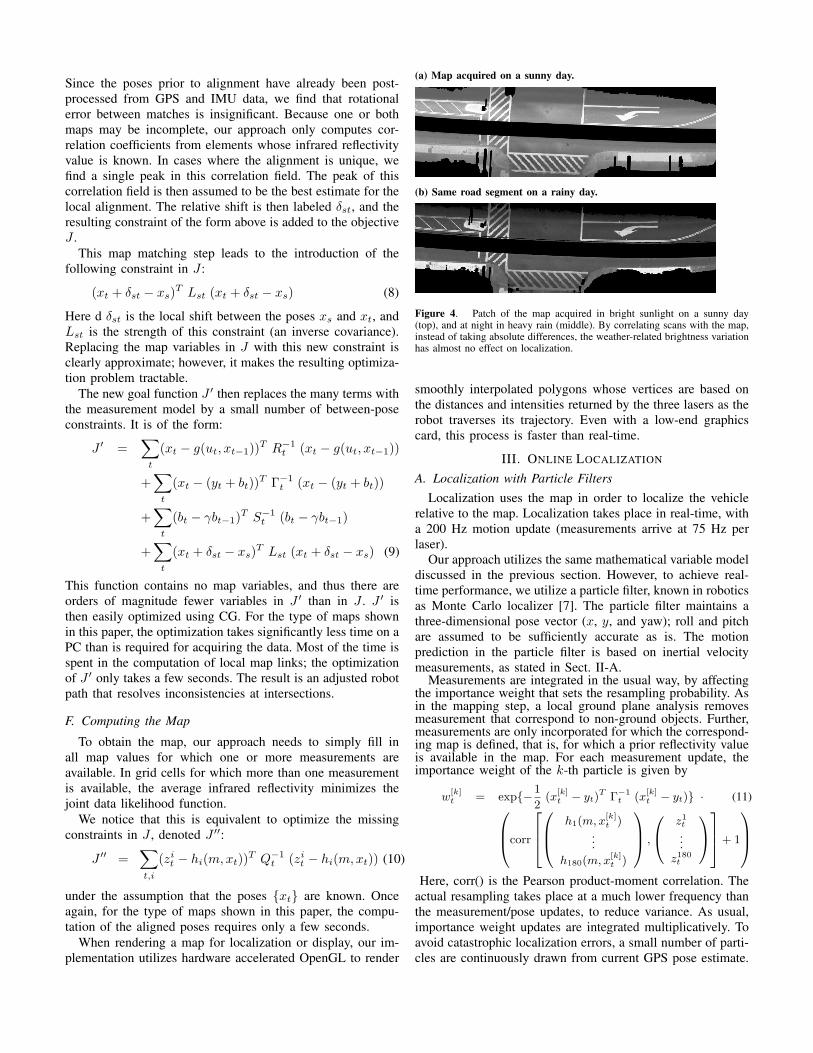
(a) Map acquired on a sunny day.

(b) Same road segment on a rainy day.

Figure 4. Patch of the map acquired in bright sunlight on a sunny day(top), and at night in heavy rain (middle). By correlating scans with the map,instead of taking absolute differences, the weather-related brightness variationhas almost no effect on localization.

smoothly interpolated polygons whose vertices are based on

the distances and intensities returned by the three lasers as the

robot traverses its trajectory. Even with a low-end graphics

card, this process is faster than real-time.

III. ONLINE LOCALIZATION

A. Localization with Particle Filters

Localization uses the map in order to localize the vehicle

relative to the map. Localization takes place in real-time, with

a 200 Hz motion update (measurements arrive at 75 Hz per

laser).

Our approach utilizes the same mathematical variable model

discussed in the previous section. However, to achieve real-

time performance, we utilize a particle filter, known in robotics

as Monte Carlo localizer [7]. The particle filter maintains a

three-dimensional pose vector (x, y, and yaw); roll and pitch

are assumed to be sufficiently accurate as is. The motion

prediction in the particle filter is based on inertial velocity

measurements, as stated in Sect. II-A.Measurements are integrated in the usual way, by affecting

the importance weight that sets the resampling probability. Asin the mapping step, a local ground plane analysis removesmeasurement that correspond to non-ground objects. Further,measurements are only incorporated for which the correspond-ing map is defined, that is, for which a prior reflectivity valueis available in the map. For each measurement update, theimportance weight of the k-th particle is given by

w[k]t

= exp{−1

2(x

[k]t

− yt)T Γ−1

t (x[k]t

− yt)} · (11)

corr

h1(m, x[k]t

)...

h180(m, x[k]t

)

,

z1t

...

z180t

+ 1

Here, corr() is the Pearson product-moment correlation. The

actual resampling takes place at a much lower frequency than

the measurement/pose updates, to reduce variance. As usual,

importance weight updates are integrated multiplicatively. To

avoid catastrophic localization errors, a small number of parti-

cles are continuously drawn from current GPS pose estimate.

This “sensor resetting” trick was proposed in [23]. GPS, when

available, is also used in the calculation of the measurement

likelihood to reduce the danger of particles moving too far

away from the GPS location.

One complicating factor in vehicle localization is weather.

As illustrated in Fig. 4, the appearance of the road surface is

affected by rain, in that wet surfaces tend to reflect less infrared

laser light than do dry ones. To adjust for this effect, the

particle filter normalizes the brightness and standard deviation

for each individual range scan, and also for the corresponding

local map stripes. This normalization transforms the least

squares difference method into the computation of the Pearson

product-moment correlation with missing variables (empty

grid cells in the map). Empirically, we find that this local

normalization step is essential for robust performance .

We also note that the particle filter can be run entirely

without GPS, where the only reference to the environment

is the map. Some of our experiments are carried out in the

absence of GPS, to illustrate the robustness of our approach

in situations where conventional GPS-based localization is

plainly inapplicable.

B. Data Management

Maps of large environments at 5-cm resolution occupy a

significant amount of memory. We have implemented two

methods to reduce the size of the maps and to allow relevant

data to fit into main memory.

When acquiring data in a moving vehicle, the rectangular

area which circumscribes the resulting laser scans grows

quadratically with distance, despite that the data itself grows

only linearly. In order to avoid a quadratic space requirement,

we break the rectangular area into a square grid, and only save

squares for which there is data. When losslessly compressed,

the grid images require approximately 10MB per mile of road

at 5-cm resolution. This would allow a 200GB hard drive to

hold 20,000 miles of data.

Although the data for a large urban environment can fit on

hard drive, it may not all be able to fit into main memory.

Our particle filter maintains a cache of image squares near

the vehicle, and thus requires a constant amount of memory

regardless of the size of the overall map.

IV. EXPERIMENTAL RESULTS

We conducted extensive experiments with the vehicle shown

in Fig. 1. This vehicle is equipped with a state-of-the-art

inertial navigation system (GPS, inertial sensors, and wheel

odometry), and three down-facing laser range finders: one

facing the left side, one facing the right side, and one facing

the rear. In all experiments, we use a pixel resolution of 5cm.

A. Mapping

We tested the mapping algorithm successfully on a variety

of urban roads. One of our testing environments is an urban

area, shown in Fig. 5. This image shows an aerial view of

the testing environment, with the map overlayed in red. To

generate this map, our algorithm automatically identified and

aligned several hundreds match points in a total of 32 loops. It

corrected the trajectory and output consistent imagery at 5-cm

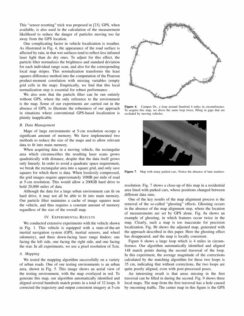
Figure 6. Campus Dr., a loop around Stanford 4 miles in circumference.To acquire this map, we drove the same loop twice, filling in gaps that areoccluded by moving vehicles.

Figure 7. Map with many parked cars. Notice the absence of lane markers.

resolution. Fig. 7 shows a close-up of this map in a residential

area lined with parked cars, whose positions changed between

different data runs.

One of the key results of the map alignment process is the

removal of the so-called “ghosting” effects. Ghosting occurs

in the absence of the map alignment step, where the location

of measurements are set by GPS alone. Fig. 8a shows an

example of ghosting, in which features occur twice in the

map. Clearly, such a map is too inaccurate for precision

localization. Fig. 8b shows the adjusted map, generated with

the approach described in this paper. Here the ghosting effect

has disappeared, and the map is locally consistent.

Figure 6 shows a large loop which is 4 miles in circum-

ference. Our algorithm automatically identified and aligned

148 match points during the second traversal of the loop.

In this experiment, the average magnitude of the corrections

calculated by the matching algorithm for these two loops is

35 cm, indicating that without corrections, the two loops are

quite poorly aligned, even with post-processed poses.

An interesting result is that areas missing in the first

traversal can be filled in during the second. Fig. 9 shows three

local maps. The map from the first traversal has a hole caused

by oncoming traffic. The center map in this figure is the GPS

Figure 5. (Best viewed in color) Aerial view of Burlingame, CA. Regions of overlap have been adjusted according to the methods described in this paper.Maps of this size tend not to fit into main memory, but are swapped in from disk automatically during driving.

(a) GPS leads to ghosting (b) Our method: No ghosting

Figure 8. Infrared reflectivity ground map before and after SLAM optimiza-tion. Residual GPS drift can be seen in the ghost images of the road markings(left). After optimization, all ghost images have been removed (right).

aligned map with the familiar ghosting effect. On the right is

the fused map with our alignment procedure, which possesses

no hole and exhibits no ghosting.

The examples shown here are representative of all the

maps we have acquired so far. We find that even in dense

urban traffic, the alignment process is robust to other cars

and non-stationary obstacles. No tests were conducted in open

featureless terrain (e.g., airfields without markings or texture),

as we believe those are of low relevance for the stated goal of

urban localization.

B. Localization

Our particle filter is adaptable to a variety of conditions.

In the ideal case, the vehicle contains an integrated GPS/IMU

system, which provides locally consistent velocity estimates

and global pose accuracy to within roughly a meter. In our

(a) Map with hole (b) Ghosting (c) Our approach

Figure 9. Filtering dynamic objects from the map leaves holes (left). Theseholes are often filled if a second pass is made over the road, but ghostimages remain (center). After SLAM, the hole is filled and the ghost imageis removed.

tests in a variety of urban roads, our GPS-equipped vehicle

was able to localize in real-time relative to our previously

created maps with errors of less than 10 cm, far exceeding the

accuracy with GPS alone.

We ran a series of experiments to test localization relative

to the learned map. All localization experiments used separate

data from the mapping data; hence the environment was sub-

ject to change that, at times, was substantial. In fact, the map

in Fig. 5 was acquired at night, but all localization experiments

took place during daylight. In our experimentation, we used

between 200 and 300 particles.

Fig. 10 shows an example path that corresponds to 20

minutes of driving and localization. During this run, the

average disagreement between real-time GPS pose and our

method was 66cm. Manual alignment of the map and the

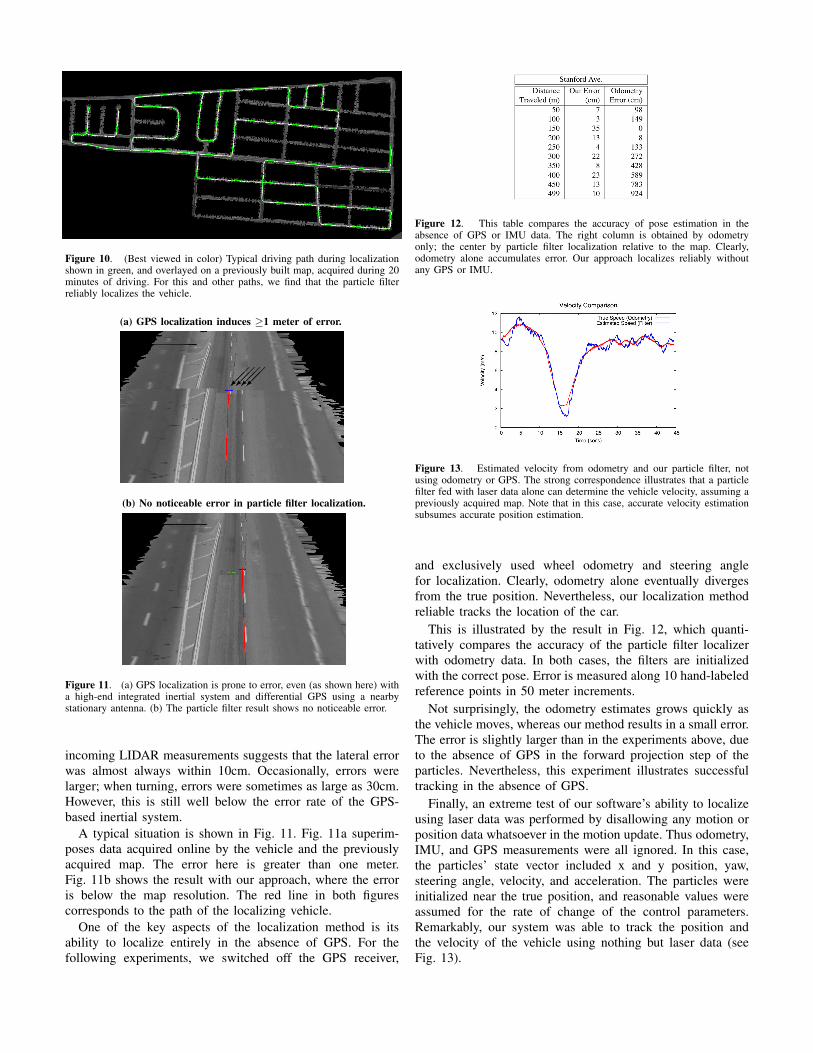
Figure 10. (Best viewed in color) Typical driving path during localizationshown in green, and overlayed on a previously built map, acquired during 20minutes of driving. For this and other paths, we find that the particle filterreliably localizes the vehicle.

(a) GPS localization induces ≥1 meter of error.

��������

(b) No noticeable error in particle filter localization.

Figure 11. (a) GPS localization is prone to error, even (as shown here) witha high-end integrated inertial system and differential GPS using a nearbystationary antenna. (b) The particle filter result shows no noticeable error.

incoming LIDAR measurements suggests that the lateral error

was almost always within 10cm. Occasionally, errors were

larger; when turning, errors were sometimes as large as 30cm.

However, this is still well below the error rate of the GPS-

based inertial system.

A typical situation is shown in Fig. 11. Fig. 11a superim-

poses data acquired online by the vehicle and the previously

acquired map. The error here is greater than one meter.

Fig. 11b shows the result with our approach, where the error

is below the map resolution. The red line in both figures

corresponds to the path of the localizing vehicle.

One of the key aspects of the localization method is its

ability to localize entirely in the absence of GPS. For the

following experiments, we switched off the GPS receiver,

Figure 12. This table compares the accuracy of pose estimation in theabsence of GPS or IMU data. The right column is obtained by odometryonly; the center by particle filter localization relative to the map. Clearly,odometry alone accumulates error. Our approach localizes reliably withoutany GPS or IMU.

Figure 13. Estimated velocity from odometry and our particle filter, notusing odometry or GPS. The strong correspondence illustrates that a particlefilter fed with laser data alone can determine the vehicle velocity, assuming apreviously acquired map. Note that in this case, accurate velocity estimationsubsumes accurate position estimation.

and exclusively used wheel odometry and steering angle

for localization. Clearly, odometry alone eventually diverges

from the true position. Nevertheless, our localization method

reliable tracks the location of the car.

This is illustrated by the result in Fig. 12, which quanti-

tatively compares the accuracy of the particle filter localizer

with odometry data. In both cases, the filters are initialized

with the correct pose. Error is measured along 10 hand-labeled

reference points in 50 meter increments.

Not surprisingly, the odometry estimates grows quickly as

the vehicle moves, whereas our method results in a small error.

The error is slightly larger than in the experiments above, due

to the absence of GPS in the forward projection step of the

particles. Nevertheless, this experiment illustrates successful

tracking in the absence of GPS.

Finally, an extreme test of our software’s ability to localize

using laser data was performed by disallowing any motion or

position data whatsoever in the motion update. Thus odometry,

IMU, and GPS measurements were all ignored. In this case,

the particles’ state vector included x and y position, yaw,

steering angle, velocity, and acceleration. The particles were

initialized near the true position, and reasonable values were

assumed for the rate of change of the control parameters.

Remarkably, our system was able to track the position and

the velocity of the vehicle using nothing but laser data (see

Fig. 13).

C. Autonomous Driving

In a series of experiments, we used our approach for semi-

autonomous urban driving. In most of these experiments, gas

and brakes were manually operated, but steering was con-

trolled by a computer. The vehicle followed a fixed reference

trajectory on a university campus. In some cases, the lane

width exceeded the vehicle width by less than 2 meters.Using the localization technique described here, the vehicle

was able to follow this trajectory on ten out of ten attempts

without error; never did our method fail to provide sufficient

localization accuracy. Similar experiments using only GPS

consistently failed within meters, illustrating that GPS alone is

insufficient for autonomous urban driving. We view the ability

to use our localization method to steer a vehicle in an urban

environment as a success of our approach.

V. CONCLUSIONS

Localization is a key enabling factor for urban robotic

operation. With accurate localization, autonomous cars can

perform accurate lane keeping and obey traffic laws (e.g., stop

at stop signs). Although nearly all outdoor localization work

is based on GPS, GPS alone is insufficient to provide the

accuracy necessary for urban autonomous operation.This paper presented a localization method that uses an

environment map. The map is acquired by an instrumented

vehicle that uses infrared LIDAR to measure the 3-D structure

and infrared reflectivity of the environment. A SLAM-style

relaxation algorithm transforms this data into a globally con-

sistent environment model with non-ground objects removed.

A particle filter localizer was discussed that enables a moving

vehicle to localize in real-time, at 200 Hz.Extensive experiments in urban environments suggest that

the localization method surpasses GPS in two critical di-

mensions: accuracy and availability. The proposed method

is significantly more accurate than GPS; its relative lateral

localization error to the previously recorded map is mostly

within 5cm, whereas GPS errors are often in the order of 1

meter. Second, our method succeeds in GPS-denied environ-

ments, where GPS-based systems fail. This is of importance

to navigation in urban canyons, tunnels, and other structures

that block or deflect GPS signals.The biggest disadvantage of our approach is its reliance

on maps. While road surfaces are relatively constant over

time, they still may change. In extreme cases, our localization

technique may fail. While we acknowledge this limitation, the

present work does not address it directly. Possible extensions

would involve filters that monitor the sensor likelihood, to

detect sequences of “surprising” measurements that may be

indicative of a changed road surface. Alternatively, it may be

possible to compare GPS and map-based localization estimates

to spot positioning errors. Finally, it may be desirable to

extend our approach to incorporate 3-D environment models

beyond the road surface for improved reliability and accuracy,

especially on unusually featureless roads.

REFERENCES

[1] C. Baker, A. Morris, D. Ferguson, S. Thayer, C. Whittaker, Z. Omohun-dro, C. Reverte, W. Whittaker, D. Hahnel, and S. Thrun. A campaignin autonomous mine mapping. In ICRA 2004.

[2] M. Bosse, P. Newman, J. Leonard, M. Soika, W. Feiten, and S. Teller.Simultaneous localization and map building in large-scale cyclic envi-ronments using the atlas framework. IJRR, 23(12), 2004.

[3] P. Cheeseman and P. Smith. On the representation and estimation ofspatial uncertainty. IJR, 5, 1986.

[4] DARPA. DARPA Grand Challenge rulebook, 2004. On the Web athttp://www.darpa.mil/grandchallenge05/Rules 8oct04.pdf.

[5] DARPA. DARPA Urban Challenge rulebook, 2006. On the Webat http://www.darpa.mil/grandchallenge/docs/Urban Challenge Rules121106.pdf.

[6] F. Dellaert, W. Burgard, D. Fox, and S. Thrun. Using the condensationalgorithm for robust, vision-based mobile robot localization. ICVP 1999.

[7] F. Dellaert, D. Fox, W. Burgard, and S. Thrun. Monte Carlo localizationfor mobile robots. ICRA 1999.

[8] E.D. Dickmanns. Vision for ground vehicles: history and prospects.IJVAS, 1(1) 2002.

[9] A Doucet. On sequential simulation-based methods for Bayesianfiltering. TR CUED/F-INFENG/TR 310, Cambridge University, 1998.

[10] T. Duckett, S. Marsland, and J. Shapiro. Learning globally consistentmaps by relaxation. ICRA 2000.

[11] H.F. Durrant-Whyte. Uncertain geometry in robotics. IEEE TRA, 4(1),1988.

[12] A. Eliazar and R. Parr. DP-SLAM: Fast, robust simultaneous localizationand mapping without predetermined landmarks. IJCAI 2003.

[13] J. Folkesson and H. I. Christensen. Robust SLAM. ISAV 2004.[14] U. Frese, P. Larsson, and T. Duckett. A multigrid algorithm for

simultaneous localization and mapping. IEEE Transactions on Robotics,2005.

[15] T.D. Gillespie. Fundamentals of Vehicle Dynamics. SAE Publications,1992.

[16] J. Guivant, E. Nebot, and S. Baiker. Autonomous navigation and mapbuilding using laser range sensors in outdoor applications. JRS, 17(10),2000.

[17] J.-S. Gutmann and K. Konolige. Incremental mapping of large cyclicenvironments. CIRA 2000.

[18] D. Hahnel, D. Fox, W. Burgard, and S. Thrun. A highly efficient Fast-SLAM algorithm for generating cyclic maps of large-scale environmentsfrom raw laser range measurements. IROS 2003.

[19] D. Hahnel, D. Schulz, and W. Burgard. Map building with mobile robotsin populated environments. IROS 2002.

[20] M. Hebert, C. Thorpe, and A. Stentz. Intelligent Unmanned GroundVehicles. Kluwer, 1997.

[21] K. Konolige. Large-scale map-making. AAAI, 2004.[22] B. Kuipers and Y.-T. Byun. A robot exploration and mapping strategy

based on a semantic hierarchy of spatial representations. JRAS, 8, 1991.[23] S. Lenser and M. Veloso. Sensor resetting localization for poorly

modelled mobile robots. ICRA 2000.[24] J. Leonard, J.D. Tardos, S. Thrun, and H. Choset, editors. ICRA

Workshop W4, 2002.[25] J. Liu and R. Chen. Sequential monte carlo methods for dynamic

systems. Journal of the American Statistical Association, 93. 1998.[26] M.A. Paskin. Thin junction tree filters for simultaneous localization and

mapping. IJCAI 2003.[27] M. Pitt and N. Shephard. Filtering via simulation: auxiliary particle

filter. Journal of the American Statistical Association, 94, 1999.[28] D. Pomerleau. Neural Network Perception for Mobile Robot Guidance.

Kluwer, 1993.[29] C. Thorpe and H. Durrant-Whyte. Field robots. ISRR 2001[30] S. Thrun and M. Montemerlo. The GraphSLAM algorithm with

applications to large-scale mapping of urban structures. IJRR, 25(5/6),2005.

[31] N. Tomatis, I. Nourbakhsh, and R. Siegwart. Hybrid simultaneouslocalization and map building: closing the loop with multi-hypothesistracking. ICRA 2002.

[32] I. Ulrich and I. Nourbakhsh. Appearance-based obstacle detection withmonocular color vision. AAAI 2000.

[33] C. Urmson, J. Anhalt, M. Clark, T. Galatali, J.P. Gonzalez, J. Gowdy,A. Gutierrez, S. Harbaugh, M. Johnson-Roberson, H. Kato, P.L. Koon,K. Peterson, B.K. Smith, S. Spiker, E. Tryzelaar, and W.L. Whittaker.High speed navigation of unrehearsed terrain: Red Team technology forthe Grand Challenge 2004. TR CMU-RI-TR-04-37, 2004.

[34] Bureau of Transportation Statistics U.S. Department of Transportation.Annual report, 2005.

[35] C.-C. Wang, C. Thorpe, and S. Thrun. Online simultaneous localizationand mapping with detection and tracking of moving objects: Theory andresults from a ground vehicle in crowded urban areas. ICRA 2003.