Embed Size (px)
Citation preview

Mapping aerial metal deposition in metropolitan areas from
tree bark: a case study in Sheffield, England
E. Schellea, B. G. Rawlins∗,b, R. M. Larkc, R. Websterc, I. Statona, C. W. Mcleod∗,a
aCentre for Analytical Sciences, Department of Chemistry, University of Sheffield,
Sheffield S3 7RF, UK
bBritish Geological Survey, Keyworth, Nottingham NG12 5GG, UK
cRothamsted Research, Harpenden, Hertfordshire AL5 2JQ, UK
∗ Corresponding authors:
B. G. Rawlins
British Geological Survey
Keyworth
Nottingham NG12 5GG
UK Telephone: +44 (0)
Fax: +44 (0)
e-mail: [email protected]
C. W. Mcleod
Centre for Analytical Sciences
Department of Chemistry
University of Sheffield
Dainton Building
Sheffield S3 7HF
UK
Telephone: +44 (0) 114 222 3602
Fax: +44 (0) 114 222 9379
1
ManuscriptClick here to download Manuscript: shefr.pdf

Abstract1
We investigated the use of metals accumulated on tree bark for mapping their2
deposition across metropolitan Sheffield by sampling 642 trees of three common species.3
Mean concentrations of metals were generally an order of magnitude greater than4
in samples from a remote uncontaminated site. We found trivially small differences5
among tree species with respect to metal concentrations on bark, and in subsequent6
statistical analyses did not discriminate between them. We mapped the concentrations7
of As, Cd and Ni by lognormal universal kriging using parameters estimated by residual8
maximum likelihood (reml). The concentrations of Ni and Cd were greatest close to9
a large steel works, their probable source, and declined markedly within 500 metres10
of it and from there more gradually over several kilometres. Arsenic was much more11
evenly distributed, probably as a result of locally mined coal burned in domestic fires12
for many years. Tree bark seems to integrate airborne pollution over time, and our13
findings show that sampling and analysing it are cost-effective means of mapping and14
identifying sources.15
Capsule: Multi-element analysis of tree bark can be effective for mapping the deposition16
of metals from air and relating it to sources of emission.17
Keywords: Multi-element analysis; Arsenic; Cadmium; Nickel; Geostatistics; REML;18
Universal kriging19
20
3
1. Introduction21
22
Inhalation of atmospheric aerosols, particularly of the fine size-fraction, can cause23
lung diseases, and regulatory standards exist to ensure that air quality meets interna-24
tionally defined standards. Airborne particulate matter (APM) for PM2.5 and PM10 is25
now widely monitored, particularly in urban environments. Nevertheless, government26
agencies and local authorities rarely have the resources to install equipment at the27
many sites that would be needed to map the spatial distribution of airborne particles.28
Normal practice for monitoring metals in APM is to establish installations at a few29
fixed locations, as in the Heavy Metals Monitoring Networks in the United Kingdom30
(Brown et al., 2007).31
Typical of this approach is the study of Moreno et al. (2004) who analysed APM32
at five sites in England and Wales. They showed that the air in Sheffield contained33
many metal-bearing particles in the <PM2.5 size-fraction. Those containing Cd and34
Ni are likely to derive from large steel works (Buse et al., 2003) and to impair health35
when inhaled. Attempts to apportion the particles to particular sources of metals in36
APM include chemical mass balance (Wang et al., 2006; Samara et al., 2003) and37
multivariate statistical analyses (Kim et al., 2006; Shah et al., 2006). Thomaidis et38
al. (2003) incorporated meteorological variables in their multivariate analysis because39
they found these influenced the concentrations of Cd, Ni and As in the APM in Athens.40
Sweet and Vermette (1993) studied anthropogenic emissions in urban Illinois based41
on trace metal data from three sites; they reported much temporal variation in the42
quantity of metal in the APM. They attributed this to variations in wind strength43
and direction, and the degree of atmospheric mixing. Atmospheric particulate matter44
in towns and cities is readily resuspended, and this process contributes significantly45
to temporal (Vermette et al., 1991) and spatial variation in the contents of metals46
(Kuang et al., 2004). So mapping the spatial distribution from direct measurements47
would require many permanent sampling installations to integrate concentrations over48
4

time.49
An attractive approach for mapping the long-term spatial distribution of elements50
in APM is by biomonitoring. The underlying idea is to let plants accumulate atmo-51
spheric depositions over time and then to analyse chemically the plant tissue. The52
scope for exploiting plants in this way is diverse and includes plant leaves, lichens,53
mosses and tree bark (Markert et al, 1993; Walkenhorst et al. 1993). The outer layer54
of tree bark, in particular, has been found to be an effective passive accumulator of55
airborne particles in both rural (Bohm et al., 1998) and urban (Tanaka and Ichikuni,56
1982) environments. The particles in question settle on the outer bark by wet and57
dry deposition, and they remain there until the tree sheds its bark, or are leached or58
washed away by rain, or a combination of the two.59
Smooth-barked trees in the northern temperate zone begin to shed their bark60
only when mature (after about 50 years); trees with rougher bark tend to shed theirs61
somewhat earlier. The metal species deposited in the outer bark are separated physi-62
cally from trace elements taken up in solution from the soil in the trees and their xylem63
by a layer of phloem and cambium (Martin and Coughtrey, 1982). Further, extraneous64
contamination from the soil itself is limited to lowest 1.5 m of the trunk. So pollutants65
in the bark above this height are almost entirely derived from the air (Wolterbeek and66
Bode, 1995).67
Determination of the metal contents of tree bark cannot lead to a direct as-68
sessment of air quality because such measurements are retrospective and integrate as69
averages over long times. Nevertheless, because trees are widespread in most towns70
and cities, sampling their bark for subsequent chemical analysis and then noting pre-71
cise locations mean that the elemental concentrations in the barks can be mapped.72
Such maps, whether simple displays of measured concentrations or ones made by more73
elaborate interpolation could point to the emitter(s) of the metals, and identify regions74
where much (and little) metal is deposited. To date there have been few published75
attempts to map the distributions of metals from the analysis of tree bark. One was by76
5
Lotschert and Kohm (1978) who drew isarithmic (‘contour’) maps of Pb and Cd based77
on samples from 34 ash trees (Fraxinus excelsior) throughout Frankfurt. A similar78
approach, adopted by Bellis et al. (2001) to map airborne emissions in the vicinity of79
a lead smelter, was based on plotting data on the enrichment in Pb. On a national80
scale Lippo et al. (1995) drew a ‘pollution’ map of Finland detailing anthropogenic81
emissions for cities and industrial regions.82
We have investigated the potential of tree bark for mapping the accumulated83
deposition of airborne metals across metropolitan Sheffield, a city which has more trees84
per unit of population than any other in Europe. We measured the concentrations of85
18 metal and metalloid elements in bark at 642 locations in the region and compared86
them with those at a virtually uncontaminated site (Mace Head, western Ireland) to87
determine the magnitude of contamination in the former. We collected bark samples88
from three tree species to determine whether there were any substantial differences in89
metal contents between them. We did a principal component analysis on the elements90
to establish the relationships between the elements and to discover whether there were91
particular groups of them that might behave differently from one another. We then92
chose three potentially toxic elements, namely Cd, As and Ni, as representatives and93
analysed their data spatially (a) to determine regional trends, (b) to estimate their94
spatial covariances, and (c) to interpolate and map their distributions by kriging. We95
have used these maps to identify likely local sources of atmospheric pollution. We96
discuss the wider implications of our findings for the use of tree bark in environmental97
monitoring.98
2. Materials and methods99
2.1 Study region, tree bark survey and analysis.100
Sheffield has a long tradition of iron smelting and the production of steel. The invention101
of the crucible process in 1740 sparked a massive expansion of the industry in the city,102
relying in part on coal from local mines, which continues to this day. This in turn led to103
6
severe air pollution before measures to combat it were introduced under the Clean Air104
Act of 1956. In 1963 the company British Steel opened a large works at Tinsley in the105
north east of the city (Figure 1) to make special steels. Its production, including that106
of stainless steel (ferrochrome), continues and emits significant quantities of Cr and Ni107
into the atmosphere. Gilbertson et al. (1997) reported on the long-term significance108
of metal emissions from steel manufacturing from their study of concentrations of Co,109
Cu, Fe, Ni, Pb, and Zn in a peat monolith from close to the works. They found110
extraordinarily large concentrations (in mg kg−1) of Cu (472), Ni (320), Pb (827) and111
Zn (613) compared to concentrations in soil from an urban survey of the city for which112
Rawlins et al. (2005) presented data for Pb and Ni. The study of Gilbertson et al.113
attributed the greatest enrichment of Cu and Zn in the uppermost layers to the works.114
The Environment Agency of the UK had compiled an inventory of pollution115
(Environment Agency, 2003) in which it registered the locations and quantities of116
atmospheric particulate metal emissions from static sources. The inventory included117
emissions exceeding the reporting thresholds of 100 g for Cd, 1 kg for As and 10 kg118
for Ni, each per year. It did not include sources of smaller amounts for which no119
information is available on metal composition. We collated the data for the Sheffield120
region and to 3 km beyond its boundary for the years for which data were available121
prior to our collection of the bark samples (1998–2002). We calculated the sum of122
emissions for the five years so that they could be presented as total emission figures123
(in kg) for each particular source.124
Below we discuss the significance of these sources in relation to the distributions125
of the metals in bark.126
In establishing the region for our current study we wished to encompass the127
major sources of metal emissions, including industry to the north and east of the City,128
whilst also estimating the spatial extent of metal deposition. We therefore surveyed129
an area extending across the city from the suburbs of Whirlow and Greenhill south130
and west of the centre and from which the prevailing wind blows (see wind rose inset131
7
in Figure 1) to industrial Brinsworth and Ecclesfield to the north-east of the city132
centre (see Figure 1). The number of people living in the region, estimated from133
the 1991 census, is approximately 271 500. This figure was calculated from the UK134
EDINA database of population-weighted centroids defined for all the 1991 enumeration135
districts (Bracken and Martin, 1989.). The total population of greater Sheffield is136
around 550 000.137
Samples of bark were collected from 642 trees of the three species (with pro-138
portions of each shown in parentheses): sycamore (Acer pseudoplatanus — 68%), oak139
(Quercus robur — 22%) and cherry (Prunus serrula — 10%); their locations are shown140
in Figure 1. Both sycamore and cherry have fairly smooth bark, whereas the bark of141
oak is rougher. The samples were collected between April and November, 2003. In142
a series of local neighbourhoods, trees belonging to the three species occurring in a143
public space were identified. From these a subset was sampled to provide, as far as144
possible, an even spatial distribution.145
Approximately 10 g of the external outer bark (1–2 mm depth) was removed from146
each target tree with a clean scraping tool at 1.5 m above the ground. Sample sites147
spanned an altitude range of 271 m, from 33 to 301 m above mean sea level. The mean148
altitude was 106 m.149
Trees in the temperate zone of the UK enlarge their diameters by approximately150
1 cm per year, so a tree’s circumference in cm divided by π gives an approximate age151
of the tree (P. Casey, personal communication). The ages of the trees from which bark152
was sampled ranged from 25 to 45 years (circumferences of 78 to 141 cm). Bark with153
moss, lichen or paint was excluded from the sample. The orientation of the location for154
sampling was random. The samplers wore polythene gloves to avoid contaminating the155
samples, which were stored in sealed brown paper envelopes at 4 ◦C. The geographic156
co-ordinates and altitude of each site were obtained by GPS (Garmin International,157
Inc., USA). A further nine bark samples were collected from sycamore trees at Mace158
Head on the west coast of Ireland (53◦ 20’ N, 9◦ 54’ W) so that we could estimate159
8
background concentrations where there is negligible pollution.160
Each bark sample was crushed into a fine powder in a Tema mill. The bark161
powder was then passed through a sieve (0.5 mm mesh) to remove any large lumps.162
Thereafter all the equipment was cleaned thoroughly to prevent cross-contamination of163
the following sample. Tree bark powder (4.0 g) was thoroughly mixed with polystyrene164
co-polymer binder (0.9 g) (Hoechst Wax, Spectro Analytical, UK) and pressed for 1165
minute to produce powder pellets. The powder pellets were analysed by EDXRF166
spectrometry (X-LAB, Spectro Analytical, UK). The instrument was calibrated for 18167
elements (Ag, Al, As, Ba, Cd, Co, Cr, Cu, Fe, Mn, Ni, Pb, Sb, Se, Sn, Ti, V, Zn) for168
a wide range of standard biological reference materials which included poplar leaves,169
lichen, human hair and tea leaves. Typical analytical performance has been published170
previously (Schelle et al., 2002). The concentrations of Cd were less than the detection171
limit for 19% of the samples, and so we set their values to half that limit for subsequent172
statistical analysis. Fifty two percent of the samples contained less than the detection173
limit of Ag, and so we do not consider it further.174
2.2 Summary statistics175
Table 1 summarizes the data for all 17 elements. The distribution of most was posi-176
tively skewed, some strongly, and so to stabilize variances for subsequent analyses we177
transformed the values to logarithms. The table lists the transformations we made.178
As expected, there is a huge range in the mean values. Aluminium, which is the179
most abundant metal in the rocks and soil, is most abundant in the bark also. Iron180
appears in large amounts, and given Sheffield’s history we might expect such results181
too. The concentrations of the other elements do not immediately stand out. With the182
exception of Al, the mean concentrations in Sheffield were much larger than those those183
at Mace Head (Table 2); for Cr, Mn, Ni and Ti they were an order of magnitude larger.184
Anthropogenic sources are almost certainly the reason for the greater concentrations185
of metal in the tree bark in Sheffield.186
What is highly significant is that the distributions of all the elements are strongly187
9

positively skewed, with skewness coefficients ranging from 1.7 to almost 10. We found188
that all could be described well by a three-parameter log-normal distribution, which189
has the probability density function:190
g(z) =1
σ(z − α)√
2πexp
[− 1
2σ2{ln(z − α)− µ}2
], (1)
where z is the variable of interest, µ and σ are the mean and standard deviation191
of the transformed variable, and α is the shift in the original scale to maximize the192
goodness of fit. The shift and the mean and standard deviations in natural logarithms193
are listed in Table 1. In the final column of Table 1 are the skewness coefficients194
of the logarithms from which it is evident that the transformations have made the195
distributions symmetric. This is important for stabilizing the variances, and we have196
done all our further analyses on these transformed scales.197
Analysis of variance revealed little differences among species; they accounted for198
less than 5% of the variance for any of 16 metals and for only 8.5% for As. We have199
therefore disregarded differences between species in our subsequent multivariate and200
spatial analysis.201
2.3 Selection of variables; principal component analysis.202
For the purpose of this paper we wanted to select a few elements from the 17 listed203
above that would illustrate both the feasibility of analysing APM in bark and mapping204
the distribution of elements in it and produce maps interesting in their own right.205
To help in the selection we did a principal component analysis on the correlation206
matrix of the logarithms. We hoped thereby to see any clusters of strongly correlated207
elements from which we could choose representatives and any other elements that were208
clearly uncorrelated with others and should be treated in their own right. Table 3 lists209
the leading eigenvalues of the correlation matrix. The first component accounts for210
almost half the variance, and second and third together account for more than half211
the remainder. Pursuing the analysis, we computed the correlation coefficients, rij,212
10

between the principal component scores and the (logarithms of the) original variables213
as214
rij = νij
√λj/σ2
i , (2)
where νij is the ith entry in the jth eigenvector, λj is the jth eigenvalue, and σ2i is the215
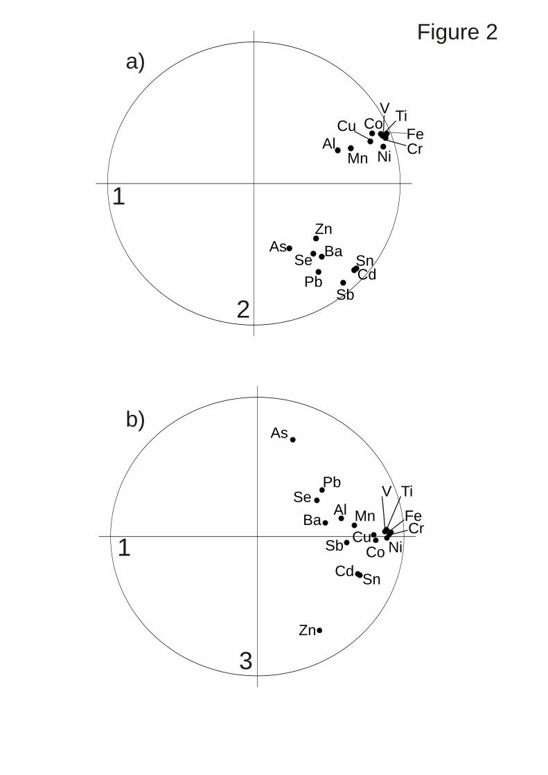
variance of the ith original variable. We then plotted the results in the unit circles for216
pairs of the leading components. We show two such circles in Figure 2 in which we217
have plotted the correlation coefficients (a) for component 2 against component 1 and218
(b) for component 3 against component 1. In general, the closer the points lie to the219
circumference of one of these circles the better are they represented in that projection.220
We note first that all of the plotted points fall in the right hand halves of the221
graphs: component 1 is essentially one of size. Component 2 discriminates, separating222
the siderophile (Fe, Mn, Co, Ni) and lithophile (Cr and V) elements from the calcophile223
group (Pb and Zn) and their associates. Arsenic appears nearest the centre in circle224
(a) and the least correlated with the other elements. This is confirmed in circle (b)225
in which the point for As lies close to the circumference and away from the other226
elements. Somewhat surprisingly Zn lies near the bottom of axis 3. The siderophiles227
remain clustered in this projection.228
From this examination of the data we have chosen three elements for our spatial229
analysis. We have chosen Ni as representative of the siderophiles and because it is a230
key element in steel production. We chose Cd because of its potential toxicity and231
again used in manufacturing. Third, we chose As, another poison, but from Figure232
2(b) clearly dissociated from the other elements.233
2.4 Spatial modelling by REML234
Our objective is to display the spatial variation of the three selected elements on235
tree bark across Sheffield as isarithmic (‘contour’) maps having first estimated the236
concentrations at the nodes of a fine grid. We used kriging for the estimation, following237
closely the technique we used to map the distribution of metals emitted from a smelter238
11

and described recently in this Journal (Rawlins et al., 2006).239
Ordinary kriging is based on two assumptions.240
1. A variable of interest, y, at locations xi, i = 1, 2, . . . , is a realization of an241
intrinsically stationary correlated random function Y (x) such that242
E [Y (x)− Y (x + h)] = 0 for all x, h , (3)
where E [·] denotes the statistical expectation of the term in brackets, and h is a243
lag vector, a displacement in space from the location x.244
2. The expected squared difference between Y (x) and Y (x + h) depends only on h:245
E[{Y (x)− Y (x + h)}2
]= 2γ(h) . (4)
The quantity γ(h) is the variance perpoint at lag h and as a function of h is the246
variogram.247
A preliminary display of the data for Ni and Cd at least suggested that the248
assumption in Equation (3) was not tenable; there were evident trends from small249
concentrations far from the steel works in the south west of the city to large ones close250
to the works in the north east, as we expected. This situation requires more complex251
geostatistical analysis in which the trend is separated from the random component252
and the estimates are made by universal kriging (Matheron, 1969), or ‘kriging with253
trend’ as it is now more generally known. Saito and Goovaerts (2001) encountered254
a similar problem in a study on the distribution of metal pollutants in two urban255
areas in the United States. In each case there were clear trends in the distribution256
of these contaminants, which could be accounted for by the wind direction and the257
location of sources (one smelter in one of the areas, and two adjacent smelters in the258
second). They used this information to produce simple trend models, based on physical259
principles, which predict the amount of metal that has been deposited from the sources260
at any location. This constituted the trend in their universal kriging. In order to model261
the spatial dependence of the random component, the residual from the trend, they262
12
estimated variograms of the pollutant from paired comparisons between sites at which263
the trend was deemed to be similar. This crudely filters the trend from the variogram264
that is obtained. It also discards the information about the random component of265
variation that could be obtained from comparisons between points where the trend is266
very different. To do this requires a more sophisticated analysis.267
Recent developments in numerical analysis linked to modern computing power268
enable us to use Residual Maximum Likelihood (reml) for the purpose, and we must269
now regard this as best practice. We described the procedure fully in Rawlins et al.270
(2006), and we shall not repeat the detail here. In this respect, then, our analysis271
was more sophisticated than that of Saito and Goovaerts (2001). In another respect272
it was more primitive, because we did not attempt to use a physically-based model273
for the trend in metal content of the bark. This was because, by contrast to the two274
regions studied by Saito and Goovaerts (2001), Sheffield has multiple sources of metal275
pollutants, and not only current or recent ones, but also many others from the distant276
past about which we have no detailed information. For our trend models therefore we277
considered only simple functions of the spatial coordinates.278
We treat the transformed data as the outcome from a mixed model:279
Y (x) =K∑
k=0
βkfk(x) + ε(x) . (5)
It consists of K + 1 fixed effects (which explain the trend in terms of known functions280
of the spatial co-ordinates) and a spatially dependent random variable ε(x) with mean281
zero and variogram γ(h). In order to apply reml to estimate the variance of the282
random variable and its spatial dependence we make stronger assumptions of station-283
arity than the intrinsic hypothesis stated in Equations (3) and (4) above. We require284
that the random variable is second-order stationary, which means that the variogram285
is bounded by the a priori variance of the process. This is not a serious constraint in286
practice once we have separated out the fixed effects, and is met by most of the popular287
variogram models used in geostatistics. Our task is to estimate the contributions of288
the fixed and random components simultaneously, minimizing the estimation variance.289
13

The separate contributions need not be explicitly computed when we use universal290
kriging, but they should be inspected to assess the weight of evidence for a trend in291
the variable.292
We first chose a few plausible models for the trend in Equation (5) by inspection293
of the data. We then separated these trends from the data and computed experimental294
variograms of the residuals by the usual method of moments:295
γ(h) =1
2m(h)
m(h)∑j=1
{y(xj)− y(xj + h)}2 , (6)
where y(xj) and y(xj +h) are the values of y at sampling points xj and xj +h separated296
by the lag h andm(h) is the number of paired comparisons at that lag. We fitted several297
of the standard simple models to these variograms by weighted least squares and chose298
the ones that fitted best in the least squares sense.299
This estimation of the trend ignores the spatial correlation of the residuals, but300
is acceptable for exploratory purposes. We found that we could describe the trend in301
the transformed data simply by the distance from a reference site in the north-east of302
the region, so that our full model for the variation was303
Y (x) = β0 + β1||x− xR||+ ε(x) , (7)
where || · || denotes the Euclidean norm of the enclosed vector. The vector xR is304
the reference site close to the steel works in the north-east of the region with British305
National Grid co-ordinates (441945.8, 390339.4). We chose this model in preference to306
a more conventional linear function of the co-ordinates because it achieved at least as307
good an ordinary least-squares fit to the data with one fewer terms.308
We then computed the experimental variograms of the ordinary least-squares309
residuals and found that an isotropic exponential model with nugget gave a satisfactory310
fit. Its equation is311
γ(h) = c0 + c
{1− exp
(−ha
)}, (8)
in which c0 is the nugget variance, c is the sill of the correlated variance, a is a distance312
parameter and h = ||h|| is now a scalar in distance only. This model, which is widely313
14

used in geostatistics, increases asymptotically to its maximum, with an effective range314
of 3× a.315
We then used the ASreml program (Gilmour et al., 2002) to fit the model in316
Equation (7) to each variable. We specified an exponential correlation function, which317
corresponds to the exponential variogram in Equation (8). The program provides reml318
estimates of the parameters c0, c and a, and generalized least-squares estimates of the319
fixed effects. We tested the null hypothesis that the true value of the fixed effect for the320
trend, β1, is zero by computing the Wald statistic. This statistic is equivalent to the321
variance ratio for the predictor in an analysis of variance for an ordinary least-squares322
regression. However, we used the method of Kenward and Roger (1997) to compute an323
adjusted Wald statistic, and adjusted degrees of freedom in the denominator for the F324
test to allow for the spatial dependence of the residuals.325
2.5 Lognormal universal kriging326
For reasons described above we transformed the raw data, z(x), to approximately327
normally distributed variables, which we have denoted by y(x). These values were328
used to obtain predictions at points on a fine grid over the region by universal kriging.329
The universal kriging (UK) uses the specified fixed effects in the prediction and the330
covariance parameters estimated by reml. Note that for arsenic, for which the trend331
was effectively constant, the universal kriging predictions are the same as those from332
ordinary kriging since we estimate one fixed effect, β0, which is the mean.333
Universal kriging returns an estimate of the transformed random variable Y (x);334
but we require estimates on the scale of the original data z(x). As with any estimate335
derived from log-transformed data, we cannot simply back transform the estimates on336
the logarithmic scale; we must also correct for bias. Cressie (2006) has shown that the337
UK estimate of a log-normal variable Z ′(x0), based on the UK estimate Y (x0) of the338
corresponding Y , is339
Z ′(x0) = exp
{Y (x0) +
1
2σ2
UK − ψ0 −K∑
i=1
ψifi(x0)
}, (9)
15

where the ψ0, ψ1, . . . are Lagrange parameters from the UK system (see Rawlins et al.,340
2006). We therefore back-transformed our kriged estimates in this way.341
We kriged the log-transformed variables at the nodes of a 200-m square grid.342
For each variable we specified the fixed effects selected after the reml analysis, and343
the covariance parameters obtained from that analysis. All observations were used344
for kriging at all target sites because we wanted the trend model at all target sites345
to be the same as the overall trend model to which our variogram refers. Since the346
number of data is large, this could lead to difficulties with the inversion of a large347
matrix. Our program for obtaining the lognormal UK estimates uses a subroutine348
for matrix inversion (LINRG, from IMSL, Visual Numerics, 1997) that reports any349
conditioning problems. It did not do so. We then used Equation (9) to transform350
the estimates back to the original scale, and corrected for the shift constant, α, in351
the original log-transformation. A particular advantage of kriging, relative to other352
methods for spatial prediction such as arbitrarily weighted local averaging, is that353
the error variances of the predictions are minimized and also (generally) is known.354
Unfortunately, back-transformations of the variances in the logarithms to the original355
scale can be calculated only for the simple kriging case (Webster and Oliver, 2007).356
Nevertheless, because we know the prediction variances on the transformed scale we357
can compute confidence limits and transform them. This therefore is what we did; we358
computed the local 95% upper limits in the logarithms and transformed them to the359
original scale of measurement.360
3. Results and their interpretation361
3.1 Trend and variance models based on REML362
As above, we analysed the data for the three elements Ni, Cd and As. Their histograms363
appear in the top row of Figure 3 and are evidently strongly positively skewed. The364
middle row of histograms in the figure are of their logarithms; the transformation has365
conferred symmetry (see also Table 1) and left no outliers. Finally, in the bottom row366
16

of the figure are the histograms of the residuals of the transformed data of Ni and Cd367
from their trends. Again the residuals for Ni and Cd are symmetrically distributed with368
small coefficients of skewness (-0.17 and 0.03 respectively). This gives us confidence369
that the assumption of normality of the random process, implicit in our use of reml for370
estimation of the variance model, is plausible. They show that, under the logarithmic371
transform, our data contain no obvious marginal outliers that might distort the variance372
model or local estimates. Finally, they show that the residual variation has been373
diminished—the standard deviation of the residuals of Ni is 0.794 compared with 1.202374
in the logarithms and that of Cd is 0.796 compared with 1.091.375
The trend models fitted for each element, after log-transformation, are listed376
in Table 4. Note that for both nickel and cadmium the estimated coefficient β1 is377
negative, and that the null hypothesis that there is no trend can be rejected decisively378
because of the very small value of P in the Wald test. The negative coefficient implies379
that the larger concentrations of metals are near the reference site in the north-east380
of the region. All the registered sources of Ni and Cd emissions occur in the north-381
east of the region also. The source with the largest emission of Ni (having emitted382
a total of 10 800 kg from 1998 to 2002) by almost one order of magnitude is 2.6 km383
to the west of the reference site (Figure 4a). The same emitter was also the largest384
source of Cd (having emitted 227 kg over the same period; Figure 4b). When the385
wind blows from the north and east these metals are dispersed towards the south and386
west, accounting for the observed trend. We do not observe the same degree of trend387
in the pattern to the north and east because when the wind blows from the south388
and west — the dominant prevailaing direction — significant quantities of metals are389
deposited towards the northern and eastern boundaries of the study region, where the390
concentrations remain substantially greater than the near background values observed391
elsewhere.392
The analysis reveals that the random effect for both Cd and Ni has marked393
spatial dependence; more than half of their variances is spatially correlated to distances394
17

between 2 and 2.5 km. This suggests that there are factors causing this variation395
unexplained by the trend model and that it might be worth attempting to identify396
them. The largest concentrations of Ni and Cd occur close to their dominant sources,397
accounting for the spatial dependence at short distances (Figure 4a and b).398
In contrast, there was no evident spatial trend in the concentrations of arsenic,399
which is confirmed in the formal Wald test of the null hypothesis that β1 is zero. For400
this reason we computed a variance model for log-transformed arsenic with only one401
fixed effect, namely the mean. The variogram parameters for this model were used for402
the kriging prediction. Note that little more than a fifth of the variance is spatially403
correlated, and that to distances of approximately only 1.5 km.404
3.2 Maps of metal concentration in bark.405
Figure 4a shows much short-range variation of Ni in the north-east of the region, which406
we presume to result from emissions and deposition from both current steel works and407
ones now defunct over many years. This pattern and the mechanism accord with what408
we know of total soil Ni concentrations across the city from a recent geochemical survey409
(Rawlins et al., 2005). The Ni is most concentrated immediately to the west of the big410
steel works at Tinsley (440 km east, 390 km north; Figure 4a). Another smaller source411
(437 km east, 389 km north) might account for the large concentrations (400 mg kg−1)412
in its vicinity and to the north and east in the direction of the prevailing wind. There413
are two small areas with large Ni values (440 km east, 388 km north; 438 km east,414
387.5 km north) which, according to our database, do not have significant sources415
nearby. Nevertheless, there are within 500 m of these two locations industries that416
might emit Ni-bearing particles. Concentrations of Ni are generally small in the north417
and south-west the region where there are no recorded sources of pollution. This418
suggests that there is little long-range dispersal, resuspension and deposition of the419
metal.420
Let us now turn to Cd. Figure 4b shows the largest concentrations around two421
sources (437 km east, 388 km north), one where metal is produced and processed422
18

(having emitted a total of 69 kg from 1998 to 2002), the other an incinerator (having423
emitted 52 kg over the same period). Somewhat surprisingly, the concentrations are424
smaller near to the source of the largest emission (total emission 227 kg from 1998 to425
2002). As with Ni, the concentrations of Cd diminish rapidly within 500 m of these426
sources, with the larger values extending northeastwards. The spatial patterns of Cd427
concentrations alone do not appear to reflect the magnitude of local sources, but the428
temporally varying dispersal mechanisms which depend on the strength and direction429
of the wind and the height of the emissions. A single spatial outlier with a large430
concentration of Cd (21.1 mg kg−1) occurs to the south-west of the region (432 km431
east, 384 km north) in an entirely residential area, and we cannot explain it.432
The spatial distribution of arsenic (As) is considerably more complex than that433
of Ni and Cd. The largest As concentrations do not occur around the steelworks at434
Tinsley — the largest static emitter (Figure 4c) — but where there are no registered435
emissions of As (438 km east, 390 km north). This part of the region contains a mixture436
of residential housing, industry and recreation grounds. Fugitive emissions from the437
industrial sites could acccount for some of the arsenic. The concentrations diminish438
rapidly in their immediate vicinity, but more slowly at greater distances. A similar439
pattern is observed around another area of large concentrations (434 km east, 385 km440
north), where once again there are no registered sources of emissions and land use is441
dominantly residential. Arsenic is richer in coal from Sheffield (Yorkshire) than in coal442
from most other parts of Great Britain. From an analysis of 24 samples of coal from443
across the country, those from the two Yorkshire seams had As concentrations of 8.7444
and 37 mg kg−1, which equate to the 65th and 97th percentile of the As distribution445
(Spears and Zheng, 1999). Coal was mined and burnt in the City for at least 200 years446
before the last coal mine was closed and the Clean Air acts were implemented in the447
1960s. There would have been many local emitters of As, and the APM from those448
days might still be being resuspended and redistributed.449
4. Discussion450
19

The substantially larger mean concentrations of metals in tree bark across Sheffield451
than those at Mace Head indicate that most of the metal in Sheffield is of anthro-452
pogenic origin. We have also shown that differences between tree species, and any453
differences in the roughness of their bark, are unlikely to be significant in determining454
the concentrations of most metals. It should therefore be possible to use tree bark455
from other species in similar environmental biomonitoring studies without introducing456
significant error. This is likely to be advantageous where trees of any one species are457
sparse.458
The concentrations of Ni and Cd in the bark of trees in Sheffield show that aerial459
deposition of metal, and any subsequent resuspension, diminishes markedly within460
500 metres of the emitters, though there appears to be significant dispersal over sev-461
eral kilometres. This strengthens the case for biomonitoring of long-term atmospheric462
pollution via the analysis of tree bark in a cost-effective way and for identifying where463
the sources of pollution are.464
The marked autocorrelation observed in the spatial distributions of Cd and Ni465
(and also Cr, Co and Cu which we have not described here) indicates that measure-466
ments of metals in tree bark in industrial environments can be used to map long-term467
deposition of those metals from the atmosphere. By contrast, elements such as lead468
with widespread and even mobile sources, as from motor vehicles before lead was for-469
bidden in fuel in the year 2000, are not spatially correlated; their variograms are wholly470
nugget at the working scale and so interpolation by any means should not be attempted.471
The method we describe and have applied is entirely statistical, though underlain472
by general knowledge and understanding. We did not attempt to use a source-oriented473
chemical transport model. We recognize that incorporation of such a model could im-474
prove spatial predictions and aid our interpretation of the spatial patterns observed.475
That is the next logical step in our investigation of these data, and we plan to incorpo-476
rate such in formation into the linear mixed model that we have used here (see Stacey477
et al., 2007).478
20
Acknowledgements479
This paper is published with the permission of the Director of the British Geologi-480
cal Survey (Natural Environment Research Council). Elvio Schelle is grateful to the481
Universidade Federal de Mato Grosso (Chiaba, Brazil) for the funding to undertake482
his PhD study. R.M. Lark’s contribution was supported by the Biotechnology and483
Biological Sciences Research Council of the United Kingdom through its core strategic484
grant to Rothamsted Research. We thank Colin Powlesland and Alex Hole of the UK’s485
Environment Agency for providing data from the Pollution Inventory.486
References487
Bellis, D., Cox, A.J., Staton, I., McLeod, C.W., Satake, K., 2001. Mapping airborne488
lead contamination near a metals smelter in Derbyshire, UK: spatial variation of489
Pb concentration and ‘enrichment factor’ for tree bark. Journal of Environmental490
Monitoring 3, 512–514.491
Bohm, P., Wolterbeek, H., Verburg, T. Musilek, L., 1998. The use of tree bark492
for environmental pollution monitoring in the Czech Republic. Environmental493
Pollution 102, 243–250.494
Brown, R. J. C., Williams, M., Butterfield, D. M., Yardley, R. E., Muhunthan, D.,495
Goddard, S. 2007. Annual Report for 2006 on the UK Heavy Metals Monitoring496
Network. National Physical Laboratory Report DQL-AS 036.497
http://www.airquality.co.uk/archive/reports/cat13/0703280922 FINAL498
Defra UK Heavy Metals Network Annual Report 2006.pdf. Accessed 1st Octo-499
ber 2007.500
Bracken, I. Martin, D., 1989. The generation of spatial population distributions from501
census centroid data. Environment and Planning A 21, 537–543.502
Buse, A., Norris, D., Harmens, H., Bker, P., Ashenden, T., Mills, G., 2003. Heavy503
21
metals in European mosses: 2000/2001 survey.504
http://icpvegetation.ceh.ac.uk/metals report pdf.htm. Accessed 14th September505
2007.506
Cressie, N., 2006. Block kriging for lognormal spatial processes. Mathematical Geol-507
ogy 38, 413–443.508
Environment Agency, 2003. Environment Agency Pollution Inventory.509
http://maps.environment-agency.gov.uk/wiyby/dataSearchController510
topic=pollution&lang=. Accessed 4th December 2003.511
Gilbertson, D.D., Grattan, J.P., Cressey, M. Pyatt, F.B., 1997. An air-pollution512
history of metallurgical innovation in iron- and steel-making: A geochemical513
archive of Sheffield. Water, Air and Soil Pollution 100, 327–341.514
Gilmour, A.R., Gogel, B.J., Cullis, B.R., Welham, S.J., Thompson, R. 2002. ASReml515
User Guide, Release 1.0. VSN International, Hemel Hempstead516
Kenward, M.G., Roger, J.H. 1997. Small sample inference for fixed effects from517
restricted maximum likelihood. Biometrics 53, 983–997.518
Kim, M.K., Jo, W.K., 2006. Elemental composition and source characterization of air-519
borne PM10 at residences with relative proximities to metal–industrial complex.520
International Archives of Occupational and Environmental Health 80, 40–50.521
Kuang, C., Neumann, T., Norra, S., Stuben, D., 2004. Land use-related chemical522
composition of street sediments in Beijing. Environmental Science and Pollution523
Research 11, 73–83.524
Lippo, H., Poikolainen, J., Kubin, E. 1995. The use of moss, lichen and pine bark525
in the nationwide monitoring of atmospheric heavy metal deposition in Finland.526
Water, Air and Soil Pollution 85, 2241–2246.527
22

Lotschert, W., Kohm, H.J., 1978. Characteristics of tree bark as an indicator of528
high-immission areas: II. Contents of heavy metals. Oecologia 37, 121–132.529
Markert, B., 1993. Instrumental Analysis of Plants. In: B. Markert (Ed.), Plants as530
Biomoniots. VCH, Weinheim, pp. 65-103.531
Martin, M.H., Coughtrey, P.J., 1982. Biological monitoring of heavy metal pollutants.532
Applied Science Publishers, London.533
Matheron, G. 1969. Le krigeage universel. Cahiers du Centre de Morphologie534
Mathematique. Ecole des Mines de Paris, Fontainebleau.535
Moreno, T., Gibbons, W.,T. Jones, T., Richards, R., 2004. Geochemical and size vari-536
ations in inhalable UK airborne particles: the limitations of mass measurements.537
Journal of the Geological Society 161, 899–902.538
Rawlins, B. G., Lark, R. M., O’Donnell, K.E., Tye, A. M., Lister, T. R., 2005. The539
assessment of point and diffuse metal pollution from an urban geochemical survey540
of Sheffield, England. Soil Use and Management 21,353–362.541
Rawlins, B.G., Lark, R.M., Webster, R., O’Donnell, K.E., 2006. The use of soil542
survey data to determine the magnitude and extent of historic metal deposition543
related to atmospheric smelter emissions across Humberside, UK. Environmental544
Pollution 143, 416–426.545
Samara, C., Kouimtzis, T., Tsitouridou, R., Kanias, G., Simeonov, V., 2003. Chemi-546
cal mass balance source apportionment of PM10 in an industrialized urban area547
of Northern Greece. Atmospheric Environment 37, 41–54.548
Saito, H., Goovaerts, P., 2001. Accounting for source location and transport direction549
in geostatistical prediction of contaminants. Environmental Science and Tech-550
nology 35, 4823–4829.551
23

Schelle, E., Staton, I., Clarkson, P.J., Bellis, D.J. McLeod, C., 2002. Rapid multiele-552
ment analysis of tree bark by EDXRF. International Journal of Environmental553
Analytical Chemistry 82, 785–793.554
Shah, M.H., Shaheen, N.N., Jaffar, M., 2006. Characterization, source identification555
and apportionment of selected metals in TSP in an urban atmosphere. Environ-556
mental Monitoring and Assessment 114, 573–587.557
Stacey, K. F., Lark, R.M., Whitmore, A.P., Milne, A.E., 2007. Using a process model558
and regression kriging to improve predictions of nitrous oxide emissions from soil.559
Geoderma 135, 107–117.560
Spears, D.A., Zheng, Y., 1999. Geochemistry and origin of elements in some UK561
coals. International Journal of Coal Geology 38, 161–179.562
Sweet, C.W., Vermette, S.J., Landsberger, S., 1993. Soures of toxic trace elements in563
urban air in Illinois. Environmental Science and Technology 27, 2502–2510.564
Tanaka, J. Ichikuni, M., 1982. Monitoring of heavy metals in airborne particles by565
using bark samples of Japanese cedar collected from the metropolitan region of566
Japan. Atmospheric Environment 16, 2105–2108.567
Thomaidis, N.S., Bakeas, E.B., Siskos, P.A., 2003. Characterization of lead, cad-568
mium, arsenic and nickel in PM2.5 particles in the Athens atmosphere, Greece.569
Chemosphere 52, 959–966.570
Tye, A.M., Hodgkinson, E.S., Rawlins, B.G., 2006. Microscopic and chemical studies571
of metal particulates in tree bark and attic dust: evidence for historical atmo-572
spheric smelter emissions, Humberside, UK. Journal of Environmental Monitor-573
ing 8, 904–912.574
Vermette, S.J., Irvine, K.N., Drake, J.J., 1991. Temporal variability of the elemental575
composition in urban street dust. Environmental Monitoring and Assessment 18,576
69–77.577
24

Visual Numerics, 1997. IMSL Math Library. Visual Numerics, Houston, TX.578
Walkenhorst, A., Hagemeyer, J. Breckle, S.W., 1993. Passive monitoring of airborne579
pollutants, particularly trace metals, with tree bark. In: B. Markert (Ed.), Plants580
as Biomonitors. VCH, Weinheim, pp. 523-540.581
Wang, X.L., Sato, T., Xing, B.S., 2006. Size distribution and anthropogenic sources582
apportionment of airborne trace metals in Kanazawa, Japan. Chemosphere 65,583
2440–2448.584
Webster, R., Oliver, M.A., 2007. Geostatistics for Environmental Scientists, 2nd585
edition. John Wiley and Sons, Chichester.586
Wolterbeek, H.T. Bode, P., 1995. Strategies in sampling and sample handling in the587
context of large-scale plant biomonitoring surveys of trace element air pollution.588
Science of the Total Environment 176, 33–43.589
25

List of Figures and Captions
Figure 1. Location and species of trees in the region surveyed from which bark was
sampled (n = 642). Inset: windrose (source: British Meteological Office) showing
direction and strength for 84 662 observations at 146 m above mean sea level in
Sheffield.
Figure 2. Projections of the correlation between the 17 elements and principal com-
ponent scores into unit circles for (a) the first and second components, and (b)
the first and third components.
Figure 3. Histograms of raw data (top row), of data transformed to their natural
logarithms (centre row) and residuals from the trend for log-transformed data for
Ni and Cd (bottom row).
Figure 4. Isarithmic maps of (left) concentrations in bark (back-transformed estimate
of the conditional expectation) (right) backtransformed upper 95% confidence
limit for the conditional expectation. Also shown are the sources of cumulative
emissions from 1998 to 2002 in kg for each of the metals: (a) Ni – A(81), B(10800),
C(37), D(519), (b) Cd – A(1), B(227), C(0.4), D(0.5), E(69), F(52) and (c) As –
A(40), B(1), C(2.7), D(3.4).
26

Table 1 Means and standard deviations (Std dev.) in mg kg−1 of the amounts of
17 elements in the bark dust, and the means and standard deviations of their natural
logarithms after a shift of origin—see text.
Original measurements Log transforms
Element Mean Std dev. Skewness Shift Mean Std dev. Skewness
Al 9484 46461 7.77 45 7.902 1.103 1.18Ti 421 465 6.24 29.8 5.812 0.760 0.08V 24.9 17.2 3.60 5.3 5.701 0.861 −0.39
Cr 265 593 9.14 1.1 4.704 1.283 0.15Mn 280 360 9.01 11.25 5.349 0.767 0.14Fe 5712 5669 2.44 264.5 8.354 0.827 0.04Co 2.93 2.467 2.88 0.198 0.916 0.661 0.12Ni 65.0 141 12.0 0 3.412 1.202 0.06Cu 47.3 32.5 1.96 4.3 3.779 0.571 0.06Zn 152 185 8.38 3.4 4.771 0.781 0.24As 3.65 2.390 1.77 1.130 1.494 0.451 0.02Se 1.56 0.955 3.32 0.8 0.801 0.359 0.08Cd 1.401 3.621 9.97 0.02 −0.368 1.091 0.04Sn 3.19 3.973 3.18 0.12 0.732 0.942 0.14Sb 23.9 18.47 1.95 6.6 3.270 0.550 0.03Ba 245 241 4.39 12.6 5.273 0.721 0.14Pb 226 153 1.69 45 5.457 0.525 0.02
27
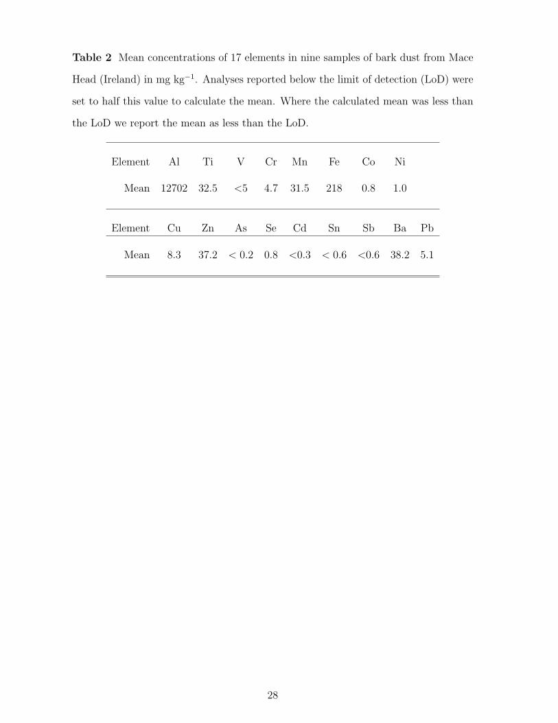
Table 2 Mean concentrations of 17 elements in nine samples of bark dust from Mace
Head (Ireland) in mg kg−1. Analyses reported below the limit of detection (LoD) were
set to half this value to calculate the mean. Where the calculated mean was less than
the LoD we report the mean as less than the LoD.
Element Al Ti V Cr Mn Fe Co Ni
Mean 12702 32.5 <5 4.7 31.5 218 0.8 1.0
Element Cu Zn As Se Cd Sn Sb Ba Pb
Mean 8.3 37.2 < 0.2 0.8 <0.3 < 0.6 <0.6 38.2 5.1
28
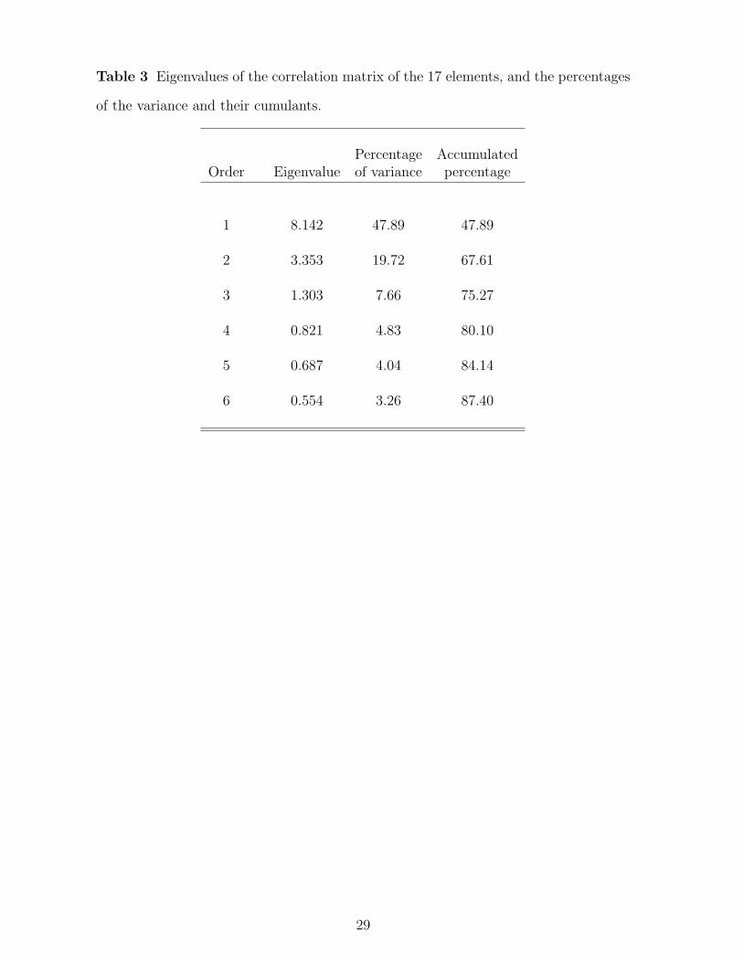
Table 3 Eigenvalues of the correlation matrix of the 17 elements, and the percentages
of the variance and their cumulants.
Percentage AccumulatedOrder Eigenvalue of variance percentage
1 8.142 47.89 47.89
2 3.353 19.72 67.61
3 1.303 7.66 75.27
4 0.821 4.83 80.10
5 0.687 4.04 84.14
6 0.554 3.26 87.40
29

Table 4 Results of the reml estimation of trend models for each element (log-
transformed), and reml variance model parameters for the model for arsenic with
no spatial trend.
Element Fixed effects Walda P valueb Estimated covariancestatistic parameters
β0 β1 a/metres c0 c
Ni 5.40 −0.277 106.1 0.55×10⁻⁶ 705 0.348 0.296
Cd 0.500 −0.135 18.9 2.22×10⁻³ 835 0.531 0.298
As 1.54 −0.003 0.11 0.75 558 0.156 0.047
As - - - 502 0.156 0.046
a Wald statistic for the fixed effect β1.
b Null hypothesis that β1 = 0.
30

Whirlow
Greenhill
Ecclesfield
Brinsworth
CherryOakSycamore
Tree bark sample locations
Survey area
Urban boundary
City centre
LowerDon valley
Wind strength(knots)
Wind direction
Figure 1
0 1 2 km
FigureClick here to download Figure: figs07.pdf
1
2
Al
TiV
CrMn
FeCo
Ni
Cu
ZnAs
SeCdSn
Sb
Ba
Pb
1
3
AlTiV
CrMn Fe
Co NiCu
Zn
As
Se
CdSn
Sb
Ba
Pb
Figure 2
a)
b)
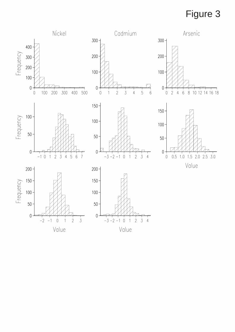
Figure 3

Figure 4a
430000 432000 434000 436000 438000 440000 442000
382000
384000
386000
388000
390000
392000
394000
A
B
C
D
0
250
500
750
1000
1250
mg kg-1
430000 432000 434000 436000 438000 440000 442000
382000
384000
386000
388000
390000
392000
394000
A
B
C
D
0
250
500
750
1000
1250
1500
1750
2000
2250
2500
mg kg-1
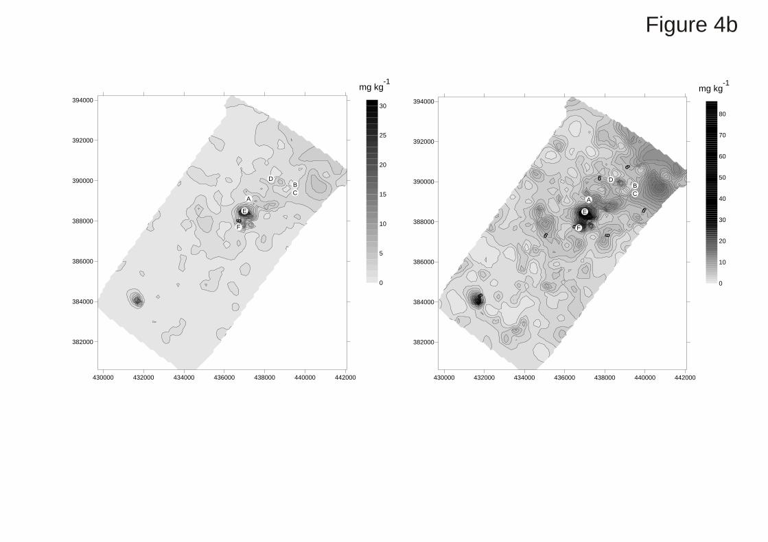
Figure 4b
430000 432000 434000 436000 438000 440000 442000
382000
384000
386000
388000
390000
392000
394000
A
B
C
D
E
F
0
5
10
15
20
25
30
mg kg-1
430000 432000 434000 436000 438000 440000 442000
382000
384000
386000
388000
390000
392000
394000
A
B
C
D
E
F
0
10
20
30
40
50
60
70
80
mg kg-1
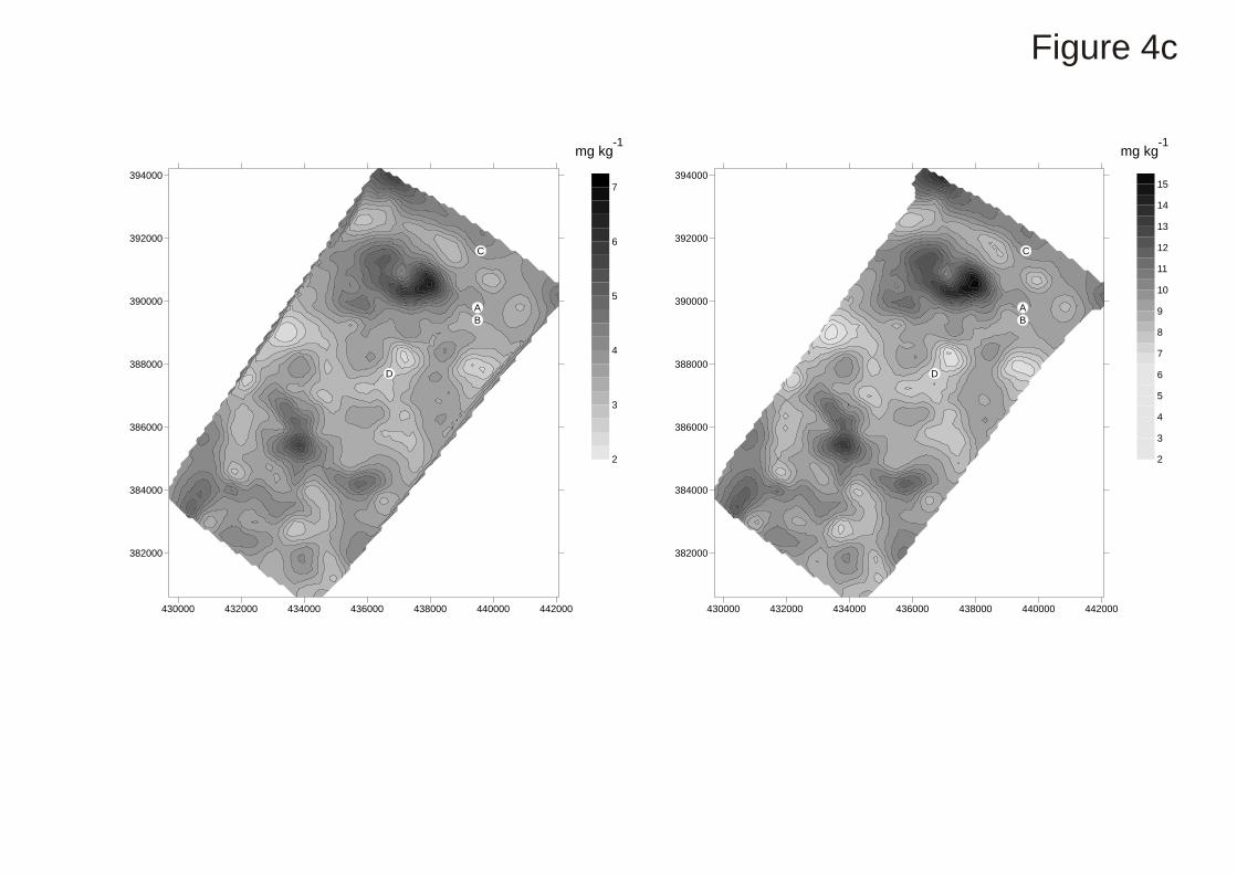
Figure 4c
430000 432000 434000 436000 438000 440000 442000
382000
384000
386000
388000
390000
392000
394000
A
B
C
D
2
3
4
5
6
7
mg kg-1
430000 432000 434000 436000 438000 440000 442000
382000
384000
386000
388000
390000
392000
394000
A
B
C
D
2
3
4
5
6
7
8
9
10
11
12
13
14
15
mg kg-1