MAPPING AND CHANGE ANALYSIS IN MANGROVE FOREST … · The mangrove map of USGS in 2011 Sundarbans, Bangladesh and India The Sundarbans delta is located on both sides of the border

MAPPING AND CHANGE ANALYSIS IN MANGROVE FOREST

BY USING LANDSAT IMAGERY

T. T. Dana*, C. F. Chenb, S. H. Chiangb, S. Ogawaa

a Graduate School of Engineering, Nagasaki University, Nagasaki, Japan –

[email protected], [email protected] b Centre for Space and Remote Sensing Research, National Central University, Taiwan –

[email protected], [email protected]

Commission VI, WG VI/4

KEY WORDS: Mangrove forest, Change detection, Image classification, Deforestation, Landsat data

ABSTRACT:

Mangrove is located in the tropical and subtropical regions and brings good services for native people. Mangrove in the world has been

lost with a rapid rate. Therefore, monitoring a spatiotemporal distribution of mangrove is thus critical for natural resource management.

This research objectives were: (i) to map the current extent of mangrove in the West and Central Africa and in the Sundarbans delta,

and (ii) to identify change of mangrove using Landsat data. The data were processed through four main steps: (1) data pre-processing

including atmospheric correction and image normalization, (2) image classification using supervised classification approach, (3)

accuracy assessment for the classification results, and (4) change detection analysis. Validation was made by comparing the

classification results with the ground reference data, which yielded satisfactory agreement with overall accuracy 84.1% and Kappa

coefficient of 0.74 in the West and Central Africa and 83.0% and 0.73 in the Sundarbans, respectively. The result shows that mangrove

areas have changed significantly. In the West and Central Africa, mangrove loss from 1988 to 2014 was approximately 16.9%, and

only 2.5% was recovered or newly planted at the same time, while the overall change of mangrove in the Sundarbans increased

approximately by 900 km2 of total mangrove area. Mangrove declined due to deforestation, natural catastrophes deforestation and

mangrove rehabilitation programs. The overall efforts in this study demonstrated the effectiveness of the proposed method used for

investigating spatiotemporal changes of mangrove and the results could provide planners with invaluable quantitative information for

sustainable management of mangrove ecosystems in these regions.

1. INTRODUCTION

Mangrove grows in river deltas, estuarine complexes and coasts

in the tropical and subtropical regions throughout the world. It

also inhabits on the shorelines and islands in sheltered coastal

areas with locally variable topography and hydrology (Lugo &

Snedaker, 1974). The total mangrove area accounts for 0.7% of

total tropical forests of the world. The largest extent of mangrove

is found in Asia (42.0%) followed by Africa (20.0%), North and

Central America (15.0%), Oceania (12.0%) and South America

(11.0%) (Giri et al., 2011). Mangrove is one of the most

threatened and vulnerability ecosystems. Based on the

importance and vulnerable of mangrove ecosystems faced, many

studies on mangrove have been conducted to solve these issues

in difference scales, long-term monitoring and detecting

mangrove by using remote sensing techniques (Blasco et al.,

2001; Everitt et al., 2008; Giri et al., 2007; Green, 1998; Seto &

Fragkias, 2007; and Vaiphasa et al., 2006).

The earth observation satellite data (such as Landsat) is useful for

change detection applications. The distribution and abundance of

mangrove in different regions of the world have been assessed

with a variety of techniques. The local variability of studies spans

all continents. Several studies have been carried out to investigate

and compare the suitability of various classification algorithms

for the spectral separation of mangrove. Change detection is a

powerful tool to visualize, measure, and better to understand a

trend in mangrove ecosystems. It enables the evaluation changes

over a long period of time as well as the identification of sudden

changes due to natural or dramatic anthropogenic impacts (for

example: tsunami destruction or conversion to shrimp farms).

Thus distribution, condition, and increase or decrease were the

measured features used in the change-detection applications of

mangrove. Monitoring change in mangrove was adopted by

many researchers throughout the world (Giri et al., 2011; Giri et

al., 2007; Ruiz-Luna and Berlanga-Robles, 2002; Concheddaa et

al., 2008; Selvam et al., 2003; Chen et al., 2013) and the

application of the supervised Maximum Likelihood Classifier

(MLC) was the most effective and robust method for classifying

mangroves based on traditional satellite remote sensing data.

African mangrove was widespread along the west coast from

Senegal to Congo that was interlinked with highly productive

coastal and tidal estuaries (UNEP, 2006). Regional conditions

enabled mangrove to grow as far as 100 kilometer inland, due to

strong tidal influences on rivers such as the River Gambia, the

Sine-Saloum delta in Senegal, and Guinea Bissau. The overall

trend for the region using area estimated from 1980 to 2006

indicated a moderate decline of mangrove covers. In the other

side, mangrove in the Southeast Asia (Sundarbans delta) is

located at the latitudes 21º30Ń to 22º30Ń, and longitudes

89º00É to 89º55É. They consist of about 200 islands, separated

by about 400 interconnected tidal rivers, creeks, and canals. The

Sundarbans declared as a Reserve Forest in 1875 and became the

UNESCO World Heritage Site in 1999. The mangrove of the

Sundarbans is dependent on natural regeneration for its existence.

The most important value of the Sundarbans lies in its protective

role. It helps hold coastlines, reclaim coastal lands, and settle the

silt carried by rivers. For this reason, the research was adopted to

detect spatial and temporal change in mangrove during the past

three decades, from 1988 to 2014 in two sites of study (West and

Central Africa and Sundarbans) by using a supervised

classification approach.

* Corresponding author

ISPRS Annals of the Photogrammetry, Remote Sensing and Spatial Information Sciences, Volume III-8, 2016 XXIII ISPRS Congress, 12–19 July 2016, Prague, Czech Republic

This contribution has been peer-reviewed. The double-blind peer-review was conducted on the basis of the full paper. doi:10.5194/isprsannals-III-8-109-2016

109

2. MATERIALS AND METHODS

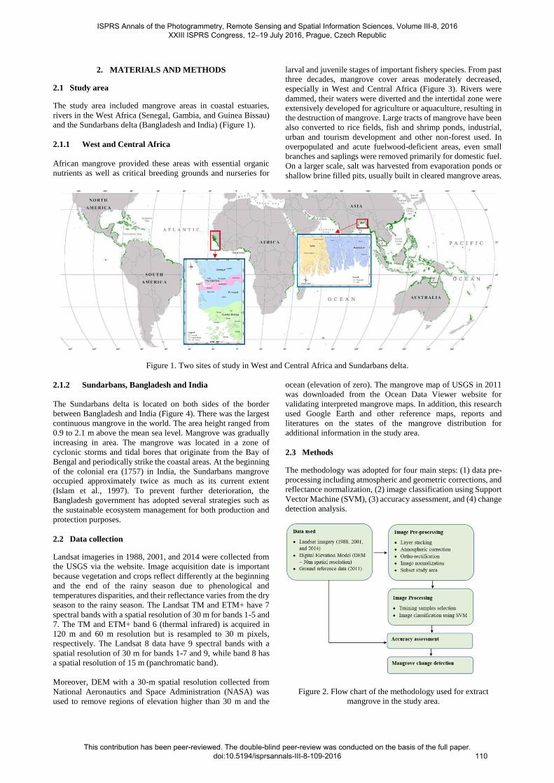
2.1 Study area

The study area included mangrove areas in coastal estuaries,

rivers in the West Africa (Senegal, Gambia, and Guinea Bissau)

and the Sundarbans delta (Bangladesh and India) (Figure 1).

2.1.1 West and Central Africa

African mangrove provided these areas with essential organic

nutrients as well as critical breeding grounds and nurseries for

larval and juvenile stages of important fishery species. From past

three decades, mangrove cover areas moderately decreased,

especially in West and Central Africa (Figure 3). Rivers were

dammed, their waters were diverted and the intertidal zone were

extensively developed for agriculture or aquaculture, resulting in

the destruction of mangrove. Large tracts of mangrove have been

also converted to rice fields, fish and shrimp ponds, industrial,

urban and tourism development and other non-forest used. In

overpopulated and acute fuelwood-deficient areas, even small

branches and saplings were removed primarily for domestic fuel.

On a larger scale, salt was harvested from evaporation ponds or

shallow brine filled pits, usually built in cleared mangrove areas.

Figure 1. Two sites of study in West and Central Africa and Sundarbans delta.

2.1.2 Sundarbans, Bangladesh and India

The Sundarbans delta is located on both sides of the border

between Bangladesh and India (Figure 4). There was the largest

continuous mangrove in the world. The area height ranged from

0.9 to 2.1 m above the mean sea level. Mangrove was gradually

increasing in area. The mangrove was located in a zone of

cyclonic storms and tidal bores that originate from the Bay of

Bengal and periodically strike the coastal areas. At the beginning

of the colonial era (1757) in India, the Sundarbans mangrove

occupied approximately twice as much as its current extent

(Islam et al., 1997). To prevent further deterioration, the

Bangladesh government has adopted several strategies such as

the sustainable ecosystem management for both production and

protection purposes.

2.2 Data collection

Landsat imageries in 1988, 2001, and 2014 were collected from

the USGS via the website. Image acquisition date is important

because vegetation and crops reflect differently at the beginning

and the end of the rainy season due to phenological and

temperatures disparities, and their reflectance varies from the dry

season to the rainy season. The Landsat TM and ETM+ have 7

spectral bands with a spatial resolution of 30 m for bands 1-5 and

7. The TM and ETM+ band 6 (thermal infrared) is acquired in

120 m and 60 m resolution but is resampled to 30 m pixels,

respectively. The Landsat 8 data have 9 spectral bands with a

spatial resolution of 30 m for bands 1-7 and 9, while band 8 has

a spatial resolution of 15 m (panchromatic band).

Moreover, DEM with a 30-m spatial resolution collected from

National Aeronautics and Space Administration (NASA) was

used to remove regions of elevation higher than 30 m and the

ocean (elevation of zero). The mangrove map of USGS in 2011

was downloaded from the Ocean Data Viewer website for

validating interpreted mangrove maps. In addition, this research

used Google Earth and other reference maps, reports and

literatures on the states of the mangrove distribution for

additional information in the study area.

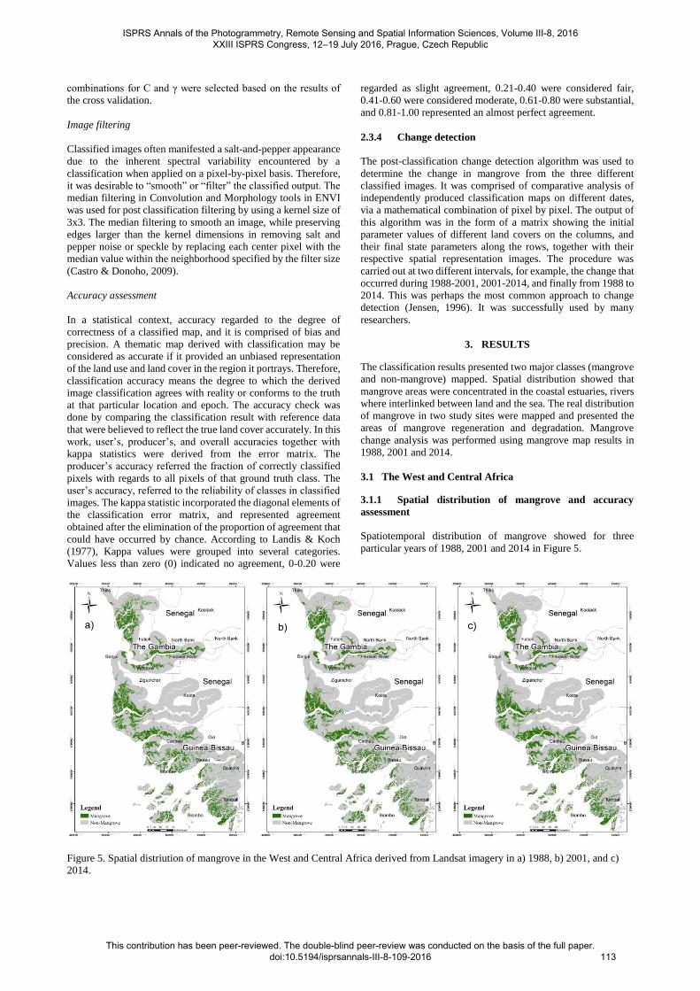
2.3 Methods

The methodology was adopted for four main steps: (1) data pre-

processing including atmospheric and geometric corrections, and

reflectance normalization, (2) image classification using Support

Vector Machine (SVM), (3) accuracy assessment, and (4) change

detection analysis.

Figure 2. Flow chart of the methodology used for extract

mangrove in the study area.



110

2.3.1 Image pre-processing

This research used all spectral bands and NDVI (an additional

band) to perform image classification. Remotely sensed data

acquired showed some forms of distortion or shift in geometric

location from one sensor to the other. Thus, image registration

was necessary to fix this problem. Image registration can be

defined as the transformation of an image or a map with respect

to another so that the properties of any resolution elements of the

object image addressable by the same coordinate pair in either

one of the images (Cideciyan et al., 1992). Ground control points

were used to correct geometric and a root mean square error

(RMSE) of 0.58 and 0.81 pixels were obtained in the West and

Central Africa and in the Sundarbans delta, respectively.

Landsat TM and ETM+ used Climate Data Records (CDR)

products. The surface reflectance CDR generated from

specialized software called Landsat Ecosystem Disturbance

Adaptive Processing System (LEDAPS). The software applies

MODIS atmospheric correction routines to Level-1 Landsat TM

or ETM+ data. Water vapor, ozone, geopotential heights, aerosol

optical thickness, and digital elevations were input with Landsat

data to the Second Simulation of a Satellite Signal in the Solar

Spectrum (6S) radiative transfer models to generate the top of

atmosphere (TOA) reflectance, surface reflectance, brightness

temperature, and to mask clouds, cloud shadows, adjacent

clouds, land, and water. Therefore, the atmospheric correction

only performed for Landsat 8 using Actor 2 (flat terrain, two

geometric degrees-of-freedom (DOF)) software. The detailed

parameters applied for the atmospheric correction presented in

Table 1.

Table 1. Parameters used for atmospheric correction model.

As the results of image acquisition, the date determined image

quality. They had different imageries on different dates in one

period. Thus, reflectance normalization was performed with a

histogram matching model which was developed by using

ERDAS IMAGINE. The result of reflectance normalization is

shown in Figure 3. Furthermore, two sites of the study were a

very big size. It covered by two images in the Sundarbans and

four images in the West and Central Africa. Hence, the subset

study area was reduced the bulk and the size of information was

processed. This reduced the time consumed for the analysis of

satellite images and also speeded up processing due to small

amount of processed data.

2.3.2 Masking out non-vegetation and height

Because of consideration on mangrove areas, non-vegetated

areas (such as water bodies, urban, and bare land) and heights

should be masked out. Non-vegetated areas were masked out by

using Normalized Difference Vegetation Index (NDVI). The

areas with its value less than 0.2 were masked out. This selected

a threshold to check by comparing the masking results with the

ancillary map, and reliable excluded for separating vegetated and

non-vegetated areas in Landsat images. Furthermore, mangrove

in two areas were mainly distributed in the coastal estuaries.

Based on the characteristics, the distribution of mangrove and the

ground reference map in 2011, mangrove was normally located

in areas where the elevation was lower than 30 m (Chen et al.,

2013). Therefore, the research was eliminated the areas higher

than 30 m in both two sites of the study (Figure 4). In the other

hand, buffer zone from the coastlines were generated. The buffer

distance was different in each continental, depending the spatial

distribution of mangrove on that region. In this case, 18-km, and

5-km buffers were used for West and Central Africa and the

Sundarbans delta.

2.3.3 Image classification

Training samples selection

From the training samples, they identified examples of land cover

types of interest on the image. The image processing software

system was then used to develop a statistical characterization of

the reflectance each class. The image was classified by

examining the reflectance each pixel and made a decision for

which of the signatures it resembled the most (Eastman, 1995).

For each study period, the Region of Interest (ROI) tool that

provided in ENVI was used to select the training samples.

Totally, there were six selected ROIs, including mangrove,

cultivation, vegetation, forest, bare land and water. Each ROI

represented a land cover category.



111

Figure 4. Study area after performing pre-processing and masking out non-vegetation area. a) Study area, b) Landsat image in 1988,

c) Landsat image in 2001, and d) Landsat image in 2014 (band combination: R=NIR, G=R, R=B).

Evaluation training samples

A separability test is one of methods to determine how similar

the distributions for two groups of pixels are. The Jefferies-

Matusita (JM) distance was a function of separability that directly

related to the probability of how good a resultant classification

will be (Swain et al., 1971). As the results of training data

selection, they were evaluated for agreement to classify the

images by using the JM from the following form:

In which is the Bhattacharya Distance and is given by

where i and j are the two signature classes,

is the mean vector signature for class ,

is corresponding class covariance matrix signature,

is the transposition function.

The JM distance had values 0 to 2. If JM value was greater than

1.9, then the classes show good separability. If values are

between 1.7 - 1.9, the separation between the classes was fairly

good below 1.7, the classes were poorly separated (Jensen, 1996).

Image classification

The Support Vector Machine (SVM) algorithm was a non-

parametric classifier. The method based on statistical learning

theory using a kernel function to non-linearly project the training

data in the input space into a higher dimensional space, where the

classes were linearly separable. The SVM has been widely

applied in remote sensing for classification of land uses or land

cover types. It has been demonstrated to give better classification

results among the maximum likelihood, univariate decision trees,

and back-propagation neural networks (Huang et al., 2002).

Nevertheless, it was also claimed that using the SVM for

classifying high-dimensional datasets can produce more accurate

results comparing with the traditional classifiers, but the outcome

greatly depends on the kernel types used, the choice of

parameters for the chosen kernel and the method used to generate

the SVM.

Chen and Ho (2008) provided an excellent general reference for

statistical learning in remote sensing. For linearly not separable

cases, the input data were mapped into a high dimensional space,

using so-called a kernel function. A training data set of samples,

in a d-dimensional feature space d, was given by xi with their

corresponding class labels:

The linear hyperplane f(x) was given by the normal vector w and

the bias b, with as a distance between the hyperplane and

the origin, where was the Euclidean norm of w, given by

next.

fl(x) = wx + b

The margin maximization leaded to the following optimization

problem:

where ζi: denoted the slack variables, and

C: the regularization parameter, which is used to penalize

training errors.

The SVM decision function for a non-linear separable case was

described by

where αi was Lagrange multipliers.

The kernel function k(xi,xj) performed a mapping operation and

enabled us to work within the newly transformed feature space,

only knowing the kernel function. A common kernel function in

remote sensing applications was the Gaussian radial basis

function (RBF), defined by

The training of an SVM classifier required the adequate

definition of the kernel parameter γ and the regularization

parameter C. The constant C was used as a penalty for training

samples that are located on the wrong side of the hyperplane. It

controlled the shape of the solution. Thus, it affected the

generalization capability of the SVM. However, the use of

inadequate parameter values might result in a less accurate

classification. Often the kernel parameters were determined by a

grid-search, using n-fold cross validation. Potential combinations

of C and γ were tested in a user-defined range and the best

(1)

(2) (5)

(3)

(4)

(6)

(7)



112

http://www.sciencedirect.com/science/article/pii/S0924271610001140#br000135

combinations for C and γ were selected based on the results of

the cross validation.

Image filtering

Classified images often manifested a salt-and-pepper appearance

due to the inherent spectral variability encountered by a

classification when applied on a pixel-by-pixel basis. Therefore,

it was desirable to “smooth” or “filter” the classified output. The

median filtering in Convolution and Morphology tools in ENVI

was used for post classification filtering by using a kernel size of

3x3. The median filtering to smooth an image, while preserving

edges larger than the kernel dimensions in removing salt and

pepper noise or speckle by replacing each center pixel with the

median value within the neighborhood specified by the filter size

(Castro & Donoho, 2009).

Accuracy assessment

In a statistical context, accuracy regarded to the degree of

correctness of a classified map, and it is comprised of bias and

precision. A thematic map derived with classification may be

considered as accurate if it provided an unbiased representation

of the land use and land cover in the region it portrays. Therefore,

classification accuracy means the degree to which the derived

image classification agrees with reality or conforms to the truth

at that particular location and epoch. The accuracy check was

done by comparing the classification result with reference data

that were believed to reflect the true land cover accurately. In this

work, user’s, producer’s, and overall accuracies together with

kappa statistics were derived from the error matrix. The

producer’s accuracy referred the fraction of correctly classified

pixels with regards to all pixels of that ground truth class. The

user’s accuracy, referred to the reliability of classes in classified

images. The kappa statistic incorporated the diagonal elements of

the classification error matrix, and represented agreement

obtained after the elimination of the proportion of agreement that

could have occurred by chance. According to Landis & Koch

(1977), Kappa values were grouped into several categories.

Values less than zero (0) indicated no agreement, 0-0.20 were

regarded as slight agreement, 0.21-0.40 were considered fair,

0.41-0.60 were considered moderate, 0.61-0.80 were substantial,

and 0.81-1.00 represented an almost perfect agreement.

2.3.4 Change detection

The post-classification change detection algorithm was used to

determine the change in mangrove from the three different

classified images. It was comprised of comparative analysis of

independently produced classification maps on different dates,

via a mathematical combination of pixel by pixel. The output of

this algorithm was in the form of a matrix showing the initial

parameter values of different land covers on the columns, and

their final state parameters along the rows, together with their

respective spatial representation images. The procedure was

carried out at two different intervals, for example, the change that

occurred during 1988-2001, 2001-2014, and finally from 1988 to

2014. This was perhaps the most common approach to change

detection (Jensen, 1996). It was successfully used by many

researchers.

3. RESULTS

The classification results presented two major classes (mangrove

and non-mangrove) mapped. Spatial distribution showed that

mangrove areas were concentrated in the coastal estuaries, rivers

where interlinked between land and the sea. The real distribution

of mangrove in two study sites were mapped and presented the

areas of mangrove regeneration and degradation. Mangrove

change analysis was performed using mangrove map results in

1988, 2001 and 2014.

3.1 The West and Central Africa

3.1.1 Spatial distribution of mangrove and accuracy

assessment

Spatiotemporal distribution of mangrove showed for three

particular years of 1988, 2001 and 2014 in Figure 5.

Figure 5. Spatial distriution of mangrove in the West and Central Africa derived from Landsat imagery in a) 1988, b) 2001, and c)

2014.



113

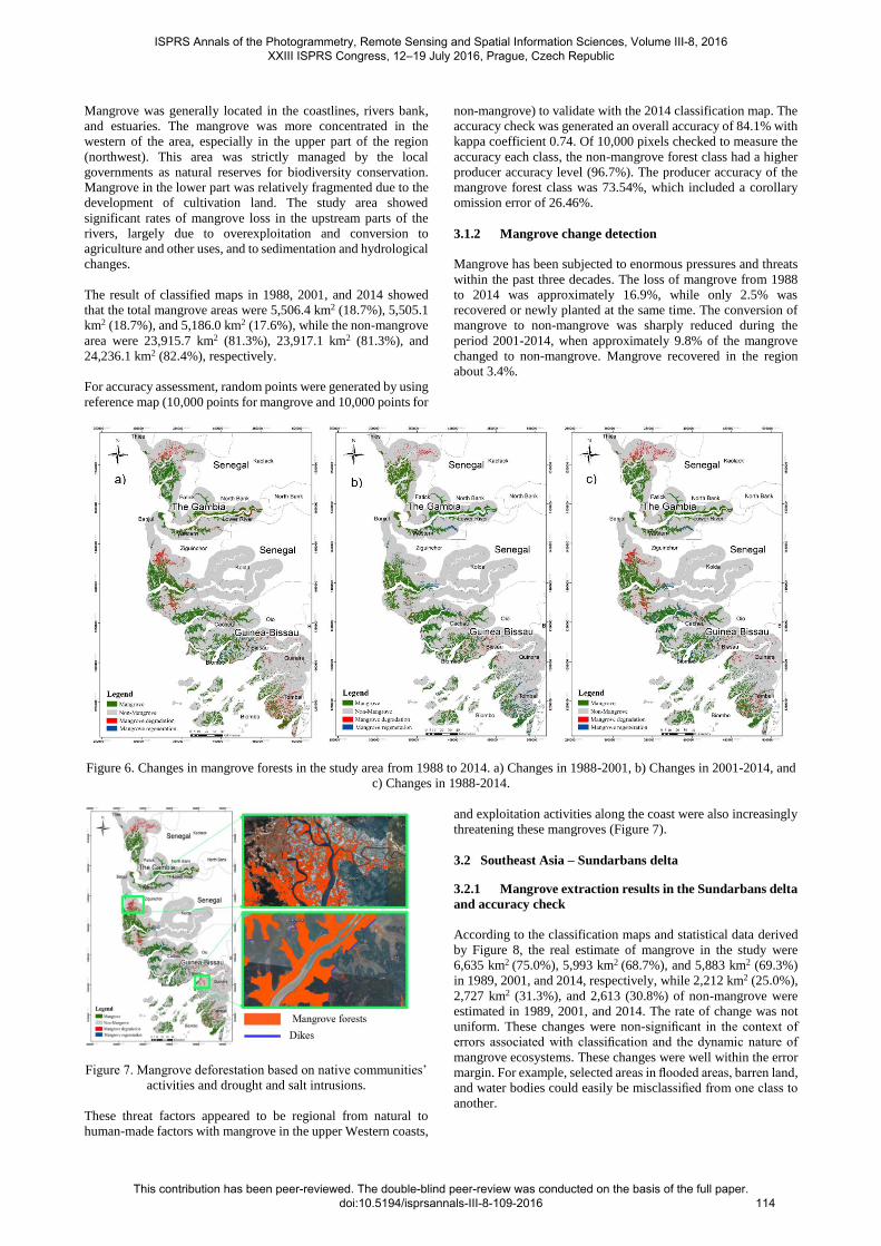
Mangrove was generally located in the coastlines, rivers bank,

and estuaries. The mangrove was more concentrated in the

western of the area, especially in the upper part of the region

(northwest). This area was strictly managed by the local

governments as natural reserves for biodiversity conservation.

Mangrove in the lower part was relatively fragmented due to the

development of cultivation land. The study area showed

significant rates of mangrove loss in the upstream parts of the

rivers, largely due to overexploitation and conversion to

agriculture and other uses, and to sedimentation and hydrological

changes.

The result of classified maps in 1988, 2001, and 2014 showed

that the total mangrove areas were 5,506.4 km2 (18.7%), 5,505.1

km2 (18.7%), and 5,186.0 km2 (17.6%), while the non-mangrove

area were 23,915.7 km2 (81.3%), 23,917.1 km2 (81.3%), and

24,236.1 km2 (82.4%), respectively.

For accuracy assessment, random points were generated by using

reference map (10,000 points for mangrove and 10,000 points for

non-mangrove) to validate with the 2014 classification map. The

accuracy check was generated an overall accuracy of 84.1% with

kappa coefficient 0.74. Of 10,000 pixels checked to measure the

accuracy each class, the non-mangrove forest class had a higher

producer accuracy level (96.7%). The producer accuracy of the

mangrove forest class was 73.54%, which included a corollary

omission error of 26.46%.

3.1.2 Mangrove change detection

Mangrove has been subjected to enormous pressures and threats

within the past three decades. The loss of mangrove from 1988

to 2014 was approximately 16.9%, while only 2.5% was

recovered or newly planted at the same time. The conversion of

mangrove to non-mangrove was sharply reduced during the

period 2001-2014, when approximately 9.8% of the mangrove

changed to non-mangrove. Mangrove recovered in the region

about 3.4%.

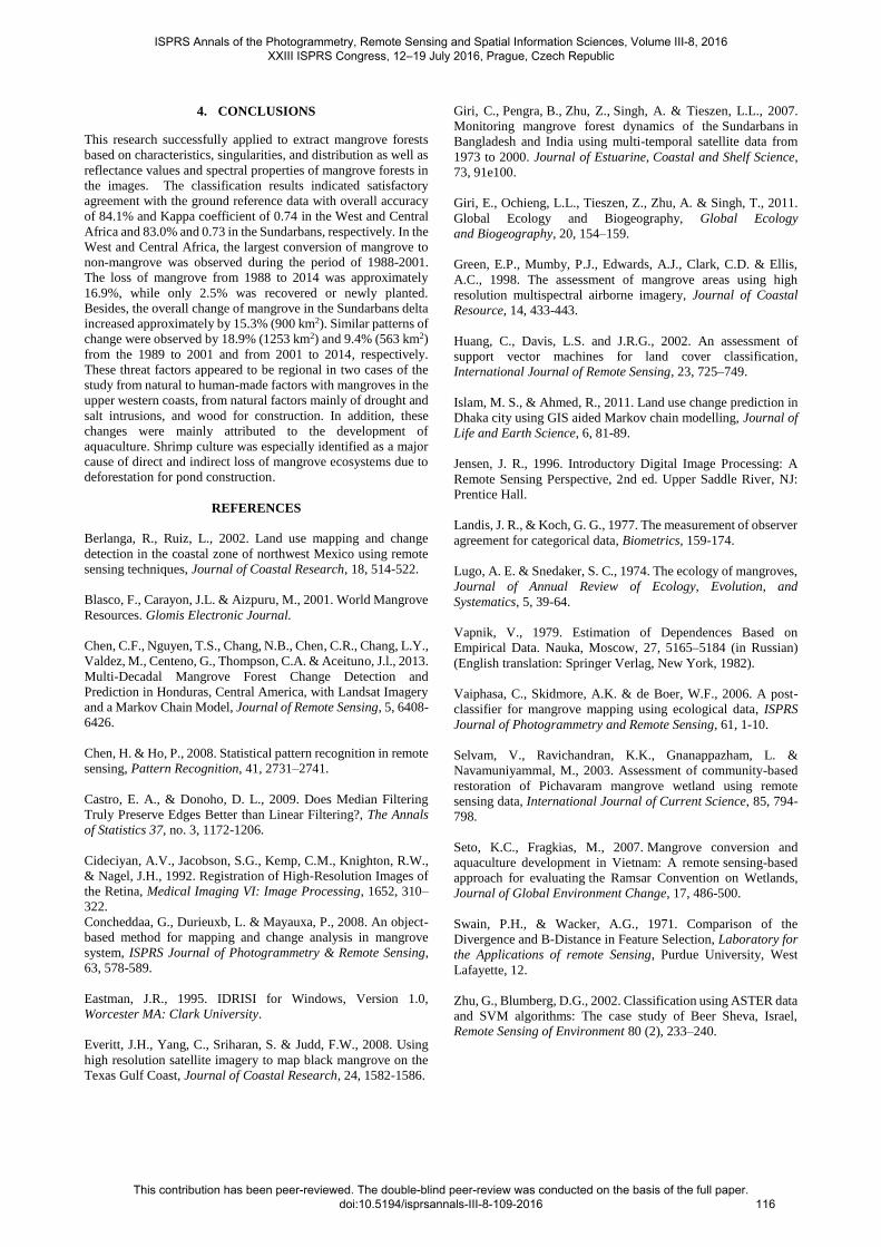
Figure 6. Changes in mangrove forests in the study area from 1988 to 2014. a) Changes in 1988-2001, b) Changes in 2001-2014, and

c) Changes in 1988-2014.

Figure 7. Mangrove deforestation based on native communities’

activities and drought and salt intrusions.

These threat factors appeared to be regional from natural to

human-made factors with mangrove in the upper Western coasts,

and exploitation activities along the coast were also increasingly

threatening these mangroves (Figure 7).

3.2 Southeast Asia – Sundarbans delta

3.2.1 Mangrove extraction results in the Sundarbans delta

and accuracy check

According to the classification maps and statistical data derived

by Figure 8, the real estimate of mangrove in the study were

6,635 km2 (75.0%), 5,993 km2 (68.7%), and 5,883 km2 (69.3%)

in 1989, 2001, and 2014, respectively, while 2,212 km2 (25.0%),

2,727 km2 (31.3%), and 2,613 (30.8%) of non-mangrove were

estimated in 1989, 2001, and 2014. The rate of change was not

uniform. These changes were non-significant in the context of

errors associated with classification and the dynamic nature of

mangrove ecosystems. These changes were well within the error

margin. For example, selected areas in flooded areas, barren land,

and water bodies could easily be misclassified from one class to

another.



114

Figure 8. Spatial distriution of mangrove forest in a) 1988, b) 2001, and c) 2014 in the Sundarbans delta derived from Landsat

imagery.

Table 2 presented the error matrix comparing the ground

reference map with 2014 classification map. The table showed

that the overall accuracy was 87.0% and the Kappa coefficient

was 0.73. The result explanted that mangrove class had a higher

producer accuracy level (91.0%). The producer accuracy of the

non-mangrove class was 76.0%, which included a corollary

omission error of 24.0%.

Reference data Classification result (2014)

Mangrove Non-Mangrove Total

Mangrove 881 100 981

Non-Mangrove 84 330 414

Total 965 430 1,395

Producer accuracy 91% 76%

User accuracy 89% 79%

Overall accuracy 87%

Kappa coefficient 0.73

Table 2. The error matrix for classification results in 2014

comparing with ground reference map in 2011 with some

modifications by the author.

3.2.2 Change in mangrove in the Sundarbans delta in

three past decades

The change of mangrove in three periods, 1989-2001, 2001-

2014, and 1989-2014 presented that the overall change of

mangrove in the Sundarbans delta dramatically increased by

approximately 15.3% (900 km2) of the total mangrove area from

non-mangrove areas and nature effected.

Similar patterns of change were observed 18.9% (1,253 km2) and

9.4% (563 km2) from the 1989 to 2001 and from 2001 to 2014

(Table 3), respectively. The classification results presented that

more than 90% of mangrove, and 75% of non-mangrove areas

did not change. But from 2001 to 2014, about 87% of mangrove

did not change. The large change between mangrove and non-

mangrove may possibly be due to variation in tidal inundation at

the time of satellite data acquisition. Non-mangrove areas were

found in the outer periphery in the Sundarbans. Due to

aggradation, land continues to be new in the Sundarbans. This

process had increased the land and mangrove areas. The most

dramatic and undeniable areas of change were found along

waterways in the Bay of Bengal, and some inland areas showed

evidence of change as well.

Table 3. Changes in the three past decades in Sundarbans.



115

4. CONCLUSIONS

This research successfully applied to extract mangrove forests

based on characteristics, singularities, and distribution as well as

reflectance values and spectral properties of mangrove forests in

the images. The classification results indicated satisfactory

agreement with the ground reference data with overall accuracy

of 84.1% and Kappa coefficient of 0.74 in the West and Central

Africa and 83.0% and 0.73 in the Sundarbans, respectively. In the

West and Central Africa, the largest conversion of mangrove to

non-mangrove was observed during the period of 1988-2001.

The loss of mangrove from 1988 to 2014 was approximately

16.9%, while only 2.5% was recovered or newly planted.

Besides, the overall change of mangrove in the Sundarbans delta

increased approximately by 15.3% (900 km2). Similar patterns of

change were observed by 18.9% (1253 km2) and 9.4% (563 km2)

from the 1989 to 2001 and from 2001 to 2014, respectively.

These threat factors appeared to be regional in two cases of the

study from natural to human-made factors with mangroves in the

upper western coasts, from natural factors mainly of drought and

salt intrusions, and wood for construction. In addition, these

changes were mainly attributed to the development of

aquaculture. Shrimp culture was especially identified as a major

cause of direct and indirect loss of mangrove ecosystems due to

deforestation for pond construction.

REFERENCES

Berlanga, R., Ruiz, L., 2002. Land use mapping and change

detection in the coastal zone of northwest Mexico using remote

sensing techniques, Journal of Coastal Research, 18, 514-522.

Blasco, F., Carayon, J.L. & Aizpuru, M., 2001. World Mangrove

Resources. Glomis Electronic Journal.

Chen, C.F., Nguyen, T.S., Chang, N.B., Chen, C.R., Chang, L.Y.,

Valdez, M., Centeno, G., Thompson, C.A. & Aceituno, J.l., 2013.

Multi-Decadal Mangrove Forest Change Detection and

Prediction in Honduras, Central America, with Landsat Imagery

and a Markov Chain Model, Journal of Remote Sensing, 5, 6408-

6426.

Chen, H. & Ho, P., 2008. Statistical pattern recognition in remote

sensing, Pattern Recognition, 41, 2731–2741.

Castro, E. A., & Donoho, D. L., 2009. Does Median Filtering

Truly Preserve Edges Better than Linear Filtering?, The Annals

of Statistics 37, no. 3, 1172-1206.

Cideciyan, A.V., Jacobson, S.G., Kemp, C.M., Knighton, R.W.,

& Nagel, J.H., 1992. Registration of High-Resolution Images of

the Retina, Medical Imaging VI: Image Processing, 1652, 310–

322.

Concheddaa, G., Durieuxb, L. & Mayauxa, P., 2008. An object-

based method for mapping and change analysis in mangrove

system, ISPRS Journal of Photogrammetry & Remote Sensing,

63, 578-589.

Eastman, J.R., 1995. IDRISI for Windows, Version 1.0,

Worcester MA: Clark University.

Everitt, J.H., Yang, C., Sriharan, S. & Judd, F.W., 2008. Using

high resolution satellite imagery to map black mangrove on the

Texas Gulf Coast, Journal of Coastal Research, 24, 1582-1586.

Giri, C., Pengra, B., Zhu, Z., Singh, A. & Tieszen, L.L., 2007.

Monitoring mangrove forest dynamics of the Sundarbans in

Bangladesh and India using multi-temporal satellite data from

1973 to 2000. Journal of Estuarine, Coastal and Shelf Science,

73, 91e100.

Giri, E., Ochieng, L.L., Tieszen, Z., Zhu, A. & Singh, T., 2011.

Global Ecology and Biogeography, Global Ecology

and Biogeography, 20, 154–159.

Green, E.P., Mumby, P.J., Edwards, A.J., Clark, C.D. & Ellis,

A.C., 1998. The assessment of mangrove areas using high

resolution multispectral airborne imagery, Journal of Coastal

Resource, 14, 433-443.

Huang, C., Davis, L.S. and J.R.G., 2002. An assessment of

support vector machines for land cover classification,

International Journal of Remote Sensing, 23, 725–749.

Islam, M. S., & Ahmed, R., 2011. Land use change prediction in

Dhaka city using GIS aided Markov chain modelling, Journal of

Life and Earth Science, 6, 81-89.

Jensen, J. R., 1996. Introductory Digital Image Processing: A

Remote Sensing Perspective, 2nd ed. Upper Saddle River, NJ:

Prentice Hall.

Landis, J. R., & Koch, G. G., 1977. The measurement of observer

agreement for categorical data, Biometrics, 159-174.

Lugo, A. E. & Snedaker, S. C., 1974. The ecology of mangroves,

Journal of Annual Review of Ecology, Evolution, and

Systematics, 5, 39-64.

Vapnik, V., 1979. Estimation of Dependences Based on

Empirical Data. Nauka, Moscow, 27, 5165–5184 (in Russian)

(English translation: Springer Verlag, New York, 1982).

Vaiphasa, C., Skidmore, A.K. & de Boer, W.F., 2006. A post-

classifier for mangrove mapping using ecological data, ISPRS

Journal of Photogrammetry and Remote Sensing, 61, 1-10.

Selvam, V., Ravichandran, K.K., Gnanappazham, L. &

Navamuniyammal, M., 2003. Assessment of community-based

restoration of Pichavaram mangrove wetland using remote

sensing data, International Journal of Current Science, 85, 794-

798.

Seto, K.C., Fragkias, M., 2007. Mangrove conversion and

aquaculture development in Vietnam: A remote sensing-based

approach for evaluating the Ramsar Convention on Wetlands,

Journal of Global Environment Change, 17, 486-500.

Swain, P.H., & Wacker, A.G., 1971. Comparison of the

Divergence and B-Distance in Feature Selection, Laboratory for

the Applications of remote Sensing, Purdue University, West

Lafayette, 12.

Zhu, G., Blumberg, D.G., 2002. Classification using ASTER data

and SVM algorithms: The case study of Beer Sheva, Israel,

Remote Sensing of Environment 80 (2), 233–240.



116

Documents

MAPPING AND CHANGE ANALYSIS IN MANGROVE FOREST … · The mangrove map of USGS in 2011 Sundarbans, Bangladesh and India The Sundarbans delta is located on both sides of the border