Mapping Free Energy in the Solar Atmosphere

14 Feb 2006 C4: Coronal Energy Inputs I.

Mapping Free Energy in the Solar AtmosphereWhat can we learn from HMI & AIA?

Brian Welsch, Space Sciences Lab, UC Berkeley

What kinds of observations are required to compute and understand the creation and dissipation of free energy?

How can we best make use of the joint AIA and HMI dataset?

What jobs need to get done before launch to allow proper analysis and use of the SDO data?

This last point, in particular, is the focus of this session; consequently, my talk is meant to engender discussion!


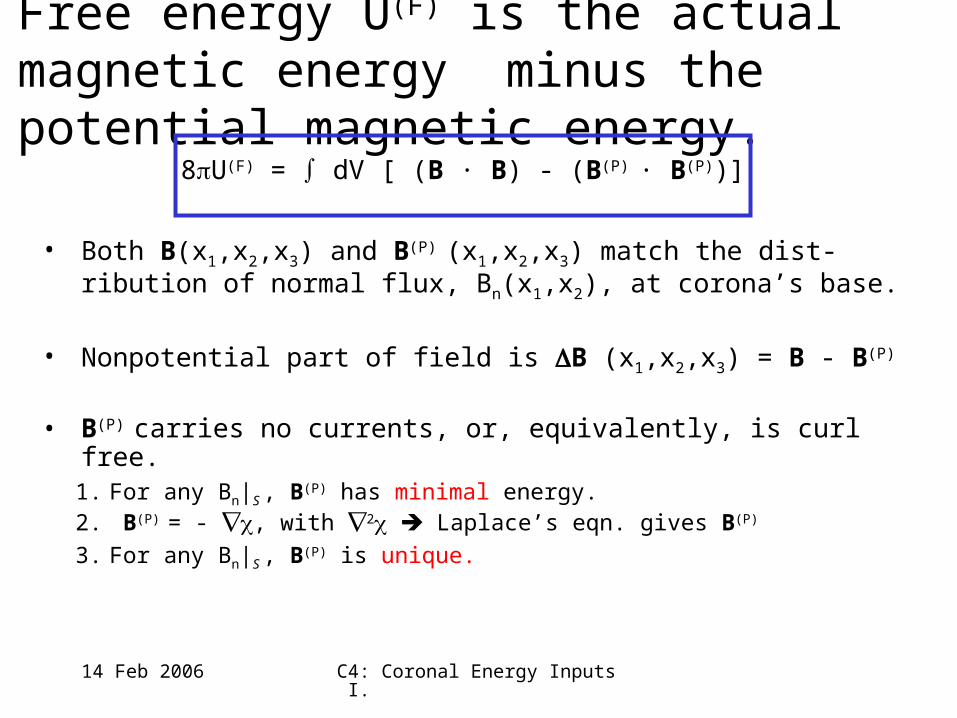
Free energy U(F) is the actual magnetic energy minus the potential magnetic energy.

8U(F) = dV [ (B · B) - (B(P) · B(P))]

• Both B(x1,x2,x3) and B(P) (x1,x2,x3) match the dist-ribution of normal flux, Bn(x1,x2), at corona’s base.

• Nonpotential part of field is B (x1,x2,x3) = B - B(P)

• B(P) carries no currents, or, equivalently, is curl free. 1. For any Bn|S , B(P) has minimal energy.2. B(P) = - , with 2 Laplace’s eqn. gives B(P)

3. For any Bn|S , B(P) is unique.


HMI data can be used in several ways to quantify free magnetic energy.

1. Use B(x1,x2,0) to extrapolate B & B(P) (McTiernan, Thurs. a.m.) – can compare model fields to AIA data

2. Magnetic Virial Theorem (Wheatland & Metcalf 2005) – novel application to photospheric magnetograms

3. Free Energy Flux (FEF) through photosphere (Welsch, 2006)– gives photospheric loci of energy injection

4. Magnetic charge topology (MCT, e.g., Barnes et al. 2005).– can give coronal loci of departures from potential field


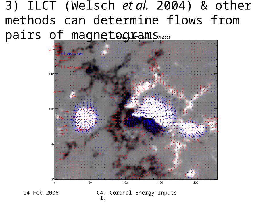
3) ILCT (Welsch et al. 2004) & other methods can determine flows from pairs of magnetograms.


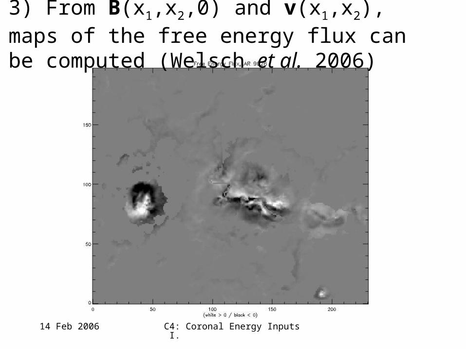
3) From B(x1,x2,0) and v(x1,x2), maps of the free energy flux can be computed (Welsch et al. 2006)


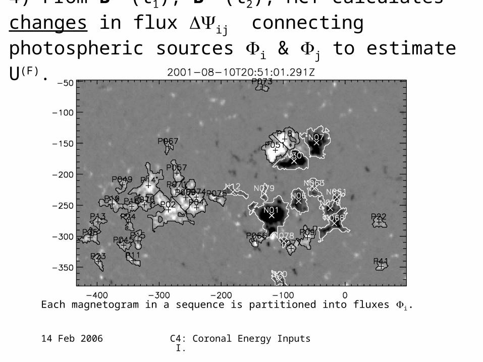
4) From B(P)(t1), B(P)(t2), MCT calculates changes in flux ij connecting photospheric sources i & j to estimate U(F).

Each magnetogram in a sequence is partitioned into fluxes i.


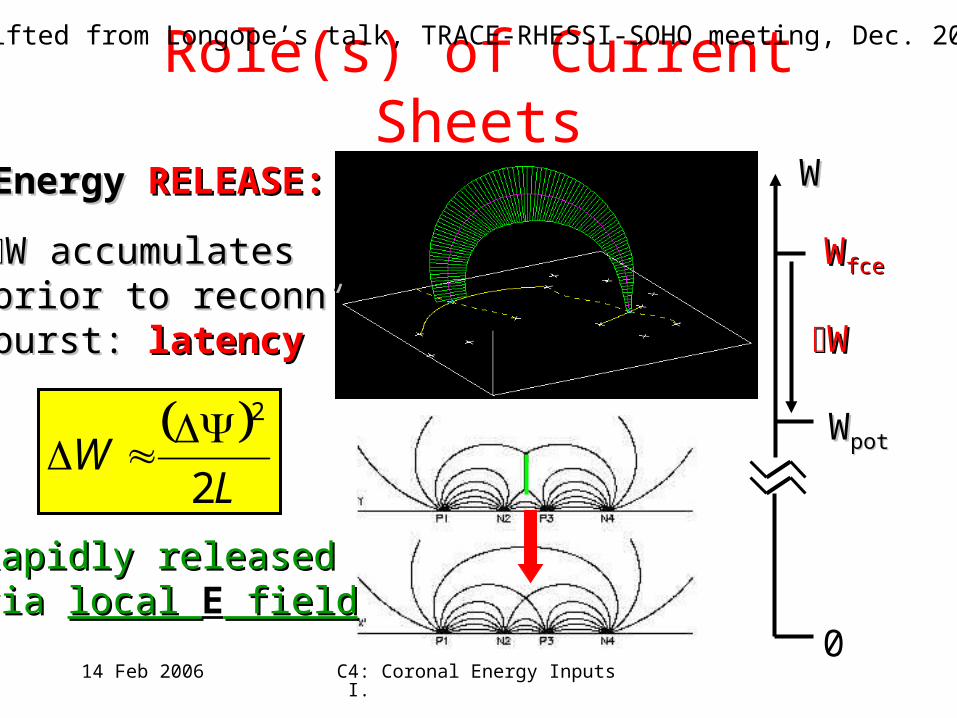
Role(s) of Current Sheets

0

WWfcefce

WWpotpot

WW

WW

Energy Energy RELEASE:RELEASE:

W accumulatesW accumulatesprior to reconn’prior to reconn’burst: burst: latencylatency

Rapidly releasedRapidly releasedvia via local local E field field

L

W2

2

4) [Lifted from Longope’s talk, TRACE-RHESSI-SOHO meeting, Dec. 2004]

L

W2

2


Here are a few random (and arguable!) thoughts that didn’t fit anywhere else.

• Mapping free energy using AIA data will require new techniques – not so with HMI.

• Techniques that can be automated would be good – AIA will generate a lot of data!

• AIA will tell us about non-potentiality from emergence – something HMI probably won’t do so well.


How can we use coronal observations to determine how much and where B differs from B(P)?

• Qualitative differences?– Canfield et al. (1999) – X-ray sigmoids– Schrijver, Title, & De Rosa (2005)


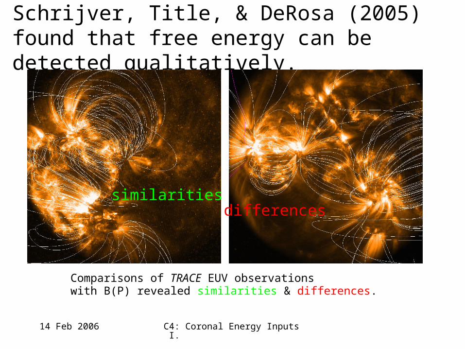
Schrijver, Title, & DeRosa (2005) found that free energy can be detected qualitatively.

Comparisons of TRACE EUV observationswith B(P) revealed similarities & differences.

similaritiesdifferences




• Quantitative differences?– Can we infer B directly?


Can we infer B directly from coronal morphology?

1. Gary & Alexander (1999) distorted of a model B to match coronal observations.

– assumed an initial topology in model B– distortions were non-force-free (but perhaps this is OK)

2. De Rosa (2004, unpublished?) investigated automated loop identification algorithms.

• Punchline: This is not easy to do!




• Quantitative differences?– Can we infer B directly?– If we cannot infer B, then what?

• Can we quantify departures from B(P)?


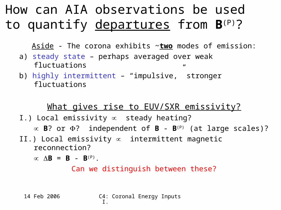
How can AIA observations be used to quantify departures from B(P)?

Aside - The corona exhibits ~two modes of emission:

a) steady state – perhaps averaged over weak fluctuations

b) highly intermittent – “impulsive,” stronger fluctuations

What gives rise to EUV/SXR emissivity?I.) Local emissivity steady heating?

B? or ? independent of B - B(P) (at large scales)?

II.) Local emissivity intermittent magnetic reconnection?

B = B - B(P).

Can we distinguish between these?


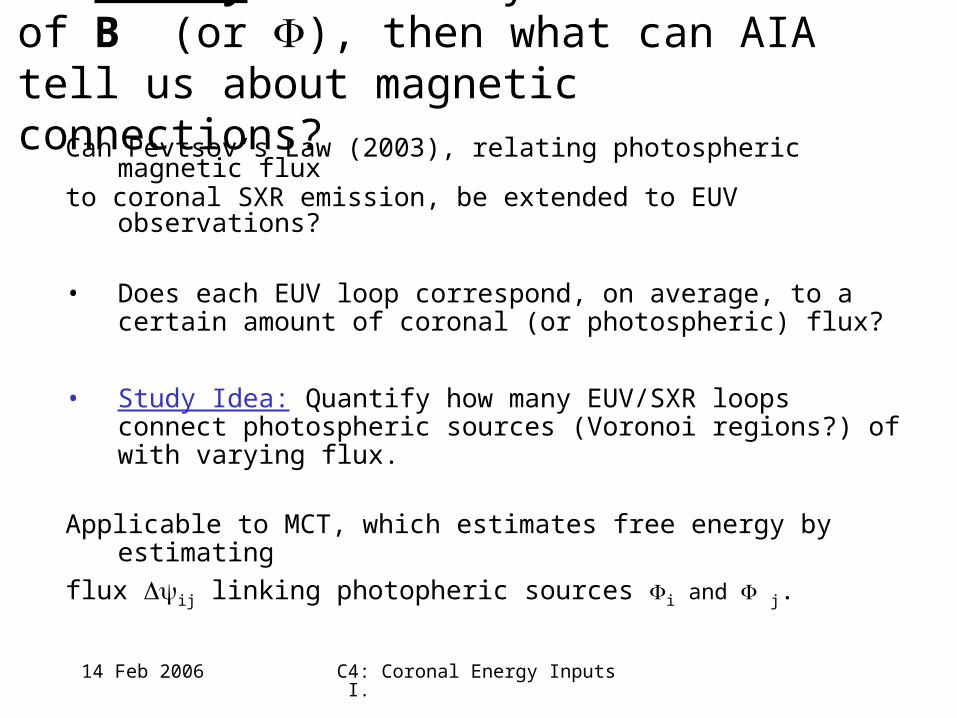
If steady emissivity is a function of B (or ), then what can AIA tell us about magnetic connections?

Can Pevtsov’s Law (2003), relating photospheric magnetic fluxto coronal SXR emission, be extended to EUV observations?

• Does each EUV loop correspond, on average, to a certain amount of coronal (or photospheric) flux?

• Study Idea: Quantify how many EUV/SXR loops connect photospheric sources (Voronoi regions?) of with varying flux.

Applicable to MCT, which estimates free energy by estimating

flux ij linking photopheric sources i and j.


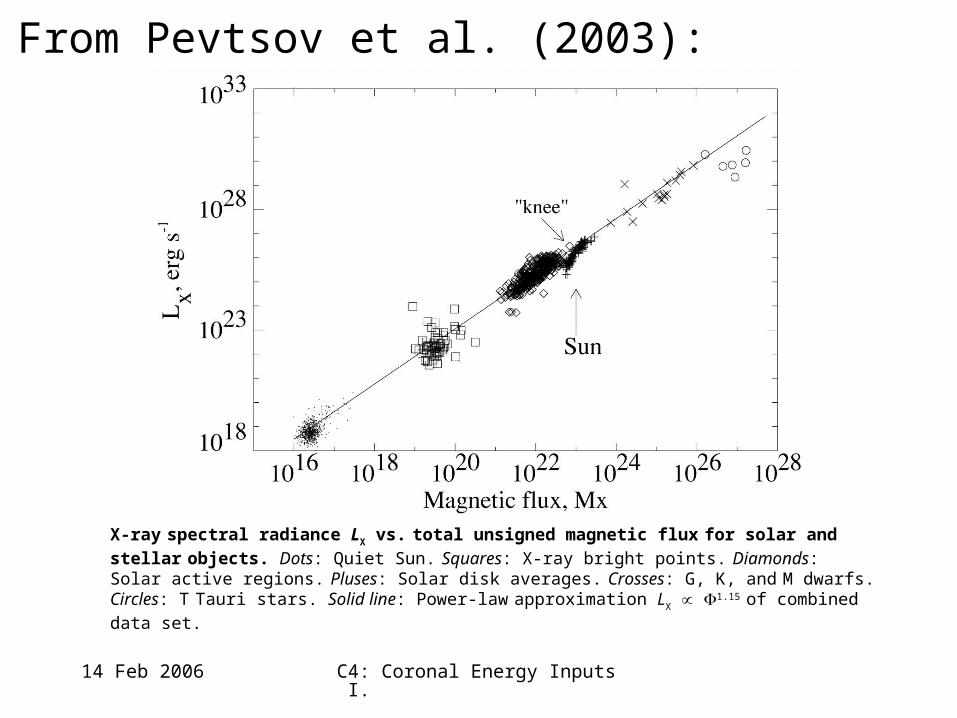
From Pevtsov et al. (2003):

X-ray spectral radiance LX vs. total unsigned magnetic flux for solar and stellar

objects. Dots: Quiet Sun. Squares: X-ray bright points. Diamonds: Solar active regions.

Pluses: Solar disk averages. Crosses: G, K, and M dwarfs. Circles: T Tauri stars. Solid line: Power-law approximation LX 1.15 of combined data set.


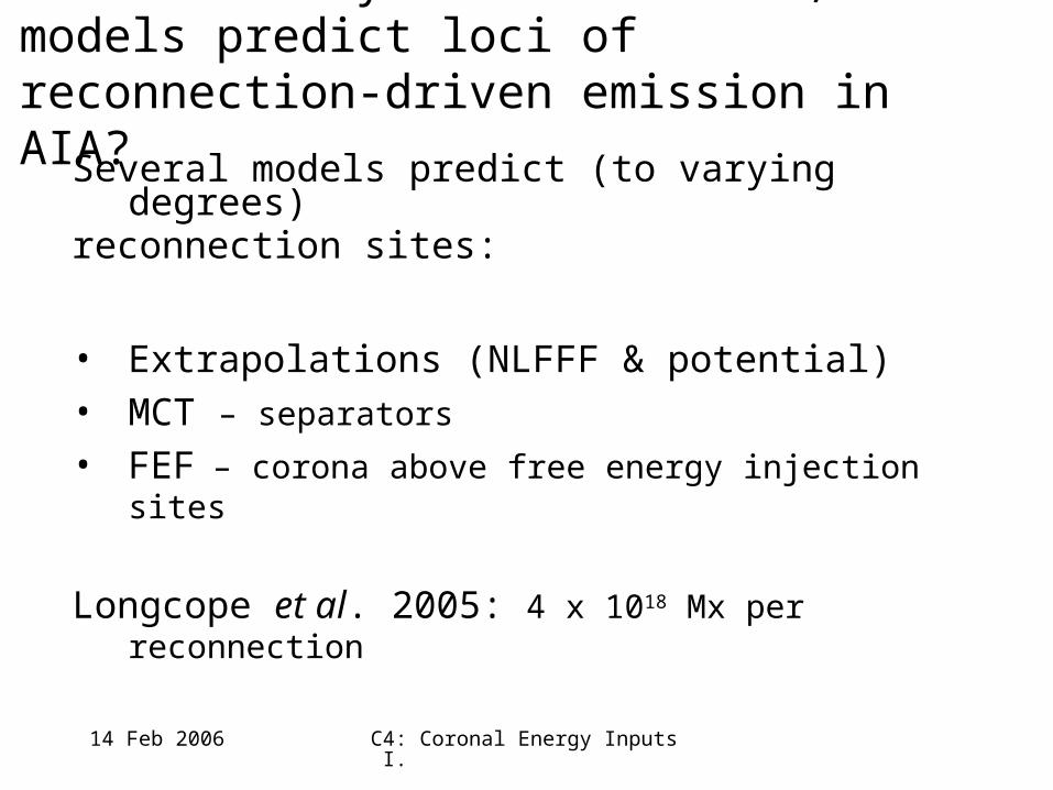
If emissivity B = B - B(P), can models predict loci of reconnection-driven emission in AIA?

Several models predict (to varying degrees)reconnection sites:

• Extrapolations (NLFFF & potential) • MCT – separators

• FEF – corona above free energy injection sites

Longcope et al. 2005: 4 x 1018 Mx per reconnection


Which observations might we pursue? A “starter” list:

1. Avg. reconnected flux, , per reconnection event?– avg. reconnected flux per DN?– avg. reconnected flux per coronal loop? (vs. ?)

2. Avg. reconnection rate, / t?3. Avg. “latency time” vs. spatial scale?

– Separatrices/ QSLs, during emergence are thin. Does this mean reconnection happens quickly? – How about during cancellations?– How about shear flows ?

4. What can we learn from “simulated emission” forward models? (Lundquist/Schrijver/Mok et al.’s)


References

• Barnes et al., 2005: Implementing a Magnetic Charge Topology Model for Solar Active Regions, Barnes, G., Longcope, D.W., & Leka, K.D., ApJ, v. 629, 561.

• Canfield et al. 1999: Sigmoidal morphology and eruptive solar activity, Canfield, R. C., Hudson, H.S., & McKenzie, D.E., GRL, v. 26, 627

• Démoulin & Berger, 2003: Magnetic Energy and Helicity Fluxes at the Photospheric Level, Démoulin, P., and Berger, M. A. Sol. Phys., v. 215, # 2, p. 203-215.

• Fletcher et al., 2003: Tracking of TRACE Ultraviolet Flare Footpoints, Fletcher, L., Pollock, J.A.., & Potts, H.E. Sol Phys, v. 222, 279

• Gary & Alexander, 1999: Constructing the Coronal Magnetic Field By Correlating Parameterized Magnetic Field Lines With Observed Coronal Plasma Structures, Gary, G.A., & Alexander, D., Sol Phys., v. 186, 123

• Longcope et al., 2005: Observations of Separator Reconnection to an Emerging Active Region, Longcope, D. W.; McKenzie, D. E.; Cirtain, J.; Scott, J. ApJ, v. 630, # 1, p. 596.

• Lundquist et al., 2005: Predicting Coronal Emissions with Multiple Heating Rates, Lundquist, L.L., Fisher, G.H., Leka, K.D., Metcalf, T.R., & McTiernan, J.M., AGU Spring Meeting Abstracts, A2

• Metcalf et al., 2005: Magnetic Free Energy in NOAA Active Region 10486 on 2003 October 29, Metcalf, T. R., Leka, K. D., Mickey, D. L., ApJ, 623, # 1, pp. L53-L56.

• Mok et al., 2005: Calculating the Thermal Structure of Solar Active Regions in Three Dimensions, Mok, Y., Miki\'c, Z., Lionello, R., & Linker, J.A., ApJ, v. 621, 1098


• Metcalf et al., 1995: Is the solar chromospheric magnetic field force-free? Metcalf, T. R., Jiao, L., McClymont, A. N., Canfield, R. C., Uitenbroek, H. , ApJ, v. 439, #1, p. 474- 481.

• Pevtsov et al., 2003:: The Relationship Between X-Ray Radiance and Magnetic Flux, Pevtsov, A.A., Fisher, G.H., Acton, L.W., Longcope, D.W., Johns-Krull, C.M., Kankelborg, C.C., & Metcalf, T.R., ApJ, v. 598, 1387.

• Schrijver et al., 2005: The Nonpotentiality of Active-Region Coronae and the Dynamics of the Photospheric Magnetic Field, Schrijver, C. J, DeRosa, M. L., Title, A. M., and Metcalf, T. R., ApJ, v. 628, #1, p. 501.

• Schrijver et al., 2004: The Coronal Heating Mechanism as Identified by Full-Sun Visualizations, Schrijver, C. J, Sandman, A. W.; Aschwanden, M. J., DeRosa, M. L., ApJ, v. 615, #1, p. 512.

• Welsch et al., 2004: ILCT: Recovering Photospheric Velocities from Magnetograms by Combining the Induction Equation with Local Correlation Tracking, Welsch, B. T., Fisher, G. H., Abbett, W.P., and Regnier, S., ApJ, v. 610, #2, p. 1148-1156.

• Welsch, 2006: Magnetic Flux Cancellation and Coronal Magnetic Energy, ApJ, in press.

• Wheatland et al., 2000: An Optimization Approach to Reconstructing Force-free Fields, Wheatland, M. S., Sturrock, P. A., Roumeliotis, ApJ, v. 540, #2, p. 1150-1155.

• Wheatland & Metcalf, 2005: An improved virial estimate of solar active region energy, Wheatland, M.S. and Metcalf, T.R. , ApJ, in press. (v. 636, #2, 10 Jan. 2006) [on astro-ph]

References, cont’d

Documents

Mapping Free Energy in the Solar Atmosphere