SOIL, 3, 191–210, 2017https://doi.org/10.5194/soil-3-191-2017© Author(s) 2017. This work is distributed underthe Creative Commons Attribution 3.0 License.

SOIL

Mapping of soil properties at high resolution inSwitzerland using boosted geoadditive models

Madlene Nussbaum1, Lorenz Walthert2, Marielle Fraefel2, Lucie Greiner3, and Andreas Papritz1

1Institute of Biogeochemistry and Pollutant Dynamics, ETH Zurich,Universitätstrasse 16, 8092 Zürich, Switzerland

2Swiss Federal Institute for Forest, Snow and Landscape Research (WSL),Zürcherstrasse 111, 8903 Birmensdorf, Switzerland

3Research Station Agroscope Reckenholz-Taenikon ART,Reckenholzstrasse 191, 8046 Zürich, Switzerland

Correspondence to: Madlene Nussbaum (madlene.nussbaum@env.ethz.ch)

Received: 7 April 2017 – Discussion started: 19 April 2017Revised: 11 September 2017 – Accepted: 7 October 2017 – Published: 16 November 2017

Abstract. High-resolution maps of soil properties are a prerequisite for assessing soil threats and soil functionsand for fostering the sustainable use of soil resources. For many regions in the world, accurate maps of soilproperties are missing, but often sparsely sampled (legacy) soil data are available. Soil property data (response)can then be related by digital soil mapping (DSM) to spatially exhaustive environmental data that describe soil-forming factors (covariates) to create spatially continuous maps. With airborne and space-borne remote sensingand multi-scale terrain analysis, large sets of covariates have become common. Building parsimonious modelsamenable to pedological interpretation is then a challenging task.

We propose a new boosted geoadditive modelling framework (geoGAM) for DSM. The geoGAM modelssmooth non-linear relations between responses and single covariates and combines these model terms additively.Residual spatial autocorrelation is captured by a smooth function of spatial coordinates, and non-stationaryeffects are included through interactions between covariates and smooth spatial functions. The core of fullyautomated model building for geoGAM is component-wise gradient boosting.

We illustrate the application of the geoGAM framework by using soil data from the Canton of Zurich, Switzer-land. We modelled effective cation exchange capacity (ECEC) in forest topsoils as a continuous response. Foragricultural land we predicted the presence of waterlogged horizons in given soil depths as binary and drainageclasses as ordinal responses. For the latter we used proportional odds geoGAM, taking the ordering of the re-sponse properly into account. Fitted geoGAM contained only a few covariates (7 to 17) selected from large sets(333 covariates for forests, 498 for agricultural land). Model sparsity allowed for covariate interpretation throughpartial effects plots. Prediction intervals were computed by model-based bootstrapping for ECEC. The predictiveperformance of the fitted geoGAM, tested with independent validation data and specific skill scores for contin-uous, binary and ordinal responses, compared well with other studies that modelled similar soil properties. Skillscore (SS) values of 0.23 to 0.53 (with SS= 1 for perfect predictions and SS= 0 for zero explained variance)were achieved depending on the response and type of score. GeoGAM combines efficient model building fromlarge sets of covariates with effects that are easy to interpret and therefore likely raises the acceptance of DSMproducts by end-users.

Published by Copernicus Publications on behalf of the European Geosciences Union.

192 M. Nussbaum et al.: Soil mapping using boosted geoadditive models

1 Introduction

Soils fulfil many functions important for agriculture, forestryand the management of soil resources and natural hazards.The functionality of soils depends on their properties; hence,accurate and spatially highly resolved maps of basic soilproperties such as texture, organic carbon content and pHfor specific soil depth are needed for the sustainable man-agement of soils (FAO and ITPS, 2015). Unfortunately, suchsoil property maps are often missing and the availability ofsoil information is very different between nations and conti-nents (Omuto and Nachtergaele, 2013). For areas where spa-tially referenced but sparse (legacy) soil data are available,e.g. soil datasets consisting of soil profile data and labora-tory measurements, these point data can be linked using dig-ital soil mapping (DSM) techniques (e.g. McBratney et al.,2003; Scull et al., 2003) to spatial information on soil forma-tion factors to generate spatially continuous maps.

In the past, many DSM approaches have been proposedto exploit the correlation between soil properties (responseY (s)) and soil-forming factors (covariates x(s)). Linear re-gression modelling (LM; e.g. Meersmans et al., 2008; Henglet al., 2014) and kriging with external drift (EDK), its ex-tension for autocorrelated errors (Bourennane et al., 1996;Nussbaum et al., 2014), have often been used. The strengthof LM and EDK is the ease of interpretation of the fittedmodels (e.g. through partial residual plots; Faraway, 2005,p. 73). This is important for checking whether modelled re-lations between the target soil property and soil-forming fac-tors accord with pedological expertise and for conveying theresults of DSM analyses to users of such products. LM andEDK capture only linear relations between the covariates anda response. By using interactions between covariates, onecan sometimes account for non-linear relationships, but thisquickly becomes unwieldy for a large number of covariates(e.g. above 30). Fitting models to (very) large sets of covari-ates has become common with the advent of remotely senseddata (Ben-Dor et al., 2009; Mulder et al., 2011) and novelapproaches for terrain analysis (Behrens et al., 2010). Modelbuilding, i.e. covariate selection, is then a formidable task.Although specialised methods like L2-boosting (Bühlmannand Hothorn, 2007) and lasso (least absolute shrinkage andselection operator; Hastie et al., 2009, Chap. 3) are available,they have not often been used for DSM (Nussbaum et al.,2014; Liddicoat et al., 2015; Fitzpatrick et al., 2016). Gener-alised linear models (GLMs; e.g. Dobson, 2002) extend lin-ear modelling to binary, nominal (e.g. soil taxonomic units;Hengl et al., 2014; Heung et al., 2016) or ordinal responses(e.g. soil drainage classes; Campling et al., 2002). AlthoughGLMs are non-linear models, the non-linearly transformedconditional expectation g(E[Y (s)|x(s)]), where g(·) is someknown link function, still depends linearly on covariates.

Lately, tree-based machine learning methods have be-come popular for DSM. Classification and regression trees(CARTs; e.g. Liess et al., 2012; Heung et al., 2016), Cubist

(e.g. Henderson et al., 2005; Adhikari et al., 2013; Lacosteet al., 2016) and ensemble tree methods like random forest(RF; e.g. Grimm et al., 2008; Wiesmeier et al., 2011) andboosted regression trees (BRTs; e.g. Moran and Bui, 2002;Martin et al., 2011) have been used.

All tree-based methods easily account for complex non-linear relations between responses and covariates. Theymodel continuous and categorical responses (albeit withoutmaking a difference between nominal and ordinal responses),inherently deal with incomplete covariate data and allow forthe modelling of spatially changing (non-stationary) relation-ships. BRT and RF fit models to large sets of covariates. Thestructure of the fitted models can be explored with variableimportance and partial dependence plots (Hastie et al., 2009,Sect. 10.9, and for an application Martin et al., 2011). Never-theless, tree-based ensemble methods remain complex, andresults are not as easy to interpret regarding the relevant soil-forming factors resulting from (G)LM.

Generalised additive models (GAMs; e.g. Hastie and Tib-shirani, 1990, Chap. 6) offer a compromise between ease ofinterpretation and flexibility in modelling non-linear relation-ships. GAMs expand the (possibly transformed) conditionalexpectation of a response given covariates as an additive se-ries:

g(

E[Y (s) |x(s)

])= ν+ f

(x(s)

)= ν+

∑j

fj(xj (s)

), (1)

where ν is a constant, and fj(xj (s)

)values are linear terms or

unspecified “smooth” non-linear functions of single covari-ates xj (s) (e.g. smoothing spline, kernel or any other scatterplot smoother) and g(·) is again a link function. GAMs ex-tend GLMs to account for truly non-linear relations betweenY and x (and not just for non-linearities imposed by g), butthey limit the complexity of the fitted functions to additivecombinations of simple non-linear terms and thereby avoidthe curse of dimensionality (Hastie et al., 2009, Sect. 2.5).For continuous, ordinal and nominal responses, GAMs canbe readily fitted to large sets of covariates through boost-ing (Hofner et al., 2014; Hothorn et al., 2015). Boostinghandles covariate selection and avoids over-fitting if stoppedearly (Bühlmann and Hothorn, 2007). Hence, the structure ofboosted GAMs can be more easily checked and interpretedthan RF and BRT models. In the past, GAMs have occasion-ally been used for DSM and only recently became more pop-ular (e.g. Buchanan et al., 2012; Poggio et al., 2013; Poggioand Gimona, 2014; de Brogniez et al., 2015; Sindayiheburaet al., 2017).

Besides accurate predictions, accurate modelling of pre-diction uncertainty sometimes also matters for DSM (e.g. formapping temporal changes in soil carbon and nutrientsstocks). Quantile regression forest (Meinshausen, 2006), anextension of RF, estimates the quantiles of the distributionsY (s)|x(s) and provides prediction intervals directly. Predic-tion intervals can also easily be constructed for predictionsby EDK, (G)LM and GAM, as long as the uncertainty arising

SOIL, 3, 191–210, 2017 www.soil-journal.net/3/191/2017/

M. Nussbaum et al.: Soil mapping using boosted geoadditive models 193

from model building is ignored. To take the effect of modelbuilding properly into account one resorts best to bootstrap-ping (Davison and Hinkley, 1997, Sect. 6.3.3). Bootstrappingis also useful to model prediction uncertainty for boostedmodels, which do not qualify the accuracy of predictionsper se, and to account for all sources of prediction un-certainty in regression kriging approaches (Viscarra Rosselet al., 2014).

In summary, a versatile DSM procedure should

1. model non-linear relations between Y (s) and x(s), whereresponses and covariates may be continuous, binary,nominal or ordinal variables,

2. efficiently build models with good predictive perfor-mance for large sets of covariates (p>>30),

3. preferably result in parsimonious models with a simplestructure that can be easily interpreted and checked forplausibility, and

4. accurately quantify the accuracy of predictions com-puted from the fitted models.

The objective of our work was to develop a DSM frame-work that meets requirements 1–4 based on boosted geoad-ditive models (geoGAMs), an extension of GAM for spatialdata. First, we introduce the modelling framework and de-scribe in detail the model-building procedure. Second, weuse the method in three DSM case studies in the Canton ofZurich, Switzerland that aim at different types of responses:effective cation exchange capacity (ECEC) of forest topsoils(continuous response), the presence or absence of morpho-logical features for waterlogging in agricultural soils (binaryresponse) and drainage classes characterising the prevalenceof anoxic conditions, again in agricultural soils (ordinal re-sponse). To assess the validity of the modelling results withindependent data (obtained by splitting the original datasetinto calibration and validations subsets), we used specific cri-teria that take the nature of the various responses properlyinto account. These criteria are in common use for forecastverification in atmospheric sciences (e.g. Wilks, 2011), but toour knowledge have not often been used to (cross-)validateDSM predictions.

2 The geoGAM framework

2.1 Model representation

A generalised additive model (GAM) is based on the fol-lowing components (Hastie and Tibshirani, 1990, Chap. 6and Eq. 1). (i) Response distribution: given x(s)=(x1(s),x2(s), . . . ,xp(s)

)T, the Y (s) values are conditionallyindependent observations from simple exponential familydistributions. (ii) Link function: g(·) relates the expectationµ(x(s)

)= E

[Y (s)|x(s)

]of the response distribution to (iii)

the additive predictor∑jfj

(xj (s)

).

GeoGAM extends GAM by allowing for a more complexform of the additive predictor (Kneib et al., 2009; Hothornet al., 2011). First, one can add a smooth function fs(s) ofthe spatial coordinates (smooth spatial surface) to the addi-tive predictor to account for residual autocorrelation. Morecomplex relationships between Y and x can be modelled byadding terms like fj

(xj (s)

)· fk

(xk(s)

)to capture the effect

of interactions between covariates and fs(s) ·fj(xj (s)

)to ac-

count for the spatially changing dependence between Y andx. Hence, in its full generality, a generalised additive modelfor spatial data is represented by

g(µ(x(s)

))= ν+ f

(x(s)

)= ν+

∑u

fju(xju (s)

)+

∑v

fjv(xjv (s)

)· fkv

(xkv (s)

)︸ ︷︷ ︸

global marginal and interaction effects

+

∑w

fsw (s) · fjw(xjw (s)

)︸ ︷︷ ︸

non-stationary effects

+ fs(s)︸︷︷︸autocorrelation

. (2)

Kneib et al. (2009) called Eq. (2) a geoadditive model, aname coined before by Kammann and Wand (2003) for acombination of Eq. (1) with a geostatistical error model.

It remains to be specified what response distributions andlink functions should be used for the various response types.For (possibly transformed) continuous responses, one oftenuses a normal response distribution combined with the iden-tity link g

(µ(x(s))

)= µ

(x(s)

). For binary data (coded as 0

and 1), one assumes a Bernoulli distribution and often uses alogit link:

g (µ (x (s)))= log(

µ (x (s))1−µ (x (s))

), (3)

where

µ(x(s)

)= Prob

[Y (s)= 1 |x(s)

]=

exp(ν+ f

(x(s)

))1+ exp

(ν+ f

(x(s)

)) . (4)

For ordinal data with ordered response levels, 1,2, . . . ,k,we used the cumulative logit or proportional odds model(Tutz, 2012, Sect. 9.1). For any given level r ∈ (1,2, . . . ,k),the logarithm of the odds of the event Y (s)≤ r |x(s) is thenmodelled by

log

(Prob

[Y (s)≤ r |x(s)

]Prob

[Y (s)> r |x(s)

])= νr + f (x(s)), (5)

with νr a sequence of level-specific constants satisfying ν1 ≤

ν2 ≤ . . .≤ νr . Conversely,

Prob[Y (s)≤ r |x(s)

]=

exp(νr + f

(x(s)

))1+ exp

(νr + f

(x(s)

)) . (6)

Note that Prob[Y (s)≤ r |x(s)

]depends on r only through the

constant νr . Hence, the ratio of the odds of two events Y (s)≤r |x(s) and Y (s)≤ r | x(s) is the same for all r (Tutz, 2012,p. 245).

www.soil-journal.net/3/191/2017/ SOIL, 3, 191–210, 2017

194 M. Nussbaum et al.: Soil mapping using boosted geoadditive models

2.2 Model building (selection of covariates)

To build parsimonious models that can readily be checkedfor agreement with pedological understanding, we applied asequence of fully automated steps 1–6. In several of thesesteps we optimised tuning parameters through 10-fold cross-validation with fixed subsets using root mean square error(RMSE; Eq. (12), continuous responses), Brier score (BS;Eq. (16), binary responses) or ranked probability score (RPS;Eq. (18), ordinal responses) as optimisation criteria. Modelbuilding aims to optimise the accuracy of predictions, andhence we did not use equivalent “goodness-of-fit” statistics.To improve the stability of the algorithm continuous covari-ates were first scaled (by the difference of the maximum andminimum value) and centred.

1. Boosting (see step 2 below) is more stable and con-verges more quickly when the effects of categorical co-variates (factors) are accounted for as a model offset.We therefore used the group lasso (Breheny and Huang,2015) – an algorithm that likely excludes non-relevantcovariates and treats factors as groups – to select impor-tant factors for the offset. For ordinal responses (Eq. 6)we used stepwise proportional odds logistic regressionin both directions with BIC (e.g. Faraway, 2005, p. 126)to select the offset covariates because lasso cannot beused for such responses.

2. Next, we selected a subset of relevant factors, continu-ous covariates and spatial effects by using component-wise gradient boosting. Boosting is a slow stage-wiseadditive learning algorithm. It expands f

(x(s)

)in a set

of base procedures (base learners) and approximates theadditive predictor by using a finite sum of them as fol-lows (Bühlmann and Hothorn, 2007).

(a) Initialise f(x(s)

)[m] with the offset of step 1 aboveand set m= 0.

(b) Increase m by 1. Compute the negative gradientvector U[m] (e.g. residuals) for a loss function l(·).

(c) Fit all base learners fj(xj (s)

),j = 1, . . . ,p to

U[m] and select the base learner, for examplefk(xk(s))[m], that minimizes l(·).

(d) Update f(x(s)

)[m]= f

(x(s)

)[m−1]+v ·fk

(xk(s)

)[m]with step size v ≤ 1.

(e) Iterate steps (b) to (d) until m=mstop (main tuningparameter).

We used the following settings in the above algorithm.As loss functions l(·) we used L2 for continuous, neg-ative binomial likelihood for binary (Bühlmann andHothorn, 2007) and proportional odds likelihood for or-dinal responses (Schmid et al., 2011). Early stoppingof the boosting algorithm was achieved by determiningoptimalmstop through cross-validation. We used default

step length (υ = 0.1). This is not a sensitive parameteras long as it is clearly below 1 (Hofner et al., 2014).For continuous covariates we used penalised smoothingspline base learners (Kneib et al., 2009). Factors weretreated as linear base learners. To capture residual auto-correlation we added a bivariate tensor product P-splineof spatial coordinates (Wood, 2006, pp. 162) to the ad-ditive predictor. Spatially varying effects were modelledby using base learners formed through multiplication ofcontinuous covariates with tensor product P-splines ofspatial coordinates (Wood, 2006, pp. 168). An unevendegree of freedom of base learners biases base learnerselection (Hofner et al., 2011). We therefore penalisedeach base learner to 5 degrees of freedom (df). Factorswith fewer than six levels (df< 5) were aggregated togrouped base learners. By using an offset, the effects ofimportant factors with more than six levels were implic-itly accounted for without penalisation.

3. Atmstop (see step 2 above), many included base learnershad very small effects only. We fitted generalised addi-tive models (GAMs; Wood, 2011) and included smoothand factor effects only if their effect size ej of the cor-responding base learner fj (xj (s)) was substantial. Theeffect size ej of factors was the largest difference be-tween the effects of two levels and for continuous co-variates it was equal to the maximum contrast of esti-mated partial effects (after the removal of extreme val-ues as in box plots; Frigge et al., 1989). We iteratedthrough ej and excluded covariates with ej smaller thana threshold effect size et . Optimal et was determined by10-fold cross-validation of GAM. In these GAM fits,smooth effects were penalised by 5 degrees of free-dom as imposed by component-wise gradient boosting(step 2 above). The factors selected as an offset in step1 were now included in the GAM.

4. We further reduced the GAM through the stepwiseremoval of covariates by using cross-validation. Thecandidate covariate to drop was chosen by the largestp value of F tests for linear terms and approximateF tests (Wood, 2011) for smooth terms.

5. Factor levels with similar estimated effects were mergedstepwise again through cross-validation based on thelargest p values from two sample t tests of partial resid-uals.

6. The final model (used to compute spatial predictions)was a parsimonious GAM. Because of step 5, factorspossibly had a reduced number of coefficients. The ef-fects of continuous covariates were modelled by smoothfunctions and – if at all present – spatially structuredresidual variation (autocorrelation) was represented by asmooth spatial surface. To avoid over-fitting, both typesof smooth effects were penalised by 5 degrees of free-dom (as imposed in step 2).

SOIL, 3, 191–210, 2017 www.soil-journal.net/3/191/2017/

M. Nussbaum et al.: Soil mapping using boosted geoadditive models 195

Model-building steps 1 to 6 were implemented in the Rpackage geoGAM (Nussbaum, 2017).

2.3 Predictions and predictive distribution

Soil properties were predicted for new locations s+ fromthe final geoGAM by using Y (s+)= f

(x(s+)

). To model the

predictive distributions for continuous responses we used anon-parametric, model-based bootstrapping approach (Davi-son and Hinkley, 1997, pp. 262, 285) as follows.

A. New values of the response were simulated according toY (s)∗ = f

(x(s)

)+ε, where f

(x(s)

)represents the fitted

values of the final model and ε values are errors ran-domly sampled with replacement from the centred, ho-moscedastic residuals of the final model (Wood, 2006,p. 129).

B. The geoGAM was fitted to Y (s)∗ according to steps 1–6of Sect. 2.2.

C. Prediction errors were computed according to δ∗+ =

f(x(s+)

)∗−

(f(x(s+)

)+ ε

), where f (x(s+))∗ repre-

sents predicted values at new locations s+ of the modelbuilt with the simulated response Y (s)∗ in step B above,and the errors ε are again randomly sampled from thecentred, homoscedastic residuals of the final model (seestep A).

Prediction intervals were computed according to[f(x(s+)

)− δ∗+ (1−α) ; f

(x(s+)

)− δ∗+ (α)

], (7)

where δ∗+ (α) and δ∗

+ (1−α) are the α and (1−α) quantiles ofδ∗+ pooled over all 1000 bootstrap repetitions.

Predictive distributions for binary and ordinal responseswere directly obtained from the final geoGAM fit by predict-ing probabilities of occurrence Prob

(Y (s)= r |x(s)

)(Davi-

son and Hinkley, 1997, p. 358).

3 Case studies: materials and methods

3.1 Study regions

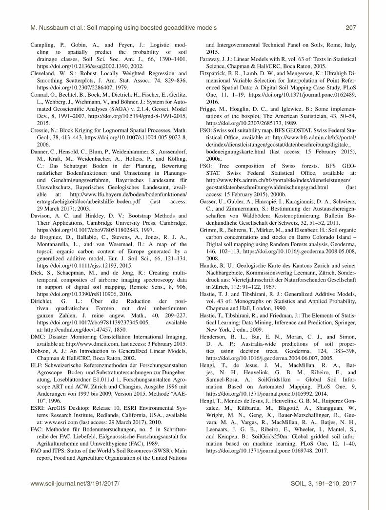
We applied the modelling framework to three datasets onproperties of forest and agricultural soils in the Canton ofZurich in Switzerland (Fig. 1). Forests (ZH forest), as definedby the Swiss topographic landscape model (swissTLM3D,Swisstopo, 2013a), cover an area of 506.5 km2, or roughly30 % of the total area of the Canton of Zurich. The spatialextent of the agricultural region near Greifensee was definedby the availability of imaging spectroscopy data collected bythe APEX spectrometer (Schaepman et al., 2015). Agricul-tural land was defined as the area not covered by any arealfeatures, such as settlements or forests, extracted from theSwiss topographic landscape model (swissTLM3D, Swis-stopo, 2013a). Wetlands, forests, parks or city gardens wereexcluded, resulting in a study region of 170 km2.

0 50 100 km

Data sources: Biogeographical regions © 2001 BAFU / Swiss Boundary, Lakes ©2012 BFS GEOSTAT / Boundries Europe: NUTS © 2010 EuroGeographics

Jura

Alps

Greifensee

Plateau

ZH forest

Figure 1. Location of the study regions Greifensee and ZH foreston the Swiss Plateau.

In the Canton of Zurich, forests extend across altitudesranging from 340 to 1170 m above sea level (m. a.s.l), and inthe Greifensee area elevation ranges from 390 to 840 m a.s.l.(Swisstopo, 2016). The climatic conditions (period 1961–1990; Zimmermann and Kienast, 1999) vary accordingly,with mean annual rainfall of 880–1780 mm for the forestedand 1040–1590 mm for the agricultural study region. Meanannual temperatures range between 6.1–9.1 and 7.5–9.1 ◦C,respectively. Two-thirds of the forested area is dominated byconiferous trees (FSO, 2000b). Half of the Greifensee studyregion is covered by cropland and one-third by permanentgrassland. The remainder is comprised of orchards, horti-cultural areas or mountain pastures (Hotz et al., 2005). Inthe Canton of Zurich, soils are formed mostly from Molasseformations and Quaternary sediments dominantly from thelast glaciation (Würm). In the north-eastern part, the lime-stone Jura hills reach into the ZH forest study region (Hantke,1967).

3.2 Data

3.2.1 Soil database

We used legacy soil data collected between 1985 and 2014.Data originate from long-term soil monitoring of the Cantonof Zurich (KaBo), a soil pollutant survey (Wegelin, 1989),field surveys for creating soil maps of the agricultural land(Jäggli et al., 1998) or soil investigations in the course ofdifferent projects by the Swiss Federal Institute for Forest,Snow and Landscape Research (WSL; Walthert et al., 2004).Sites for pollutant surveying were chosen on a regular grid,and those for creating soil maps were determined throughpurposive sampling (Webster and Lark, 2013, p. 86) by fieldsurveyors to best represent the soils typical for the givenlandform. The sites of WSL were chosen through purposive

www.soil-journal.net/3/191/2017/ SOIL, 3, 191–210, 2017

196 M. Nussbaum et al.: Soil mapping using boosted geoadditive models

sampling according to the aims of the project. Soil data weretherefore quite heterogeneous, and tailored harmonisationprocedures were required to provide consistent soil datasets.The heterogeneity resulted from several standards of soil de-scription and soil classification, different data keys, differentanalytical methods and, in particular, often missing metadatafor a proper interpretation of the datasets. Therefore, we elab-orated a general harmonisation scheme that covers the mainsteps required to merge different soil legacy data into onecommon, consistent database (Walthert et al., 2016). Sam-pling sites were recorded in the field on topographic maps(scale 1 : 25 000), and hence we estimated the accuracy ofcoordinates to about ±25 m.

3.2.2 Effective cation exchange capacity (ECEC, forestsoils)

After the removal of sites with missing covariate values, weused 1844 topsoil samples from 1348 sites with data on effec-tive cation exchange capacity (ECEC). Most measurementsrefer to composite samples for which aliquots were measuredin 20 m× 20 m squares from 0–20 cm of soil depth. For about100 sites, soil profile genetic horizons were sampled. ECEC[mmolc kg−1] for 0–20 cm was computed from horizon databy using

ECEC0−20 =

h∑i=1

wiECECi, (8)

where ECECi is the value for horizon i, wi is a weight givenby soil density ρi and the fraction of the thickness of horizoni within 0–20 cm and h is the number of horizons intersect-ing the 0–20 cm depth; ρi was estimated from soil organicmatter (SOM) and/or sampling depth by using a pedotrans-fer function (PTF; see the Supplement of Nussbaum et al.,2017). Due to a lack of respective data, the volumetric stonecontent was assumed to be constant.

For most soil samples, ECEC was measured after extrac-tion in an ammonium chloride solution (FAC, 1989; Walthertet al., 2004, 2013). Roughly 5 % of the samples had onlymeasurements of Ca, Mg, K and Al (extracted by ammo-nium acetate EDTA solution; Lakanen and Erviö, 1971; ELF,1996; Gasser et al., 2011). For these samples, we estimatedECEC by using a PTF (Nussbaum and Papritz, 2015).

We assigned 293 of 1348 sites (528 samples) to the valida-tion set, which was used to check the predictive performanceof the fitted statistical model, and the remaining 1055 sites(1316 samples) were used to calibrate the model. The legacysamples were spatially clustered. To ensure that the valida-tion sites were evenly spread over the study region, the vali-dation sites were selected by weighted random sampling. Theweight attributed to a site was proportional to the forestedarea within its Dirichlet polygon (Dirichlet, 1850).

We found a considerable variation in ECEC values rangingfrom 17.4 to 780 mmolc kg−1 (median 141.1 mmolc kg−1;

Table S1 in the Supplement). On average, ECEC was slightlylarger in the calibration than in the validation set.

3.2.3 Presence of waterlogged soil horizons(agricultural soils)

Waterlogging characteristics were recorded in the field at 962sites within the Greifensee study region by visual evaluation(Jäggli et al., 1998). Swiss soil classification distinguisheshorizon qualifiers gg (strongly gleyic, predominantly oxi-dised) and r (anoxic, predominantly reduced) and both arebelieved to limit plant growth (Jäggli et al., 1998; Mülleret al., 2007; Litz, 1998; Danner et al., 2003; Kreuzwieser andRennberg, 2014).

We constructed binary responses for three soil depths: 0–30 cm, 0–50 cm and 0–100 cm. If one of the horizon quali-fiers gg or r was recorded within the interval, we assigned 1as the presence of waterlogged horizons and 0 as the absenceof waterlogged soil horizons otherwise.

We chose 198 of 962 sites to form a validation set, againby using weighted random sampling. The remaining 764sites were used to build and fit the models. In the topsoil(0–30 cm), gg or r horizon qualifiers were only observed at13.4 % of the 962 sites. Down to 50 cm, about twice as manysites (25.9 %) showed signs of anoxic conditions and downto 1 m 38.6 % of sites featured an anoxic or gleyic horizon(Table S2).

3.2.4 Drainage classes (agricultural soils)

Swiss soil classification differentiates the hydromorphic fea-tures of soils in more detail, describing the degree, depth andsource of waterlogging with three supplementary qualifiersfor stagnic, gleyic or anoxic profiles (I, G, R; categorical at-tributes, Brunner et al., 1997). To reduce the complexity ofclassification, we aggregated these qualifiers to three orderedlevels: well drained (qualifiers I1–I2, G1–G3, R1 or no hy-dromorphic qualifier), moderately well drained (I3–I4, G4)and poorly drained (G5–G6, R2–R5).

For validation we used the same 198 sites as for thepresence of waterlogged soil horizons, but only 732 siteswere used for model building due to missing supplemen-tary qualifiers. The majority (66.6 %) of the 930 sites werewell drained, only 12.7 % were classified as moderately welldrained and 20.7 % as poorly drained (Table S3 in the Sup-plement).

3.2.5 Covariates for statistical modelling

To represent local soil formation conditions, we used datafrom 23 sources (Table 1). For ECEC a total of 333 covari-ates were used to describe climatic (71 covariates) and topo-graphic conditions (196 covariates). For the agricultural land,we additionally used 180 spectral bands of the APEX spec-trometer, spatial information on historic wetlands and agri-

SOIL, 3, 191–210, 2017 www.soil-journal.net/3/191/2017/

M. Nussbaum et al.: Soil mapping using boosted geoadditive models 197

cultural drainage networks, resulting in 498 covariates in to-tal.

3.3 Statistical analysis

We built models for the five responses according to Sect. 2.2and computed predictions for new locations at nodes of a20 m grid. Predictions were post-processed as described inthe following.

3.3.1 Response transformation

ECEC data for 0–20 cm of soil depth were positively skewed(Table S1); hence we fitted the model to the log-transformeddata. In full analogy to log-normal kriging (Cressie, 2006,Eq. 20), the predictions were back-transformed by using

E[Y (s+) |x

]= exp

(f(x(s+)

)+

12σ 2−

12

Var[f(x(s+)

)]),

(9)

with f(x(s+)

)being the prediction of the log-transformed

response, σ 2 the estimated residual variance of the final ge-oGAM fit and Var

[f(x(s+)

)]the variance of f

(x(s+)

)as

provided by the final geoGAM. Limits of prediction intervalswere back-transformed by using exp(·) as they are quantilesof the predictive distributions.

3.3.2 Conversion of probabilistic to categoricalpredictions

For binary and ordinal responses, Eqs. (4) and (6) predictprobabilities of the respective response levels. To predict the“most likely” outcome one has to apply a threshold to theseprobabilities. For binary data we predicted the presence ofwaterlogged horizons if the probability exceeded the optimalvalue of the Gilbert skill score (GSS; Sect. 3.3.3) that dis-criminated between the presence and absence of waterloggedhorizons best in cross-validation of the final geoGAM. GSSwas selected because the absence of waterlogged horizonswas more common than presence, especially in topsoil. Toensure consistency in the maps for sequential soil depths weassigned the presence of waterlogged horizons to the lowerdepth if it was predicted for the depth above.

For ordinal responses we predicted the level to which themedian of the probability distribution Prob(Y (s)≤ r|x(s))was assigned (Tutz, 2012, p. 475).

3.3.3 Evaluating the predictive performance of thestatistical models

The predictive performance of the geoGAM, fitted for thecontinuous response ECEC, was tested by comparing predic-tions Y (si) (Eq. 9) with measurements Y (si) of independent

validation sets. Marginal bias and overall accuracy were as-sessed by using

BIAS=−1n

n∑i=1

(Y (si)− Y (si)), (10)

robBIAS=−median1≤i≤n(Y (si)− Y (si)

), (11)

RMSE=

(1n

n∑i=1

(Y (si)− Y (si)

)2)1/2

, (12)

robRMSE=MAD1≤i≤n(Y (si)− Y (si)

), (13)

SSmse = 1−

∑ni=1

(Y (si)− Y (si)

)2∑ni=1

(Y (si)− 1

n

∑ni=1Y (si)

)2 , (14)

where MAD is the median absolute deviation. SSmse was de-fined as mean square error skill score (Wilks, 2011, p. 359)with the sample mean of the measurements as a refer-ence prediction method. Interpretation is similar to R2 withSSmse = 1 for perfect predictions and SSmse = 0 for zeroexplained variance. SSmse becomes negative if the root meansquare error (RMSE) exceeds the standard deviation of thedata. To validate the accuracy of the bootstrapped predictivedistributions we plotted the empirical distribution functionof the probability integral transform (Wilks, 2011, p. 375),which is equivalent to a plot of the coverage of one-sidedprediction intervals

(0, qα(s)

)against the nominal probabili-

ties α used to construct the quantiles qα(s).For binary responses the predictive performance of the fit-

ted geoGAM was evaluated with independent validation databy using the Brier skill score (BSS; Wilks, 2011, Eq. 8.37):

BSS= 1−BS

BSref, (15)

where the Brier score (BS) is computed with

BS=1n

n∑i=1

(yi − oi)2, (16)

where n is the number of sites, yi = Prob[Y (si)= 1 |x(si)

]represents the predicted probabilities and oi = I

(Y (si)= 1

)is the observation. BSref is the BS of a reference prediction inwhich the more abundant level (absence of waterlogged hori-zons) is always predicted. After transforming the predictedprobabilities to the binary levels (presence or absence of wa-terlogged horizons; Sect. 3.3.2), we further evaluated the biasratio, Peirce skill score (PSS) and GSS. The bias ratio is theratio of the number of presence predictions to the numberof presence observations (Wilks, 2011, Eq. 8.10). PSS is askill score based on the proportion of correct presence andabsence predictions in which the reference predictions arepurely random predictions that are constrained to be unbi-ased (Wilks, 2011, Eq. 8.16). GSS is a skill score that uses thethreat score as an accuracy measure (Wilks, 2011, Eq. 8.18)

www.soil-journal.net/3/191/2017/ SOIL, 3, 191–210, 2017

198 M. Nussbaum et al.: Soil mapping using boosted geoadditive models

Table 1. Overview of geodata and derived covariates; for more information see the Supplement of Nussbaum et al. (2017); (r: pixel resolutionfor raster datasets or scale for vector datasets, a: only available for study region Greifensee (Gr) or ZH forest (Zf), NDVI: normaliseddifferenced vegetation index, TPI: topographic position index, TWI: topographic wetness index, MRVBF: multi-resolution valley bottomflatness).

Geodata set r a Covariate examples

Soil Physiographical units, historic wetlandSoil overview map (FSO, 2000a) 1:200 000 presence, presence of drainageWetlands Wild maps (ALN, 2002) 1:50 000 Gr networks or soil ameliorationsWetlands Siegfried maps (Wüst-Galley et al., 2015) 1:25 000 GrAnthropogenic soil interventions (AWEL, 2012) 1:5 000 GrDrainage networks (ALN, 2014b) 1:5 000 Gr

Parent material (Aggregated) geological units, ice levelLast Glacial Maximum (Swisstopo, 2009) 1:500 000 during last glaciation, information onGeotechnical map (BFS, 2001) 1:200 000 aquifersGeological map (ALN, 2014a) 1:50 000Groundwater occurrence (AWEL, 2014) 1:25 000 Gr

Climate Mean annual and monthly temperature,MeteoSwiss 1961–1990 (Zimmermann and Kienast, 1999) 25/100 m precipitation, radiation, degree days,MeteoTest 1975–2010 (Remund et al., 2011) 250 m NH3 concentration in airAir pollutants (BAFU, 2011) 500 m ZfNO2 emissions (AWEL, 2015) 100 m Gr

Vegetation Band ratios, NDVI, 180 hyperspectralLandsat7 scene (USGS EROS, 2013) 30 m bands, aggregated vegetation units,DMC mosaic (DMC, 2015) 22 m canopy heightSPOT5 mosaic (Mathys and Kellenberger, 2009) 10 m ZfAPEX spectrometer mosaics (Schaepman et al., 2015) 2 m GrShare of coniferous trees (FSO, 2000b) 25 m ZfVegetation map (Schmider et al., 1993) 1:5 000 ZfSpecies composition data (Brassel and Lischke, 2001) 25 m ZfDigital surface model (Swisstopo, 2011) 2 m Zf

Topography Slope, curvature, northness, TPI, TWI,Digital elevation model (Swisstopo, 2011) 25 m MRVBF (various radii and resolutions)Digital terrain model (Swisstopo, 2013b) 2 m

and again random predictions as a reference. Perfect pre-dictions have PSS and GSS equal to 1; for random predic-tions the scores are equal to 0 and predictions worse thanthe reference receive negative scores. PSS is truly and GSSasymptotically equitable, meaning that purely random andconstant predictions get the same scores (see Wilks, 2011,pp. 316 and 321 for details).

For the ordinal response drainage classes we tested the fit-ted geoGAM by evaluating the ranked probability skill score(RPSS), which was computed for the independent validationdata analogously to BSS by using

RPSS= 1−RPS

RPSref, (17)

where RPS is the ranked probability score (RPS; Wilks,2011, Eq. 8.52) given by

RPS=n∑i=1

J∑j=1

(Yi,j −Oi,j )2, (18)

with Yi,j = Prob[Y (si)≤ j |x(si)

]being the pre-

dicted cumulative probabilities up to class j andOi,j =

∑j

r=1I(Y (si)= r

)indicating observed absence

(0) or presence (1) up to class j . RPSref is the RPS fora reference that always predicts the most abundant class(well drained). For predictions of the ordinal outcomes(Sect. 3.3.2) we also computed the mean bias ratio fromthree bias ratios created analogously to the binary case.These two-class settings were achieved through the stepwiseaggregation of two out of three classes (well vs. moderatelywell or poorly drained, then well or moderately well vs.poorly drained; Wilks, 2011, p. 319). In addition, PSSwas computed in its general form (Wilks, 2011, p. 319)together with the Gerrity score (GS), which applies weightsto the joint distribution of predicted and observed classes toconsider their ordering and frequency (Wilks, 2011, p. 322).

SOIL, 3, 191–210, 2017 www.soil-journal.net/3/191/2017/

M. Nussbaum et al.: Soil mapping using boosted geoadditive models 199

Table 2. Covariates contained in final geoGAM for responses ECEC, the presence of waterlogged horizons and drainage classes. More detailson covariate effects can be found in Figs. S1 and S4 to S6 in the Supplement (p: number of covariates, SD: standard deviation in a movingwindow, RAD: radius of moving window or parameter of terrain attribute algorithm, r: resolution of elevation model, TPI: topographicposition index, TWI: topographic wetness index, MRVBF: multiresolution valley bottom flatness).

ECEC 0–20 cmPresence of waterlogged horizons down to

Drainage class30 cm 50 cm 100 cm

p 17 7 12 14 11

Legacy soildata

Correction factor

Geology,land use

Distance to moraines,aquifer map, overviewsoil map, geological map,geotechnical map

Historic wetlands Historic wetlands, drainagesystems map

Historic wetlands, drainagesystems map, anthro-pogenic soil disturbance,extent last glaciation,geological map

Historic wetlands, drainagesystems map, aquifer map

Climate — Global radiation (r: 250 m),precipitation (r: 250 m)

Global radiation (r: 250 m),precipitation (r: 100 m)

Dew point temperature(r: 250 m)

Precipitation (r: 250 m)

Vegetation SPOT5 vegetation index(r: 10 m), vegetation map

— DMC green band (r: 22 m) — DMC green band (r: 22 m)

Topography SD slope (RAD: 20 m,r: 2 m), smooth northness(RAD: 10 m, r: 2 m),ruggedness (RAD: 225 m,r: 25 m), surface con-vexity (RAD: 450 m,r: 25 m), negative openness(RAD: 2 km, r: 25 m),vertical distance to rivers(r: 25 m)

curvature (r: 25 m), smootheastness (RAD: 3.6 km, r:25 m), roughness (RAD:50 m, r: 2 m), negativeopenness (RAD: 1 km,r: 2 m)

SD elevation (RAD:3.6 km, r: 25 m), SD slope(RAD 50 m, r: 2 m), smoothcurvature (RAD: 120 m,r: 2 m), negative openness(RAD: 1 km, r: 25 m),TPI (RAD: 50 m, r: 2 m),smooth TWI (RAD 14 m,r: 2 m), MRVBF (r: 25 m)

SD elevation (RAD:3.6 km, r: 25 m), smoothcurvature (RAD: 120 m,r: 2 m), smooth eastness(RAD: 3.6 km, r: 25 m),convergence index (RAD:250 m, r: 25 m), terrain tex-ture (RAD: 60 m, r: 2 m),horizontal distance to rivers(r: 25 m), TWI (RAD:14 m, r: 2 m), MRVBF(25 m)

SD elevation (RAD:3.6 km, r: 25 m), terraintexture (RAD: 60 m,r: 2 m), TPI (RAD: 300 mand 50 m, r: 2 m), smoothTWI (RAD: 14 m, r: 2 m)

3.3.4 Software

Terrain attributes were computed by ArcGIS (version 10.2;ESRI, 2010) and SAGA 2.1.4 (version 2.1.4; Conrad et al.,2015). All statistical computations were performed in R (ver-sion 3.2.2; R Core Team, 2016) using several add-on pack-ages, in particular grpreg for group lasso (version 2.8-1; Breheny and Huang, 2015), MASS for proportional oddslogit regression (version 7.3-43; Venables and Ripley, 2002),mboost for component-wise gradient boosting (version 2.5-0; Hothorn et al., 2015), mgcv for geoadditive model fits(version 1.8-6; Wood, 2011), raster for spatial data pro-cessing (version 2.4-15; Hijmans et al., 2015) and geoGAMfor the model-building routine (version 0.1-2; Nussbaum,2017).

4 Results

4.1 ECEC – case study 1

4.1.1 Models for ECEC in 0–20 cm of depth

Figure 2 shows the change in RMSE during model build-ing (10-fold cross-validation). The small root mean squareerror (RMSE) of 0.428 log mmolc kg−1 after the gradientboosting step – with coefficients shrunken by the algo-rithm – could further be reduced (cross-validation RMSE

0.422 log mmolc kg−1) by removing covariates and throughfactor aggregation. Aggregating factor levels resembles theshrinking of coefficients of such covariates.

Starting with 333 covariates, model building successfullyreduced the number of covariates in the model to 17. Theremaining ones characterised geology, vegetation and topog-raphy (Table 2). Effective cation exchange capacity (ECEC)depended non-linearly on nearly all continuous covariates,but non-linearities were in general rather weak (Fig. S1 inthe Supplement). No fs(s) term was included in the modelbecause residual autocorrelation was very weak (Fig. S2).Including non-stationary effects in the model would haveimproved the model only slightly (cross-validation RMSE0.406 log mmolc kg−1) but would have added considerablecomplexity to the final model (21 covariates including eightinteractions with fs(s) terms).

4.1.2 Validation of predicted ECEC withindependent data

Predictive performance, as evaluated at 293 independentvalidation sites, was satisfactory. Figure 3 shows mea-sured ECEC in 0–20 cm plotted against the predictions forthe validation set. The solid line of the loess scatter plotsmoother (Cleveland, 1979) is close to the 1 : 1 line, in-dicating the absence of conditional bias. This was con-

www.soil-journal.net/3/191/2017/ SOIL, 3, 191–210, 2017

200 M. Nussbaum et al.: Soil mapping using boosted geoadditive models

0.42

0.43

0.44

0.45

0.46

Cro

ss-v

alid

atio

n R

MS

E [l

og m

mol

kg

]c

−1

●

●

●

●

●

Step 1:grouplasso

Step 2:gradientboosting

Step 3:full

geoGAM

Step 4:reducedgeoGAM

Step 5:geoGAM

factorsaggregated

Figure 2. Change in cross-validation root mean square error(RMSE) in steps 1–5 of the model-building procedure (Sect. 2.2).

●

●

●

●

● ●●

●

●

●

●●

●

●●

●●

●

●

●●

●

●

●

●

●

●

●

●

●

●

●

●

●●

●

●●

●●

●

●●

●●

●

●

●

●

●

●●

●●

●●

●

●

●

●●●

●

●

●

●

●

●

●

●

●

●

●

●

●

●●

●

●●

●

●

●

●

●● ●

●

●●

●

●

●

●

●●

●

●● ●

● ●

●

●

●●●

●

●

●

●

●

●

● ●

●

●

●●

●

●

●

●

●

● ●

●●

●

●

●

●

●●

●

●

●

●

●

●

●

●

●

●

●

●

●

●

●

●

●

●●

●

●

●●●

●●●

●●●

●●●

●●●●●

●●●

●●●

●●●

●●●

●●●●

●●

●

●

●●●

●

●

●

●●●

●

●

●

●

●

●

●

●●●●

●●●●

●●

●

●

●●●●

●●●●

●●●

●●●●

●●●●

●●

●●

●●●

●●●●

●●●●

●●●●

●●●

●●●●

●●●●

●●●●

●●●●

●●●●

●●●● ●●●

●

●●●●●●●●●●●●

●

●●●●●●●

●●●●

●●●●

●● ●●●●

●●●

●●●

●●

●●

●●●

●

●●●

●

●●●●●●●●

●●●●

●●●●

●●●●

●●●●

●●●

●●●●

●●●●

●●●●

●●

●●

●●●●

●●●●

●●●●

●●●●

●●●●

●

●

●●

●●●

●

●●●

●

●●●●

●

●

●●

●●●

●●●

●●●

●●●●●●

●●●

●●●

●●●●

●●●

●

●●●

●

●●●●●●

●●●

●●●●●●

●

●

●●

●●●

●●●

●●

●●●

●●●

●●●

●●●●

●

●●

●●

●

●

● ●

●

●●

●

●●

●

●

●

●

●

●

●

●

●

●●●●

●

●●

Predicted ECEC [mmol kg ]c−1

Obs

erve

d E

CE

C [m

mol

kg

]c

−1

20 50 100 200 500

20

50

100

200

500n = 528

Figure 3. Scatter plot of measured against predicted ECEC in 0–20 cm of mineral soil depth computed with geoGAM (Sect. 4.1.1)for the sites of the validation set (solid line: loess scatter plotsmoother).

firmed by small marginal BIAS measures (Table 3). TheBIAS2-to-MSE ratio was small for both log-transformed andoriginal data (1.2 and 0.7 %, respectively). The robRMSE(0.411 log mmolc kg−1) was somewhat smaller than RMSE(0.471 log mmolc kg−1), indicating that a few outlying ECECobservations were not particularly well predicted. The RMSEcomputed with the back-transformed predictions of the val-idation set (74.9 mmolc kg−1) was also larger than its robustcounterpart robRMSE (55.3 mmolc kg−1). Judged by SSmsecalculated for the independent validation data, the model ex-

Nominal probabilities

Cov

erag

e pr

obab

ilitie

s

0.0 0.2 0.4 0.6 0.8 1.0

0.0

0.2

0.4

0.6

0.8

1.0

Figure 4. Coverage of one-sided bootstrapped prediction intervals(0,qα(s)) for 528 ECEC validation samples plotted against nominalprobability α used to construct the upper limit qα of the predictionintervals (vertical lines mark the 5 and 95 % probabilities).

Table 3. Validation statistics for (a) log-transformed and (b) back-transformed ECEC 0–20 cm [mmolc kg−1] calculated for 528 sam-ples (293 sites) of the independent validation set (for a definition ofthe statistics, see Sect. 3.3.3).

BIAS robBIAS RMSE robRMSE SSmse

(a) 0.052 0.006 0.471 0.411 0.407(b) 6.3 8.9 74.9 55.3 0.365

plained about 40 % of the variance in the log-transformedand 37 % of the variance in the original data (Table 3).

Figure 4 shows somewhat too-large coverage for quantilesin the lower tails of the predictive distributions, and hencethe extent of the lower tails of bootstrapped predictive distri-butions was underestimated. The upper tails of the predictivedistributions were modelled accurately as the coverage wasclose to the nominal probability there. The coverage of sym-metric 90 % prediction intervals was again too small (84.1 %)because the lower tails were too short. The median widthof 90 % prediction intervals was equal to 201.8 mmolc kg−1,demonstrating that prediction uncertainty remained substan-tial in spite of SSmse of nearly 40 %.

4.1.3 Mapping ECEC for ZH forest topsoils

Predictions of ECEC were computed by using the final ge-oGAM for the nodes of a 20 m grid (Fig. 5), and 44 % ofthe mapped topsoil has large to very large ECEC values. Incontrast, 13 % (∼66 km2) of the forest topsoils in the studyregion are acidic with ECEC below 100 mmolc kg−1. These

SOIL, 3, 191–210, 2017 www.soil-journal.net/3/191/2017/

M. Nussbaum et al.: Soil mapping using boosted geoadditive models 201

soils are mostly found in the northern part of the Cantonof Zurich. The spatial pattern of the width of 90 % predic-tion intervals (Fig. S3) and of the mean predictions (Fig. 5)was very similar (Pearson correlation= 0.981), which fol-lows from the log-normal model that we adopted for this re-sponse.

4.2 Presence of waterlogged soil horizons –case study 2

4.2.1 Models for the presence of waterlogged horizons

Not surprisingly, the models for the presence of waterloggedhorizons in the three soil depths contained similar covariatescharacterising mostly wet soil conditions, such as historicwetland maps, a map of agricultural drainage systems or sev-eral climatic covariates (Table 2). The same terrain attributeswere repeatedly chosen for the three depths (Figs. S4 to S6).For all three depths, model selection resulted in parsimonioussets of only 7 to 14 covariates chosen from a total of 498 co-variates. The Brier skill score (BSS), computed using 10-foldcross-validation, increased from 0.350 for the 0–30 cm depthto 0.704 for the 0–100 cm depth, suggesting that the pres-ence of waterlogged horizons can be better modelled when isoccurs more frequently. The degree of residual spatial auto-correlation on a logit scale was stronger in 0–30 cm than in0–100 cm of depth (Fig. S2), confirming that the model per-formed better for the 0–100 cm depth. Adding the fs(s) termdid not improve cross-validated BSS (30 cm: 0.332, 100 cm:0.688), meaning that a penalised tensor product of spatial co-ordinates was too smooth to capture short-range autocorrela-tion.

4.2.2 Validation of predicted presence of waterloggedhorizons with independent data

Table 4 reports contingency tables for the predicted outcomesof the presence of waterlogged horizons at 198 sites of thevalidation set. BSS and the bias ratio improved again fromthe 0–30 cm to the 0–100 cm depth. In 0–30 cm of depth,the presence of waterlogged horizons was clear and downto 50 cm slightly over-predicted, while down to 100 cm therewas no bias. The performance evaluated by percentage cor-rect with the Peirce skill score (PSS) was similar for all threedepths (correct predictions being 44 to 50 % more frequentcompared to random predictions). Ignoring correct absencepredictions in the Gilbert skill score (GSS), the model pre-dicted the correct level 20–30 % more often than a randomprediction scheme. Again, GSS increased with depth andthere was a higher chance of waterlogging occurring.

4.2.3 Mapping of the presence of waterlogged horizons

The presence of waterlogged horizons in 0–30 cm was pre-dicted for 13.8 % of the study region Greifensee (Fig. 6).For 0–50 cm this share increased to 27.3 % and in nearly

40 % of the soils waterlogged horizons were present in 0–100 cm. Waterlogged horizons were mapped in upper soildepths mainly on the larger plains to the north and southof Greifensee. Deeper horizons had waterlogging presentmostly in local depressions and comparably smaller valleybottoms in the hilly uplands to the south of the study region.

4.3 Drainage classes – case study 3

4.3.1 Model for drainage classes

The models for the ordinal drainage class data containedabout the same covariates as the models for the presenceof waterlogged horizons (Table 2). Most covariates had onlyvery weak non-linear effects (Fig. S7). Residual spatial auto-correlation was very weak with a short range (Fig. S2), sug-gesting that the variation was well captured by the geoGAM.Then-fold cross-validation resulted in a ranked probabilityskill score (RPSS) of 0.588.

4.3.2 Validation of predicted drainage classes withindependent data

Table 5 reports the number of correctly classified and mis-classified drainage class predictions for the validation set.False predictions were equally distributed above and belowthe diagonal, and hence predictions were unbiased with amean bias ratio close to 1. Distinguishing moderately welldrained soils from the other two classes remained difficultas this class had been seldom observed. Overall, the modelaccuracy was satisfactory, with RPSS of 0.458 being onlyslightly smaller than cross-validation RPSS. Hence, the ge-oGAM was clearly better than always predicting the mostabundant class, well drained. Measured by PSS and Gerrityscore (GS), the geoGAM was better than random predictionsat every second site for which predictions were computed.

4.3.3 Mapping of drainage classes

Drainage classes were again predicted using a 20 m grid(Fig. 7), and 73.2 % of the Greifensee region had welldrained soils. Poorly drained soils were predicted for only15.6 % of the area. The location of poorly drained soils co-incides with the presence of waterlogged horizons in the top-soil (0–30 cm; Fig. 6a). The largest contiguous area of poorlydrained soils was predicted on accumulation plains at thelake inflow to the south of Greifensee. The sites misclassifiedhad TPI values indicating local depressions and larger ero-sion accumulation potential (MRVBF) compared to correctlyclassified sites; thus predicting correct drainage classes invalley bottoms seems more difficult. The misclassified sitesof the validation set had on average slightly higher clay andsoil organic carbon contents in the topsoil.

www.soil-journal.net/3/191/2017/ SOIL, 3, 191–210, 2017

202 M. Nussbaum et al.: Soil mapping using boosted geoadditive models

0 5 10 15 km

Data sources:

Lakes: swissTLM3D © 2013 swisstopo Relief: DHM25 © 2012 swisstopo

ECEC 0–20 cm [mmol kg ]c-1

Validation sites (293)Calibration sites (1055)

Lake

< 25

25–5051–100101–200201–300301–500> 500

Extremely small

Very small

Small

Medium

Large

Very large

Extremely large

Zurich

Winterthur

UsterUster

No forest

Reproduced with the authorisationof swisstopo (JA100120 / D100042)

Soil sampling locations © 2013 FABO Canton of Zurich (TID 22742)

Figure 5. The geoGAM predictions of effective cation exchange capacity (ECEC) at 0–20 cm of depth in the mineral soil of forests in theCanton of Zurich, Switzerland (computed on a 20 m grid with final geoGAM with covariates according to Table 2. Black dots are locationsused for geoGAM calibration, locations with red triangles were used for model validation and ECEC legend classes are according to Walthertet al., 2004).

Table 4. Observed occurrence of waterlogged horizons at three soil depths against predictions by geoGAM for the 198 sites of the validationset. Waterlogged soil horizons were predicted to be present if prediction probabilities were larger than an optimal threshold (30 cm: 0.22,50 cm: 0.35, 100 cm: 0.51) found by cross-validation with Gilbert skill scores as criteria (No.: number of sites per response level, BSS: Brierskill score, bias: bias ratio, PSS: Peirce skill score, GSS: Gilbert skill score).

Waterlogged No. observedBSS Bias PSS GSS

down to No. predicted Present Absent

30 cm Present 16 27 0.312 1.720 0.484 0.227Absent 9 146

50 cm Present 28 25 0.448 1.152 0.444 0.267Absent 18 127

100 cm Present 43 22 0.526 1.000 0.496 0.330Sbsent 22 111

SOIL, 3, 191–210, 2017 www.soil-journal.net/3/191/2017/

M. Nussbaum et al.: Soil mapping using boosted geoadditive models 203

Table 5. Frequency of drainage class levels and predictions of respective outcomes by geoGAM for the 198 sites of the validation set (No.:number of sites per response level, RPSS: ranked probability skill score, bias: mean bias ratio, PSS: Peirce skill score, GS: Gerrity score forordered responses).

No. observedRPSS Bias PSS GSWell Moderately Poorly

No. predicted drained well drained drained

Well drained 129 9 9 0.458 0.985 0.477 0.523Moderately well drained 9 9 3

Poorly drained 8 5 17

5 Discussion

5.1 Model building and covariate selection

The model-building procedure efficiently selected parsimo-nious models with p ≤17 covariates for all responses. Thiscorresponds to only 5.8 % of the covariates considered for theeffective cation exchange capacity (ECEC) modelling and to1.4–2.8 % for modelling the binary and ordinal responses de-scribing waterlogging.

The procedure was able to select meaningful covariates,which reveal the influence of soil-forming factors on the re-sponse variable, without any prior knowledge about the im-portance of a particular covariate. No preprocessing of co-variates was necessary, e.g. reducing the dimensionality ofthe covariate set to deal with multi-collinearity. This is es-pecially important for terrain covariates. Elevation data areoften available in several resolutions, and various algorithmscan be used to calculate curvature or topographic wetness in-dices (TWI), which all likely produce slightly different re-sults. In addition, radii for computing, for example, topo-graphic position indices (TPI) have to be specified, and it isoften not a priori clear how these should be chosen (Behrenset al., 2010; Miller et al., 2015). Therefore, different algo-rithms and a range of parameter values are used to createterrain covariates, and the model-building process selects themost suitable covariate to model a particular soil property.Meanwhile, none of the 180 APEX bands available for theGreifensee region were chosen for the final models. Mostlikely, meaningful preprocessing, for example based on baresoil areas, could improve the usefulness of such covariates(Diek et al., 2016). Since we used continuous reflectance sig-nals, including vegetated and sparsely vegetated areas, theremotely sensed signal might not have expressed direct rela-tionships to actual soil properties well.

5.2 Model structure

Parsimonious models lend themselves to a verification of fit-ted effects from a pedological perspective. Yet, due to multi-collinearities in the covariate set, the effects of selected co-variates could be substituted by the effects of other covariates(Behrens et al., 2014).

Although Johnson et al. (2000) did not find strong rela-tionships between terrain and ECEC, six terrain attributeswere selected. Covariates representing geology were impor-tant, too, with ECEC changing, for example, as a functionof the distance to two types of moraines. Also, vegetationprovided information on ECEC in the topsoil because a veg-etation index (difference of near infrared to red reflectance)and a vegetation map were included. Larger values of ECECwere modelled for plant communities that are characteris-tic of nutrient-rich soils. The factor distinguishing the originof soil data either from direct measurement or pedotransferfunction (PTF; legacy data correction; Sect. 3.2.2, Fig. S1)was further relevant in the ECEC model.

For modelling drainage classes and the presence of water-logged horizons, plausible covariates were selected (Figs. S4to S7). Most covariates were terrain attributes derived fromthe digital elevation model (DEM). This is in accordancewith Campling et al. (2002), who found topography impor-tant in general, and Lemercier et al. (2012), who showed thata topographic wetness index was among the most importantcovariates. Local depression at various scales (concave cur-vature, basins in TPI, sites with accumulation by erosion,terrain wetness) increased the probability of poorly drainedsoils and the presence of waterlogged horizons. More vari-able terrain (standard deviation of elevation) also increasedwaterlogging probability. Climate covariates also seemed tobe important. The rainfall pattern in summer (June, July), thespring dew point temperature and global radiation (March,April) correlated most strongly with the presence of water-logged horizons. Information on human activities related towaterlogged soil amelioration was included in all four mod-els. Maps of historic wetlands and areas with drainage sys-tems were most often chosen in combination. Geology wasalso partly relevant (the presence of waterlogged horizons in0–100 cm of soil depth and drainage classes).

Overall, non-linearities in effects were small for drainageclasses and the presence of waterlogged horizons. Estimateddegrees of freedom (EDF; Wood, 2006, pp. 170) were gen-erally smaller than 1.5, with some continuous effects evenbeing close to 1 EDF. In contrast, most non-linear effects ofthe model for ECEC had EDF around 1.7–1.8 with north-ness consuming even 2.0 EDF. The large area of the study re-

www.soil-journal.net/3/191/2017/ SOIL, 3, 191–210, 2017

204 M. Nussbaum et al.: Soil mapping using boosted geoadditive models

0 5 10 km

Calibration

Validation

Waterlogged

AbsentPresent

Lake

Data sources:

(c) Soil depth: 0–100 cm

(b) Soil depth: 0–50 cm

(a) Soil depth: 0–30 cm

sites (764)

sites (198)

Zurich

Zurich

Zurich

soil horizon

Soil sampling locations © 2013 FABO Canton of Zurich (TID 22742) Lakes: swissTLM3D © 2013 swisstopo Relief: DHM25 © 2012 swisstopo, reproduced with the authorisation of swisstopo (JA100120 / D100042)

Figure 6. The geoGAM predictions of the presence of waterloggedhorizons between the surface and three soil depths ((a) 0–30, (b) 0–50, (c) 0–100 cm) for the agricultural land in the Greifensee studyregion (computed on a 20 m grid with final geoGAM, with covari-ates according to Table 2, smoothed for better display with focalmean with radius of 3 pixels= 60 m). Black dots in panel (a) arelocations used for geoGAM calibration, and locations with red tri-angles were used for model validation.

0 5 10 km

Zurich

Calibration sites (732)Validation sites (198)

Drainage class

Well drained

well drainedModerately

drainedPoorly

Lake

Data sources:

Lakes: swissTLM3D © 2013 swisstopo Relief: DHM25 © 2012 swisstopo

Greifensee

Lake of Zurich

Reproduced with the authorisation of swisstopo (JA100120 / D100042)

Soil sampling locations © 2013 FABO Canton of Zurich (TID 22742)

Figure 7. The geoGAM predictions of drainage classes for theagricultural land in the Greifensee study region (computed on a20 m grid with final geoGAM, with covariates according to Table 2,smoothed for better display with focal mean with radius of 3 pix-els= 60 m). Black dots are locations used for geoGAM calibration,and locations with red triangles were used for model validation.

gion and the response being a chemical property that dependson various combinations of soil-forming factors evidently re-quired the use of a more complex model.

5.3 Predictive performance of fitted models

For the final models, cross-validation statistics were similarto the results obtained for the independent validation data.Through repeated cross-validation on the same subsets, thecross-validation statistics can be considered as conservativegoodness-of-fit statistics. Hence, we conclude that geoGAMdid not over-fit the calibration data.

Independently validated model accuracy was satisfactoryfor ECEC in the present study with (SSmse 0.37). Comparedto the few available studies, the quality of our maps of ECECwas intermediate. Building a separate model for forest soilECEC for a dataset with about 2.1 sites per km2 seem to pro-duce much better results than the study reported by Vaysseand Lagacherie (2015), who found very poor model perfor-mance for ECEC (R2

= 0, equivalently computed as SSmse)for a dataset with 0.04 sites per km2 and a study region withmultiple land uses. Mulder et al. (2016) achieved somewhatbetter results (R2

= 0.24, details on computation not given)for mapping topsoil ECEC for the whole of France. Henglet al. (2017) mapped ECEC with a large global dataset andobtained a cross-validation R2 of 0.65 (computed as SSmse).

SOIL, 3, 191–210, 2017 www.soil-journal.net/3/191/2017/

M. Nussbaum et al.: Soil mapping using boosted geoadditive models 205

Viscarra Rossel et al. (2015, Supplement) reportedR2 of 0.79(computed as SSmse) for topsoil ECEC for Australia. In thestudies of Hengl et al. and Viscarra Rossel et al., ECEC var-ied much more than in our study, and this likely explains thebetter quality of the predictions.

Our models for the presence of wet soils reached similaraccuracy as reported in other studies. Zhao et al. (2013, Ta-ble 1) reported that 64 to 87 % of the sites were correctlyclassified (percentage correct, PC) in four studies that mod-elled three drainage class levels. Three studies with up toseven drainage levels achieved PC of 52 to 78 %, and Zhaoet al. (2013) had 36 % of correctly classified sites. Kidd et al.(2014) found PC of 53 and 55 % for two study regions, andLemercier et al. (2012) reported PC of 52 % for a four-leveldrainage response. The presented models (Table 4 and 5) arealmost as good with PC of 78 to 82 % for predicting the pres-ence of waterlogged horizons and PC of 78 % for predictingthe three drainage class levels.

Nevertheless, PC is trivial to hedge (Jolliffe and Stephen-son, 2012, pp. 46), and comparisons should be made onlywith care. Better performance measures are PSS and Cohen’skappa (κ), also called the Heidke skill score (Wilks, 2011,pp. 347). Campling et al. (2002) reported a κ of 0.705, Kiddet al. (2014) found κ values of 0.27 and 0.31 for the twostudy regions, Lemercier et al. (2012) reported a κ of 0.27and Peng et al. (2003) found a κ of 0.59 for predictions ofthree drainage levels. The κ values computed for the modelsof this study ranged between 0.37 and 0.5 for modelling thepresence of waterlogged horizons and was 0.48 for predict-ing the three levels of drainage class. Unequal distributionsof the three drainage classes in the study region (the major-ity of soils were well drained) were reflected in the smallervalue of κ compared to PC.

5.4 Spatial structure of predicted maps

The spatial distribution of ECEC as shown by Fig. 5 alignswell with pedological knowledge about soils in the Can-ton of Zurich. The smallest ECEC (< 50 mmolc kg−1) wasmapped in the north-east of the study region. The last glacia-tion (Swisstopo, 2009) did not reach as far north and, as aconsequence, strongly weathered soils on old fluvioglacialgravel-rich sediments developed in this part of the study re-gion. Soils not covered by ice during the last glaciation havecomparably larger ECEC if they formed on Molasse.

As expected, the spatial patterns for the presence of wa-terlogged soil horizons and the drainage classes were verysimilar (Fig. 6 and 7). Soils on plains to the north and southof Greifensee are often poorly drained, although at many lo-cations agricultural drainage networks were installed in thepast.

6 Summary and conclusion

Effectively building predictive models for digital soil map-ping (DSM) becomes crucial if many soil properties are to bemapped. Selecting only a small set of relevant covariates ren-ders interpretation of the fitted models easier and allows fora check of whether modelled relations accord with pedologi-cal understanding. Parsimonious, interpretable DSM modelsare likely more readily accepted by end-users than complexblack-box models. Moreover, model selection out of a largenumber of covariates describing soil-forming factors helpsto improve knowledge about relationships at larger scales. Inthis sense, it is also important that the modelling approachprovides information about covariates which are not rele-vant for a certain response, e.g. the large number of APEXbands for the presence of waterlogged horizons and drainageclasses.

We developed a model-building framework for generalisedadditive models for spatial data (geoGAM) and applied theframework to legacy soil data from the Canton of Zurich(Switzerland). We found that geoGAM did the following:

– consistently modelled continuous, binary and ordinalresponses, hence allowing for the DSM of measured soilproperties and soil classification data using one com-mon approach;

– selected, given the large numbers of covariates, ade-quately small sets of pedogenetically meaningful co-variates without any prior knowledge about their impor-tance and without prior reduction of the covariate sets;

– required minimal user interaction for model building,which facilitates future map updates as new soil data ornew covariates become available;

– allowed for easy interpretation of the effects of the in-cluded covariates with partial residual plots;

– modelled predictive distributions for continuous re-sponses with a bootstrapping approach, thereby takingthe uncertainty of model building into account,

– did not over-fit the calibration data in our applications;and

– predicted soil properties with similar accuracy as otherapproaches in other digital soil mapping studies whentested with an independent validation set.

To further assess the usefulness of geoGAM for DSM, fu-ture work should focus on comparisons of predictive accu-racy with commonly used statistical methods (e.g. geostatis-tics or tree-based machine learning techniques) on the samesoil datasets. Nussbaum et al. (2017) published the first ofsuch studies.

www.soil-journal.net/3/191/2017/ SOIL, 3, 191–210, 2017

206 M. Nussbaum et al.: Soil mapping using boosted geoadditive models

Code availability. The geoGAM model-building procedure waspublished as R package geoGAM (Nussbaum, 2017).

Data availability. The soil data were used under a nonpublic datalicence (Canton of Zurich, contract number TID 22742; WSL) andcould not be published.

The Supplement related to this article is available onlineat https://doi.org/10.5194/soil-3-191-2017-supplement.

Author contributions. AP proposed the application ofcomponent-wise gradient boosting with smooth base learnersfor DSM. MN implemented the framework and adapted it to theneeds of DSM. LW harmonised the soil data with collaborators,and MF computed multi-scale terrain attributes. LG defined theresponses for the presence of waterlogged soil horizons anddrainage classes from Swiss soil classification data. MN preparedthe paper with major input from AP and further contributions fromall co-authors.

Competing interests. The authors declare that they have no con-flict of interest.

Acknowledgements. We thank the Swiss National ScienceFoundation SNSF for funding this work in the framework of the na-tional research programme “Sustainable Use of Soil as a Resource”(NRP 68). We also thank the Swiss Earth Observatory Network(SEON) for funding aerial surveys with APEX. Special thanks goto WSL and the soil protection agency of the Canton of Zurichfor sharing their soil data with us. Furthermore, we would like tothank Thorsten Hothorn for advice on model selection and boosting.

Edited by: Bas van WesemaelReviewed by: two anonymous referees

References

Adhikari, K., Kheir, R., Greve, M., Bøcher, P., Malone, B., Minasny,B., McBratney, A., and Greve, M.: High-resolution 3-D mappingof soil texture in Denmark, Soil Sci. Soc. Am. J., 77, 860–876,https://doi.org/10.2136/sssaj2012.0275, 2013.

ALN: Historische Feuchtgebiete der Wildkarte 1850. Amt fürLandschaft und Natur des Kantons Zürich, available at:http://www.aln.zh.ch/internet/baudirektion/aln/de/naturschutz/naturschutzdaten/geodaten.html (last access: 29 March 2017),2002.

ALN: Geologische Karte des Kantons Zürich nach Hantke et al.1967, GIS-ZH Nr. 41. Amt für Landschaft und Natur des Kan-tons Zürich, available at: http://www.gis.zh.ch/Dokus/Geolion/gds_41.pdf (last access: 15 February 2015), 2014a.

ALN: Meliorationskataster des Kantons Zürich, GIS-ZH Nr. 148.Amt für Landschaft und Natur des Kantons Zürich, available at:http://www.geolion.zh.ch/geodatensatz/show?nbid=387 (last ac-cess: 29 March 2017), 2014b.

AWEL: Hinweisflächen für anthropogene Böden, GIS-ZH Nr. 260.Amt für Abfall, Wasser, Energie und Luft des Kanton Zürich,available at: http://www.geolion.zh.ch/geodatensatz/show?nbid=985 (last access: 29 March 2017), 2012.

AWEL: Grundwasservorkommen, GIS-ZH Nr. 327. Amt für Ab-fall, Wasser, Energie und Luft des Kanton Zürich, available at:http://www.geolion.zh.ch/geodatensatz/show?nbid=723 (last ac-cess: 29 March 2017), 2014.

AWEL: NO2-Immissionen, GIS-ZH Nr. 82, Amt für Abfall,Wasser, Energie und Luft des Kanton Zürich, available at:http://geolion.zh.ch/geodatensatz/show?nbid=783 (last access:29 March 2017), 2015.

BAFU: Luftbelastung: Karten Jahreswerte, Ammoniak undStickstoffdeposition, Jahresmittel 2007 (modelliert durchMETEOTEST), available at: http://www.bafu.admin.ch/luft/luftbelas-tung/schadstoffkarten (last access: 15 February 2015),2011.

Behrens, T., Schmidt, K., Zhu, A. X., and Scholten, T.: The ConMapapproach for terrain-based digital soil mapping, Eur. J. Soil. Sci.,61, 133–143, https://doi.org/10.1111/j.1365-2389.2009.01205.x,2010.

Behrens, T., Schmidt, K., Ramirez-Lopez, L., Gallant, J.,Zhu, A.-X., and Scholten, T.: Hyper-scale digital soil map-ping and soil formation analysis, Geoderma, 213, 578–588,https://doi.org/10.1016/j.geoderma.2013.07.031, 2014.

Ben-Dor, E., Chabrillat, S., Demattê, J. A. M., Taylor, G. R., Hill,J., Whiting, M. L., and Sommer, S.: Using imaging spectroscopyto study soil properties, Remote Sens. Environ., 113, S38–S55,https://doi.org/10.1016/j.rse.2008.09.019, 2009.

BFS: GEOSTAT Benützerhandbuch, Bundesamt für Statistik, Bern,2001.

Bourennane, H., King, D., Chéry, P., and Bruand, A.: Improving thekriging of a soil variable using slope gradient as external drift,Eur. J. Soil. Sci., 47, 473–483, https://doi.org/10.1111/j.1365-2389.1996.tb01847.x, 1996.

Brassel, P. and Lischke, H. (Eds.): Swiss National Forest Inventory:Methods and models of the second assessment, Swiss FederalInstitute for Forest, Snow and Landscape Research WSL, Bir-mensdorf, 2001.

Breheny, P. and Huang, J.: Group descent algorithms fornonconvex penalized linear and logistic regression mod-els with grouped predictors, Stat Comput, 25, 173–187,https://doi.org/10.1007/s11222-013-9424-2, 2015.

Brunner, J., Jäggli, F., Nievergelt, J., and Peyer, K.: Kartieren undBeurteilen von Landwirtschaftsböden, FAL Schriftenreihe 24,Eidgenössische Forschungsanstalt für Agrarökologie und Land-bau, Zürich-Reckenholz (FAL), 1997.

Buchanan, S., Triantafilis, J., Odeh, I. O. A., and Subansinghe,R.: Digital soil mapping of compositional particle-size frac-tions using proximal and remotely sensed ancillary data, Geo-physics, 77, WB201–WB211, https://doi.org/10.1190/geo2012-0053.1, 2012.

Bühlmann, P. and Hothorn, T.: Boosting algorithms: Regular-ization, prediction and model fitting, Stat. Sci., 22, 477–505,https://doi.org/10.1214/07-sts242, 2007.

SOIL, 3, 191–210, 2017 www.soil-journal.net/3/191/2017/

M. Nussbaum et al.: Soil mapping using boosted geoadditive models 207

Campling, P., Gobin, A., and Feyen, J.: Logistic mod-eling to spatially predict the probability of soildrainage classes, Soil Sci. Soc. Am. J., 66, 1390–1401,https://doi.org/10.2136/sssaj2002.1390, 2002.

Cleveland, W. S.: Robust Locally Weighted Regression andSmoothing Scatterplots, J. Am. Stat. Assoc., 74, 829–836,https://doi.org/10.2307/2286407, 1979.

Conrad, O., Bechtel, B., Bock, M., Dietrich, H., Fischer, E., Gerlitz,L., Wehberg, J., Wichmann, V., and Böhner, J.: System for Auto-mated Geoscientific Analyses (SAGA) v. 2.1.4, Geosci. ModelDev., 8, 1991–2007, https://doi.org/10.5194/gmd-8-1991-2015,2015.

Cressie, N.: Block Kriging for Lognormal Spatial Processes, Math.Geol., 38, 413–443, https://doi.org/10.1007/s11004-005-9022-8,2006.

Danner, C., Hensold, C., Blum, P., Weidenhammer, S., Aussendorf,M., Kraft, M., Weidenbacher, A., Holleis, P., and Kölling,C.: Das Schutzgut Boden in der Planung, Bewertungnatürlicher Bodenfunktionen und Umsetzung in Planungs-und Genehmigungsverfahren, Bayerisches Landesamt fürUmweltschutz, Bayerisches Geologisches Landesamt, avail-able at: http://www.lfu.bayern.de/boden/bodenfunktionen/ertragsfaehigkeit/doc/arbeitshilfe_boden.pdf (last access:29 March 2017), 2003.

Davison, A. C. and Hinkley, D. V.: Bootstrap Methods andTheir Applications, Cambridge University Press, Cambridge,https://doi.org/10.1017/cbo9780511802843, 1997.

de Brogniez, D., Ballabio, C., Stevens, A., Jones, R. J. A.,Montanarella, L., and van Wesemael, B.: A map of thetopsoil organic carbon content of Europe generated by ageneralized additive model, Eur. J. Soil Sci., 66, 121–134,https://doi.org/10.1111/ejss.12193, 2015.

Diek, S., Schaepman, M., and de Jong, R.: Creating multi-temporal composites of airborne imaging spectroscopy datain support of digital soil mapping, Remote Sens., 8, 906,https://doi.org/10.3390/rs8110906, 2016.

Dirichlet, G. L.: Über die Reduction der posi-tiven quadratischen Formen mit drei unbestimmtenganzen Zahlen, J. reine angew. Math., 40, 209–227,https://doi.org/10.1017/cbo9781139237345.005, availableat: http://eudml.org/doc/147457, 1850.

DMC: Disaster Monitoring Constellation International Imaging,available at: http://www.dmcii.com, last access: 3 February 2015.

Dobson, A. J.: An Introduction to GeneralIzed Linear Models,Chapman & Hall/CRC, Boca Raton, 2002.

ELF: Schweizerische Referenzmethoden der ForschungsanstaltenAgroscope – Boden- und Substratuntersuchungen zur Düngeber-atung, Loseblattordner E1.011.d 1, Forschungsanstalten Agro-scope ART und ACW, Zürich und Changins, Ausgabe 1996 mitÄnderungen von 1997 bis 2009, Version 2015, Methode “AAE-10”, 1996.

ESRI: ArcGIS Desktop: Release 10, ESRI Environmental Sys-tems Research Institute, Redlands, California, USA., availableat: www.esri.com (last access: 29 March 2017), 2010.

FAC: Methoden für Bodenuntersuchungen, no. 5 in Schriften-reihe der FAC, Liebefeld, Eidgenössische Forschungsanstalt fürAgrikulturchemie und Umwelthygiene (FAC), 1989.

FAO and ITPS: Status of the World’s Soil Resources (SWSR), Mainreport, Food and Agriculture Organization of the United Nations

and Intergovernmental Technical Panel on Soils, Rome, Italy,2015.

Faraway, J. J.: Linear Models with R, vol. 63 of: Texts in StatisticalScience, Chapman & Hall/CRC, Boca Raton, 2005.

Fitzpatrick, B. R., Lamb, D. W., and Mengersen, K.: Ultrahigh Di-mensional Variable Selection for Interpolation of Point Refer-enced Spatial Data: A Digital Soil Mapping Case Study, PLoSOne, 11, 1–19, https://doi.org/10.1371/journal.pone.0162489,2016.

Frigge, M., Hoaglin, D. C., and Iglewicz, B.: Some implemen-tations of the boxplot, The American Statistician, 43, 50–54,https://doi.org/10.2307/2685173, 1989.

FSO: Swiss soil suitability map. BFS GEOSTAT. Swiss Federal Sta-tistical Office, available at: http://www.bfs.admin.ch/bfs/portal/de/index/dienstleistungen/geostat/datenbeschreibung/digitale_bodeneignungskarte.html (last access: 15 February 2015),2000a.

FSO: Tree composition of Swiss forests. BFS GEO-STAT. Swiss Federal Statistical Office, available at:http://www.bfs.admin.ch/bfs/portal/de/index/dienstleistungen/geostat/datenbeschreibung/waldmischungsgrad.html (lastaccess: 15 February 2015), 2000b.

Gasser, U., Gubler, A., Hincapié, I., Karagiannis, D.-A., Schwierz,C., and Zimmermann, S.: Bestimmung der Austauschereigen-schaften von Waldböden: Kostenoptimierung, Bulletin Bo-denkundliche Gesellschaft der Schweiz, 32, 51–52, 2011.

Grimm, R., Behrens, T., Märker, M., and Elsenbeer, H.: Soil organiccarbon concentrations and stocks on Barro Colorado Island –Digital soil mapping using Random Forests analysis, Geoderma,146, 102–113, https://doi.org/10.1016/j.geoderma.2008.05.008,2008.

Hantke, R. U.: Geologische Karte des Kantons Zürich und seinerNachbargebiete, Kommissionsverlag Leemann, Zürich, Sonder-druck aus: Vierteljahrsschrift der Naturforschenden Gesellschaftin Zürich, 112: 91–122, 1967.

Hastie, T. J. and Tibshirani, R. J.: Generalized Additive Models,vol. 43 of: Monographs on Statistics and Applied Probability,Chapman and Hall, London, 1990.

Hastie, T., Tibshirani, R., and Friedman, J.: The Elements of Statis-tical Learning; Data Mining, Inference and Prediction, Springer,New York, 2 edn., 2009.

Henderson, B. L., Bui, E. N., Moran, C. J., and Simon,D. A. P.: Australia-wide predictions of soil proper-ties using decision trees, Geoderma, 124, 383–398,https://doi.org/10.1016/j.geoderma.2004.06.007, 2005.

Hengl, T., de Jesus, J. M., MacMillan, R. A., Bat-jes, N. H., Heuvelink, G. B. M., Ribeiro, E., andSamuel-Rosa, A.: SoilGrids1km – Global Soil Infor-mation Based on Automated Mapping, PLoS One, 9,https://doi.org/10.1371/journal.pone.0105992, 2014.

Hengl, T., Mendes de Jesus, J., Heuvelink, G. B. M., Ruiperez Gon-zalez, M., Kilibarda, M., Blagotic, A., Shangguan, W.,Wright, M. N., Geng, X., Bauer-Marschallinger, B., Gue-vara, M. A., Vargas, R., MacMillan, R. A., Batjes, N. H.,Leenaars, J. G. B., Ribeiro, E., Wheeler, I., Mantel, S.,and Kempen, B.: SoilGrids250m: Global gridded soil infor-mation based on machine learning, PLoS One, 12, 1–40,https://doi.org/10.1371/journal.pone.0169748, 2017.

www.soil-journal.net/3/191/2017/ SOIL, 3, 191–210, 2017

208 M. Nussbaum et al.: Soil mapping using boosted geoadditive models

Heung, B., Ho, H. C., Zhang, J., Knudby, A., Bulmer,C. E., and Schmidt, M. G.: An overview and compari-son of machine-learning techniques for classification pur-poses in digital soil mapping, Geoderma, 265, 62–77,https://doi.org/10.1016/j.geoderma.2015.11.014, 2016.

Hijmans, R. J., van Etten, J., Cheng, J., Mattiuzzi, M., Sumner, M.,Greenberg, J. A., Lamigueiro, O. P., Bevan, A., Racine, E. B., andShortridge, A.: raster: Geographic Data Analysis and Modeling,R package versoin 2.4-15, available at: http://CRAN.R-project.org/package=raster (last access: 29 March 2017), 2015.

Hofner, B., Hothorn, T., Kneib, T., and Schmid, M.:A Framework for Unbiased Model Selection Basedon Boosting, J. Comput. Graph. Stat., 20, 956–971,https://doi.org/10.1198/jcgs.2011.09220, 2011.

Hofner, B., Mayr, A., Robinzonov, N., and Schmid, M.:Model-based boosting in R: A hands-on tutorial usingthe R package mboost, Computation. Stat., 29, 3–35,https://doi.org/10.1007/s00180-012-0382-5, 2014.

Hothorn, T., Müller, J., Schröder, B., Kneib, T., and Brandl, R.: De-composing environmental, spatial, and spatiotemporal compo-nents of species distributions, Ecol. Monogr., 81, 329–347, 2011.

Hothorn, T., Buehlmann, P., Kneib, T., Schmid, M., and Hofner,B.: mboost: Model-Based Boosting, R package version 2.4-2, available at: http://CRAN.R-project.org/package=mboost (lastaccess: 29 March 2017), 2015.

Hotz, M.-C., Weibel, F., Ringgenberg, B., Beyeler, A., Finger, A.,Humbel, R., and Sager, J.: Arealstatistik Schweiz Zahlen – Fak-ten – Analysen, Bericht, Bundesamt für Statistik (BFS), Neuchâ-tel, 2005.

Jäggli, F., Peyer, K., Pazeller, A., and Schwab, P.: Grundla-genbericht zur Bodenkartierung des Kantons Zürich, Tech.rep., Volkswirtschaftsdirektion des Kantons Zürich und Eidg.Forschungsanstalt für Agrarökologie und Landbau Zürich Reck-enholz FAL, 1998.

Johnson, C. E., Ruiz-Méndez, J. J., and Lawrence, G. B.:Forest soil chemistry and terrain attributes in a Catskillswatershed, Soil Sci. Soc. Am. J., 64, 1804–1814,https://doi.org/10.2136/sssaj2000.6451804x, 2000.

Jolliffe, I. T. and Stephenson, D. B. (Eds.): Forecast verification:A practitioner’s guide in atmospheric science, Wiley-Blackwell,Chichester, 2 edn., 2012.

Kammann, E. E. and Wand, M. P.: Geoadditive models, J.Roy. Stat. Soc. C-App., 52, 1–18, https://doi.org/10.1111/1467-9876.00385, 2003.

Kidd, D. B., Malone, B. P., McBratney, A. B., Minasny, B., andWebb, M. A.: Digital mapping of a soil drainage index for irri-gated enterprise suitability in Tasmania, Australia, Soil Res., 52,107–119, https://doi.org/10.1071/SR13100, 2014.

Kneib, T., Hothorn, T., and Tutz, G.: Variable selection and modelchoice in geoadditive regression models, Biometrics, 65, 626–634, https://doi.org/10.1111/j.1541-0420.2008.01112.x, 2009.

Kreuzwieser, J. and Rennberg, H.: Molecular and physiological re-sponses of trees to waterlogging stress, Plant Cell Environ., 37,2245–2259, https://doi.org/10.1111/pce.12310, 2014.

Lacoste, M., Mulder, V., de Forges, A. R., Martin, M., and Ar-rouays, D.: Evaluating large-extent spatial modeling approaches:A case study for soil depth for France, Geoderma Regional, 7,137–152, https://doi.org/10.1016/j.geodrs.2016.02.006, 2016.

Lakanen, E. and Erviö, R.: A comparison of eight extractants forthe determination of plant available micronutrients in soils, ActaAgralia Fennica, 123, 223–232, 1971.

Lemercier, B., Lacoste, M., Loum, M., and Walter, C.: Extrapola-tion at regional scale of local soil knowledge using boosted clas-sification trees: A two-step approach, Geoderma, 171–172, 75–84, https://doi.org/10.1016/j.geoderma.2011.03.010, 2012.

Liddicoat, C., Maschmedt, D., Clifford, D., Searle, R., Herrmann,T., Macdonald, L., and Baldock, J.: Predictive mapping of soilorganic carbon stocks in South Australia’s agricultural zone, SoilRes., 53, 956–973, https://doi.org/10.1071/SR15100, 2015.

Liess, M., Glaser, B., and Huwe, B.: Uncertainty in the spa-tial prediction of soil texture. Comparison of regressiontree and Random Forest models, Geoderma, 170, 70–79,https://doi.org/10.1016/j.geoderma.2011.10.010, 2012.

Litz, N.: Schutz vor Organika, in: Handbuch der Bodenkunde,edited by: Blume, H.-P., vol. 5, chap. 7.6.6, p. 28, Wiley-VCH,Landsberg, 1998.

Martin, M. P., Wattenbach, M., Smith, P., Meersmans, J., Jolivet,C., Boulonne, L., and Arrouays, D.: Spatial distribution of soilorganic carbon stocks in France, Biogeosciences, 8, 1053–1065,https://doi.org/10.5194/bg-8-1053-2011, 2011.

Mathys, L. and Kellenberger, T.: Spot5 RadcorMosaic of Switzer-land, Tech. rep., National Point of Contact for Satellite ImagesNPOC: Swisstopo; Remote Sensing Laboratories, University ofZurich, Zurich, 2009.

McBratney, A. B., Mendonça Santos, M. L., and Minasny,B.: On Digital Soil Mapping, Geoderma, 117, 3–52,https://doi.org/10.1016/S0016-7061(03)00223-4, 2003.

Meersmans, J., De Ridder, F., Canters, F., De Baets, S., andVan Molle, M.: A multiple regression approach to assessthe spatial distribution of Soil Organic Carbon (SOC) at theregional scale (Flanders, Belgium), Geoderma, 143, 1–13,https://doi.org/10.1016/j.geoderma.2007.08.025, 2008.

Meinshausen, N.: Quantile regression forests, J. Mach. Learn. Res.,7, 983–999, 2006.

Miller, B. A., Koszinski, S., Wehrhan, M., and Som-mer, M.: Impact of multi-scale predictor selection formodeling soil properties, Geoderma, 239–240, 97–106,https://doi.org/10.1016/j.geoderma.2014.09.018, 2015.

Moran, C. J. and Bui, E. N.: Spatial data mining for enhancedsoil map modelling, Int. J. Geogr. Inf. Sci., 16, 533–549,https://doi.org/10.1080/13658810210138715, 2002.

Mulder, V. L., de Bruin, S., Schaepman, M. E., andMayr, T. R.: The use of remote sensing in soil andterrain mapping – A review, Geoderma, 162, 1–19,https://doi.org/10.1016/j.geoderma.2010.12.018, 2011.

Mulder, V., Lacoste, M., de Forges, A. R., and Arrouays, D.: Glob-alSoilMap France: High-resolution spatial modelling the soils ofFrance up to two meter depth, Sci. Total Environ., 573, 1352–1369, https://doi.org/10.1016/j.scitotenv.2016.07.066, 2016.

Müller, L., Schinder, U., and Behrendt, A., Eulenstein, F., andDannowski, R.: The Muencheberg Soil Quality Rating (SQR):Field manual for detecting and assessing properties and limita-tions of soils for cropping and grazing, Report, Leibniz-Zentrumfür Agrarlandschaftsforschung (ZALF), Müncheberg, Germany,2007.

Nussbaum, M.: geoGAM: Select Sparse Geoadditive Modelsfor Spatial Prediction, R package version 0.1-2, available

SOIL, 3, 191–210, 2017 www.soil-journal.net/3/191/2017/

M. Nussbaum et al.: Soil mapping using boosted geoadditive models 209

at: https://CRAN.R-project.org/package=geoGAM, last access:29 March 2017.

Nussbaum, M. and Papritz, A.: Transferfunktionen Nährstoffmess-werte, Bericht, ETH Zürich, Soil and Terrestrial EnvironmentalPhysics, https://doi.org/10.3929/ethz-a-010810702, Version 2,mit kl. Änderung 27 November 2016, 2015.

Nussbaum, M., Papritz, A., Baltensweiler, A., and Walthert, L.: Es-timating soil organic carbon stocks of Swiss forest soils by ro-bust external-drift kriging, Geosci. Model Dev., 7, 1197–1210,https://doi.org/10.5194/gmd-7-1197-2014, 2014.

Nussbaum, M., Spiess, K., Baltensweiler, A., Grob, U., Keller, A.,Greiner, L., Schaepman, M. E., and Papritz, A.: Evaluation ofdigital soil mapping approaches with large sets of environmentalcovariates, SOIL Discuss., https://doi.org/10.5194/soil-2017-14,in review, 2017.

Omuto, C., Nachtergaele, F., and Vargas Rojas, R.: State of the ArtReport on Global and Regional Soil Information : Where are we?Where to go?, Tech. rep., Food and Agriculture Organization ofthe United Nations, Rome, 2013.

Peng, W., Wheeler, D., Bell, J., and Krusemark, M.: De-lineating patterns of soil drainage class on bare soils us-ing remote sensing analyses, Geoderma, 115, 261–279,https://doi.org/10.1016/S0016-7061(03)00066-1, 2003.

Poggio, L. and Gimona, A.: National scale 3D modelling ofsoil organic carbon stocks with uncertainty propagation –An example from Scotland, Geoderma, 232–234, 284–299,https://doi.org/10.1016/j.geoderma.2014.05.004, 2014.

Poggio, L., Gimona, A., and Brewer, M.: Regional scale map-ping of soil properties and their uncertainty with a large num-ber of satellite-derived covariates, Geoderma, 209–210, 1–14,https://doi.org/10.1016/j.geoderma.2013.05.029, 2013.

R Core Team: R: A Language and Environment for Statisti-cal Computing, R Foundation for Statistical Computing, Vi-enna, Austria, available at: http://www.R-project.org/ (last ac-cess: 29 March 2017), 2016.

Remund, J., Frehner, M., Walthert, L., Kägi, M., and Rihm,B.: Schätzung standortspezifischer Trockenstressrisiken inSchweizer Wäldern, 2011.

Schaepman, M., Jehle, M., Hueni, A., D’Odorico, P., Damm, A.,Weyermann, J., Schneider, F., Laurent, V., Popp, C., Seidel, F.,Lenhard, K., Gege, P., Küchler, C., Brazile, J., Kohler, P., Vos,L., Meuleman, K., Meynart, R., Schläpfer, D., and Itten, K.: Ad-vanced radiometry measurements and Earth science applicationswith the Airborne Prism Experiment (APEX), Remote Sens. En-viron., 158, 207–219, https://doi.org/10.1016/j.rse.2014.11.014,2015.

Schmid, M., Hothorn, T., Maloney, K. O., Weller, D. E.,and Potapov, S.: Geoadditive regression modeling of streambiological condition, Environ. Ecol. Stat., 18, 709–733,https://doi.org/10.1007/s10651-010-0158-4, 2011.

Schmider, P., Küper, M., Tschander, B., and Käser, B.: DieWaldstandorte im Kanton Zürich Waldgesellschaften, WaldbauNaturkunde, vdf Verlag der Fachvereine an den schweizerischenHochschulen und Techniken, Zürich, 1993.

Scull, P., Franklin, J., Chadwick, O. A., and McArthur, D.: Predic-tive Soil Mapping: A review, Prog. Phys. Geogr., 27, 171–197,https://doi.org/10.1191/0309133303pp366ra, 2003.

Sindayihebura, A., Ottoy, S., Dondeyne, S., Meirvenne, M. V.,and Orshoven, J. V.: Comparing digital soil mapping tech-

niques for organic carbon and clay content: Case studyin Burundi’s central plateaus, CATENA, 156, 161–175,https://doi.org/10.1016/j.catena.2017.04.003, 2017.

Swisstopo: Switzerland during the Last Glacial Maximum1:500 000, available at: http://www.swisstopo.admin.ch/internet/swisstopo/en/home/products/maps/geology/geomaps/LGM-map500.html (last access: 7 June 2016), 2009.

Swisstopo: Höhenmodelle, available at: http://www.swisstopo.admin.ch/internet/swisstopo/de/home/products/height.html (lastaccess: 7 June 2016), 2011.

Swisstopo: swissTLM3D: Topographic Landscape Model 3D. Ver-sion 1.1, available at: http://www.swisstopo.admin.ch/internet/swisstopo/de/home/products/landscape/swissTLM3D.html (lastaccess: 8 March 2016), 2013a.

Swisstopo: swissAlti3D. Das hoch aufgelöste Terrainmodell derSchweiz, available at: http://www.swisstopo.admin.ch/internet/swisstopo/de/home/products/height/swissALTI3D.html (last ac-cess: 7 June 2016), 2013b.

Swisstopo: swissBoundaries3D, available at: http://www.swisstopo.admin.ch/internet/swisstopo/de/home/products/landscape/swissBOUNDARIES3D.html (last access: 8 March 2016), 2016.

Tutz: Regression for Categorical Data, Cambridge University Press,https://doi.org/10.1017/cbo9780511842061, 2012.

USGS EROS: USGS Land Remote Sensing Program, Landsat 7Scene 01.09.2013. U.S. Geological Survey’s Earth ResourcesObservation and Science Center, 2013.

Vaysse, K. and Lagacherie, P.: Evaluating Digital Soil Mapping ap-proaches for mapping GlobalSoilMap soil properties from legacydata in Languedoc-Roussillon (France), Geoderma Regional, 4,20–30, https://doi.org/10.1016/j.geodrs.2014.11.003, 2015.

Venables, W. N. and Ripley, B. D.: Modern applied statistics withS-PLUS, Springer-Verlag, New York, 4 edn., 2002.

Viscarra Rossel, R., Webster, R., and Kidd, D.: Mapping gammaradiation and its uncertainty from weathering products ina Tasmanian landscape with a proximal sensor and ran-dom forest kriging, Earth Surf. Proc. Land., 39, 735–748,https://doi.org/10.1002/esp.3476, 2014.

Viscarra Rossel, R., Chen, C., Grundy, M., Searle, R., Clifford, D.,and Campbell, P.: The Australian three-dimensional soil grid:Australia’s contribution to the GlobalSoilMap project, Soil Res.,53, 845–864, https://doi.org/10.1071/SR14366, 2015.

Walthert, L., Zimmermann, S., Blaser, P., Luster, J., and Lüscher, P.:Waldböden der Schweiz. Band 1. Grundlagen und Region Jura,Eidg. Forschungsanstalt WSL and Hep Verlag, Birmensdorf andBern, 2004.

Walthert, L., Pannatier, E. G., and Meier, E. S.: Shortage of nutri-ents and excess of toxic elements in soils limit the distribution ofsoil-sensitive tree species in temperate forests, For. Ecol. Man-age., 297, 94–107, https://doi.org/10.1016/j.foreco.2013.02.008,2013.

Walthert, L., Bridler, L., Keller, A., Lussi, M., and Grob, U.: Har-monisierung von Bodendaten im Projekt “Predictive mappingof soil properties for the evaluation of soil functions at re-gional scale (PMSoil)” des Nationalen ForschungsprogrammsBoden (NFP 68), Bericht, Eidgenössische ForschungsanstaltWSL und Agroscope Reckenholz, Birmensdorf und Zürich,https://doi.org/10.3929/ethz-a-010801994, 2016.

www.soil-journal.net/3/191/2017/ SOIL, 3, 191–210, 2017

210 M. Nussbaum et al.: Soil mapping using boosted geoadditive models

Webster, R. and Lark, R.: Field Sampling for Environmental Sci-ence and Management, Environmental science/statistics, Rout-ledge, 2013.

Wegelin, T.: Schadstoffbelastung des Bodens im Kanton ZürichResultate des kantonalen Bodenrasternetzes, Bericht, Amt fürGewässerschutz und Wasserbau Fachstelle Bodenschutz, Zürich,1989.

Wiesmeier, M., Barthold, F., Blank, B., and Kögel-Knabner, I.: Dig-ital mapping of soil organic matter stocks using Random Forestmodeling in a semi-arid steppe ecosystem, Plant Soil, 340, 7–24,https://doi.org/10.1007/s11104-010-0425-z, 2011.

Wilks, D. S.: Statistical Methods in the Atmospheric Sciences, Aca-demic Press, 3 edn., 2011.

Wood, S. N.: Generalized Additive Models: An Introduction withR, Chapman and Hall/CRC, 2006.

Wood, S. N.: Fast stable restricted maximum likelihood andmarginal likelihood estimation of semiparametric gener-alized linear models, J. Roy. Stat. Soc. B, 73, 3–36,https://doi.org/10.1111/j.1467-9868.2010.00749.x, 2011.

Wüst-Galley, C., Grünig, A., and Leifeld, J.: Locating or-ganic soils for the Swiss greenhouse gas inventory,Agroscope Science 26, Agroscope, Zurich, availableat: https://www.bafu.admin.ch/dam/bafu/en/dokumente/klima/klima-climatereporting-referenzen-cp2/wuest-galley_c_gruenigaleifeldj2015.pdf.download.pdf (last access:29 March 2017), 2015.

Zhao, Z., Irfan, A. M., and Fan-Rui, M.: Model prediction of soildrainage classes over a large area using a limited number of fieldsamples: A case study in the province of Nova Scotia, Canada,Can. J. Soil Sci., 93, 73–83, https://doi.org/10.4141/cjss2011-095, 2013.

Zimmermann, N. E. and Kienast, F.: Predictive mapping of alpinegrasslands in Switzerland: Species versus community approach,J. Veg. Sci., 10, 469–482, https://doi.org/10.2307/3237182,1999.

SOIL, 3, 191–210, 2017 www.soil-journal.net/3/191/2017/