Mapping the stochastic response of nanostructuresSubrahmanyam Pattamatta, Ryan S. Elliott, and Ellad B. Tadmor1

Aerospace Engineering and Mechanics, University of Minnesota, Minneapolis, MN 55455

Edited by L. B. Freund, University of Illinois at Urbana–Champaign, Urbana, IL, and approved March 7, 2014 (received for review February 1, 2014)

Nanostructures are technological devices constructed on a nano-meter length scale more than a thousand times thinner than ahuman hair. Due to the unique properties of matter at this scale,such devices offer great potential for creating novel materials andbehaviors that can be leveraged to benefit mankind. This paperaddresses a particular challenge involved in the design of nano-structures—their stochastic or apparently random response to ex-ternal loading. This is because fundamentally the function thatrelates the energy of a nanostructure to the arrangement of itsatoms is extremely nonconvex, with each minimum correspondingto a possible equilibrium state that may be visited as the systemresponds to loading. Traditional atomistic simulation techniquesare not capable of systematically addressing this complexity. In-stead, we construct an equilibrium map (EM) for the nanostruc-ture, analogous to a phase diagram for bulk materials, which fullycharacterizes its response. Using the EM, definitive predictions canbe made in limiting cases and the spectrum of responses at anydesired loading rate can be obtained. The latter is important be-cause standard atomistic methods are fundamentally limited, bycomputational feasibility, to simulations of loading rates that aremany orders of magnitude faster than reality. In contrast, the EM-based approach makes possible the direct simulation of nanostruc-ture experiments. We demonstrate the method’s capabilities andits surprisingly complex results for the case of a nanoslab of nickelunder compression.

nonconvexity | lattice statics | continuation | bifurcation | stability

The current revolution in nanotechnology promises to bringgreat benefits to mankind. Much of the excitement focuses

on the creation of nanostructures and nanodevices that, due totheir small size, have unique properties relative to macroscopicbulk materials. However, a challenge in harnessing such prop-erties is that nanostructures can behave in a stochastic or ap-parently random manner when loaded. Thermal and mechanicalfluctuations can cause nanostructures to morph from one de-formed structure to another and nominally identical loadings canlead to many different response sequences. An example of this isthe uniaxial compression of nanopillars that exhibit stochasticbehavior when internal defects are nucleated (1). This indeter-minacy in response stems from the fact that for a given state ofexternal loading there are a great many ways for the atomscomprising the nanostructure to arrange internally. Mathemati-cally, this can be understood by considering the dependence ofthe system’s potential energy E on the positions of the atomsu and a scalar ! representing the applied loading, i.e., E = E!u; !".The position of every atom has three coordinates, therefore uhas n= 3N components (or “degrees of freedom”) less thosefixed by imposed constraints. For a given value of !, one canimagine plotting this function in an n+ 1-dimensional space (thisis of course not practically possible). [At most one can visualizethis for n= 2, where E = E!u1; u2; !" takes the form of a topo-graphical map at some fixed value of λ.] One then obtains ann-dimensional hypersurface called the “potential energy surface”(PES), which is a conceptually useful tool to understand thebehavior of physical systems. In particular, minima on this sur-face [i.e., values of u for which E!u; !" is a local minimum] cor-respond to metastable equilibrium states of the nanostructure.Physically these minima correspond to all of the internal defect

structures, crystal phases, and the like, that can occur due to theapplied loading. Saddle points on the PES correspond to (un-stable) transition states between equilibrium states. The stochasticresponse that is observed experimentally and computationallyis due to the system hopping from one minimum to anotherthrough transition states.Atomistic and multiscale methods aim to predict a system’s

response to a changing load directly from the atomic interactionsrepresented by the PES. In static simulations, the loading pa-rameter is incremented in stepwise fashion, !! !+Δ!, and theequilibrium configuration ueq in the new state is obtained byminimizing E!u; !+Δ!" using as an initial guess for u the equi-librium configuration obtained for E!u; !". (Because the PEScontains multiple minima, i.e., it is nonconvex, the choice ofinitial guess is critical.) Alternatively, a molecular dynamics(MD) simulation can be performed in which a time-dependenttrajectory of the system is obtained by numerically integratingthe equations of motion, f =m!u. Here the forces acting on thedegrees of freedom are the negative of the PES gradient,f =!"uE!u; !". The end result for both static and dynamic sim-ulations is the response trajectory, u= u!!", i.e., the arrangementof the atoms as a function of the applied load.We have mentioned that the PES is nonconvex. In fact, it is

extremely nonconvex. This poses practical and conceptualproblems to the types of simulations described above which areoften overlooked. Stillinger and Weber (2, 3) estimate thata system of N atoms of a single species exhibits N!exp!"N" dis-tinct structural minima where " is a positive number. Based onthis estimate (4), one gram of argon would have of the order of101022 distinct structural minima! Such is the complexity of theproblem. Unfortunately, the simulation procedures describedabove provide only one of the myriad of possible equilibriumpathways. Even more troubling is the fact that the obtainedpathway will depend on the details of the numerical solver used.

Significance

A challenge in nanotechnology is that nanoscale structuresexhibit a rate-dependent and apparently random (stochastic)load-deflection behavior when repeated experimental mea-surements are compared. The variability in mechanical responseis due to the extreme nonconvexity of the nanostructure’senergy versus structure function. The many minima of thisfunction correspond to equilibrium states, accessible duringloading, that create many possible pathways. Traditional at-omistic simulation techniques cannot systematically addressthis complexity. Here, we explore a new method based onconstructing an “equilibrium map” (akin to a phase diagram)that efficiently and systematically explores a nanostructure’sstochastic, rate-dependent response to specified loading con-ditions. We demonstrate the method’s capabilities and itssurprisingly complex results for the case of a nanoslab of nickelunder uniaxial compression.

Author contributions: R.S.E. and E.B.T. designed research; S.P. performed research; S.P.,R.S.E., and E.B.T. analyzed data; and S.P., R.S.E., and E.B.T. wrote the paper.

The authors declare no conflict of interest.

This article is a PNAS Direct Submission.1To whom correspondence should be addressed. E-mail: tadmor@aem.umn.edu.

E1678–E1686 | PNAS | Published online April 14, 2014 www.pnas.org/cgi/doi/10.1073/pnas.1402029111

For dynamic trajectories there is the added problem that simu-lated loading rates are typically many orders of magnitude largerthan the experimental rate due to the short time scale of atomicvibrations that limit the numerical integration. This can lead toqualitatively different behavior in cases where the response israte dependent.To address these limitations and explore the implications of

PES nonconvexity, we propose an approach that is completelydifferent from current-day static minimization techniques andthermodynamic sampling methods (such as MD and MonteCarlo). Rather than statically or dynamically generating a singleresponse trajectory, we use branch-following and bifurcation(BFB) algorithms to generate a diagram we call the equilibriummap (EM), which contains information on all possible responsetrajectories. Specifically, by definition, the EM includes repre-sentatives of all stable and unstable equilibrium states asa function of the applied loading. [The term “bifurcation dia-gram” is commonly used for such a graph. We introduce the term“EM” to reflect the qualitative difference in the size of the mapswe generate and their application.] Similar to the way in which aphase diagram shows the available bulk states of matter as a func-tion of pressure and temperature, the EM describes the possiblemetastable states associated with a given value of the appliedloading. For example, for nanopillar compression, the EM can berepresented as a plot of stress versus strain where the metastablestates associated with different internal defect arrangements(microstructures) appear as disconnected segments. Here ! is eitherthe stress or the strain, depending on whether the load or dis-placement is controlled. (An example of an EM for a similarproblem is given later in Fig. 3.)Given a system’s EM, we can approach the question of its

response to loading in a more systematic fashion. Rather thanlimiting the analysis to a single stochastic (static or dynamic)response trajectory that may be an artifact of the solution algo-rithm, we classify the response into three regimes based on theloading rate: (i) quasistatic process (QP); (ii) quenched dynamics(QD); and (iii) driven dynamics (DD). As the name suggests, QPcorresponds to the thermodynamic limit wherein for an in-finitesimal increase in !, the system is given infinite time tosample all possible configurations and to settle into the globalminimum of the PES. Physically this corresponds to a systemloaded infinitely slowly and in contact with a heat bath (atT = 0+). In the second regime, QD corresponds to the case wherekinetic energy is instantaneously removed from the system. Ata point of instability, the system can only roll down the PES toa local minimum without the ability to overcome energy barriers.This is an idealization of a system with very high damping andvery high thermal conductivity such that any mechanical vibra-tions are instantly damped out and the heat released is trans-ferred to the surroundings at a rate that is very high comparedwith the rate of loading. QP and QD correspond to two well-defined physical paths through the set of available stable seg-ments of the EM. (This is in contrast with static energy mini-mization schemes that would essentially choose a random paththrough the EM.) In addition to the idealized cases describedabove, the last case of DD refers to the real-world experimentalcase where a system is loaded at a finite rate. This is explainedfurther in Results and Discussion.To illustrate this novel EM-based simulation strategy, a model

problem of a nanoslab subjected to uniaxial compressive dis-placement is presented. The set of possible equilibrium statesfound is much more complex than first expected and is a vividillustration of the rich behavior of which nanoscale systems arecapable. We discuss the results within the context of the loadingregimes identified above.

BFB Investigation: Theoretical BackgroundStarting from a physically observable (generally an unloaded andthus a stable) structure, equilibria are obtained by solving theforce equilibrium equation,

f !u; !"= 0: [1]

The implicit function theorem (5) states that, under certaincontinuity conditions, solutions to Eq. 1 form locally uniquecontinuous curves, c!#"# !u!#"; !!#"". These curves are called“equilibrium paths” or “branches,” where # is analogous to an arclength or distance along the curve. Solution points are locallystable if all of the associated eigenvalues of the Hessian (sec-ond derivative matrix), H =!"u f !u; !", are positive, and unsta-ble otherwise. Stable points correspond to local minima on thePES (at a given value of loading !), whereas unstable pointscorrespond to local maxima and saddle points. For more detailssee, for example, refs. 6–15. Points on the path where the Hessianbecomes singular are termed critical points. These points areoften associated with a transition between stable and unstableequilibrium. If two or more distinct paths meet at a critical pointit is termed a bifurcation point. A turning point is a point on thepath where the tangent is perpendicular to the ! axis.The set of all stable and unstable equilibrium paths constitutes

the EM. The EM is thus a complex interconnected network ofsolution curve segments that join together at bifurcation points.The solution curve passing through the initial configuration istermed the principal equilibrium path and the bifurcation pointsalong this path are called principal bifurcation points. The pathsthat branch out of these points are first generation paths andthose that branch out of those are second generation paths, andso on.As a simple example to help clarify these ideas, consider the

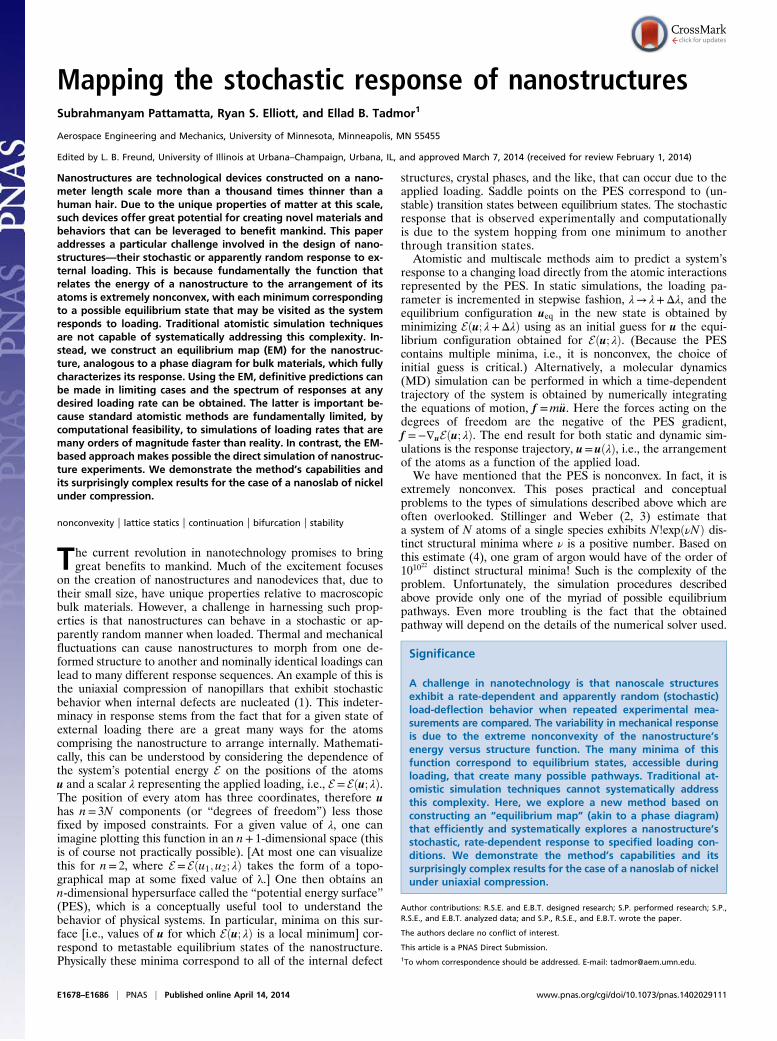
schematic one-dimensional model shown in Fig. 1. The surfacerepresents the dependence of an energy function E on a singledegree of freedom u and loading parameter !. A surface of thistype is typical of systems undergoing buckling, such as the classic

Fig. 1. Schematic illustrating the evolution of a PES as a function of a loadingparameter and the associated EM.

Pattamatta et al. PNAS | Published online April 14, 2014 | E1679

ENGINEE

RING

PNASPL

US

case of a thin-walled axially compressed cylindrical shell. Usingthe physics of such shells as a motivating example, we understandthe figure as follows. The shell exists in a stable cylindricalconfiguration at low values of axial compression (low values of !)and in a buckled configuration at high compression. The curvesin Fig. 1 (Insets) show the PES at different compressive loads.The transition from the single-well cylindrical configuration totwo symmetry-related variants of the buckled configuration isclear. The diagram at the bottom of the figure shows the EM forthe system. The solid lines correspond to stable (local energyminimizing) equilibrium configurations and the dashed lines tounstable (local maximum or saddle point) equilibrium config-urations. As the compressive load is continuously increased, thewell associated with the cylindrical configuration becomes moreshallow and eventually transforms into a maximum losing itsstability at high compression. At the point of change in topographyfrom a minimum to a maximum, the Hessian becomes singular ata bifurcation point. The two dashed golden-brown segments bi-furcating from the primary path represent the first generationpaths. Points along this path correspond to the maxima sepa-rating the cylindrical and buckled configurations and are thusunstable. These paths connect to the stable buckled configurationminima at turning points.Given the extreme nonconvexity of the PES, the construction

of the EM for realistic systems is a daunting task that is only nowbecoming possible due to recent developments in BFB algo-rithms for massively parallel supercomputers. In practice, an EMis generated by tracing a single solution curve and identifyingall bifurcation points, then returning to the bifurcation points,tracing out the connecting curves and their bifurcation points,and so on in a recursive fashion. This process is ideal for par-allelization because the calculation of each curve is independentof the others.There is a rich literature dealing with the characterization of

local bifurcations. For example, see refs. 6–15. There is alsoa mature literature on numerical branch-following (continua-tion) algorithms, including refs. 5, 16–19. These methodologieshave been applied in a variety of settings including problems incrystal and atomic-scale stability (20–25).The exploitation of symmetry in the construction of the EM is

often a critical step. In fact, the existence of bifurcation points isusually due to the presence of symmetry (as exemplified in Fig.1). Once the symmetry group of a PES function is identified, thetheory of equivariant systems (17, 26) can be used to reduce thedimension of the equilibrium equations and significantly improvethe computational efficiency of the branch-following procedure.

This reduction of dimension also regularizes the equilibriumequations near bifurcation points allowing for the accurate nu-merical determination of these points. Further, the use of equiv-ariant bifurcation theory (14, 17, 26–28) shows that once oneequilibrium path has been computed all symmetry-related pathsmay be constructed without further computation. These theo-retical and computational techniques must play a central role inany automated approach for the generation of the EM.

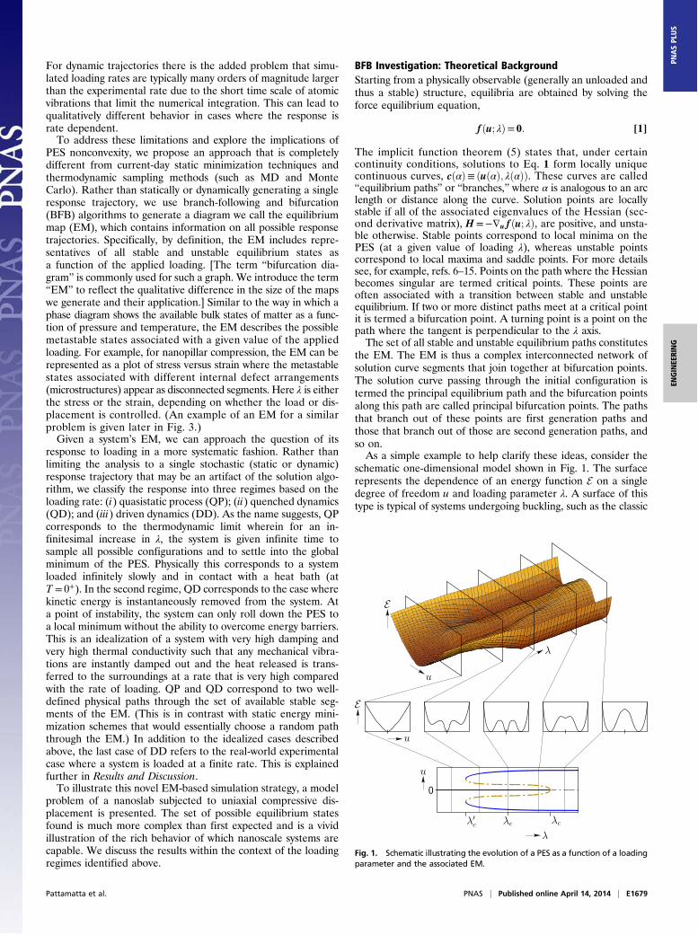
Compression of a Face-Centered Cubic Nanoslab of NickelAs an example of the EM-based simulation methodology, we focuson a simple atomistic application as a model problem. A face-centered cubic (fcc) nickel nanoslab of finite width and heightand infinite thickness in the out-of-plane direction is uniformlycompressed by a controlled displacement of its top and bottomsurfaces as shown in Fig. 2. [Note that the EM can be used forthe interpretation of both displacement and load control prob-lems. However, in this publication we restrict our discussion tothe displacement control case.] The nanoslab contains 104 un-constrained atoms (per unit depth) for a total of 312 degrees offreedom. For this problem, ! is the compressive displacement ofthe nanoslab and u is the column vector of nuclear coordinates.The atomic interactions are modeled by an embedded atommethod potential for nickel due to Angelo et al. (29) and Baskeset al. (30) modified to have smooth first and second derivatives.

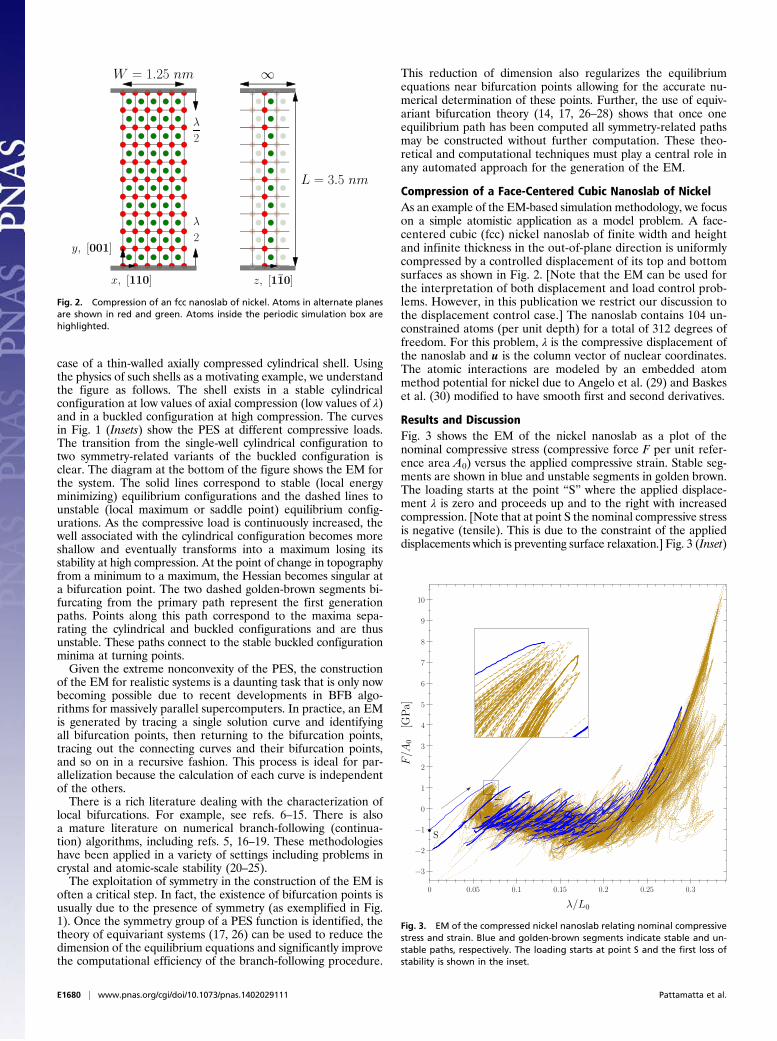
Results and DiscussionFig. 3 shows the EM of the nickel nanoslab as a plot of thenominal compressive stress (compressive force F per unit refer-ence area A0) versus the applied compressive strain. Stable seg-ments are shown in blue and unstable segments in golden brown.The loading starts at the point “S” where the applied displace-ment ! is zero and proceeds up and to the right with increasedcompression. [Note that at point S the nominal compressive stressis negative (tensile). This is due to the constraint of the applieddisplacements which is preventing surface relaxation.] Fig. 3 (Inset)

Fig. 2. Compression of an fcc nanoslab of nickel. Atoms in alternate planesare shown in red and green. Atoms inside the periodic simulation box arehighlighted.

Fig. 3. EM of the compressed nickel nanoslab relating nominal compressivestress and strain. Blue and golden-brown segments indicate stable and un-stable paths, respectively. The loading starts at point S and the first loss ofstability is shown in the inset.

E1680 | www.pnas.org/cgi/doi/10.1073/pnas.1402029111 Pattamatta et al.

shows in more detail the point of initial loss of stability on theprimary path. This EM contains 8,026 solution curves (after re-moving symmetry-related curves), of which 1,306 are stable witha total of 5.8 million distinct solution points. It was generated on256 processors of a parallel cluster over about 2 wk of wall timeand to our knowledge constitutes the largest BFB simulationperformed to date. With the data from the EM, we present se-lection rules of the stable paths representing the different loadingregimes discussed earlier.We first set out to identify the QP path where at each value of

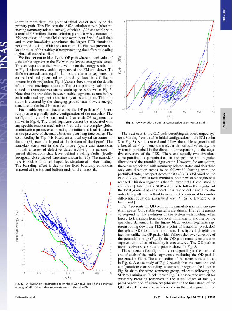
! the stable segment in the EM with the lowest energy is selected.This corresponds to the lower envelope on the energy–strain plotin Fig. 4 where only stable segments of the EM are shown. Todifferentiate adjacent equilibrium paths, alternate segments arecolored red and green and are joined by black lines if discon-tinuous in this projection. Fig. 4 (Insets) show some of the detailsof the lower envelope structure. The corresponding path repre-sented in (compressive) stress–strain space is shown in Fig. 5.Note that the transition between stable segments occurs beforeeach individual segment loses stability at its end point. The tran-sition is dictated by the changing ground state (lowest-energy)structure as the load is increased.Each stable segment traversed by the QP path in Fig. 5 cor-

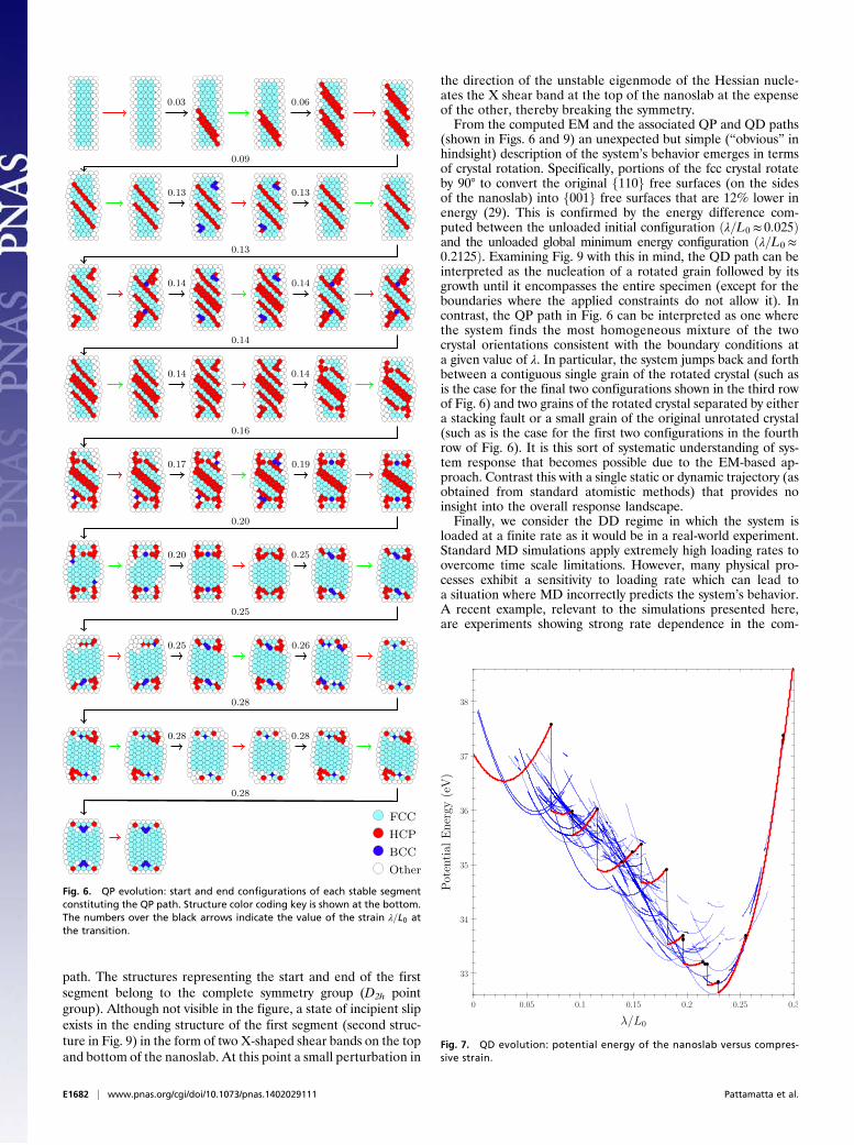
responds to a globally stable configuration of the nanoslab. Theconfigurations at the start and end of each QP segment areshown in Fig. 6. The black segments cannot be associated withany specific reaction mechanisms, but rather are complex globalminimization processes connecting the initial and final structuresin the presence of thermal vibrations over long time scales. Thecolor coding in Fig. 6 is based on a local crystal structure in-dicator (31) (see the legend at the bottom of the figure). Thenanoslab starts out in the fcc phase (cyan) and transitionsthrough a series of defective states involving the passage ofpartial dislocations that leave behind stacking faults (locallyhexagonal close-packed structures shown in red). The nanoslabreverts back to a barrel-shaped fcc structure at higher loading.The barreling effect is due to the fixed boundary conditionsimposed at the top and bottom ends of the nanoslab.

The next case is the QD path describing an overdamped sys-tem. Starting from a stable initial configuration in the EM (pointS in Fig. 3), we increase ! and follow the stable segment untila loss of stability is encountered. At this critical value, !cr, thesystem is perturbed in the direction corresponding to the nega-tive curvature of the PES. [There are actually two directionscorresponding to perturbations in the positive and negativedirections of the unstable eigenvector. However, for our system,these are associated with symmetry-related states and thereforeonly one direction needs to be followed.] Starting from theperturbed state, a steepest descent path (SDP) is followed on thePES, E!u; !cr", until a local minimum on a new stable segment isreached. This new segment is then followed until it loses stabilityand so on. [Note that the SDP is defined to follow the negative ofthe local gradient at each point. It is traced out using a fourth-order Runge–Kutta method to integrate the system of first-orderdifferential equations given by du=d#= f !u!#"; !cr", where !cr isheld fixed.]Fig. 7 presents the QD path of the nanoslab system in energy–

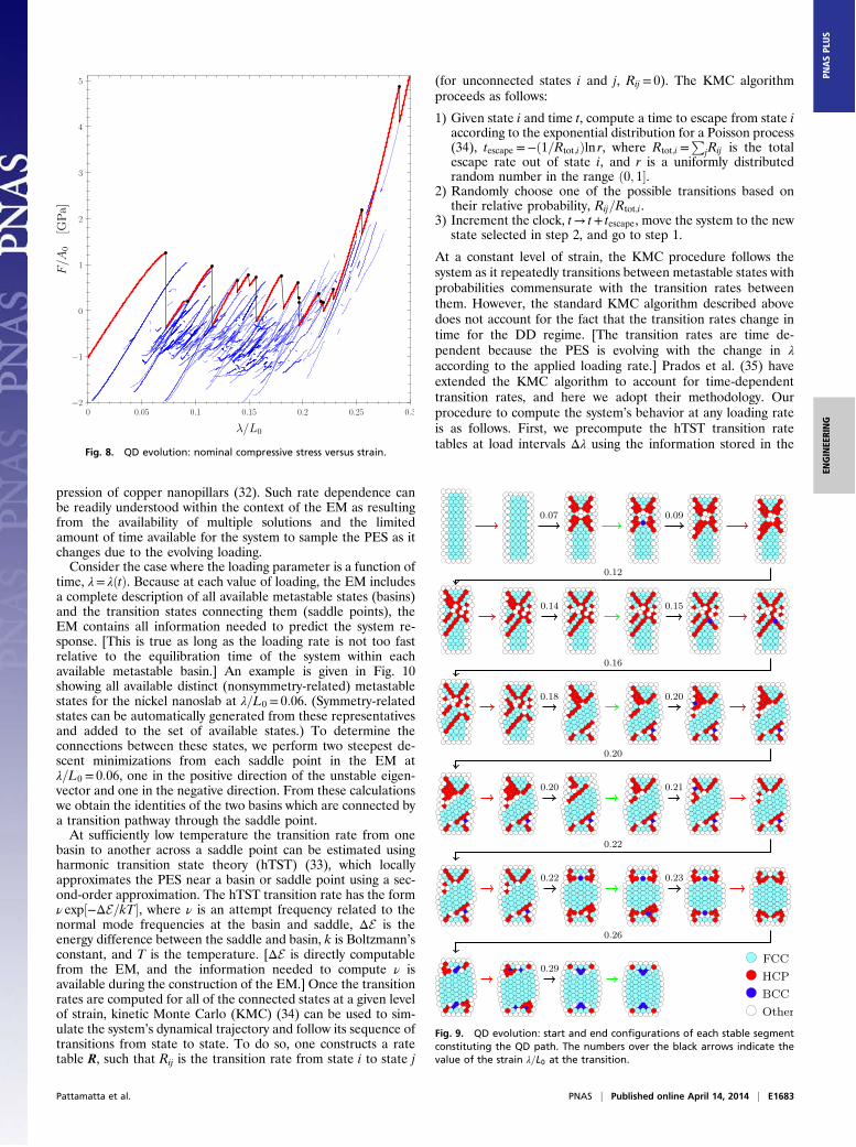
strain space. Only stable segments are shown. The red segmentscorrespond to the evolution of the system with loading whenforced to transition from one local minimum to another by thequenched dynamics. In the figure, black vertical segments rep-resent rolling down the PES at a point of instability (black dot)through an SDP to another minimum. This figure highlights thefact that unlike the QP path, which follows the lower envelope ofthe potential energy (Fig. 4), the QD path remains on a stablesegment until a loss of stability is encountered. The QD path in(compressive) stress–strain space is shown in Fig. 8.The sequence of configurations corresponding to the start and

end of each of the stable segments constituting the QD path ispresented in Fig. 9. The color coding of the atoms is the same asin Fig. 6. A close study of Fig. 9 reveals that the start and endconfigurations corresponding to each stable segment (red lines inFig. 8) share the same symmetry group, whereas following theSDP to a minimum (black lines in Fig. 8) is associated with eithersymmetry breaking (observed in the initial stages of the QDpath) or addition of symmetry (observed in the final stages of theQD path). This can be clearly observed in the first segment of the

Fig. 4. QP evolution constructed from the lower envelope of the potentialenergy of all of the stable segments constituting the EM.

Fig. 5. QP evolution: nominal compressive stress versus strain.

Pattamatta et al. PNAS | Published online April 14, 2014 | E1681

ENGINEE

RING

PNASPL

US

path. The structures representing the start and end of the firstsegment belong to the complete symmetry group (D2h pointgroup). Although not visible in the figure, a state of incipient slipexists in the ending structure of the first segment (second struc-ture in Fig. 9) in the form of two X-shaped shear bands on the topand bottom of the nanoslab. At this point a small perturbation in

the direction of the unstable eigenmode of the Hessian nucle-ates the X shear band at the top of the nanoslab at the expenseof the other, thereby breaking the symmetry.From the computed EM and the associated QP and QD paths

(shown in Figs. 6 and 9) an unexpected but simple (“obvious” inhindsight) description of the system’s behavior emerges in termsof crystal rotation. Specifically, portions of the fcc crystal rotateby 90° to convert the original f110g free surfaces (on the sidesof the nanoslab) into f001g free surfaces that are 12% lower inenergy (29). This is confirmed by the energy difference com-puted between the unloaded initial configuration !!=L0 $ 0:025"and the unloaded global minimum energy configuration !!=L0 $0:2125". Examining Fig. 9 with this in mind, the QD path can beinterpreted as the nucleation of a rotated grain followed by itsgrowth until it encompasses the entire specimen (except for theboundaries where the applied constraints do not allow it). Incontrast, the QP path in Fig. 6 can be interpreted as one wherethe system finds the most homogeneous mixture of the twocrystal orientations consistent with the boundary conditions ata given value of !. In particular, the system jumps back and forthbetween a contiguous single grain of the rotated crystal (such asis the case for the final two configurations shown in the third rowof Fig. 6) and two grains of the rotated crystal separated by eithera stacking fault or a small grain of the original unrotated crystal(such as is the case for the first two configurations in the fourthrow of Fig. 6). It is this sort of systematic understanding of sys-tem response that becomes possible due to the EM-based ap-proach. Contrast this with a single static or dynamic trajectory (asobtained from standard atomistic methods) that provides noinsight into the overall response landscape.Finally, we consider the DD regime in which the system is

loaded at a finite rate as it would be in a real-world experiment.Standard MD simulations apply extremely high loading rates toovercome time scale limitations. However, many physical pro-cesses exhibit a sensitivity to loading rate which can lead toa situation where MD incorrectly predicts the system’s behavior.A recent example, relevant to the simulations presented here,are experiments showing strong rate dependence in the com-

Fig. 6. QP evolution: start and end configurations of each stable segmentconstituting the QP path. Structure color coding key is shown at the bottom.The numbers over the black arrows indicate the value of the strain !=L0 atthe transition.

Fig. 7. QD evolution: potential energy of the nanoslab versus compres-sive strain.

E1682 | www.pnas.org/cgi/doi/10.1073/pnas.1402029111 Pattamatta et al.

pression of copper nanopillars (32). Such rate dependence canbe readily understood within the context of the EM as resultingfrom the availability of multiple solutions and the limitedamount of time available for the system to sample the PES as itchanges due to the evolving loading.Consider the case where the loading parameter is a function of

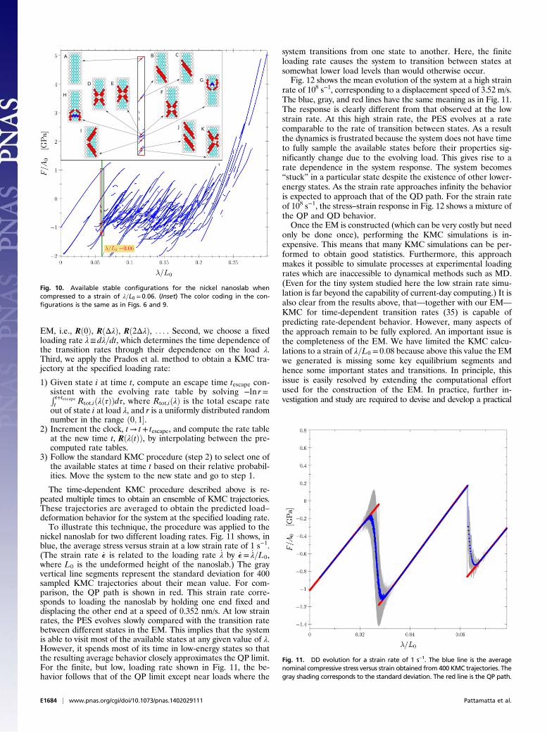
time, != !!t". Because at each value of loading, the EM includesa complete description of all available metastable states (basins)and the transition states connecting them (saddle points), theEM contains all information needed to predict the system re-sponse. [This is true as long as the loading rate is not too fastrelative to the equilibration time of the system within eachavailable metastable basin.] An example is given in Fig. 10showing all available distinct (nonsymmetry-related) metastablestates for the nickel nanoslab at !=L0 = 0:06. (Symmetry-relatedstates can be automatically generated from these representativesand added to the set of available states.) To determine theconnections between these states, we perform two steepest de-scent minimizations from each saddle point in the EM at!=L0 = 0:06, one in the positive direction of the unstable eigen-vector and one in the negative direction. From these calculationswe obtain the identities of the two basins which are connected bya transition pathway through the saddle point.At sufficiently low temperature the transition rate from one

basin to another across a saddle point can be estimated usingharmonic transition state theory (hTST) (33), which locallyapproximates the PES near a basin or saddle point using a sec-ond-order approximation. The hTST transition rate has the form" exp#!ΔE=kT$, where " is an attempt frequency related to thenormal mode frequencies at the basin and saddle, ΔE is theenergy difference between the saddle and basin, k is Boltzmann’sconstant, and T is the temperature. [ΔE is directly computablefrom the EM, and the information needed to compute " isavailable during the construction of the EM.] Once the transitionrates are computed for all of the connected states at a given levelof strain, kinetic Monte Carlo (KMC) (34) can be used to sim-ulate the system’s dynamical trajectory and follow its sequence oftransitions from state to state. To do so, one constructs a ratetable R, such that Rij is the transition rate from state i to state j

(for unconnected states i and j, Rij = 0). The KMC algorithmproceeds as follows:

1) Given state i and time t, compute a time to escape from state iaccording to the exponential distribution for a Poisson process(34), tescape =!!1=Rtot;i"ln r, where Rtot;i =

PjRij is the total

escape rate out of state i, and r is a uniformly distributedrandom number in the range !0; 1$.

2) Randomly choose one of the possible transitions based ontheir relative probability, Rij=Rtot;i.

3) Increment the clock, t! t+ tescape, move the system to the newstate selected in step 2, and go to step 1.

At a constant level of strain, the KMC procedure follows thesystem as it repeatedly transitions between metastable states withprobabilities commensurate with the transition rates betweenthem. However, the standard KMC algorithm described abovedoes not account for the fact that the transition rates change intime for the DD regime. [The transition rates are time de-pendent because the PES is evolving with the change in !according to the applied loading rate.] Prados et al. (35) haveextended the KMC algorithm to account for time-dependenttransition rates, and here we adopt their methodology. Ourprocedure to compute the system’s behavior at any loading rateis as follows. First, we precompute the hTST transition ratetables at load intervals Δ! using the information stored in the

Fig. 8. QD evolution: nominal compressive stress versus strain.

Fig. 9. QD evolution: start and end configurations of each stable segmentconstituting the QD path. The numbers over the black arrows indicate thevalue of the strain !=L0 at the transition.

Pattamatta et al. PNAS | Published online April 14, 2014 | E1683

ENGINEE

RING

PNASPL

US

EM, i.e., R!0", R!Δ!", R!2Δ!", . . . . Second, we choose a fixedloading rate _!# d!=dt, which determines the time dependence ofthe transition rates through their dependence on the load !.Third, we apply the Prados et al. method to obtain a KMC tra-jectory at the specified loading rate:

1) Given state i at time t, compute an escape time tescape con-sistent with the evolving rate table by solving !ln r=R t+tescapet Rtot;i!!!$""d$, where Rtot;i!!" is the total escape rateout of state i at load !, and r is a uniformly distributed randomnumber in the range !0; 1$.

2) Increment the clock, t! t+ tescape, and compute the rate tableat the new time t, R!!!t"", by interpolating between the pre-computed rate tables.

3) Follow the standard KMC procedure (step 2) to select one ofthe available states at time t based on their relative probabil-ities. Move the system to the new state and go to step 1.

The time-dependent KMC procedure described above is re-peated multiple times to obtain an ensemble of KMC trajectories.These trajectories are averaged to obtain the predicted load–deformation behavior for the system at the specified loading rate.To illustrate this technique, the procedure was applied to the

nickel nanoslab for two different loading rates. Fig. 11 shows, inblue, the average stress versus strain at a low strain rate of 1 s!1.(The strain rate _e is related to the loading rate _! by _e= _!=L0,where L0 is the undeformed height of the nanoslab.) The grayvertical line segments represent the standard deviation for 400sampled KMC trajectories about their mean value. For com-parison, the QP path is shown in red. This strain rate corre-sponds to loading the nanoslab by holding one end fixed anddisplacing the other end at a speed of 0.352 nm/s. At low strainrates, the PES evolves slowly compared with the transition ratebetween different states in the EM. This implies that the systemis able to visit most of the available states at any given value of !.However, it spends most of its time in low-energy states so thatthe resulting average behavior closely approximates the QP limit.For the finite, but low, loading rate shown in Fig. 11, the be-havior follows that of the QP limit except near loads where the

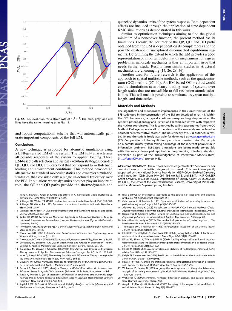
system transitions from one state to another. Here, the finiteloading rate causes the system to transition between states atsomewhat lower load levels than would otherwise occur.Fig. 12 shows the mean evolution of the system at a high strain

rate of 108 s!1, corresponding to a displacement speed of 3.52 m/s.The blue, gray, and red lines have the same meaning as in Fig. 11.The response is clearly different from that observed at the lowstrain rate. At this high strain rate, the PES evolves at a ratecomparable to the rate of transition between states. As a resultthe dynamics is frustrated because the system does not have timeto fully sample the available states before their properties sig-nificantly change due to the evolving load. This gives rise to arate dependence in the system response. The system becomes“stuck” in a particular state despite the existence of other lower-energy states. As the strain rate approaches infinity the behavioris expected to approach that of the QD path. For the strain rateof 108 s!1, the stress–strain response in Fig. 12 shows a mixture ofthe QP and QD behavior.Once the EM is constructed (which can be very costly but need

only be done once), performing the KMC simulations is in-expensive. This means that many KMC simulations can be per-formed to obtain good statistics. Furthermore, this approachmakes it possible to simulate processes at experimental loadingrates which are inaccessible to dynamical methods such as MD.(Even for the tiny system studied here the low strain rate simu-lation is far beyond the capability of current-day computing.) It isalso clear from the results above, that—together with our EM—KMC for time-dependent transition rates (35) is capable ofpredicting rate-dependent behavior. However, many aspects ofthe approach remain to be fully explored. An important issue isthe completeness of the EM. We have limited the KMC calcu-lations to a strain of !=L0 = 0:08 because above this value the EMwe generated is missing some key equilibrium segments andhence some important states and transitions. In principle, thisissue is easily resolved by extending the computational effortused for the construction of the EM. In practice, further in-vestigation and study are required to devise and develop a practical

Fig. 10. Available stable configurations for the nickel nanoslab whencompressed to a strain of !=L0 = 0:06. (Inset) The color coding in the con-figurations is the same as in Figs. 6 and 9.

Fig. 11. DD evolution for a strain rate of 1 s!1. The blue line is the averagenominal compressive stress versus strain obtained from 400 KMC trajectories. Thegray shading corresponds to the standard deviation. The red line is the QP path.

E1684 | www.pnas.org/cgi/doi/10.1073/pnas.1402029111 Pattamatta et al.

and robust computational scheme that will automatically gen-erate important components of the full EM.

ConclusionsA new technique is proposed for atomistic simulations usinga BFB-generated EM of the system. The EM fully characterizesall possible responses of the system to applied loading. ThreeEM-based path selection and system evolution strategies, denotedQP, QD, and DD, are described that correspond to well-definedloading and environment conditions. This method provides analternative to standard molecular statics and dynamics simulationstrategies that consider only a single ill-defined trajectory overthe PES. In situations where dynamics does not play an importantrole, the QP and QD paths provide the thermodynamic and

quenched dynamics limits of the system response. Rate-dependenteffects are included through the application of time-dependentKMC simulations as demonstrated in this work.Similar to optimization techniques aiming to find the global

minimum of a nonconvex function, the present method has itslimitations. Clearly, the accuracy of the QP, QD, and DD pathsobtained from the EM is dependent on its completeness and thepossible existence of unexplored disconnected equilibrium seg-ments. Determining the extent to which the EM provides a goodrepresentation of important deformation mechanisms for a givenproblem in nanoscale mechanics is thus an important issue thatneeds further study. Results from similar studies in structuralmechanics are encouraging (14, 26, 28, 36).Another area for future research is the application of this

approach to spatial multiscale methods, such as the quasicontin-uum (QC) method (37–40). An EM-based QC method wouldenable simulations at arbitrary loading rates of systems overlength scales that are unavailable to full-resolution atomic calcu-lations. This will make it possible to simultaneously span multiplelength- and time-scales.

Materials and MethodsThe algorithms and pseudocodes implemented in the current version of theBFB code used in the construction of the EM are described in ref. 41. Withinthe BFB framework, a typical continuation–quenching step requires thesystem’s potential energy and its first and second derivatives with respect tothe nuclear coordinates. This is computed by calling subroutines from the QCMethod Package, wherein all of the atoms in the nanoslab are declared asnonlocal “representative atoms.” The basic theory of QC is outlined in refs.39, 40 and the code is freely available for download at www.qcmethod.org(42). Computation of the equilibrium paths is automated using Perl scriptson a parallel cluster system taking advantage of the inherent parallelism inbifurcation problems. EM-based simulations are being made compatiblewith the newly developed application programming interface standarddeveloped as part of the Knowledgebase of Interatomic Models (KIM)(http://openKIM.org) project (43).

ACKNOWLEDGMENTS. The authors acknowledge Tsvetanka Sendova for hercontributions to the initial stages of this work. This work was partlysupported by the National Science Foundation (NSF) Cyber-Enabled Discoveryand Innovation (CDI) Grant Phy-0941493 (to R.S.E. and E.B.T.), NSF CAREERGrant CMMI-0746628 (to R.S.E.), Department of Energy Grant DE-SC0002085(to E.B.T.), the Office of the Vice President for Research, University of Minnesota,and the Minnesota Supercomputing Institute.

1. Kunz A, Pathak S, Greer JR (2011) Size effects in AI nanopillars: Single crystalline vs.bicrystalline. Acta Mater 59(11):4416–4424.

2. Stillinger FH, Weber TA (1982) Hidden structure in liquids. Phys Rev A 25(2):978–989.3. Stillinger FH, Weber TA (1983) Dynamics of structural transitions in liquids. Phys Rev A

28(10):2408–2416.4. Stillinger FH, Weber TA (1984) Packing structures and transitions in liquids and solids.

Science 225(4666):983–989.5. Keller HB (1987) Lectures on Numerical Methods in Bifurcation Problems, Tata In-

stitute of Fundamental Research Lectures on Mathematics and Physics: Mathematics(Springer, Berlin).

6. Thompson JMT, Hunt GW (1973) A General Theory of Elastic Stability (John Wiley andSons, London), 1st Ed.

7. Thompson JMT (1982) Instabilities and Catastrophes in Science and Engineering (JohnWiley and Sons, London), 1st Ed.

8. Thompson JMT, Hunt GW (1984) Elastic Instability Phenomena (Wiley, New York), 1st Ed.9. Golubitsky M, Schaeffer DG (1984) Singularities and Groups in Bifurcation Theory.

Volume 1, Applied Mathematical Sciences (Springer, Berlin), 1st Ed, Vol. 51.10. Golubitsky M, Stewart I, Schaeffer DG (1988) Singularities and Groups in Bifurcation

Theory. Volume 2, Applied Mathematical Sciences (Springer, Berlin), 1st Ed., Vol. 69.11. Iooss G, Joseph DD (1997) Elementary Stability and Bifurcation Theory, Undergradu-

ate Texts in Mathematics (Springer, New York), 2nd Ed.12. Govaerts WJ (2000) Numerical Methods for Bifurcations of Dynamical Equilibria (So-

ciety for Industrial and Applied Mathematics, Philadelphia).13. Buffoni B, Toland J (2003) Analytic Theory of Global Bifurcation: An Introduction,

Princeton Series in Applied Mathematics (Princeton Univ Press, Princeton), 1st Ed.14. Ikeda K, Murota K (2010) Imperfect Bifurcation in Structures and Materials: Engi-

neering Use of Group-Theoretic Bifurcation Theory, Applied Mathematical Sciences(Springer, New York), 2nd Ed, Vol 149.

15. Seydel R (2010) Practical Bifurcation and Stability Analysis, Interdisciplinary AppliedMathematics (Springer, New York), 3rd Ed, Vol 5.

16. Riks E (1979) An incremental approach to the solution of snapping and bucklingproblems. Int J Solids Struct 15(7):529–551.

17. Gatermann K, Hohmann A (1991) Symbolic exploitation of symmetry in numericalpathfollowing. Imp Comput Sci Eng 3(4):330–365.

18. Allgower EL, Georg K (2003) Introduction to Numerical Continuation Methods, Classics.AppliedMathematics (Society for Industrial and AppliedMathematics, Philadelphia), Vol 45.

19. Dankowicz H, Schilder F (2013) Recipes for Continuation, Computational Science andEngineering (Society for Industrial and Applied Mathematics, Philadelphia).

20. Macmillan NH, Kelly A (1972) The mechanical properties of perfect crystals. I. Theideal strength. Proc R Soc Lond A 330(1582):291–308.

21. Thompson JMT, Shorrock PA (1975) Bifurcational instability of an atomic lattice.J Mech Phys Solids 23(1):21–37.

22. Elliott RS, Triantafyllidis N, Shaw JA (2006) Stability of crystalline solids—I: Continuumand atomic lattice considerations. J Mech Phys Solids 54(1):161–192.

23. Elliott RS, Shaw JA, Triantafyllidis N (2006) Stability of crystalline solids—II: Applica-tion to temperature-induced martensitic phase transformations in a bi-atomic crystal.J Mech Phys Solids 54(1):193–232.

24. Elliott RS (2007) Multiscale bifurcation and stability of multilattices. J Comput AidedMater Des 14(Suppl 1):143–157.

25. Delph TJ, Zimmerman JA (2010) Prediction of instabilities at the atomic scale. ModelSimul Mater Sci Eng 18(4):045008.

26. Healey TJ (1988) A group-theoretic approach to computational bifurcation problemswith symmetry. Comput Methods Appl Mech Eng 67(3):257–295.

27. Wohlever JC, Healey TJ (1995) A group theoretic approach to the global bifurcationanalysis of an axially compressed cylindrical shell. Comput Methods Appl Mech Eng122(3-4):315–349.

28. Wohlever JC (1996) Symmetry, nonlinear bifurcation analysis, and parallel computa-tion. (Cornell University, Ithaca, NY).

29. Angelo JE, Moody NR, Baskes MI (1995) Trapping of hydrogen to lattice-defects innickel. Model Simul Mater Sci Eng 3(3):289–307.

Fig. 12. DD evolution for a strain rate of 108 s!1. The blue, gray, and redlines have the same meaning as in Fig. 11.

Pattamatta et al. PNAS | Published online April 14, 2014 | E1685

ENGINEE

RING

PNASPL

US

30. Baskes MI, Sha XW, Angelo JE, Moody NR (1997) Trapping of hydrogen to latticedefects in nickel. Model Simul Mater Sci Eng 5(6):651–652.

31. Stukowski A (2010) Visualization and analysis of atomistic simulation data with ovito-the open visualization tool. Model Simul Mater Sci Eng 18(1):015012.

32. Jennings AT, Li J, Greer JR (2011) Emergence of strain-rate sensitivity in Cu nano-pillars: Transition from dislocation multiplication to dislocation nucleation. ActaMater 59(14):5627–5637.

33. Vineyard GH (1957) Frequency factors and isotope effects in solid state rate processes.J Phys Chem Solids 3(1-2):121–127.

34. Voter AF (2005) Radiation Effects in Solids, eds Sickafus KE, Kotomin EA (Springer,NATO Publishing Unit, Dordrecht, The Netherlands).

35. Prados A, Brey JJ, Sánchez-Rey B (1997) A dynamical Monte Carlo algorithm formaster equations with time-dependent transition rates. J Stat Phys 89(3-4):709–734.

36. Budiansky B (1974) Advances in Applied Mechanics, ed Yih CS (Academic, New York),Vol 14, pp 1–65.

37. Tadmor EB, Ortiz M, Phillips R (1996) Quasicontinuum analysis of defects in solids. PhilMag A73(6):1529–1563.

38. Shenoy VB, et al. (1999) An adaptive methodology for atomic scale mechanics: Thequasicontinuum method. J Mech Phys Solids 47(3):611–642.

39. Miller RE, Tadmor EB (2002) The quasicontinuummethod: Overview, applications andcurrent directions. J Comput Aided Mater Des 9(3):203–239.

40. Tadmor EB, Miller RE (2011) Modeling Materials: Continuum, Atomistic and Multi-scale Techniques (Cambridge Univ Press, Cambridge, UK).

41. Jusuf V (2010) Algorithms for branch-following and critical point identification in thepresence of symmetry. Master’s thesis (University of Minnesota, Minneapolis).

42. Tadmor EB, Miller RE (2003) The Quasicontinuum Method Website. Available atwww.qcmethod.org. Last accessed February 1, 2014.

43. Tadmor EB, Elliott RS, Sethna JP, Miller RE, Becker CA (2011) The potential of atomisticsimulations and the Knowledgebase of Interatomic Models (KIM). JOM 63(7):17.

E1686 | www.pnas.org/cgi/doi/10.1073/pnas.1402029111 Pattamatta et al.