1
Analysis of flow and wave motion in an electromagnetic streamer at the FloWave tank A. Tcheheumeni, A. Ziolkowski and D. Wright The University of Edinburgh [email protected] Abstract I The performance of the towed streamer EM system is dependent on noise levels in the acquired data. I It is important to understand the nature and the relative contribution of different sources of noise in order to reduce the noise level in the towed EM system. I To achieve this goal, we carried out various tests on a prototype EM streamer in the controlled environment of the new FloWave tank. The noise level was found to increase with increasing flow velocity. The motion of the prototype EM streamer in response to a parallel constant current (0.5m/s) and a 0.1 m amplitude wave motion of 0.29Hz was found to generate significant noise. The electric field was found to be very well correlated with the motion of the cable. 1. Introduction I Towed streamer EM receivers and an electric current bi-pole source towed at 4 - 5 knots are used for efficient acquisition of controlled source electromagnetic (CSEM) data as shown in Figure 1. I Towed-streamer receivers enable faster and more efficient data acquisition compared to traditional node receivers. Figure 1:The towed streamer EM from PGS website. Although the increase in efficiency is obvious, the system can be affected by noise from various sources as summarised in Figure 2. Problem Figure 2: Sources of noise present in the towed EM system. The main question is, can we identify and quantify the contribution of each of these sources of noise? To address this question: We built a 16m long 13 channel prototype EM streamer. We investigated the effect (on noise levels) of increasing water flow rate and wave motion at different frequencies (0.29Hz and 0.45Hz) and amplitudes (0.1m and 0.15m) around a prototype EM streamer. We recorded motion capture data of the streamer moving in order to analyse the relation between the electric field and the cable motion. Aim 2. Experimental setup (a) Location I Located at the University of Edinburgh, United Kingdom. I Circular tank with a diameter of 25m and water depth of 3m as shown in Figure 3. I The tank can generate current velocity of up to 1.5m/s and a wave amplitude and frequency of up to 0.15m and 0.45Hz respectively. Figure 3: FloWave tank. Sampling frequency = 50 Hz, active streamer length-16m, 13 electric field channels with AgAgCl electrodes in the streamer and 2 fixed channels with the telluric cable running out the water as depicted in Figure 4, 4 motion capture cameras and 21 reflective stickers spread in the middle section of the streamer (4m), see Figure 4. 5 electrode wiring configuration were used during the test. Only results from the configuration shown in Figure 5 are presented here. Test 1: The effect of flow. Data are acquired for flow rates of 0, 0.5, 1 and 1.5m/s respectively. Test 2: The effect of wave motion. Data were ac- quired with a wave frequency and amplitude 0.29Hz and 0.1m respectively and a constant flow of 0.5m/s. Aquisition parameters (b) Prototype EM streamer layout in the tank. 30 m 3 m Data Acquisition device Gantry Computer 1 m Motion capture cameras Prototype EM streamer Fixed electrodes Water surface Fixed electrodes cable return to DAQ Tank floor Reflective stickers (21) Electrodes (AgAgCl types) Y Z Not to scale X Wave / flow direction Figure 4: Layout of the streamer, the fixed electrodes and motion capture cameras. The rectangular dash box is the 4m section of the cable where the reflective stickers were attached. (Not to scale) (c) Electrode layout The electrode layout is illustrated in Figure 5. 1 2 4 3 5 6 8 7 9 1 1 1 0 1 3 1 2 1 4 1 8 1 6 1 7 2 0 1 9 2 2 2 1 2 4 2 3 1 5 2 m 2 m 2 m 1 m 0.75 m 0.5 m 0.25 m 0.75 m 2 m 2 m 2 m 1 m 0.5 m 0.25 m 0.5 m 0.5 m Channels outside the streamer ch1 Ch2 (0.25 m) Ch4 (1 m) Ch3 (0.5 m) Ch5 (2 m) Ch6 (2 m) Ch7 (4 m) Ch8 (4 m) Ch9 (4 m) Ch10 (4 m) Ch11 (8 m) Ch12 (8 m) Ch13 (8 m) Ch14 (8 m) Ch15 (8 m) Figure 5: Layout of the E-field data. channel 14 and 15 are fixed channels. 3. Results (a) Effect of flow The effect of flow was investigated by calculating the average RMS of data recorded when flow rate is 0, 0.5, 1 and 1.5m/s respectively. The results is shown in Figure 6. ch1 ch2 ch3 ch4 ch5 ch6 ch7 ch8 ch9 ch10 ch11 ch12 ch13 0 0.2 0.4 0.6 0.8 1 1.2 1.4 1.6 1.8 2 x 10 -5 Channel number Average root-mean-square amplitude (V) Current velocity = 0 m/s Current velocity = 0.5 m/s Current velocity = 1 m/s Current velocity = 1.5 m/s ch1 ch2 ch3 ch4 ch5 ch6 ch7 ch8 ch9 ch10 ch11 ch12 ch13 0 1 2 3 4 5 6 7 8 x 10 -5 Channel number Average root-mean-square amplitude (V/m) Figure 6: The average RMS noise amplitude in the time domain in the case of still water and constant flow at rates up to 1.5m/s. The small window on the top right, represents the same data but normalised by the channel length. Therefore, it is in volts per metre (V/m). (b) Effect of wave motion 0 10 20 30 40 50 60 70 -0.1 -0.05 0 0.05 0.1 Amplitude (m) (a) Time series Input sine wave (0.29Hz) 0 10 20 30 40 50 60 70 -0.04 -0.02 0 0.02 0.04 0.06 X-displacement (m) 0 10 20 30 40 50 60 70 -0.06 -0.04 -0.02 0 0.02 0.04 0.06 Y-displacement (m) 0 10 20 30 40 50 60 70 -0.06 -0.04 -0.02 0 0.02 0.04 0.06 Z-diplacement (m) Time (s) 0 0.1 0.2 0.3 0.4 0.5 0.6 0.7 0.8 0.9 1 0 0.002 0.004 0.006 0.008 0.01 0.012 0.014 0.016 0.018 0.02 Frequency (Hz) Magnitude (b) Amplitude spectrum Input sine wave at 0.29 Hz X - amplitude spectrum Y - amplitude spectrum Z - amplitude spectrum Harmonics Figure 7: The X-, Y- and Z- displacement and resulting amplitude spectrum measured at the centre of the streamer in response to a 0.1m amplitude wave of frequency 0.29Hz flowing at 0.5m/s parallel to the streamer. (c) Measured electric field - Time and spectrum analysis Figure 8 shows electric fields measured from chan- nel 7 (4m electrode separation), channel 12 (8m separation) and channel 14 (fixed electrodes). 0 10 20 30 40 50 60 70 -0.1 -0.05 0 0.05 0.1 Amplitude (m) (a) Time series Input sine wave at 0.29 Hz 0 10 20 30 40 50 60 70 -1 -0.5 0 0.5 1 x 10 -5 E-field (V/m) channel 7 0 10 20 30 40 50 60 70 -1 -0.5 0 0.5 1 x 10 -5 E-field (V/m) channel 12 0 10 20 30 40 50 60 70 -1 -0.5 0 0.5 1 x 10 -5 E-field (V/m) Time (s) channel 14 0 0.1 0.2 0.3 0.4 0.5 0.6 0.7 0.8 0.9 1 0 0.2 0.4 0.6 0.8 1 1.2 1.4 1.6 1.8 2 x 10 -6 Frequency (Hz) Magnitude relative to 1V/m (b) Amplitude spectrum Input sine wave at 0.29 Hz Channel 7 Channel 12 Channel 14 Harmonics Figure 8: Data from channel 7 , channel 12 and channel 14. Data were recorded at the same time with the data shown in Figure 7. (d) Coherence analysis The magnitude squared coherence is a signal processing tool that provides a measure of how well two time series are correlated as a function of frequency. It varies between 0 and 1, where 0 means complety uncorrelated and 1 means perfectly correlated. 10 -1 10 0 10 1 0 0.1 0.2 0.3 0.4 0.5 0.6 0.7 0.8 0.9 1 Frequency (Hz) Magnitude squared coherence channel 7 and Z-displacement channel 12 and Z-displacement channel 14 and Z-displacement Channels inside the streamer Channel outside the streamer 0.3Hz Figure 9: Electric field and displacement in Z-direction coherence vs. frequency. The two signals in each coherence calculation are indicated in the legend. 4. Preliminary interpretation and conclusions I The RMS noise increases by approximately 40 % as flow is increased from 0 to 1.5m/s. However, most of this increase (36%) occurs between there being no flow and flow of 0.5m/s (Figure 6). I This indicates that the increase of flow rate increases the noise level in the towed EM streamer. Extrapolating these results to a flow rate of 2.5m/s at which towed streamer are acquired suggest an increase in the noise level of 45 % above the static noise level. I Channels inside the streamer are sensitive to wave motion. Fixed electrodes with the signal cable out of the water are not sensitive to wave motion (Figure 7, 8). I There is a strong correlation between channels inside the streamer and wave motion. In contrast the correlation is very low (0.12) between the channel fixed outside the streamer and the wave motion (Figure 9). I These results suggest that the motion of the streamer due to the wave motion is the major source of noise. I Future work will focus on relating the motion of the cable to the measured electric field. 5. Acknowledgements Axel Thanks Petroleum Geo-Services (PGS) for funding his research. Email: [email protected] Linkedin:https://uk.linkedin.com/in/tcheheumeni Address: Earth and Planetary Science, Grant Institute, EH9 3FE

Marelec2015.Tex

Embed Size (px)

DESCRIPTION

Analysis of flow and wave motion in an electromagnetic streamer at the FloWave tank

Citation preview

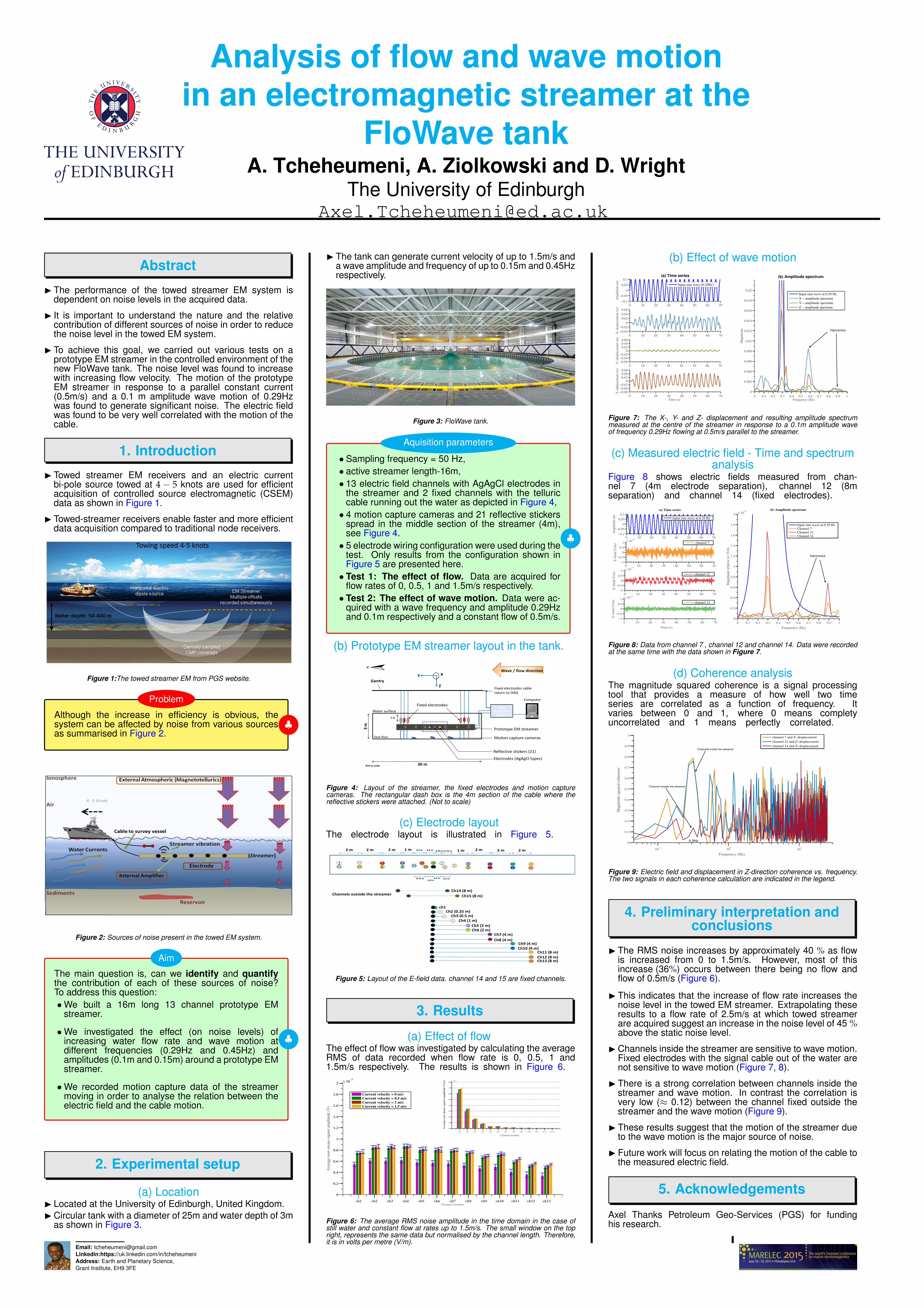
Analysis of flow and wave motionin an electromagnetic streamer at the

FloWave tankA. Tcheheumeni, A. Ziolkowski and D. Wright

The University of [email protected]

Abstract

I The performance of the towed streamer EM system isdependent on noise levels in the acquired data.

I It is important to understand the nature and the relativecontribution of different sources of noise in order to reducethe noise level in the towed EM system.

I To achieve this goal, we carried out various tests on aprototype EM streamer in the controlled environment of thenew FloWave tank. The noise level was found to increasewith increasing flow velocity. The motion of the prototypeEM streamer in response to a parallel constant current(0.5m/s) and a 0.1 m amplitude wave motion of 0.29Hzwas found to generate significant noise. The electric fieldwas found to be very well correlated with the motion of thecable.

1. Introduction

I Towed streamer EM receivers and an electric currentbi-pole source towed at 4− 5 knots are used for efficientacquisition of controlled source electromagnetic (CSEM)data as shown in Figure 1.

I Towed-streamer receivers enable faster and more efficientdata acquisition compared to traditional node receivers.

Figure 1:The towed streamer EM from PGS website.

Although the increase in efficiency is obvious, thesystem can be affected by noise from various sourcesas summarised in Figure 2.

Problem

Figure 2: Sources of noise present in the towed EM system.

The main question is, can we identify and quantifythe contribution of each of these sources of noise?To address this question:•We built a 16m long 13 channel prototype EM

streamer.

•We investigated the effect (on noise levels) ofincreasing water flow rate and wave motion atdifferent frequencies (0.29Hz and 0.45Hz) andamplitudes (0.1m and 0.15m) around a prototype EMstreamer.

•We recorded motion capture data of the streamermoving in order to analyse the relation between theelectric field and the cable motion.

Aim

2. Experimental setup

(a) LocationI Located at the University of Edinburgh, United Kingdom.I Circular tank with a diameter of 25m and water depth of 3m

as shown in Figure 3.

I The tank can generate current velocity of up to 1.5m/s anda wave amplitude and frequency of up to 0.15m and 0.45Hzrespectively.

Figure 3: FloWave tank.

• Sampling frequency = 50 Hz,• active streamer length-16m,• 13 electric field channels with AgAgCl electrodes in

the streamer and 2 fixed channels with the telluriccable running out the water as depicted in Figure 4,• 4 motion capture cameras and 21 reflective stickers

spread in the middle section of the streamer (4m),see Figure 4.• 5 electrode wiring configuration were used during the

test. Only results from the configuration shown inFigure 5 are presented here.• Test 1: The effect of flow. Data are acquired for

flow rates of 0, 0.5, 1 and 1.5m/s respectively.• Test 2: The effect of wave motion. Data were ac-

quired with a wave frequency and amplitude 0.29Hzand 0.1m respectively and a constant flow of 0.5m/s.

Aquisition parameters

(b) Prototype EM streamer layout in the tank.

30 m

3 m

Data Acquisition

device

Gantry

Computer

1 m

Motion capture cameras

Prototype EM streamer

Fixed electrodes

Water surface

Fixed electrodes cable return to DAQ

Tank floor

Reflective stickers (21)

Electrodes (AgAgCl types)

Y

Z

Not to scale

XWave / flow direction

Figure 4: Layout of the streamer, the fixed electrodes and motion capturecameras. The rectangular dash box is the 4m section of the cable where thereflective stickers were attached. (Not to scale)

(c) Electrode layoutThe electrode layout is illustrated in Figure 5.

12 4

3 56 8

79 1

1

1

013

12

14

18

16

17

20

19

22

21

24

23

15

2 m 2 m 2 m 1 m

0.75 m

0.5 m 0.25 m 0.75 m 2 m 2 m 2 m1 m0.5 m

0.25 m0.5 m 0.5 m

Channels outside the streamer

ch1Ch2 (0.25 m)

Ch4 (1 m)Ch3 (0.5 m)

Ch5 (2 m)Ch6 (2 m)

Ch7 (4 m)

Ch8 (4 m)Ch9 (4 m)Ch10 (4 m)

Ch11 (8 m)Ch12 (8 m)Ch13 (8 m)

Ch14 (8 m)

Ch15 (8 m)

Figure 5: Layout of the E-field data. channel 14 and 15 are fixed channels.

3. Results

(a) Effect of flowThe effect of flow was investigated by calculating the averageRMS of data recorded when flow rate is 0, 0.5, 1 and1.5m/s respectively. The results is shown in Figure 6.

ch1 ch2 ch3 ch4 ch5 ch6 ch7 ch8 ch9 ch10 ch11 ch12 ch13

0

0.2

0.4

0.6

0.8

1

1.2

1.4

1.6

1.8

2x 10

−5

Channel number

Ave

rage

roo

t−m

ean−

squa

re a

mpl

itud

e (V

)

Current velocity = 0 m/s

Current velocity = 0.5 m/s

Current velocity = 1 m/s

Current velocity = 1.5 m/s

ch1 ch2 ch3 ch4 ch5 ch6 ch7 ch8 ch9 ch10 ch11 ch12 ch13

0

1

2

3

4

5

6

7

8x 10

−5

Channel number

Ave

rage

roo

t−m

ean

−sq

uar

e am

pli

tud

e (V

/m)

Figure 6: The average RMS noise amplitude in the time domain in the case ofstill water and constant flow at rates up to 1.5m/s. The small window on the topright, represents the same data but normalised by the channel length. Therefore,it is in volts per metre (V/m).

(b) Effect of wave motion

0 10 20 30 40 50 60 70

−0.1

−0.05

0

0.05

0.1

Am

pli

tude

(m)

(a) Time series

Input sine wave (0.29Hz)

0 10 20 30 40 50 60 70

−0.04

−0.02

0

0.02

0.04

0.06

X−

dis

pla

cem

ent

(m)

0 10 20 30 40 50 60 70

−0.06−0.04−0.02

00.020.040.06

Y−

dis

pla

cem

ent

(m)

0 10 20 30 40 50 60 70

−0.06−0.04−0.02

00.020.040.06

Z−

dip

lace

men

t (m

)

Time (s)0 0.1 0.2 0.3 0.4 0.5 0.6 0.7 0.8 0.9 1

0

0.002

0.004

0.006

0.008

0.01

0.012

0.014

0.016

0.018

0.02

Frequency (Hz)

Mag

nit

ude

(b) Amplitude spectrum

Input sine wave at 0.29 Hz

X − amplitude spectrum

Y − amplitude spectrum

Z − amplitude spectrum

Harmonics

Figure 7: The X-, Y- and Z- displacement and resulting amplitude spectrummeasured at the centre of the streamer in response to a 0.1m amplitude waveof frequency 0.29Hz flowing at 0.5m/s parallel to the streamer.

(c) Measured electric field - Time and spectrumanalysis

Figure 8 shows electric fields measured from chan-nel 7 (4m electrode separation), channel 12 (8mseparation) and channel 14 (fixed electrodes).

0 10 20 30 40 50 60 70

−0.1

−0.05

0

0.05

0.1

Am

plit

ude

(m)

(a) Time series

Input sine wave at 0.29 Hz

0 10 20 30 40 50 60 70

−1

−0.5

0

0.5

1x 10

−5

E−

fiel

d (V

/m)

channel 7

0 10 20 30 40 50 60 70

−1

−0.5

0

0.5

1x 10

−5

E−

fiel

d (V

/m)

channel 12

0 10 20 30 40 50 60 70

−1

−0.5

0

0.5

1x 10

−5

E−

fiel

d (V

/m)

Time (s)

channel 14

0 0.1 0.2 0.3 0.4 0.5 0.6 0.7 0.8 0.9 1

0

0.2

0.4

0.6

0.8

1

1.2

1.4

1.6

1.8

2x 10

−6

Frequency (Hz)

Mag

nitu

de r

elat

ive

to 1

V/m

(b) Amplitude spectrum

Input sine wave at 0.29 Hz

Channel 7

Channel 12

Channel 14

Harmonics

Figure 8: Data from channel 7 , channel 12 and channel 14. Data were recordedat the same time with the data shown in Figure 7.

(d) Coherence analysisThe magnitude squared coherence is a signal processingtool that provides a measure of how well two timeseries are correlated as a function of frequency. Itvaries between 0 and 1, where 0 means completyuncorrelated and 1 means perfectly correlated.

10−1

100

101

0

0.1

0.2

0.3

0.4

0.5

0.6

0.7

0.8

0.9

1

Frequency (Hz)

Mag

nitu

de s

quar

ed c

oher

ence

channel 7 and Z−displacement

channel 12 and Z−displacement

channel 14 and Z−displacement Channels inside the streamer

Channel outside the streamer

0.3Hz

Figure 9: Electric field and displacement in Z-direction coherence vs. frequency.The two signals in each coherence calculation are indicated in the legend.

4. Preliminary interpretation andconclusions

I The RMS noise increases by approximately 40 % as flowis increased from 0 to 1.5m/s. However, most of thisincrease (36%) occurs between there being no flow andflow of 0.5m/s (Figure 6).

I This indicates that the increase of flow rate increases thenoise level in the towed EM streamer. Extrapolating theseresults to a flow rate of 2.5m/s at which towed streamerare acquired suggest an increase in the noise level of 45 %above the static noise level.

I Channels inside the streamer are sensitive to wave motion.Fixed electrodes with the signal cable out of the water arenot sensitive to wave motion (Figure 7, 8).

I There is a strong correlation between channels inside thestreamer and wave motion. In contrast the correlation isvery low (≈ 0.12) between the channel fixed outside thestreamer and the wave motion (Figure 9).

I These results suggest that the motion of the streamer dueto the wave motion is the major source of noise.

I Future work will focus on relating the motion of the cable tothe measured electric field.

5. Acknowledgements

Axel Thanks Petroleum Geo-Services (PGS) for fundinghis research.

Email: [email protected]:https://uk.linkedin.com/in/tcheheumeniAddress: Earth and Planetary Science,Grant Institute, EH9 3FE