Marginal Leakage in Public Programs∗

Paul Niehaus†

UC San Diego

Sandip Sukhtankar‡

Dartmouth College

October 13, 2010

Abstract

A basic principal of optimal public finance is that the marginal benefits of public

spending should equal the marginal social cost of funds. In developing countries, however,

public spending often “leaks” before reaching its intended use. In such settings optimal

fiscal policy should also take marginal rates of leakage into account. We show theoretically

that marginal and average rates of leakage can diverge widely, even in simple models. We

then estimate marginal leakage for India’s largest welfare program, the National Rural

Employment Guarantee Scheme, with respect to a wage increase. We find that none of

the increase was passed through to workers, even though prior to the change most workers

were if anything overpaid. Theory and supporting evidence suggest that this is because

the threat of exit to the private sector, and not the threat of complaints, is workers’ main

source of bargaining power.

JEL codes: D61, H11, H40, I38, K42, O10

Keywords: Leakage, Corruption, Voice, Exit

∗PRELIMINARY: please do not cite without explicit permission. We thank Prashant Bharadwaj, Julie

Cullen, Roger Gordon, Gordon Hanson, Craig McIntosh, Jon Skinner, and Doug Staiger for generous advice;

Manoj Ahuja, Arti Ahuja, and Kartikian Pandian for support and hospitality; and Sanchit Kumar for

adept research assistance. We acknowledge funding from the National Science Foundation (Grant SES-

0752929), a Harvard Warburg Grant, a Harvard CID Grant, and a Harvard SAI Tata Summer Travel Grant.

Niehaus acknowledges support from a National Science Foundation Graduate Student Research Fellowship;

Sukhtankar acknowledges support from a Harvard University Multidisciplinary Program in Inequality.†Department of Economics, University of California at San Diego, 9500 Gillman Drive #0508, San Diego,

CA 92093-0508. pniehaus@ucsd.edu.‡Department of Economics, Dartmouth College, 326 Rockefeller Hall, Hanover, NH 03755.

sandip.sukhtankar@dartmouth.edu.

1

1 Introduction

How should a government determine the optimal size of social programs? A core principle

of public finance is that government should equate the marginal social benefits of public

spending with the marginal cost of public funds, taking into account the distortionary

costs of taxation (the Atkinson-Stern rule).1 This principle underlies the economic ap-

proach to public policy in many settings; in a redistributive context it implies that the

marginal cost of public funds and the welfare weights in the planner’s objective function

are the key inputs needed for policy-making.

An important implicit assumption underlying such formulae is that money spent by

the government actually reaches its intended use. In many countries, however, this is not

uniformly true: substantial sums “leak out” due to corruption. For example, Reinikka

and Svensson (2004) estimate that on average 87% of a block grant intended for primary

schools in Uganda was diverted by local officials. India’s Planning Commission estimates

that 58% of the subsidized grains allocated to the Targeted Public Distribution System are

diverted (Programme Evaluation Organization, 2005). Olken (2006) places a lower bound

of 18% on the fraction of rice diverted from Indonesia’s OPK program. He emphasizes that

leakage drives up the effective costs of redistribution, so that governments anticipating a

high leakage rate will optimally choose a low level of transfers.2

Specifically, Olken’s point implies that the Atkinson-Stern rule should be modified to

take marginal rates of leakage into account. In the stark case where embezzled funds are

considered a total loss the key condition would be

marginal cost of public funds = (1− marginal leakage rate)

× (marginal social value of a transfer to beneficiaries) (1)

If the planner puts positive weight on transfers to corrupt officials then there is an addi-

tional term (marginal leakage)×(marginal social value of a transfer to officials). In order

to implement either rule the planner needs estimates of marginal leakage. Here a diffi-

culty arises: even if the planner can measure current average leakage rates, it is unclear

how informative these are about marginal rates. For example, suppose 50% of a transfer

is currently being diverted. If the nature of corruption is such that officials take a fixed

cut and leave the rest for beneficiaries, then marginal leakage would be 0%. On the other

hand if officials pocket all but a fixed amount then marginal leakage would be 100%. Or

perhaps rents are shared proportionately, so that margins and averages coincide.

1Atkinson and Stern (1974), building on Pigou (1960), Diamond and Mirrlees (1971), and Stiglitz andDasgupta (1971), among others. See Dahlby (2008) for an overview of key concepts and recent research.

2For further evidence on leakage in public programs see Reinikka and Svensson (2005), Chaudhury et al.(2006), Olken (2007), and Ferraz et al. (2010).

2

To shed light on these issues we study marginal leakage in a specific setting, India’s

National Rural Employment Guarantee Scheme (NREGS). This program – India’s largest

welfare scheme – entitles every rural household to up to 100 days of paid employment

per year. Statutory wages are set by the states, but the local officials who implement the

scheme do not always pay workers the wages to which they are entitled. We collected

original survey data on 1,328 households in the eastern state of Orissa who were listed

in official records as having participated in the NREGS between March and June of

2007. We collected data on on all spells of NREGS work done by these households

and compared this to the corresponding official micro-data. The statutory wage due to

participants changed from Rs. 55 to Rs. 70 half-way through this study period, allowing

us to estimate marginal leakage along the program’s most important margin.

Before presenting the results we ask whether theory can reasonably be expected to

predict them. We model wage determination as a bargaining problem between a worker

and an implementing official. Our main result is a negative one: even in a very simple

model, any rate of average leakage is potentially consistent with a wide range of marginal

leakage rates, including 0% and 100%. In other words, average leakage on its own is of

limited diagnostic value. Instead the key is to understand the sources of the worker’s

bargaining power. The model predicts that if he can credibly threaten to complain to

a superior when the official under-pays him then marginal leakage will be lower than

average leakage. On the other hand if he can only threaten to leave for private sector

employment then marginal leakage will be higher than average. The important difference

is that in the former case the value of the worker’s outside option increases with the

statutory wage, while in the latter case they are independent. We call the worker’s two

sources of bargaining power “voice” and “exit” in deference to Hirschmann (1970), who

emphasized voice and exit as broad categories of response to government failure.

With these predictions in mind we turn to estimating marginal leakage. Figure 1

summarizes our most important result. It plots the evolution of wages paid during our

study period, distinguishing between wages paid according to official records (dashed

lines) and wages actually received by program participants (solid line). The statutory

official wage increase is clearly reflected in official reports. What is striking is that none

of the wage increase was passed through to workers. Thus while average leakage on

this margin prior to the policy change was close to 0%, marginal leakage was 100%.3

This point is (unsurprisingly) re-affirmed by regression estimates. To ensure that the

result is not driven by a contemporaneous, offsetting negative shock we also estimate

specifications that take as a control group villages in which official records do not reflect

the wage change, presumably because of communication lags. We find no significant

3Our overall estimate of average leakage before the shock, including all measured forms of theft, is 75%.See below.

3

differences; if anything wages are differentially lower in the “treated” villages.

A high rate of marginal leakage suggests that, for most NREGS workers, “exit” and

not “voice” is the important source of bargaining power. We proceed to test each of

these interpretations directly. Survey responses do indicate a lack of voice: while 36% of

participants reported having experienced problems while working, only 7% indicated that

they had or would deal with a problem by complaining to higher-up authorities. 22% said

they would do nothing at all, citing the costs of complaining (53%) and the low probability

of success (37%). We find no evidence of wage pass-through in villages located close to

government headquarters, as would be the case if travel costs were the main constraint on

the exercise of voice. We find significant pass-through only in villages in which NGOs are

active, suggesting that NGOs (or factors correlated with their presence) may facilitate

voice.

If exit is the binding constraint then NREGS wage realizations should be positively

correlated with the value of workers’ outside options. 96% of respondents said that the

private labor market was the outside option relevant for them. We therefore test whether

market wage variation due to variation in local factor endowments affects NREGS wage

realizations. Although de jure wages should be the same everywhere, we find that they are

substantially and significantly higher in villages that are land-abundant and labor-scarce.

This pattern holds both before and after controlling for variables that could influence

workers’ bargaining power, consistent with the rest of the evidence that workers do not

have unobserved sources of bargaining power that could drive the result.

The relationship between factor endowments and NREGS wage realizations could re-

flect either a causal effect on wage offers or a selection effect whereby fewer workers accept

low offers. Either phenomenon is consistent with our main point that exit constraints

bind. The former, however, would also be important for understanding the general equi-

librium effects of employment guarantee schemes; the literature has focused on the case

where program wages determine market wages rather than then other way around (Raval-

lion, 1987; Ravallion et al., 1993; Basu et al., 2009). We conduct three tests to separate

these interpretations. First, we show that factor endowments shift the upper end of the

NREGS wage distribution rather than the lower end (as simple selection would). Second,

we show that participation rates and wages are correlated with factor endowments in

the same direction, opposite the selection prediction. For a third test we exploit survey

data on respondent’s reservation wages, showing how incorporating this variable into a

standard selection framework a la Heckman (1979) allows separate identification of se-

lection and causal effects. The effects of labor market shocks on NREGS wage offers are

significant and if anything larger after making this adjustment.

One qualification of our analysis is that we study marginal leakage with respect to

a particular policy parameter, the statutory daily wage. This is the most important,

4

most debated, and most often revised NREGS policy parameter, but there are other

ways in which the program could be expanded or contracted and our results do not

necessarily characterize the consequences of doing so. Our empirical estimates also need

not apply to other schemes or to institutional settings different from the (relatively poor)

region of India we study. What does generalize, we argue, are the insight that margins

and averages can diverge sharply and the importance of understanding beneficiaries’

bargaining position for predicting marginal leakage.

Consistent with this view, our analysis of voice and exit clearly builds on a group of

papers that have used one idea or the other to explain cross-sectional variation in the

incidence of corruption. For example, Reinikka and Svensson (2004) argue that variation

in Ugandan communities’ ability to complain explains differences in the share of central

government transfers they obtain. Meanwhile Svensson (2003) emphasizes participation

constraints that must be satisfied in order for Ugandan firms to be willing to pay bribes

for permits to operate. Similarly Hunt and Laszlo (2005) emphasize participation con-

straints in the context of households obtaining publicly provided services. The paper also

fits within a broader, nascent effort to adapt public economic theory for use in develop-

ing countries with limited state capacity.4 Finally, work by Ravallion et al. (1993) on

Maharashtra’s Employment Guarantee Scheme is most topically related; they examine

the effects of a piece rate increase on officially recorded participation figures, but do not

measure leakage.

The rest of the paper is organized as follows: Section 2 describes the NREGS set-

ting, and Section 3 models marginal leakage in that setting. Section 4 describes the data

collected. Section 5 presents our main empirical results on marginal leakage along with

supporting evidence on the relevance of voice and exit. Section 6 develops and imple-

ments methods for separating causal and selection effects in wage regressions. Section 7

concludes.

2 Contextual Background

India’s National Rural Employment Guarantee Act is a central pillar of welfare policy in

rural India. Passed in 2004, it extends to every rural household the right to up to 100

days of paid employment on government projects per year. The rationale for the scheme

is the usual one for workfare: linking benefits to a work requirement induces self-selection

of the poor into program participation (Besley and Coate, 1992). It is a fiscal behemoth;

the central government’s budget allocation for fiscal year 2010-2011 is Rs. 401 billion

4Work in this vein includes Keen (2008), Gordon and Li (2009), and Olken and Singhal (2010) on taxationand Atanassova et al. (2010) on poverty-targeting. For theoretical analyses of investment in state capacitysee Besley and Persson (2009) and Besley and Persson (2010).

5

($8.9 billion), or 0.73% of 2008 GDP, and total expenditures will be higher as the states

are also responsible for a share of the cost.5

From the point of view of a worker, the process of NREGS participation begins with

an application for a job card. The job card lists household members and contains empty

spaces for keeping records of their subsequent employment and compensation. House-

holds obtain jobcards at either their local Gram Panchayat or block/sub-district office

(the lowest and second-lowest units in the Indian administrative hierarchy, respectively).

Jobcard in hand, workers from the household can then apply for spells of work. Each work

application should specify the desired length of the spell, up to 15 days. The officials who

receive the work application are legally obligated to provide the worker with employment

on a project located within 5 km of the worker’s home. Applicants who do not receive

work within 15 days of their application are entitled to unemployment benefits.

The projects undertaken through the NREGS are typical of rural employment gener-

ation schemes – road construction and irrigation earthworks predominate. The adminis-

tration of these projects is the responsibility of the Gram Panchayat, whose key figures

are the elected Sarpanch and the appointed Panchayat Secretary. Program guidelines re-

quire only that the Gram Panchayat implement at least 50% of projects, but in practice

we found that GPs implemented nearly all projects. The actual supervision of projects

is typically delegated to a Village Labor Leader or to a Junior/Assistant Engineer in the

relevant state department. The use of private contractors to execute projects is explicitly

prohibited but occurs nevertheless.

Workers’ compensation is calculated in one of two ways: workers either receive a fixed

wage per day of work done or are paid piece rates – for example, per cubic foot of soil

excavated. In either case participation and implied compensation are recorded both in the

worker’s job card and on an official muster roll. The paper muster rolls are periodically

submitted to the local block office, where the data are entered into a national database.

The state and national governments advance funds to the panchayats to compensate

workers and replenish these funds on the basis of the records entered into the database.

Most of the workers in our study received their wages in cash from panchayat officials,

though a few were paid through a bank or post office account and efforts are underway

to increase the use of banks for wage payment.

The officials who implement the NREGS can steal from the labor budget in two ways.

First, they can underpay workers. Second, they can over-report the number of person-

days of work done and pocked the remuneration provided by the government for these

days. For example, if a worker works for 10 days and is owed Rs. 55 per day the official

might report that he worked for 20 days and pay him Rs. 50 per day, earning total rents

of 20 × 55 − 10 × 50. In this paper we focus exclusively on changes in under-payment

5http://indiabudget.nic.in/ub2010-11/bh/bh1.pdf

6

with respect to the statutory wage. Changes in over-reporting are complex and are dealt

with in detail in a companion paper (Niehaus and Sukhtankar, 2010). Including leakage

due to over-reporting in the analysis would not affect our final estimate of marginal

leakage since, as Figure 1 illustrates, we find that none of the statutory wage increase

was passed through to workers.6 The important point to note about over-reporting is

that it contributes substantial to average leakage, which we estimate at 75% overall.

The creators of the NREGS worried that workers might be under-paid, and the offi-

cial guidelines provided to state governments specify parameters for a formal grievance

redressal process. The first point of appeal is the Program Officer, a block-level role

typically filled by the Block Development Officer; further appeals go to the district Pro-

gramme Coordinator, a role played by the District Collector. Both the BDO and the

Collector are appointed bureaucrats from the state’s administrative service. According

to the guidelines these officials should accept grievances on standardized forms and issue

a receipt for each accepted form to the petitioner, allowing them to follow up. Whether

this system functions well enough in practice to provide workers with a cost-effective

means of resolving problems is an empirical question that we will examine below.7

As a transparency measure the designers of the NREGS required that all program

micro-data be made publicly available online (http://nrega.nic.in). These public

databases were the starting point for our data-collection efforts, described in detail Section

4. In brief, we surveyed households listed as having worked on NREGS projects to find

out how much work they actually did and what they were paid for it. We use this to

measure leakage at different times and in different places.

To measure marginal leakage we need an exogenous source of variation in the benefits

due to program participants. In general, different benefit margins will be relevant in

different kinds of programs. For example, in a subsidized food distribution scheme the

magnitude of the subsidy would be the relevant policy parameter. In our setting the wage

(or piece rate) offered to participants is the key policy parameter. The wage rates paid to

NREGS participants have changed frequently since the program’s inception because of the

way in which the scheme is financed. The wage bill is paid by the central government, but

wages are state-specific and determined by state governments. This gave state politicians

6To see this, let E(w) and R(w) be total expenditures and total received by participants as a function

of the statutory wage w. Marginal leakage with respect to w is then 1 − ∂R(w)/∂w∂E(w)∂w . When ∂R(w)/∂w = 0

marginal leakage must be 100% regardless of what expenditure items are included in E.7Observers have expressed skepticism. Based on their fieldwork in Orissa, Das and Pradhan (2007) say

the following about the complaint process: “One must apply to the BDO, then to the district collector, andthen only to the state level authorities and the CMs office. But, this is precisely where people face a problem.Their applications are stone-walled, by the simple absence of any officials to receive these applications. Ifthere are officials present, they refuse to give receipts, which makes it difficult for the applicants to follow up.In any case the tribal villages are at least an hours walk away in majority of the cases from the block headoffice. There are little [sic] options, with the poor public transport, which can cover only a partial distancebecause of the paucity of roads.”

7

strong incentives to raise statutory wages, and most did. As mentioned above, this study

documents the impacts of an increase in the minimum daily wage in the eastern state of

Orissa from Rs. 55/day to Rs. 70/day on 1 May, 2007.

3 Predicting Marginal Leakage

What restrictions can theory place on marginal leakage? This section develops a model

of NREGS wage determination to address that question. The model is intentionally as

parsimonious as possible while remaining true to the key features of the NREGS context.

Simplicity is a virtue here since our primary goal is to illustrate how weak the connection

between average and marginal leakage may be in even a simple environment.

Equilibrium wages in the model are determined in a game between the government, a

single official, and a single worker. The government moves first, announcing a statutory

wage w to be paid to the worker if he participates. Monitoring is weak, however, so that

the implementing official can potentially pay some lower wage w ≤ w.

The value of w is determined through negotiations with the worker. We assume it

must satisfy two constraints. First, the worker must receive at least the wage w he

could earn if he participated in the private labor market rather than NREGS.8 Second, if

the worker is underpaid he can file a complaint with the official’s superiors. Complaining

costs c and is successful with probability π, implying that the worker will complain unless

w > w − cπ . The expected costs of a complaint for the official are large enough that he

does not want to pay a wage that violates this constraint. Combining these constraints

yields the worker’s reservation payoff

r ≡ max{w,w − c

π

}(2)

If w > w the surplus from cooperation is negative and the parties optimally agree to part

ways. If w < w the bargaining problem is to choose a wage w ∈ [r, w], which amounts

to choosing a division of the residual surplus. We assume a Nash bargaining solution,

which allows for special cases such as those in which the official or the worker makes

a take-it-or-leave-it offer but also for intermediate divisions of bargaining power. If the

Nash bargaining weights of the worker and the official are α and 1−α, respectively, then

the Nash solution is

w = (1− α)r + αw (3)

The worker’s wage is increasing in his bargaining power α and in the value of his reser-

8Note that we implicitly assume the official can commit to a wage. If this were not the case then theworker would anticipate that regardless of what he promises the official will only ever pay him enough tokeep him from complaining. The results derived below for the case in which the complaint constraint bindswould then apply.

8

vation payoff r.

Average and Marginal Leakage. The average level of leakage is w−ww , which equals

the official’s surplus, (1− α)(w − r) divided by total outlays w:

AL ≡ 1− w

w(4)

= (1− α)(

1− r

w

)As one would expect, average leakage decreases with with the worker’s bargaining power

and the value of his reservation payoff. Marginal leakage, on the other hand, is

ML ≡ 1− ∂w

∂w(5)

= (1− α)

(1− ∂r

∂w

)which depends on the level of the worker’s bargaining power but the derivative of his

reservation payoff with respect to the statutory program wage.

Optimal Redistribution. Consider a planner deciding on a statutory wage w. The

planner places a value λ > 1 on the worker’s surplus w−w and faces a total cost of public

finds C(w) with MC(w) ≡ C ′(w). He solves

maxw

λ(w(w)− w)− C(w) (6)

An interior solution (one in which the program continues to operate) must satisfy λ∂w(w)∂w =

MC(w), or

λ(1−ML) = MC(w) (7)

which is a restatement of Equation 1 from the Introduction. Note that an analogous con-

dition would be correct if we modeled a group of workers with a distribution of reservation

wages since the marginal participant derives 0 surplus for participating.

Predicting Marginal Leakage. Notice that any factor that differentially affects the

levels and margins of r, the worker’s reservation payoff, will tend to induce separation

between average and marginal leakage. The relevant factors here are the effective costscπ of complaining, and the market wage w. When c

π < w−w the operative constraint on

negotiations is the worker’s threat of complaining; in this case average leakage is (1−α) cπwhile marginal leakage is lower : in fact, 0. Intuitively, in this case the official must pay

the worker at least enough to make him indifferent between complaining and not. Since

the payoff the worker can get by complaining increases one-for-one with w, marginal

pass-through of wage increases to the worker is complete.

Now consider the case where cπ > w − w. In this case the costs of complaining are

high enough that inducing participation, rather than preventing complaints, is the binding

9

constraint on negotiations. Average leakage in this case is (1−α)(1− ww ) while marginal

leakage is higher at (1−α). If the market wage is close to the statutory program wage then

average leakage may be small even as marginal leakage approaches 100%. For example

when α = 0, so that the official has full bargaining power, he must leave the worker just

enough surplus to induce him to participate, but can keep any residual difference w−w.

Combining these two cases, we see that for any observed level AL ∈ [0, 1] of average

leakage the model is consistent with marginal leakage ML being either 0 or any element

of [AL, 1]. This is a negative result: it says that average leakage on its own contains

little information about marginal leakage, even in the simple model we have analyzed.

Predictive power would only diminish in richer models that embed this one as a special

case, since they would expand the set of values of AL consistent with a given ML. For

example, one natural extension would be to allow for an unknown degree of asymmetric

information about the worker’s reservation wage, which gives the worker information rents

and (one can show) may reduce marginal leakage.

On the other hand, the model does clarify that data on average leakage combined

with auxiliary information on the determinants of the worker’s outside option can be

predictive. For example, if we know that complaining is not feasible then we can predict

that ML ≥ AL. This suggests a diagnostic approach to predicting marginal leakage

which we will illustrate below alongside our direct estimates.

Effects of Labor Market Conditions. A further diagnostic can be derived from the

model’s differentiated predictions about the effect of changing labor market conditions

on the program wage w. Notice that ∂w∂w = 1 − α whenever w − c

π < w < w and 0

otherwise. Intuitively, if the worker’s option to exit for the private sector is the binding

constraint on wage under-payment, then we should see changes in the market wage pass

through to changes in the program wage (or lead to exit for the private sector if the

new reservation wage is higher than w). If on the other hand the threat of complaining

is the binding constraint then the program wage already exceeds the market wage and

changes in the latter will not affect the former. The parameter values for which market

wages affect program wages are thus precisely the ones for which marginal leakage should

exceed average leakage, implying that tests for for market wage effects can be used to

better identify the policy parameters of interest.

The broader message of the model is that understanding the sources of program par-

ticipants’ bargaining power vis-a-vis officials is important for predicting marginal leakage.

The particular distinction drawn between the threat of complaints and the threat of exit

to the private labor market echoes the seminal work of Hirschmann (1970) on “voice”

and “exit” as responses to organizational or governmental failings. It also synthesizes

earlier theoretical frameworks developed to explain cross-sectional variation in corrup-

tion, which have typically emphasized either voice or exit exclusively as contextually

10

appropriate. For example, Svensson (2003) argues that variation in bribe rates across

firms reflects in part the value of their assets outside of the firm, reflecting the threat of

“exit.” On the other hand, Reinikka and Svensson (2004) argue that wealthier Ugandan

communities secure more of the benefits due them because they are better organized to

protest against leakage.

4 Data Collection

The NREGS is unusually amenable to an audit study because program micro-data are, by

law, available online to the public (http://NREGS.nic.in). Data available from jobcards

include the roster of individuals within each household with their names, genders, and

ages. These records can be matched to muster roll information on each spell of work

performed, which includes the individual who worked, the project worked on, number of

days worked, and amount earned. Muster rolls do not explicitly state whether a spell was

compensated on a daily wage or piece rate basis; we can infer this, however, since the few

allowed daily wage rates are round numbers that would rarely occur by chance under a

piece rate scheme.9

In order to construct a sample frame we downloaded (in January 2008) all muster

roll information for the period March-June 2007, i.e. two months before and after the

statutory wage change on 1 May 2007. We waited until January to ensure that all

pertinent muster roll information had been digitized and uploaded – by law this should

take place within two weeks after work is performed, but in practice delays of several

months are common. As a consistency check we also downloaded the same data again in

March 2008 and verified that it had not changed.

We sampled work spells from the official records for Gajapati, Koraput, and Rayagada

districts in Orissa, restricting ourselves to blocks (sub-districts) that border the neighbor

state of Andhra Pradesh. Our companion paper uses additional data from AP as a

control for trends in Orissa, but since all work in AP is compensated on a piece rate

basis we do not use it here. We then sampled 60% of Gram Panchayats within our study

blocks, stratified by whether or not the position of GP chief executive was reserved for a

woman or ethnic minority.10 Finally, we sampled 2.8% of work spells in these panchayats,

stratifying the sample by panchayat, whether the project worked on was implemented by

the block or panchayat government, whether the project was a daily wage or piece rate

project, and whether the spell began before or after 1 May 2007. This yielded a sample

of work spells and an implied sample of 1938 households who we set out to survey.

9These are Rs. 55, 65, 75, and 85 prior to the wage change, and Rs. 70, 80, 90 and 100 afterwards. Thehigher rates are for skilled categories of laborers and are rarely applied.

10Chattopadhyay and Duflo (2004) find that such reservations affect perceived levels of corruption.

11

Like much of central India, our study area experiences frequent conflict. Sources of

violence include the activity of the Naxals (armed Maoist insurgents), disputes between

mining conglomerates and the local tribal population, and tensions between evangelical

Christian missionaries and right-wing Hindu activists. We attempted to sample around

areas known to be experiencing conflict, but in the end were unable to attempt to reach

439 of our 1938 households without exposing our enumerators to unacceptable risks. The

main issues were conflict with a mining company in Rayagada and a polite request by

the Naxals to not enter certain areas of Koraput. Of the remaining 1499 we were able to

reach or confirm the non-existence/permanent migration/death of 1408 households. Of

these households 821 reported ever doing any work on the NREGS.

Given these omissions, an important issue is the extent to which the spells of work

we analyze are representative of the frame we sampled from. Table 1 provides summary

statistics from the official records for the universe of spells in our study region, our initial

sample, and the subset of spells included in our analysis. As one would expect, val-

ues for the frame and the initial sample are essentially identical. Reassuringly, differences

between the initial sample and the analysis sample are also small and statistically insignif-

icant, with one exception: the fraction of spells performed by members of a Scheduled

Caste or Scheduled Tribe is 0.79 in the initial sample and 0.77 in the analysis sample and

this difference is significant (p = 0.05). This likely reflects the fact that violence (the key

driver of omission) was concentrated in tribal areas. There is no evidence of differential

selection by the key spell characteristics (wage rate and date) we study below.

We interviewed respondents about their NREGS participation and in particular about

spells of work they did between March 1, 2007 and June 30, 2007. We also collected data

on household demographics, socio-economic status, awareness of NREGS rules and of

the wage change, labor market outcomes, and political participation. Table 2 provides

demographic information on the households in our sample.

5 Estimating and Interpreting Marginal Leakage

5.1 Estimating Marginal Leakage

We turn now to estimating marginal leakage. Our main result is evident from Figure 1

in the Introduction: prior to 1 May wages paid are very similar to wages reported and to

the statutory wage (Rs. 55), but none of the wage increase passed through to workers,

implying that marginal leakage was 100% (Equation 5).

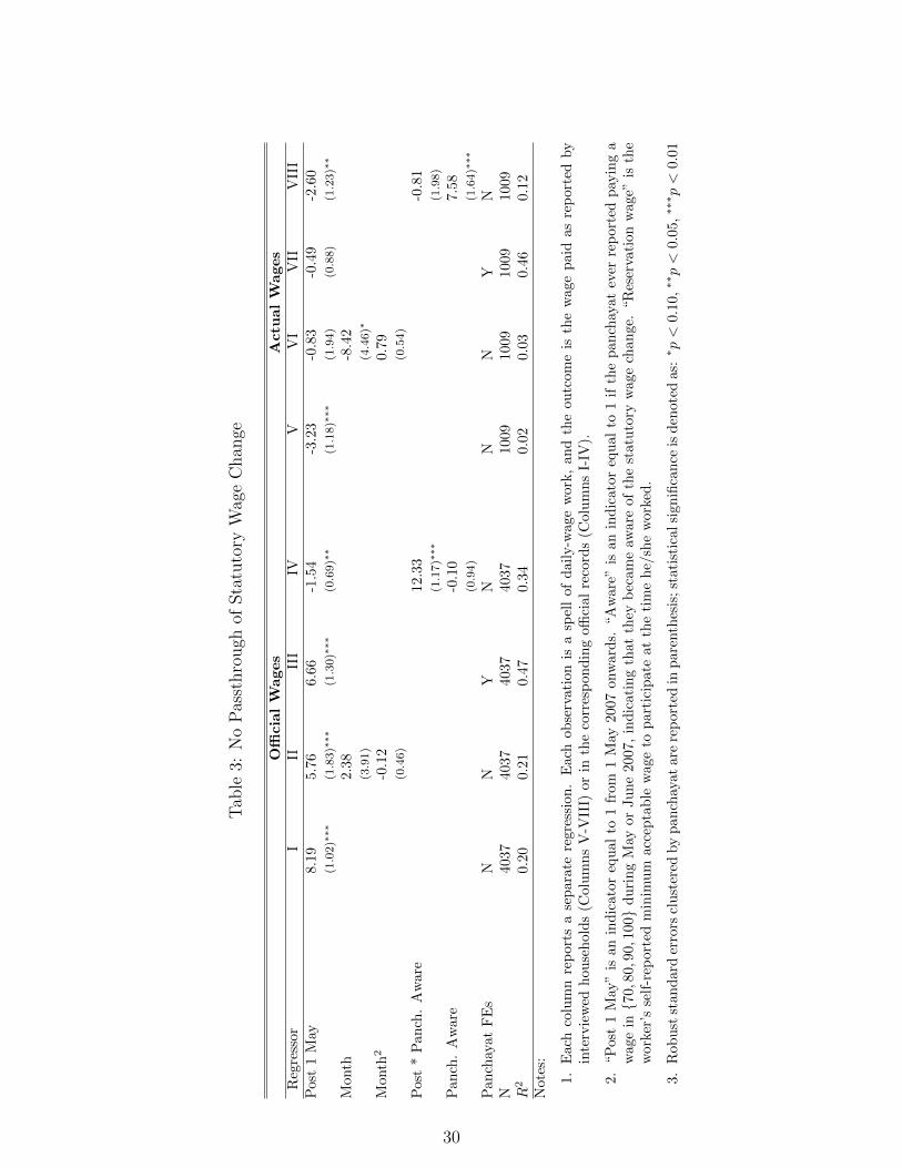
Table 3 provides a more formal statistical analysis of pass-through. In columns V-VIII

observations are spells of daily-wage work as reported by interviewed households, while

12

in columns I-IV they are those reported in the corresponding official records.11 Columns

I-III show that the official wage jumps up significantly after 1 May and that this jump is

abrupt enough to be distinguishable from a quadratic trend (Column II) and widespread

enough to be distinguishable from panachayat fixed effects (Column III).12

One interesting feature of Figure 1 is that while the average wage paid according to

official records increases sharply after 1 May, it does not increase all the way to Rs. 70,

the new minimum wage. The reason for this is that some panchayats continued paying

the older, lower wage rates even after 1 May. The fact that some panchayats did not even

claim to be paying higher wages is something of a puzzle as it essentially means they were

leaving rents on the table. The most plausible explanation is that some panchayats did

not immediately learn about the wage change. Consistent with this view, Columns I and

II of Table 5 show that the post 1 May increase is roughly Rs. 3 larger in panchayats

below median travel time from the block office and from the collector’s office. (These

variables are described in more detail below.) This suggests that when we look at wages

actually received by workers it may be informative to treat “unaware” panchayats as a

control group. Column IV of Table 3 differentiates between panchayats that ever reported

paying a new, higher wage during May or June (the “aware” panchayats) from those that

did not; tautologically, the increase in official wages is concentrated in those that are

aware.13

Columns V-VIII mirror Columns I-IV but using wages actually paid to surveyed house-

holds as the outcome. If marginal leakage were equal to the pre-shock average leakage

rate we would expect to see actual wages increase by the same amount as official wages.

In contrast, and exactly as one would expect from Figure 1, wages are lower after 1 May,

and the effect of shock is estimated at exactly 0 after accounting for quadratic trends or

village effects.

In Column VII we differentiate between panchayats that did or did not ever implement

the statutory wage change. This lets us test for the possibility that some other factor

determining wages changed at the same time as the statutory wage did, offsetting what

would otherwise have been a positive effect. If this were the case we would expect to

see an increase in wages in panchayats that implemented the policy change relative to

those that did not. This is not the case, however: the differential effect is negative and

statistically insignificant. In sum there is strong evidence of 0 pass-through, or 100%

11We categorize a spell of work as occurring on the day it began, so that a spell which overlapped 1 Maywould be attributed to the “pre” period. As a robustness check we also dropped spells (3% each of officialand actual spells) that overlapped the shock date, and this yielded essentially identical results.

12We use months as the time trend variable for comparability to the household-reported spells data, forwhich specific start days within months are not always available due to limited recall. Results for the officialdata are similar using day-of-year trends, however.

13We also ran the same regressions on the restricted set of official spells associated with households thatreported doing some work, and obtained essentially identical results.

13

marginal leakage, on this margin.

5.2 Interpretation: Is Voice a Binding Constraint?

The fact that marginal leakage exceeds average leakage suggests that voice is not a binding

constraint on corruption in the context of the NREGS. In the language of our model, it

implies that the costs of complaining c are large or that the perceived probability π of a

complaint succeeding is low.

To better understand how participants perceive the complaint process we asked them,

“Do you feel you were treated fairly at the job site? Or did you have any problems at

work?” (to which 36% responded that they had had problems) and then “If you did have

any problems, or if a problem were to arise in the future, what would you do about it?”

While this is a broad question that does not specifically refer to issues of under-payment,

it should shed some light on workers’ approach to dealing with wage issues.

The great majority of respondents told us that if they had problems they would

either do nothing (22%), or take up the issue with local panchayat officials or village

elders (74%), the same officials responsible for implementation of the NREGS to begin

with. Only 7% said they would appeal at the Block or District levels, which are the

entities designed by NREGS guidelines for dealing with grievances, and the figure for

workers who had actually experienced problems is still only 13% (Table 4). Among those

who said they would do nothing, the main reasons stated where that complaining would

be in vain (37%) and that complaining would too time-consuming or take too much effort

(53%). 10% indicated fear of retribution as the main deterrent.

One measurable and potentially important component of the costs of complaining are

the costs of traveling to the Block or District office to file a grievance. We have data on

distances and travel times from our survey of village elders. The average village in our

sample is 17km from the corresponding Block office and 38km from the District office, and

average estimated round-trip travel times are 3 hours and 5 hours, respectively.14 There

is of course substantial variation around these means; if travel costs are an important

constraint on voice then we should see a relationship between distance and wage pass-

through. We have already seen that panchayats located closer to block and district

offices saw larger increases in their officially reported wages (Table 5, Columns I and II).

Columns V and VII show, however, that the same is not true for wages actually received.

Actual wage changes are insignificantly different in panchayats close to block offices and

if anything significantly lower in those located close to district offices.

While variation in the probability of successfully complaining is harder to measure,

14These are times using whatever (possibly costly) means of transport the respondent would use. Ata typical walking speed of 3 mph the average round-trip travel times would be 7 hours and 16 hours,respectively.

14

one plausible proxy is the presence of an active non-governmental organization (NGO) in

the village. NGOs in Orissa have formed a loose coalition devoted to monitoring NREGS

implementation and ensuring that participants obtain their entitlements; at least one

NGO is active in 36% of the villages in our sample. Columns III and VII examine whether

the effects of the policy change were different in these villages. Interestingly, while we

find no differential effects on officially reported wages, we do find a significant positive

effect on wages actually received in villages with an active NGO. This is consistent with

the idea that NGOs help program participants hold government accountable. This is not

the only reasonable interpretation, since having an NGO may be correlated with many

other unobservable variables. At a minimum, however, the result establishes that there

exists some such variable that improves accountability, which is encouraging.

A final potential limitation on the effectiveness of complaints is that in the short run

some workers may not have learned about the wage change. We asked respondents what

wages they were owed and whether they knew of any changes in the statutory wage.

72% of the work spells in our sample were done by households that knew that there

had been a change in the daily wage rate, and of these 81% were done by households

that correctly identified the new wage as Rs. 70 per day. However, only 4% of spells

were done by households that correctly identified May 2007 as the month in which the

change took place. Other responses were not obviously bunched around May; the modal

response was to simply identify the year 2007. If awareness of the wage change were

important we would therefore expect to see a gradual upwards trend in wages after 1

May, which is not the case (Figure 1).15 Formally, Column IX of Table 5 shows that

there is no significant tendency for workers from households that learned of the wage

change to receive differentially higher wages after 1 May.

5.3 Interpretation: Is Exit a Binding Constraint?

Given that NREGS workers appear to have little effective voice, we next examine an

alternative recourse: exit.

One interesting piece of circumstantial evidence supporting the exit hypothesis is

visible in Figure 1. During the first month of the study period the mean wage received by

households is actually higher than the mean wage reported in official records. This gap

is driven by a large number of observations from Gajapati district where both prevailing

market wages and household’s reported NREGS wages are relatively high. NGOs working

in this area have reported that officials overpay workers when market wages are high in

order to induce them to participate because this creates scope for further theft in the form

of over-reporting. Of course over-paid workers cannot complain, so for this sub-sample it

15Reinikka and Svensson (2005), Besley and Prat (2006), and Ferraz and Finan (2008) show that providinginformation can help in settings where lack of information is a serious constraint.

15

is clear that exit is the binding constraint.

This example also suggests a more systematic test: if the exit constraint binds then

variation in workers’ outside options should be positively related to the NREGS wage

realizations we observe. This could arise because officials respond to good outside options

with higher wage offers, as in our model, but it would also arise if the distribution of wage

offers stays fixed and only offers above the reservation wage are accepted. In either case

the key to constructing a test is to measure variation in outside options. Private-sector

employment, rather than leisure, appears the be the relevant outside option: when asked

what they would have done if the NREGS wage were below their reservation wage, 96%

of respondents indicated some other form of work as opposed to only 4% who said they

would have waited for a better wage. Higher private sector wages should therefore lead

to higher NREGS wage realizations.

A naive approach to testing this hypothesis would be to regress NREGS wages and

participation on private sector wages. The direction of causality would be unclear, how-

ever; indeed the standard view of employment guarantee schemes is that they act as a

binding floor on private sector wages. To circumvent this simultaneity issue we exploit

variation in local factor endowments. If a village endowed with cultivatable land T and la-

bor L produces output Y = F (T, L) then the competitive real wage will be w = FL(T, L);

assuming decreasing returns to labor and land-labor complementarity this wage will be

decreasing in the labor endowment and increasing in the land endowment.

We matched our survey data to records from the 2001 Census on the stock of cultivat-

able land and the total population at the Gram Panchayat level. Unlike contemporaneous

market wages these quantities were pre-determined prior to the launch of the NREGA

in 2005, so there is no concern about reverse causality. Relative factor endowments vary

substantially, due either to historical demographic shocks (if workers are immobile) or

to variation in location-specific amenities that compensate for real wage differentials (if

workers are mobile). The chief concern is that that this variation is correlated with other

determinants of worker’s “residual” bargaining power, represented as α in our model (see

Equation 3). The fact that none of the statutory wage increase was passed through to

workers suggests that α = 0; we will nevertheless check the sensitivity of our results to

controlling for variables that might plausibly capture variation in α in an effort to address

this concern.

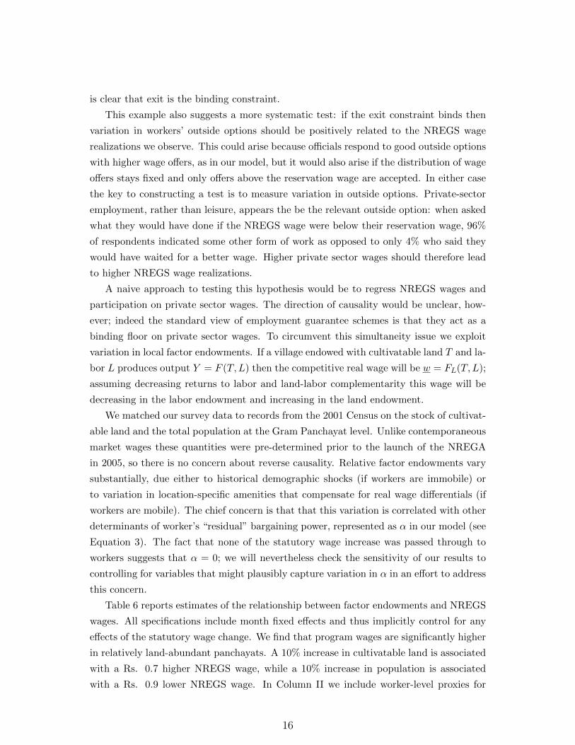
Table 6 reports estimates of the relationship between factor endowments and NREGS

wages. All specifications include month fixed effects and thus implicitly control for any

effects of the statutory wage change. We find that program wages are significantly higher

in relatively land-abundant panchayats. A 10% increase in cultivatable land is associated

with a Rs. 0.7 higher NREGS wage, while a 10% increase in population is associated

with a Rs. 0.9 lower NREGS wage. In Column II we include worker-level proxies for

16

bargaining power; we find that men, non-minorities, and workers paid through banks

receive significantly higher wages, reflecting either stronger bargaining power or better

outside options. In Column III we control for village-level predictors of bargaining power,

and in Column IV we include both control sets. The coefficients on land and population

remain strongly significant across all specifications and fall by at most 30% relative to

the uncontrolled model.

In addition to supporting the exit view of NREGS wage determination these results

have interesting distributional implications: evidently NREGS wages are regressive across

labor markets, paying out higher wages in markets where wages were higher to begin with.

Reinikka and Svensson (2004) also find regressive leakage in funding flows to Ugandan

schools, which they attribute to variation in communities effective voice.

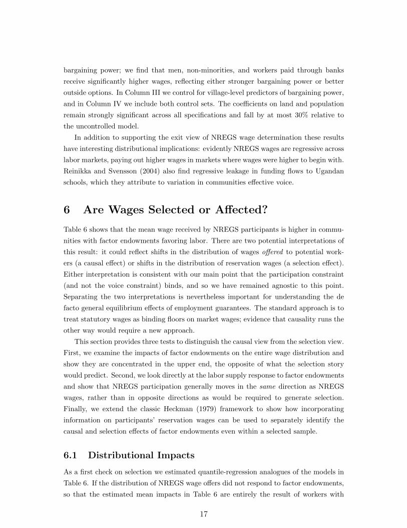
6 Are Wages Selected or Affected?

Table 6 shows that the mean wage received by NREGS participants is higher in commu-

nities with factor endowments favoring labor. There are two potential interpretations of

this result: it could reflect shifts in the distribution of wages offered to potential work-

ers (a causal effect) or shifts in the distribution of reservation wages (a selection effect).

Either interpretation is consistent with our main point that the participation constraint

(and not the voice constraint) binds, and so we have remained agnostic to this point.

Separating the two interpretations is nevertheless important for understanding the de

facto general equilibrium effects of employment guarantees. The standard approach is to

treat statutory wages as binding floors on market wages; evidence that causality runs the

other way would require a new approach.

This section provides three tests to distinguish the causal view from the selection view.

First, we examine the impacts of factor endowments on the entire wage distribution and

show they are concentrated in the upper end, the opposite of what the selection story

would predict. Second, we look directly at the labor supply response to factor endowments

and show that NREGS participation generally moves in the same direction as NREGS

wages, rather than in opposite directions as would be required to generate selection.

Finally, we extend the classic Heckman (1979) framework to show how incorporating

information on participants’ reservation wages can be used to separately identify the

causal and selection effects of factor endowments even within a selected sample.

6.1 Distributional Impacts

As a first check on selection we estimated quantile-regression analogues of the models in

Table 6. If the distribution of NREGS wage offers did not respond to factor endowments,

so that the estimated mean impacts in Table 6 are entirely the result of workers with

17

low NREGS wage offers selecting out, then we would expect to see impacts concentrated

in the lower quantiles of the distribution. Figure 2 plots the estimated coefficients on

our two factor endowment measures from a series of quantile regressions at each decile,

including month dummies. Evidently the effects are concentrated in the upper, not lower,

end of the distribution.

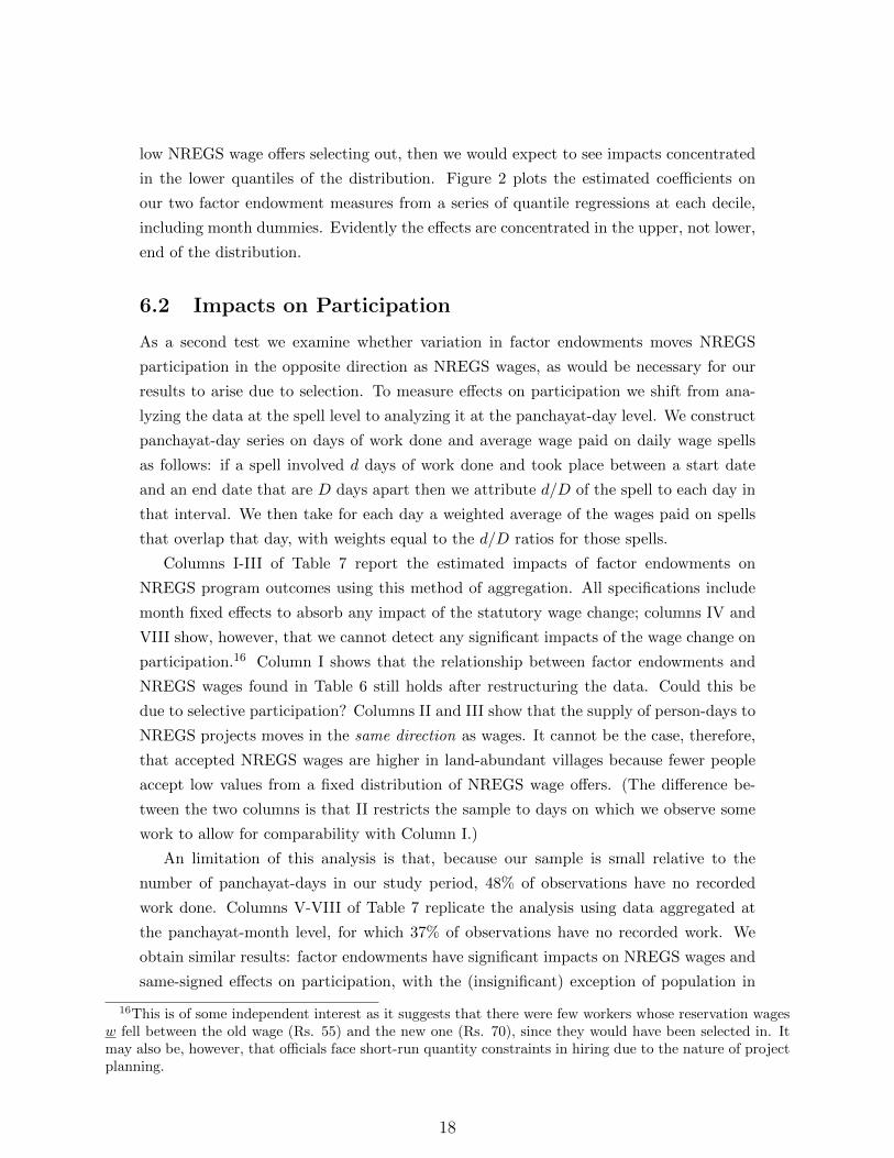
6.2 Impacts on Participation

As a second test we examine whether variation in factor endowments moves NREGS

participation in the opposite direction as NREGS wages, as would be necessary for our

results to arise due to selection. To measure effects on participation we shift from ana-

lyzing the data at the spell level to analyzing it at the panchayat-day level. We construct

panchayat-day series on days of work done and average wage paid on daily wage spells

as follows: if a spell involved d days of work done and took place between a start date

and an end date that are D days apart then we attribute d/D of the spell to each day in

that interval. We then take for each day a weighted average of the wages paid on spells

that overlap that day, with weights equal to the d/D ratios for those spells.

Columns I-III of Table 7 report the estimated impacts of factor endowments on

NREGS program outcomes using this method of aggregation. All specifications include

month fixed effects to absorb any impact of the statutory wage change; columns IV and

VIII show, however, that we cannot detect any significant impacts of the wage change on

participation.16 Column I shows that the relationship between factor endowments and

NREGS wages found in Table 6 still holds after restructuring the data. Could this be

due to selective participation? Columns II and III show that the supply of person-days to

NREGS projects moves in the same direction as wages. It cannot be the case, therefore,

that accepted NREGS wages are higher in land-abundant villages because fewer people

accept low values from a fixed distribution of NREGS wage offers. (The difference be-

tween the two columns is that II restricts the sample to days on which we observe some

work to allow for comparability with Column I.)

An limitation of this analysis is that, because our sample is small relative to the

number of panchayat-days in our study period, 48% of observations have no recorded

work done. Columns V-VIII of Table 7 replicate the analysis using data aggregated at

the panchayat-month level, for which 37% of observations have no recorded work. We

obtain similar results: factor endowments have significant impacts on NREGS wages and

same-signed effects on participation, with the (insignificant) exception of population in

16This is of some independent interest as it suggests that there were few workers whose reservation wagesw fell between the old wage (Rs. 55) and the new one (Rs. 70), since they would have been selected in. Itmay also be, however, that officials face short-run quantity constraints in hiring due to the nature of projectplanning.

18

Column VI.

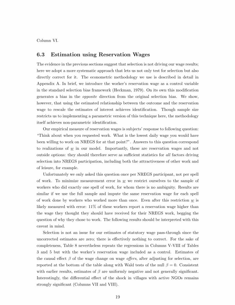
6.3 Estimation using Reservation Wages

The evidence in the previous sections suggest that selection is not driving our wage results;

here we adopt a more systematic approach that lets us not only test for selection but also

directly correct for it. The econometric methodology we use is described in detail in

Appendix A. In brief, we introduce the worker’s reservation wage as a control variable

in the standard selection bias framework (Heckman, 1979). On its own this modification

generates a bias in the opposite direction from the original selection bias. We show,

however, that using the estimated relationship between the outcome and the reservation

wage to rescale the estimates of interest achieves identification. Though sample size

restricts us to implementing a parametric version of this technique here, the methodology

itself achieves non-parametric identification.

Our empirical measure of reservation wages is subjects’ response to following question:

“Think about when you requested work. What is the lowest daily wage you would have

been willing to work on NREGS for at that point?”. Answers to this question correspond

to realizations of w in our model. Importantly, these are reservation wages and not

outside options: they should therefore serve as sufficient statistics for all factors driving

selection into NREGS participation, including both the attractiveness of other work and

of leisure, for example.

Unfortunately we only asked this question once per NREGS participant, not per spell

of work. To minimize measurement error in w we restrict ourselves to the sample of

workers who did exactly one spell of work, for whom there is no ambiguity. Results are

similar if we use the full sample and impute the same reservation wage for each spell

of work done by workers who worked more than once. Even after this restriction w is

likely measured with error: 11% of these workers report a reservation wage higher than

the wage they thought they should have received for their NREGS work, begging the

question of why they chose to work. The following results should be interpreted with this

caveat in mind.

Selection is not an issue for our estimates of statutory wage pass-through since the

uncorrected estimates are zero; there is effectively nothing to correct. For the sake of

completeness, Table 8 nevertheless repeats the regressions in Columns V-VIII of Tables

3 and 5 but with the worker’s reservation wage included as a control. Estimates of

the causal effect β of the wage change on wage offers, after adjusting for selection, are

reported at the bottom of the table along with Wald tests of the null β = 0. Consistent

with earlier results, estimates of β are uniformly negative and not generally significant.

Interestingly, the differential effect of the shock in villages with active NGOs remains

strongly significant (Columns VII and VIII).

19

Table 9 performs an analogous exercise for our estimates of the effect of factor endow-

ments on NREGS wage offers. Panel A simply repeats the uncorrected results reported in

Table 6 for our new, restricted estimation sample. Panel B re-estimates the same models

but includes worker’s reservation wage as an additional control. Recall that this specifi-

cation will bias the estimates of interest towards 0 in the presence of selection (Equation

11). As expected the point estimates on our labor market shock indicators are smaller

than those in Panel A, but they remain statistically significant.

In Panel C we calculate the implied causal impact of these variables on program wage

offers, adjusting for selection. Our estimates are similar and on average slightly larger

than the uncorrected estimates in Panel A; they confirm that officials offer significantly

higher wages in panchayats more abundantly endowed with land and less abundantly

endowed with labor. Both results are highly significant across all specifications. Together

they support the claim that labor market conditions have a causal effect on wage offers,

and not only on participation.

7 Conclusion

Social policy-making in developing countries requires an understanding of corruption, and

marginal rates of leakage are a particularly important input into decision-making. We

provide the first estimates of marginal leakage for an important social protection program,

India’s National Rural Employment Guarantee Scheme. We estimate that marginal leak-

age with respect to an increase in the statutory daily wage due to workers was 100%: none

of the wage increase was passed through to workers. Auxiliary evidence suggests that

this is because the threat of exit to the private sector, and not the threat of complaining

to higher-ups, is the binding constraint on wage under-payment.

Our analysis was motivated by the question of optimal redistribution. To see what

the results imply for redistributive policy we can return to Equation 1. A planner who

believed that marginal leakage in the NREGS was equal to our pre-shock estimate of

average leakage, 75%, would have thought a wage increase desirable provided the welfare

weight on recipients was at least 4 times the marginal cost of public funds. In contrast,

a planner who knew that marginal leakage would be 100% would never increase the

statutory wage. As this illustrates, distinguishing marginal from average leakage can

have important policy consequences.

20

References

Atanassova, Antonia, Marianne Bertrand, Sendhil Mullainathan, and Paul

Niehaus, “Targeting with Agents: Theory and Evidence for India’s Below Poverty

Line Cards,” 2010. mimeo, UC San Diego.

Atkinson, Anthony B and N H Stern, “Pigou, Taxation and Public Goods,” Review

of Economic Studies, January 1974, 41 (1), 119–28.

Basu, Arnab K., Nancy H. Chau, and Ravi Kanbur, “A theory of employment

guarantees: Contestability, credibility and distributional concerns,” Journal of Public

Economics, April 2009, 93 (3-4), 482–497.

Besley, Timothy and Andrea Prat, “Handcuffs for the Grabbing Hand? Media

Capture and Government Accountability,” American Economic Review, June 2006, 96

(3), 720–736.

and Stephen Coate, “Workfare versus Welfare: Incentive Arguments for Work Re-

quirements in Poverty-Alleviation Programs,” The American Economic Review, 1992,

82 (1), 249–261.

and Torsten Persson, “The Origins of State Capacity: Property Rights, Taxation,

and Politics,” American Economic Review, September 2009, 99 (4), 1218–44.

and , “State Capacity, Conflict, and Development,” Econometrica, 01 2010, 78 (1),

1–34.

Chattopadhyay, Raghabendra and Esther Duflo, “Women as Policy Makers: Evi-

dence from a Randomized Policy Experiment in India,” Econometrica, 09 2004, 72 (5),

1409–1443.

Chaudhury, Nazmul, Jeffrey Hammer, Michael Kremer, Karthik Muralid-

haran, and F. Halsey Rogers, “Missing in Action: Teacher and Health Worker

Absence in Developing Countries,” Journal of Economic Perspectives, Winter 2006, 20

(1), 91–116.

Dahlby, Bev, The Marginal Cost of Public Funds: Theory and Applications, Cambridge,

MA: MIT Press, 2008.

Das, Vidhya and Pramod Pradhan, “Illusions of Change,” Economic and Political

Weekly, August 2007, 42 (32).

21

Diamond, Peter A and James A Mirrlees, “Optimal Taxation and Public Pro-

duction: I–Production Efficiency,” American Economic Review, March 1971, 61 (1),

8–27.

Ferraz, Claudio and Frederico Finan, “Exposing Corrupt Politicians: The Effects of

Brazil’s Publicly Released Audits on Electoral Outcomes,” The Quarterly Journal of

Economics, 05 2008, 123 (2), 703–745.

, Fred Finan, and Diana Moreira, “Corrupting Learning: Evidence from Missing

Federal Education Funds in Brazil,” Technical Report, UC Berkeley April 2010.

Gordon, Roger and Wei Li, “Tax structures in developing countries: Many puzzles

and a possible explanation,” Journal of Public Economics, August 2009, 93 (7-8), 855–

866.

Heckman, James J, “Sample Selection Bias as a Specification Error,” Econometrica,

January 1979, 47 (1), 153–61.

Hirschmann, Albert, Exit, Voice, and Loyalty: Responses to Declines in Firms, Orga-

nizations, and States, Cambridge, MA: Harvard University, 1970.

Hunt, Jennifer and Sonia Laszlo, “Bribery: Who Pays, Who Refuses, What Are the

Payoffs?,” NBER Working Papers 11635, National Bureau of Economic Research, Inc

September 2005.

Keen, Michael, “VAT, tariffs, and withholding: Border taxes and informality in devel-

oping countries,” Journal of Public Economics, October 2008, 92 (10-11), 1892–1906.

Niehaus, Paul and Sandip Sukhtankar, “Corruption Dynamics: the Golden Goose

Effect,” Technical Report, UCSD February 2010.

Olken, Benjamin A., “Corruption and the costs of redistribution: Micro evidence from

Indonesia,” Journal of Public Economics, May 2006, 90 (4-5), 853–870.

, “Monitoring Corruption: Evidence from a Field Experiment in Indonesia,” Journal

of Political Economy, April 2007, 115 (2), 200–249.

Olken, Benjamin and Monica Singhal, “Informal Taxation,” Technical Report, Har-

vard University January 2010.

Pigou, A.C., A Study in Public Finance, New York: St. Martin’s Press, Inc., 1960.

Programme Evaluation Organization, “Performance Evaluation of Targeted Public

Distribution System,” Technical Report, Planning Commission, Government of India

March 2005.

22

Ravallion, Martin, “Market Responses to Anti-Hunger Policies: Effects on Wages,

Prices, and Employment,” November 1987. World Institute for Development Economics

Research WP28.

, Gaurav Datt, and Shubham Chaudhuri, “Does Maharashtra’s Employment

Guarantee Scheme Guarantee Employment? Effects of the 1988 Wage Increase,” Eco-

nomic Development and Cultural Change, January 1993, 41 (2), 251–75.

Reinikka, Ritva and Jakob Svensson, “Local Capture: Evidence From a Central

Government Transfer Program in Uganda,” The Quarterly Journal of Economics, May

2004, 119 (2), 678–704.

and , “Fighting Corruption to Improve Schooling: Evidence from a Newspaper

Campaign in Uganda,” Journal of the European Economic Association, 04/05 2005, 3

(2-3), 259–267.

Stiglitz, Joseph E and P Dasgupta, “Differential Taxation, Public Goods and Eco-

nomic Efficiency,” Review of Economic Studies, April 1971, 38 (114), 151–74.

Svensson, Jakob, “Who Must Pay Bribes And How Much? Evidence From A Cross

Section Of Firms,” The Quarterly Journal of Economics, February 2003, 118 (1), 207–

230.

23

A Correcting for Selection using Reservation Wages

To characterize the selection problem let s be any variable predicted to affect program

wage offers w; in practice this will be a measure of factor endowments or the statutory

wage. Let

w = f(s) + u (8)

describe the relationship between official wage offers and this variable; we are interested

in estimating f(·). Similarly let a worker’s reservation wage be

w = g(s) + v (9)

The error terms u and v are defined to be uncorrelated with s. If s is the statutory wage

then we expect g(·) to be invariant to it, while if s is a factor endowment then g(·) should

respond to it. In either case the selection problem is that we observe (w,w) only if w ≥ wso that the worker chooses to work on the NREGS project. Let d = 1(w ≥ w) indicate

this event. If we ignore this and estimate the conditional expectation of w given s we

obtain

E[w|s, d = 1] = f(s) + E[u|u ≥ g(s)− f(s) + v] (10)

where the second term captures selection bias (Heckman, 1979). We expect a bias towards

zero for innovations to the statutory wage: for example, if the distribution of program

wage offers shifts up there will be selection into the sample of workers whose (new) offers

are just above their reservation wages. For factor endowments the bias cannot be signed

a priori, though our model predicts that exogenous changes in w should pass through less

than one-for-one to w in which case we expect |g′| > |f ′| and thus a bias away from zero

in OLS estimates of f ′.

To identify f we exploit our data on reservation wages w. Consider

E[w|s, w, d = 1] = f(s) + E[u|u ≥ w − f(s)] (11)

≡ f(s) + h(w − f(s)) (12)

where the second equation implicitly defines h(·) as a conditional expectation function.

Differentiating with respect to s shows that this equation identifies f ′(s)(1−h′(w−f(s))).

Because h′ ≥ 0 this quantity will generally be biased as an estimator of f ′, with the bias

tending towards 0 or even flipping the sign of the estimate if h′ > 1. Simply controlling

for the reservation wage is therefore inappropriate. Variation in the reservation wage,

however, can be used to identify h′ as

h′(x) =∂

∂wE[w|s, w, d = 1] (13)

24

This done we can correct for the bias in (11) and identify f ′ as

f ′(s) =∂∂sE[w|s, w, d = 1]

1− ∂∂wE[w|s, w, d = 1]

(14)

Intuitively, the OLS estimate must be scaled to adjust for selection bias. This allows us

to construct tests of the null hypothesis that s has no effect on the wage offer w. When

s is a factor endowment we would also like to quantify the relative sensitivity of w and w

to s and then calculate pass-through ratios. Differentiating (10) and re-arranging yields

g′(s) = f ′(s) +∂∂sE[w|s, d = 1]− f ′(s)

E[h′(g(s)− f(s) + v)|s, d = 1](15)

Given that f ′ and h′ are identified this identifies g′ up to the distribution of v. If we

accept the linear approximation h′ = γ then

g′(s) =

(1− 1

γ

)f ′(s) +

1

γ

∂

∂sE[w|s, d = 1] (16)

is identified. Given our limited sample size we will use linear approximations to all three

functions: f(s) = βs, g(s) = αs, and h(x) = γx. In this case

E[w|s, w, d = 1] = (1− γ)βs+ γw (17)

E[w|s, d = 1] = [(1− γ)β + γα]s (18)

and consistent estimators of the coefficients (β, α, γ) can be obtained by running the

reduced-form regressions

E[w|s, w, d = 1] = πss+ πww (19)

E[w|s, d = 1] = θss (20)

and then calculating

β̂ =π̂s

1− π̂w(21)

γ̂ = π̂w (22)

α̂ =θ̂s − π̂sπ̂w

(23)

This is the approach we implement in the text.

25

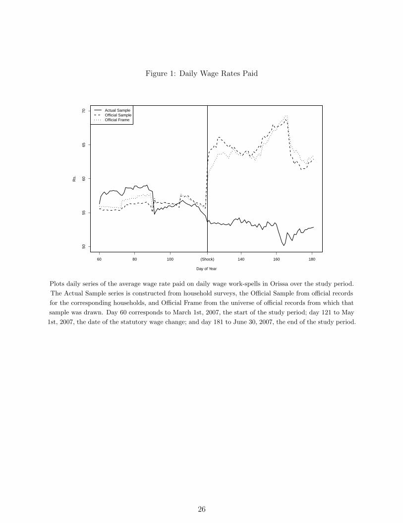
Figure 1: Daily Wage Rates Paid50

5560

6570

Day of Year

Rs.

Actual SampleOfficial SampleOfficial Frame

60 80 100 140 160 180(Shock)

Plots daily series of the average wage rate paid on daily wage work-spells in Orissa over the study period.

The Actual Sample series is constructed from household surveys, the Official Sample from official records

for the corresponding households, and Official Frame from the universe of official records from which that

sample was drawn. Day 60 corresponds to March 1st, 2007, the start of the study period; day 121 to May

1st, 2007, the date of the statutory wage change; and day 181 to June 30, 2007, the end of the study period.

26

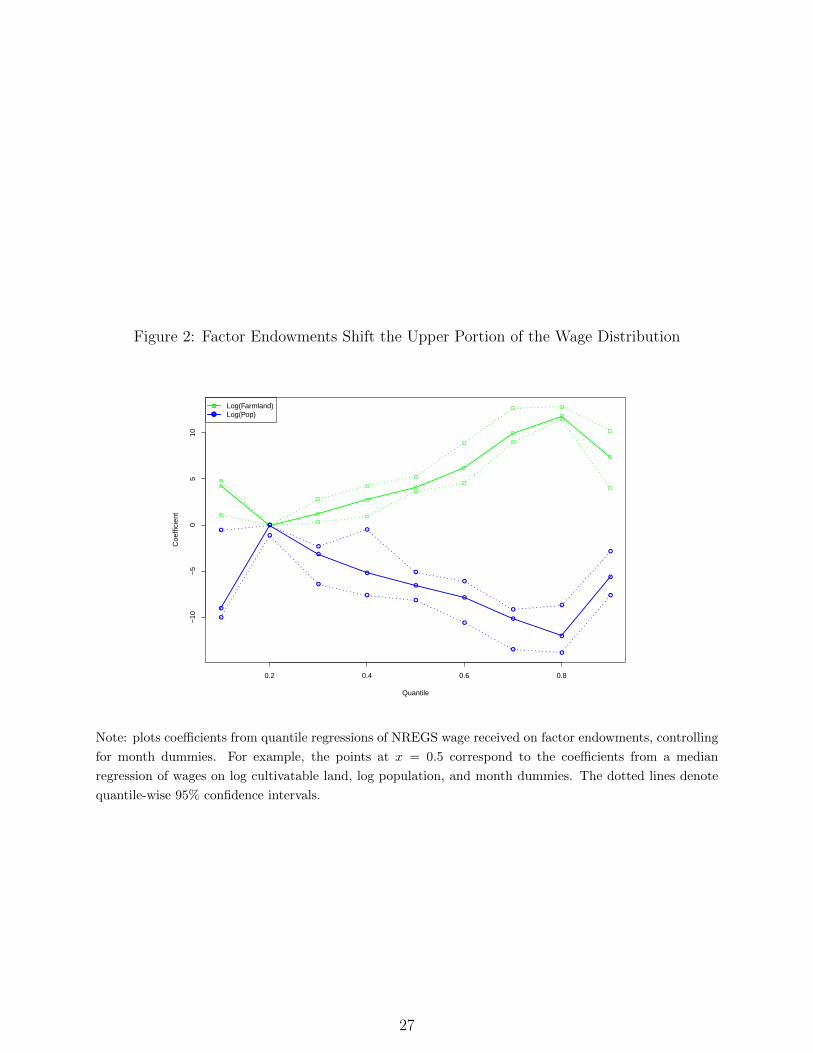
Figure 2: Factor Endowments Shift the Upper Portion of the Wage Distribution

0.2 0.4 0.6 0.8

−10

−5

05

10

Quantile

Coe

ffici

ent

●

●

●

●

●

●

●

●

●

●

●

●

●●

●

●●

●

●●

●

●

●

●

●●

●

●

Log(Farmland)Log(Pop)

Note: plots coefficients from quantile regressions of NREGS wage received on factor endowments, controlling

for month dummies. For example, the points at x = 0.5 correspond to the coefficients from a median

regression of wages on log cultivatable land, log population, and month dummies. The dotted lines denote

quantile-wise 95% confidence intervals.

27

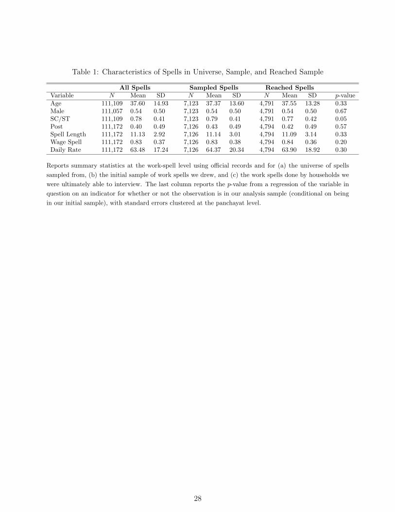
Table 1: Characteristics of Spells in Universe, Sample, and Reached Sample

All Spells Sampled Spells Reached SpellsVariable N Mean SD N Mean SD N Mean SD p-valueAge 111,109 37.60 14.93 7,123 37.37 13.60 4,791 37.55 13.28 0.33Male 111,057 0.54 0.50 7,123 0.54 0.50 4,791 0.54 0.50 0.67SC/ST 111,109 0.78 0.41 7,123 0.79 0.41 4,791 0.77 0.42 0.05Post 111,172 0.40 0.49 7,126 0.43 0.49 4,794 0.42 0.49 0.57Spell Length 111,172 11.13 2.92 7,126 11.14 3.01 4,794 11.09 3.14 0.33Wage Spell 111,172 0.83 0.37 7,126 0.83 0.38 4,794 0.84 0.36 0.20Daily Rate 111,172 63.48 17.24 7,126 64.37 20.34 4,794 63.90 18.92 0.30

Reports summary statistics at the work-spell level using official records and for (a) the universe of spells

sampled from, (b) the initial sample of work spells we drew, and (c) the work spells done by households we

were ultimately able to interview. The last column reports the p-value from a regression of the variable in

question on an indicator for whether or not the observation is in our analysis sample (conditional on being

in our initial sample), with standard errors clustered at the panchayat level.

28

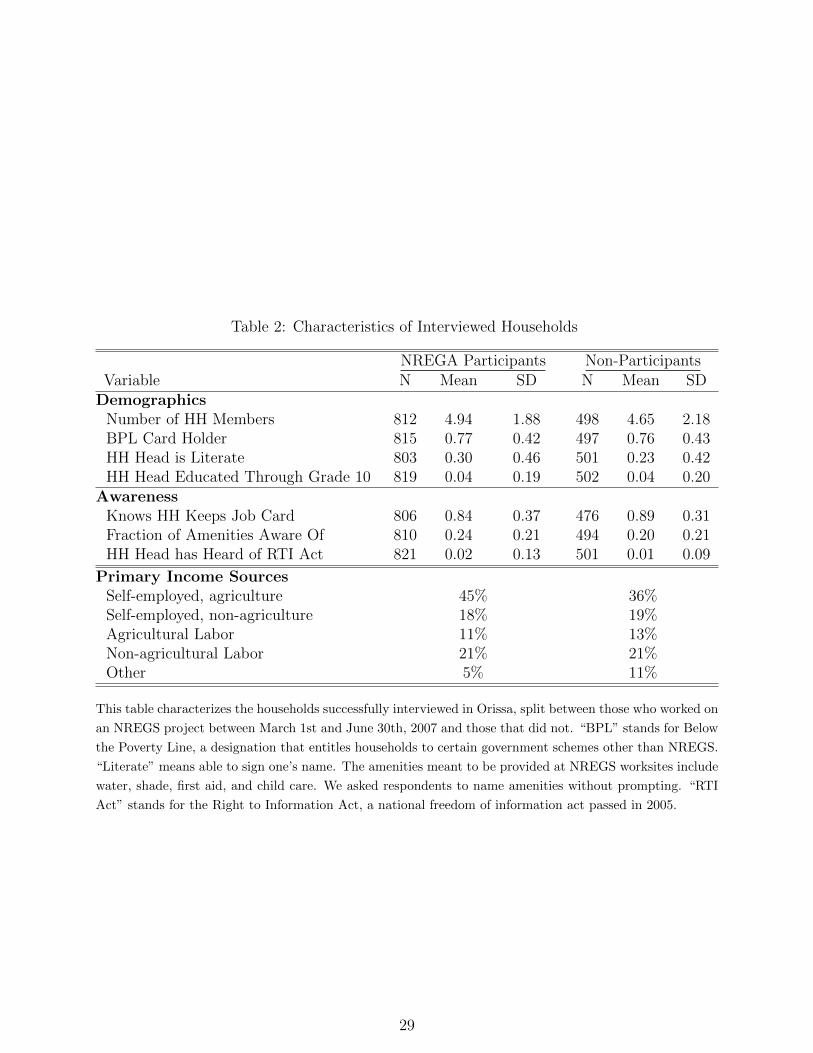
Table 2: Characteristics of Interviewed Households

NREGA Participants Non-ParticipantsVariable N Mean SD N Mean SD

DemographicsNumber of HH Members 812 4.94 1.88 498 4.65 2.18BPL Card Holder 815 0.77 0.42 497 0.76 0.43HH Head is Literate 803 0.30 0.46 501 0.23 0.42HH Head Educated Through Grade 10 819 0.04 0.19 502 0.04 0.20

AwarenessKnows HH Keeps Job Card 806 0.84 0.37 476 0.89 0.31Fraction of Amenities Aware Of 810 0.24 0.21 494 0.20 0.21HH Head has Heard of RTI Act 821 0.02 0.13 501 0.01 0.09

Primary Income SourcesSelf-employed, agriculture 45% 36%Self-employed, non-agriculture 18% 19%Agricultural Labor 11% 13%Non-agricultural Labor 21% 21%Other 5% 11%

This table characterizes the households successfully interviewed in Orissa, split between those who worked on

an NREGS project between March 1st and June 30th, 2007 and those that did not. “BPL” stands for Below

the Poverty Line, a designation that entitles households to certain government schemes other than NREGS.

“Literate” means able to sign one’s name. The amenities meant to be provided at NREGS worksites include

water, shade, first aid, and child care. We asked respondents to name amenities without prompting. “RTI

Act” stands for the Right to Information Act, a national freedom of information act passed in 2005.

29

Tab

le3:

No

Pas

sthro

ugh

ofSta

tuto

ryW

age

Chan

ge

Offi

cia

lW

ages

Actu

al

Wages

Reg

ress

orI

IIII

IIV

VV

IV

IIV

III

Pos

t1

May

8.19

5.76

6.6

6-1

.54

-3.2

3-0

.83

-0.4

9-2

.60

(1.02)∗

∗∗(1.83)∗

∗∗(1.30)∗

∗∗(0.69)∗

∗(1.18)∗

∗∗(1.94)

(0.88)

(1.23)∗

∗

Mon

th2.

38-8

.42

(3.91)

(4.46)∗

Mon

th2

-0.1

20.7

9(0.46)

(0.54)

Pos

t*

Pan

ch.

Aw

are

12.3

3-0

.81

(1.17)∗

∗∗(1.98)

Pan

ch.

Aw

are

-0.1

07.5

8(0.94)

(1.64)∗

∗∗

Pan

chay

atF

Es

NN

YN

NN

YN

N40

3740

374037

4037

1009

1009

1009

1009

R2

0.20

0.21

0.4

70.3

40.0

20.0

30.4

60.1

2N

otes

:

1.E

ach

colu

mn

rep

orts

ase

par

ate

regr

essi

on.

Eac

hob

serv

ati

on

isa

spel

lof

dail

y-w

age

work

,an

dth

eou

tcom

eis

the

wage

paid

as

rep

ort

edby

inte

rvie

wed

hou

seh

old

s(C

olu

mn

sV

-VII

I)or

inth

eco

rres

pon

din

goffi

cial

reco

rds

(Colu

mn

sI-

IV).

2.“P

ost

1M

ay”

isan

ind

icat

oreq

ual

to1

from

1M

ay2007

onw

ard

s.“A

ware

”is

an

ind

icato

req

ual

to1

ifth

ep

an

chay

at

ever

rep

ort

edp

ayin

ga

wag

ein{7

0,8

0,9

0,1

00}

du

rin

gM

ayor

Ju

ne

2007

,in

dic

ati

ng

that

they

bec

am

eaw

are

of

the

statu

tory

wage

chan

ge.

“R

eser

vati

on

wage”

isth

ew

orke

r’s

self

-rep

orte

dm

inim

um

acce

pta

ble

wag

eto

part

icip

ate

at

the

tim

eh

e/sh

ew

ork

ed.

3.R

obu

stst

and

ard

erro

rscl

ust

ered

by

pan

chay

atar

ere

port

edin

pare

nth

esis

;st

ati

stic

alsi

gn

ifica

nce

isd

enote

das:∗ p<

0.10,∗∗p<

0.05,∗∗∗ p<

0.01

30

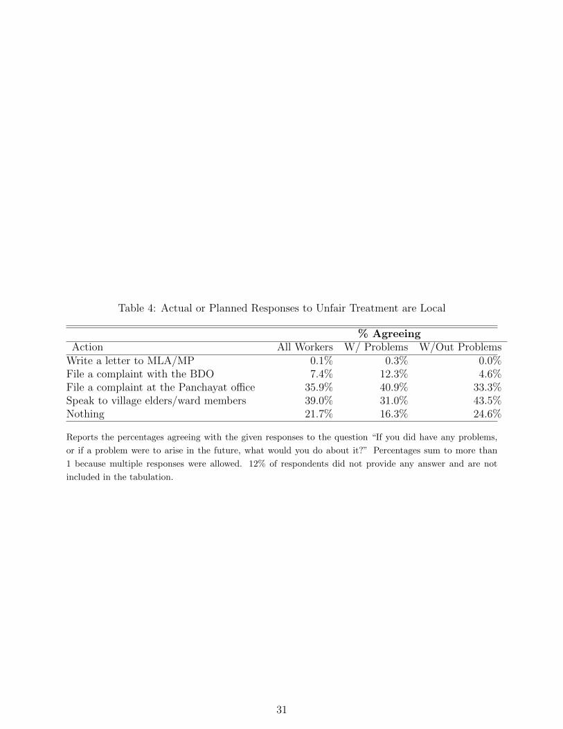
Table 4: Actual or Planned Responses to Unfair Treatment are Local

% AgreeingAction All Workers W/ Problems W/Out Problems

Write a letter to MLA/MP 0.1% 0.3% 0.0%File a complaint with the BDO 7.4% 12.3% 4.6%File a complaint at the Panchayat office 35.9% 40.9% 33.3%Speak to village elders/ward members 39.0% 31.0% 43.5%Nothing 21.7% 16.3% 24.6%

Reports the percentages agreeing with the given responses to the question “If you did have any problems,

or if a problem were to arise in the future, what would you do about it?” Percentages sum to more than

1 because multiple responses were allowed. 12% of respondents did not provide any answer and are not

included in the tabulation.

31

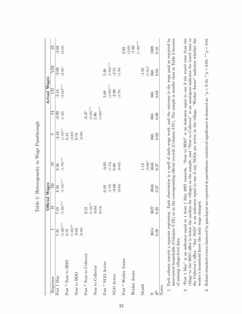
Tab

le5:

Het

erog

enei

tyin

Wag

eP

asst

hro

ugh

Offi

cia

lW

ages

Actu

al

Wages

Reg

ress

orI

IIII

IIV

VV

IV

IIV

III

IXP

ost

1M

ay7.

357.

188.5

66.5

6-3

.44

-0.9

9-5

.44

-2.0

9-3

.68

(1.20)∗

∗∗(1.28)∗

∗∗(1.12)∗

∗∗(1.78)∗

∗∗(1.45)∗

∗(1.32)

(1.62)∗

∗∗(2.38)

(2.42)

Pos

t*

Nea

rto

BD

O3.

180.4

4(1.62)∗

∗(2.63)

Nea

rto

BD

O-0

.61

0.7

3(0.59)

(2.09)

Pos

t*

Nea

rto

Col

lect

or3.

12-6

.37

(1.48)∗

∗(2.22)∗

∗∗

Nea

rto

Col

lect

or-0

.64

5.9

0(0.54)

(1.60)∗

∗∗

Pos

t*

NG

OA

ctiv

e0.1

9-0

.05

5.6

95.4

9(1.76)

(1.73)

(1.93)∗

∗∗(1.94)∗

∗∗

NG

OA

ctiv

e-0

.06

0.0

0-2

.90

-2.5

1(0.63)

(0.63)

(1.78)

(1.76)

Pos

t*

Wor

ker

Aw

are

2.0

2(2.62)

Wor

ker

Aw

are

-7.8

0(1.40)∗

∗∗

Mon

th1.1

2-1

.91

(0.66)∗

(1.01)∗

N36

1436

273646

3646

860

860

860

860

1009

R2

0.28

0.28

0.2

70.2

70.0

20.0

60.0

30.0

40.1

0N

otes

:

1.E

ach

colu

mn

rep

orts

ase

par

ate

regr

essi

on.

Eac

hob

serv

ati

on

isa

spel

lof

dail

y-w

age

work

,an

dth

eou

tcom

eis

the

wage

paid

as

rep

ort

edby

inte

rvie

wed

hou

seh

old

s(C

olu

mn

sV

-IX

)or

inth

eco

rres

pon

din

goffi

cial

reco

rds

(Colu

mn

sI-

IV).

Th

esa

mp

leis

small

erth

an

inT

ab

le3

bec

au

seof

mis

sin

gvil

lage

-lev

eld

ata.

2.“P

ost

1M

ay”

isan

ind

icat

oreq

ual

to1

from

1M

ay2007

onw

ard

s.“N

ear

toB

DO

”is

an

ind

icato

req

ual

toon

eif

the

trav

elti

me

from

the

vil

lage

toth

eB

DO

office

isb

elow

the

med

ian

for

vil

lages

inth

esa

mp

le,

an

d“N

ear

toC

oll

ecto

r”is

an

an

alo

gou

sin

dic

ato

rfo

rtr

avel

tim

eto

the

Col

lect

or’s

office

.“A

ny

NG

O”

isan

ind

icat

or

equ

al

toon

eif

any

NG

Os

are

act

ive

inth

evil

lage.

“W

ork

erA

ware

”in

dic

ate

sw

het

her

the

wor

ker’

sh

ouse

hol

dkn

ewth

ed

aily

wag

ech

ange

d.

3.R

obu

stst

and

ard

erro

rscl

ust

ered

by

pan

chay

atar

ere

port

edin

pare

nth

esis

;st

ati

stic

alsi

gn

ifica

nce

isd

enote

das:∗ p<

0.10,∗∗p<

0.05,∗∗∗ p<

0.01

32

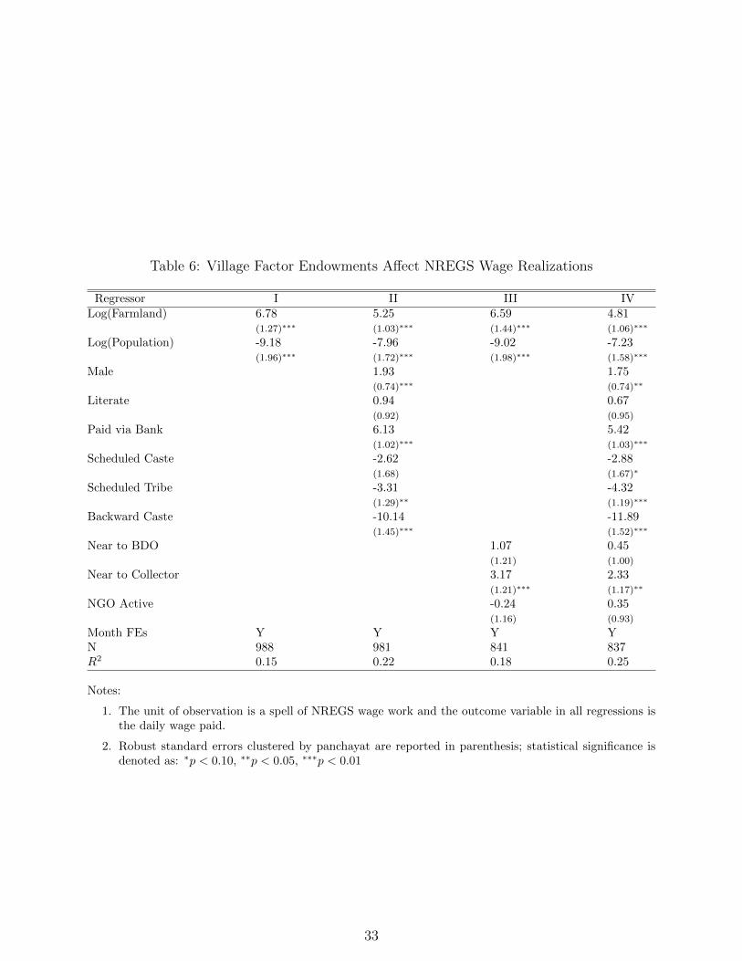
Table 6: Village Factor Endowments Affect NREGS Wage Realizations

Regressor I II III IVLog(Farmland) 6.78 5.25 6.59 4.81

(1.27)∗∗∗ (1.03)∗∗∗ (1.44)∗∗∗ (1.06)∗∗∗

Log(Population) -9.18 -7.96 -9.02 -7.23(1.96)∗∗∗ (1.72)∗∗∗ (1.98)∗∗∗ (1.58)∗∗∗

Male 1.93 1.75(0.74)∗∗∗ (0.74)∗∗

Literate 0.94 0.67(0.92) (0.95)

Paid via Bank 6.13 5.42(1.02)∗∗∗ (1.03)∗∗∗

Scheduled Caste -2.62 -2.88(1.68) (1.67)∗

Scheduled Tribe -3.31 -4.32(1.29)∗∗ (1.19)∗∗∗

Backward Caste -10.14 -11.89(1.45)∗∗∗ (1.52)∗∗∗

Near to BDO 1.07 0.45(1.21) (1.00)

Near to Collector 3.17 2.33(1.21)∗∗∗ (1.17)∗∗

NGO Active -0.24 0.35(1.16) (0.93)

Month FEs Y Y Y YN 988 981 841 837R2 0.15 0.22 0.18 0.25

Notes:

1. The unit of observation is a spell of NREGS wage work and the outcome variable in all regressions isthe daily wage paid.

2. Robust standard errors clustered by panchayat are reported in parenthesis; statistical significance isdenoted as: ∗p < 0.10, ∗∗p < 0.05, ∗∗∗p < 0.01

33

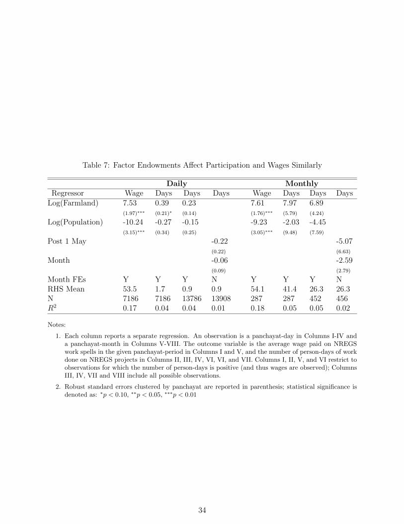
Table 7: Factor Endowments Affect Participation and Wages Similarly

Daily MonthlyRegressor Wage Days Days Days Wage Days Days Days

Log(Farmland) 7.53 0.39 0.23 7.61 7.97 6.89(1.97)∗∗∗ (0.21)∗ (0.14) (1.76)∗∗∗ (5.79) (4.24)

Log(Population) -10.24 -0.27 -0.15 -9.23 -2.03 -4.45(3.15)∗∗∗ (0.34) (0.25) (3.05)∗∗∗ (9.48) (7.59)

Post 1 May -0.22 -5.07(0.22) (6.63)

Month -0.06 -2.59(0.09) (2.79)

Month FEs Y Y Y N Y Y Y NRHS Mean 53.5 1.7 0.9 0.9 54.1 41.4 26.3 26.3N 7186 7186 13786 13908 287 287 452 456R2 0.17 0.04 0.04 0.01 0.18 0.05 0.05 0.02

Notes:

1. Each column reports a separate regression. An observation is a panchayat-day in Columns I-IV anda panchayat-month in Columns V-VIII. The outcome variable is the average wage paid on NREGSwork spells in the given panchayat-period in Columns I and V, and the number of person-days of workdone on NREGS projects in Columns II, III, IV, VI, VI, and VII. Columns I, II, V, and VI restrict toobservations for which the number of person-days is positive (and thus wages are observed); ColumnsIII, IV, VII and VIII include all possible observations.

2. Robust standard errors clustered by panchayat are reported in parenthesis; statistical significance isdenoted as: ∗p < 0.10, ∗∗p < 0.05, ∗∗∗p < 0.01

34

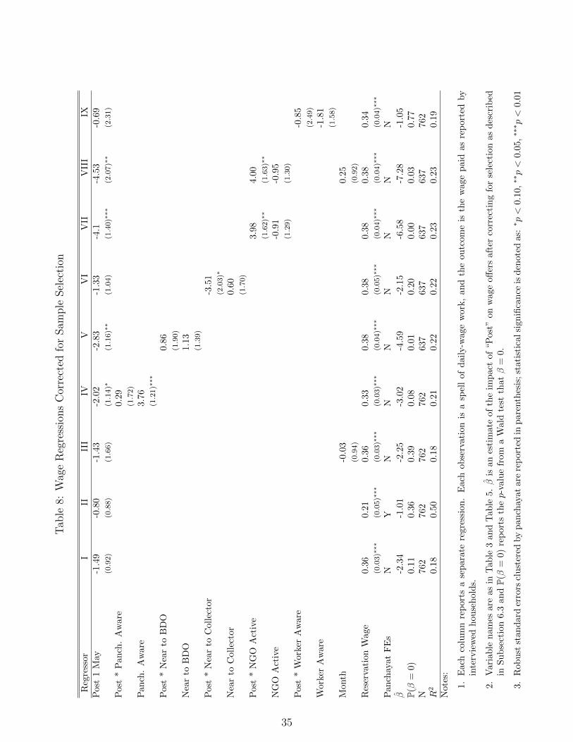
Tab

le8:

Wag

eR

egre

ssio

ns

Cor

rect

edfo

rSam

ple

Sel

ecti

on

Reg

ress

orI

IIII

IIV

VV

IV

IIV

III

IXP

ost

1M

ay-1

.49

-0.8

0-1

.43

-2.0

2-2

.83

-1.3

3-4

.1-4

.53

-0.6

9(0.92)

(0.88)

(1.66)

(1.14)∗

(1.16)∗

∗(1.04)

(1.40)∗

∗∗(2.07)∗

∗(2.31)

Pos

t*

Pan

ch.

Aw

are

0.2

9(1.72)

Pan

ch.

Aw

are

3.7

6(1.21)∗

∗∗

Pos

t*

Nea

rto

BD

O0.8

6(1.90)

Nea

rto

BD

O1.1

3(1.39)

Pos

t*

Nea

rto

Col

lect

or-3

.51

(2.03)∗

Nea

rto

Col

lect

or0.6

0(1.70)

Pos

t*

NG

OA

ctiv

e3.9

84.0

0(1.62)∗

∗(1.63)∗

∗

NG

OA

ctiv

e-0

.91

-0.9

5(1.29)

(1.30)

Pos

t*

Wor

ker

Aw

are

-0.8

5(2.49)

Wor

ker

Aw

are

-1.8

1(1.58)

Mon

th-0

.03

0.2

5(0.94)

(0.92)

Res

erva

tion

Wag

e0.

360.

210.3

60.3

30.3

80.3

80.3

80.3

80.3

4(0.03)∗

∗∗(0.05)∗

∗∗(0.03)∗

∗∗(0.03)∗

∗∗(0.04)∗

∗∗(0.05)∗

∗∗(0.04)∗

∗∗(0.04)∗

∗∗(0.04)∗

∗∗

Pan

chay

atF

Es

NY

NN

NN

NN

N

β̂-2

.34

-1.0

1-2

.25

-3.0

2-4

.59

-2.1

5-6

.58

-7.2

8-1

.05

P(β

=0)

0.11

0.36

0.3

90.0

80.0

10.2

00.0

00.0

30.7

7N

762

762

762

762

637

637

637

637

762

R2

0.18

0.50

0.1

80.2

10.2

20.2

20.2

30.2

30.1

9N

otes

:

1.E

ach

colu

mn

rep

orts

ase

par

ate

regr

essi

on.

Eac

hob

serv

ati

on

isa

spel

lof

dail

y-w

age

work

,an

dth

eou

tcom

eis

the

wage

paid

as

rep

ort

edby

inte

rvie

wed

hou

seh

old

s.

2.V

aria

ble

nam

esar

eas

inT

able

3an

dT

able

5.β̂

isan

esti

mate

of

the

imp

act

of

“P

ost

”on

wage

off

ers

aft

erco

rrec

tin

gfo

rse

lect

ion

as

des

crib

edin

Su

bse

ctio

n6.

3an

dP(β

=0)

rep

orts

thep-v

alu

efr

om

aW

ald

test

thatβ

=0.

3.R

obu

stst

and

ard

erro

rscl

ust

ered

by

pan

chay

atar

ere

port

edin

pare

nth

esis

;st

ati

stic

alsi

gn

ifica

nce

isd

enote

das:∗ p<

0.10,∗∗p<

0.05,∗∗∗ p<

0.01

35

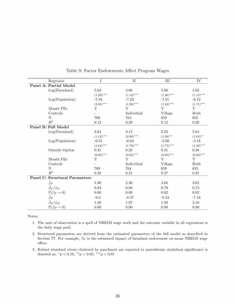
Table 9: Factor Endowments Affect Program Wages

Regressor I II III IVPanel A: Partial Model

Log(Farmland) 5.63 4.68 5.06 4.02(1.29)∗∗∗ (1.12)∗∗∗ (1.36)∗∗∗ (1.15)∗∗∗

Log(Population) -7.84 -7.23 -7.01 -6.12(2.05)∗∗∗ (1.90)∗∗∗ (1.93)∗∗∗ (1.71)∗∗∗

Month FEs Y Y Y YControls - Individual Village BothN 769 764 659 655R2 0.12 0.20 0.12 0.20

Panel B: Full ModelLog(Farmland) 3.64 3.15 3.22 2.64

(1.12)∗∗∗ (0.99)∗∗∗ (1.26)∗∗ (1.05)∗∗

Log(Population) -6.31 -6.04 -5.68 -5.18(1.84)∗∗∗ (1.79)∗∗∗ (1.75)∗∗∗ (1.59)∗∗∗

Outside Option 0.31 0.28 0.31 0.28(0.03)∗∗∗ (0.03)∗∗∗ (0.03)∗∗∗ (0.04)∗∗∗

Month FEs Y Y Y YControls - Individual Village BothN 769 764 659 655R2 0.28 0.31 0.27 0.31

Panel C: Structural Parameters

β̂F 5.30 4.36 4.68 3.65

β̂F /α̂F 0.83 0.80 0.79 0.73P(βF = 0) 0.00 0.00 0.02 0.02

β̂P -9.2 -8.37 -8.24 -7.16

β̂P /α̂P 1.89 1.97 1.92 2.10P(βP = 0) 0.00 0.00 0.00 0.00

Notes:

1. The unit of observation is a spell of NREGS wage work and the outcome variable in all regressions isthe daily wage paid.

2. Structural parameters are derived from the estimated parameters of the full model as described inSection ??. For example, β̂F is the estimated impact of farmland endowment on mean NREGS wageoffers.

3. Robust standard errors clustered by panchayat are reported in parenthesis; statistical significance isdenoted as: ∗p < 0.10, ∗∗p < 0.05, ∗∗∗p < 0.01

36