Marieke Jesse and Maite SeverinsTheoretical EpidemiologyFaculty of Veterinary ScienceUtrecht

Mathematical Epidemiology of infectious diseases

Chapter 1Section 1.1 until 1.3.3

Consider a virgin closed population and assume that at least one disease-causing organism is introduced in at least one host.

Then the following questions arise:

• Does this cause an epidemic?

• If so, with what rate does the number of infected hosts increase during the rise of the epidemic?

• What proportion of the population will ultimately have experienced infection?

1.2 Initial growth

1.2.1 Initial growth on a generation basis

R0 (the basis reproduction ratio):The expected number of secondary cases per primary case in a ‘virgin’ population

This ratio is a threshold parameter; in the sense of an epidemic, if

R0 < 1 : the number of infected decreases and the disease dies out R0 > 1 : an epidemic can occur.

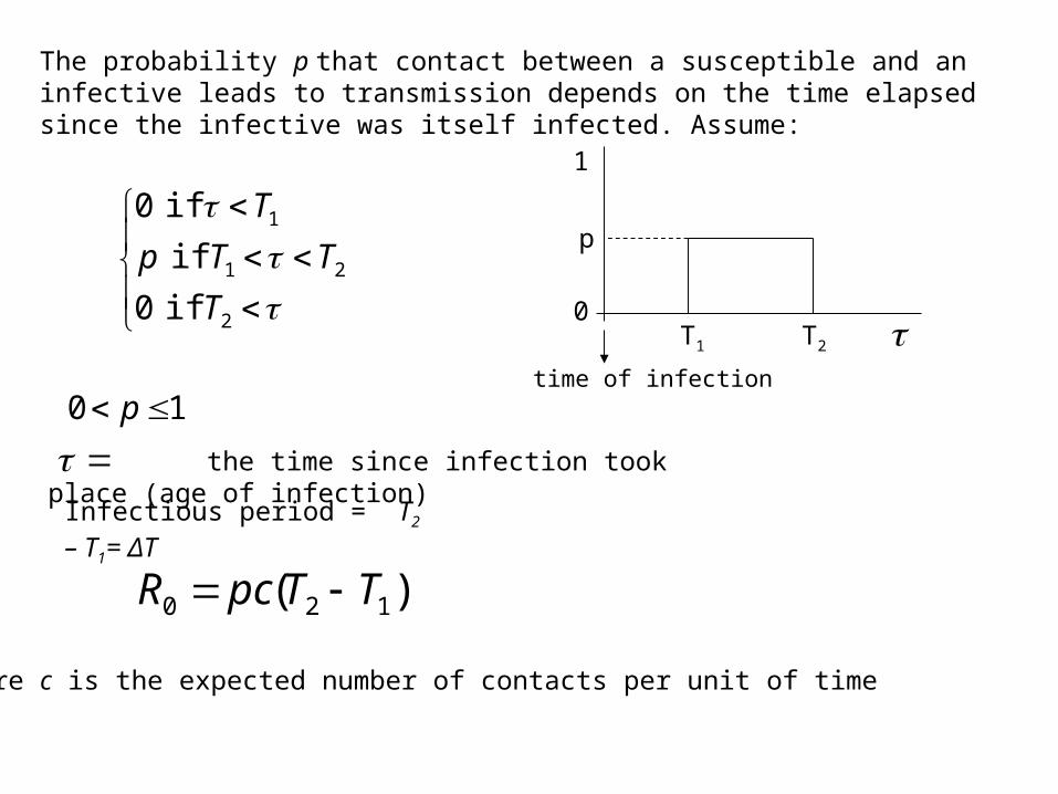
The probability p that contact between a susceptible and an infective leads to transmission depends on the time elapsed since the infective was itself infected. Assume:

2

21

1

if 0

if

if 0

T

TTp

T

the time since infection took place (age of infection)

10 p

Infectious period = T2 – T1= ΔT

)( 120 TTpcR

where c is the expected number of contacts per unit of time

p

T1 T2

0

1

time of infection

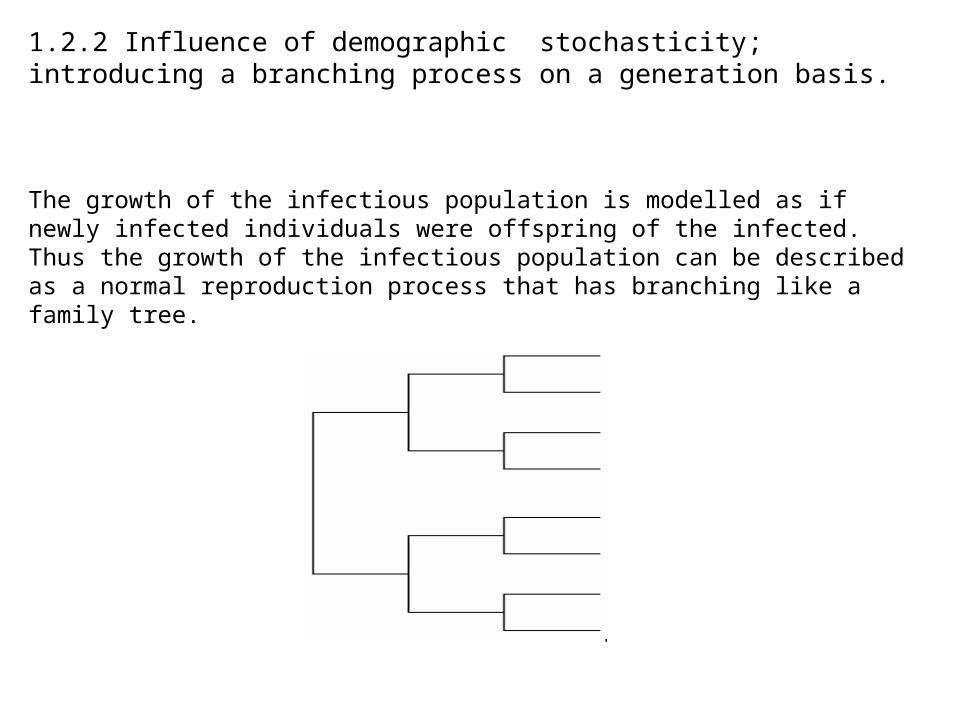
1.2.2 Influence of demographic stochasticity; introducing a branching process on a generation basis.

The growth of the infectious population is modelled as if newly infected individuals were offspring of the infected. Thus the growth of the infectious population can be described as a normal reproduction process that has branching like a family tree.

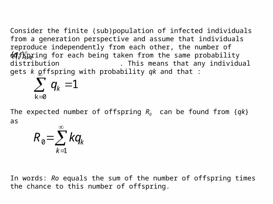
Consider the finite (sub)population of infected individuals from a generation perspective and assume that individuals reproduce independently from each other, the number of offspring for each being taken from the same probability distribution . This means that any individual gets k offspring with probability qk and that :

0}{ kkq

1 0k

kq

The expected number of offspring R0 can be found from {qk} as

In words: Ro equals the sum of the number of offspring times the chance to this number of offspring.

1

0k

kkqR

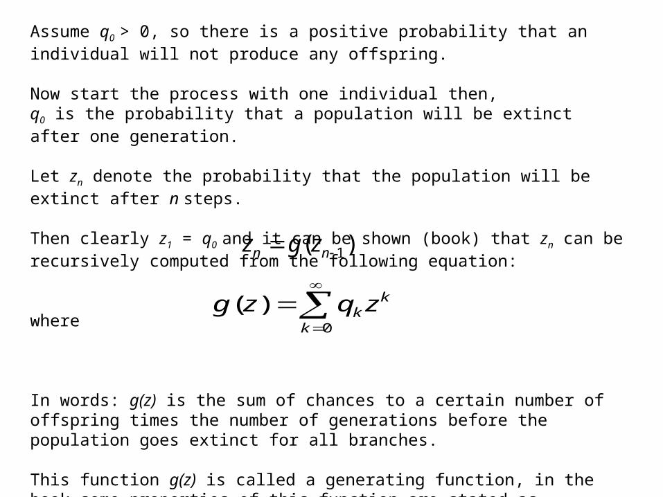
Assume q0 > 0, so there is a positive probability that an individual will not produce any offspring.

Now start the process with one individual then,q0 is the probability that a population will be extinct after one generation.

Let zn denote the probability that the population will be extinct after n steps.

Then clearly z1 = q0 and it can be shown (book) that zn can be recursively computed from the following equation:

where

In words: g(z) is the sum of chances to a certain number of offspring times the number of generations before the population goes extinct for all branches.

This function g(z) is called a generating function, in the book some properties of this function are stated as exercise 1.5.

0

)(k

kk zqzg

)( 1 nn zgz

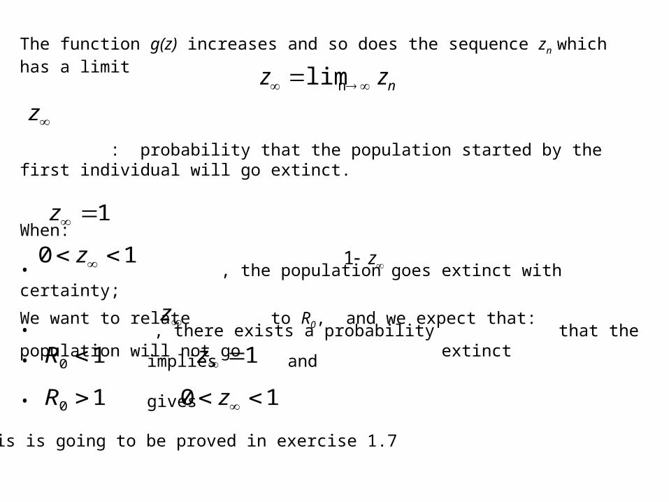
The function g(z) increases and so does the sequence zn which has a limit

: probability that the population started by the first individual will go extinct.

When:

• , the population goes extinct with certainty;

• , there exists a probability that the population will not go extinct

We want to relate to R0, and we expect that:

• implies and

• gives

nzz limn

z

z1

1z

10 z

10 R 1z

10 z10 R

This is going to be proved in exercise 1.7

z

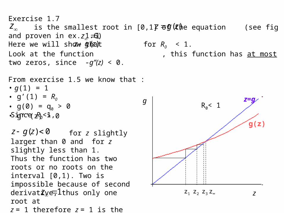
Exercise 1.7 is the smallest root in [0,1] of the equation (see fig and proven in ex. 1.6)Here we will show that for R0 < 1. Look at the function , this function has at most two zeros, since -g’’(z) < 0.

From exercise 1.5 we know that :• g(1) = 1 • g’(1) = R0

• g(0) = q0 > 0• g’’(z) > 0

1z)(zgz

Since R0<1,

for z slightly larger than 0 and for z slightly less than 1. Thus the function has two roots or no roots on the interval [0,1). Two is impossible because of second derivative, thus only one root atz = 1 therefore z = 1 is the smallest root and for R0< 1.

0)( zgz

z )(zgz

z

g z=g

g(z)

R0< 1

z1 z2 z3 z∞1z

Conclusion:

Even in the situation where the infective agent has the potential of exponential growth, i.e. R0 > 1, it still may go extinct due to an unlucky (for the parasite) combination of events while numbers are low. The probability that such an extinction happens, when we start out with exactly one primary case, can be computed as a specific root of the equation )(zgz

The probability that the introduction of an infected host from outside does not lead to an epidemic can be expressed in terms of the parameters. Therefore function g (or, equivalently, the probabilities qk) has to be derived.

The probabilities depends on the used probability distrubtions, e.g. Poisson or binomial.

It is important to notice that although the basic reproduction number R0 remains the same, the probability depends on the function g(z).

Conclusion: different kinds of transmission models yields different values for though the basis reproduction number Ro remains the same.

z

z

z

1.2.3 Initial growth in real time

So far we have looked at initial growth on a generation basis and found a threshold occurring by a parameter R0 and that for R0 above this threshold, there exists a positive probability that introduction of one primary case does not lead to explosive exponential growth.

For simple models the values for R0 and can be determined explicitly in terms of the parameters of the model. However, measuring growth on a generation basis is not possible in real life because it does not correspond to our observations, where the infection generations overlap.

z

z

What is observed during the initial phase of a real epidemic is exponential growth as follows:

for some growth rate r > 0, constant C > 0 were,I(t), is the prevalence, the number of cases notified up to time t,

rtCetI )(

2

1

)()(T

Tdtipcti

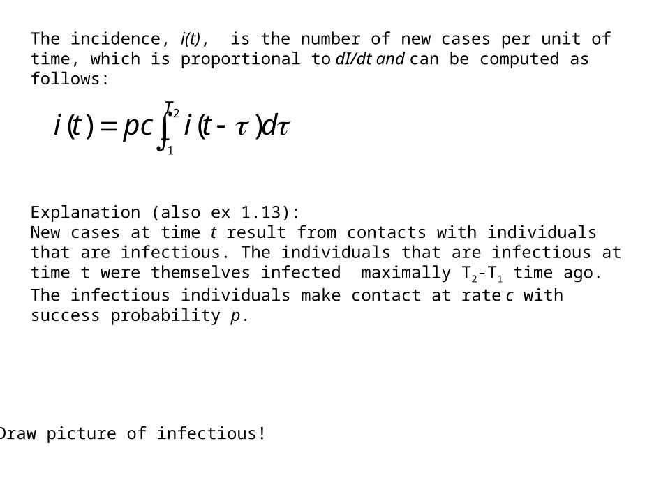
The incidence, i(t), is the number of new cases per unit of time, which is proportional to dI/dt and can be computed as follows:

Explanation (also ex 1.13):New cases at time t result from contacts with individuals that are infectious. The individuals that are infectious at time t were themselves infected maximally T2-T1 time ago. The infectious individuals make contact at rate c with success probability p.

Draw picture of infectious!

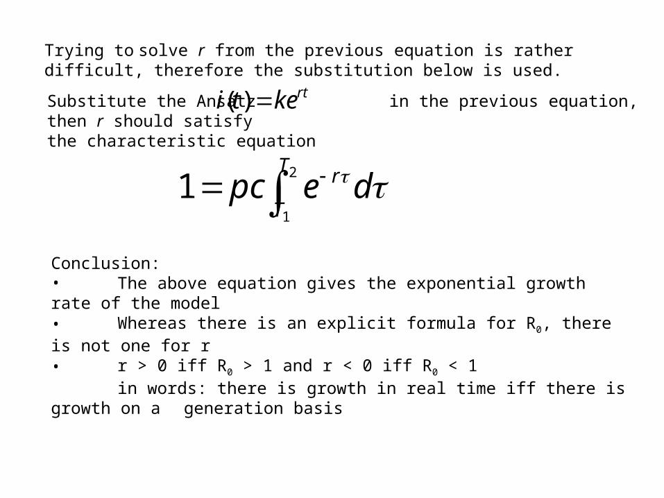
Substitute the Ansatz in the previous equation, then r should satisfythe characteristic equation

rtketi )(

2

1

1T

T

r depc

Conclusion:• The above equation gives the exponential growth rate of the model• Whereas there is an explicit formula for R0, there is not one for r• r > 0 iff R0 > 1 and r < 0 iff R0 < 1

in words: there is growth in real time iff there is growth on a generation basis

Trying to solve r from the previous equation is rather difficult, therefore the substitution below is used.

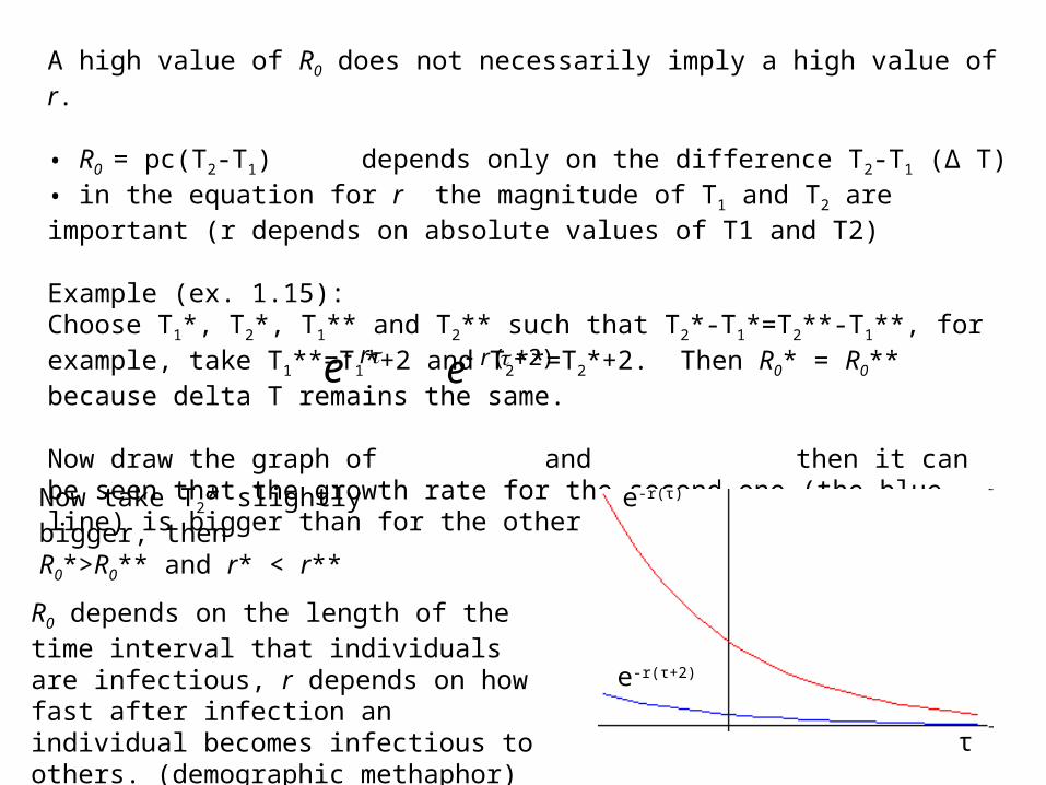
A high value of R0 does not necessarily imply a high value of r.

• R0 = pc(T2-T1) depends only on the difference T2-T1 (Δ T)• in the equation for r the magnitude of T1 and T2 are important (r depends on absolute values of T1 and T2)

Example (ex. 1.15):Choose T1*, T2*, T1** and T2** such that T2*-T1*=T2**-T1**, for example, take T1**=T1*+2 and T2**=T2*+2. Then R0* = R0** because delta T remains the same.

Now draw the graph of and then it can be seen that the growth rate for the second one (the blue line) is bigger than for the other one, so r* < r**

re )2( re

Now take T2* slightly bigger, thenR0*>R0** and r* < r**

R0 depends on the length of the time interval that individuals are infectious, r depends on how fast after infection an individual becomes infectious to others. (demographic methaphor)

e-r(τ)

e-r(τ+2)

τ

Now we have answered two of our questions initially asked:

• Does this cause an epidemic?

• If so, with what rate does the number of infected hosts increase during the rise of the epidemic?

One question still remains:

What proportion of the population will ultimately have experienced infection?

1.3. The final size

1.3.1 The standard final-size equation

In a closed population and with infection leading to either immunity or death, the number of susceptibles decreases and must therefore have a limit.

• Will the number of susceptible be zero at infinity? or • Will some fraction of the population never get infected?

)1)(()(ln 0 sRs

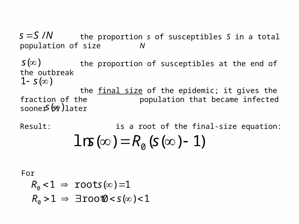
the proportion s of susceptibles S in a total population of size N

the proportion of susceptibles at the end of the outbreak

the final size of the epidemic; it gives the fraction of the population that became infected sooner or later

Result: is a root of the final-size equation:

)(1 s

)(s

NSs /

)(s

For

1)(root 10 sR

1)( 0root 10 sR

Conclusion:

• a certain fraction escapes from ever getting the disease

• this fraction is completely determined by R0

• the larger R0 is, the smaller the fraction

)(s

)(s

)(s

1.3.2 Derivation of the final-size equation

Ex. 1.21

S the size of the subpopulation of susceptiblesI the size of the subpopulation of infectivesR the size of the subpopulation of removed

Force of infection the probability per unit of time for a susceptible to become infected, this is proportional to I

tranmission rate (the constant of proportionality of the force of infection)

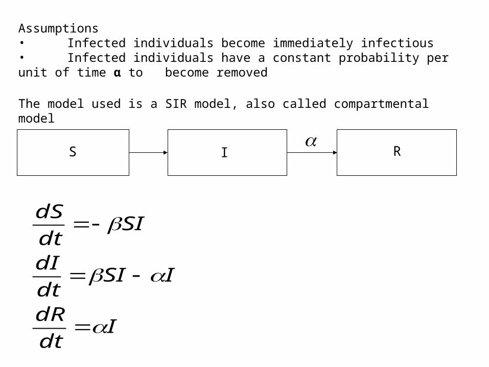
Assumptions• Infected individuals become immediately infectious• Infected individuals have a constant probability per unit of time α to become removed

The model used is a SIR model, also called compartmental model

Idt

dR

ISIdt

dI

SIdt

dS

S I R

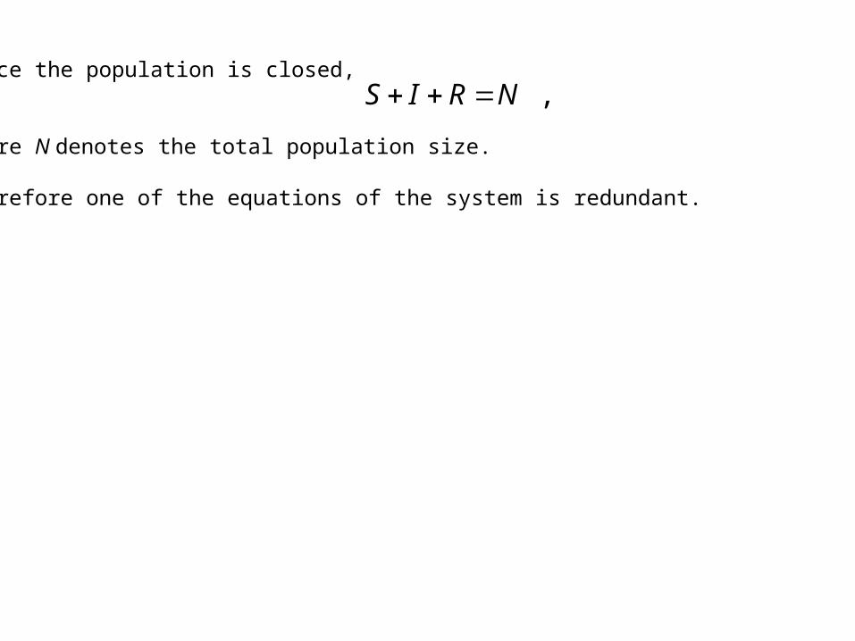
Since the population is closed,

where N denotes the total population size.

Therefore one of the equations of the system is redundant.

, NRIS

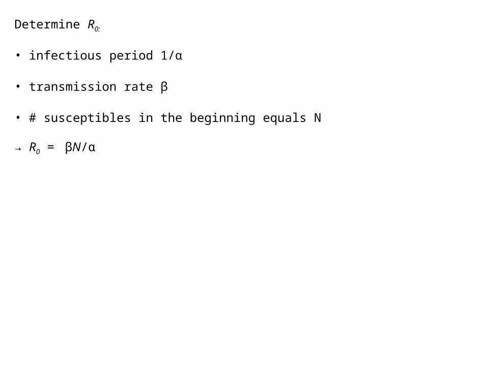
Determine R0:

• infectious period 1/α

• transmission rate β

• # susceptibles in the beginning equals N

→ R0 = βN/α

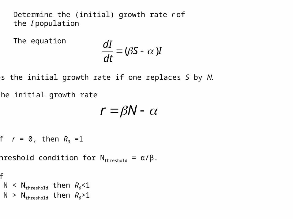
Determine the (initial) growth rate r of the I population

The equation

ISdt

dI)(

gives the initial growth rate if one replaces S by N.

So the initial growth rate

Nr

If r = 0, then R0 =1

Threshold condition for Nthreshold = α/β.

If • N < Nthreshold then R0<1• N > Nthreshold then R0>1

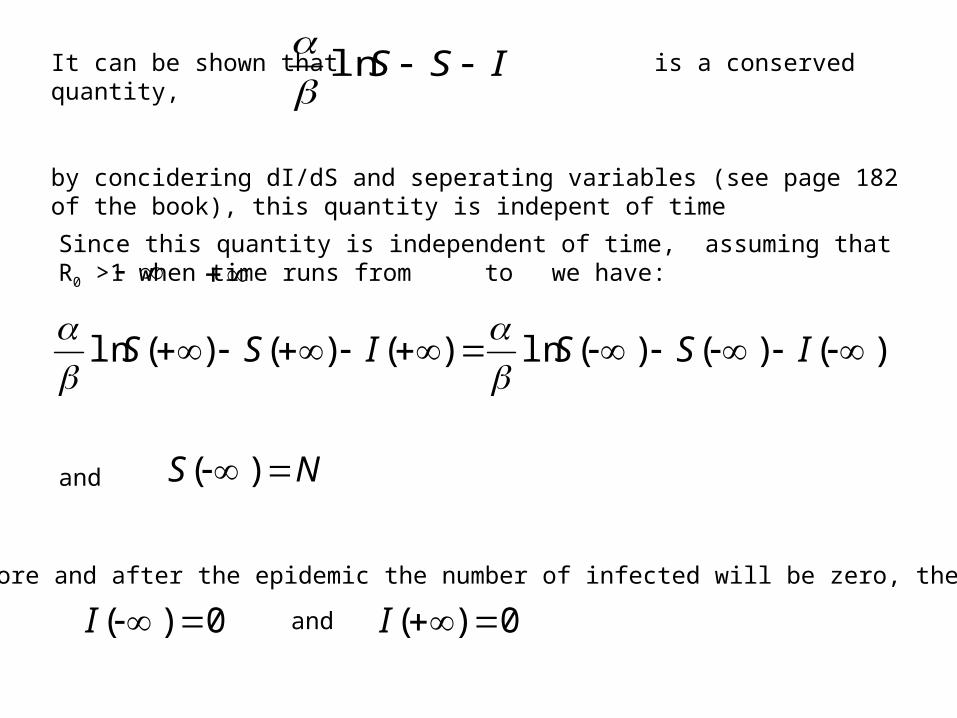
It can be shown that is a conserved quantity,

by concidering dI/dS and seperating variables (see page 182 of the book), this quantity is indepent of time

ISS ln

Since this quantity is independent of time, assuming that R0 >1 when time runs from to we have:

and

)()()(ln)()()(ln ISSISS

NS )(

0)( I

Both before and after the epidemic the number of infected will be zero, therefore:

and0)( I

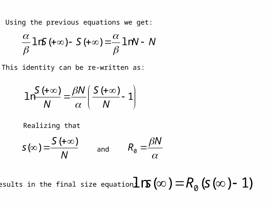
NNSS ln)()(ln

Using the previous equations we get:

This identity can be re-written as:

1

)()(ln

N

SN

N

S

Realizing that

N

Ss

)()(

and

N

R 0

Results in the final size equation: )1)(()(ln 0 sRs

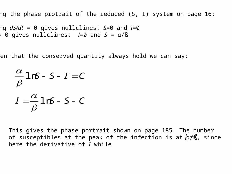
Drawing the phase protrait of the reduced (S, I) system on page 16:

setting dS/dt = 0 gives nullclines: S=0 and I=0dI/dt = 0 gives nullclines: I=0 and S = α/ß

CSSI

CISS

ln

ln

Given that the conserved quantity always hold we can say:

This gives the phase portrait shown on page 185. The number of susceptibles at the peak of the infection is at α/ß, since here the derivative of I while 0I

Overshoot phenomenon:

The root, , of the final size equation becomes smaller when N increases.Why does the fráction of susceptibles at the end of the epidemic become smaller with increasing population size? This is due to the overshoot-phenomenon:

When an epidemic starts with a larger number of susceptibles, the number of infected at the peak of the epidemic will be very large. Large enough to infect a huge number of susceptibles even though the epidemic is decreasing.

)(s

In exercise 1.21 (viii) The SIR model of page 15 is reformulated in terms of fractions of individuals. It is important to pay attention to the dimensions of the parameters and to think carefully about the new interpretation of them

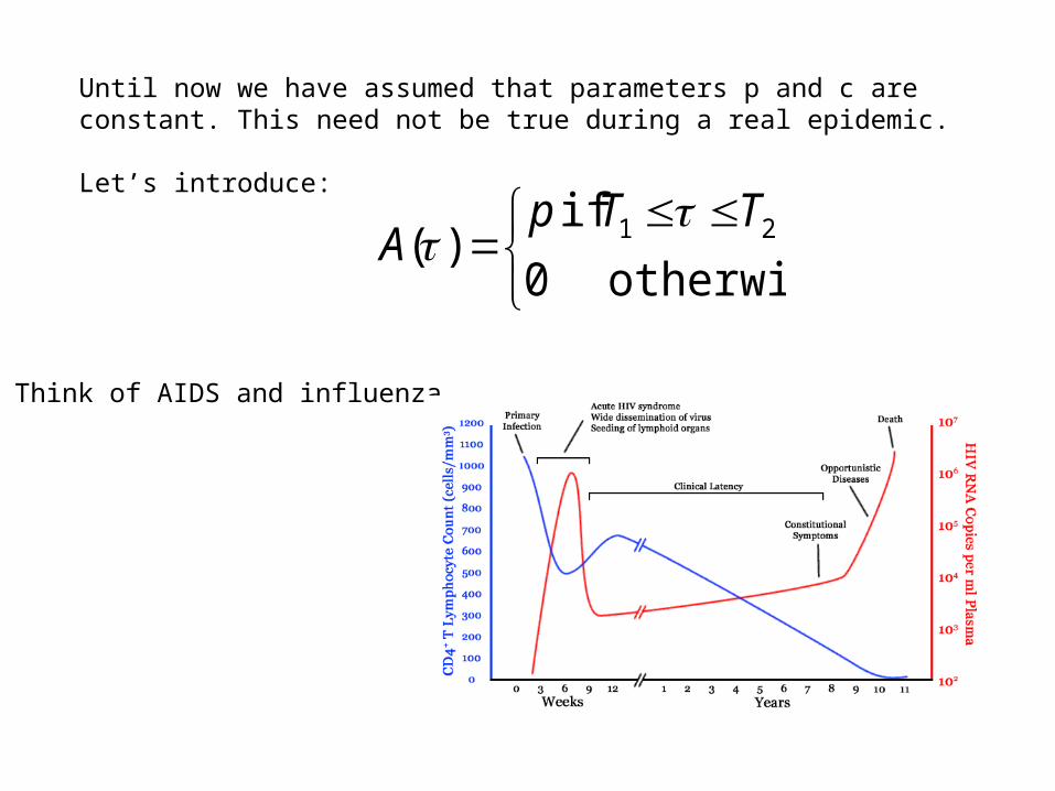
Until now we have assumed that parameters p and c are constant. This need not be true during a real epidemic.

Let’s introduce:

otherwise 0

if )( 21 TTp

A

Think of AIDS and influenza

In the last part of section 1.3.2, also assumptions regarding the contact rate (c) are made more explicit and related to the validity of the final size equation.

Until now we have assumed that the contact rate is a constant. Does the final size equation still hold when this is not the case, for example when the contact rate is proportional to the population density?

It is shown that the final size equation hold when the disease doesn’t cause any death, i.e that it interferes in no way with the contact process. Or if, the disease has a high mortality, the final size equation hold when the contact intensity is proportional to the population density.