Intergovernmental Oceanographic Commission technical series

21

Bruun memorial lectures, 197g Presented at the eleventh session of the IOC Assembly, Unesco, Paris, I November 1979

Marine environment and ocean resources

Unesco, I980

The designations employed and the presentation of the material in this publication do not imply the expression of any opinion whatsoever on the part of the Secretariats of Unesco and IOC concerning the legal status of any country or territory, or of its authorities, or concerning the delimitations of the frontiers of any country or territory.

ISBN 92-3-101947-3 Ftench edition 92-3-201947-7 Spanish edition 92-3-301947-0 Russian edition 92-34019474 Published in 1981 by the United Nations Educational, Scientific and cultural Organization, 7, place de Fontenoy ,75 700 Paris Composed and printed in Unesco’s wodcshops

6 Unesco 1981 Printed in France

Preface

Presented during the eleventh session of the Assembly of the Intergovernmental Oceanographic Commission, this series of lectures is dedicated to the memory of the noted Danish oceanographer and first chairman of the Comrnis- sion, Dr. Anton Frederick Bruun. The "Bruun Memorial Lectures" were established in accordance with IOC reso- lution VI-19 in which the Commission proposed that im- portant inter-sessional developments be summarized by speakers in the fields of solid earth studies; physical and chemical oceanography and meteorology; and marine bio- logy. The Commission further requested Unesco to arrange for publication of the lectures and it was subsequently decided to include them in the "IOCTechnical Series".

Anton Bruun was born on 14 December 1901, the first son of a farmer; however, a severe attack of polio in his childhood led him to follow an academic, rather than an agrarian, career.

In 1926 Bruun received a Ph.D. in zoology, having several years earlier already started working for the Danish Fishery Research Institute. This association took him on cruises in the North Atlantic where he learned from such distinguished scientists as Johannes Schmidt, C.G. Johannes Petersen and Th. Mortensen. Of even more importance to his later activities was his

participation in the Dana Expedition's circumnavigation of the world in 1928-1930, during which time he acquired further knowledge of animal life of thesea,general oceano- graphy and techniques in oceanic research.

In the following years Bruun devoted most of his time to studies of animals from the rich Dana collections and to the publication of his treatise o n the flying fishes of the Atlantic. In 1938 he was named curator at the Zoo- logical Museum of the University of Copenhagen and later also acted as lecturer in oceanology.

From 1945 to 1946 he was the leader of the Atlantide Expedition to the shelf areas of West Africa. This was fol- lowed by his eminent leadership of the Galathea Expedi- tion in 1850-1952, which concentrated on the benthic fauna below 3,000 m. and undertook the first exploration of the deepsea trenches, revealing a special fauna to which he gave the n a m e "hadal".

The last decade of Bruun's life was devoted to inter- national oceanography. H e was actively involved in the establishment of bodies such as thescientific Committee on Oceanic Research (SCOR), the International Advisory Committee on Marine Sciences (IACOMS), the Inter- national Association for Biological Oceanography (IABO) and the Intergovernmental Oceanographic Commission (IOC); he was elected first Chairman of the Commission in 1961.

His untimely death a few months later, on 13 December 1961, put an end to many hopes and aspirations, but Anton Bruun will be remembered for his inspiring influence on fellow oceanographers and his scientific contribution to the knowledge of the sea which he loved so much.

3

Table of contents

OPENING STATEMENT Dr. Neil J. Campbell, (First Vice-chairman) ......... ............ 5 ..........

NON-LIVI NG MAR IN E RESOURCES Prof. Dr. Eugen Seibold .................................................... 7

OCEAN ENERGY Dr. Kenzo Takano. ....................................................... 15

SHORT-TERM CLIMATIC CHANGE: A PHYSICAL OCEANOGRAPHER’S POINT OF VIEW Dr. J.S. Godfrey ......................................................... 21

PRODUCTION IN THE CENTRAL GYRES OF THE PACIFIC Dr. D.H. Cushing.. ....................................................... 31

4

Opening statement Dr. Neil J. Campbell, First Vice-chairman

Ladies and Gentlemen, It is m y honour to welcome you to the Bruun Memorial Lectures on the occasion of the Xlth Assembly of the Intergovernmental Oceanographic Commission. This set of four lectures which you will hear today is one of a series of scientific sessionscommemorating the name of Dr.Anton Bruun w h o was an eminent marine biologist not only in his native country of Denmark, but also throughout the world. During his outstanding career; he made numerous significant contributions to marine biology and deep ocean benthic fauna research. H e was a m a n devoted to research, to teaching, and to the overall advancement of the marine sciences. In addition, Anton Bruun was one of the leading figures of his day in establishing the Intergovernmental Oceanographic Commission and was elected its first Chair- m a n in 1961. With his untimely death in only his first year of office, this Commission as well as the oceanographic community in general suffered a great loss. It was for this reason that the Commission decided to honour his name through the dedication of a series of lectures at each Assembly .

A title of our session today is: The Marine Environment and Ocean Resources. Increasingly, the world is looking towards the oceans as a source of food, raw materials and energy. This is particularly true of developing countries some of which, unfortunately, have not been blessed with climates conducive to agricultural production or land- based geological formations conducive to mineral exploita- tion. And, of course, developed and developing countries alike face the grim prospect of dwindling conventional sources of energy.

W e are indeed fortunate therefore, in having with us today four very distinguished scientists w h o can speak with authority on what the oceans hold for the future. In order of presentation, Dr. Eugen Seibold of the Federal Republic of Germany will speak on the subject of non-

renewable resources; Dr. Kenzo Takano will address the subject of ocean energy; Dr. David Rochford of Australia will present a paper on ocean climate; and Dr. David Cushing of the United Kingdom will present a paper on living resources. In the spirit of co-operation upon which the IOC was founded, Dr. Rochford’s contribution will be on behalf of his Australian colleague Dr. Stuart Godfrey who, having prepared the paper is, owing to illness, unable to be amongst us today.

The eleventh session of the IOC Assembly has passed resolutions which will bring the fcw topics about to be discussed into the mainstream of IOC activities. T h e Anton Bruun lectures today, therefore, could hardly be more timely.

Before our distinguished speakers start their lectures, I wish to thank them on behalf of the IOC and on m y o w n behalf for their valuable participation, which I a m sure will be greatly appreciated by the Assembly.

As I mentioned before, our first guest speaker is Prof Dr. Eugen Seibold, Federal Republic of Germany, the Director of the Geological Institute of the University of Kiel. H e studied geological sciences at the University of Tubingen and University of Bonn and obtained his doc- torate in 1948 specializing in sedimentology. H e hastaught at the Geological Institute, University of Tubingen, the Qeological Institute of the Technical University Karlsruhe as well as at the University of Kiel. His research interests are tectonics, sedimentology, and applied marine geology. In his studies, he has worked extensively in the Baltic, the North Sea, the East Atlantic, the Indian Ocean and the Persian Gulf, serving on numerous occasions as the Chief Scientist of the R.V. Meteor and R.V. Valdivia. H e parti- cipated as Cochief scientist on the Elmar Challenger Leg 41 off the West Coast of Africa and aboard the Sonne off north west Australia.

M a y I present Dr. Eugen Seibold.

5

Non-living marine resources Professor Dr. Eugen Seibold,

Geological- Palaeon tological Institute, Kiel University, Federal Republic of Germany

Ladies and Gentlemen, Speaking to you today presents m e with the welcome opportunity to thankthe Intergovernmental Oceanographic Commission (IOC) and you as its responsible group for the interest and help which I as a scientist, along with many of m y colleagues, have received since the Inter- national Indian Ocean Expedition (IIOE). It is indeed a pleasure and an honour to address you today in memory of Anton Frederick Bruun, m y former scientific neighbour in Denmark.

T h e assembly is composed of officials of high rank in the administrations of their respective countries-diplomats, naval officers, engineers and marine scientists. F e w of you m a y be geologists like myself, and I personally feel c o m - petent to speak only about marine geology. Therefore I shall exclude resources from seawater.

During the lecture I shall try: (1 ) to show this topic as an example of the necessity of

international co-operation. A s a geologist I must add that up to now, IOC has been rather hesitant in promoting geoscience projects compared, for example, with other United Nations programmes under which the Committee for Co-ordination of Joint Prospecting for Mineral Resources in the South Pacific Offshore Areas (CCOP/ S O P A C ) is sponsored. Nevertheless, with the help of IOC: - excellent global scenarios were given in workshops as in

Ponza (1969). in Hawaii (19711,and in Mauritius (1976). Parts of these ideas were included in the Long-term and Expanded Programme of Oceanic Research (LEPOR);

- important results were, and will continue to be, achieved by some 12 (out of 61) Scientific Committee on Oceanic Research ( S C O R ) working groups related to our topic;

- effective work was done in editing the General Bathy- metric Chart of the Ocean (GEBC0)-of which about 40% of the sheets have been published-and the Geolo- gical/Geophysical Atlas of the International Indian Ocean Expedition. Finally, the Conimission of Marine Geology of ICSU

and the International Geological Correlation Programme are actively building bridges between scientists, countries and disciplines.

(2) To present something for the diplomats among you. Diplomats are particularly interested in learning the essen- tials and, on the other hand, in being aware of the newest developments.

(3) To take the engineers among you, at least vicariously, o n board ship to show you some n e w methods.

(4) To discuss something of the relationships between basic and applied research, for the top decision-makers among you. This is not only because I k n o w that without the money which you make available no research would be possible, but also because it is your responsibility to see that the knowledge gained is correctly used.

(5) Finally, to c o m e to naval officers and take from their many virtues only one: punctuality, something a professor frequently forgets in his enthusiasm in lecturing.

Challenges and Concepts

For millenia m a n has fished in the sea and obtained mussels, sand and salt near beaches. Only for a century has he known something about the deep sea bottom. Only for half a century has he produced offshore oil. Our know- ledge of the morphology of ocean bottoms is no better than our knowledge of continents two centuries ago; that is to say, basically, it is restricted to coastal zones and some traverses of expeditions into the vast oceanic areas. A s an example, hardly any published data existed for water depths in the area 80" - 90" E and 40" - 50" S when w e prepared the IIOE-Atlas in Moscow. That is to say, little was known of an area of 860,000 km 2 , or roughly the surface area of France and Italy together. IOC was asked to prepare, together with the International Hydro- graphic Organization (IHO), a m a p 1:lO or 1:6 million by M a y 1982 for the Third United Nations L a w of the Sea Conference (UNCLOS) which it is hoped will have no substantial blank spots.

Even less is known of the character of sediments or structures under the sea floor. Therefore the first task for a marine geologist is to fill some of these huge gaps. With regard to m y lecture about marine mineral resources, I a m therefore very much in doubt as to whether some of the published estimates of the magnitude of these resources from the seabed are really useful. Existing guesses, often too optimistic, m a y even make political agreement more difficult in the UNCLOS debates.

How does one find marine mineral resoyces? Econo- mically important depositsare almost always concentrated in small areas, because many factors must have combined favourably to produce an area of enrichment, A s some of you know, it is usually easier to find a mine by chance than to predict one-as to fall in love is easier than io predict an engagement. Nevertheless the immensity Df the oceanic' areas involved and :he very high costs of re. search therein are strong argummts for a strategy: a con- cept for prospecting the sea floor, at least te predict areas without any chance of economic mineral concentrations.

During the last two decades marine geophysicists and geologists have developed such a strategy known as the concept of ocean floor spreading and plate tectonics, and Arthur E. Maxwell presented part of these concepts during a Bruun Memorial lecture in 1969. Y o u will remem- ber from his lecture that these theories of the evolution of the oceans are as revolutionary today as the ideas of Charles Darwin were a century ago. S o m e remarks for the diplomats interested in essentials will follow.

A n increased heat flow from the mantle of the earth, combined with cracks and faults, produced and still pro- duces updoming of the earth's crust beneath the con- tinents and the oceans (Fig. la). Hot mantle material penetrates to the surface, forming basaltic lava, dikes and sills (Fig. Ib). Both sides of these weak linear zones are drifting apart from the "spreading centre". Veloci-

+ I -

: * I 1 WllHCEYIRAL RIFT

I 1 I I ISLOP€ I I - Fig. 1: Sea floor spreading conmpt (see text for explanation). cc = continental crust, oc = oceanic crust. After Blissenback & Fellerer (1973).

ties of 1 to more than 10 c m per year have been re- corded. A continuous supply of basalt fills the gaps and forms a n e w oceanic crust (Fig. IC). These processes are at present concentrated near the median lines of most of our oceans. The updomings form the mid-oceanic ridges, generally with water depths of about 2-3 k m (Fig. Id).

T h e spreading oceanic crust cools and subsides. There- fore the water depths increase landwards. W h e n they reach about 4.5 km , a critical situation arises for the carbonate particles produced by marine organisms. They are c o m - pletely dissolved in these water depths. Normal mid- oceanic sedimentation rates of some c m per 1000 years are then reduced to some m m per 1000 years. Such very low sedimentation rates favour the growth and the sur- vival of manganese nodules on the ocean floor, which will be discussed later.

At the continental margins, sedimentation rates are higher by one order of magnitude or more because of the material delivered from the continents. Additionally, due to spreading, the ocean floor often becomes older near the continents. Therefore more time is available to accumulate sediments; and as will be discussed later, thick sediments are a prerequisite for oil and gas formation.

Naturally, this summary of the sea floor spreading and plate tectonics concepts is greatly simplified and covers only parts of the evolution of the oceans. For example, the so-called active margins, with convergent plate boun- daries (Fig. 2)-a focal point for the IOC working group WESTPAC, active since February 1979-are excluded here.

Metal concentrations at divergent plate boundaries

O n a global m a p these spreading centres and mid-oceanic ridges are more than 60,000 k m long and are generally indicated by earthquakes and sometimes by volcanism, as in Iceland. They mark the so-called divergent boundaries of rigid plates, some 100 k m thick and consisting of the earth's crust and upper parts of the mantle (Fig. 2).

Fig. 2: Plate tectonics concapt. Divergent plate. boundaries and mid-oceanic ridges (double lined) with metal occurrences (1-9). Convergent boundaries (spikes). J, K, T = oceanic crust formed during Jurassic, Cretaceous or Tertiary. Based on Chase et al. (1975).

I 1 r I 1 1 1 1 1

8

Fig. 3: Complicated bathymetry of Atlantis-ll Deep and sur- rounding deeps in the Central Red Sea. Water depths in metres. Areas covered with the brines are indicated by hatchings. 225-227 = Glomar Challenger sites. Inset shows concentration of depths at the median line of the Red Sea; most of them are named after research vessels. Based on Backer et al. (1975).

In the Red Sea a continuation of the Med-lndic Ridge penetrates a continental mass (Fig. IC), and in s o m e of its central parts, metalliferous muds of potential econo- mic interest occur. They are concentrated in a small area of 6 x 15 k m in more than 2,000 m water depth, the so- called Atlantic-l l-Deep (Fig. 3). They were detected during the last phase of the IlOE and investigated by research vessels and specialists for U.S.A., U.K., France, m y country and others. Both the foreign governments in- volved, Saudi Arabia and Sudan, helped in organizing these investigatioN-a real example of international co- operation. These muds contain up to 65% iron, up to 2% copper and up to 20% zinc, altogether about 30 mil- lion tons of iron, 2.5 million tons of zinc, 0.5 million tons of copper and 9,000 tons of silver, worth about US $4 billion, if calculated on world prices for 1978. Therefore they are of potential economic interest. A fe w months ago the first trials to p u m p these m u d s aboard and to separate the very fine grained ore particles from the useless m u d were successfully accomplished by a drilling vessel. At the same time the German Research Vessel Valdivia investigated possible effects of these operations on the marine environment. W e all k n o w that exploitation and protection must be coupled, and that marine geologists need the co-operation of marine biologists.

How are these metalliferous muds formed? The metals are delivered from rocks beneath the sea floor by hot, hypersaline waters penetrating Tertiary sediments, and probably from basalts originating from sea floor spreading. This word probably m a y have very important and global consequences, because it m a y indicate that similar ore concentrations could also be detected in small areas along the 60,000 k m long mid-oceanic ridges. U p to n o w about a dozen examples of metal enrichments have been reported from the central areas of such ridges, but unfortunately, most of them occur as hard crusts and consist only of manganese and iron hydroxides and oxides. In March 1978, however, the French research submersible CYANA detected a multicoloured sulphide zone o n the East Pacific Ridge at 21" N, 109O W, in about 3,000 m water depth (Fig. 2, arrow). The zone had zinc contents up to 28%. copper 6% and silver 0.05%. certainly delivered from the basalts underneath and by the same so-called hydro- ther m a I processes.

These last exciting results of pure scientific research are of no economic interest at present, but 60,000 k m provide enough space for discoverers of similar needles in a hay- stack. At present the metal concentrations in the so-called manganese nodules are more interesting economically.

9

Manganese nodules

A s mentioned before, these nodules occur in deep sea areas with reduced sedimentation rates, that is to say they normally occur: (1 ) far from land; and (2) in water depths ranging from 4 to 5 km , with bottom waters aggressive to carbonates, therefore possibly related to Antarctic Bottom Water paths. Red clay or siliceous oozes most commonly form the underlying sediments. The Pacific in general shows the greatest abundance of nodules as compared with the Atlantic or Indian oceans, both of which receive large river discharges supplying terrestrial material (Fig. 4).

Therefore much more work has to be done in various fields.

Scientifically: at present w e cannot predict rich nodule fields because w e don't really understand the processes concentrating nodules of different metals.

Technologically: recovery systems such as the airlift method are only at the experimental stage, as demonstrated in 5,000 m water depth in M a y 1978 by Ocean Manage- ment Inc., an international group, in the Pacific. The extractive metallurgy of nodules is a subject of continuing research. In general, one to three decades are required to commercially demonstrate a n e w technological system.

Fig. 4: Occurrence of manganese nodules in the oceans. After Berger (1 974).

In the 1960s optimistic estimates put the total for manganese nodules somewhere between 0.9 and 20 x 10" tons. During the last decade, intensive investigations have reduced our hopes considerably.

Normally the nodules contain about 15-30% manganese, 15% iron, 0.1 -0.5% nickel, 0.3-1 .O% cobalt and 0.1 -0.4% copper. At present however, only nodules with a cutoff grade of not less than about 2% of combined nickel + cobalt + copper are considered to be of economic value. They occur only sporadically in the world ocean, especially in the Eastern Central Pacific around IOo N. Another pre- requisite for economic exploitation reduces economic areas even more. Nodule densities of more than 15 kg wet weight, or 10 kg dry weight nodules per mz are needed. Unfor- tunately, nodules show a high patchiness in distribution and a high variation in metal contents and in sizes, and occur in different types. Additionally, nodule fields must be free of morphological obstacles and underlain by suit- able sediments to allow recovery of the nodules either by a continuous line bucket system, a centrifugal p u m p system, or the airlift concept. Finally, the enormous investments needed for exploration, and for exploitation systems and processing plants require nodule fields of at least 20,000-30,000 k m 2 , roughly the area of Belgium; or even 80,000 km2, the area of Austria, to guarantee a suf- ficient supply for about two decades.

Economically: only much more experience will give us more realistic figures than the estimates mentioned before. From published data, a guess m a y be made about poten- tial metal reserves in the north Pacific high grade nodule area: nickel 40-100 million tons, copper 30-80 million tons, cobalt 9-20 million tons. For nickel the estimated amount corresponds roughly with world reserves on land; for copper it is about 1/10 of land reserves, and for cobalt land reserves are only about 1/4 or 1/8 of the above estimates. Later estimates for this area are 26 mil- lion tons for nickel, 20 million tons for copper, 4 million tons for cobalt (McKelvey, 1979).

Legally: certainly everybody in this hall is familiar with the ongoing discussions of the Third United Nations L a w of the Sea Conference. Manganese nodules with their highly valuable metal contents are practically confined to the "Area" (... "the sea-bed and ocean floor and subsoil thereof beyond the limits of national jurisdiction". ICNT Article 1; see also Articles 139-192), the core of Arvid Pardo's "common heritage of mankind". In Germany, at least, heirs rarely smile and often fight. Therefore they need lawyers. The more complicated the resultant agree- ments are, the less effective; the more emotion or povder oriented, the more unfair. The same holds true for the L a w of the Sea, O n the one hand mining industry needs a guarantee for continuous work to justify investments both

10

in manpower and in finances. Actually five international consortia are actively engaged in the preparation of deep ocean mining. O n the other hand the potential impact of nodule mining o n world mineral markets has to be con- sidered. In spite of the m a n y unknown factors, Levy (1 979) estimates that in 1990,30% of the world consump- tion of nickel, 2% of copper and 58% of cobalt m a y be supplied by sea-bed mining, and in 2000 these figures would rise to 40-60% for nickel, 34% for copper and 70-100% for cobalt. In 1974 27.5% of the world reserves of cobalt on land were concentrated in Zaire, 27.1% in N e w Caledonia, 14.0% in Zambia and 13.6% in Cuba. In 1977 58% of the world production was contributed by Zaire and 8% by Zambia. Consequently the potential impact of nodule mining m a y have a substantial influence on the economic situation of some developing countries. W e therefore need a spirit of partnership to solve these global problems, rather than of mistrust and confrontation. Let us n o w go back to the lawyers and to science and to m y personal experience: the more regimentation and bureaucracy, the poorer the science. This holds true for research conducted on all minerals of the sea, and I would n o w like to add some remarks about other resources.

Other mechanical and chemical concentrates

In shallow water, the mechanical action of waves and cur- rents concentrates sand and gravel, two important building materials which are becoming increasingly more expensive on land. For example in 1971, U.K. obtained about 12% (= 13.5 million tons) of its total consurnption.from off- shore-a typical situation, because offshore mining of sand and gravel is of economic interest only very near large industrial cities.

A n even higher degree of mechanical Sorting is seen in placer deposits of tin, gold, iron minerals, diamonds and minerals containing titanium or zirconium. Australia is the world's number one producer (98% in 1974) or Ti0,-rutile, and of zirconium (70%) from placers. Tin production is concentrated between Thailand and Indonesia (61% of the world production in 1976 came from there, about 1/6 of which came from offshore).

Iron sands are exploited around Japan and N e w Zealand (Fig. 5).

Today w e can observe these concentration processes by waves on beaches and by currents in rivers. They were active on the shelves when the sea-level was about 100 m lower some 18,000 years ago. Beaches and their placers were altered and shifted towards land during sea-level rises, or were covered together with former river deposits by young marine sediments. Therefore exploration for economic purposes needs a combination of several tools such as bathymetric, seismic, sometimes magnetic and remote sensing surveys, dredging, coring, drilling, diving and petrographic analysis. It needs even more: only by a careful study of the coastal geology, the regional. sea-level changes, sorting processes, etc., can w e select the most promising areas for a detailed survey.

Phosphorite concentrations, an interesting raw material for fertilizer production and containing fluorine ahd some uranium, occur in 30-500 m water depth near shelf margins or on submarine ridges as off California, western South America, South Africa or on the Chattam Rise east of N e w Zealand. These occurrences are possibly related to areas of former or recent high biological productivity-as m a y alsobe thehighcontentof valuable metals in manganese nodules of the Central East Pacific, m a y be, too. Offshore phosphorites contain about 15-25% P, 0, compared with contents of 3040% P,O, in land deposits actually mined as in Florida or Morocco, where P,O, was concentrated by weathering processes. Therefore evaluation of these marine resources will depend on the price policy of pro- ducers on land and on the domestic situation.

Shallow waters and nearshore areas are of global scienti- fic and economic interest, especially in developing coun- tries, as I learned during the discussions in the IOC Scienti- fic Advisory Board. IOC should accordingly have more activities in this respect. Projects on Coastal Zone Manage- ment and Development as included in IOCARIBE or in the Unesco Workshop organized in Dakar, June 1979, and m a n y aspects of substantially intensified TEMA-activities are examples of such activities. This is not only for the direct benefit of coastal states, but to put into practice the saying "he w h o gets more rights gets more responsi- bilities and duties". But again I would like to warn you that offshore mining is not necessarily a bonanza.

Figure 5:

Placer deposits near coBsts. Dots = active offshore mining, crOSSaS = prospects. Activities on modern or raised ancient beaches are excluded. After Emery & Noakes (1968).

11

Offshore oil and gas 385 m high and 46,000 tons of steel. In 1978, about 22% of the world oil production came from these shelves and it is foreseeable that this figure will increase in the coming decade, when even areas of rough, stormy, or ice-covered seas will be exploited, as demonstrated in the North Sea. This cannot be done without the co-operation of physical oceanographers and meteorologists. To give an order of magnitude of the finances involved: ten years ago the value of dredged offshore minerals was only about US $170 million compared with US $6,000 million from offshore oil, and US $275 million from offshore gas (Archer, 1973).

Looking to the future, w e must consider the chances of extracting oil and gas from deeper water. First of all as a geologist I have to give a very disappointing general statement. Underneath at least 80% of the vast blue ocean areas on our global maps, it is useless to look for oil and gas. W h y ? Because sediment thicknesses are too small-in the geologically young central oceanic regions as explained by the sea-floor spreading theory mentioned above (Fig. 2).

A s you know, oil and gas are formed by the decay of organic matter from marine and terrestrial organisms. Temperatures around 50"-150" are required to convert these materials to fluid petroleum. Such temperatures are reached in blankets of generally more than 1-2 k m thick- ness of sediments, depending on the duration of burial. These thicknesses occur near the continents as mentioned before, in about 40 small oceanic areas around "micro- continents", and in smaller ocean basins as in the Gulf of Mexico, in the Mediterranean including the Black Sea, in the Japan, Okhotsk and Norwegian Seas.

Legal specialists amongst the audience k n o w that during the last meetings of U N C L O S , some compromises about the definition of the outer limits of areas of national jurisdiction were discussed. The Irish proposal takes the position that the outer limit should be set at the point where the thickness of sedimentary rocks becomes less than 1% of the distance to the base of the continental slope. Another proposal takes the point 60 nautical miles from this base, giving about 1 k m of sediments in the Irish concept, which as you recall is just the minimal thickness for potential oil generation.

But even in thick sedimentary sequences, w e get more dry holes than oil or gas finds, only a few of which are of economic interest. For example, 13 out of 14 wells drilled since 1976 in the Baltimore Canyon Trough area, regarded as the best prospect of the outer continental shelf off the Eastern United States, have been dry; only t w o showed gas, but no oil. By 1973, 40 wells had been drilled in the Scotian Basin off Eastern Canada, but no economically producible fields have been found. W h y such disappointing results? Because concentration of hydrocarbons requires a series of complex processes begin- ning with sufficient accumulation and preservation of suitable organic matter in source rocks. Even in the deep sea, Glornar Challenger detected potential source rocks, the Mid-Cretaceous Black shales, in many holes of the North and South Atlantic, but most of them are not buried deep enough for conversion, expulsion and migration to reservoir rocks. Additionally, these porous and permeable reservoir rocks must form sealed traps to prevent losses; and finally, proper timing of all these processes is required.

A s a consequence of these complex conditions, oil fields are small, of the order of tens of square kilometres in contrast to several 100,000 square kilometres of sediment basins, thus reducing the chances of finding oil fields to

Sub-bottom mining in the sea is not economic at present, with the exception of s o m e iron ore and coal near the coast, and the particular exception of oil and gas. For example, oil and gas have been economically recovered since the 1920s in the Caspian Sea near Baku, and since 1938 in the first real offshore oil field off Louisiana in the Gulf of Mexico. After 1945, giant offshore fields were developed as in the Gulf of Mexico, the Gulf between Arabia and Iran, off Malaysia, Indonesia, Australia, Angola, Nigeria and in the North Sea (Fig. 6). All of these fields occur underneath continental shelf areas, and in most cases the geological situation is similar to that of the neigh- bouring land. Unfortunately for the Southern Hemisphere, shelf areas there are only 1/3 that of the Northern Hemi- sphere shelves. At present the deepest field is developed in 312 m water depth, 25 k m south of the Mississippi mouth, which requires a drilling and pumping structure

Fig. 6: Onshore and offshore oil. Black = production areas, dotted = prospects on land, hatched = prospects offshore. Based on ESSO-Magazine (311978).

12

less than one in one thousand, if w e were to drill at random. Therefore many geophysical and geological ideas and methods are needed, especially n e w ones, to prove the professor's pessimism wrong-this is a real opportunity for our students.

U p to now, Glomar Challenger has drilled in about 500 sites outside the shelves within the Deep Sea Drilling Project, that is to say about one site per 670,000 km2, or one site for the area of Poland, Czechoslovakia and Romania put together. Therefore much more drilling, and especially drilling with optimal safety conditions, is needed to get realistic estimates of deep sea hydrocarbon prospects.

Furthermore, a very expensive deep sea exploitation technology must be developed during the next decade, taking into account that some of the continental slopes m a y be unstable because of downslope slumping or creep- ing of sediments.

Finally, w e are all witnessing a dramatic evolution, the greatest land conquest in history. Coastal states are claiming not only the shelf area-altogether the size of the African continent-but also the slopes, another "Africa" below the oceans. This is optimal for the U.S.A., Canada, Brazil, Australia, or USSR and other longcoast States, but less satisfying for landlocked States such as Bolivia, Czechoslovakia or Mongolia, or for States not bordering Ocean basins such as some of the Arab States or Poland and Germany. To summarize, for a better understanding of the dif-

ferent aspects of non-living marine resources, w e have to look to the future, but not tomorrow.

A geologist, however, is trained to look back and downward, and to speculate about the unknown. Normally for the geologist the sea-floor is not a spring board into the future but the beginning of a look into the past in his endeavour to unravel the history of the oceans and con- tinents. But only when this history is better understood can he make accurate predictions for the exploration and exploitation of mineral resources from the sea.

The scientist is judged by his contribution to truth. The truth in such complex matters as marine sciences, can only be found through continuing international co-operation, discussion, through lectures and criticism of these lectures, through publications and counter-publications. It is one of your tasks, Ladies and Gentlemen, to facilitate this process.

The m a n responsible for the application of research findings is judged by the tool he designs and the way he carries out his plans. This point of view applies to all engineers, but m a y also apply to many decision-making officials sitting here today. Both partners are dependent upon each other, at least in the field of marine science with its high costs on the one hand, and its wgrld-wide and often incalculable benefits on the other. Application of research is a complex operation involving continuing interaction and feedback.

I hope that in the future this kind of interaction will take place in more fields of endeavour. In closing, may I thank you for your kind attention.

Selected references

Alben, J.P.; Carter, H.D.; Clark, A.L.; Coury, A.B.; Schweinfurth, S.P. 1973. Summary petroleum and selected mineral statistics for 120 countries,including offshore areas. U.S. Geol.Surv. Prof .Pap.817,149 pp. Washington, D.C.

Archer, A.A., 1973. Economics of Offshore Exploration and Production of Solid Minerals on the Continental Shelf. Ocean Management Vol.1, p.540, Amsterdam.

Ecker, H., 1975. Exploration of the Red Sea and Gulf of Aden during the M.S. Valdivia cruises "Erzschllmme A and "Erzschlamme B". Geologisches Jahrbuch D,

- ; Lange, K.; Richter, H., 1975. Morphology of the Red Sea Central Graban between Subair Islands and Abul Kizaan. Geologisches Jahrbuch D, Vol. 13,

Baturin, G.N., 1978. Phosphorites in the Oceans. A d . Sci. USSR, 231 pp. Moscow.

Berger, W.H., 1974.DeepSeaSedimentation.In:Burk.C.A.. Drake, C.L. (Eds.). The Geology of Continenla1 Margins- Berlin, Springer, p. 213-241.

Blisenbach, E.; Fellerer, R., 1973. Continental drift and the origin of certain mineral deposits. Geol. Rdsch., Vol. 62, p. 812840.

Burnett, W.C.; Sheldon, R.P. (Eds.). Report on the marine phosphatic sediments workshop 9-1 1 February 1979, Hsnolulu, Hawaii, U.S.A. East-West-Center, 65 pp. Honolulu (1 979).

Charlier, R.H.; Gordon, B.L. Ocean Resoums: An intro- duction to economic oceanography. 180 pp., Uni- versity Press of America (1 978).

Chase, C.G.; Herron, EM.; Normark, W.R., 1975. Plate Tectonics: Commotion in the ocean and continental consequences. Ann. Rev. Earth Planet. Sci., Vol. 3.

Degens, E.T.; Ross, D.A. (Eds.), 1969. Hot brines and recent heavy metal deposits in the Red Sea. 61 2 pp. Heidelberg.

Emery, K.O.; Noakes, L.C., 1968. Economic placer deposits of the continental shelf. Technical Bull.

-; Skinner, B.J., 1977. Mineral deposits of the Deep- Ocean Floor. Marine Mining, Vol. 1,1/2,1-71.

Gaskell, T.F., 1979. Climatic variability, marine resources and offshore development. World Meteorological Organization, World Climate Conference, Geneva, 12-23 February 1979, Overview Paper 23.

Glasby, G.P. (Ed.), 1977. Marine manganese deposits. X + 523 pp. Elsevier, Amsterdam.

Hedberg, H.D.; Moody, J.D.; Hedberg, R.M;. 1979. Petroleum Prospects of the Deep Offshore. Amer. Ass. Petrol. Geol. Bull. 63,3,2863011.

Levy, J.-P., 1979. The Evolurion of a Resource Policy for the Exploitation r3.F Deep Sea-Bed Minerals. Ocean Management, Vcl. 5, p. 49-78, Amsterdam.

McKelvey, V.E., 1979. Earth Scientists and the L a w of the Sea. Episodes 1979, Vol. 2, p. 13-17.

Ma n n Rorgese, E.; Ginsburg, N., 1978. Ocean Yearbook 1. XVll + 890 pp. Univ. Chicago Press.

Seibold, E., 1973. Rezente submarine Metallogenese. Geol. Rundschau, Vol. 62, p. 641884.

-, 1978. Deep Sea Manganess Nodules-the Challenge since "Challenger". Episodes 1978, Vol. 4, p. 38.

-, 1979. The Geology of Deep Sea Mineral Resources. Interdisciplinary Science Review, Vol. 4, London, Heyden.

United Nations. Economic Significance in Terms of Sea- Bed Mineral Resources of the Various Limits Pro- posed for National Jurisdiction. Rept. Secretary General A/AC 138/87, 4 June 1973, N e w York (1 973).

Vol. 13, p. 1-78.

p. 79-123.

p. 271-291.

ECAFE, Vol. 1, p. 95-1 11.

13

Discussion' E. Seibold

C. Palomo

Dear Professor Seibold, I would like to ask a question. In Spain w e are working

o n some of the aspects you have touched on. M y question concerns the formation of hydrocarbon gases. W e are n o w using medium penetration techniques of great resolution within the broad spectrum of activities dealing with the detection of gases in sediments. W e have found them, in particular cases, at depths of less than two kilometres. W e consider these as typical cases of the "hydrated layer" in these well known "gas pockets". Although there was no drilling, w e are fairly sure because of the geophysical characteristic seismic responses that they are gases. M y question is that possibly w e were thinking that they could be gases of short-chain hydrocarbons though hydro- sulphidk or other cohpounds could be present also.

After your presentation in which you indicated that the formation of hydrocarbons at depths of less than two kilometres was unlikely if not impossible, m y question is then, should w e consider, in principle, that the -presence of these gases is due to migration from deeper sources? This, however, would present a problem since w e have found them in granitic basins with only a small sedi- mentary deposit. Is the formation of gases of shortchain hydrocarbons such as methane and ethane in certain very special and specific conditions, at less than the two kilo- metres' depth you mentioned, possible? Thank you very much.

1. Names and titles of speakers are given at the end of the publi- cation.

There are several questions. The first is: Could w e detect real gas from oil or gas fields just by studying the top couple of metres of sediments? Indeed it is possible. Y o u have only to take some sediment cores and then to investi- gate their gas content with a mass spectrometer. If the gases are only CH, or other short chains you mentioned, then the gases must have originated from normal decay of organic matter. But if you find higher compounds, then you may have the chance that gas from deeply buried sediments came up to the surface, and you may even detect possible gas fields with such minimal traces of these higher compounds. I have only some minor personal -but negative-experience from the EXMOUTH-Plateau off NW Australia which I was able to visit in January 1979 with R.V. Sonne.

Perhaps the second question stems from some misunder- standing. I said that you should have one or two kilo- metres of sediment, and that at the base of this pile of sediments, you may normally expect the temperatures you need for a substantial transformation of organic matter into hydrocarbons. This is independent of water depth.

The third point: Often you m a y have the source rocks at a distance of some miles or tens of miles from the reservoir rock. Y o u m a y have a migration not only up- wards but sideways, too. There can be other complica- tions: for example, in Venezuela an oil field was found actually within granite. A n y professor of geology would lose his bet on oilfields in granites! But they d o exist because of lateral and vertical migration. So you see that even when I get the compliment that I a m a good professor, I a m still not quite sure whether I could educate you all within 40 minutes to become good petroleum geologists.

N.J. Campbell

Our second distinguished speaker this afternoon is Dr. Kenzo Takano of Japan. Dr. Takano took his undergraduate and graduate studies

at the University of Tokyo where he specialized in geo- physics and ocean dynamics. H e was appointed to that university as a research associate in 1955 and in the same year to the lnstitut Oceanographique in Paris. O n c o m - pleting his studies there in 1957 he took up a research post on wave dynamics at the Centre de Recherche Scientifique, lnstitut Polytechnique de I'UniversitC de Grenoble until 1960.

After returning h o m e to Japan, he was appointed associate professor of the Ocean Research Institute of the University of Tokyo.

Dr. Takano's broad knowledge of ocean circulation and dynamics became widely recognized through a series of papers on General Ocean Circulation for which he was

awarded 'a prize from the SociCt6 franco-japonaise d'odeanographie.

In 1970 he was appointed director of the Oceano- graphic Laboratory of the Institute of Physical and Chemical Research where, under his direction, extensive research is being carried out on ocean circulation, long- term current measurements, meso-scale eddy dynamics and ocean energy.

H e has been a frequent visitor as a research meteorolo- gist to the Department of Meteorology at the University of California where he has conducted research studies on modelling oceanic-atmospheric circulation coupling.

Dr. Takano's interests in applied oceanography have included extensive investigations on means of harnessing ocean energy. H e has served since 1973 on a special c o m - mittee on Ocean Energy for the Japanese Science and Technology Agency.

Dr. Takano.

14

Ocean energy Kenzo Takano,

Rikagaku Kenk yusko (Institute for Research in Physics and Chemistry)

Wako-shi, Saitama-ken, 35 I Japan

World aspects

The incidence of solar energy at the earth's surface is estimated to be 1.8 x 1017 W . A watt represents the- energy of 1 joule/s or 0.24 cal/~. Part of this solar energy is transformed into kinetic, potential and calorific marine energy and circulates in the oceans: for example, sea cur- rents transfer heat towards high latitudes with the result that the sea does not w a r m up unduly at low latitudes or cool d o w n unduly at high latitudes. Heat transfer across a parallel is of the order of 10l5 W . S o m e of the heat absorbed in the oceans contributes to the evaporation of sea-water. Latent heat lost through evaporation is approx- imately 4 x 10l6 W . Sea currents are brought about by the flow of surface heat and the driving power of winds. Sea currents also generate immense amounts of kinetic energy, estimated to be at least 2.5 to 5 x lolo W in the case of the Gulf Stream and of similar magnitude in the case of the Kuroshio. T h e second source of marine energy is lunar and solar attraction, which causes the tides. Tidal energy is dissipated through friction, principally in shallow seas. T h e slowingdown of the earth's rotation due to tidal friction makes it possible to evaluate the quantity of energy dissipated through friction. This has been estimated to be of the order of 10l2 W . The third source of ocean energy is geothermal flux, estimated to be 1013 W, which I shall not deal with here. It should be noted that the world capacity of electric power stations is 10l2 W and that mankind today consumes IOl3 W in all.

These figures are shown in Table 1. They indicate that the oceans are a huge reservoir of kinetic, potential and calorific energy.

Table 1 Figures illustrating the magnitude

of marine energy resources

Solar energy at the earth's surface 1.8~1 017 W

Latent heat lost through evaporation 4x1 0l6 W Tidal friction 3x1 0l2 W Kinetic energy of the Gulf Stream and

the Kuroshio 2.5-5x1 010 W

Heat transferred by sea currents 1 015 w

World capacity of electric power stations World consumption of energy

10l2w 1 013 w

This does not mean that the vast resourcei of marine energy are readily available or can be easily harnessed. It is the great volume of sea water and the large calorific capacity resulting from the high specific heat of sea water which make the oceans an immense reserve of energy. The actual density of energy in the seas is very low, as compared for example to the energy density of oil. O n e gram of oil produces lo4 cal. Ten days are required for one gram of water at 1 m/s to produce the same amount of energy. In oceans, a velocity of 1 m/s is exceptional;

apart from currents with intense flow such as the Gulf Stream and the Kuroshio, the velocity of currents is generally lower. Given that the power of currenti is pro- portional to the cube of their velocity, 10,000 days would be required if the velocity was 0.1 m/s instead of 1 m/s. Another example is the power generated by the swell of the sea. Let us imagine that a swell moving at intervals of 10 seconds and with a height of 2 metres (with an ampli- tude of 1 metre) occurs in a comparatively shallow sea. T h e length of the wave is 150 metres. T h e sea water is in fact in movement to a depth of several tens of metres. T h e energy produced by this surge of water which, in one second, crosses a vertical section 1 metre in width over several tens of metres in depth is 40 kW/m, almost IO4 cal/m/s. This is no more than the energy produced by 1 gram of oil.

It should be pointed out that it is not always preferable to install large-scale apparatus for using lowdensity energy. Let us take the following example. T h e power which can be drawn from a sea current, P, is obviously proportional to the surface area of the apparatus, S, positioned perpendicular to the current. T h e surface area, S, is, in turn, proportional to the square of the length of the apparatus, L. Its volume, V, generally in- creases with the cube of the length, L, for it to be suf- ficiently robust. The construction costs, F, are loosely proportional to the volume, V. It follows, therefore, that:

Construction costs per unit of power, F/P, increase with P'P. Consequently, as regards construction costs, a large number of small plants constitutes a better solution in economic terms than one large plant with an equivalent total surface area. While the cost price of energy does not depend exclusively on construction costs, small plants could accordingly be useful for supplying energy to small communities, 'more especially in developing countries. Table 2 provides a general survey of renewable and poten- tially exploitable ocean energies: lolo to 10" W from sea currents and tides, 10l2 W from the ocean swell and salinity gradient, and IOl3 W from the thermal gradient. A m o n g these various figures, those regarding sea currents are the most questionable o n account of the technical difficulty of undertaking accurate direct measurements of the velocity of sea currents.

Table 2 Potentially usable forms of ocean energy

Currents 1o1O - 1o"w Tides 1o1O - 10'lw Ocean swell 1 oI2 w Thermal gradient 1 oi3 w Salinity gradient 1 ol* w

15

Principle of utilization of the thermal gradient

The idea of using the thermal gradient dates back to the nineteenth century.Aschematic illustration of the principle involved is given in Figure 1. Water at a temperature of 28°C is drawn from the surface and poured into the bottle o n the right. The pressure in the right-hand bottle is reduced by means of a pump. As soon as the pressure falls to 0.0373 atm., the water at 28°C begins to boil. The bottle on the left contains ice which can be considered to be cold water drawn from the sea depths. The pressure of thesteam in equilibrium with the ice at 0°C is 0.0061 atm. Subjected to the difference of pressure of 0.0312 atm. be- tween the two bottles, the steam given off by the warm water is projected from the right-hand bottle into the left- hand bottle. The blast of steam drives a generator.

gram of fresh water has a potential energy of 250 g x m in relation to sea water with 35"/00 salinity. As the total outfall of the world's rivers is 1.4 x 10l2 g/s, the total power obtainable by this means from it is therefore 3.4 x 10l2 W. Although the energy potential of the salinity gradient has been recognized for some time, little attention has been devoted to its use, given the fact that semi-permeable membrane technology has still a long w a y to go before it can be regarded as satisfactory. It is, however, beginning to be the subject of some basic research and its use on a large scale is a long-term possibility.

I shall not deal here with the principle of the utiliza- tion of tides with which w e are all familiar, nor with the question of Ocean swell and sea currents.

In addition to its low density, Ocean energy also has the following disadvantages: 1. Apart from tidal power installations, the plant has in most instances to be anchored some distance off shore. This makes maintenance difficult and involves prob- lems in storing, transporting and converting the energy produced.

2. There are not many suitable geographical locations. 3. Whereas thermal and salinity gradients are stable in

nature and tides conform to welldetermined patterns, the power of the Ocean swell and of sea currents varies considerably in time and space, in a manner difficult to predict.

Advantages of Ocean energy

Figure 1 : R i p l a of util*ation of the thennd gadient.

Principle of utilization of the salinity gradient

Utilization of the salinity gradient entails the use of osmotic pressure. Let us assume that fresh water and sea water are separated, as outlined in Figure 2, by means of a semi-permeable membrane. The fresh water moves from left to right across the membrane. This phenomenon is called "osmosis". Osmosis is terminated when the dif- ference in water level reaches a particular value-for a salinity of 35°/00 approximately 245 m. This difference in water level can be used to operate a generator. It can therefore be said that, in terms of osmotic pressure, one

Figure 2: Rinciple of u t i l i of the salinity qdient.

16

Despite these disadvantages, Ocean energy possesses several distinct advantages. First and foremost, it represents clean forms of energy. "Clean energy" is a term which is usually interpreted as meaning non-polluting energy. Another equally important feature, however, should be taken into account. As indicated above, some 10'' W of natural energy from the Sun impinges on the earth's surface and is then transformed in various ways. In addition, mankind today consumes energy at a rate of approximately 1 Oi3 W, most of which is drawn from fwil fuels. Clearly, the natural balance of the earth will be irrevocably disrupted if this additional energy extracted and consumed exceeds a speci- fic limit. Where does this limit lie? Although w e are not yet in a position to provide a definitive answer, a number of geophysicists believe that the limit lies not far beyond the current figure of 1013 W. If this is true,a second question then arises: what would be the limit if part of the natural energy were used for consumption? In this case, no addi- tional energy transformation would affect the figures for natural energy available and transformed; it is only the form of energy that would differ before and after utiliza- tion. This suggests that the use of part of the natural energy available is not as dangerous as the utilization of energy drawn from fossil (or nuclear) sources. The consumption limit would in that case be considerably higher than if w e use energy derived from fossil and nuclear fuels.

The second advantage lies in the fact that Ocean energy, as a raw material, is free and renewable, whereas fossil fuels are limited in extent and cost more to extract.

Possible effect of the utilization of acean energy on the environment

Even if Ocean energy is clean and comparatively safe, its utilization involves intervening in natural processes and

possibly modifying them. As the present state of marine science leaves much to be desired, it is indispensable that fundamental research be conducted o n various oceanic processes so as to assess the effect of large-scale recourse to ocean energy o n the environment.

Here is an example of the complexity of the various processes which c o m e into play. Use of the thermal gradient will lower to a greater or lesser extent the surface tem- perature of the sea, thereby reducing vertical stability and stimulating the vertical mixing of sea water. Nutritive salts from the sea depths will be supplied in large quanti- ties to surface waters. This will enrich biological produc- tivity in the surface waters and develop sea fishery.

At the same time, another effect is likely to arise. A drop in the surface temperature of the sea m a y change climatic conditions. The spatial average of the surface temperature during the W u r m glaciation was lower than the current average, though recent studies carried out on ocean-floor sediments indicate that the difference between the two is only 1°C. It has been suggested that full utiliza- tion of the thermal gradient representing something of the order of I 013 W, would lower the average surface tempera- ture by 1'C and might so bring about a n e w glacial period. Therefore, the limit would b'e of the order of IOl3 W for the thermal gradient if present-day climatic conditions are to be preserved.

The increase in atmospheric CO, is slowly warming up the atmosphere, and this in turn raises the temperature of the surface waters of the sea. A committee set up by the National Academy of Sciences of the United States of America has warned of the ensuing consequences (anon., 1977): the warming-up of surface sea waters stabilizes the vertical stratification of the surface layer and weakens vertical mixing-the opposite of what happens in the event of using the thermal gradient; as a result, the surface layer becomes low in nutritive salts, leading to lower biological productivity; the world distribution of fisheries will accord- ingly become completely different from what it is today; furthermore, the surface level will rise by, it is estimated, several metres as a result of the thermal dilation of the sea-water, causing flooding on a world scale in all the low- lying coastal areas. Large-scale use of the thermal gradient would serve to eliminate or to reduce these two harmful effects.

Potential effects of the utilization of energy from sea currents

To assess the effects of the utilization of energy from sea currents, I have undertaken digital experiments with a mathematical model of the general circulation of currents in an ocean with constant depth, limited by two meridians at a distance of 48' longitude and two parallels at an interval of 70° latitude (Takano, 1977). The southern boundary is on the equator and the depth is 4,000 m. 1 disregarded the driving force of the wind and attributed the movement of the currents solely to the surface heat flux, though this does not preclude a rough assessment of the effect in question. I used horizontal steps of 2' for both longitude and latitude. Horizontal speed and ternpera- ture were calculated at depths of 20, 120, 640, 1,280 and 2,760 m. Vertical velocity was calculated at depths of 70, 380, 960 and 2,020 m. The water density was taken to be a linear function of temperature.

A study of this kind conducted on a mathematical model m a y be somewhat premature for two reasons:

(1) Mathematical models currently available are not suf- fic,iently refined for providing an adequate simulation of natural sea currents and predicting the consequences of using the energy they generate; (2) Mathematical models solve kinetic energy equations rather than energy e q w - tions, but it is difficult to describe use of the available energy in dynamic terms. Subject to these reservations, two calculations were carried out, for where the energy is not exploited and for where it is exploited (fully utilized to a depth of 70 m in the 2" x 2 O block between 30"N and 32"N along the western boundary).

Figure 3 shows the surface horizontal velocity. T h e left-hand figure refers to the case where there is no exploita- tion and the right-hand figure to where the energy is exploited. T h e square drawn with a dotted line represents the location of the installation. T h e arrows represent the various velocities as specified at the top of the figure. Apart from in the immediate vicinity of the installations, there is no difference to be observed between the two figures. The distribution of the surface temperature is shown in Figure 4. The effects of the utilization of energy in the vicinity of the installation are more accentuated than in the case of the horizontal velocity o n account of the vertical movement of the water brought about by positioning the installation. The water heading northwards along the western boundary comes up against the southern side of the installation. S o m e of it goes under the installa- tion while another quantity of water heads eastwards. T h e submergence of the sea current opposite the southern side of the installation raises the surface temperature from 23.07OC to 28.41"C. Conversely, on the other side of the installation, cold water comes up from the depths to the surface layer and causes the surface temperature to fall from 22.47OC to 18.95'C.

The current along the western boundary plays an im- portant part in the northwards transfer of heat, so that when its energy is used the intensity of the current and, with it, heat transfer are diminished. T h e sea in high latitudes accordingly becomes a little colder and that in low latitudes a little hotter, virtually no heat being lost. T h e m a x i m u m change in surface temperature is approxi- mately 0.3'C.

Furthermore, the actual positioning of the installation reduces the intensity of the current itself, the drop in theoretical capacity amounting to 47% in relation to what it was before.

This study constitutes a preliminary step towards a more detailed future study on the effects of the utiliza- tion of marine energy resources.

In conclusion, I should like to stress, firstly, that research on the use of ocean cnergy deserves to be actively pursued on account of the cleanliness and abundance of these resources and, secondiy, that fundamental research on oceanic processes is of vital significance if w e are to gain a clear picture of the total quantity of energy avail- able without bringing about the destruction of the environment.

References

Anon. Assessing the "greenhouse effect".Nature (London), Vol. 268, No. 5618,1977, pp. 289-290.

Takano, K. Kairyu enerugi no riyo ga daijunkan ni oyobosu eikyo [The effects of using the energy of sea currents on the marine environment]. The sea (Tokyo), Vol. 15. NO. 2, 1977, pp. 94-1 00.

17

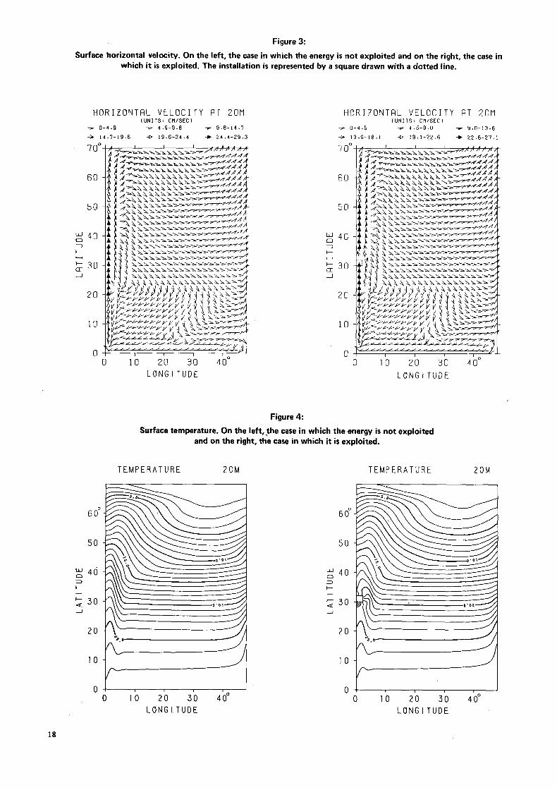
Figure 3: Surface horizontal velocity. O n the left, the case in which the energy is not exploited and on the right, the case in

which it is exploited. The installation is represented by a square drawn with a dotted line.

HORIZONTFIL VELOCITY FIT 20M (UNITS: C W S E C )

7 0-4.9 v 4.9-9.8 T 9.8-14.7 -3 14.7-19.6 -D 19.6-24.4 + 24.4-29.3

70

60

50

t - - + 30 a _J

20

10

fl

HORIZONTAL VELOCITY AT 2CM (UNITS: Ctl/SECI

0-4.5 v 4.5-9.0 T 9.0-13.6 + 13.6-18.1 + 18.1-22-6 -t 22.6-27.1

Figure 4: Surface temperature. O n the left,the case in which the energy is not exploited

and on the right, the case in which it is exploited.

TEMPERATURE 20M TEMPERATURE 20M

6 0"

50

2 40 3 c - 4. 30 _I

20

6 0"

50

40 3

2 30

o ! IO 20 3b 42

I 0

L O N G I T U DE

0 0 IO 20 30 40'

L O N G I T U DE

18

Discussion’ S.M. ul-Haq

H.U. Roll

Thank you Mr. Chairman. I hope that Dr. Takano is able to understand what I a m going to say.

Your talk, Dr. Takano, has been very interesting to us here in IOC in view of the discussions w e had the other day on whether or not it would be worthwhile for IOC to undertake studies on ocean energy. I personally had the opinion that extracting energy out of the ocean was purely a technical problem, and that it was beyond the interest and capacity of IOC. But w e have learnt from your talk that there is still another problem to be solved, namely that w e should k n o w what would happen to the ocean if energy were to be extracted from it on a large scale; and from your talk I got the impression that this must be done by theoretical modelling by mathematical models. If this is the case, h o w can IOC which is organizing world wide and regional research exercises in the oceans-to get to k n o w more about the nature of the oceans contribute to such studies? Y o u ended up by saying that fundamental research is needed on the nature of the ocean; the only contribution I can envision at present is that IOC could perhaps provide data for the verification or the testing of such models. Thank you.

K. Takano

Thank you for your comments.

H. Postma

I d o not want to comment on Professor Roll’s remarks as I did so a few days ago; but I have a question: you did consider tidal friction as a source of energy, but you did not discuss the energy that can be derived by using the difference between high and low sea levels, as is done, for example, in that enclosed basin along the French coast in the Rance. Have you any idea or suggestion about the amount of energy that could be derived from that tidal difference?

K. Takano

The energy dissipated by friction is a portion of the tidal energy. The global aspect of the tides should be unchanged if the energy harnessing is less than this amount of energy which is thrown away, in a sense. Since the tidal dif- ference is a phase of the tidal energy, the upper limit of the energy which could be derived from the tidal dif- ference could be considered to equal the energy dissipated by friction.

H. Postma

So as I understand you, the tidal height difference-or the energy that can be derived from that-is included in the tidal friction?

Thank you Mr. Chairman. Dr. Takano has touched upon very important aspects of the subject of ocean energy. There is one particular aspect I would like to k n o w his views on, and that is the possibility of artificially enhancing upwelling in certain regions for the purpose of increasing biological production in these areas. I wonder if Dr. Takano can throw more light on this aspect if it is not outside the scope of his lecture. Thank you.

K. Takano

I hope to have a chance to talk about this aspect some other time, although I have no thorough knowledge of it.

B.A. Nelepo

I would like to ask a question of Dr. Takano. I was very optimistic on the use of ocean enciyy before I saw the first table of your paper. W h e n you showed the various energy contributions of the total heat balance, I realized that this is. in principle, a more complex way for the transformation of solar energy. T h e ocean accumulates solar energy and then we, with very low efficiency, must extract this energy from the ocean. Furthermore, there are ecological implications in the use of ocean energy. T h e question therefore is whether the present ways of direct transformation of solar energy into electricity are the most promising. Of course, I realize that in future w e will have to use the energy of the ocean. Thank you.

K. Takano

I a m not m u c h of a specialist o n the direct conversion of solar energy, so would not like to say whether direct conversion is the most promising process.

J. Stromberg

Dr. Takano, in your tables of the potential energy from various sources, I guess that you have calculated these o n a global scale, and this, of course, does not mean that all this energy is available for practical use. It would therefore be interesting to have an approximate idea of h o w much of this could really be utilized. Is it 50%or is it less or more?

K. Takano

T h e figures in the table are, as it were, theoretical, oceano- graphical limits disregarding economical and financial circumstances. T h e amount of ocean energy really utilizable would depend, to a large extent, o n many other factors such as the price of petroleum and other energies, and the effect of such energy utilization on our environment. It is therefore very difficult to have an idea, even a rough idea, of h o w much of the ocean energy could be utilized in the near future; I guess several tens of percent might be possible.

K. Takano

Yes.

1. Names and titles of speakers are given at the end of the publica- tion.

19

R. Zoeliner K. Takano

Y o u introduced to us several methods of getting energy from the oceans, and I want to ask your opinion about the possibility of extracting energy from the Ocean by thermocouples.

Studies are currently being made in regard to a large number of new techniques, involving use of thermocouples, piezoelectric generators, etc., but it would be unrealistic to count on them in the short-term future.

N.J. Campbell

Dr. Stuart Godfrey, the author in absentia of our third paper this afternoon, took his undergraduate and graduate studies at the University of Tasmania and his doctorate at Cambridge University, England. H e is currently a senior research scientist in Fisheries and Oceanography at the Commonwealth Scientific and Industrial Research Organi- zation of Australia.

His speciality is the theory of modelling of ocean cur- rents. H e hasdevoted much of his time to the East Australian current and the mesoscale anticyclonic eddies that it generates. Recently he has been examining the interaction between variability of the Equatorial circulation in the

Western Pacific and the El Niiio phenomenon. H e has produced a major paper on the mechanism linking El Niiio with events in the Western Equatorial Pacific. Dr. Godfrey's interest and expertise has brought him to

the United States on several occasions, providing him an opportunity of working with other colleagues in the same field.

As I mentioned, owing to illness, Dr. Godfrey could not attend our session. His paper will be presented by Dr. David Rochford, head of the Australian Delegation, who, on short notice, very kindly offered to present Dr. Godfrey's paper.

May I present Dr. Rochford.

20

Short-term change: a physical oceanographer's point of view

J. S. Godfre y, CSIRO Division of Fisheries and Oceanography P. 0. Box 2 I, Cronulla, NS W 2230 Australia

Introduction

At any given place in the ocean, the sea surface tempera- ture varies annually, being warmer in summer and cooler in winter. However, this average pattern is generally disturbed by anomalies of sea surface temperature (SST) -regions typically one or 'two thousand kilometres across, and lasting for a few months, in which SST is consistently above or below the average for that time of year. These anomalies can disturb the air flow above it, causing short- term climate change? A n d what physical mechanisms are likely to create SST anomalies in these regions? A t present, w e cannot answer either question with great certainty; but enough is known so that a review o n the subject seems appropriate.

Oceanic regions of importance

(a) The Gulf Stream outflow Ratcliffe and Murray (1970) examined sea surface tempera- ture anomaly data in the Atlantic Ocean, from 1876-1968, (with wartime gaps). They found that the region south of Newfoundland, where the Gulf Stream decayed, was particularly likely to have strong SST anomalies. They examined anomalies in this region for each month of the year. For instance, in September there were 1 1 years in which SST was more than l0C lowerthan usual throughout the region, and 13 years in which SST was more than l0C higher than usual (Fig. 1). October pressure maps for all the cold SST years were then averaged, and compared with the average of October maps for all 70 years. T h e result is shown in Fig. IC: a high pressure region centred on Scandinavia is found, presumably caused by the cold anomaly. This is confirmed by looking at a similar m a p for the Octoben of all years with warm September anomalies. It is close to being the negative of the pattern for cold anomalies, confirming the belief that a real phenomenon has been found. In general, throughout the year, it was found that SST's off Newfoundland have useful predictive power for European weather the follow- ing month.

Thus the region south of Newfoundland is one important area of the ocean, climatologically. It is also the area where the Gulf Stream weakens and breaks up: SST's there must depend, much more than in other parts of the Atlantic, on changes in whatever forces drive the Gulf Stream. By analogy, w e might expect a similar region subject to large SST anomalies east of Japan, where the Kuroshio breaks up: Davis (1976) has shown that this is the case. In the southern hemisphere, w e might expect the three regions off Southern Brazil, south of South Africa, and off N e w South Wales to be particularly subject to large SST anomalies, and that these might be influential o n weather elsewhere.

(b) The tropical Atlantic A second Ocean region whose SST anomalies have been shown to influence climate is the eastern tropical Atlantic. This region appears to affect rainfall in northeast Brazil, which is an area prone to frequent droughts and floods, particularly in January-March. Markham and McLain (1977) devised an index of average January-March rainfall in this region, and correlated it with SST in the tropical Atlantic (Fig. 2). In December, a region in the Eastern Atlantic that is highly correlated with rainfall in Brazil in the following January-March. develops. This region can be seen to move westward and weaken in the following months. Thus the equatorial Atlantic, particularly near its eastern side, is a useful rainfall predictor for Brazil.

(c) The equatorial Pacific However, the strongest example of SST anomalies influenc- ing weather is associated with the socalled "Southern Oscillation". Sea level pressure (SLP) shows anomalies throughout the tropical belt, that follow a single pattern around the world (Fig. 3). In this pattern, when the pres- sure is low over Indonesia, Australia and Africa, it is high over the Pacific, and vice versa. This pattern-the "Southern Oscillation"-has typical periods of several months to several years. It accounts for a large number of related climate anomalies. For example, if Fig. 3 is regarded as a pressure map, w e would expect winds from the north over Eastern Australia when the Southern Oscillation Index is high. These winds would be likely to bring moist air from the Coral Sea over East Australia, producing rain. Figure 4 suggests that such a relation m a y indeed be valid. In particular, 1940 marked a change from anomalously high to anomalously low pressure at Darwin; it also marked a change from dry to wet conditions in East Australia. In short, the Southern Oscillation is an extremely important global climatic phenomenon.

It has been found that the Southern Oscillation is intimately tied to SST anomalies in the eastern equatorial Pacific. In particular, the average temperature in the shaded strip in Fig. 3 is shown as a function of time in Fig. 5; the Southern Oscillation Index is also shown. Evidently, the correlation between the two is very close. Meteorologists believe that SST in the eastern tropical Pacific plays a central role in the mechanism governing the Southern Oscillation. To summarize, SST anomalies in the tropics-and

particularly the eastern tropics-appear to be particularly influential for short-term climate change. In at least one case the outflow region of a western boundary current also affects climate. However, little systematic study has yet been done on the correlation of SST anomalies over the ocean as a whole with climate variations over land areas.

21

Physical mechanisms for sea surface temperature change

The second question raised at the start of this talk was: what physical mechanisms are likely to cause SST changes in the regions of importance? There are a number of possi- bilities, but w e shall discuss only three.

(i) Mixed layer formation Over m u c h of the ocean, average currents are quite weak, so that changes in temperature are primarily due to local effects-incoming solar radiation, exchange of sensible and latent heat with the atmosphere, and wind mixing. W h e n these effects operate alone, they produce an annual cycle of temperature as shown in Fig. 6. Starting in spring, a layer of w a r m water appears at the surface; the surface mixed layer increases in temperature and decreases in depth through till late summer. W h e n fall cooling sets in, the mixed layer cools and deepens progressively ~~~~ through ~

winter. T h e deepening is caused both by convective over- turning and by wind mixing. Note that temperature changes below the winter mixed layer show no clear seasonal cycle. If w e are to understand h o w SST anomaliesoccur anywhere in the ocean, it is essential that w e should be able to des- cribe quantitatively the mixed layer response to these influences.

Substantial progress has been achieved in this direction in recent years. A good example is seen in Fig. 7 which shows wind speed, solar and back radiation, SST, and pro- files of temperature for a 12-day period in June 1970, at 50°N in the North-East Pacific Ocean (from Denman and Miyake 1973). The dashed line in Fig. 7c is the observed SST, the full line, the prediction from a very simple numerical model. This model is so simple that w e can understand it qualitatively by inspection: on 14, 1 8 and 21 June, the surface temperature takes a sharp rise, both in reality and in the model. Looking u p to Fig. 7a and 7b. w e see that these days are not usually sunny, but the wind speed is unusually low. Looking d o w n at Fig. 7d, w e can n o w understand w h y SST rose sharply on these days. O n calm days the sun's heat enters the top few metres, and is not carried d o w n by wind mixing. Conse- quently, a thin surface layer is formed, which absorbs all incoming radiation a d heats u p rapidly. W h e n the winds increase again, this heat is mixed into the rest of the water column, and surface temperature falls. Conversely, one of the major causes of long-lasting SST anomalies is believed to be strong winds. Thestrength of wind mixing is believed to increase as the cube of the wind speed; so a gale will mix the ocean to unusually great depths over wide areas, thereby causing SST to fall substantially.

S o m e recent works have shown that the model used by Denman and Mijake has several shortcomings, not revealed in- Fig. 7. However, observational and theoretical work o n ocean mixed layer behaviour are being vigorously pursued around the world, so these shortcomings will probably be corrected in the coming years.

(ii) Wave-like phenomena in the eastern tropical oceans T h e purely local effects just discussed are confined, in the eastern tropics, to the top 40 metres or less, but in the tropics the entire thermal structure d o w n to about 400 metres is subject to continuous vertical motions. W h e n the motion is upwards, temperatures fall at all depths, and in particular at the surface. This "upwelling"

(and its converse, "downwelling") occurs through the action of certain waves that are excited by changes in the wind field. The easterly winds along the equator are particularly crucial: if they slacken for a few months, the w a r m water that generally lies at the western side of the equatorial Pacific surges eastward, causing the thermocline to deepen in the eastern equatorial Pacific. This surge takes only about four weeks to reach South America (Fig. 8a). A wave of downwelling then moves north and south along the American coast (Fig. 8b). thus creating areas of deep thermocline and raised SST near the coast. Further down- welling waves extend the area of deepened thermocline westward (Figs. 8c, 8d); the westward motion being most rapid near the equator,

This picture, suggested by Godfrey (1975) and further investigated by McCreary (1976) and Hurlbert, Kindle and O'Brien (1976), accounts quite well for the broad details of the El Niiio phenomenon. In particular, sea temperatures do appear to rise, in a broad region along the American coast and along the equator, a month or two after the mid-Pacific equatorial easterlies slacken (Wyrtki, 1977).

(i i i ) Upwelling and advection in the outflow

Sea surface temperature in the outflow regions of western boundary currents is certainly influenced by the purely local effects mentioned earlier-wind mixing, solar heating, etc.; but it seems probable that the fluctuations of the cur- rents themselves are the dominant influence. Unfortunately, these fluctuations can be extremely complex. Figure 9 shows a photograph, taken in infrared light from the TI ROS-N satellite, of the East Australian Current. A w a y from clouds and land, darker tones indicate warmer sea surface temperatures. Sharp fronts and long, thin ribbons of w a r m water are frequently seen associated with eddies in the East Australian Current. Even to evaluate the area- average SST in such a region is very difficult; to explain the variations of that average in terms of changes in the winds or heating involves a degree of understanding of western boundary currents that is not yet available. Thus for the time being at least, w e must regard anomaly patches such as those south of Newfoundland or off East Australia as being "non-forecastable".

of western boundary currents

Conclusions

It seems reasonable to hope that, given appropriate real- time data over the global ocean, SST in theeastern tropical oceans can be forecast for perhaps two months in advance, using our understanding of upwelling and of local effects on SST. If so, it would considerably enhance the value of relations such as that of Markham and McLain-i.e. if the December SST anomaly that relates to Brazil rainfall could itself be forecast a month or so ahead, the time available for remedial action would be increased. Similar remarks apply to east Pacific temperature and the Southern Oscillation.

There are very large further areas of ocean where SST anomalies are driven primarily by local effects-namely the regions away from land boundaries and from the equator. For these areas too, meaningful SST forecasts can probably be prepared if these turn out to be useful for climatic purposes. However, SST anomalies in the outflows of western boundary currents will probably remain unforecastable for some time.

22

There is an important proviso that must be satisfied before prediction of SST anomalies becomes effective, namely, that appropriate real-time data is available. This talk has emphasized the crucial role played by the wind field in determining SST's: merchant ship reports are too scanty for real-time use,so that another source is necessary. During the three months that SEASAT was aloft, the capability of a satellite sensor for measuring ocean wind speed and direction was proven (Jones et al., 1979). It is strongly to be hoped that such an instrument will be put into space again in the near future. With such an instru- ment, prediction of SST anomalies over wide areas m a y be possible, while without it SST anomaly prediction is considerably less likely to be effective.

Other data essential to SST forecasts are radiation inputs; satellite cloud information is probably adequate for this purpose. Information on air temperature and humidity are also desirable, but they are not likely to be obtainable; it is, however, quite likely that climatological information will prove adequate for this purpose.

References

Davis, R.E. 1976. Predictability of sea surface temperature and sea level pressure anomalies over the North Pacific Ocean. J. Phys. Oceanogr. Vol. 6, p. 249-266.

Denman, K.L.; Miyake, M. 1973. Upper layer modification at ocean station"Papa": Observations and simulation. J. Phys. Oceanogr. Vol. 3, p. 185-196.$

Godfrey, J.S. 1975. O n Ocean Spindown I: a linear experi- ment. J. Phys. Oceanogr. Vol. 5, p. 460-475.

Hurlbert, H.E.; Kindle, J.C.; O'Brien, J.J. 1976. A numeri- cal simulation of the onset of El Niiio. J. Phys. Oceanogr. Vol. 6. p. 632-645.

Jones, W.L.; Black, P.G.; Boggs, D.M.; Bracalente, E.M.; Brown, R.A.; D0me.G.; Ernst,J.A.; Halberstam,l.M.; Overland, J.E.; Peteherych, S.; Pierson, W.J.; Wentz, F.J.; Woiceshyn, P.M.; Wurtele, M.G. 1979; Seasat scatterorneter: results of the Gulf of Alaska Workshop. Science Vol. 204, p. 1413-1415.

McCreary, J. 1976. Eastern tropical ocean response to changing wind sytems: with application to El Niiio. J. Phys. Oceanogr. Vol. 6, p. 632-645.

Markharn, C.G.; McLain, D.R. 1977. Sea surface tempera- ture related to rain in Ceara, northeastern Brazil. Nature Vol. 265, p. 320-323.

Pittock, A.B. 1975. Climatic change and the patterns of Australian rainfall. Search Vol. 6, p. 498-504.

Ratcliffe, R.A.S.; Murray, R. 1970. N e w lag associations between N. Atlantic sea surface temperature and European pressure applied to long-range weather forecasting. Q.J. Roy. Met. Soc. Vol. 96, p. 226-246.

Turner, J.S. 1973. Buoyancy effects in fluids. Cambridge, Cambridge University Press, 367 pp.

Wright, P.B. 1977. The Southern Oscillation-patterns and mechanisms of the teleconnections and the per- sistence, Hawaii Institute of Geophysics Report

Wyrtki, K. 1977. Sea level during the 1972 El Niiio. HIG-77-13.

J. Phys. Oceanogr. Vol. 7, p. 779-787.

23

Figure 1: (a) Mean pattern of sea surface temperature anomaly ("C) in September

based on years with a significant negative (cold) SST anomaly area off Newfoundland. Positions of anomaly centres and last two figures of year shown:

negative anomaly > 2O C; A negative anomaly between 1 and 2'C; X position and intensity less certain.

(b) As for Figure 1 (a), but positive (warm) SST anomaly. (c) Mean surface pressure anomaly (mb) in October for the years with a

negative September SST anomaly off Newfoundland as shown in Figure l(a).

(d) As for Figure 1 (c), but for years with a positive September SST anomaly.

24

Figure 2: Correlation between SST and January-February-March rainfall indices in Cear5, northeastern Brazil.

A n area of high coefficient of correlation appears off the African coast in November, becomes strong in December, moves westward with the South Equatorial Current

during January, February and March, and disappears in April. From Markham and McLain (1977).

LI nr

,. I, .L. 1. Q I

U. .> ,. 0.

25

Figure 3: Correlation coefficients (X 100) of sea level pressure anomaly with the "Southern Oscillation Index". From Wright (1977). The Southern Oscillation Index, and the average sea surface temperature in the

shaded box, are shown as a function of time in Figure 5.

Figure 4: (a) Cumulative mean annual rainfall anomalies, East Australia. (b) Cumulative sea level pressure anomaly, Darwin; (sea level pressure anomaly at

Darwin may be used as a "Southern Oscillation Index"). From Pittock (1975).

L

C E E -2

-4

-1

0

I)

E +1

+2

3 a ) C u m u l a t e m e a n annual

rainfall anomalies. , East Australia.

b ) C u m u l a t i v e pressure a n o m a l y , Darwin. (Southern oscillation index .)

I I 1 I 1920 30 40 50 60 70

26

Figure 5: (a) Sea surface temperature, 90°-180°W, 1O0N-lO0S, 1949-1970. (b) Southern Oscillation pressure index, 1949-1975.

- (a) SST (inverted) 90" - 180' W, 1O"N - 10's -

n -

+ 2 - -

I950 1955 1960 I965 19 70 1975 1 1 1 1 1 1 1 1 1 1 1 1 1 1 1 1 1 I 1 1 1 1 1 1 1 1 1 1

(b\ SO PRESSURE INDEX +2 -

m x [r - I a

- - 2 -

Figure 6: (a) A typical annual heating and cooling cycle observed in an area of small advection (the subarctic

Pacific) compared with (b) the variation of temperature with depth in the same region. Isotherms are marked in F. From

Turner (1973).

0 Jan Feb Mar. Apr May J u n e July A u g Sept Oct Nov Dec.

21

Figure 7: Observed wind speed, Ulo, 1 0 m above the sea surface, 13-24 June 1970. Solar and back radiation, for the same period. Sea surface temperature, as observed (dashed line) and as predicted (full line).Note that major temperature rises occur at times of low wind speed. Observed and predicted temperature profiles (each 1 2 hour). From Denman and Miyake (1973).

b ------- RACK RADIATION - SOLAR RADIATION

I C

Figure 8: If the easterly winds inside the dashed line relax for a few months a wave of downwelling causes the thermdine to deepen, first along the eastern equatorial Pacific (Figure 8(a)); then along the American coast (Figure 8(b)). The area of deepened thermocline then spreads westward, through the action of further downwelling waves (Figures 8(c), 8(d)).

AREAS OF DEEPENED THERMOCLINE AFTER RELAXATION O F EQUATORIAL WINDS

(a) 4 weeks Cb) 6 weeks

28 CC) 12 weeks Cd 1 24 weeks

Figure 9: Typical TI ROS-N infra-red satellite photo of the East Australian Current region. Over cloudfree ocean areas, dark tones, indicate warm temperatures (for 20 August 1979). The average temperature in such an area is difficult to assess, let alone predict.

29

N.J. Campbell

Our final speaker today is Dr. David Cushing. Dr. Cushing received his formal education at Balliol

College, Oxford University. Soon after World War I I he joined the Ministry of Agriculture, Fisheries and Food at Lowestoft, England. His research and advanced studies on fish stock management have made him one of the foremost scientists in this field. Dr. Cushing pioneered such tech- niques as acoustic estimation of fish populations and fish population dynamics. H e has also carried out extensive studies on plankton and herring not only in the h o m e waters of the United Kingdom but also off South Africa, in the Indian Ocean and in the Pacific.

H e is an Honorary Professor of the University of East Anglia and has lectured extensively abroad including the University of Wisconsin, University of Washington and Oregon State University in the United States. H e is presently the Deputy Director of the Fisheries Laboratories at Lowestoft, a post which he has held since 1974.

Dr. Cushing is the author of numerous papers and two important books: one on Marine Ecology and Fisheries, the other on Fisheries Resources of the Sea and their Management. In 1977, he was elected a Fellow of the Royal Society in honour of his scientific achievements.

Dr. Cushing.

30

Production in the central gyres of the Pacific D. H. Cushing,

Ministry of Agriculture, Fisheries and Food, Directorate of Fisheries Research, Fisheries Laboratory,

Lowestoft, Suffolk NR33 OHT, U.K.

introduction

Production in the centres of thesubtropical gyres is always low, 0.1 -0.5 g C/m2/d, and m a y continue throughout the year with little variation, though Riley (1957) and Ryther and Menzel (1960) showed that in the Sargasso Sea there was more productionduringthe winter months. Production, as estimated by the radiocarbon method, continues at the surface, yet nutrient concentrations there are often so low as to be undetectable. Of course, the surface is the wrong place to look, perhaps because the light is too strong; there is a chlorophyll m a x i m u m near the bottom of the euphotic layer (for example see Shulenberger, 1978) and it has often been suggested that this relatively deep layer (about 100 m) is fertilized from below by various hydrodynamic mechanisms.

Because there is little variation in production with time, Cushing (1959) Suggested that a steady-state system exists where, for example, the reproductive rate of the algae is balanced by their grazing mortality, and analogous rates are balanced at higher trophic levels in the system. Under such a system one would expect the uptake of nutrients by algae to be balanced by immediate regeneration. Cushing (1971) pointed out that any quantity of nutrients observed in the euphotic layer comprises preddminantly regenerated material, but it is difficult to imagine that regeneration might in fact match the uptake unless the reproductive rate was well restrained by a nutrient defi- ciency, and then w e might expect less nutrients to be transferred to higher trophic levels and therefore less immediate regeneration. A n extension of this argument might suggest that regeneration did not take place at all.

Another remarkable point is that there appears to be a larger biomass of animals than algae. A s will be shown, this is not always true, but happens often enough to raise a question. If true, then the reproductive rate of the algae must be fairly high to provide that quantity of animals with food, which might suggest a steadystate system, independent of externally supplied nutrients.

In this paper w e examine production in the cehtres of the tropical gyres to try to understand the relatively deep chlorophyll maxima, the high ratio of herbivores to algae, and the nature of a possible steady-state system.

The deep chlorophyll layer

T h e existence of the deep chlorophyll layer in the sub- tropical ocean has been well known for a long time (Venrick et a/. 1973 summarizes the historical evidence). Figure 1 shows the vertical distribution of chlorophyll a, nitrate, a m m o n i u m and phaeophytin at their B stations (see below) in the centre of the South Pacific subtropical gyre. T h e chlorophyll layer was distributed between 80 and 140 m with a rough m a x i m u m between 100 and 120 m. Th e depth of the euphotic layer (1 % of subsurface irradiance) was at about 100 m. Th e chlorophyll layer extends below the euphotic layer as defined in this way, and some slow production m a y take place below this somewhat arbitrary level which m a y be difficult to deter- mine in the very clear oceanic water. Nitrate values are low and variable in the first 100 m, but increase below that level. T h e distribution of a m m o n i u m with depth is quite different, being evenly distributed with depth and somewhat less variable. T h e phaeophytin distribution matches the chlorophyll distribution to some degree. T h e deep chlorophyll layer supports production at low nutrient and irradiance levels.

The ratio of animals to plants

Table 1 gives some examples of the quantities of animals and plants in the same units from the tropical and sub- tropical ocean away from the coastal upwelling areas. It should be noted that the methods of sampling are diverse, that there m a y be some differences in the classification of

Table 1

The ratio of animals to plants in the tropical and subtropical ocean ~~

Atlantic Ionian Sea Pacific equatorial upwelling Sargasso Sea Equatorial upwelling S. Atlantic

Phytoplankton 19.0 6.8 31.35 3.33 2.93 3.12 0.3-0.5 180 108 0.01 12 Herbivores 36.6 48.7 6.20 2.00 2.98 2.50 499 12 0.021 6 Total zooplankton 54.0 58.4 13.50 7.21 6.99 7.20 2.23 838 22

Units (rng/m3 dry wt.) (g/m2 dry wt.) (9. C/rn2) (ca~/m3) (rngll dry wt.)

Zooplankton Phytoplankton 2 .a4 8.59 0.63 2.77 2.39 2.31 4.46 4.66 0.20 1.93

(Greze, 1970) (Vinogradov and Shushkina, (Cushing, (Petipa, 1978) (Meteor expdn. 1977) 1959) Cushing, 1962)

31

Figure 1: Distribution of chlorophyll a, nitrate, a m m o n i u m and phaeophytin at the B stations (Venrick et al., 1973).

0 - O . l - / 1 _ 0 _ I

Om2 -1

"'1 00 Oal 0-, -a

"'-1 m o

"'1

3 -

0 100 200 Chl'a'

0 100 200

NO3

32

Figure 1 (continued)

1.0 -

* 6)

1.0 -

2.0 -t Q2 -1

o-2-l

I I F

2.0-l m 1.0-1

I 1 c

0 100 200

NH4

0.1 "'1 -

"-1 0 100 200

Phaeo

33

herbivores, and that zooplankton and nekton m a y be dif- ficult to separate. There are two observations, both in the equatorial upwelling region, where the ratio of animals to plants is less than one, but there are eight observations where the ratio is greater than unity. T h e absolute quanti- ties of animals are quite high but less than those in the regions of coastal upwelling. To maintain such a ratio, the reproductive rates of the algae must be perhaps many times greater than those of the herbivores; the respiration rate of the herbivores is high because they are small and the water is warm, and the generation time is probably short. Therefore, the algal reproductive rate must be fairly high under conditions of low nutrients.

Methods

Th e data report on the Climax I1 expedition (27 August- 13 October 1969)from Scripps Institution of Oceanography (SI0 reference 75-6) gives the physical, chemical and bio- logical information from a set of stations (A) in the centre of the North Pacific gyre and a set (B) in the centre of the South Pacific gyre (the work was reported by Venrick et al., 1973). There were ten A stations (26 August- 6 September) and six B stations (3-8 October) where samples were taken continuously as the ship drifted. Samples of chlorophyll a (corrected for phaeophytin) and radiocarbon measurements were made at a range of light intensities (about 1%. 1.5%. 2.3%, 5.4%, 20%, 40% and 50% of the subsurface irradiance). At the same time samples for nitrite, nitrate, ammonia, silicate and phosphate were collected, sometimes at the same depths and some- times at standard depths (in which case interpolated estimates were used). Micro-zooplankton was collected by p u m p (from five depth ranges: 0-20 m . 21 -41 m, 42-62 m, 63-1 04 m and 105-1 69 m); the samples were passed through, three filters of mesh sizes 35 um , 103 u m and 363 um. Zooplankton biomass was sampled with an Isaacs-Kidd pelagic trawl from about 300 m ; at the A stations, macro- zooplankton and fish were sampled with an Isaacs-Kidd midwater trawl d o w n to 3,500 m . Where possible, data from the night stations of animal samples have been used because, owing to vertical migration, more animals will be near the surface at night, including most of those which, during the day, are found as far d o w n as 3,500 m.

Eppley et al. (1973) studied North Pacific plankton dynamics and sampled ATP (adenosine triphosphate) using Holm-Hansen's method (1969, 1970); "living" carbon was

T a b k ,

estimated to be 250 times the particulate ATP. Their paper also gives a "living" carbon/chlorophyll ratio with depth, ranging from 150-200 in the top 60 m . to 35-60 in the chlorophyll m a x i m u m layer. The decline of the ratio with depth m a y well be an effect of too bright light in the upper parts of the euphotic layer. Their Figure 3 shows the dependence of this ratio with depth and I have used interpolated values where needed. For each station, "living" carbon in m g C/m2 was calculated for the euphotic layer and, as the radiocarbon measurements were expressed as mgC/m2/12 h.(from6 hourdeterminationsfrom1200 h. to 1800 h.), the ratio or productivity to stock of carbon could be used to estimate the reproductive rate of the algae. This ratio A is Po (exp Rt-l)/Po, where Po is the initial stock of carbon in the radiocarbon experiment and R is the reproductive rate of the algae. Then R = In(A+l). T h e method depends entirely upon the estimate of "living" carbon, but if biased, the differences are c o m m o n in the subsequent treatment. Furthermore, G=R-I n(P, /Po), where Po is the initial value of algal stock on one day and PI that on the next, and G is the instantaneous mortality due to grazing.

The quantity produced each day, PR, and the quantity eaten, PG, are given by:

both being in g C/m2/d. Goldman and McCarthy (1978) show that the ratio N/C = 0.16 was constant (which is effectively the Redfield ratio) in algae grown under con- ditions of a m m o n i u m limitation. Hence the quantities in g C/m2 or g C/m2/d can be converted to g N / m 2 or g N/m2/d. From experiments on Calanus grazing on Biddulphia sinensis, Corner (1973) has estimated the proportion of ration converted to growth, soluble excretion and faecal pellets,all of which can be applied to the quantity grazed, PG, and expressed as g N/m2/d.

Results

The average conditions of production at the A stations (in the North Pacific gyre) and at the B stations ( in theSouth Pacific gyre) are given in Table 2. The algal stock in the northern gyre is nearly 50 % greater than that in the southern one, but the estimate is somewhat more variable.

The production parameters in the North Pacific gyre (A stations) and in the South Pacific gyre (B stations)

Rate f meal Rate of gowth of Rate soluble pellet

excretion I) rod ucti on herbi vores R G pR pG Algal Stock

g C/m2 g Clm2/d g C/m21d

(f 0.285) (f 0.18) (f 0.57)

(f 0.148) (f 0.15) (+ 0.30)

10 A 0.746 0.44 0.43 0.328 0.32 1

7 B 0.521 0.27 0.21 0.141 0.1 09

g N/m2/d g N/rn2/d g N/rn2/d g N/rn2/d g N/rn2/d 10 A 0.0525 0.0514 0.0184 0.01 93 0.01 37 7 B 0.0226 0.01 74 0.0062 0.0065 0.0046

34

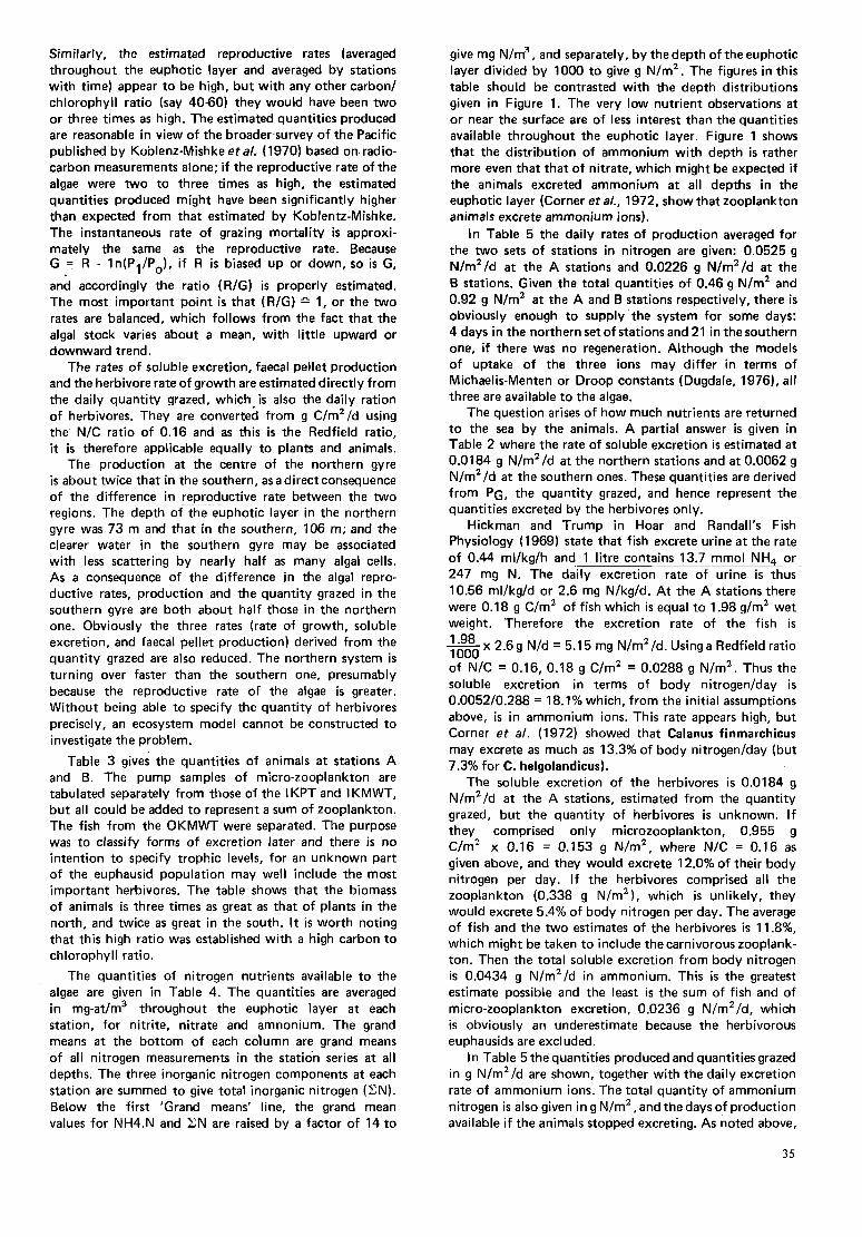
Similarly, the estimated reproductive rates (averaged throughout the euphotic layer and averaged by stations with time) appear to be high, but with any other carbon/ chlorophyll ratio (say 4060) they would have been two or three times as high. The estimated quantities produced are reasonable in view of the broader survey of the Pacific published by Koblenz-Mishke er al. (1970) based on radio- carbon measurements alone; if the reproductive rate of the algae were two to three times as high, the estimated quantities produced might have been significantly higher than expected from that estimated by Koblentz-Mishke. The instantaneous rate of grazing mortality is approxi- mately the same as the reproductive rate. Because G = R - In(P1/Po), if R is biased up or down, so is G, and accordingly the ratio (R/G) is properly estimated. The most important point is that (R/G) e 1, or the two rates are balanced, which follows from the fact that the algal stock varies about a mean, with little upward or downward trend.

T h e rates of soluble excretion, faecal pellet production and the herbivore rate of growth are estimated directly from the daily quantity grazed, which-is also the daily ration of herbivores. They are converted from g C/mZ/d using the N/C ratio of 0.16 and as this is the Redfield ratio, it is therefore applicable equally to plants and animals.

The production at the centre of the northern gyre is about twice that in the southern, as a direct consequence of the difference in reproductive rate between the two regions. The depth G-the euphotic layer in the northern gyre was 73 m and that in the southern, 106 m ; and the clearer water in the southern gyre m a y be associated with less scattering by nearly half as m a n y algal cells. A s a consequence of the difference in the algal repro- ductive rates, production and the quantity grazed in the southern gyre are both about half those in the northern one. Obviously the three rates (rate of growth, soluble excretion, and faecal pellet production) derived from the quantity grazed are also reduced. The northern system is turning over faster than the southern one, presumably because the reproductive rate of the algae is greater. Without being able to specify the quantity of herbivores precisely, an ecosystem model cannot be constructed to investigate the problem.

Table 3 gives the quantities of animals at stations A and B. The p u m p samples of micro-zooplankton are tabulated separately from those of the IKPT and IKMWT, but all could be added to represent a s u m of zooplankton. T h e fish from the OKMWT were separated. The purpose was to classify forms of excretion later and there is n o intention to specify trophic levels, for an unknown part of the euphausid population m a y well include the most important herbivores. The table shows that the biomass of animals is three times as great as that of plants in the north, and twice as great in the south. It is worth noting that this high ratio was established with a high carbon to chlorophyll ratio.

The quantities of nitrogen nutrients available to the algae are given in Table 4. Th e quantities are averaged in mg-at/m3 throughout the euphotic layer at each station, for nitrite, nitrate and amnonium. The grand means at the bottom of each column are grand means of all nitrogen measurements in the station series at all depths. The three inorganic nitrogen components at each station are s u m m e d to give total inorganic nitrogen (XN). Below the first 'Grand means' line, the grand mean values for NH4.N and ZN are raised by a factor of 14 to

give m g N/m3, and separately, by the depth of the euphotic layer divided by 1000 to give g N/m2. T h e figures in this table should be contrasted with the depth distributions given in Figure 1. The very low nutrient observations at or near the surface are of less interest than the quantities available throughout the euphotic layer. Figure 1 shows that the distribution of a m m o n i u m with depth is rather more even that that of nitrate, which might be expected if the animals excreted a m m o n i u m at all depths in the euphotic layer (Corner er al., 1972, show that zooplankton animals excrete a m m o n i u m ions).

In Table 5 the daily rates of production averaged for the two sets of stations in nitrogen are given: 0.0525 g N/m2/d at the A stations and 0.0226 g N/m2/d at the B stations. Given the total quantities of 0.46 g N / m 2 and 0.92 g N/mZ at the A and B stations respectively, there is obviously enough to supply the system for some days: 4 days in the northern set of stations and 21 in the southern one, if there was no regeneration. Although the models of uptake of the three ions m a y differ in terms of Michaelis-Menten or Droop constants (Dugdale, 1976), all three are available to the algae.

The question arises of h o w m u c h nutrients are returned to the sea by the animals. A partial answer is given in Table 2 where the rate of soluble excretion is estimated at 0.0184 g N/m2/d at the northern stations and at 0.0062 g N/m2/d at the southern ones. These quantities are derived from PG, the quantity grazed, and hence represent the quantities excreted by the herbivores only.

Hickman and T r u m p in Hoar and Randall's Fish Physiology (1969) state that fish excrete urine at the rate of ~ ~ _ _ ~ 0.44 ml/kg/h ~- ~ and -- 1 litre contains 13.7 mmol NH, or 247 m g N. The daily excretion rate of urine is thus 10.56 ml/kg/d or 2.6 m g N/kg/d. At the A stations there were 0.18 g C / m Z of fish which is equal to 1.98 g/m2 wet weight. Therefore the excretion rate of the fish is m x 2 . 6 g N/d = 5.15 m g N/mz/d. Using a Redfield ratio 1000 of N / C = 0.16, 0.18 g C/m2 = 0.0288 g N/m2. Thus the soluble excretion in terms of body nitrogen/day is 0.0052/0.288 = 18.1% which, from the initial assumptions above, is in a m m o n i u m ions. This rate appears high, but Corner et a/. (1972) showed that Calanus finmarchicus m a y excrete as m u c h as 13.3% of body nitrogedday (but 7.3% for C. helgolandicus).

T h e soluble excretion of the herbivores is 0.0184 g N/m2/d at the A stations, estimated from the quantity grazed, but the quantity of herbivores is unknown. If they comprised only microzooplankton, 0.955 g C / m Z x 0.16 = 0.153 g N/mZ, where N/C = 0.16 as given above, and they would excrete 12.0% of their body nitrogen per day. If the herbivores comprised all the zooplankton (0.338 g N/m2), which is unlikely, they would excrete 5.4% of body nitrogen per day. The average of fish and the two estimates of the herbivores is 11.8%. which might be taken to include the carnivorous zooplank- ton. Then the total soluble excretion from body nitrogen is 0.0434 g N/m2/d in ammonium. This is the greatest estimate possible and the least is the s u m of fish and of micro-zooplankton excretion, 0.0236 g N/m2/d, which is obviously an underestimate because the herbivorous euphausids are excluded.

In Table 5 the quantities produced and quantities grazed in g N/m2/d are shown, together with the daily excretion rate of a m m o n i u m ions. The total quantity of a m m o n i u m nitrogen is also given in g N/m2, and the days of production available if the animals stopped excreting. A s noted above,

35

Table 3

The quantities of animals sampled at the A and B stations and the ratio of animals to plants

Algal Micro- Other Total Ratio of animals Stock zooplankton zooplankton Fish animals to plants

g C/m2 g C/m2 g C/m2 gC/rn2 gC/m2 A 0.746 0.955 1.16 0.18 2.295 3.08

B 0.521 0.690 0.35 1.04 2.00

Gear Chlorophyle Pump IKPT I KMWT I KMVVT

Note: IKMWT was not used on the B stations

Table 4

The quantities of nitrogen nutrients available (in mg-at/m3)

Station No. ~ ~~

N0p.N NO3.N NH4N. E N Statiin No. N02.N NO3.N NH4.N E N Series 2

3

4

5

6

7

8

9

10

A

Grand Means

0.08 0.13 0.21 Series 1 0.09 0.10 0.30 0.49

0.00 0.10 0.75 0.85 2 0.06 0.42 0.17 0.65

0.01 0.18 0.18 0.37 3 0.003 0.30 0.21 0.51

B

0.00 0.22 0.15 0.37 4 0.03 0.07 0.46 0.56

0.03 0.11 0.16 0.30 5 0.01 0.29 0.44 0.74

0.05 0.15 0.08 0.28 6 0.0 0.20 0.31 0.51

0.00 0.50 0.05 0.55 7 0.0 0.53 0.32 0.85

0.00 0.32 0.17 0.49

0.00 0.41 0.21 0.62

0.02 0.23 0.21 0.45

(2 0.05) (? 0.18) 0.22)

0.03 0.27 0.32 0.62

(f 0.04) (+ 0.28) (f 0.20) Grand Means 2.94 rng N/m3 4.48 rng N/m3

or 0.475 g N/m2 down to 106 rn

or 0.214 g N/rnZ down to 73 rn

6.30 rng N/m3

or 0.460 g N/mZ 8.68 rng N/m3

or 0.920 g NlmZ

down to 73 m down to 106 rn

Table 5

Production parameters and quantities excreted

Production Quantity grazed Soluble NH4.N Days of production pG excretion available without excretion PR

g N/rnz/d g N/m2/d g Nlm*/d g N/m2

A 0.0525 0.0514 0.0236-0.0434 0.2 14 4.0% 0 0.0226 0.01 74 0.0231 0.475 21.02

(maximal estimate)

36

there are 4 days of production available in the northern gyre and 21 in the southern, which means that there is leeway in the system. But the most remarkable point is that production/day and quantity grazed/day in the same units are about equal, and that the rate of soluble excretion m a y approach these values. In other words, the system might work like a slightly leaking chemostat as Eppley et a/. (1973) thought possible, but were not able to establish. T h e total excretion in the A stations might be somewhat less than 0.0434 g N/m2/d, but it must be much greater than 0.0236 g N/m2/d. This balance is main- tained by the excretion of a m m o n i u m only, and the addi- tion of nitrate and nitrite m a y well bring the system into balance.

If the system were a closed (or nearly closed) one w e must account for the loss of faecal pellets at the rate of 0.0193 g N/m2/d in the north and at 0.0065 g N/m2/d in the south. T h e sea bed is composed virtually of bare red clay so that the faecal pellets must be consumed in the midwater and the consumers return a m m o n i u m to the euphotic layer in their daily vertical migration. Obviously the engine cannot run for ever, but the vertical gradient of nitrate indicates that nitrogen can diffuse upwards into the euphotic layer. T h e lack of gradient in a m m o n i u m indicates no such diffusion, probably being the result of animal excretion distributed evenly with depth.

T h e soluble excretion rate is derived independently from the production rate. T h e fact that the two rates are matched at different levels in the northern and southern gyres suggests that in fact the reproductive rates are reasonably well estimated. A bias upwards in the carbon/ chlorophyll ratio would increase estimated stock, decrease reproductive rates, quantities produced and quantities grazed, and vice versa with a downward bias. T h e c o m - parison between gyres suggests that the biases m a y be less important than the balance of rates.

T h e question arises from Table 5 whether nutrient limitation occurs in the centres of the two Pacific gyres. If the production cycle is working as a chemostat, a con- tinuous input of nutiients is assumed. Thesimple Michaelis- Menten formulation of the nutrient limitation of algal reproductive rate is given by:

R = Rmax. S/(Ks + S) where R m a x is the m a x i m u m algal reproductive rate;

S

KS

is the concentration of nutrient in mg-at/m3 ;

is the half-saturation coefficient, the level in in mg-at/m3 at which the reproductive rate is reduced to half.

This equation m a y be linearized:

S/R = (1/Rmax) S + (KS/Rmax) (Eppley and Thomas, 1969).

Then the daily observations of reproductive rate m a y be plotted o n the averaged quantities of observed nutrients in the euphotic layer for thesameday. From the linearized equation, estimates of KS and R m a x are obtained and curves are fitted to the data as in Figure 2. There are three repro- ductive rate relationships on: nitrate, ammonium, and total inorganic nitrogen. T h e first case is the most remark- able, for which the estimated half saturation coefficient was negative, but the coefficient of determination of the

R l o l a 0

I - o 0

0 0 0 0 0 0

I I I I I I I 1 I 0 5 1-0 0 1 '

0 NO3 N

I b 0 - Rm 1 0 0

0-5 0 0

I Ks

lor NH, N

0

E N Ks

Figure 2: Dependence of reproductive rate upon nitrate, ammonium and total inorganic nitrogen. Michaelis- Menten CUWES are fitted to the data.

regression was 0.65. That is to say, no effect of nutrient limitation was detected, so a line through the mean repro- ductive rate has been drawn parallel to the abscissa. For ammonium, a maximal reproductive rate and half satura- tion coefficient was estimated (r2 = 0.34); one standard deviation about the mean of the nutrient observation is marked o n the calculated line. T h e same treatment for total inorganic nitrogen is shown at the bottom of the figure, where r2 = 0.07.

If the algae are using a m m o n i u m ions excreted directly by the animals in the euphotic layer, then it is not sur- prising that there appears to be n o nutrient limitation in nitrate and that total inorganic nitrogen accounts for so little of the variability. Then the valid account of limitation is given in Figure 2(b); it is obvious that most of the reproduction occurs above the half saturation coefficient and that severe nutrient limitation is the exception rather than the rule.

31

Discussion

With nitrogen, nutrient limitation is not very pronounced if it takes place at all. The system might of course be restrained by a nutrient not measured, but such an argu- ment is really an infinite regress, or that all nutrients should be linked to nitrate. It seems likely that the daily production can be matched by the daily excretion of a m m o n i u m by the animals. This steady state has pre- sumably been developed in an evolutionary way and the function of nutrient limitation in a m m o n i u m as shown in Figure 2(b) m a y be to maintain the system in the face of perturbations. The coefficient of variation of the repro- ductive rate in Table 2 is 41% in the north and 55% in the south, and that of the grazing rate is about 100% in both gyres; the coefficients of variation in stock are between 25% and 33%. Hence the average quantity pro- duced m a y match the average quantity grazed, but from day to day the variation is considerable. The total quantity of animals is much less variable and so the soluble excre- tion is also less variable. Because of variation in production, the nutrients available will vary and the function of nutrient limitation is to restrain production at the extreme of variability and return it towards the average, or the steady state.

Goldman et al. (1979) have shown that algal repro- ductive rates are reduced if the internal Redfield ratios are reduced. As these ratios are normal in oceanic phyto- plankton, they conclude that the algal reproductive rates are near maximal in the ocean. Wyatt and Horwood (1973) give a method by which the maximal reproductive rates of the algaecan bedetermined from the average ones, given the depth of the euphotic layer, the extinction co- efficient, the depth at which the maximal reproductive rate occurs and the subsurface irradiance. The depth of maximal reproductive rate was derived from estimates of algal reproductive rate by depth at each of the northern stations. Using Wyatt and Horwood’s method (1973), the maximal reproductive rate in the northern stations was 0.773 whereas the average rate was 0.44.

If nutrient limitation only plays a minor part in the system, the maximal rate of 0.773 must be fairly close to the true maximal rate. However, Eppley (1972) has shown from experimental work that at such high temperatures the algal reproductive rate would be much higher than this value. Very recently, Gieskes et al. (1979) have shown that radiocarbon measurements increase with size of bottle, that most of our estimates are too low and that there is a rapid turnover in the surface waters of the sub- tropical North Atlantic. A chemostat, even if a bit leaky, might be expected to work more effectively if it works quickly. But much more important than such considera- tions is the possibility that our estimates of absolute productivity in the sea are low. Therefore, such estimates can be compared in a relative manner only.

_ _ _ _ _ ~

References

Corner, E.D.S. (1973). Phosphorus in marine zooplankton. Wat. Res., 7, p. 93-1 10.

Corner, E.D.S.; Head, R.N.; Kilvington, C.C. (1972). O n the nutrition and metabolism of zooplankton. VIII. T h e grazing of Biddulphia by Calanus helgolandicus. J. Mar. Biol. Ass. U.K. (NS), 52 (41, p. 847-862.

Cushing, D.H. (1959). O n the nature of production in the sea. Fishery Invest., Lond., Ser.2,,22, (6). 40 pp.

Cushing, D.H. (1962). Patchiness. Rapp. P.-v. Rem. Cons. int. Explor. Mer. 153, p. 152-164.

Cushing, D.H. (1971). Upwelling and the production of fish. Adv. Mar. Biol., 9, p. 255-335.

Dugdale, R.C. (1976). Nutrient cycles. In: D.H. Cushing and J.J. Wals (eds.). The Ecology of the Seas, p. 141-172. Blackwell, Oxford and London.

Eppley, R.W. (1972). Temperature and phytoplankton growth in the sea. Fishery Bull., 70, p. 1063-1 085.

Eppley, R.W., Thomas, W.H. (1969). Comparison of half saturation constants for growth and nitrate uptake of marine phytoplankton. J. Phycol., 5, p. 375-379.

Eppley, R.W., Renger, E.H., Venrick, E.L., Mullin, M.M. (1973). A study of plankton dynamics and nutrient cycling in the central gyre of the North Pacific Ocean. Lirnnol. Oceanogr., 18, (41, p. 534-551.

Geiskes, W.W.C., Kraay, G.W., Baars, M.A. (19791.Current 4C problems for measuring primary productions;

gross underestimates in oceanic waters. Nerh. J. Sea. Res., 13, (I), p. 58-78.

Goldman, J.C., McCarthy, J.J. (1978). Steady state growth and a m m o n i u m uptake of a fast-growing marine diatom. Lirnnol. Oceanogr., 23, (41, p. 695-703.

Goldman, J.C., McCarthy, J.J., Peavey, D.W. (1979). Growth rate influence on the chemical composition of phytoplankton in oceanic waters. Narure, Lond.,

Greze, V.N. (1970). The biomass and production of dif- ferent trophic levels in the pelagic communities of south seas. In: J.H. Steel (ed.). Marine Food Chains, p. 458467. Oliver and Boyd, Edinburgh.

Hichman, C.P., Trump, B.F. (1969). The Kidney. In: W.S. Hoar and D.J. Randall (eds.) Fish Physiology, p. 91-240. Academic Press, N e w York and London.

Holm-Hansen, 0. (1969). Determination of microbial biomass in ocean profiles. Lirnnol. Oceanogr.,

Holm-Hansen, 0. (1970). ATP levels in algal cells as influenced by environmental conditions. Plant. Cell. Physiol., 11, p. 689-700.

Koblentz-Mishke, O.J., Volkovinsky, V.V., Kabanova, J.G. (1970). Plankton primary production of the world ocean. In: Scientific Exploration of the South Pacific, p. 183-193, Nat.Acad.Sci.,Washington, D.C.

Petipa, T.S. (1 978). Matter accumulation and energy expenditure in planktonic ecosystems at different trophic levels. Mar. Biol,, 49, p. 285-293.

Riley, G.A. (1957). Phytoplankton of the North Central, Sargasso Sea, 1950-1952. Lirnnol. Oceanogr., 2, (31,

Ryther, J., Menzel, D.W. (1960). The seasonal and geo- graphical range of primary production in the western Sargasso Sea. Deep Sea Res., 6, p. 235-238.

Shulenberger, D. (1978). The deep chlorophyll m a x i m u m and mesoscale environmental heterogeneity in the western half of the North Pacific central gyre. Deep Sea Res., 25, p. 1 193-1208.

Venrick, E.L., McGowan, J.A., Mantyla, A.W. (1973). Deep maxima of photosynthetic chlorophyll in the Pacific Ocean. Fishery Bull., 71, (I), p. 41-52.

Vinogradov, M.E., Shushkina, E.A. (1977). S o m e charac- teristics of the vertical structure of a planktonic community in theequatorial Pacific upwelling region. Oceanology, 16, (41, p. 389-393.

Wyatt, T., Horwood, J.W. (1973). Model which generates red tides. Mature, Lon., 244, (5413). p. 238-240.

279, p. 210-214.

14, p. 740-747.

p. 252-270.

38

Discussion'

H.A. AI-Saadi

Thank you Mr. Chairman. I would like to thank the lecturer and to ask about nutrients. The lecturer emphasized the relationship between productivity and nitrogen but he did not mention anything on phosphate or silicate. I would be grateful for his comment on this.

D.H. Cushing

The observations are in fact in the tables but they are not arranged in quite sufficient detail for m e to d o the same things I did with nitrate. The general idea at the moment is that nitrate is the nutrient that is required most by the algae and would be that in which the limitation is going to really take place. But because, of course, a m m o n i u m is taken up more quickly it will work there. I don't think silicate would be of much use there because they are not siliceous plants. There m a y be a limitation in phosphorus, I don't know; because if you go farther, then you are in danger of an argument of infinite regress which one would like to avoid.

S.M. Haq

I congratulate Dr. Cushing on his very interesting talk on the subject of transfer of energy in the central gyres of the Pacific. I a m sure many biologists here would appreciate the insight that he has provided into this special condition.

First of all, I would like to k n o w the extent of your observations: were they limited to a particular time or were they spread over different seasons? I a m asking this because you m a y be tackling the problem at a particular season when the situation between the various trophic levels was such that most of the energy had been transferred from the primary to the secondary level, and that you have probably introduced an element of bias into your calculations, resulting from underestimation of primary producers. Secondly, I a m wondering-as an extension of Professor Postma's comments-whether your calculations take into account the particulate organic material as a possible additional source of energy for secondary pro- duction. If the primary production, as it appears from your standing crop data, was not of the order of magni- tude to serve as the chief source of energy, either the grazing rate was very high or the energy was being utilized in a different form. I wonder if you have any estimate of the particulate organic material in your figures.

H. Postma D.H. Cushing

I would like to congratulate Dr. Cushing on his interesting lecture. Since he mentioned the name of Gieskes, I should also mention that during the processes which were carried out by Gieskes and his collaborators, and which were in fact made in the Atlantic, that also the amount of parti- culate organic carbon in the Central Atlantic was deter- mined, and this showed that in the early morning hours the amount is about half or even less than the amount that is present in the late afternoon or evening hours, which means that there is a build up in the total amount of particulate organic matter in the course of the day, which reflects the primary production which is at least as high as the one given by Gieskes, but perhaps even twice as high as he has calculated. A n d then you arrive at primary pro- duction values for the central oceans, which are as high as those in fertile coastal areas.

In answering your first question, in the north there were ten stations between 26 August and 6 September, and in the southern station between 3 and 8 October; and so the whole thing was an instantaneous slice of the system. It wasn't a question of taking observations in the spring and allowing them to build up or anything like that.

I can't answer your second question I a m afraid.

A.E. Bayourni

Actually I a m not asking a question but I a m making a general comment. Professor Seibold has drawn our atten- tion to the importance of non-living resources of the sea. Dr. Takano mentioned many things about ocean energy, and h o w Dr. Cushing has just drawn our attention to the importance of the living resources of the sea. Knowing h o w ambitious m a n is, and given the prevailing circum- stances, w e can see that he will soon begin to exploit these various resources of the sea to such large scales as could bring about environmental hazards of various kinds. It is therefore our duty, as IOC to begin planning for, and encourage, basic research aimed at preventing the hazards of exploitation, and for the conservation of the living resources of the oceans. Thank you.

1. Names and titles of speakers are given at the end of the publi- cation.

N.J. Campbell

Ladies and gentlemen, I would n o w like to formally close our meeting. But I would liketothankourfourdistinguished speakers for very topical subjects and for their skills and expertise in presenting them. A s I said earlier, it is very timely to the thinking and the future of what this Commis- sion m a y be all about; and I d o believe that you have identified the courses of action that w e should be taking and thinking over the future. Ladies and gentlemen, I would like you to thank the speakers.

39

List of participants

Prof. H.A. AI-Saadi Head, Department of Biology University of Basrah Basrah Iraq

Dr. A h m e d El-Refai Bayumi Director, Institute of Oceanography and Fisheries Academy of Scientific Research 101 Kasr-El-Ainy Street Cairo Egypt

Dr. Neil J. Campbell First Vice-Chairman IOC Director General Marine Sciences and Information Directorate 240 Sparks Street Ottawa, Ontario KIA OE6 Canada

Dr. D.H. Cushing Deputy Director, Fisheries Laboratory Ministry of Agriculture, Fisheries and Food Directorate of Fisheries Research Fisheries Laboratory Lowestoft Suffolk N R 3 3 OHT United Kingdom

Academician B.A. Nelepo Marine Hydrophysical Institute Academy of Sciences of the Ukrainian SSR 28 Lenin Street Sebastopol335000 Ukrainian SSR

Mr. C. Palomo Pedraza Chief, Department of Marine Geology Spanish Institute of Oceanography Alcala’ 2740 Madrid-I4 Spain

Professor Dr. H. Postma Director Netherlands institute for Sea Research P.O. Box 59 Texel Netherlands

Dr. D.J. Rochford Chief, Division of Fisheries and Oceanography CSIRO P.O. Box 21 Cronulla, N.S.W. 2230 Australia

Professor Dr. H.U. Roll Chairman German Committee for Marine Research and Technology Roegenfeld 34 2000 Hamburg 67 Federal Republic of Germany

Professor Dr. Eugen Seibold Geological-Palaeontological Institute Kiel University Federal Republic of Germany

Prof. Jarl-Ove Stromberg Kristineberg Marine Biological Station Royal Swedish Academy of Sciences S45034 F iskebackskil I Sweden

Prof. Kenzo Takano Institute of Biological Sciences University of Tsukuba Sa kura-mura, I bara ki-ken 305, Japan

Dr. S.M. ul-Haq Assistant Secretary IOC Unesco 7, Place de Fontenoy 75700 Paris France

Mr. R. Zoellner Deutscher Wetterdienst Seewetteramt Bernhard-Nocht-Str. 76 2000 Hamburg 4 Federal Republic of Germany

40